Intensity Analysis of Spatial Point PatternsGeog 210C

Introduction to Spatial Data Analysis

Chris Funk

Lecture 5

Topic Overview

1) Introduction/Unvariate Statistics2) Bootstrapping/Monte Carlo Simulation/Kernel

Estimation3) Distance Matrices/Point Pattern Analysis4) Bivariate/Multivariate/Spatial Regression5) Spatial Covariance and Covariance Models

1) Spatial Stochastic Processes

6) Kriging and Spatial Estimation – I7) Kriging and Spatial Estimation – II8) Spatial Sampling Strategies9) Principal Components and Ordination10) Combining 1st order and 2nd effects

2

3

Spatial Point Patterns

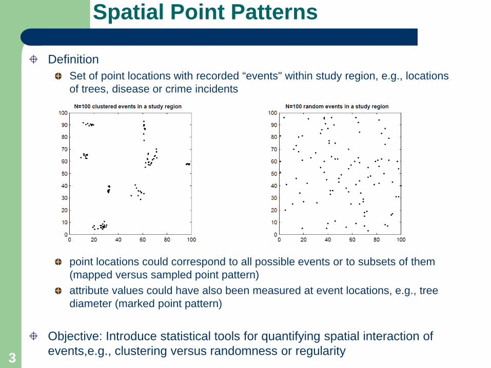
DefinitionSet of point locations with recorded “events" within study region, e.g., locations of trees, disease or crime incidents

point locations could correspond to all possible events or to subsets of them (mapped versus sampled point pattern)attribute values could have also been measured at event locations, e.g., tree diameter (marked point pattern)

Objective: Introduce statistical tools for quantifying spatial interaction of events,e.g., clustering versus randomness or regularity

4

1D Kernel Density Estimation Flowchart

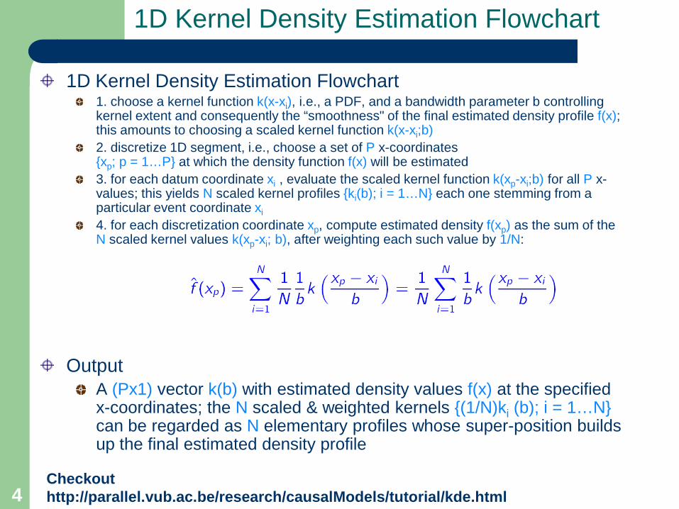
1D Kernel Density Estimation Flowchart1. choose a kernel function k(x-xi), i.e., a PDF, and a bandwidth parameter b controlling kernel extent and consequently the “smoothness" of the final estimated density profile f(x); this amounts to choosing a scaled kernel function k(x-xi;b)2. discretize 1D segment, i.e., choose a set of P x-coordinates {xp; p = 1…P} at which the density function f(x) will be estimated3. for each datum coordinate xi , evaluate the scaled kernel function k(xp-xi;b) for all P x-values; this yields N scaled kernel profiles {ki(b); i = 1…N} each one stemming from a particular event coordinate xi4. for each discretization coordinate xp, compute estimated density f(xp) as the sum of the N scaled kernel values k(xp-xi; b), after weighting each such value by 1/N:

OutputA (Px1) vector k(b) with estimated density values f(x) at the specified x-coordinates; the N scaled & weighted kernels {(1/N)ki (b); i = 1…N} can be regarded as N elementary profiles whose super-position builds up the final estimated density profile

Checkouthttp://parallel.vub.ac.be/research/causalModels/tutorial/kde.html

5

Constructing A Separable 2D Kernel

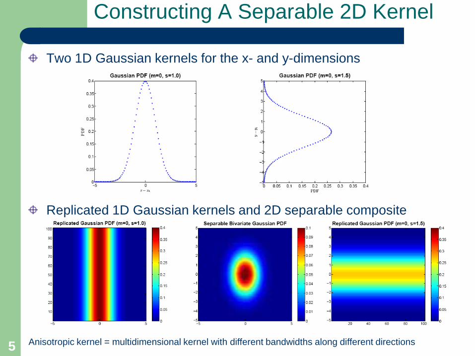
Two 1D Gaussian kernels for the x- and y-dimensions

Replicated 1D Gaussian kernels and 2D separable composite

Anisotropic kernel = multidimensional kernel with different bandwidths along different directions

6

2D Kernel Intensity Estimation

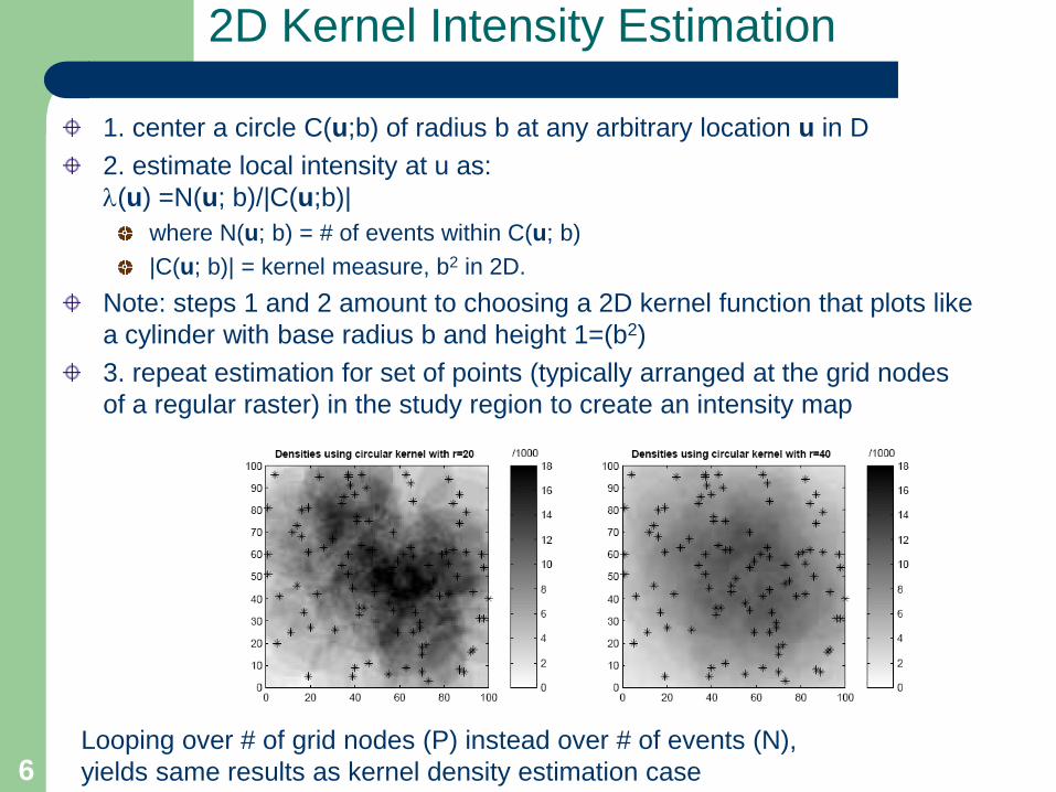
1. center a circle C(u;b) of radius b at any arbitrary location u in D2. estimate local intensity at u as: λ(u) =N(u; b)/|C(u;b)|

where N(u; b) = # of events within C(u; b)|C(u; b)| = kernel measure, b2 in 2D.

Note: steps 1 and 2 amount to choosing a 2D kernel function that plots like a cylinder with base radius b and height 1=(b2)3. repeat estimation for set of points (typically arranged at the grid nodes of a regular raster) in the study region to create an intensity map

Looping over # of grid nodes (P) instead over # of events (N),yields same results as kernel density estimation case

7

Recap (Lecture 3)

Event intensity of spatial point patternsλ(u): mean # of events over a unit area centered at uestimated overall intensity λ = N/|D|local intensity via quadrat counts or kernel density estimation

Kernel intensity estimationconversion of point data (events) to raster format (intensity surface)statistical multidimensional (multivariate) density estimation methods are used to estimate local intensity f(u). Note: Density surface integrates to 1, so multiply every such estimate f(u) by N to convert it to an intensity value f(u)resulting intensity surface depends on: (i) kernel type, and (ii) bandwidth; the latter is more influentialalternative approaches for non-parametric multivariate density estimation include: k-nearest neighbor and mixture of Gaussian densities methodsintensity surface can be linked (via regression models) to explanatory variables, e.g., disease occurrence intensity as function of air quality variables

8

Outline-Lecture 5

Concepts & NotationDistance & Distance MatricesDistances Involved in Spatial Point PatternsStatistical Tests –

Sampling Distributions Bootstrap exampleQuadrat count example

Quantifying Spatial Interaction: Nearest Neighbor Distance Metrics G Function

Proportion of minimum event-to-nearest-event distances no greater than given distance cutoff d

F FunctionProportion of minimum point-to-nearest-event distances no greater than given distance cutoff d

Measures based on the distribution of event intensities The K function Quadrat counts and KS-test?

Quantifying Spatial Interaction: K FunctionPoints To Remember

9

Some Notation

Point eventsSet of N locations of events occurring in a study area:

Variable of interesty(s) = number of events (a count) within arbitrary domain or support s with measure (length, area, volume) |s|; support s is centered at an arbitrary location u and can also be denoted as s(u); in statistics, y(s) is treated as a realization of a random variable (RV) Y(s)

ObjectiveQuantify interaction, e.g., covariation, between outcomes of any two RVs Y(s) and Y(s’). To do so, all RVs must lie in the same “environment"; in other words, the long-term average (expectation) of RV Y(s) should be similar to that of Y(s’)

10

Intensity of Events

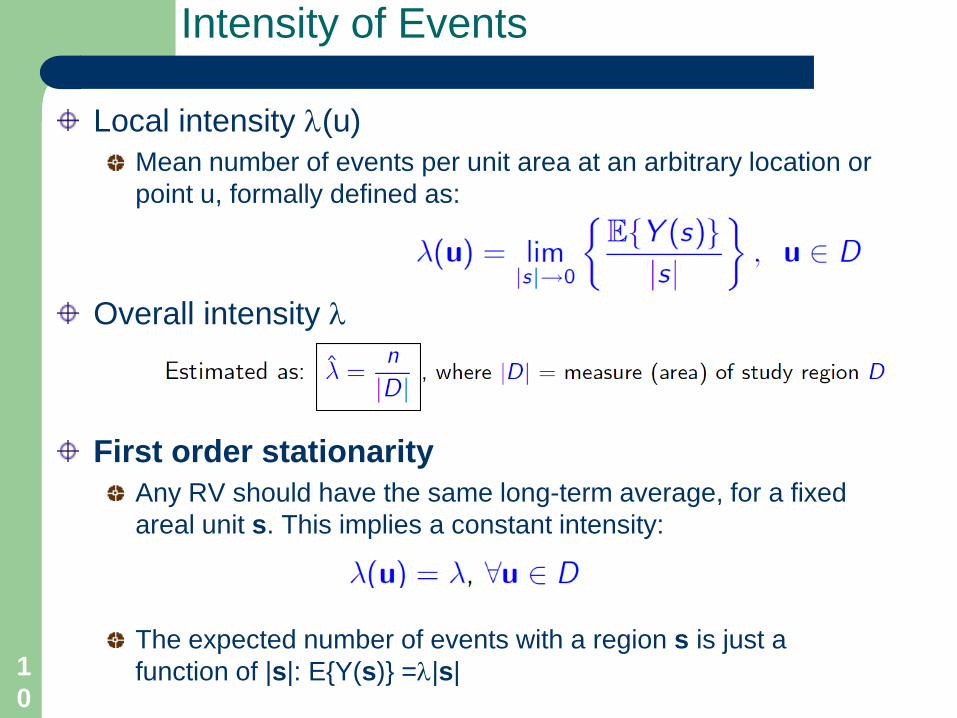
Local intensity λ(u)Mean number of events per unit area at an arbitrary location or point u, formally defined as:

Overall intensity λ

First order stationarityAny RV should have the same long-term average, for a fixed areal unit s. This implies a constant intensity:

The expected number of events with a region s is just a function of |s|: E{Y(s)} =λ|s|

11

Interaction Between Count RVs

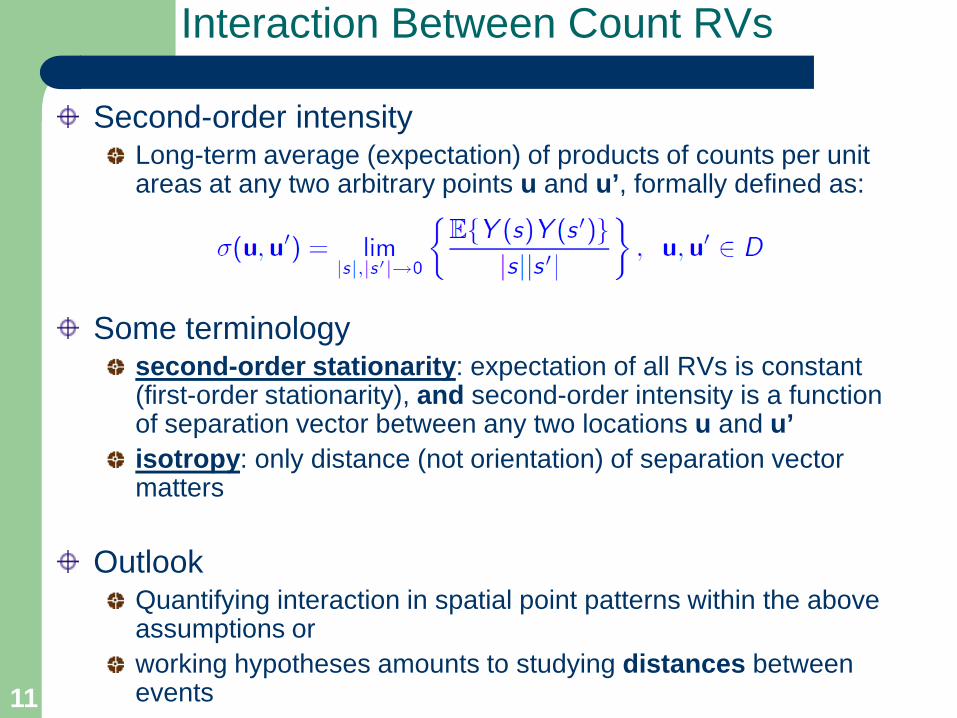
Second-order intensityLong-term average (expectation) of products of counts per unit areas at any two arbitrary points u and u’, formally defined as:

Some terminologysecond-order stationarity: expectation of all RVs is constant (first-order stationarity), and second-order intensity is a function of separation vector between any two locations u and u’isotropy: only distance (not orientation) of separation vector matters

OutlookQuantifying interaction in spatial point patterns within the above assumptions orworking hypotheses amounts to studying distances between events

12

Distance

A measure of proximity (typically along a crow's flight path) between any two locations or spatial entitiesEuclidean distance

Consider two points in a 2D (geographical or other) space with coordinates ui = (xi;yi) and uj = (xj;yj). The Euclidean distance dij between points ui and uj is computed via Pythagoras's theorem as:

13

Distance Metric

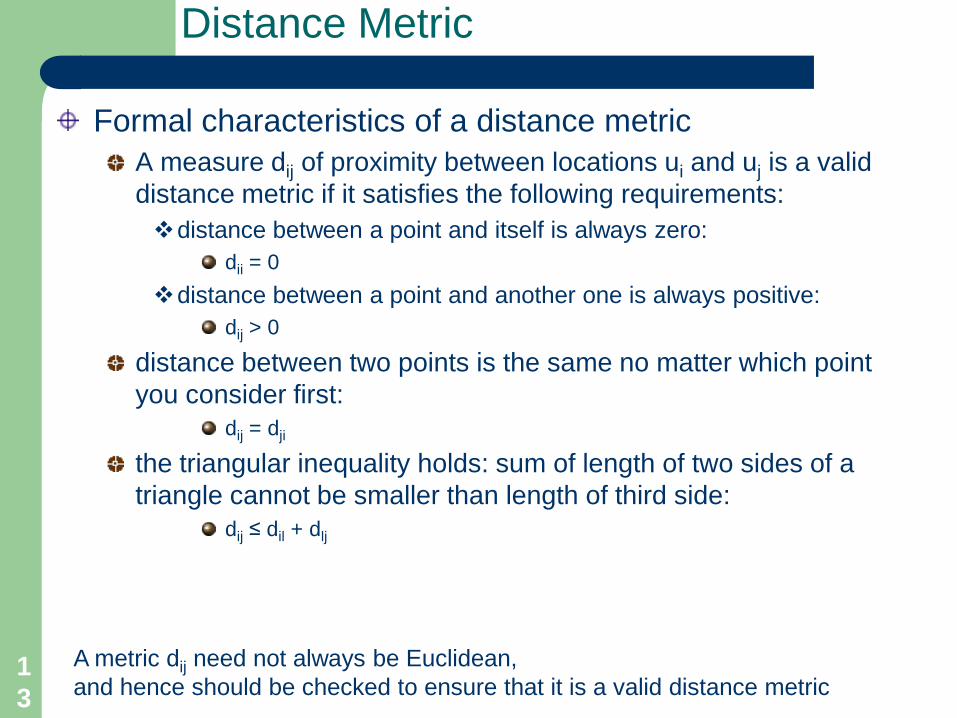
Formal characteristics of a distance metricA measure dij of proximity between locations ui and uj is a valid distance metric if it satisfies the following requirements:distance between a point and itself is always zero:

dii = 0distance between a point and another one is always positive:

dij > 0

distance between two points is the same no matter which point you consider first:

dij = dji

the triangular inequality holds: sum of length of two sides of a triangle cannot be smaller than length of third side:

dij ≤ dil + dlj

A metric dij need not always be Euclidean,and hence should be checked to ensure that it is a valid distance metric

14

Non-Euclidean Distances

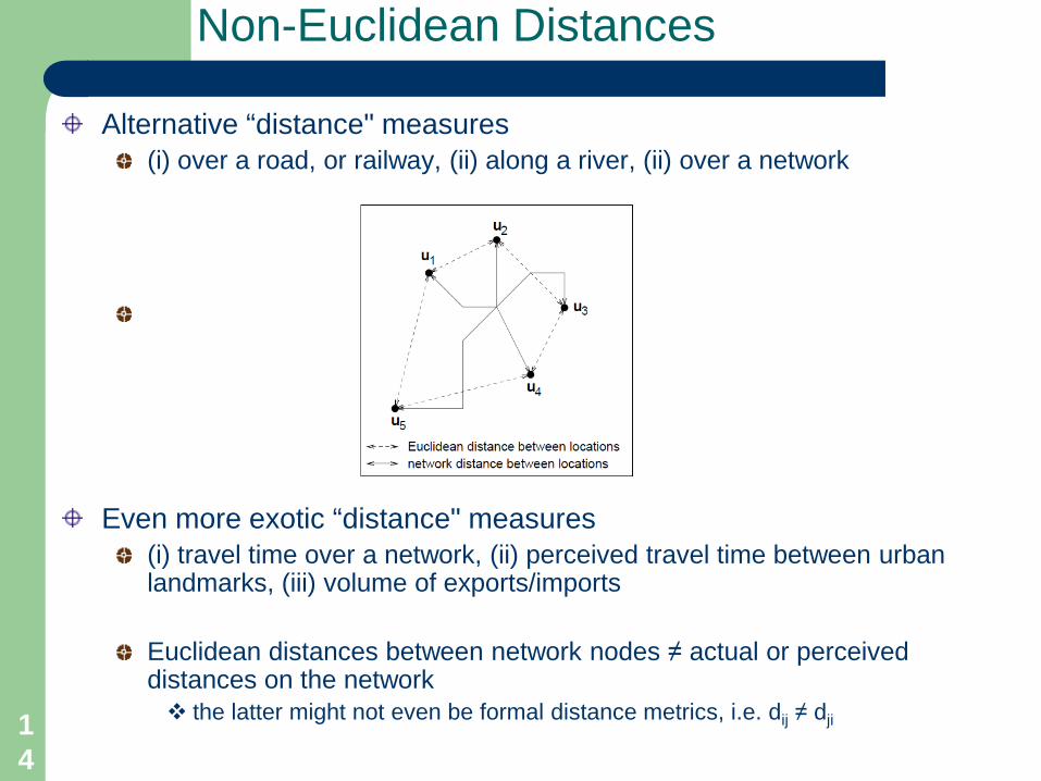
Alternative “distance" measures(i) over a road, or railway, (ii) along a river, (ii) over a network

Even more exotic “distance" measures(i) travel time over a network, (ii) perceived travel time between urban landmarks, (iii) volume of exports/imports

Euclidean distances between network nodes ≠ actual or perceived distances on the network the latter might not even be formal distance metrics, i.e. dij ≠ dji

15

Minkowski's Generalized Distance

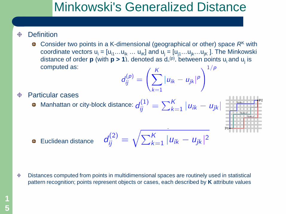
DefinitionConsider two points in a K-dimensional (geographical or other) space RK with coordinate vectors ui = [ui1…uik … uiK] and uj = [uj1…ujk…ujK ]. The Minkowski distance of order p (with p > 1), denoted as dij

(p), between points ui and uj is computed as:

Particular casesManhattan or city-block distance:

Euclidean distance

Distances computed from points in multidimensional spaces are routinely used in statistical pattern recognition; points represent objects or cases, each described by K attribute values

16

Euclidean Distance Matrix: Single Set of Points

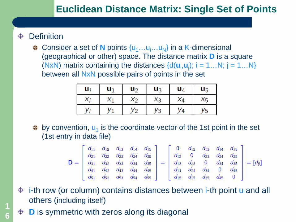
DefinitionConsider a set of N points {u1…ui…uN} in a K-dimensional (geographical or other) space. The distance matrix D is a square (NxN) matrix containing the distances {d(ui,uj); i = 1…N; j = 1…N} between all NxN possible pairs of points in the set

by convention, u1 is the coordinate vector of the 1st point in the set (1st entry in data file)

i-th row (or column) contains distances between i-th point ui and all others (including itself)D is symmetric with zeros along its diagonal

17

Euclidean Distance Matrix: Two Sets of Points

Consider 2 sets of points {u1…ui…uN} and {t1…ti…tM} in a K-dimensional (geographical or other) space. The distance matrix D is a (NxM) matrix containing the Euclidean distances {d(ui,tj); i = 1…N; j = 1…M} between all N x M possible pairs formed by these two sets of points

by convention, u1 is the coordinate vector of the 1st datum in the data set #1, and similarly for t1

i-th row contains distances between i-th point ui in set #1 and all points in set #2j-th column contains distances between j-th point tj in set #2 and all points in set #1

D is not symmetric, i.e., d12 ≠ d21: pair {u1,t2} is not the same as pair {u2,t1}

18

Distances Between Events in A Point Pattern

Event-to-event distanceDistance dij between event at location ui and another event at location uj

Point-to-event distanceDistance dpj between a randomly chosen point at location tp and an event at location uj :

Event-to-nearest-event distanceDistance dmin(ui) between an event at location ui and its nearest neighbor event:

Point-to-nearest-event distanceDistance dmin(tp) between a randomly chosen point at location tp and its nearest neighbor event:

19

Event-to-Nearest-Event Distances

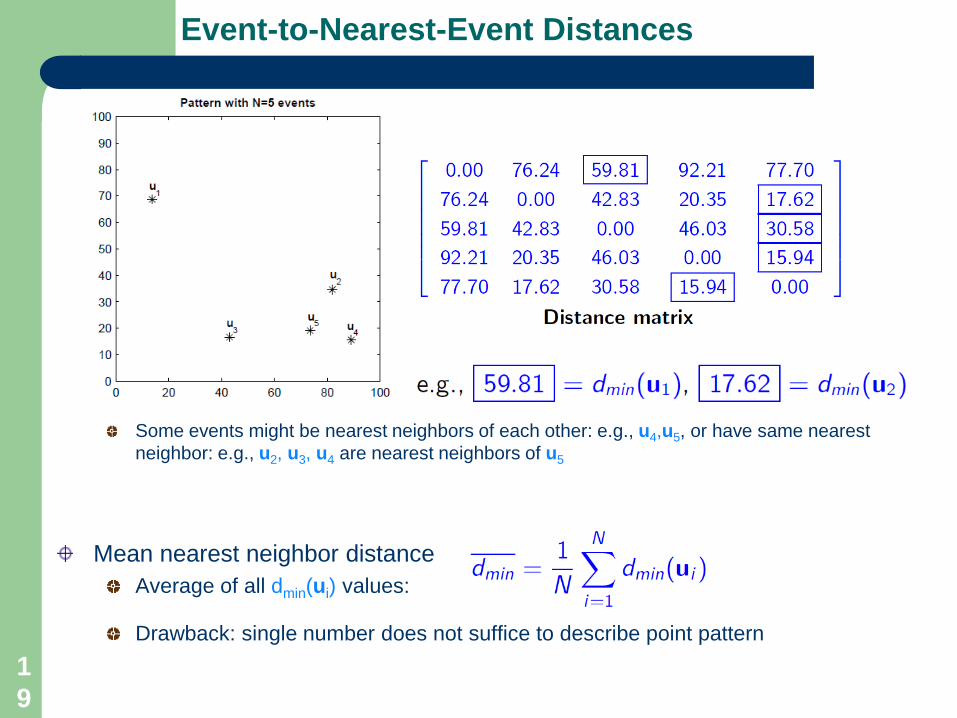
Some events might be nearest neighbors of each other: e.g., u4,u5, or have same nearest neighbor: e.g., u2, u3, u4 are nearest neighbors of u5

Mean nearest neighbor distanceAverage of all dmin(ui) values:

Drawback: single number does not suffice to describe point pattern

20

The G Function

DefinitionProportion of event-to-nearest-event distances dmin(ui) no greater than given distance cutoff d, estimated as:

Cumulative distribution function (CDF) of all N event-to-nearest-event distances

Example

21

Event-to-Nearest-Event (E2NE) Distance Histograms

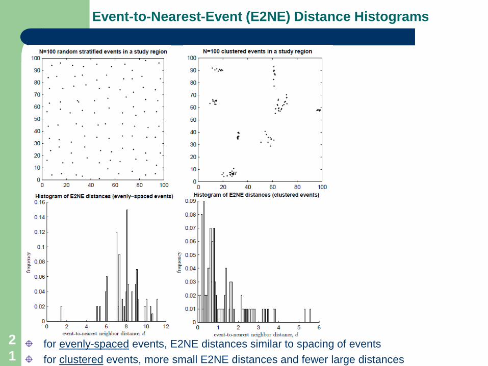
for evenly-spaced events, E2NE distances similar to spacing of eventsfor clustered events, more small E2NE distances and fewer large distances

Point Pattern Analysis Metrics

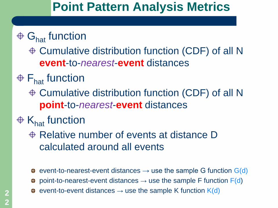
Ghat functionCumulative distribution function (CDF) of all N event-to-nearest-event distances

Fhat functionCumulative distribution function (CDF) of all N point-to-nearest-event distances

Khat functionRelative number of events at distance D calculated around all events

event-to-nearest-event distances → use the sample G function G(d)point-to-nearest-event distances → use the sample F function F(d)event-to-event distances → use the sample K function K(d)2

2

23

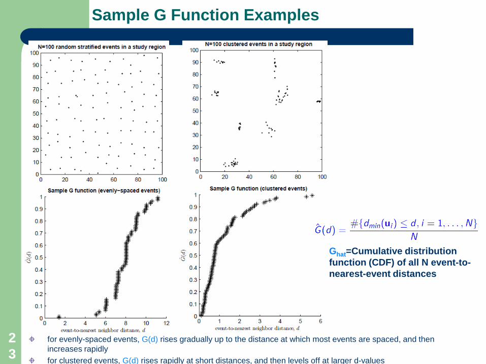
Sample G Function Examples

for evenly-spaced events, G(d) rises gradually up to the distance at which most events are spaced, and then increases rapidlyfor clustered events, G(d) rises rapidly at short distances, and then levels off at larger d-values

Ghat=Cumulative distribution function (CDF) of all N event-to-nearest-event distances

24

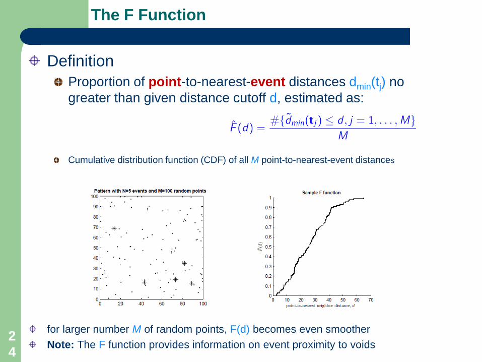
The F Function

DefinitionProportion of point-to-nearest-event distances dmin(tj) no greater than given distance cutoff d, estimated as:

Cumulative distribution function (CDF) of all M point-to-nearest-event distances

for larger number M of random points, F(d) becomes even smootherNote: The F function provides information on event proximity to voids

25

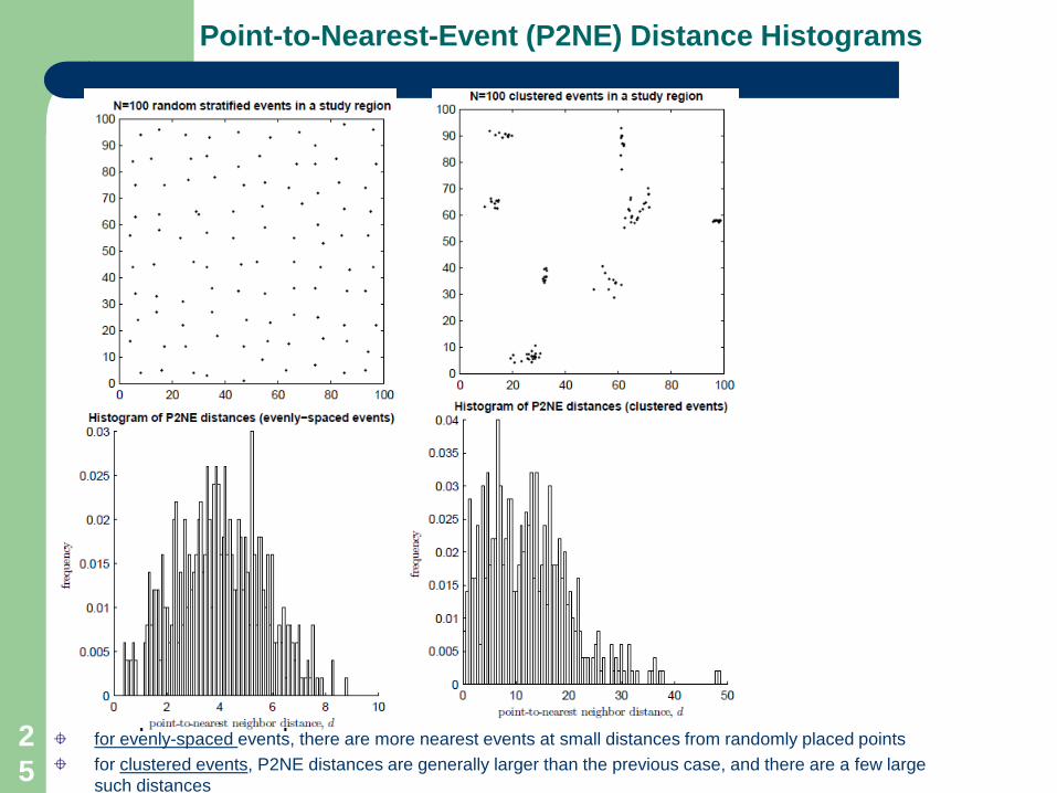
Point-to-Nearest-Event (P2NE) Distance Histograms

for evenly-spaced events, there are more nearest events at small distances from randomly placed pointsfor clustered events, P2NE distances are generally larger than the previous case, and there are a few large such distances

26

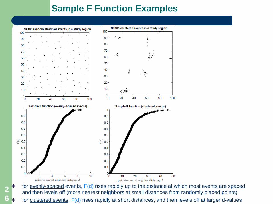
Sample F Function Examples

for evenly-spaced events, F(d) rises rapidly up to the distance at which most events are spaced, and then levels off (more nearest neighbors at small distances from randomly placed points)for clustered events, F(d) rises rapidly at short distances, and then levels off at larger d-values

27

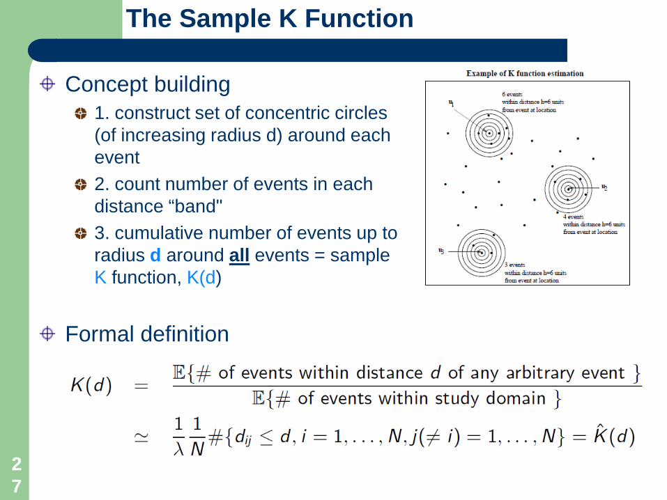
The Sample K Function

Concept building1. construct set of concentric circles (of increasing radius d) around each event2. count number of events in each distance “band"3. cumulative number of events up to radius d around all events = sample K function, K(d)

Formal definition

28

Interpreting The Sample K Function

Re-expressing

In other words: Function K(d) is the sample cumulative distribution function (CDF) of all N2-N event-to-event distances, scaled by |D|

Note: Ignore bin at d = 0 (center plot) and point at d = 0 (right plot

29

Event-to-Event Distance Histograms

for evenly-spaced events, there are more medium-sized E2E distances than small or large such distancesfor clustered events, the distribution of E2E distances is multi-modal

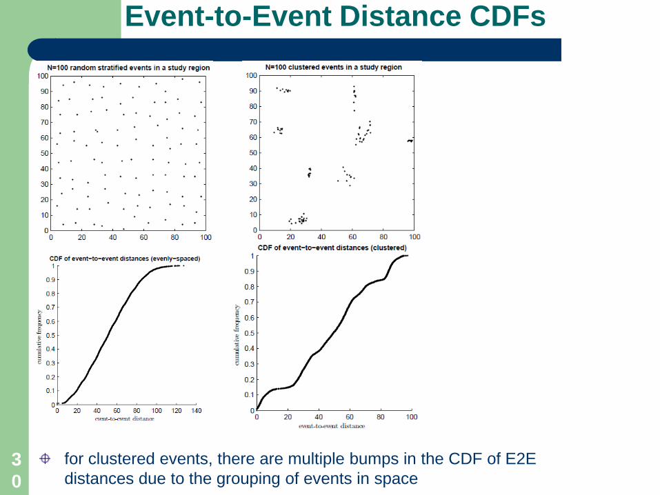
Event-to-Event Distance CDFs

for clustered events, there are multiple bumps in the CDF of E2E distances due to the grouping of events in space

30

31

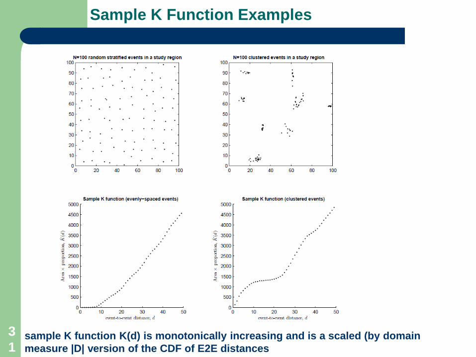
Sample K Function Examples

sample K function K(d) is monotonically increasing and is a scaled (by domainmeasure |D| version of the CDF of E2E distances

32

Recap

Quantifying interaction in spatial point patternsevent-to-nearest-event distances → use the sample G function G(d)point-to-nearest-event distances → use the sample F function F(d)event-to-event distances → use the sample K function K(d)K function looks at information beyond nearest neighbors

Caveatsclustering is always a function of the overall intensity of a point patternclustering might occur due to local intensity variations or due to interaction;it is very difficult to disentangle each contribution

Watch out forboundaries and edge effectsdistance distortions due to map projectionssampled versus mapped point patternsInteractions of 1st versus second order stationarity