interactive multiresolution mesh editing
TRANSCRIPT
Interactive Multiresolution Mesh Editing
Denis Zorin�
Caltech
Peter Schr�odery
Caltech
Wim Sweldensz
Bell Laboratories
Abstract
We describe a multiresolution representation for meshes based on subdivision. Subdivision is anatural extension of the existing patch-based surface representations. At the same time subdivisionalgorithms can be viewed as operating directly on polygonal meshes, which makes them a useful toolfor mesh manipulation. Combination of subdivision and smoothing algorithms of Taubin [26] allowsus to construct a set of algorithms for interactive multiresolution editing of complex meshes of arbi-trary topology. Simplicity of the essential algorithms for re�nement and coarsi�cation allows to makethem local and adaptive, considerably improving their e�ciency. We have built a scalable interactivemultiresolution editing system based on such algorithms.
1 Introduction
Applications such as special e�ects and animation require the creation and manipulation of complex ge-ometric models of arbitrary topology. Like real world geometry, these models often carry detail at manyscales (cf. Fig. 1). The model might be constructed from scratch (ab initio design) in an interactive mod-eling environment or be scanned-in either by hand or with automatic digitizing methods. The latter is acommon source of data particularly in the entertainment industry. When using laser range scanners, forexample, individual models are often composed of high resolution meshes with hundreds of thousands tomillions of polygons.Manipulating such �ne meshes can be di�cult, especially when they are to be edited or animated.
Interactivity, which is crucial in these cases, is challenging to achieve. Even without accounting for anycomputation on the mesh itself, available rendering resources alone, may not be able to cope with the sheersize of the data. Possible approaches include mesh optimization [16, 14] to reduce the size of the meshes.Aside from considerations of economy, the choice of representation is also guided by the need for mul-
tiresolution editing semantics. The representation of the mesh needs to provide control at a large scale,so that one can change the mesh in a broad, smooth manner, for example. Additionally designers willtypically also want control over the minute features of the model (cf. Fig. 1). Smoother approximationscan be built through the use of patches [15], though at the cost of loosing the high frequency details. Suchdetail can be reintroduced by combining patches with displacement maps [18]. However, this is di�cult tomanage in the arbitrary topology setting and across a continuous range of scales and hardware resources.
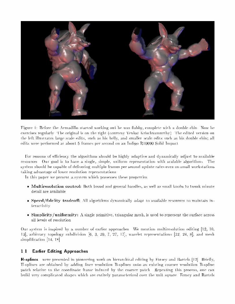
Figure 1: Before the Armadillo started working out he was abby, complete with a double chin. Now heexercises regularly. The original is on the right (courtesy Venkat Krischnamurthy). The edited version onthe left illustrates large scale edits, such as his belly, and smaller scale edits such as his double chin; alledits were performed at about 5 frames per second on an Indigo R10000 Solid Impact.
For reasons of e�ciency the algorithms should be highly adaptive and dynamically adjust to availableresources. Our goal is to have a single, simple, uniform representation with scalable algorithms. Thesystem should be capable of delivering multiple frames per second update rates even on small workstationstaking advantage of lower resolution representations.In this paper we present a system which possesses these properties
� Multiresolution control: Both broad and general handles, as well as small knobs to tweak minutedetail are available.
� Speed/�delity tradeo�: All algorithms dynamically adapt to available resources to maintain in-teractivity.
� Simplicity/uniformity: A single primitive, triangular mesh, is used to represent the surface acrossall levels of resolution.
Our system is inspired by a number of earlier approaches. We mention multiresolution editing [12, 10,13], arbitrary topology subdivision [6, 3, 20, 7, 27, 17], wavelet representations [22, 24, 8], and meshsimpli�cation [14, 18].
1.1 Earlier Editing Approaches
H-splines were presented in pioneering work on hierarchical editing by Forsey and Bartels [12]. Brie y,H-splines are obtained by adding �ner resolution B-splines onto an existing coarser resolution B-splinepatch relative to the coordinate frame induced by the coarser patch. Repeating this process, one canbuild very complicated shapes which are entirely parameterized over the unit square. Forsey and Bartels
observed that the hierarchy induced coordinate frame for the o�sets is essential to achieve correct editingsemantics.H-splines provide a uniform framework for representing both the coarse and �ne level details. Note
however, that as more detail is added to such a model the internal control mesh data structures more andmore resemble a �ne polyhedral mesh.
While their original implementation allowed only for regular topologies their approach could be extendedto the general setting by using surface splines or one of the spline derived general topology subdivisionschemes [19]. However, these schemes have not yet been made to work adaptively.Forsey and Bartels' original work focused on the ab initio design setting. There the user's help is
enlisted in de�ning what is meant by di�erent levels of resolution. The user decides where to add detailand manipulates the corresponding controls. This way the levels of the hierarchy are hand built by ahuman user and the representation of the �nal object is a function of its editing history.
To edit an a priori given model it is crucial to have a general procedure to de�ne coarser levels andcompute details between levels. We refer to this as the analysis algorithm. An H-spline analysis algorithmbased on weighted least squares was introduced [11], but is too expensive to run interactively. Note thateven in an ab initio design setting online analysis is needed, since after a long sequence of editing steps theH-spline is likely to be overly re�ned and needs to be consolidated.
Wavelets provide a framework in which to rigorously de�ne multiresolution approximations and fastanalysis algorithms. Finkelstein and Salesin [10], for example, used B-spline wavelets to describe mul-tiresolution editing of curves. As in H-splines, parameterization of details with respect to a coordinateframe induced by the coarser level approximation is required to get correct editing semantics. Gortler andCohen [13], pointed out that wavelet representations of detail tend to behave in undesirable ways duringediting and returned to a pure B-spline representation as used in H-splines.Carrying these constructions over into the arbitrary topology surface framework is not straightforward.
In pioneering work by Lounsbery et al. [22] the connection between wavelets and subdivision was usedto de�ne the di�erent levels of resolution. The original constructions were limited to piecewise linearsubdivision, but smoother constructions are possible [24, 27].The introduction of analysis algorithms and the connection with subdivision were the main contributions
of wavelets to multiresolution editing. Subdivision, however, relies on the �nest level mesh having subdivi-sion connectivity. This requires a remeshing step before external high resolution geometry can be importedinto the editor. Eck et al. [9] have described a possible approach to remeshing arbitrary �nest level inputmeshes fully automatically. A method that relies on a user's expertise was developed by Krishnamurthyand Levoy [18]. They wanted to build coarse B-spline patch approximations, augmented with displacementmaps, to preprocess laser range scanner data for later animation. Since models built from B-spline patcheswill exhibit problems along patch boundaries, especially when animated, user speci�cation of the patchboundaries is important in their setting.Before we proceed to a more detailed discussion of editing we �rst discuss di�erent surface representations
to motivate our choice of synthesis (re�nement) algorithm.
1.2 Surface Representations
There are many possible choices for surface representations. Among the most popular are polynomialpatches and polygons.
Patches are a powerful primitive for the construction of coarse grain, smooth models using a small numberof control parameters. Combined with hardware support relatively fast implementations are possible.However, when building complex models with many patches the preservation of smoothness across patchboundaries can be quite cumbersome and expensive. These di�culties are compounded in the arbitrary
topology setting when polynomial parameterizations cease to exist everywhere. Surface splines [4, 21, 23]provide one way to address the arbitrary topology challenge.As more �ne level detail is needed the proliferation of control points and patches can quickly overwhelm
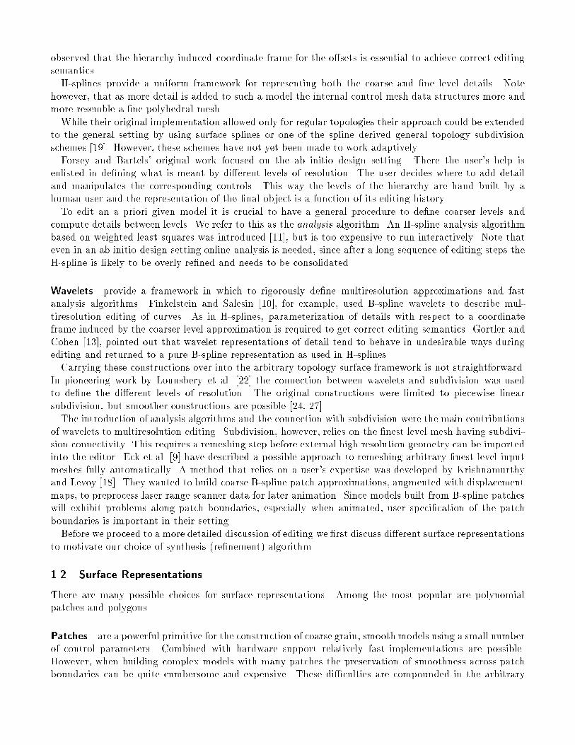
both the user and the most powerful hardware. With detail at �ner levels, patches become less suited andpolygonal meshes are more appropriate (cf. Fig. 2).
Figure 2: What used to be a patch is best treated as a mesh when adding �ne detail.
Polygonal Meshes can represent arbitrary topology and resolve �ne detail as found in laser scannedmodels, for example. Given that most hardware rendering ultimately resolves to triangle scan-conversioneven for patches, polygonal meshes are a very basic primitive. Because of sheer size, polygonal meshesare di�cult to manipulate interactively. Mesh simpli�cation algorithms [14] provide one possible answer.However, we need a mesh simpli�cation approach, which is hierarchical and gives us shape handles forsmooth changes over larger regions while maintaining high frequency details.
Patches Fine Polyhedra
Subdivision
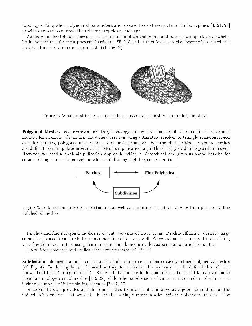
Figure 3: Subdivision provides a continuous as well as uniform description ranging from patches to �nepolyhedral meshes.
Patches and �ne polygonal meshes represent two ends of a spectrum. Patches e�ciently describe largesmooth sections of a surface but cannot model �ne detail very well. Polygonal meshes are good at describingvery �ne detail accurately using dense meshes, but do not provide coarser manipulation semantics.Subdivision connects and uni�es these two extremes (cf. Fig. 3).
Subdivision de�nes a smooth surface as the limit of a sequence of successively re�ned polyhedral meshes(cf. Fig. 4). In the regular patch based setting, for example, this sequence can be de�ned through wellknown knot insertion algorithms [5]. Some subdivision methods generalize spline based knot insertion toirregular topology control meshes [3, 6, 20] while other subdivision schemes are independent of splines andinclude a number of interpolating schemes [7, 27, 17].Since subdivision provides a path from patches to meshes, it can serve as a good foundation for the
uni�ed infrastructure that we seek. Internally, a single representation exists: polyhedral meshes. The
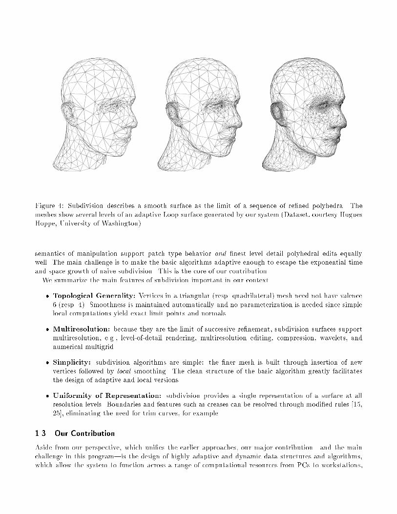
Figure 4: Subdivision describes a smooth surface as the limit of a sequence of re�ned polyhedra. Themeshes show several levels of an adaptive Loop surface generated by our system (Dataset, courtesy HuguesHoppe, University of Washington)
semantics of manipulation support patch type behavior and �nest level detail polyhedral edits equallywell. The main challenge is to make the basic algorithms adaptive enough to escape the exponential timeand space growth of naive subdivision. This is the core of our contribution.
We summarize the main features of subdivision important in our context
� Topological Generality: Vertices in a triangular (resp. quadrilateral) mesh need not have valence6 (resp. 4). Smoothness is maintained automatically and no parameterization is needed since simplelocal computations yield exact limit points and normals.
� Multiresolution: because they are the limit of successive re�nement, subdivision surfaces supportmultiresolution, e.g., level-of-detail rendering, multiresolution editing, compression, wavelets, andnumerical multigrid.
� Simplicity: subdivision algorithms are simple: the �ner mesh is built through insertion of newvertices followed by local smoothing. The clean structure of the basic algorithm greatly facilitatesthe design of adaptive and local versions.
� Uniformity of Representation: subdivision provides a single representation of a surface at allresolution levels. Boundaries and features such as creases can be resolved through modi�ed rules [15,25], eliminating the need for trim curves, for example.
1.3 Our Contribution
Aside from our perspective, which uni�es the earlier approaches, our major contribution|and the mainchallenge in this program|is the design of highly adaptive and dynamic data structures and algorithms,which allow the system to function across a range of computational resources from PCs to workstations,
delivering as much interactive �delity as possible with a given polygon rendering performance. Our algo-rithms work for the class of 1-ring subdivision schemes (de�nition see below) and we demonstrate theirperformance for the concrete case of Loop's subdivision scheme.
We chose subdivision as the basis for our mesh geometry editor, since it enables multiresolution, worksin the arbitrary topology setting, spans the scales from large patches to �ne polygonal geometry, and canbe made fast enough to provide interactive performance.
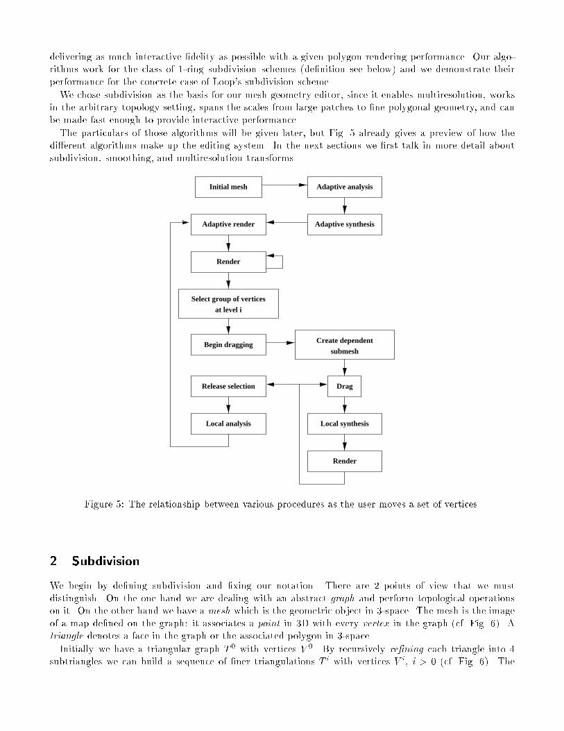
The particulars of those algorithms will be given later, but Fig. 5 already gives a preview of how thedi�erent algorithms make up the editing system. In the next sections we �rst talk in more detail aboutsubdivision, smoothing, and multiresolution transforms.
submesh
Select group of vertices
at level i
Initial mesh
Create dependentBegin dragging
Adaptive synthesis
Adaptive analysis
Render
Adaptive render
Release selection
Local analysis
Drag
Local synthesis
Render
Figure 5: The relationship between various procedures as the user moves a set of vertices.
2 Subdivision
We begin by de�ning subdivision and �xing our notation. There are 2 points of view that we mustdistinguish. On the one hand we are dealing with an abstract graph and perform topological operationson it. On the other hand we have a mesh which is the geometric object in 3-space. The mesh is the imageof a map de�ned on the graph: it associates a point in 3D with every vertex in the graph (cf. Fig. 6). Atriangle denotes a face in the graph or the associated polygon in 3-space.
Initially we have a triangular graph T 0 with vertices V 0. By recursively re�ning each triangle into 4subtriangles we can build a sequence of �ner triangulations T i with vertices V i, i > 0 (cf. Fig. 6). The
1 2
3re
fine
men
t subdivision
3
1 2
s (6)
i+1
i+1
i+1
i+1i+1
i+1
s (3)
s (5)
s (2)
s (4)s (1)4
i+1T
s (2)is (1)
Vi
V i+1
s (3)i
i
6 5
T i
Graph with vertices Mesh with points
Maps to
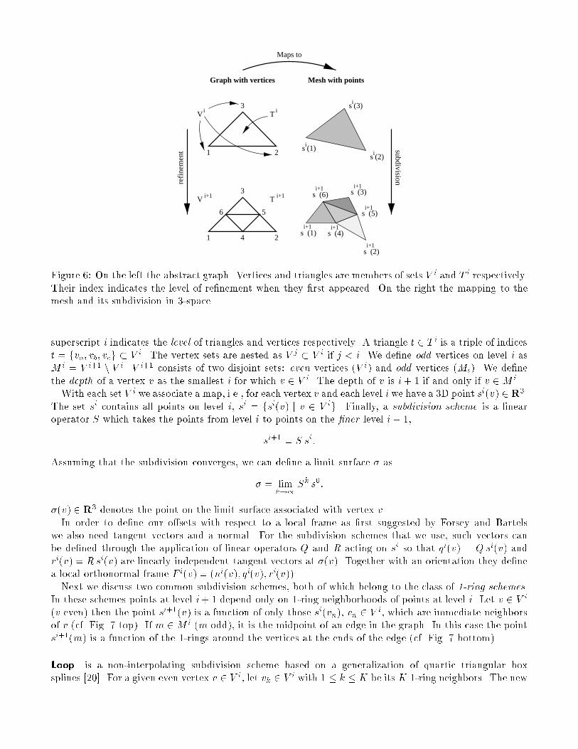
Figure 6: On the left the abstract graph. Vertices and triangles are members of sets V i and T i respectively.Their index indicates the level of re�nement when they �rst appeared. On the right the mapping to themesh and its subdivision in 3-space.
superscript i indicates the level of triangles and vertices respectively. A triangle t 2 T i is a triple of indicest = fva; vb; vcg � V i. The vertex sets are nested as V j � V i if j < i. We de�ne odd vertices on level i asM i = V i+1 n V i. V i+1 consists of two disjoint sets: even vertices (V i) and odd vertices (Mi). We de�nethe depth of a vertex v as the smallest i for which v 2 V i. The depth of v is i+ 1 if and only if v 2M i.With each set V i we associate a map, i.e., for each vertex v and each level i we have a 3D point si(v) 2 R3.
The set si contains all points on level i, si = fsi(v) j v 2 V ig. Finally, a subdivision scheme is a linearoperator S which takes the points from level i to points on the �ner level i+ 1,
si+1 = S si:
Assuming that the subdivision converges, we can de�ne a limit surface � as
� = limk!1
Sk s0:
�(v) 2 R3 denotes the point on the limit surface associated with vertex v.In order to de�ne our o�sets with respect to a local frame as �rst suggested by Forsey and Bartels
we also need tangent vectors and a normal. For the subdivision schemes that we use, such vectors canbe de�ned through the application of linear operators Q and R acting on si so that qi(v) = Qsi(v) andri(v) = Rsi(v) are linearly independent tangent vectors at �(v). Together with an orientation they de�nea local orthonormal frame F i(v) = (ni(v); qi(v); ri(v)).Next we discuss two common subdivision schemes, both of which belong to the class of 1-ring schemes.
In these schemes points at level i+ 1 depend only on 1-ring neighborhoods of points at level i. Let v 2 V i
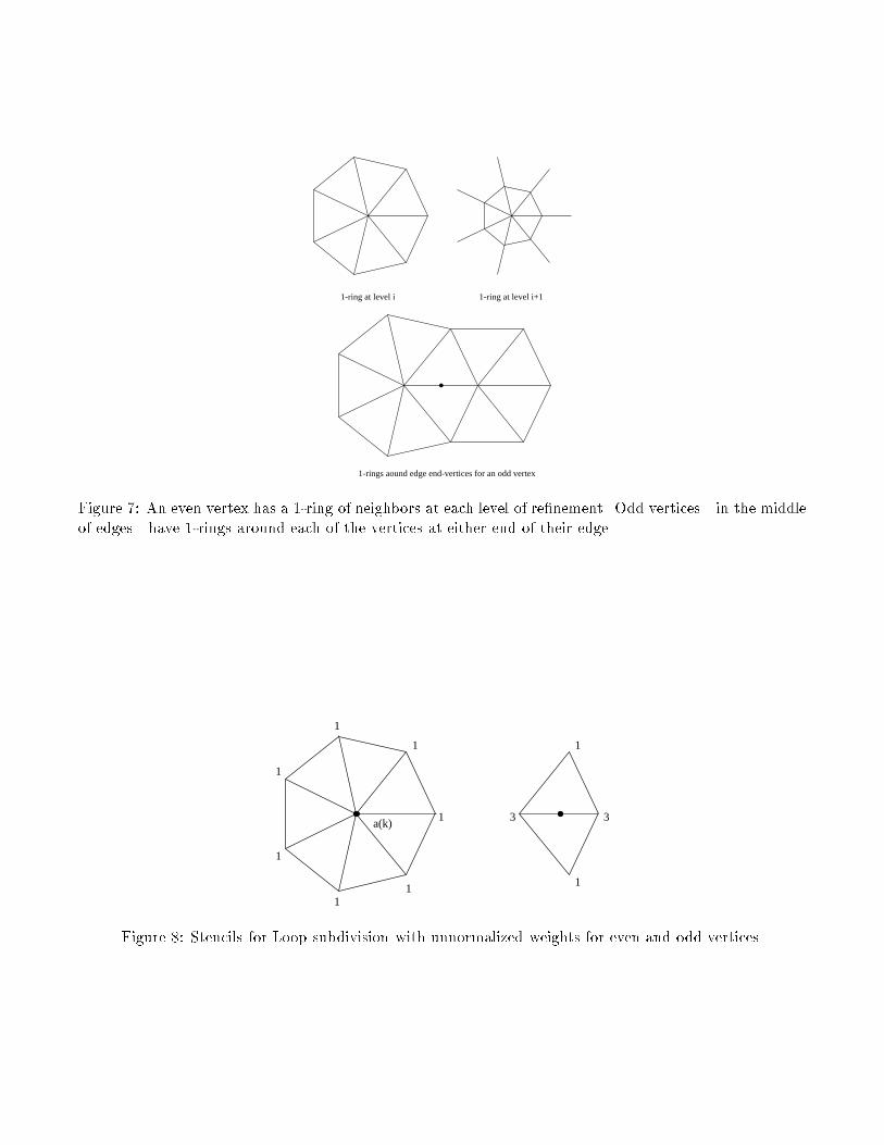
(v even) then the point si+1(v) is a function of only those si(vn), vn 2 V i, which are immediate neighborsof v (cf. Fig. 7 top). If m 2M i (m odd), it is the midpoint of an edge in the graph. In this case the pointsi+1(m) is a function of the 1-rings around the vertices at the ends of the edge (cf. Fig. 7 bottom).
Loop is a non-interpolating subdivision scheme based on a generalization of quartic triangular boxsplines [20]. For a given even vertex v 2 V i, let vk 2 V i with 1 � k � K be its K 1-ring neighbors. The new
1-ring at level i 1-ring at level i+1
1-rings aound edge end-vertices for an odd vertex
Figure 7: An even vertex has a 1-ring of neighbors at each level of re�nement. Odd vertices|in the middleof edges|have 1-rings around each of the vertices at either end of their edge.
1
1
1
1
1
1
33
1
11
a(k)
Figure 8: Stencils for Loop subdivision with unnormalized weights for even and odd vertices.
point si+1(v) is de�ned as si+1(v) = (a(K) +K)�1(a(K) si(v) +PK
k=1 si(vk)) (cf. Fig. 8), a(K) = K(1�
�(K))=�(K), and �(K) = 5=8� (3 + 2 cos(2�=K))2=64. For odd v the weights shown in Fig. 8 are used.The limit point �(v) is given by �(v) = (!(K) +K)�1(!(K) si(v) +
PKk=1 s
i(vk)), !(K) = (3K)=(8�(K)).Two independent tangent vectors t1(v) and t2(v) are given by tp(v) =
PKk=1 cos(2�(k+ p)=K) si(vk).
Features such as boundaries and cusps can be accommodated through simple modi�cations of the stencilweights [15, 25, 1].
Butter y is an interpolating scheme, �rst proposed by Dyn et al. [7] in the topologically regular settingand recently generalized to arbitrary topologies [27]. Since it is interpolating we have si(v) = �(v) forv 2 V i even. For m 2 M i the de�nition of si+1(m) is based on a full stencil as shown in Fig. 7 on thebottom. The exact expressions depend on the valence K and the reader is referred to the original paperfor the exact values [27].
For our implementation we have chosen the Loop scheme, since more performance optimizations arepossible in it. However, the algorithms we discuss later work for any 1-ring scheme.
3 Multiresolution Transforms
So far we only discussed subdivision, i.e., how to go from coarse to �ne meshes. In this section we describeanalysis which goes from �ne to coarse.
We �rst need smoothing, i.e., a linear operation H to build a smooth coarse mesh at level i� 1 from a�ne mesh at level i:
si�1 = H si:
Several options are available here:
� Least squares: One could de�ne analysis to be optimal in the least squares sense,
minsi�1
ksi � S si�1k2:
The solution may have unwanted undulations and is too expensive to compute interactively [11].
� Fairing: A coarse surface could be obtained as the solution to a global variational problem. Thisis too expensive as well. An alternative is presented by Taubin [26], who uses a local non shrinkingsmoothing approach.
Because of its computational simplicity we decided to use the following version of Taubin smoothing. Asbefore let v 2 V i have K neighbors vk 2 V i. Use the average, si(v) = K�1PK
k=1 si(vk), to de�ne the
generalization of the Laplacian L(v) = si(v)� si(v). On this basis Taubin gives a Gaussian-like smootherwhich does not exhibit shrinkage
H := (I + �L) (I + �L):
With subdivision and smoothing in place, we can describe the transform needed to support multires-olution editing. Recall that for multiresolution editing we want the di�erence between successive levelsexpressed with respect to a frame induced by the coarser level, i.e., the o�sets are relative to the smootherlevel.
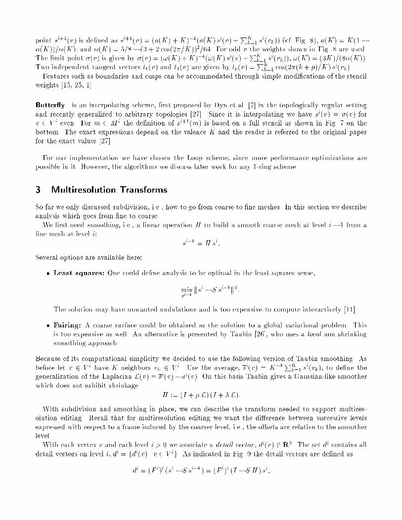
With each vertex v and each level i > 0 we associate a detail vector , di(v) 2 R3. The set di contains alldetail vectors on level i, di = fdi(v) j v 2 V ig. As indicated in Fig. 9 the detail vectors are de�ned as
di = (F i)t (si � S si�1) = (F i)t (I � S H) si;
i.e., the detail vectors at level i record how much the points at level i di�er from the result of subdividingthe points at level i � 1. This di�erence is then computed with respect to the local frame F i to obtaincoordinate independence.Since detail vectors are sampled on the �ne level mesh V i, this transformation yields an overrepresenta-
tion in the same spirit as the Burt-Adelson Laplacian pyramid [2]. The only di�erence is that the smoothing�lters (Taubin) are not the dual of the subdivision �lter (Loop). Theoretically it would be possible to sub-sample the detail vectors and only record a detail per odd vertex of M i�1. This is what happens in thewavelet transform. However, subsampling the details severely restricts the family of smoothing operatorsthat can be used. In an overrepresentation, many di�erent sets of details could yield the same surface.This is not a problem, however, as the analysis algorithm will consistently pick a unique set of details.
Smoothing
i-1is -Ss
Subdivision
i-1s
idis(F )
ti
Figure 9: Wiring diagram of the multiresolution transform.
4 Algorithms and Implementation
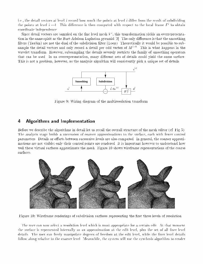
Before we describe the algorithms in detail let us recall the overall structure of the mesh editor (cf. Fig 5).The analysis stage builds a succession of coarser approximations to the surface, each with fewer controlparameters. Details or o�sets between successive levels are also computed. In general, the coarser approxi-mations are not visible; only their control points are rendered. It is important however to understand howwell these virtual surfaces approximate the mesh. Figure 10 shows wireframe representations of the coarsesurfaces.
Figure 10: Wireframe renderings of subdivision surfaces representing the �rst three levels of resolution.
The user can now select a resolution level which is most appropriate for a certain edit. At that momentthe surface is represented internally as an approximation at the edit level, plus the set of all �ner leveldetails. The user can freely manipulate degrees of freedom at the edit level, while the �ner level detailsfollow along relative to the coarser level. Meanwhile, the system will use the synthesis algorithm to render
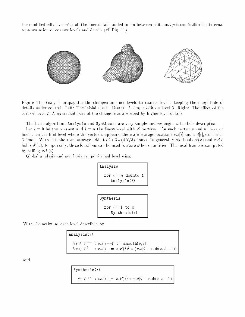
the modi�ed edit level with all the �ner details added in. In between edits analysis consisti�es the internalrepresentation of coarser levels and details (cf. Fig. 11)
Figure 11: Analysis propagates the changes on �ner levels to coarser levels, keeping the magnitude ofdetails under control. Left: The initial mesh. Center: A simple edit on level 3. Right: The e�ect of theedit on level 2. A signi�cant part of the change was absorbed by higher level details.
The basic algorithms Analysis and Synthesis are very simple and we begin with their description.Let i = 0 be the coarsest and i = n the �nest level with N vertices. For each vertex v and all levels i
�ner then the �rst level where the vertex v appears, there are storage locations v:s[i] and v:d[i], each with3 oats. With this the total storage adds to 2 � 3 � (4N=3) oats. In general, v:s[i] holds si(v) and v:d[i]holds di(v); temporarily, these locations can be used to store other quantities. The local frame is computedby calling v:F (i).Global analysis and synthesis are performed level wise:
Analysis
for i = n downto 1
Analysis(i)
Synthesis
for i = 1 to nSynthesis(i)
With the action at each level described by
Analysis(i)
8v 2 V i�1 : v:s[i� 1] := smooth(v; i)8v 2 V i : v:d[i] := v:F (i)t � (v:s[i]� sub(v; i� 1))
and
Synthesis(i)
8v 2 V i : s:v[i] := v:F (i) � v:d[i] + sub(v; i� 1)
Analysis computes points on the coarser level i� 1 using smoothing (smooth), subdivides si�1 (sub), andcomputes the detail vectors di (cf. Fig. 9). Synthesis reconstructs level i by subdividing level i � 1 andadding the details.
So far we have assumed that all levels are uniformly re�ned, i.e., all neighbors at all levels exist. Sincetime and storage costs grow exponentially with the number of levels, this idealized approach is unsuitablefor an interactive implementation. In the next sections we explain how these basic algorithms can be madememory and time e�cient.
Adaptive and local versions of these generic algorithms (cf. Fig. 5 for an overview of their use) are theykey to these savings. The underlying idea is to use lazy evaluation and pruning based on thresholds. Threethresholds control this pruning: �A for adaptive analysis, �S for adaptive synthesis, and �R for adaptiverendering. To make lazy evaluation fast enough several caches are maintained explicitly and the order ofcomputations is carefully staged to avoid recomputation.
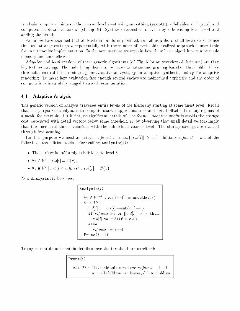
4.1 Adaptive Analysis
The generic version of analysis traverses entire levels of the hierarchy starting at some �nest level. Recallthat the purpose of analysis is to compute coarser approximations and detail o�sets. In many regions ofa mesh, for example, if it is at, no signi�cant details will be found. Adaptive analysis avoids the storagecost associated with detail vectors below some threshold �A by observing that small detail vectors implythat the �ner level almost coincides with the subdivided coarser level. The storage savings are realizedthrough tree pruning.
For this purpose we need an integer v:�nest := maxifkv:d[i]k � �Ag. Initially v:�nest = n and thefollowing precondition holds before calling Analysis(i):
� The surface is uniformly subdivided to level i,
� 8v 2 V i : v:s[i] = si(v),
� 8v 2 V i j i < j � v:�nest : v:d[j] = dj(v).
Now Analysis(i) becomes:
Analysis(i)
8v 2 V i�1 : v:s[i� 1] := smooth(v; i)8v 2 V i :v:d[i] := v:s[i]� sub(v; i� 1)if v:�nest > i or kv:d[i]k > �A then
v:d[i] := v:F (i)t � v:d[i]else
v:�nest := i� 1Prune(i� 1)
Triangles that do not contain details above the threshold are unre�ned:
Prune(i)
8t 2 T i : If all midpoints m have m:�nest = i� 1and all children are leaves, delete children.
This results in an adaptive mesh structure for the surface with v:d[i] = di(v) for all v 2 V i, i � v:�nest.Note that the resulting mesh is not restricted, i.e., two triangles that share a vertex can di�er in more thanone level.
i+1V
iV
V i V i
V
i
i+1
V i+1
T
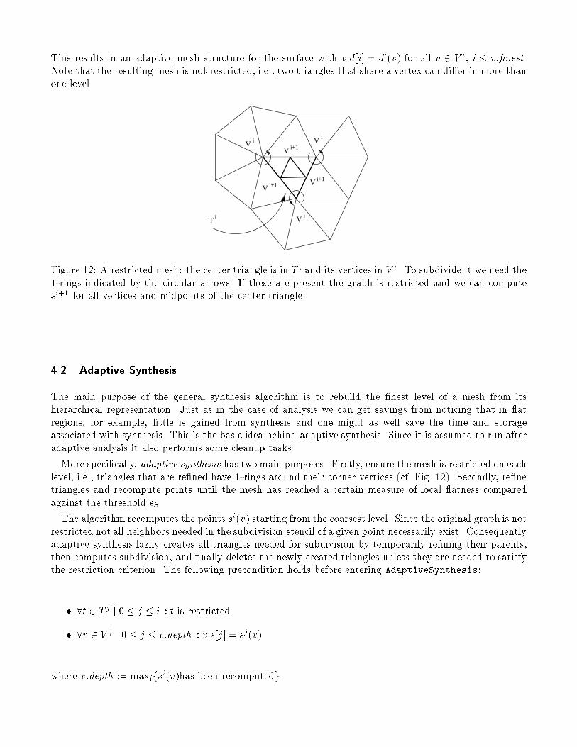
Figure 12: A restricted mesh: the center triangle is in T i and its vertices in V i. To subdivide it we need the1-rings indicated by the circular arrows. If these are present the graph is restricted and we can computesi+1 for all vertices and midpoints of the center triangle.
4.2 Adaptive Synthesis
The main purpose of the general synthesis algorithm is to rebuild the �nest level of a mesh from itshierarchical representation. Just as in the case of analysis we can get savings from noticing that in atregions, for example, little is gained from synthesis and one might as well save the time and storageassociated with synthesis. This is the basic idea behind adaptive synthesis. Since it is assumed to run afteradaptive analysis it also performs some cleanup tasks.
More speci�cally, adaptive synthesis has two main purposes. Firstly, ensure the mesh is restricted on eachlevel, i.e., triangles that are re�ned have 1-rings around their corner vertices (cf. Fig. 12). Secondly, re�netriangles and recompute points until the mesh has reached a certain measure of local atness comparedagainst the threshold �S .
The algorithm recomputes the points si(v) starting from the coarsest level. Since the original graph is notrestricted not all neighbors needed in the subdivision stencil of a given point necessarily exist. Consequentlyadaptive synthesis lazily creates all triangles needed for subdivision by temporarily re�ning their parents,then computes subdivision, and �nally deletes the newly created triangles unless they are needed to satisfythe restriction criterion. The following precondition holds before entering AdaptiveSynthesis:
� 8t 2 T j j 0 � j � i : t is restricted
� 8v 2 V j j 0 � j � v:depth : v:s[j] = sj(v)
where v:depth := maxifsi(v)has been recomputedg.
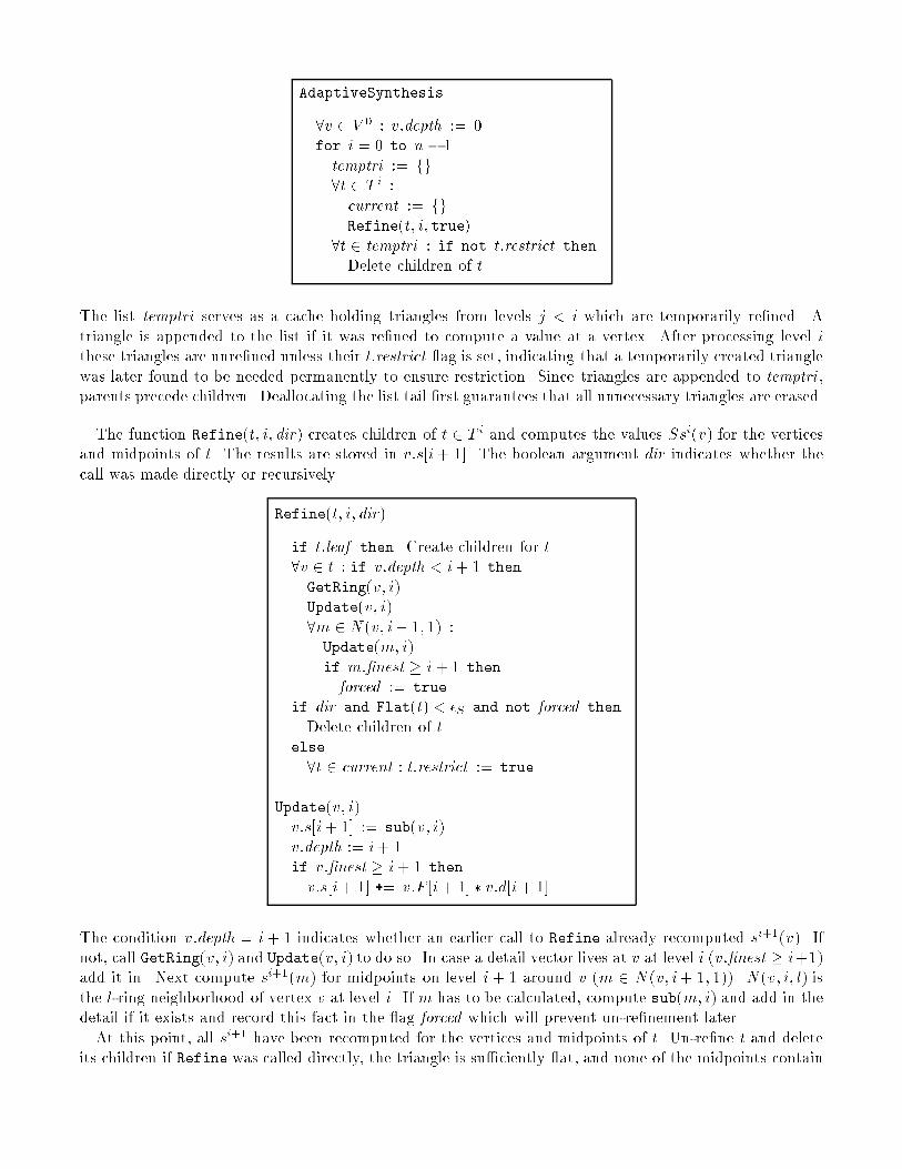
AdaptiveSynthesis
8v 2 V 0 : v:depth := 0for i = 0 to n � 1temptri := fg8t 2 T i :current := fgRefine(t; i; true)
8t 2 temptri : if not t:restrict then
Delete children of t
The list temptri serves as a cache holding triangles from levels j < i which are temporarily re�ned. Atriangle is appended to the list if it was re�ned to compute a value at a vertex. After processing level ithese triangles are unre�ned unless their t:restrict ag is set, indicating that a temporarily created trianglewas later found to be needed permanently to ensure restriction. Since triangles are appended to temptri ,parents precede children. Deallocating the list tail �rst guarantees that all unnecessary triangles are erased.
The function Refine(t; i; dir) creates children of t 2 T i and computes the values Ssi(v) for the verticesand midpoints of t. The results are stored in v:s[i+ 1]. The boolean argument dir indicates whether thecall was made directly or recursively
Refine(t; i; dir)
if t:leaf then Create children for t8v 2 t : if v:depth < i+ 1 then
GetRing(v; i)Update(v; i)8m 2 N(v; i+ 1; 1) :Update(m; i)if m:�nest � i+ 1 then
forced := true
if dir and Flat(t) < �S and not forced then
Delete children of telse
8t 2 current : t:restrict := true
Update(v; i)v:s[i+ 1] := sub(v; i)v:depth := i+ 1if v:�nest � i+ 1 then
v:s[i+ 1] += v:F [i+ 1] � v:d[i+ 1]
The condition v:depth = i+ 1 indicates whether an earlier call to Refine already recomputed si+1(v). Ifnot, call GetRing(v; i) and Update(v; i) to do so. In case a detail vector lives at v at level i (v:�nest � i+1)add it in. Next compute si+1(m) for midpoints on level i + 1 around v (m 2 N(v; i+ 1; 1)). N(v; i; l) isthe l-ring neighborhood of vertex v at level i. If m has to be calculated, compute sub(m; i) and add in thedetail if it exists and record this fact in the ag forced which will prevent un-re�nement later.
At this point, all si+1 have been recomputed for the vertices and midpoints of t. Un-re�ne t and deleteits children if Refine was called directly, the triangle is su�ciently at, and none of the midpoints contain
details (i.e. forced = false). The list current functions as a cache holding triangles from level i � 1which are temporarily re�ned to build a 1-ring around the vertices of t. If after processing all verticesand midpoints of t it is decided that t will remain re�ned, none of the level i � 1 triangles from currentcan be unre�ned without violating restriction. Thus t:restrict is set for all of them. The function Flat(t)measures how close to planar the corners and edge midpoints of t are.
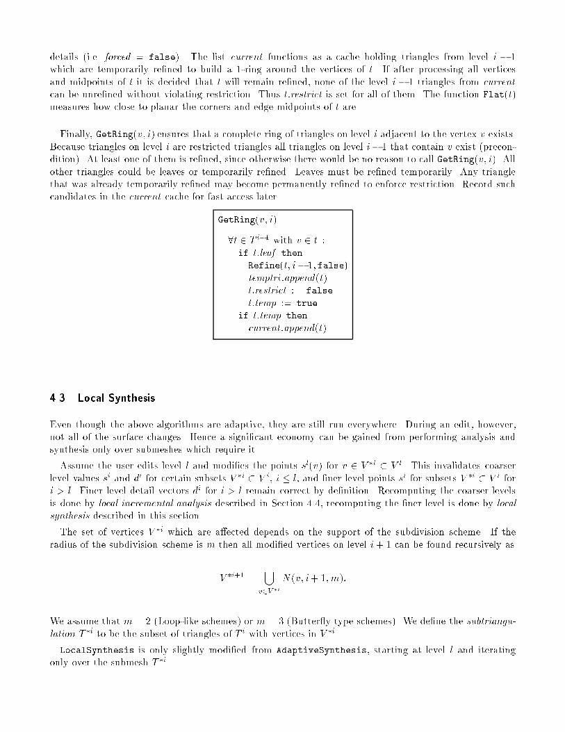
Finally, GetRing(v; i) ensures that a complete ring of triangles on level i adjacent to the vertex v exists.Because triangles on level i are restricted triangles all triangles on level i� 1 that contain v exist (precon-dition). At least one of them is re�ned, since otherwise there would be no reason to call GetRing(v; i). Allother triangles could be leaves or temporarily re�ned. Leaves must be re�ned temporarily. Any trianglethat was already temporarily re�ned may become permanently re�ned to enforce restriction. Record suchcandidates in the current cache for fast access later.
GetRing(v; i)
8t 2 T i�1 with v 2 t :if t:leaf then
Refine(t; i� 1; false)temptri :append(t)t:restrict := false
t:temp := true
if t:temp then
current :append(t)
4.3 Local Synthesis
Even though the above algorithms are adaptive, they are still run everywhere. During an edit, however,not all of the surface changes. Hence a signi�cant economy can be gained from performing analysis andsynthesis only over submeshes which require it.
Assume the user edits level l and modi�es the points sl(v) for v 2 V �l � V l. This invalidates coarserlevel values si and di for certain subsets V �i � V i, i � l, and �ner level points si for subsets V �i � V i fori > l. Finer level detail vectors di for i > l remain correct by de�nition. Recomputing the coarser levelsis done by local incremental analysis described in Section 4.4, recomputing the �ner level is done by localsynthesis described in this section.
The set of vertices V �i which are a�ected depends on the support of the subdivision scheme. If theradius of the subdivision scheme is m then all modi�ed vertices on level i+ 1 can be found recursively as
V �i+1 =[
v2V �i
N(v; i+ 1; m):
We assume that m = 2 (Loop-like schemes) or m = 3 (Butter y type schemes). We de�ne the subtriangu-lation T �i to be the subset of triangles of T i with vertices in V �i.
LocalSynthesis is only slightly modi�ed from AdaptiveSynthesis, starting at level l and iteratingonly over the submesh T �i
LocalSynthesis
8v 2 V �l : v:depth := lfor i = l to n � 1temptri := fg8t 2 T �i :current := fgRefine(t; i; true)
8t 2 temptri :if t:leaf and not t:restrict then
Delete children of t
4.4 Local Incremental Analysis
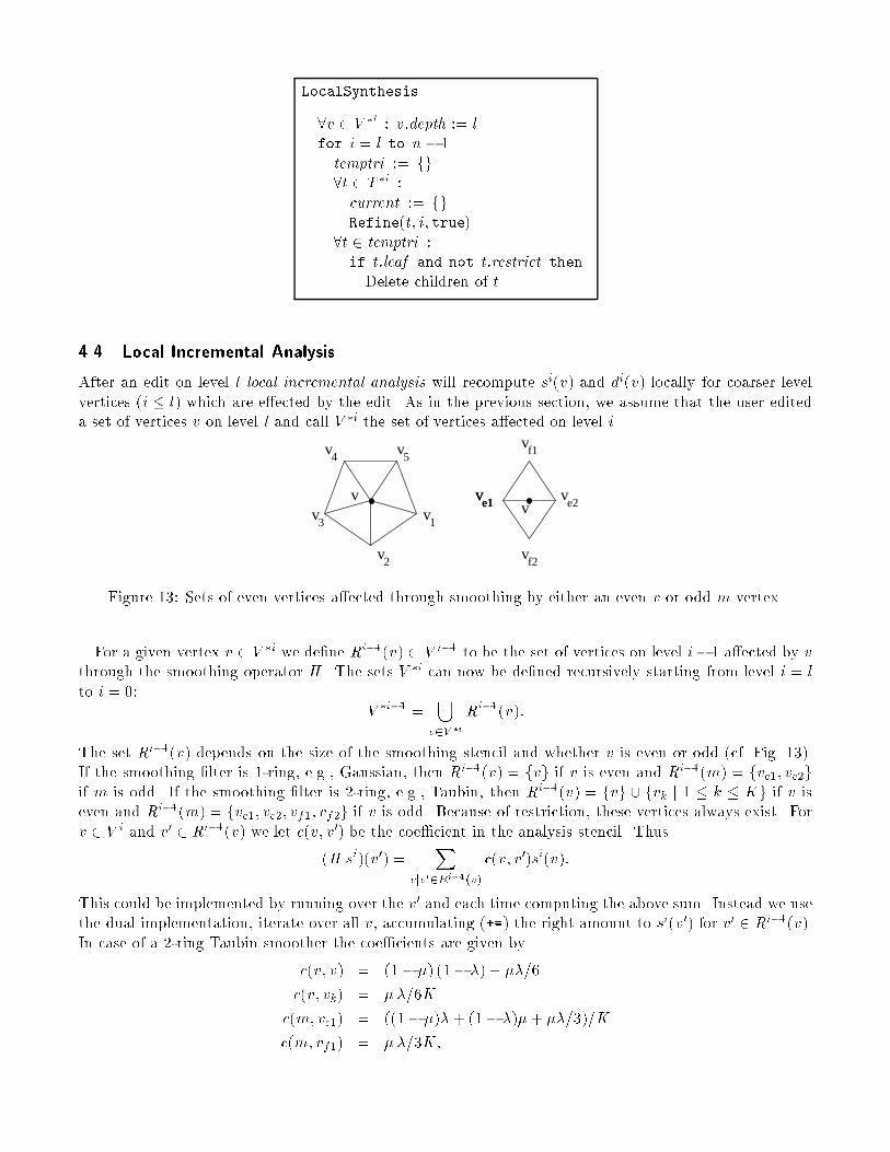
After an edit on level l local incremental analysis will recompute si(v) and di(v) locally for coarser levelvertices (i � l) which are e�ected by the edit. As in the previous section, we assume that the user editeda set of vertices v on level l and call V �i the set of vertices a�ected on level i.
1v
5v4v
vv
3
v e2v
vf2
f1v
e1v
2v
e1ve1v
Figure 13: Sets of even vertices a�ected through smoothing by either an even v or odd m vertex.
For a given vertex v 2 V �i we de�ne Ri�1(v) � V i�1 to be the set of vertices on level i� 1 a�ected by vthrough the smoothing operator H . The sets V �i can now be de�ned recursively starting from level i = l
to i = 0:V �i�1 =
[
v2V �i
Ri�1(v):
The set Ri�1(v) depends on the size of the smoothing stencil and whether v is even or odd (cf. Fig. 13).If the smoothing �lter is 1-ring, e.g., Gaussian, then Ri�1(v) = fvg if v is even and Ri�1(m) = fve1; ve2gif m is odd. If the smoothing �lter is 2-ring, e.g., Taubin, then Ri�1(v) = fvg [ fvk j 1 � k � Kg if v iseven and Ri�1(m) = fve1; ve2; vf1; vf2g if v is odd. Because of restriction, these vertices always exist. Forv 2 V i and v0 2 Ri�1(v) we let c(v; v0) be the coe�cient in the analysis stencil. Thus
(H si)(v0) =X
vjv02Ri�1(v)
c(v; v0)si(v):
This could be implemented by running over the v0 and each time computing the above sum. Instead we usethe dual implementation, iterate over all v, accumulating (+=) the right amount to si(v0) for v0 2 Ri�1(v).In case of a 2-ring Taubin smoother the coe�cients are given by
c(v; v) = (1� �) (1� �) + ��=6
c(v; vk) = ��=6K
c(m; ve1) = ((1� �)�+ (1� �)�+ ��=3)=K
c(m; vf1) = ��=3K;
where for each c(v; v0), K is the outdegree of v0.
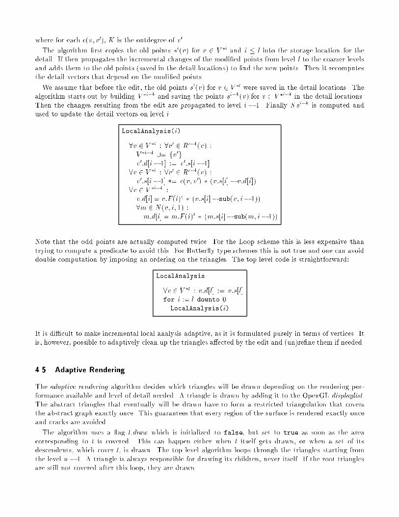
The algorithm �rst copies the old points si(v) for v 2 V �i and i � l into the storage location for thedetail. If then propagates the incremental changes of the modi�ed points from level l to the coarser levelsand adds them to the old points (saved in the detail locations) to �nd the new points. Then it recomputesthe detail vectors that depend on the modi�ed points.
We assume that before the edit, the old points sl(v) for v 2 V �l were saved in the detail locations. Thealgorithm starts out by building V �i�1 and saving the points si�1(v) for v 2 V �i�1 in the detail locations.Then the changes resulting from the edit are propagated to level i � 1. Finally S si�1 is computed andused to update the detail vectors on level i.
LocalAnalysis(i)
8v 2 V �i : 8v0 2 Ri�1(v) :V �i�1 [= fv0gv0:d[i� 1] := v0:s[i� 1]
8v 2 V �i : 8v0 2 Ri�1(v) :v0:s[i� 1] += c(v; v0) � (v:s[i]� v:d[i])
8v 2 V �i�1 :v:d[i] = v:F (i)t � (v:s[i]� sub(v; i� 1))8m 2 N(v; i; 1) :m:d[i] = m:F (i)t � (m:s[i]� sub(m; i� 1))
Note that the odd points are actually computed twice. For the Loop scheme this is less expensive thantrying to compute a predicate to avoid this. For Butter y type schemes this is not true and one can avoiddouble computation by imposing an ordering on the triangles. The top level code is straightforward:
LocalAnalysis
8v 2 V �l : v:d[l] := v:s[l]for i := l downto 0LocalAnalysis(i)
It is di�cult to make incremental local analysis adaptive, as it is formulated purely in terms of vertices. Itis, however, possible to adaptively clean up the triangles a�ected by the edit and (un)re�ne them if needed.
4.5 Adaptive Rendering
The adaptive rendering algorithm decides which triangles will be drawn depending on the rendering per-formance available and level of detail needed. A triangle is drawn by adding it to the OpenGL displaylist.The abstract triangles that eventually will be drawn have to form a restricted triangulation that coversthe abstract graph exactly once. This guarantees that every region of the surface is rendered exactly onceand cracks are avoided.
The algorithm uses a ag t:draw which is initialized to false, but set to true as soon as the areacorresponding to t is covered. This can happen either when t itself gets drawn, or when a set of itsdescendents, which cover t, is drawn. The top level algorithm loops through the triangles starting fromthe level n � 1. A triangle is always responsible for drawing its children, never itself. If the root trianglesare still not covered after this loop, they are drawn.
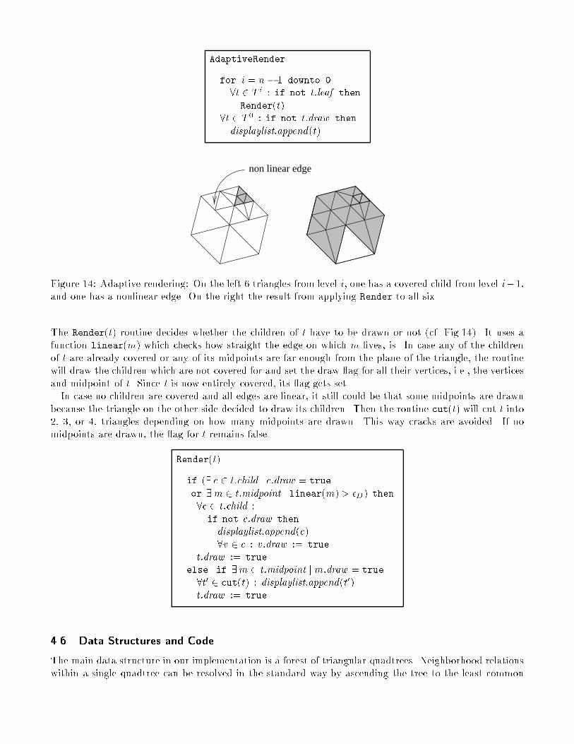
AdaptiveRender
for i = n � 1 downto 0
8t 2 T i : if not t:leaf then
Render(t)8t 2 T 0 : if not t:draw then
displaylist:append(t)
non linear edge
Figure 14: Adaptive rendering: On the left 6 triangles from level i, one has a covered child from level i+1,and one has a nonlinear edge. On the right the result from applying Render to all six.
The Render(t) routine decides whether the children of t have to be drawn or not (cf. Fig.14). It uses afunction linear(m) which checks how straight the edge on which m lives, is. In case any of the childrenof t are already covered or any of its midpoints are far enough from the plane of the triangle, the routinewill draw the children which are not covered for and set the draw ag for all their vertices, i.e., the verticesand midpoint of t. Since t is now entirely covered, its ag gets set.In case no children are covered and all edges are linear, it still could be that some midpoints are drawn
because the triangle on the other side decided to draw its children. Then the routine cut(t) will cut t into2, 3, or 4, triangles depending on how many midpoints are drawn. This way cracks are avoided. If nomidpoints are drawn, the ag for t remains false.
Render(t)
if (9 c 2 t:child j c:draw = true
or 9m 2 t:midpoint j linear(m) > �D) then
8c 2 t:child :if not c:draw then
displaylist:append(c)8v 2 c : v:draw := true
t:draw := true
else if 9m 2 t:midpoint jm:draw = true
8t0 2 cut(t) : displaylist:append(t0)t:draw := true
4.6 Data Structures and Code
The main data structure in our implementation is a forest of triangular quadtrees. Neighborhood relationswithin a single quadtree can be resolved in the standard way by ascending the tree to the least common
parent when attempting to �nd the neighbor across a given edge. Neighbor relations between adjacenttrees are resolved explicitly at the level of a collection of roots, i.e., faces of a coarsest level graph. Thisstructure also maintains an explicit representation of the boundary (if any). Submeshes rooted at anylevel can be created on the y by assembling a new graph with some set of triangles as roots of their childquadtrees. It is here that the explicit representation of the boundary comes in, since the actual trees arenever copied, and a boundary is needed to delineate the actual submesh.
The algorithms we have described above make heavy use of container classes. E�cient support forsets is essential for a fast implementation and we have used the C++ Standard Template Library. Themesh editor was implemented using OpenInventor and OpenGL and currently runs on both SGI and IntelPentiumPro workstations.
5 Results
In this section we show some example images to demonstrate various features of our system and giveperformance measures.
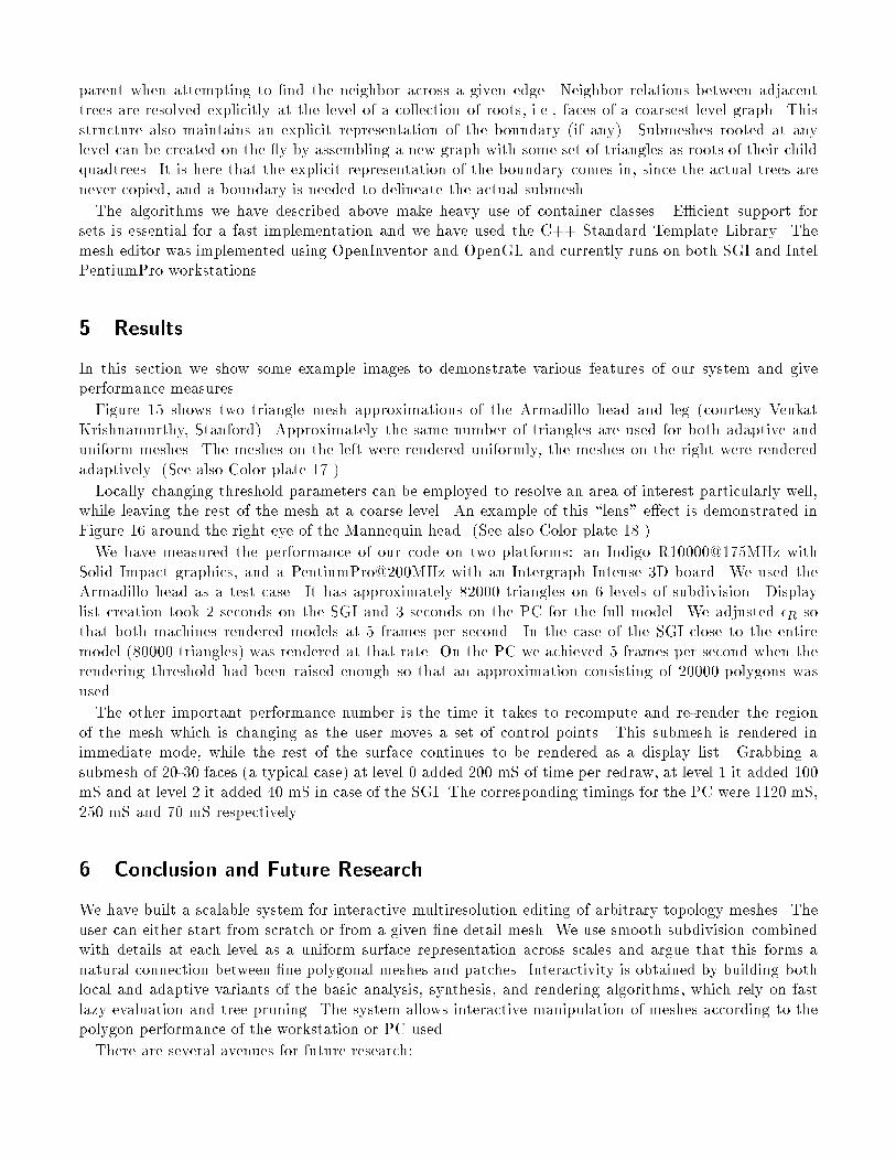
Figure 15 shows two triangle mesh approximations of the Armadillo head and leg (courtesy VenkatKrishnamurthy, Stanford). Approximately the same number of triangles are used for both adaptive anduniform meshes. The meshes on the left were rendered uniformly, the meshes on the right were renderedadaptively. (See also Color plate 17.)
Locally changing threshold parameters can be employed to resolve an area of interest particularly well,while leaving the rest of the mesh at a coarse level. An example of this \lens" e�ect is demonstrated inFigure 16 around the right eye of the Mannequin head. (See also Color plate 18.)
We have measured the performance of our code on two platforms: an Indigo R10000@175MHz withSolid Impact graphics, and a PentiumPro@200MHz with an Intergraph Intense 3D board. We used theArmadillo head as a test case. It has approximately 82000 triangles on 6 levels of subdivision. Displaylist creation took 2 seconds on the SGI and 3 seconds on the PC for the full model. We adjusted �R sothat both machines rendered models at 5 frames per second. In the case of the SGI close to the entiremodel (80000 triangles) was rendered at that rate. On the PC we achieved 5 frames per second when therendering threshold had been raised enough so that an approximation consisting of 20000 polygons wasused.
The other important performance number is the time it takes to recompute and re-render the regionof the mesh which is changing as the user moves a set of control points. This submesh is rendered inimmediate mode, while the rest of the surface continues to be rendered as a display list. Grabbing asubmesh of 20-30 faces (a typical case) at level 0 added 200 mS of time per redraw, at level 1 it added 100mS and at level 2 it added 40 mS in case of the SGI. The corresponding timings for the PC were 1120 mS,250 mS and 70 mS respectively.
6 Conclusion and Future Research
We have built a scalable system for interactive multiresolution editing of arbitrary topology meshes. Theuser can either start from scratch or from a given �ne detail mesh. We use smooth subdivision combinedwith details at each level as a uniform surface representation across scales and argue that this forms anatural connection between �ne polygonal meshes and patches. Interactivity is obtained by building bothlocal and adaptive variants of the basic analysis, synthesis, and rendering algorithms, which rely on fastlazy evaluation and tree pruning. The system allows interactive manipulation of meshes according to thepolygon performance of the workstation or PC used.
There are several avenues for future research:
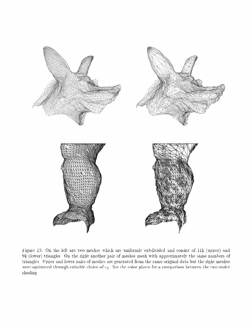
Figure 15: On the left are two meshes which are uniformly subdivided and consist of 11k (upper) and9k (lower) triangles. On the right another pair of meshes mesh with approximately the same numbers oftriangles. Upper and lower pairs of meshes are generated from the same original data but the right mesheswere optimized through suitable choice of �S . See the color plates for a comparison between the two undershading.
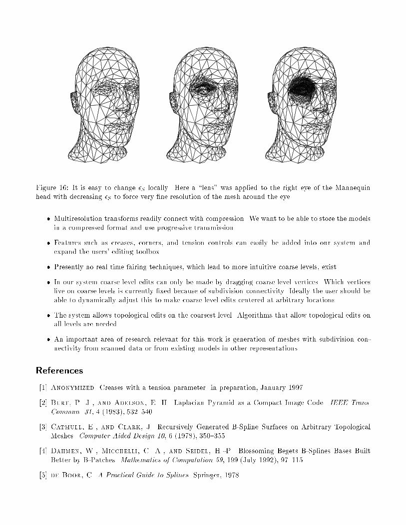
Figure 16: It is easy to change �S locally. Here a \lens" was applied to the right eye of the Mannequinhead with decreasing �S to force very �ne resolution of the mesh around the eye.
� Multiresolution transforms readily connect with compression. We want to be able to store the modelsin a compressed format and use progressive transmission.
� Features such as creases, corners, and tension controls can easily be added into our system andexpand the users' editing toolbox.
� Presently no real time fairing techniques, which lead to more intuitive coarse levels, exist.
� In our system coarse level edits can only be made by dragging coarse level vertices. Which verticeslive on coarse levels is currently �xed because of subdivision connectivity. Ideally the user should beable to dynamically adjust this to make coarse level edits centered at arbitrary locations.
� The system allows topological edits on the coarsest level. Algorithms that allow topological edits onall levels are needed.
� An important area of research relevant for this work is generation of meshes with subdivision con-nectivity from scanned data or from existing models in other representations.
References
[1] Anonymized. Creases with a tension parameter. in preparation, January 1997.
[2] Burt, P. J., and Adelson, E. H. Laplacian Pyramid as a Compact Image Code. IEEE Trans.Commun. 31, 4 (1983), 532{540.
[3] Catmull, E., and Clark, J. Recursively Generated B-Spline Surfaces on Arbitrary TopologicalMeshes. Computer Aided Design 10, 6 (1978), 350{355.
[4] Dahmen, W., Micchelli, C. A., and Seidel, H.-P. Blossoming Begets B-Splines Bases BuiltBetter by B-Patches. Mathematics of Computation 59, 199 (July 1992), 97{115.
[5] de Boor, C. A Practical Guide to Splines. Springer, 1978.
[6] Doo, D., and Sabin, M. Analysis of the Behaviour of Recursive Division Surfaces near ExtraordinaryPoints. Computer Aided Design 10, 6 (1978), 356{360.
[7] Dyn, N., Levin, D., and Gregory, J. A. A Butter y Subdivision Scheme for Surface Interpolationwith Tension Control. ACM Trans. Gr. 9, 2 (April 1990), 160{169.
[8] Eck, M., DeRose, T., Duchamp, T., Hoppe, H., Lounsbery, M., and Stuetzle, W. Mul-tiresolution Analysis of Arbitrary Meshes. Computer Graphics Proceedings, (SIGGRAPH 95) (1995),173{182.
[9] Eck, M., DeRose, T., Duchamp, T., Hoppe, H., Lounsbery, M., and Stuetzle, W. Multires-olution Analysis of Arbitrary Meshes. In Computer Graphics Proceedings, Annual Conference Series,173{182, 1995.
[10] Finkelstein, A., and Salesin, D. H. Multiresolution Curves. Computer Graphics Proceedings,Annual Conference Series, 261{268, July 1994.
[11] Forsey, D., and Wong, D. Multiresolution Surface Reconstruction for Hierarchical B-splines. Tech.rep., University of British Columbia, 1995.
[12] Forsey, D. R., and Bartels, R. H. Hierarchical B-Spline Re�nement. Computer Graphics (SIG-GRAPH '88 Proceedings), Vol. 22, No. 4, pp. 205{212, August 1988.
[13] Gortler, S. J., and Cohen, M. F. Hierarchical and Variational Geometric Modeling with Wavelets.In Proceedings Symposium on Interactive 3D Graphics, May 1995.
[14] Hoppe, H. Progressive Meshes. In SIGGRAPH 96 Conference Proceedings, H. Rushmeier, Ed.,Annual Conference Series, 99{108, August 1996.
[15] Hoppe, H., DeRose, T., Duchamp, T., Halstead, M., Jin, H., McDonald, J., Schweitzer,J., and Stuetzle, W. Piecewise Smooth Surface Reconsruction. In Computer Graphics Proceedings,Annual Conference Series, 295{302, 1994.
[16] Hoppe, H., DeRose, T., Duchamp, T., McDonald, J., and Stuetzle, W. Mesh Optimization.In Computer Graphics (SIGGRAPH '93 Proceedings), J. T. Kajiya, Ed., vol. 27, 19{26, August 1993.
[17] Kobbelt, L. Interpolatory Subdivision on Open Quadrilateral Nets with Arbitrary Topology. InProceedings of Eurographics 96, Computer Graphics Forum, 409{420, 1996.
[18] Krishnamurthy, V., and Levoy, M. Fitting Smooth Surfaces to Dense Polygon Meshes. In SIG-GRAPH 96 Conference Proceedings, H. Rushmeier, Ed., Annual Conference Series, 313{324, August1996.
[19] Kurihara, T. Interactive Surface Design Using Recursive Subdivision. In Proceedings of Communi-cating with Virtual Worlds. Springer Verlag, June 1993.
[20] Loop, C. Smooth Subdivision Surfaces Based on Triangles. Master's thesis, University of Utah,Department of Mathematics, 1987.
[21] Loop, C. Smooth Spline Surfaces over Irregular Meshes. In Computer Graphics Proceedings, AnnualConference Series, 303{310, 1994.
[22] Lounsbery, M., DeRose, T. D., and Warren, J. Multiresolution Surfaces of Arbitrary Topo-logical Type. Department of Computer Science and Engineering 93-10-05, University of Washington,October 1993. Updated version available as 93-10-05b, January, 1994.
[23] Peters, J. C1 Surface Splines. SIAM J. Numer. Anal. 32, 2 (1995), 645{666.
[24] Schr�oder, P., and Sweldens, W. Spherical wavelets: E�ciently representing functions on thesphere. Computer Graphics Proceedings, (SIGGRAPH 95) (1995), 161{172.
[25] Schweitzer, J. E. Analysis and Application of Subdivision Surfaces. PhD thesis, University ofWashington, 1996.
[26] Taubin, G. A Signal Processing Approach to Fair Surface Design. In SIGGRAPH 95 ConferenceProceedings, R. Cook, Ed., Annual Conference Series, 351{358, August 1995.
[27] Zorin, D., Schr�oder, P., and Sweldens, W. Interpolating Subdivision for Meshes with ArbitraryTopology. Computer Graphics Proceedings (SIGGRAPH 96) (1996), 189{192.
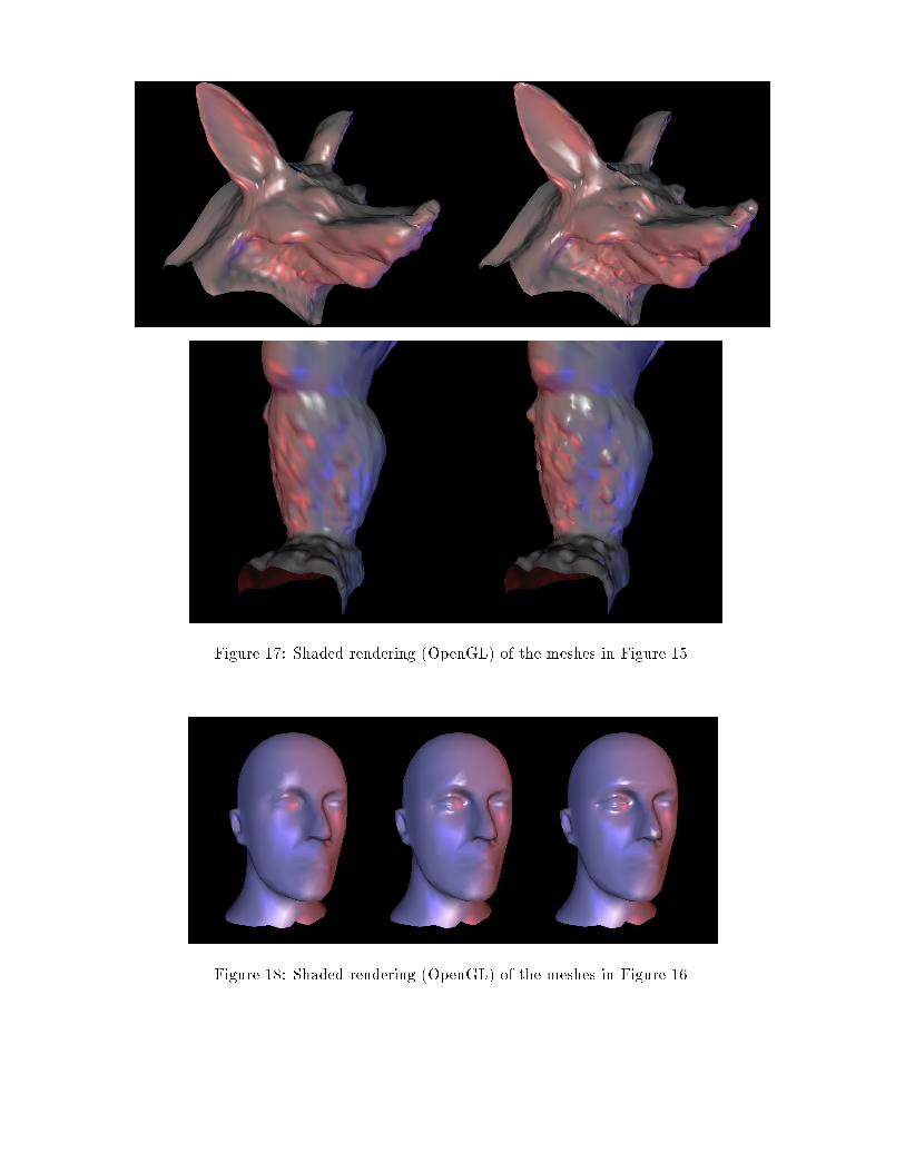
Figure 17: Shaded rendering (OpenGL) of the meshes in Figure 15.
Figure 18: Shaded rendering (OpenGL) of the meshes in Figure 16.