International Institute for Tel: 43 2236 807 342Applied Systems Analysis Fax: 43 2236 71313Schlossplatz 1 E-mail: publications@iiasa.ac.atA-2361 Laxenburg, Austria Web: www.iiasa.ac.at

Interim Report IR-09-020

Interactive Fuzzy Random Two-level Linear ProgrammingThrough Fractile Criterion OptimizationMasatoshi Sakawa (sakawa@hiroshima-u.ac.jp)Kosuke Kato(kosuke-kato@hiroshima-u.ac.jp)

Approved by

Marek Makowski (marek@iiasa.ac.at)Leader, Integrated Modeling Environment Project

May 2009

Interim Reports on work of the International Institute for Applied Systems Analysis receive only limitedreview. Views or opinions expressed herein do not necessarily represent those of the Institute, its NationalMember Organizations, or other organizations supporting the work.

– ii –

Foreword

In this paper, assuming cooperative behavior of the decision makers, we consider solutionmethods for decision making problems in hierarchical organizations under fuzzy randomenvironments. To deal with the formulated two-level linear programming problems in-volving fuzzy random variables,α-level sets of fuzzy random variables are introducedand anα-stochastic two-level linear programming problem is defined for guaranteeingthe degree of realization of the problem. Taking into account vagueness of judgmentsof decision makers, fuzzy goals are introduced and theα-stochastic two-level linear pro-gramming problem is transformed into the problem to maximize the satisfaction degreefor each fuzzy goal. Through the use of the fractile criterion optimization model, thetransformed stochastic two-level programming problem can be reduced to a determinis-tic one. Interactive fuzzy programming to obtain a satisfactory solution for the decisionmaker at the upper level in consideration of the cooperative relation between decisionmakers is presented. It is significant to note here that all of the problems to be solved inthe proposed interactive fuzzy programming can be easily solved by the simplex method,the sequential quadratic programming or the combined use of the bisection method andthe sequential quadratic programming. An illustrative numerical example is provided todemonstrate the feasibility and efficiency of the proposed method.

– iii –

Abstract

This paper considers two-level linear programming problems involving fuzzy randomvariables. Having introduced level sets of fuzzy random variables and fuzzy goals of de-cision makers, following fractile criterion optimization, fuzzy random two-level program-ming problems are transformed into deterministic ones. Interactive fuzzy programmingis presented for deriving a satisfactory solution efficiently with considerations of overallsatisfactory balance.

Keywords: Fuzzy programming; fuzzy random variables; interactive decision making;two-level linear programming problems; fractile criterion optimization; level sets.

– iv –

Acknowledgments

Masatoshi Sakawa appreciates the hospitality and the working environment during histwo-months Guest Scholar affiliation with the Integrated Modeling Project. The researchpresented in this paper was completed and the paper written during this time.

– v –

About the Authors

Masatoshi Sakawa joined the Integrated Modeling Environment in April 2009. His re-search and teaching activities are in the area of systems engineering, especially mathe-matical optimization, multiobjective decision making, fuzzy mathematical programmingand game theory. In addition to over 300 articles in national and international journals,he is an author and coauthor of 5 books in English and 14 books in Japanese. At presentDr. Sakawa is a Professor at Hiroshima University, Japan and is working with the Depart-ment of Artificial Complex Systems Engineering. Dr. Sakawa received BEng, MEng, andDEng degrees in applied mathematics and physics at Kyoto University, in 1970, 1972,and 1975 respectively. From 1975 he was with Kobe University, where from 1981 hewas an Associate Professor in the Department of Systems Engineering. From 1987 to1990 he was Professor of the Department of Computer Science at Iwate University andfrom March to December 1991 he was an Honorary Visiting Professor at the Universityof Manchester Institute of Science and Technology (UMIST), Computation Department,sponsored by the Japan Society for the Promotion of Science (JSPS). He was also a Visit-ing Professor of the Institute of Economic Research, Kyoto University from April 1991 toMarch 1992. In 2002 Dr. Sakawa received the Georg Cantor Award of the InternationalSociety on Multiple Criteria Decision Making.

Kosuke Kato is an Associate Professor at Department of Artificial Complex SystemsEngineering, Hiroshima University, Japan. He received B.E. and M.E. degrees in bio-physical engineering from Osaka University, in 1991 and 1993, respectively. He receivedD.E. degree from Kyoto University in 1999. His current research interests are evolution-ary computation, large-scale programming and multiobjective/multi-level programmingunder uncertain environments.

– vi –

Contents

1 Introduction 1

2 Fuzzy random two-level linear programming problems 2

3 Level Sets and fuzzy goals 4

4 Fractile criterion optimization 6

5 Interactive fuzzy programming 9

6 Numerical example 12

7 Conclusions 14

– 1 –

Interactive Fuzzy Random Two-level LinearProgramming Through Fractile Criterion Optimization

Masatoshi Sakawa (sakawa@hiroshima-u.ac.jp)* **

Kosuke Kato(kosuke-kato@hiroshima-u.ac.jp)*

1 Introduction

Fuzzy random variables, first introduced by Kwakernaak [16], have been developing invarious ways [15, 27, 21]. An overview of the developments of fuzzy random variableswas found in the article of Gil, Lopez-Diaz and Ralescu [7]. Studies on linear program-ming problems with fuzzy random variable coefficients, called fuzzy random linear pro-gramming problems, were initiated by Wang and Qiao [45], Qaio, Zhang and Wang [28]as seeking the probability distribution of the optimal solution and optimal value. Opti-mization models for fuzzy random linear programming problems were first considered byLuhandjula et al. [22, 24] and further developed by Liu [19, 20] and Rommelfanger [30].A brief survey of major fuzzy stochastic programming models was found in the paperby Luhandjula [23]. As we look at recent developments in the fields of fuzzy randomprogramming, we can see continuing advances [9, 12, 10, 11, 14, 30, 13, 2, 47].

However, decision making problems in hierarchical managerial or public organiza-tions are often formulated as two-level mathematical programming problems [34]. In thecontext of two-level programming, the decision maker at the upper level first specifies astrategy, and then the decision maker at the lower level specifies a strategy so as to opti-mize the objective with full knowledge of the action of the decision maker at the upperlevel. In conventional multi-level mathematical programming models employing the so-lution concept of Stackelberg equilibrium, it is assumed that there is no communicationamong decision makers, or they do not make any binding agreement even if there existssuch communication [41, 3, 40, 25] . Compared with this, for decision making problemsin such as decentralized large firms with divisional independence, it is quite natural tosuppose that there exists communication and some cooperative relationship among thedecision makers [34].

Lai [17] and Shih et al. [39] proposed solution concepts for two-level linear program-ming problems or multi-level ones such that decisions of decision makers in all levels aresequential and all of the decision makers essentially cooperate with each other. In theirmethods, the decision makers identify membership functions of the fuzzy goals for theirobjective functions, and in particular, the decision maker at the upper level also speci-fies those of the fuzzy goals for the decision variables. The decision maker at the lower

* Graduate School of Engineering, Hiroshima University.** Corresponding author.

– 2 –

level solves a fuzzy programming problem with a constraint with respect to a satisfactorydegree of the decision maker at the upper level. Unfortunately, there is a possibility thattheir method leads a final solution to an undesirable one because of inconsistency betweenthe fuzzy goals of the objective function and those of the decision variables. In order toovercome the problem in their methods, by eliminating the fuzzy goals for the decisionvariables, Sakawa et al. have proposed interactive fuzzy programming for two-level ormulti-level linear programming problems to obtain a satisfactory solution for decisionmakers [35, 36]. The subsequent works on two-level or multi-level programming havebeen appearing [18, 32, 33, 37, 38, 42, 26, 1, 29, 34].

Under these circumstances, in this paper, assuming cooperative behavior of the deci-sion makers, we consider solution methods for decision making problems in hierarchicalorganizations under fuzzy random environments. To deal with the formulated two-levellinear programming problems involving fuzzy random variables,α-level sets of fuzzyrandom variables are introduced and anα-stochastic two-level linear programming prob-lem is defined for guaranteeing the degree of realization of the problem. Taking intoaccount vagueness of judgments of decision makers, fuzzy goals are introduced and theα-stochastic two-level linear programming problem is transformed into the problem tomaximize the satisfaction degree for each fuzzy goal. Following the fractile criterion op-timization model [8], the transformed stochastic two-level programming problem can bereduced to a deterministic one. Interactive fuzzy programming to obtain a satisfactory so-lution for the decision maker at the upper level in consideration of the cooperative relationbetween decision makers is presented. It is shown that all of the problems to be solved inthe proposed interactive fuzzy programming can be easily solved by the simplex method,the sequential quadratic programming or the combined use of the bisection method andthe sequential quadratic programming. An illustrative numerical example is provided todemonstrate the feasibility and efficiency of the proposed method.

2 Fuzzy random two-level linear programming problems

Fuzzy random variables, first introduced by Kwakernaak [16], have been defined in vari-ous ways [16, 27, 15, 21]. For example, as a special case of fuzzy random variables givenby Kwakernaak, Kruse and Meyer [15] defined a fuzzy random variable as follows.

Definition 1 (Fuzzy random variable) Let (Ω, B, P ) be a probability space,F (R) theset of fuzzy numbers with compact supports andX a measurable mappingΩ → F (R).ThenX is a fuzzy random variable if and only if givenω ∈ Ω,Xα(ω) is a random intervalfor anyα ∈ (0, 1], whereXα(ω) is anα-level set of the fuzzy setX(ω).

Although there exist some minor differences in several definitions of fuzzy random vari-ables, fuzzy random variables are considered to be random variables whose observedvalues are fuzzy sets.

– 3 –

In this paper, we deal with two-level linear programming problems involving fuzzyrandom variable coefficients in objective functions formulated as:

minimizefor DM1

z1(x1,x2) = ˜C11x1 + ˜C12x2

minimizefor DM2

z2(x1,x2) = ˜C21x1 + ˜C22x2

subject toA1x1 +A2x2 ≤ bx1 ≥ 0 , x2 ≥ 0

. (1)

It should be emphasized here that randomness and fuzziness of the coefficients aredenoted by the “dash above” and “wave above” i.e.,“¯” and“˜ ”, respectively. In (1),x1 is ann1 dimensional decision variable column vector for the decision maker at theupper level (DM1), x2 is ann2 dimensional decision variable column vector for the de-cision maker at the lower level (DM2), z1(x1,x2) is the objective function for DM1 andz2(x1,x2) is the objective function for DM2. Elements˜Cljk, k = 1, 2, . . . , nj of coef-

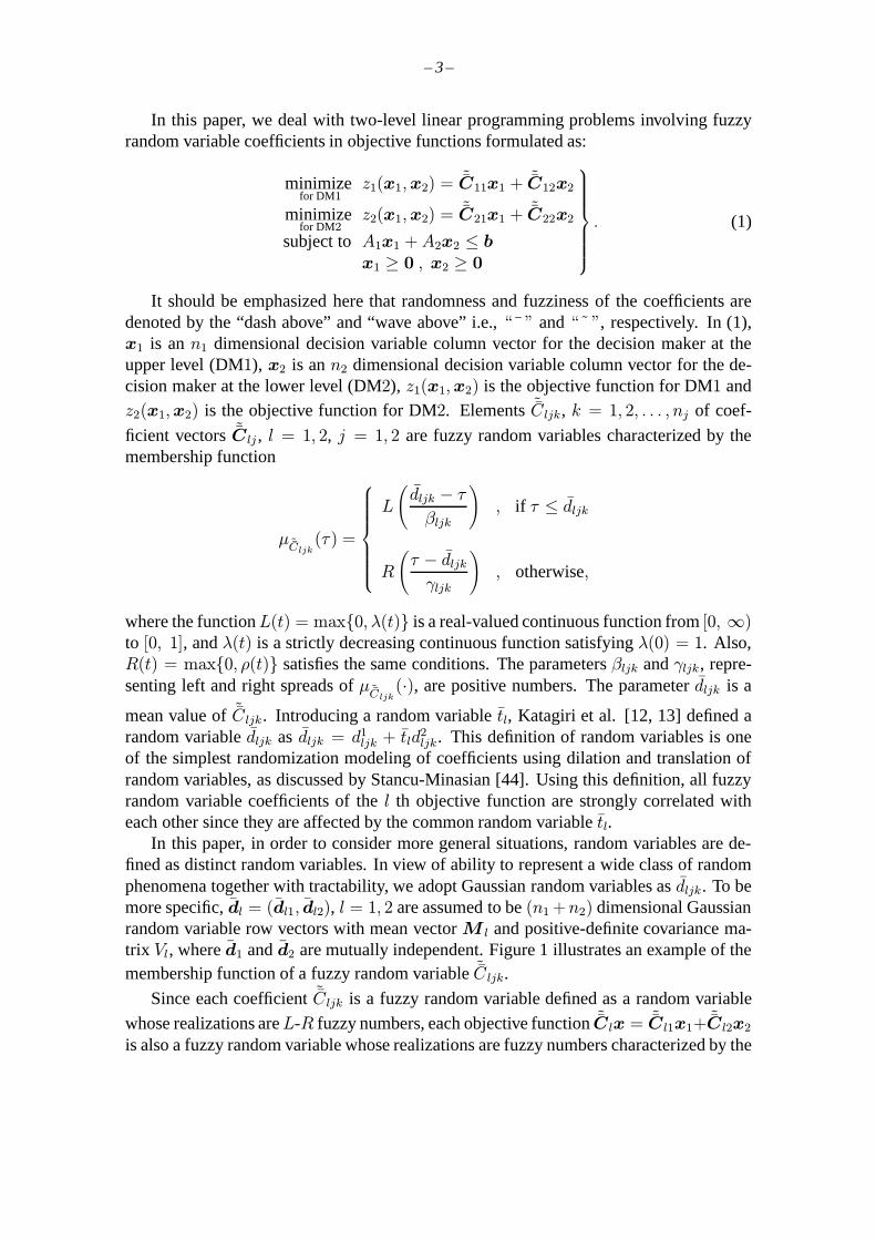
ficient vectors˜Clj , l = 1, 2, j = 1, 2 are fuzzy random variables characterized by themembership function

µ ˜Cljk(τ ) =

L

(dljk − τβljk

), if τ ≤ dljk

R

(τ − dljkγljk

), otherwise,

where the functionL(t) = max0, λ(t) is a real-valued continuous function from[0, ∞)to [0, 1], andλ(t) is a strictly decreasing continuous function satisfyingλ(0) = 1. Also,R(t) = max0, ρ(t) satisfies the same conditions. The parametersβljk andγljk, repre-senting left and right spreads ofµ ˜Cljk

(·), are positive numbers. The parameterdljk is a

mean value ofCljk. Introducing a random variabletl, Katagiri et al. [12, 13] defined arandom variabledljk as dljk = d1

ljk + tld2ljk. This definition of random variables is one

of the simplest randomization modeling of coefficients using dilation and translation ofrandom variables, as discussed by Stancu-Minasian [44]. Using this definition, all fuzzyrandom variable coefficients of thel th objective function are strongly correlated witheach other since they are affected by the common random variabletl.

In this paper, in order to consider more general situations, random variables are de-fined as distinct random variables. In view of ability to represent a wide class of randomphenomena together with tractability, we adopt Gaussian random variables asdljk. To bemore specific,dl = (dl1, dl2), l = 1, 2 are assumed to be(n1 +n2) dimensional Gaussianrandom variable row vectors with mean vectorM l and positive-definite covariance ma-trix Vl, whered1 andd2 are mutually independent. Figure 1 illustrates an example of themembership function of a fuzzy random variable˜C ljk.

Since each coefficientCljk is a fuzzy random variable defined as a random variable

whose realizations areL-R fuzzy numbers, each objective function˜Clx = ˜Cl1x1+ ˜Cl2x2

is also a fuzzy random variable whose realizations are fuzzy numbers characterized by the

– 4 –

Figure 1: An example of the membership functionµ ˜Cljk(·) of a fuzzy random variable

˜C ljk.

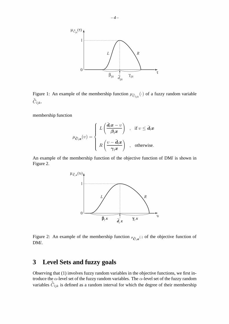
membership function

µ ˜C lx(υ) =

L

(dlx− υβlx

), if υ ≤ dlx

R

(υ − dlxγ lx

), otherwise.

An example of the membership function of the objective function of DMl is shown inFigure 2.

Figure 2: An example of the membership functionµ ˜Clx(·) of the objective function of

DMl.

3 Level Sets and fuzzy goals

Observing that (1) involves fuzzy random variables in the objective functions, we first in-troduce theα-level set of the fuzzy random variables. Theα-level set of the fuzzy randomvariables˜Cljk is defined as a random interval for which the degree of their membership

– 5 –

functions exceeds the levelα:

˜C ljkα = τ | µ ˜Cljk(τ ) ≥ α, τ ∈ R, j = 1, 2, k = 1, 2, . . . , nj.

For notational convenience, in the following, let˜Clα = ( ˜C l1α,˜Cl2α), l = 1, 2 be anα-

level set defined as the Cartesian product ofα-level sets˜Cljkα of fuzzy random variables˜C ljk, j = 1, 2, k = 1, 2, . . . , nj.

Now suppose that DM1 decides that the degree of all of the membership functionsof the fuzzy random variables involved in (1) should be greater than or equal to somevalueα. Then for such a degreeα, (1) can be interpreted as the following stochastic two-level linear programming problem which depends on the coefficient vectors(C11, C12) ∈( ˜C11α,

˜C12α) and(C21, C22) ∈ ( ˜C21α,˜C22α):

minimizefor DM1

z1(x1,x2) = C11x1 + C12x2

minimizefor DM2

z2(x1,x2) = C21x1 + C22x2

subject toA1x1 +A2x2 ≤ bx1 ≥ 0, x2 ≥ 0

. (2)

Observe that there exists an infinite number of such problems depending on the coeffi-cient vector(C11, C12) ∈ ( ˜C11α,

˜C12α) and (C21, C22) ∈ ( ˜C21α,˜C22α), and the val-

ues of(C11, C12) and(C21, C22) are arbitrary for any(C11, C12) ∈ ( ˜C11α,˜C12α) and

(C21, C22) ∈ ( ˜C21α,˜C22α) in the sense that the degree of all of the membership functions

for the fuzzy random variables in (2) exceeds the levelα. However, if possible, it would bedesirable for DM1 to choose(C11, C12) ∈ ( ˜C11α,

˜C12α) and(C21, C22) ∈ ( ˜C21α,˜C22α)

in (2) to minimize the objective functions under the constraints. From such a point ofview, for a certain degreeα, it seems to be quite natural to have (2) reformulated as thefollowing α-stochastic two-level linear programming problem:

minimizefor DM1

z1(x1,x2) = C11x1 + C12x2

minimizefor DM2

z2(x1,x2) = C21x1 + C22x2

subject toA1x1 +A2x2 ≤ bx1 ≥ 0, x2 ≥ 0C1 = (C11, C12) ∈ ˜C1α, C2 = (C21, C22) ∈ ˜C2α

. (3)

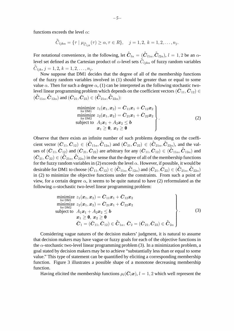
Considering vague natures of the decision makers’ judgment, it is natural to assumethat decision makers may have vague or fuzzy goals for each of the objective functions intheα-stochastic two-level linear programming problem (3). In a minimization problem, agoal stated by decision makers may be to achieve “substantially less than or equal to somevalue.” This type of statement can be quantified by eliciting a corresponding membershipfunction. Figure 3 illustrates a possible shape of a monotone decreasing membershipfunction.

Having elicited the membership functionsµl(Clx), l = 1, 2 which well represent the

– 6 –

Figure 3: An example of a membership functionµl(·) of a fuzzy goal.

fuzzy goals of the decision makers at both levels, problem (3) can be transformed as:

maximizefor DM1

µ1(C1x)

maximizefor DM2

µ2(C2x)

subject toA1x1 +A2x2 ≤ bx1 ≥ 0, x2 ≥ 0C1 ∈ ˜C1α, C2 ∈ ˜C2α

. (4)

ObservingClx andµl(Clx) involve random variables, it is significant to note here (4) isa stochastic programming problem.

4 Fractile criterion optimization

Since (4) contains random variable coefficients, solution methods for ordinary determin-istic two-level linear programming problems cannot be directly applied. In stochasticprogramming, expectation optimization, variance minimization, probability maximiza-tion and fractile criterion optimization [5, 6, 8, 43, 46, 4] are typical optimization modelsfor objective functions involving random variables. For instance, let the objective functionrepresent a profit. If the decision maker wishes to simply maximize the expected profitwithout caring about the fluctuation of the profit, the expectation optimization model [6]to optimize the expectation of the objective function is appropriate. On the other hand,if the decision maker hopes to decrease the fluctuation of the profit as little as possiblefrom the viewpoint of the stability of the profit, the variance minimization model [6] tominimize the variance of the objective function is useful. In contrast to these two typesof optimizing approaches, as satisficing approaches, the probability maximization model[6] and the fractile criterion optimization model or Kataoka’s model [8] have been pro-posed. When the decision maker wants to maximize the probability that the profit isgreater than or equal to a certain permissible level, probability maximization model [6] isrecommended. In contrast, when the decision maker wishes to optimize such a permissi-ble level as the probability that the profit is greater than or equal to the permissible level isgreater than or equal to a certain threshold, the fractile criterion optimization model willbe appropriate.

In this paper, assuming that the decision makers are interested in the probability thateach objective function attains a goal value rather than the expectation or variance of each

– 7 –

membership function, we adopt the fractile criterion optimization model [8] as a decisionmaking model. Through fractile criterion optimization, problem (4) can be rewritten as:

maximizefor DM1

h1

maximizefor DM2

h2

subject to Prµ1(C1x) ≥ h1

≥ θ1

Prµ2(C2x) ≥ h2

≥ θ2

A1x1 +A2x2 ≤ bx1 ≥ 0, x2 ≥ 0C1 ∈ ˜C1α, C2 ∈ ˜C2α

(5)

wherehl is regarded as a goal value for the membership functionµl(·) andθl is a proba-bility level.

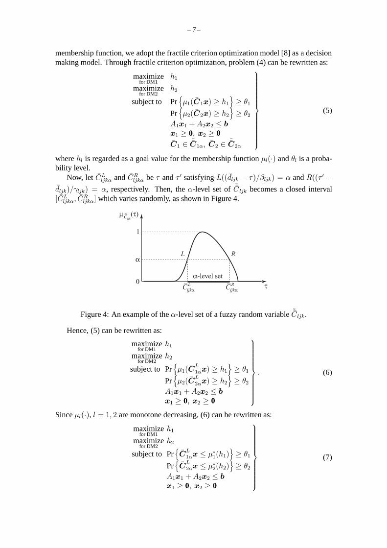
Now, let CLljkα andCR

ljkα beτ andτ ′ satisfyingL((dljk − τ )/βljk) = α andR((τ ′ −dljk)/γljk) = α, respectively. Then, theα-level set of ˜C ljk becomes a closed interval[CL

ljkα, CRljkα] which varies randomly, as shown in Figure 4.

Figure 4: An example of theα-level set of a fuzzy random variableCljk.

Hence, (5) can be rewritten as:

maximizefor DM1

h1

maximizefor DM2

h2

subject to Prµ1(C

L1αx) ≥ h1

≥ θ1

Prµ2(C

L2αx) ≥ h2

≥ θ2

A1x1 +A2x2 ≤ bx1 ≥ 0, x2 ≥ 0

. (6)

Sinceµl(·), l = 1, 2 are monotone decreasing, (6) can be rewritten as:

maximizefor DM1

h1

maximizefor DM2

h2

subject to PrCL1αx ≤ µ∗1(h1)

≥ θ1

PrCL2αx ≤ µ∗2(h2)

≥ θ2

A1x1 +A2x2 ≤ bx1 ≥ 0, x2 ≥ 0

(7)

– 8 –

whereµ∗l (·) is a pseudo-inverse function ofµl(·) defined byµ∗l (hl) = supy | µl(y) ≥hl.

In view of α = L((dljk − CLljkα)/βljk) in (7), it holds that

CLljkα = dljk − L∗(α) · βljk

whereL∗(·) is a pseudo-inverse function ofL(·) defined byL∗(α) = supτ | L(τ ) ≥ α.From this result, the left side of the first and second constraint in (7) can be expressed as:

PrCLlαx ≤ µ∗l (hl)

= Pr

(dl − L∗(α) · βl)x ≤ µ∗l (hl)

.

Recalling the assumption thatdl is an(n1+n2) dimensional Gaussian random variablerow vector with mean vectorM l and positive-definite covariance matrixVl, it holds that

Pr

(dl − L∗(α) · βl)x ≤ µ∗l (hl)

= Prdlx ≤ L∗(α) · βlx+ µ∗l (hl)

= Pr

dlx−M lx√

xTVlx≤ L∗(α) · βlx−M lx+ µ∗l (hl)√

xTVlx

= Φ

((L∗(α) · βl −M l)x+ µ∗l (hl)√

xTVlx

)

whereΦ(·) is the probability distribution of a standard Gaussian distribution with mean 0and variance 1. From the above results it can be shown that

Φ

((L∗(α) · βl −M l)x+ µ∗l (hl)√

xTVlx

)≥ θl

⇔ (L∗(α) · βl −M l)x+ µ∗l (hl)√xTVlx

≥ Φ−1l (θl)

⇔ µ∗l (hl) ≥ (M l − L∗(α) · βl)x+ Φ−1l (θl)

√xTVlx

⇔ hl ≤ µl

((M l − L∗(α) · βl)x+ Φ−1

l (θl)√xTVlx

)whereΦ−1

l (·) is the inverse function ofΦl(·).In this way, (7) can be transformed as:

maximizefor DM1

h1

maximizefor DM2

h2

subject to µ1

(ZF

1α(x))≥ h1

µ2

(ZF

2α(x))≥ h2

A1x1 +A2x2 ≤ bx1 ≥ 0, x2 ≥ 0

(8)

equivalently,maximize

for DM1µ1

(ZF

1α(x))

maximizefor DM2

µ2

(ZF

2α(x))

subject toA1x1 +A2x2 ≤ bx1 ≥ 0, x2 ≥ 0

(9)

– 9 –

whereZFlα(x) = (M l − L∗(α) · βl)x+ Φ−1

l (θl)√xTVlx. (10)

In this equation, recalling that the covariance matrix is assumed to be positive-definite, Itis evident that

√xTVlx is convex andZF

lα(x) is also convex ifΦ−1l (θl) > 0, i.e.,θl > 0.5,

l = 1, 2.

5 Interactive fuzzy programming

Observing the transformed problem (9) is a deterministic two-level programming prob-lem, we can now construct the interactive algorithm to derive a satisfactory solution forthe decision maker at the upper level in consideration of the cooperative relationshipsbetween DM1 and DM2,

Interactive fuzzy programming

Step 1 In order to calculate the individual minimum and maximum of Ezl(x1,x2) =M lx, solve the following problems:

minimize M lxsubject toA1x1 +A2x2 ≤ b

x1 ≥ 0, x2 ≥ 0

, l = 1, 2, (11)

maximize M lxsubject toA1x1 +A2x2 ≤ b

x1 ≥ 0, x2 ≥ 0

, l = 1, 2. (12)

Let zEl,min andzEl,max be the the minimal objective function value to (11) and themaximal objective function value to (12), respectively. Observing that (11) and(12) are linear programming problems, they can be easily solved by some linearprogramming technique like the simplex method.

Step 2 Ask the decision makers to determine the membership functionsµl(·), l = 1, 2 byconsidering the obtained values ofzEl,min andzEl,max, l = 1, 2.

Step 3 Ask DM1 to specify the initial value of the degree of realizationα ∈ (0, 1) andthat of the probability levelθl(> 0.5), l = 1, 2.

Step 4 For the specified values ofα andθl, l = 1, 2, the following problem is solved forobtaining a solution which maximizes the smaller degree of satisfaction betweenthose of the two decision makers:

maximize minµ1

(ZF

1α(x)), µ2

(ZF

2α(x))

subject toA1x1 +A2x2 ≤ bx1 ≥ 0, x2 ≥ 0

(13)

equivalently,maximize v

subject to µ1

(ZF

1α(x))≥ v

µ2

(ZF

2α(x))≥ v

A1x1 +A2x2 ≤ bx1 ≥ 0, x2 ≥ 0

. (14)

– 10 –

In view of (10), this problem is rewritten as:

maximize vsubject to µ1

((M 1 − L∗(α) · β1)x+ Φ−1

1 (θ1)√xTV1x

)≥ v

µ2

((M 2 − L∗(α) · β2)x+ Φ−1

2 (θ2)√xTV2x

)≥ v

A1x1 +A2x2 ≤ bx1 ≥ 0, x2 ≥ 0

(15)

equivalently,

maximize v

subject to (M1 − L∗(α) · β1)x+ Φ−11 (θ1)

√xTV1x ≤ µ∗1(v)

(M2 − L∗(α) · β2)x+ Φ−12 (θ2)

√xTV2x ≤ µ∗2(v)

A1x1 +A2x2 ≤ bx1 ≥ 0, x2 ≥ 0

. (16)

Obtaining the optimal value ofv to this problem is equivalent to finding the max-imum of v so that the set of feasible solutions to (16) is not empty. Although thisproblem is a nonlinear programming problem, we can easily find the maximum ofv by the following algorithm on the basis of the bisection method and some con-vex programming technique like the sequential quadratic programming since theconstraints of (16) are convex ifv is fixed.

The combined use of the bisection method and the sequential quadraticprogramming

4-1 Set l := 0 and v := 0. Test whether the set of feasible solutions to (16)for v = 0 is empty or not using the sequential quadratic programming. If itis empty, the decision makers must reassess membership functions,α or θl.Otherwise, letvfeasible:= v and go to 4-2

4-2 Setv := 1. Test whether the set of feasible solutions to (16) forv = 1 is emptyor not using the sequential quadratic programming . If it is not empty,v = 1is the optimal valuev∗ to (16) and the algorithm is terminated. Otherwise, themaximum ofv so that the set of feasible solutions to (16) is not empty existsbetween0 and1. Let vinfeasible:= v and go to 4-3.

4-3 Setv := (vfeasible+ vinfeasible)/2, l := l + 1 and go to 4-4.

4-4 Test whether the set of feasible solutions to (16) forv determined in 4-3 isempty or not using the sequential quadratic programming. If it is not emptyand(1/2)l ≤ ε, the current value ofv is regarded as the optimal valuev∗ to(16) and the algorithm is terminated. If it is not empty and(1/2)l > ε, letvfeasible:= v and return to 4-3. On the other hand, if it is empty, letvinfeasible:=v and return to 4-3.

Then, for the obtained optimal valuev∗, we can determine the corresponding opti-mal valuex∗ by solving the following convex programming problem:

minimize (M1 − L∗(α) · β1)x+ Φ−11 (θ1)

√xTV1x

subject to (M2 − L∗(α) · β2)x+ Φ−12 (θ2)

√xTV2x ≤ µ∗2(v∗)

A1x1 +A2x2 ≤ bx1 ≥ 0, x2 ≥ 0

. (17)

– 11 –

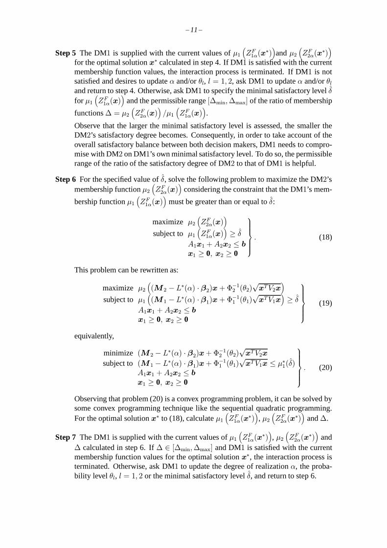
Step 5 The DM1 is supplied with the current values ofµ1

(ZF

1α(x∗))andµ2

(ZF

2α(x∗))

for the optimal solutionx∗ calculated in step 4. If DM1 is satisfied with the currentmembership function values, the interaction process is terminated. If DM1 is notsatisfied and desires to updateα and/orθl, l = 1, 2, ask DM1 to updateα and/orθland return to step 4. Otherwise, ask DM1 to specify the minimal satisfactory levelδfor µ1

(ZF

1α(x))

and the permissible range[∆min,∆max] of the ratio of membership

functions∆ = µ2

(ZF

2α(x))/µ1

(ZF

1α(x)).

Observe that the larger the minimal satisfactory level is assessed, the smaller theDM2’s satisfactory degree becomes. Consequently, in order to take account of theoverall satisfactory balance between both decision makers, DM1 needs to compro-mise with DM2 on DM1’s own minimal satisfactory level. To do so, the permissiblerange of the ratio of the satisfactory degree of DM2 to that of DM1 is helpful.

Step 6 For the specified value ofδ, solve the following problem to maximize the DM2’smembership functionµ2

(ZF

2α(x))

considering the constraint that the DM1’s mem-

bership functionµ1

(ZF

1α(x))

must be greater than or equal toδ:

maximize µ2

(ZF

2α(x))

subject to µ1

(ZF

1α(x))≥ δ

A1x1 +A2x2 ≤ bx1 ≥ 0, x2 ≥ 0

. (18)

This problem can be rewritten as:

maximize µ2

((M 2 − L∗(α) · β2)x+ Φ−1

2 (θ2)√xTV2x

)subject to µ1

((M 1 − L∗(α) · β1)x+ Φ−1

1 (θ1)√xTV1x

)≥ δ

A1x1 +A2x2 ≤ bx1 ≥ 0, x2 ≥ 0

(19)

equivalently,

minimize (M 2 − L∗(α) · β2)x+ Φ−12 (θ2)

√xTV2x

subject to (M 1 − L∗(α) · β1)x+ Φ−11 (θ1)

√xTV1x ≤ µ∗1(δ)

A1x1 +A2x2 ≤ bx1 ≥ 0, x2 ≥ 0

. (20)

Observing that problem (20) is a convex programming problem, it can be solved bysome convex programming technique like the sequential quadratic programming.For the optimal solutionx∗ to (18), calculateµ1

(ZF

1α(x∗)), µ2

(ZF

2α(x∗))

and∆.

Step 7 The DM1 is supplied with the current values ofµ1

(ZF

1α(x∗)), µ2

(ZF

2α(x∗))

and∆ calculated in step 6. If∆ ∈ [∆min,∆max] and DM1 is satisfied with the currentmembership function values for the optimal solutionx∗, the interaction process isterminated. Otherwise, ask DM1 to update the degree of realizationα, the proba-bility level θl, l = 1, 2 or the minimal satisfactory levelδ, and return to step 6.

– 12 –

In the proposed algorithm,∆min and ∆max are usually set to be less than1 sinceµ1

(ZF

1α(x∗))

should be greater thanµ2

(ZF

2α(x∗))

because of the priority of DM1. In step

6, if ∆ < ∆min, i.e.,µ1

(ZF

1α(x∗))

is much greater thanµ2

(ZF

2α(x∗)), DM1 will decrease

δ to improveµ2

(ZF

2α(x∗))

and increase∆. Otherwise, if∆max < ∆, i.e.,µ1

(ZF

1α(x∗))

is

slightly greater or less thanµ2

(ZF

2α(x∗)), DM1 will increaseδ to improveµ1

(ZF

1α(x∗))

and decrease∆. On the other hand, if DM1 decreases (increases)α and/orθl, l = 1, 2,bothµ1

(ZF

1α(x∗))

andµ2

(ZF

2α(x∗))

would increase (decrease). With this observation,

it can be expected that desirable values ofµ1

(ZF

1α(x∗)), µ2

(ZF

2α(x∗))

and∆ will be

obtained through a series of update procedures ofδ, α and/orθl, l = 1, 2 with DM1.

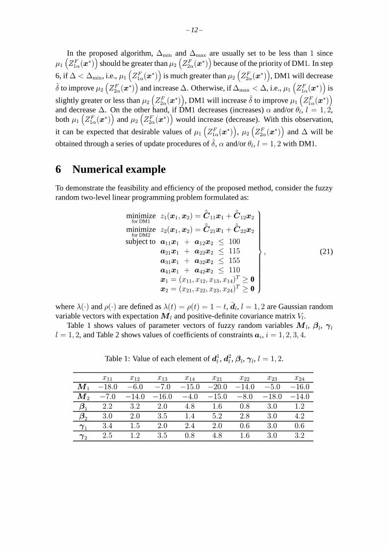
6 Numerical example

To demonstrate the feasibility and efficiency of the proposed method, consider the fuzzyrandom two-level linear programming problem formulated as:

minimizefor DM1

z1(x1,x2) = ˜C11x1 + ˜C12x2

minimizefor DM2

z2(x1,x2) = ˜C21x1 + ˜C22x2

subject to a11x1 + a12x2 ≤ 100a21x1 + a22x2 ≤ 115a31x1 + a32x2 ≤ 155a41x1 + a42x2 ≤ 110x1 = (x11, x12, x13, x14)T ≥ 0x2 = (x21, x22, x23, x24)T ≥ 0

, (21)

whereλ(·) andρ(·) are defined asλ(t) = ρ(t) = 1− t, dl, l = 1, 2 are Gaussian randomvariable vectors with expectationM l and positive-definite covariance matrixVl.

Table 1 shows values of parameter vectors of fuzzy random variablesM l, βl, γ ll = 1, 2, and Table 2 shows values of coefficients of constraintsai, i = 1, 2, 3, 4.

Table 1: Value of each element ofd1l , d

2l , βl, γl, l = 1, 2.

x11 x12 x13 x14 x21 x22 x23 x24

M1 −18.0 −6.0 −7.0 −15.0 −20.0 −14.0 −5.0 −16.0M2 −7.0 −14.0 −16.0 −4.0 −15.0 −8.0 −18.0 −14.0β1 2.2 3.2 2.0 4.8 1.6 0.8 3.0 1.2β2 3.0 2.0 3.5 1.4 5.2 2.8 3.0 4.2γ1 3.4 1.5 2.0 2.4 2.0 0.6 3.0 0.6γ2 2.5 1.2 3.5 0.8 4.8 1.6 3.0 3.2

– 13 –

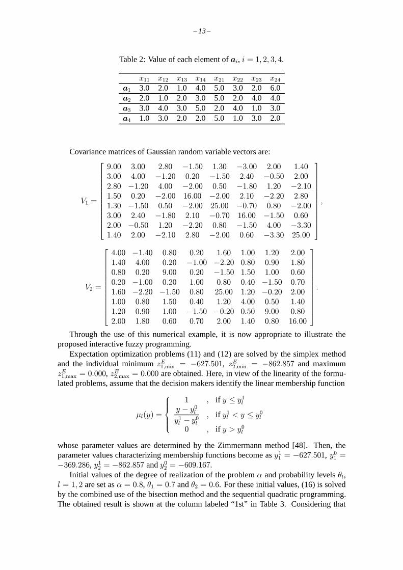
Table 2: Value of each element ofai, i = 1, 2, 3, 4.

x11 x12 x13 x14 x21 x22 x23 x24

a1 3.0 2.0 1.0 4.0 5.0 3.0 2.0 6.0a2 2.0 1.0 2.0 3.0 5.0 2.0 4.0 4.0a3 3.0 4.0 3.0 5.0 2.0 4.0 1.0 3.0a4 1.0 3.0 2.0 2.0 5.0 1.0 3.0 2.0

Covariance matrices of Gaussian random variable vectors are:

V1 =

9.00 3.00 2.80 −1.50 1.30 −3.00 2.00 1.403.00 4.00 −1.20 0.20 −1.50 2.40 −0.50 2.002.80 −1.20 4.00 −2.00 0.50 −1.80 1.20 −2.101.50 0.20 −2.00 16.00 −2.00 2.10 −2.20 2.801.30 −1.50 0.50 −2.00 25.00 −0.70 0.80 −2.003.00 2.40 −1.80 2.10 −0.70 16.00 −1.50 0.602.00 −0.50 1.20 −2.20 0.80 −1.50 4.00 −3.301.40 2.00 −2.10 2.80 −2.00 0.60 −3.30 25.00

,

V2 =

4.00 −1.40 0.80 0.20 1.60 1.00 1.20 2.001.40 4.00 0.20 −1.00 −2.20 0.80 0.90 1.800.80 0.20 9.00 0.20 −1.50 1.50 1.00 0.600.20 −1.00 0.20 1.00 0.80 0.40 −1.50 0.701.60 −2.20 −1.50 0.80 25.00 1.20 −0.20 2.001.00 0.80 1.50 0.40 1.20 4.00 0.50 1.401.20 0.90 1.00 −1.50 −0.20 0.50 9.00 0.802.00 1.80 0.60 0.70 2.00 1.40 0.80 16.00

.

Through the use of this numerical example, it is now appropriate to illustrate theproposed interactive fuzzy programming.

Expectation optimization problems (11) and (12) are solved by the simplex methodand the individual minimumzE1,min = −627.501, zE2,min = −862.857 and maximumzE1,max = 0.000, zE2,max = 0.000 are obtained. Here, in view of the linearity of the formu-lated problems, assume that the decision makers identify the linear membership function

µl(y) =

1 , if y ≤ y1

l

y − y0l

y1l − y0

l

, if y1l < y ≤ y0

l

0 , if y > y0l

whose parameter values are determined by the Zimmermann method [48]. Then, theparameter values characterizing membership functions become asy1

1 = −627.501, y01 =

−369.286, y12 = −862.857 andy0

2 = −609.167.Initial values of the degree of realization of the problemα and probability levelsθl,

l = 1, 2 are set asα = 0.8, θ1 = 0.7 andθ2 = 0.6. For these initial values, (16) is solvedby the combined use of the bisection method and the sequential quadratic programming.The obtained result is shown at the column labeled “1st” in Table 3. Considering that

– 14 –

both of the membership function values are a little low, DM1 updatesα from 0.8 to 0.7.For the updated value ofα, the corresponding problem (16) is solved, and the obtainedresult is shown at the column labeled “2nd” in Table 3. DM1 is not satisfied with thissolution, but he does not desire to updateα, θ1 or θ2 since the membership functionvalues are improved. Thus, DM1 determines the minimal satisfactory levelδ = 0.70 toimproveµ1 (the satisfactory degree of DM1) at the expense ofµ2 (the satisfactory degreeof DM2). Furthermore, DM1 specifies the upper bound∆max = 0.85 and the lower bound∆min = 0.75 for the ratio of membership functions∆ = µ2/µ1. For the updated value ofδ = 0.70 , (20) is solved by the sequential quadratic programming. The obtained result isshown at the column labeled “3rd” in Table 3.

For the current values ofµ1, µ2 and∆, DM1 considers thatµ1 is improved butµ2

is too bad, and∆ is less than∆min. Hence, DM1 is not satisfied with this solution andupdates the minimal satisfactory levelδ from 0.70 to 0.60. For the updated value ofδ,(20) is solved and the obtained result is shown at the column labeled “4th” in Table 3.Sinceµ2 is improved but∆ is greater than∆max, DM1 is not satisfied with this solutionand updates the minimal satisfactory levelδ from 0.60 to 0.65. For the updated value ofδ, (20) is solved and the obtained result is shown at the column labeled “5th” in Table3. In this example, since∆ exists in the interval[∆min,∆max] and DM1 is satisfied withthe overall satisfactory balance betweenµ1 andµ2, at the 5th iteration, the interactivealgorithm is terminated.

Table 3: Interaction process.

Interaction 1st 2nd 3rd 4th 5thα 0.800 0.700 0.700 0.700 0.700θ1 0.700 0.700 0.700 0.700 0.700θ2 0.600 0.600 0.600 0.600 0.600δ — — 0.700 0.600 0.650

µ1

(ZF

1α(x))

0.525 0.579 0.700 0.600 0.650

µ2

(ZF

2α(x))

0.525 0.579 0.459 0.579 0.531∆ 1.000 1.000 0.698 0.965 0.816

In the proposed interactive fuzzy programming, through a series of update proceduresof the minimal satisfactory levelδ, the degree of realizationα and the probability levelθl,l = 1, 2, it can be possible to obtain a satisfactory solution where the satisfactory degreeof DM1 is guaranteed to be greater than or equal to the minimal satisfactory levelδ andis well balanced with that of DM2.

7 Conclusions

In this paper, assuming cooperative behavior of the decision makers, interactive decisionmaking methods in hierarchical organizations under fuzzy random environments wereconsidered. For the formulated fuzzy random two-level linear programming problems,

– 15 –

α-level sets of fuzzy random variables were introduced and anα-stochastic two-level lin-ear programming problem was defined for guaranteeing the degree of realization of theproblem. Considering the vague natures of decision makers’ judgments, fuzzy goals wereintroduced and theα-stochastic two-level linear programming problem was transformedinto the problem to maximize the satisfaction degree for each fuzzy goal. Through thefractile criterion optimization model, the transformed stochastic two-level programmingproblem was reduced to a deterministic one. Interactive fuzzy programming to obtain asatisfactory solution for the decision maker at the upper level in consideration of the co-operative relation between decision makers was presented. It should be emphasized herethat all problems to be solved in the proposed interactive fuzzy programming can be eas-ily solved by the simplex method, the sequential quadratic programming or the combineduse of the bisection method and the sequential quadratic programming. An illustrativenumerical example demonstrated the feasibility and efficiency of the proposed method.Extensions to other stochastic programming models will be considered elsewhere. Alsoextensions to fuzzy random two-level linear programming problems with two decisionmakers under noncooperative environments will be required in the near future.

References

[1] M.A. Abo-Sinna, I.A. Baky, Interactive balance space approach for solving multi-level multi-objective programming problems, Information Sciences 177 (2007)3397–3410.

[2] E.E. Ammar, On solutions of fuzzy random multiobjective quadratic programmingwith applications in portfolio problem, Information Sciences 178 (2008) 468–484.

[3] W.F. Bialas, M.H. Karwan, Two-level linear programming, Management Science 30(1984) 1004–1020.

[4] J.R. Birge, F. Louveaux, Introduction to Stochastic Programming, Springer, London,1997.

[5] A. Charnes, W.W. Cooper, Chance constrained programming, Management Science6 (1959) 73–79.

[6] A. Charnes, W.W. Cooper, Deterministic equivalents for optimizing and satisficingunder chance constraints, Operations Research 11 (1963) 18–39.

[7] M.A. Gil, M. Lopez-Diaz, D.A. Ralescu, Overview on the development of fuzzyrandom variables, Fuzzy Sets and Systems 157 (2006) 2546–2557.

[8] S. Kataoka, A stochastic programming model, Econometorica 31 (1963) 181–196.

[9] H. Katagiri, H. Ishii and M. Sakawa, On fuzzy random linear knapsack problems,Central European Journal of Operations Research 12 (2004) 59–70.

[10] H. Katagiri, E.B. Mermri, M. Sakawa, K. Kato, I. Nishizaki, A possibilistic andstochastic programming approach to fuzzy random MST problems, IEICE Transac-tion on Information and Systems E88-D (2005) 1912–1919.

– 16 –

[11] H. Katagiri, M. Sakawa, H. Ishii, A study on fuzzy random portfolio selection prob-lems using possibility and necessity measures, Scientiae Mathematicae Japonicae61 (2005) 361–369.

[12] H. Katagiri, M. Sakawa, K. Kato, I. Nishizaki, A fuzzy random multiobjective 0-1 programming based on the expectation optimization model using possibility andnecessity measures, Mathematical and Computer Modelling 40 (2004) 411–421.

[13] H. Katagiri, M. Sakawa, K. Kato, I. Nishizaki, Interactive multiobjective fuzzy ran-dom linear programming: maximization of possibility and probability, EuropeanJournal of Operational Research 188 (2008) 530–539.

[14] H. Katagiri, M. Sakawa, I. Nishizaki, Interactive decision making using possibilityand necessity measures for a fuzzy random multiobjective 0-1 programming prob-lem, Cybernetics and Systems 37 (2006) 59–74.

[15] R. Kruse, K.D. Meyer, Statistics with Vague Data, D. Riedel Publishing Company,1987.

[16] H. Kwakernaak, Fuzzy random variables - I. definitions and theorems, InformationSciences 15 (1978) 1–29.

[17] Y.J. Lai, Hierarchical optimization: a satisfactory solution, Fuzzy Sets and Systems77 (1996) 321–325.

[18] E.S. Lee, Fuzzy multiple level programming, Applied Mathematics and Computa-tion 120 (2001) 79–90.

[19] B. Liu, Fuzzy random chance-constrained programming, IEEE Transaction onFuzzy Systems 9 (2001) 713–720.

[20] B. Liu, Fuzzy random dependent-chance programming, IEEE Transaction on FuzzySystems 9 (2001) 721–726.

[21] Y.-K. Liu, B. Liu, Fuzzy Random Variables: A Scalar Expected Value Operator,Fuzzy Optimization and Decision Making 2 (2003) 143–160.

[22] M.K. Luhandjula, Fuzziness and randomness in an optimization framework, FuzzySets and Systems 77 (1996) 291–297.

[23] M.K. Luhandjula, Fuzzy stochastic linear programming: survey and future researchdirections, European Journal of Operational Research 174 (2006) 1353–1367.

[24] M.K. Luhandjula, M.M. Gupta, On fuzzy stochastic optimization, Fuzzy Sets andSystems 81 (1996) 47–55.

[25] I. Nishizaki, M. Sakawa, Computational methods through genetic algorithms for ob-taining Stackelberg solutions to two-level mixed zero-one programming problems,Cybernetics and Systems: An International Journal 31 (2000) 203–221.

[26] S. Pramanik, T.K. Roy, Fuzzy goal programming approach to multilevel program-ming problems, European Journal of Operational Research 176 (2007) 1151–1166.

– 17 –

[27] M.L. Puri, D.A. Ralescu, Fuzzy random variables, Journal of Mathematical Analysisand Applications 114 (1986) 409–422.

[28] Z. Qaio, Y. Zhang, G.-Y. Wang, On fuzzy random linear programming, Fuzzy Setsand Systems 65 (1994) 31–49.

[29] E. Roghanian, S.J. Sadjadi, M.B. Aryanezhad, A probabilistic bi-level linear multi-objective programming problem to supply chain planning, Applied Mathematics andComputation 188 (2007) 786–800.

[30] H. Rommelfanger, A general concept for solving linear multicriteria programmingproblems with crisp, fuzzy or stochastic values, Fuzzy Sets and Systems 156 (2007)1892–1904.

[31] M. Sakawa, Fuzzy Sets and Interactive Multiobjective Optimization, Plenum Press,New York, 1993.

[32] M. Sakawa, I. Nishizaki, Interactive fuzzy programming for decentralized two-levellinear programming problems, Fuzzy Sets and Systems 125 (2002) 301–315.

[33] M. Sakawa, I. Nishizaki, Interactive fuzzy programming for two-level nonconvexprogramming problems with fuzzy parameters through genetic algorithms, FuzzySets and Systems 127 (2002) 185–197.

[34] M. Sakawa, I. Nishizaki, Cooperative and Noncooperative Multi-Level Program-ming, Springer, Norwell (in press).

[35] M. Sakawa, I. Nishizaki, Y. Uemura, Interactive fuzzy programming for multi-levellinear programming problems, Computers & Mathematics with Applications 36(1998) 71–86.

[36] M. Sakawa, I. Nishizaki, Y. Uemura, Interactive fuzzy programming for two-levellinear fractional programming problems with fuzzy parameters, Fuzzy Sets and Sys-tems 115 (2000) 93–103.

[37] M. Sakawa, I. Nishizaki, Y. Uemura, Interactive fuzzy programming for two-levellinear and linear fractional production and assignment problems: a case study, Eu-ropean Journal of Operational Research 135 (2001) 142–157.

[38] M. Sakawa, I. Nishizaki, Y. Uemura, A decentralized two-level transportation prob-lem in a housing material manufacturer –Interactive fuzzy programming approach–,European Journal of Operational Research 141 (2002) 167–185.

[39] H.S. Shih, Y.J. Lai, E.S. Lee, Fuzzy approach for multi-level programming prob-lems, Computers and Operations Research 23 (1996) 73–91.

[40] K. Shimizu, Y. Ishizuka, J.F. Bard, Nondifferentiable and Two-Level MathematicalProgramming, Kluwer Academic Publishers, Boston, 1997.

[41] M. Simaan, J.B. Cruz Jr., On the Stackelberg strategy in nonzero-sum games, Journalof Optimization Theory and Applications 11 (1973) 533–555.

– 18 –

[42] S. Sinha, Fuzzy programming approach to multi-level programming problems,Fuzzy Sets and Systems 136 (2003) 189–202.

[43] I.M. Stancu-Minasian, Stochastic Programming with Multiple Objective Functions,D. Reidel Publishing Company, Dordrecht, 1984.

[44] I.M. Stancu-Minasian, Overview of different approaches for solving stochas-tic programming problems with multiple objective functions, R. Slowinski andJ. Teghem (eds.):Stochastic Versus Fuzzy Approaches to Multiobjective Math-ematical Programming under Uncertainty, Kluwer Academic Publishers, Dor-drecht/Boston/London, pp. 71–101, 1990.

[45] G.-Y. Wang, Z. Qiao, Linear programming with fuzzy random variable coefficients,Fuzzy Sets and Systems 57 (1993) 295–311.

[46] R.J.B. Wets, Challenges in stochastic programming, Mathematical Programming 75(1996) 115–135.

[47] J. Xu, Y. Liu, Multi-objective decision making model under fuzzy random environ-ment and its application to inventory problems, Information Sciences 178 (2008)2899–2914.

[48] H.-J. Zimmermann, Fuzzy programming and linear programming with several ob-jective functions, Fuzzy Sets and Systems 1 (1978) 45–55.