international union for the protection … · international union for the protection of new...
TRANSCRIPT

ETGP/8/1 Draft 1ORIGINAL: EnglishDATE: June 2, 2005
INTERNATIONAL UNION FOR THE PROTECTION OF NEW VARIETIES OF PLANTSGENEVA
DRAFT
Associated Document to the
General Introduction to the Examinationof Distinctness, Uniformity and Stability and the
Development of Harmonized Descriptions of New Varieties of Plants (document TG/1/3)
DOCUMENT TGP/8
“USE OF STATISTICAL PROCEDURES IN
DISTINCTNESS, UNIFORMITY AND STABILITY TESTING”
Document prepared by the Office of the Union
to be considered by the
Technical Working Party for Vegetables (TWV), at its thirty-ninth session to be held inNitra, Slovakia, from June 6 to 10, 2005
Technical Working Party on Automation and Computer Programs (TWC),at its twenty-third session to be held in Ottawa, from June 13 to 16, 2005
Technical Working Party for Fruit Crops (TWF), at its thirty-sixth session to be held inKofu, Japan, from September 5 to 9, 2005
Technical Working Party for Ornamental Plants and Forest Trees (TWO),at its thirty-eighth session to be held in Seoul, from September 12 to 16, 2005
Technical Working Party for Agricultural Crops (TWA), at its thirty-fourth session to be heldin Christchurch, New Zealand, from October 31 to November 4, 2005

TGP/8/1 Draft 1page 2
TABLE OF CONTENTSSECTION I: INTRODUCTION ............................................................................................................................4
1. Aim 42. Observable characteristics and variation ..........................................................................................43. Why use statistical procedures?........................................................................................................44. Why replicate?..................................................................................................................................45. Why randomize?...............................................................................................................................46. Further benefits of randomization.....................................................................................................57. Direct comparison and randomization..............................................................................................58. Variety is the treatment.....................................................................................................................59. The crop makes the difference in testing ..........................................................................................510. The expert and statistical computation .............................................................................................611. UPOV, statistical computation and harmonization...........................................................................612. Recapitulation with reference to subsequent chapters: .....................................................................6
SECTION 2: EXPERIMENTAL DESIGN PRACTICES .....................................................................................82.1 Introduction ......................................................................................................................................82.2 Trials, experimental units and test of hypotheses .............................................................................92.3 From a complete randomized design to a randomized complete block design...............................112.4 Randomized incomplete block designs...........................................................................................132.5 Pairwise comparisons of some varieties .........................................................................................142.6 Trial elements .................................................................................................................................152.7 Sample size....................................................................................................................................172.8 Analyses over years or cycles.........................................................................................................17
SECTION 3: TYPES OF CHARACTERISTICS AND THEIR SCALE LEVELS.............................................183.1 Introduction ....................................................................................................................................183.2 Different levels to look at a characteristic ......................................................................................183.3 Types of expression of characteristics ............................................................................................193.4 Types of scales of data....................................................................................................................203.5 Scale levels for variety description.................................................................................................243.6 Relation between types of expression of characteristics and scale levels of data...........................243.7 Relation between method of observation of characteristics, scale levels of data and recommendedstatistical procedures..................................................................................................................................26
SECTION 4: VALIDATION OF DATA AND ASSUMPTIONS.......................................................................314.1 Introduction ....................................................................................................................................314.2 Check on data quality (before doing analyses) ...............................................................................314.3 Assumptions ...................................................................................................................................334.4 Validation36
SECTION 5: STATISTICAL METHODS FOR DUS EXAMINATION ...........................................................415.1 Analysis of variance .......................................................................................................................41
SECTION 6: EXAMINING DUS IN BULK SAMPLES....................................................................................536.1 Introduction and abstract ................................................................................................................536.2 Distinctness.....................................................................................................................................536.3 Uniformity ......................................................................................................................................55
SECTION 7: THE GAIA METHODOLOGY .....................................................................................................577.1. Weighting of characteristics ........................................................................................................... 577.2. Determining “Distinctness Plus” ................................................................................................... 587.3. Computing GAIA phenotypic distance............................................................................................ 597.4. The GAIA software ......................................................................................................................... 597.5. Using the GAIA methodology ......................................................................................................... 627.6. Example with qualitative, electrophoretic and quantitative characteristics (Zea mays data)........ 637.7 GAIA screen copy. .......................................................................................................................... 697.8 Final remark................................................................................................................................... 70
REFERENCES......................................................................................................................................................71APPENDICES ......................................................................................................................................................72
APPENDIX A1 ............................................................................................................................................ 72Example of two-way ANOVA (same type as Example A) ........................................................... 72Example of two-way ANOVA (same type as Example B) ........................................................... 73
APPENDIX A2 ............................................................................................................................................ 75Example of one-way ANOVA (same type as Example C) ........................................................... 75Example of one-way ANOVA (same type as Example D) ........................................................... 76

TGP/8/1 Draft 1page 3
APPENDIX A3 ............................................................................................................................................ 78Example of a paired t-test (same type as Example E) ................................................................... 78The paired t-test analysis using a one-sample t-test of differences ............................................... 78The paired t-test analysis using two-way ANOVA....................................................................... 79
APPENDIX A4 ............................................................................................................................................ 815.2 The Combined Over-Years Distinctness Criterion (COYD) ........................................................... 81
5.2.1 Summary .......................................................................................................................... 815.2.2 Introduction...................................................................................................................... 815.2.3 The COYD Method.......................................................................................................... 82
5.3 UPOV Recommendations on COYD............................................................................................... 835.4 Adapting COYD to special circumstances...................................................................................... 835.5 Small numbers of varieties in trials: Long-Term COYD ................................................................ 835.6 Marked year-to-year changes in an individual variety’s characteristic......................................... 845.7 Implementing COYD....................................................................................................................... 84

TGP/8/1 Draft 1page 4
SECTION I: INTRODUCTION
1. Aim
This introduction will briefly cover the key-elements on statistics as used in the examinationof DUS. It is meant to encourage the reading of subsequent chapters that elaborate on theseelements. To arrive at an objective decision when testing and comparing different items, it isimportant to be aware of the basic statistical notions and practices.
2. Observable characteristics and variation
The requirements are formulated and recorded in (‘absolute’) observable characteristics thatare used to assess distinctness (D) between varieties, uniformity (U) within a variety andstability (S) over years for varieties. It is thus generally referred to as DUS-testing. Thenature of the object of interest, a plant variety, makes it susceptible to all kinds of externalinfluences, e.g. growing conditions like latitude, climate, soil, irrigation etc. which rendervariation in the expression of the characteristics observed between plants. But there are alsoaspects that may lead to variation (or the lack of it) in the observed characteristic of a givenvariety because of the type of variety e.g. the way it is propagated (e.g. cross-pollinated vs.vegetative propagation, seed/bulb/tuber size etc). We must also bear in mind that measuring acharacteristic leads to yet another source of variation; the measurement error. All theseelements of variation in our observations are to be taken into account in a model agreed byUPOV for proper analysis. These topics are pursued later on.
3. Why use statistical procedures?
Each observation contains a mixture of all these sources of variation and it is good practice tohave some basic notion of their magnitudes (if possible). At the end of the run this willdetermine the reliability of the measurements and that is what statistics is all about and whywe need statistical procedures for a judgement.
4. Why replicate?
The first key element of experimentation in a statistical context is replication. This can eitherbe determining the number of off-types in e.g. sixty plants in only one experiment or on 20separate plants per plot in 3-replicated blocks for 3 consecutive years. In all cases, thereplication gives us a handle on hypothesis testing: is the candidate variety different from therest by some observed characteristic that exceeds the noise that is basic to the wholeexperiment? This noise, present in all observations (=experimental error), acts as a yard-stickto judge differences in the experiment (i.e. distinctness). When the characteristic is lessconsistent, the difference for a decision needs to be accordingly greater. Moreover theobservations on the replications can be used as a uniformity measure.
5. Why randomize?
The second key element is randomization for each experiment. This ensures that allunknown sources of variation have an equal chance of acting upon the varieties tested, and noaccidental systematic effect is recorded due to e.g. germination, planting, growing, harvesting,recording etc. In those cases where specific ordering is required to observe a characteristic(e.g. comparison of colour or architecture) one should be aware that this is only (reluctantly)admissible in one replication, and one should be careful with conclusions on other

TGP/8/1 Draft 1page 5
measurements. This brings our focus to a case where some grouping is required becauseotherwise competition would influence the observation, e.g. early varieties would hamper thedevelopment of late ones. In those cases it is crucial to randomize within and between groupsof the experiment, as experiments are carried out over the years and groups should then bearranged differently to avoid systematic effects.
6. Further benefits of randomization
Proper randomization makes our conclusions valid/predictive for all similar experiments, andnot only for one specific experiment of which the results might have been caused by someunknown systematic effects, e.g. ordering of varieties, some fertility trend/spot in the soil orrecording time during the day. Randomization will also prevent us from working with anunrealistic small experimental error that cannot be reproduced, e.g. by close comparison ofspecific varieties or when all varieties are lined up in the field based on one characteristic.Randomization will also enhance objective recording of the characteristic.
7. Direct comparison and randomization
It is nevertheless common practice to plant varieties which show little difference betweenthem side-by-side or in the same area. This allows better evaluation by the experts during thedifferent visits and observations through direct comparison in the field for difficult cases. Asalready stated this does not invalidate the statistical reliability too much if it is confined to onereplication in a blocked trial, or if at least different orderings are used in different blocks andin different trials. One should be aware that the yardstick used for discrimination on the othercharacteristics is not as reliable in this case, as the special arrangement can only be based onone or two characteristics(s). Close scrutiny in one characteristic may introduce systematic orinteraction effects (bias) for others, so more care is needed in the interpretation.
8. Variety is the treatment
The third key element is the experimental (main) treatment, for the purposes of DUSexamination these are the different varieties: candidate varieties and the varieties of commonknowledge to be compared. Other major external sources of variation are not the object ofstudy in this context e.g. latitude and soil. The data are observed on plants in good growingconditions. In those cases where (random) experimental conditions are thought to be relevantfor the characteristic performance of the varieties (often year-by-year variation, e.g. climaticinfluences) this is compensated by carrying out the experiment during several years. Acandidate variety can thus be compared with others using a different criterion that includesthis extra source of variation (variety-by-year interaction, in or combined of year ‘COY’analysis). The requirement for consistent results often implies the use of results from morethan one trial for a decision. Consistency means that the general ranking between varietiesshould not change a lot between trials; otherwise the characteristic may not be not useful forthe examination of DUS.
9. The crop makes the difference in testing
A fourth key element is the specific set of considerations that holds for a crop. For thatreason general information is provided in this document. Depending on the crop they may ormay not bare relevance on assessing distinctness in a reliable way. Two extreme examplesare given. The first example is for vegetatively propagated ornamental varieties. Notes on adifferent colour that is consistent for all flowers during one growing season for six different

TGP/8/1 Draft 1page 6
plants will often be sufficient. The second example is rapeseed, bulk samples have to bemade for a reliable observation on the specific oil content of each variety and bulk sampleshave specific statistical implications.
For most crops the characteristics and requirements are defined in the relevant TestGuidelines. However, sometimes additional characteristics can be used as a complement tothe Test Guidelines characteristics. A point to stress is that at all different stages, in thedevelopment of the crop, observations can be made. So it is imperative that all the facets inrecording a characteristic are described properly and exhaustively to ensure that they can becompared in the long run but also understood by a novice.
10. The expert and statistical computation
During or at the end of the study, the crop expert uses all data on the same set ofcharacteristics for all varieties in the DUS test. The use and the need of computations mayvary considerably. We have seen that in some cases the notes recorded and the knowledge ofthe expert is sufficient. While in other cases one needs to compile a large set of replicateddata from more than one growing cycle, in order to compute objective values to assess thefinal expert decision. However storing the data on a computer opens the possibility for easymanagement with routinely checks and analysis.
11. UPOV, statistical computation and harmonization
Finally, looking at the very large range of available methods and software to compute data,UPOV provides guidance on the choice and use of computational methods. Where possiblesoftware is made available. A major advantage of computations and statistics is that it is lesssubjective than the judgement of the crop expert. It provides data, additional controls of thedata, graphical representations, and suggests decisions based on probabilities, etc., which canbe understood, shared and used in a similar way by people from different countries.
12. Recapitulation with reference to subsequent chapters:
Requirements:� Observable characteristics.
TGP 8.3: Types of Characteristics and Their Scale Levels, gives an in-depth treatment onwhat a characteristic is, the different levels to look at a characteristics, the scale levels thatcan be distinguished among characteristics and the consequences of these levels for thestatistical procedures that can be used.
Plants show variation in their characteristics:� External – latitude, climate, soil irrigation etc.� Internal – method of propagation; e.g.cross-pollination vs. vegetative propagation� Intrinsic to all measures: the measurement error
Observation: an observation contains a mixture of different sources of variation, themagnitudes of which translates into the reliability of the observations; which is statistics.
Key elements to measure these sources of variation in a proper way:� Replication:
� Plants, plots, blocks, year -> off-types or mean character with standard deviation.

TGP/8/1 Draft 1page 7
� Hypothesis testing: experimental error (noise) yardstick for distinctness. Thelarger the yardstick the larger the difference needed.
� Replication variation -> uniformity measure� Randomisation:
� known and unknown sources of variation� Valid conclusions and objective notes� Specific ordering gives direct comparison of few characters, can introduce
systematic error in yardstick.� Treatment:
� Treatment is Variety� Plants in good growing conditions.� Year may influence characteristic. Need of a different yardstick (i.e. variety-by-
year interaction)� More growing cycles: Checking the consistency of results.
� Crop:� Each crop has its unique requirements�
TGP 8.2: Experimental Design Practices covers the broad field of the aboveconsiderations that will eventually lead to a specific design on the conditions relevantto the specific crop; available designs, plot size, experimental units, field layout,complete and incomplete blocks, hypothesis testing, analysis and comparisons of unitsetc. Already at this stage all statistical considerations are relevant.
TGP 8.4: Validation of Data and Assumptions. With observations, the first thing todo is to check the correctness of the values. A number of examination methods arepresented to spot discrepant observations. Because the recommended statisticalmethods for DUS testing are based on statistical theory the assumptions behind thesemethods are described and it is shown how these assumptions can be validated.
TGP 8.5: Statistical Methods for DUS examination, explains the way how DUStesting is done with COYD and COYU.
TGP 8.6: Examining DUS in bulk samples tells us how to do DUS examination whensingle observations on a plant basis are either not feasible, too expensive or timeconsuming.
TGP 8.7: Segregation Ratios (not yet filed), this is important for cross-pollinatedspecies.
TGP/8/1 Draft 1page 8
SECTION 2: EXPERIMENTAL DESIGN PRACTICES
2.1 Introduction
2.1.1 DUS trials are experiments for the comparison of varieties and the observation ofcharacteristics. In this section, the emphasis will be on the comparison of varieties.Characteristics of the varieties are observed in the trial in order to assess Distinctness,Uniformity and Stability (DUS). Measurements and visually assessed data are analyzed and,using the results of the analyses, decisions are made about DUS. This section addresses anumber of issues concerning the basics of statistics and experimental design. Some of theissues, e.g. variance components and sample size, assume that the characteristics arecontinuous, quantitative characteristics (see document TGP/8.3 ‘Type of characteristics andtheir scale levels’).
2.1.2 The UPOV Test Guidelines already provide a set of recommendations for conductingthe DUS test. They provide a list of characteristics and suitable test methods, but contain onlya brief summary of relevant experimental designs. It is expected that the examiner conductingthe tests should understand the DUS test and have good knowledge of the growing conditionsfor the species and the factors that can affect the expressions of the characteristics of thevariety. It is important that the requirements of experimental assumptions should be wellrecognized (see section 4). Many environmental factors, like temperature, rainfall andsunshine, which are not under control, may influence the expression of the characteristics ofthe variety. Characteristics which are influenced by environmental factors in a variable wayare usually relatively bad characteristics – unless the growing tests are conducted ingreenhouses or other protected areas, which are less subject to such environmental factors.
2.1.3 When designing the DUS test, the examiner (‘crop expert’) should also take intoaccount the features of the varieties being examined such as:
- development type (long day/short day type, winter/spring type)- earliness (flowering, maturity)- height of plants
Other important environmental factors include soil structure, irrigation, date of sowing(planting), fertilization and pest and disease control. These may have an influence on thevariation between plots in the trial and the behaviour of the plants. The crop expert shouldhave good knowledge of the crop and the Test Guidelines. The same procedure and protocolshould be followed in all growing cycles of the test to minimize the interaction betweenvarieties and environments. In practice, it is not usual to perform tests of stability thatproduce results as certain as those of the testing of distinctness and uniformity. Whereappropriate or in cases of doubt, stability may be tested, either by growing a furthergeneration, or by testing a new seed or plant stock to ensure that it exhibits the samecharacteristics as those shown by the previous material supplied. The test should normally beconducted in one place (location). If any important characteristics of the variety cannot beseen at that place, the variety may be tested at an additional place. In some crops, theminimum duration of the test is two independent growing cycles. That provides assurancethat the observed differences between varieties are sufficiently consistent. For grasses(herbage), two separate trials, sown in successive years, are usually observed as a minimum.In some countries three separate trials are carried out for grasses. Most vegetativelypropagated ornamental varieties are tested for only one growing cycle. The Test Guidelines
TGP/8/1 Draft 1page 9
for the species indicate the number of plants and number of replications (usually at least twoor more replications for most species). The whole plot or a representative sample of the plotis observed to assess characteristics visually. Measurements to determine distinctness anduniformity are made on a representative number of plants in accordance with the TestGuidelines. The size of the plots should be such that plants or part of plants may be removedfor measuring or counting without prejudice to the observations that must be made up to theend of the growing period.
2.1.4 The varieties with which a variety under test must be compared are those varietieswhose existence is a matter of common knowledge (varieties of common knowledge).Testing authorities may create a variety collection with all varieties which could be similar tocandidate varieties in that country with the most similar reference varieties are selected fromthis collection for inclusion in the growing trial. Further guidance for the establishment andmanagement of variety collections is provided in documents TGP/4 ‘Management of varietycollections’ and TGP/9 ‘Examining Distinctness’. The varieties to be grown should bedivided into groups – if suitable grouping characteristics exists – to facilitate the assessmentof distinctness. Characteristics, which are suitable for grouping purposes, are those in whichthe documented state of expression, even when recorded at different locations, can be used toselect varieties of common knowledge that can be excluded from the growing trial used forexamining distinctness, and/or to organize the growing trial so that similar variety trails aregrouped together (see document TGP/7 ‘Development of Test Guidelines’). Groupingcharacteristics are provided in the Test Guidelines. In this way the most similar varieties arecompared with each other in the trial. As far as possible and on the basis of availableinformation the most similar varieties are placed close to each other of the same group.Relevant varieties of common knowledge and the example varieties from the varietycollection should be included in the trial. Grouping of varieties according to one or morecharacteristics (e.g. flower colour, ploidy, heading dates in grasses) help in the arrangement ofthe trial and can limit the number of varieties of common knowledge which need to beincluded in the growing trial. Identification of varieties which need to be grown and of themost similar varieties may in some cases be based on a database containing previouslyestablished descriptions and, particularly in the case of ornamental and fruit species, bycomparing the photograph of the candidate variety and photograph of existing varieties in thedatabase.
2.1.5 The total number of varieties (i.e. varieties of common knowledge and candidatevarieties) included in the trial will influence the experimental design.
2.2 Trials, experimental units and test of hypotheses
2.2.1 A plot is the experimental unit to which the varieties are allocated. A plot may containseveral individual plants from the same variety. A block is a group of plots within which thevarieties are randomized.
2.2.2 To decide whether a variety is uniform and whether it is distinct from other varietiesstatistical tests are performed. For each of these two tests we have to consider two hypothesesas specified in the following table:

TGP/8/1 Draft 1page 10
Distinctness UniformityNull hypothesis (H0) two varieties are not distinct a variety is uniformAlternative Hypothesis (H1) two varieties are distinct a variety is not uniform
By using a test statistic (which is a formula of the observations) a decision has to be made toaccept the null hypothesis H0 and thus to reject the alternative hypothesis H1 or vice versa.The decision to reject H0 occurs if the test statistic is greater than the chosen critical value,otherwise H0 is accepted. If H0 is rejected the test is called significant.The different types of error which can be made for distinctness are shown in the followingtable:
DecisionH0 reject two varieties are distinct
Correct decisiontype I error (α)
type II error (β)
H0 true two varieties are not distinct
H1 true two varieties are distinct
Real situation
H0 accept two varieties are not distinct
Correct decision
The same situation for uniformity is shown in the next table:
H0 true a variety is uniform
H1 true a variety is not uniform
Real situation
H0 accept a variety is uniform
Correct decisionDecision
H0 reject a variety is not uniform
Correct decisiontype I error (α)
type II error (β)
2.2.3 When doing tests there are always two types of error. They are called type I error andtype II error, respectively. Let’s take the test whether two varieties are different. The type Ierror is the error that arises when we decide that the varieties are distinct, when, in fact, theyare not distinct. The type II error is the error that arises when we decide that the varieties arenot distinct, when, in fact, they are distinct (valid for distinctness). The risk of type I errorcan be controlled easily by taking a self chosen size α of the test, whereas the risk of type IIerror is more difficult to control as it depends on the size of the real difference between thevarieties, the random variability s, the number of replicates and the chosen α.
2.2.4 One of the most important requirements of experimental units is independence. Thatmeans that observations within a plot are not influenced by the circumstances in other plots.For example, if tall varieties are planted next to short ones there could be a negative influenceof the tall ones to the short ones and a positive influence in the other direction. In such a case,an additional row of plants can be planted on both sides of the plot in order to avoid thisdependency. Another possibility to minimize this influence is to group varieties by relevantcharacteristics.
2.2.5 When the same variety is assigned to a number of different plots and there is only oneobservation for each plot, the observations in the different plots may vary. The variationbetween these observations will be called the ‘between-plot variability’. This variability is amixture of different sources of variation: different plots, different plants, different times of

TGP/8/1 Draft 1page 11
observation, different errors of measurement and so on. It is not possible to distinguishbetween these sources of variation. When there are observations of more than one, say n,plants per plot it is possible to compute two variance components: the within-plot or plantcomponent and the plot component.
2.3 From a complete randomized design to a randomized complete block design
2.3.1 In designing an experiment it is important to choose an area of land that is as uniform aspossible in order to minimize the variation between plots of the same variety. Assume thatwe have a field where it is known that the largest variability is in the ‘north-south’ direction,e.g. as in the following figure:
High fertility(‘North’ end ofthe field)
^|||||||^Low fertility(‘South’ end ofthe field)
Let’s take an example where four varieties are to be compared with each other in anexperiment where each of the varieties are assigned to 4 different plots. It is important torandomize the varieties over the plots. If varieties are arranged systematically, not allvarieties would necessarily be under the same conditions (see following figure).
VarietyA
VarietyA
VarietyA
VarietyA
VarietyB
VarietyB
VarietyB
VarietyB
VarietyC
VarietyC
VarietyC
VarietyC
VarietyD
VarietyD
VarietyD
VarietyD
If the fertility of the soil decreases from the north to the south of the field, the plants of varietyA and B have grown on more fertile plots than the other varieties. The comparison of thevarieties is influenced by a difference in fertility of the plots. Differences between varietiesare said to be confounded with differences in fertility.
2.3.2 To avoid systematic errors it is always advisable to randomize varieties across the site.A complete randomization of the four varieties over the sixteen plots could have resulted inthe following layout:

TGP/8/1 Draft 1page 12
VarietyC
VarietyA
VarietyA
VarietyB
VarietyC
VarietyD
VarietyB
VarietyC
VarietyC
VarietyA
VarietyD
VarietyA
VarietyD
VarietyB
VarietyD
VarietyB
However, looking at the design we find that variety C occurs three times in the top row (withhigh fertility) and only once in the second row (with lower fertility). For variety D we havethe opposite situation. Because we know that there is a fertility gradient, this is still not agood design, but it is better than the first systematic design.
2.3.3 When we know that there are certain systematic sources of variation like the fertilitygradient in the paragraphs before, we may use this information by making so called blocks.The blocks should be formed so that the plots within each block are as uniform as possible.With the assumed gradients we may choose either two blocks each consisting of one row orwe may choose four blocks – two blocks in each row with four plots each. In larger trials(more varieties) the latter will most often be the best, as there will also be some variationwithin rows even though the largest gradient is between rows. This ensures that all varietiesoccur an equal number of times in each block: a randomized complete block design.
Block I Block IIVariety A Variety C Variety D Variety B Variety A Variety C Variety D Variety B
Variety B Variety C Variety A Variety D Variety C Variety A Variety D Variety B
Block III Block IV
An alternative way of reducing the effect of any gradient between the columns is to use plotswhich extend over two rows, i.e. by using long and narrow plots:
Block I Block II Block III Block IVVar
A
Var
C
Var
D
Var
B
Var
A
Var
C
Var
D
Var
B
Var
B
Var
C
Var
A
Var
D
Var
C
Var
A
Var
D
Var
B
In both designs above the ‘north-south’ variability will not affect the comparisons betweenvarieties.
2.3.4 In a randomized complete block design the number of plots per block equals the numberof varieties. All varieties are present once in each block and the order of the varieties withineach block is randomized. The advantage of a randomized complete block design is that thestandard deviation between plots (varieties) does not contain variation due to differencesbetween blocks. The main reason for the random allocation is that it ensures that the resultsobtained are representative for the varieties to be compared. A side effect is that this willmake the result neutral. If the plots were arranged in a systematic way (non-randomized), itmight be argued that the actual order of the varieties was chosen in order to favour a certainvariety in the comparison. Another feature of the randomization is that is makes theobservations from individual plots ‘behave’ as independent observations (even though they

TGP/8/1 Draft 1page 13
may not be so). There is usually no extra cost associated with blocking, so it is recommendedto arrange the plots in blocks.
2.3.5 Blocking is introduced here by means of differences in fertility. Several othersystematic sources of variation could have been used for blocking. Although it is not alwaysclear how heterogeneous the field is, and therefore it is unknown how to arrange the blocks, itis usually a good idea to create blocks for many other reasons. When there are differentsowing machines, different observers, different observation days, all these effects are includedin the residual standard deviation if they are randomly assigned to the plots. However, theseeffects can be eliminated from the residual standard deviation if all the plots within each blockhave the same sowing machine, the same observer, the same observation day, and so on.
2.3.6 Management may affect the form of the plots. In some crops it may be easier to handlelong and narrow plots than square plots. Long narrow plots are usually considered to be moresusceptible to competition between varieties in adjacent plots than square plots. The size ofthe plots should be chosen in such a way that the necessary number of plants for sampling isavailable. For some crops it may be necessary also to have guard plants (areas) in order toavoid competition effects which are too large. However, overly large plots mean a waste ofland and will most often increase the random variability between plots. Grouping of thevarieties according to e.g. height may also reduce the competition between adjacent plots. Ifnothing is known about the fertility of the area, then layouts with compact blocks (i.e. almostsquare blocks) will most often be preferable because the larger the distance between two plotsthe more different they will usually be. In both designs above, the blocks can be placed asshown or they could be placed ‘on top of each other’. This will usually not change thevariability between plots considerably – unless one of the layouts, forces the crop expert touse more heterogeneous soil.
2.4 Randomized incomplete block designs
2.4.1 If the number of varieties becomes very large (>20-40), it may be impossible toconstruct blocks that will be sufficiently uniform. In that case it might be advantageous toform smaller blocks, each one containing only a fraction of the total number of varieties.Such designs are called incomplete block designs. Several types of incomplete block designscan be found in the literature. One of the most familiar types for variety trials is a latticedesign. The generalized lattice designs (also called α-designs) are very flexible and can beconstructed for any number of varieties and for a large range of block sizes and number ofreplicates. One of the features of generalized lattice designs is that some of the incompleteblocks can be (and usually are) collected to form a whole replicate. This means that suchdesigns cannot be worse than randomized complete block designs.
2.4.2 Incomplete blocks need to be constructed in such a way that it is possible to compare allvarieties in an efficient way. An example of an α-design is shown in the following figure:
Block Sub-block Variety3 5 6 5 15 19
4 13 8 10 203 2 3 4 72 12 1 18 141 17 11 16 9

TGP/8/1 Draft 1page 14
Block Sub-block Variety2 5 4 16 6 1
4 18 5 10 23 14 7 17 82 11 19 13 31 15 9 20 12
1 5 4 20 5 174 2 13 1 93 3 6 12 82 18 7 11 151 16 10 14 19
In the example above, 20 varieties are to be grown in a trial with three replicates. In thedesign the 5 sub-blocks of each block form a complete replicate. Thus each replicate containsall varieties whereas any pair of varieties occurs either once or zero time in the samesubblock.
2.4.3 The incomplete block design is most suitable for trials where grouping characteristicsare not available. If grouping characteristics are available then some modification may beadvantageous for trials with many varieties. At present, some work is being undertaken toexamine how this can be done best.
2.5 Pairwise comparisons of some varieties
2.5.1 When pairs of varieties need to be compared very intensively it may be good to growthem in neighbouring plots. The theory used in split-plot designs may be used for setting up adesign where the comparisons between certain pairs of varieties are to be optimized. Whensetting up the design, the pairs of varieties are treated as the whole plot factor and thecomparison between varieties within each pair is the sub-plot factor. As each whole plotconsists of only two sub-plots, the comparisons within pairs will be (much) more precise thanif a randomized block design was used.
If, for example, four pairs of varieties (A-B, C-D, E-F and G-H) have to be compared veryefficiently, then this can be done using the following design of 12 whole plots each having 2subplots:
Pair 1 variety A Pair 3 variety E Pair 4 variety HPair 1 variety B Pair 3 variety F Pair 4 variety GPair 3 variety F Pair 2 variety D Pair 1 variety APair 3 variety E Pair 2 variety C Pair 1 variety BPair 4 variety G Pair 1 variety B Pair 2 variety CPair 4 variety H Pair 1 variety A Pair 2 variety DPair 2 variety D Pair 4 variety H Pair 3 variety EPair 2 variety C Pair 4 variety G Pair 3 variety F
In this design each column represents a replicate. Each of these is then divided into fourincomplete blocks (whole plots) each consisting of two (sub)plots. The four pairs of varietiesare randomized to the incomplete blocks within each replicate and the order of varieties arerandomized within each incomplete block. The comparison between varieties of the same

TGP/8/1 Draft 1page 15
pair is made more precise at the cost of the precision of the comparison between varieties of adifferent pair.
2.6 Trial elements
2.6.1 An experimental unit in variety trials is a plot with one or more plants. If there is morethan one plant within a plot, the observations of certain characteristics on each plant are usedto estimate the mean and the variability of the characteristic. A plot is the smallestsubdivision of the trial and the unit on which the varieties and the soil and plant conditionshould be focussed. Therefore following trial elements should be arranged accordingly:
- plot size- shape of the plots- alignment of the plots- barrier rows and border strips and- protective strips
2.6.2 The following figure may be helpful to give some explanations of the particular trialelements.
protective strip
B
lock
1
B
lock
2
B
lock
3
Alle
y
plot width
plot length
borderrows
borderstrips
Plot 1 Plot 2 Plot 3 Plot 4 Plot 5
Block length

TGP/8/1 Draft 1page 16
2.6.3 The four possibilities and the symbols used in the Test Guidelines to indicate therecommended method of observation for the assessment of distinctness, are as follows:
MG: single record for a group of plants or parts of plants based on measurement(s)MS: records for a number of single, individual plants or parts of plants obtained by
measurementVG: single record for a group of plants or parts of plants based on visual observation(s)VS: records for a number of single, individual plants or parts of plants obtained by
visual observation.
2.6.4 The highest requirements on planning of the trial are based on characteristics onindividual single plants (MS and VS). These characteristics determine the number of singleplants and therefore the size of the plot. In some cases it is necessary to have border rows andstrips to minimize the inter-plot interference and other special border effects.
2.6.5 The plot size depends upon the sample size. Furthermore, plot size and plot shape alsodepend on the soil conditions and on the sowing and harvesting machinery. The shape of theplot can be defined as the ratio of plot length divided by plot width. This ratio can beimportant for compensation of the soil variation within the block.
2.6.6 Square plots have the smallest total length of the borders (circumference). From thetheoretical point of view the square shape is optimal to minimize the interference ofgenotypes. Grouping of the varieties can have the same effect.
2.6.7 Narrow and long plots are preferred from the technological point of view. The bestlength to width ratio lies between 5:1 and 15:1 and depends on the plot size and the number ofvarieties. The larger the number of varieties in a block the narrower the plots - but not sonarrow that the inter-plot competition becomes a problem. The aim of DUS testing is to getaverages of characteristics for each variety and to judge the within-variety variability bycalculating the standard deviation. The averages will be used for determining the distinctnessof the varieties; the standard deviations are the basis for examination of uniformity in the caseof quantitative characteristics. For qualitative characteristics the number of off-types will bedetermined. (See document TG/1/3 “General Introduction, section 6.4.4.1.)
2.6.8 For assessment of distinctness unbiased and precise estimation of averages is necessary.The bias is difficult to calculate. Nevertheless it is common to reduce the bias by suitableprecautions which are the exclusion of external influences by means of protective strips on theborder of the trial. Additionally, it is often necessary to exclude border rows and strips of theplot from calculations of the average and the standard deviation. The rest of the plot withoutborder rows and strips (effective plot size) are the basis of the unbiased and precise estimates.
2.6.9 The plants may be arranged in different ways in the trials:
- Rows of plants: This type of arrangement is used for many self-pollinated species,such as cereals. Most characteristics are assessed in an overall observation – usuallyusing the notes stated in the Test Guidelines. In some cases it may be necessary toremove some plants from the plot in order to record some characteristics; and in thatcase the size of the plot should allow the removal of plants without prejudicing theobservations which must be made up to the end of the growing cycle including theassessment of uniformity (see document TGP/7, ASW 6).

TGP/8/1 Draft 1page 17
- Ear rows: This type of arrangement is frequently used for the assessment ofuniformity in self-pollinated varieties.
- Spaced plants: This type of arrangement is used in many cross-pollinated andvegetatively propagated varieties.
2.7 Sample size
2.7.1 The Test Guidelines will usually define the sample size of one experiment. The finalprecision of a test based on the observations of one experiment depends for quantitativecharacteristics on at least three sources of variation:
- the variation between individual plants within a plot- the variation between the plots within a block- the variation caused by the environment, i.e. the variation in the expression of
characteristics from year to year (or from location to location)
The recommendation to put 60 plants (3 times 20) into a variety trial is not a general one anddepends on the species.
2.7.2 To estimate the optimal sample size when developing new Test Guidelines it isnecessary to know the standard deviations, expected differences between the varieties whichshould be significant, the number of varieties and the number of blocks in the trial.Additionally, the crop expert has to determine the type I (α) and type II error (β). Incooperation with a statistician the crop expert can compute the optimal sample size for somecharacteristics and then he can determine the optimal sample size for this trial for allcharacteristics. Especially for the assessment of uniformity, the type II error is sometimesmore important than the type I error. In some cases the type II error could be greater than 50% and becomes unacceptable.
2.8 Analyses over years or cycles
2.8.1 The comparison between varieties is mostly based on observations from two to threeyears or cycles. Therefore, the number of replicates and the number of plants per plot in asingle trial have an effect on the variability which is used in the COY-D and COY-U analyses(see documents TGP/9 and TGP/10). Before performing these analyses the means of thevariety means and (log) standard deviations per year or cycle are calculated and then theanalysis is performed on these means in the two-way variety-by-year or -cycle layout. Theresidual variation in these analyses is the variety-by-year or -cycle interaction.
2.8.2 The precision of the variety means in one experiment, when used for COY-D forexample, is only used indirectly, because the standard deviation in that analysis is theinteraction between the varieties and the years or cycles. If the differences between thevarieties over the years or cycles are very large, the precision of the means per experiment areless important.

TGP/8/1 Draft 1page 18
SECTION 3: TYPES OF CHARACTERISTICS AND THEIR SCALE LEVELS
3.1 Introduction
For the revision of UPOV Test Guidelines or for establishing new ones, and in order tounderstand the relations between the different steps of work of the crop experts during theDUS test, it is necessary to have an answer to the following questions:
1. What is a characteristic?2. What is a process level?3. What is a scale level of a characteristic?4. What is the influence of the scale level on the :
- planning of a trial,- recording of data,- determination of distinctness and uniformity and- description of varieties.
3.2 Different levels to look at a characteristic
Characteristics can be considered in different levels of process (Table 1). Thecharacteristics as expressed in the trial (type of expression) are considered as process level 1.The data taken from the trial for the assessment of distinctness, uniformity and stability aredefined as process level 2. These data are transformed into states of expression for thepurpose of variety description. The variety description is process level 3.
Table 1: Definition of different process levels to consider characteristics
Process level Description of the process level
1 characteristics as expressed in trial
2 data for evaluation of characteristics
3 variety description
From the statistical point of view the information level decreases from process level 1to 3. Statistical analysis is only applied in level 2.
Sometimes for crop experts it seems that there is no need to distinguish betweendifferent process levels. The process level 1, 2 and 3 could be identical. However, in general,this is not the case.
3.2.1 Understanding the need for process levels:
3.2.1.1 The crop expert looks for characteristics to examine distinctness, uniformity andstability, and may know from Test Guidelines or his own experience that, for example,‘Length of plant’ is a good characteristic to differentiate between varieties. There arevarieties in which the plants are longer than other varieties. New varieties are expected to beuniform in this characteristic. Another characteristic could be ‘Variegation of leaf blade’.

TGP/8/1 Draft 1page 19
For some varieties, variegation is present and for others not. The crop expert has now twocharacteristics and he knows that ‘Plant length’ is a quantitative characteristic and‘Variegation of leaf blade’ is a qualitative one (definitions: see section 3.3 below). Theexpert observes the expression of the characteristics in the trial and has experience inexpressions in the crop. But at this stage it has not yet been decided how the characteristicswill be assessed and described. This stage of work is described as process level 1.
3.2.1.2 The crop expert then has to plan the trial and to decide on the type of observationfor the characteristics. For characteristic ‘Variegation of leaf blade’, the decision is clear.There are two possible expressions: ‘present’ or ‘absent’. The decision for characteristic‘Plant length’ is not specific and depends on expected differences between the varieties andon the variation within the varieties. In many cases, the crop expert will decide to measure anumber of plants (in cm) and to use special statistical procedures to examine distinctness anduniformity. But it could also be possible to assess the characteristic ‘Plant length’ visually byusing expressions like ‘short’, ‘medium’ and ‘long’, if differences between varieties are largeenough (for distinctness) and the variation within varieties is very small or absent in thischaracteristic. The continuous variation of a characteristic is assigned to appropriate states ofexpression which are recorded by notes. The crucial element in this stage of work is therecording of data for further evaluations. It is described as process level 2.
3.2.1.3 At the end of the DUS test, the crop expert has to establish a description of thevarieties using notes from 1 to 9 or parts of them. This phase is described as process level 3.For ‘Variegation of leaf blade’ the crop expert can take the same states of expression (notes)he recorded in process level 2 and the three process levels appear to be the same. In caseswhere the crop expert decided to assess ‘Plant length’ visually, he can take the same states ofexpression (notes) he recorded in process level 2 and there is no obvious difference betweenprocess level 2 and 3. If the characteristic ‘Plant length’ is measured in cm, it is necessary toassign intervals of measurements to states of expressions like ‘short’, ‘medium’ and ‘long’ toestablish a variety description. In this case, it is important to be clearly aware of the relevantlevel and to understand the differences between characteristics as expressed in the trial, datafor evaluation of characteristics and the variety description. This is absolutely necessary forchoosing the most appropriate statistical procedures in cooperation with statisticians or by thecrop expert.
3.3 Types of expression of characteristics
3.3.1 Characteristics can be classified according to their types of expression or in other wordsaccording to their observed variation within the species. The consideration of the type ofexpression of characteristics corresponds with process level 1. The following types ofexpression of characteristics are defined in the General Introduction to the Examination ofDistinctness, Uniformity and Stability and the Development of Harmonized Descriptions ofNew Varieties of Plants, (document TG/1/3, the “General Introduction”, Chapter 4.4):
3.3.2 “Qualitative characteristics” are those that are expressed in discontinuous states (e.g.sex of plant: dioecious female (1), dioecious male (2), monoecious unisexual (3), monoecioushermaphrodite (4)). These states are self-explanatory and independently meaningful. Allstates are necessary to describe the full range of the characteristic, and every form ofexpression can be described by a single state. The order of states is not important. As a rule,the characteristics are not influenced by environment.
TGP/8/1 Draft 1page 20
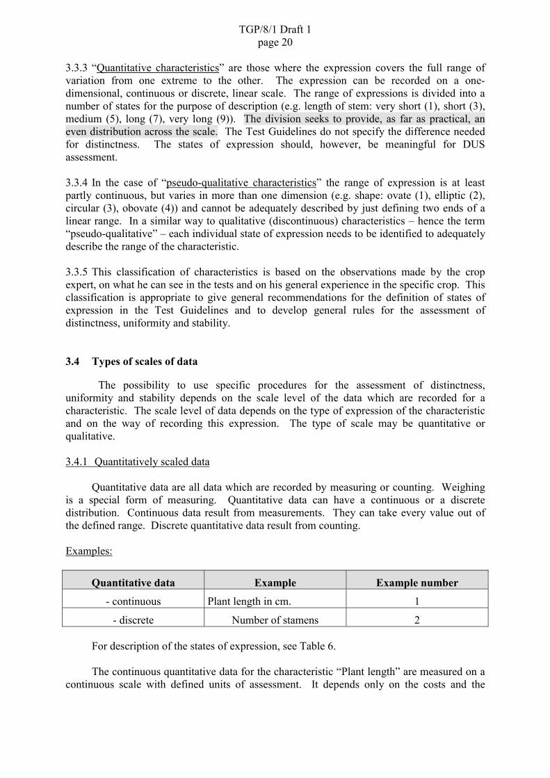
3.3.3 “Quantitative characteristics” are those where the expression covers the full range ofvariation from one extreme to the other. The expression can be recorded on a one-dimensional, continuous or discrete, linear scale. The range of expressions is divided into anumber of states for the purpose of description (e.g. length of stem: very short (1), short (3),medium (5), long (7), very long (9)). The division seeks to provide, as far as practical, aneven distribution across the scale. The Test Guidelines do not specify the difference neededfor distinctness. The states of expression should, however, be meaningful for DUSassessment.
3.3.4 In the case of “pseudo-qualitative characteristics” the range of expression is at leastpartly continuous, but varies in more than one dimension (e.g. shape: ovate (1), elliptic (2),circular (3), obovate (4)) and cannot be adequately described by just defining two ends of alinear range. In a similar way to qualitative (discontinuous) characteristics – hence the term“pseudo-qualitative” – each individual state of expression needs to be identified to adequatelydescribe the range of the characteristic.
3.3.5 This classification of characteristics is based on the observations made by the cropexpert, on what he can see in the tests and on his general experience in the specific crop. Thisclassification is appropriate to give general recommendations for the definition of states ofexpression in the Test Guidelines and to develop general rules for the assessment ofdistinctness, uniformity and stability.
3.4 Types of scales of data
The possibility to use specific procedures for the assessment of distinctness,uniformity and stability depends on the scale level of the data which are recorded for acharacteristic. The scale level of data depends on the type of expression of the characteristicand on the way of recording this expression. The type of scale may be quantitative orqualitative.
3.4.1 Quantitatively scaled data
Quantitative data are all data which are recorded by measuring or counting. Weighingis a special form of measuring. Quantitative data can have a continuous or a discretedistribution. Continuous data result from measurements. They can take every value out ofthe defined range. Discrete quantitative data result from counting.
Examples:
Quantitative data Example Example number
- continuous Plant length in cm. 1
- discrete Number of stamens 2
For description of the states of expression, see Table 6.
The continuous quantitative data for the characteristic “Plant length” are measured on acontinuous scale with defined units of assessment. It depends only on the costs and the

TGP/8/1 Draft 1page 21
necessity to get any value in cm or in mm. A change of unit of measurement e.g. from cminto mm is only a question of precision and not a change of type of scale.
The discrete quantitative data of the characteristic “Number of stamens “ are assessedby counting (1, 2, 3, 4, and so on). The distances between the neighbouring units ofassessment are constant and for this example equal to 1. There are no real values betweentwo neighbouring units but it is possible to compute an average which falls between thoseunits.
In biometrical terminology, quantitative scales are also designated as metric scales. Asynonym for metric scale is cardinal scale. Quantitative scales can be subdivided into ratioscales and interval scales.
3.4.1.1 Ratio scale
A ratio scale is a quantitative scale with a defined absolute zero point. There is always aconstant non-zero distance between two adjacent expressions. Ratio-scaled data may becontinuous or discrete.
The absolute zero point:
The definition of an absolute zero point makes it possible to define meaningful ratios.This is a requirement for the construction of index numbers (e.g. the ratio of length to width).An index is the combination of at least two characteristics. In the General Introduction, thisspecial case is defined as a combined characteristic.
It is also possible to calculate ratios between the expression of different varieties. Forexample, in the characteristic ‘Plant length’ assessed in cm, there is a lower limit for theexpression which is ‘0 cm’ (zero). It is possible to calculate the ratio of length of plant ofvariety ‘A’ to length of plant of variety ‘B’ by division:
Length of plant of variety ‘A’ = 80 cmLength of plant of variety ‘B’ = 40 cm
Ratio = Length of plant of variety ‘A’ / Length of plant of variety ‘B’ = 80 cm / 40 cm = 2.
So it is possible in this example to state that plant ‘A’ is double the length of plant ‘B’.The existence of an absolute zero point ensures an unambiguous ratio.
The ratio scale is the highest classification of the scales (Table 2). That means that ratioscaled data include the highest information about the characteristic and it is possible to usemany statistical procedures (Chapter 7).
The examples 1 and 2 (Table 6) are examples for characteristics with ratio scaled data.

TGP/8/1 Draft 1page 22
3.4.1.2 Interval scale
An Interval scale is a quantitative scale without a defined absolute zero point. There isalways a constant non-zero distance between two adjacent expressions. Interval scaled datamay be distributed continuously or discretely.
An example for a discrete interval scaled characteristic is ‘Time of beginning offlowering’ measured as date which is given in section 3.4.1 (see also example 6 in Table 6).This characteristic is defined as the number of days from April 1. The definition is useful butarbitrary and April 1 is not a natural limit. It would also be possible to define thecharacteristic as the number of days from January 1.
It is not possible to calculate a meaningful ratio between two varieties which should beillustrated with the following example:
Variety ‘A’ begins to flower on May 30 and variety ‘B’ on April 30
Case I) Number of days from April 1 of variety ‘A’ = 60 Number of days from April 1 of variety ‘B’ = 30
Number of days from April 1 of variety ‘A’ 60 daysRatioI = ----------------------------------------------------- = --------- = 2
Number of days from April 1 of variety ‘B 30 days
Case II) Number of days from January 1 of variety ‘A’ = 150 Number of days from January 1 of variety ‘B’ = 120
Number of days from January 1 of variety ‘A’ 150 daysRatioII = ------------------------------------------------------- = ----------- = 1.25
Number of days from January 1 of variety ‘B 120 days
RatioI = 2 > 1.25 = RatioII
It is impossible to state that the time of flowering of variety ‘A’ is twice that of variety‘B’. The ratio depends on the choice of the zero point of the scale. This kind of scale isdefined as an “Interval scale”: a quantitative scale without a defined absolute zero point.
The interval scale is lower classified than the ratio scale (Table 2). Fewer statisticalprocedures can be used with interval scaled data than with ratio scaled data (see section 3.7).The interval scale is theoretically the minimum scale level to calculate arithmetic meanvalues.
3.4.2. Qualitatively scaled data
Qualitatively scaled data are data which can be arranged in different discrete qualitativecategories. Usually they result from visual assessment. Subgroups of qualitative scales areordinal and nominal scales.

TGP/8/1 Draft 1page 23
3.4.2.1 Ordinal scale
Ordinally scaled data are qualitative data of which discrete categories can be arranged inan ascending or descending order. They result from visually assessed quantitativecharacteristics.
Example:
Qualitative data Example Example number
- ordinal Intensity of anthocyanin 3
For description of the states of expressions, see Table 6.
An ordinal scale consists of numbers which correspond to the states of expression of thecharacteristic (notes). The expressions vary from one extreme to the other and thus they havea clear logical order. It is not possible to change this order, but it is not important whichnumbers are used to denote the categories. In some cases ordinal data may reach the level ofdiscrete interval scaled data or of discrete ratio scaled data (Chapter 6).
The distances between the discrete categories of an ordinal scale are not exactly knownand not necessarily equal. Therefore, an ordinal scale does not fulfil the condition to calculatearithmetic mean values, which is the equality of intervals throughout the scale.
The ordinal scale is lower classified than the interval scale (Table 2). Less statisticalprocedures can be used for ordinal scale than for each of the higher classified scale data (seesection 3.7).
3.4.2.2 Nominal scale
Nominal scaled qualitative data are qualitative data without any logical order of thediscrete categories.
Examples:
Qualitative data Example Example number
- nominal Sex of plant 4
- nominal with two states Leaf blade: variegation 5
For description of the states of expressions, see Table 6.
A nominal scale consists of numbers which correspond to the states of expression of thecharacteristic, which are referred to in the Test Guidelines as notes. Although numbers areused for designation there is no inevitable order for the expressions and so it is possible toarrange them in any order.
Characteristics with only two categories (dichotomous characteristic) are a special formof nominal scales.

TGP/8/1 Draft 1page 24
The nominal scale is the lowest classification of the scales (Table 2). Few statisticalprocedures are applicable for evaluations (Chapter 7).
The different types of scales are summarised in the following table.
Table 2: Types of scales and scale levels
Type of scale Description Distribution Data recording ScaleLevel
Continuous AbsoluteMeasurementsratio
constantdistances withabsolute zeropoint
Discrete Counting
High
Continuous Relativemeasurements
quantitative(metric) interval constant
distanceswithoutabsolute zeropoint
Discrete Date
qualitativewithunderlyingquantitativevariable
ordinal
Orderedexpressionswith varyingdistances
Discrete Visually assessednotes
qualitative nominal No order, nodistances
Discrete Visually assessednotes
Low
From the statistical point of view a characteristic is only considered at the level of datawhich has been recorded, whether for analysis or for describing the expression of thecharacteristic. Therefore, characteristics with quantitative data are denoted as quantitativecharacteristics and characteristics with ordinal and nominal scaled data as qualitativecharacteristics.
3.5 Scale levels for variety description
The description of varieties is based on the states of expression (notes) which are givenin the Test Guidelines for the specific crop. In the case of visual assessment, the notes fromthe Test Guidelines are usually used for recording the characteristic as well as for theassessment of DUS. As outlined in chapter 4, the notes are distributed on a nominal orordinal scale. For measured or counted characteristics, DUS assessment is based on therecorded values and the recorded values are transformed into states of expression only for thepurpose of variety description.
3.6 Relation between types of expression of characteristics and scale levels of data
3.6.1 Records taken for the assessment of qualitative characteristics are distributed on anominal scale, for example “Sex of plant”, “Leaf blade: variegation” (Table 6, examples 4and 5).
3.6.2 For quantitative characteristics the scale level of data depends on the method ofassessment. They can be recorded on a quantitative or ordinal scale. For example, “Length of

TGP/8/1 Draft 1page 25
plant” can be recorded by measurements resulting in ratio scaled continuous quantitative data.However, visual assessment on a 1 to 9 scale may also be appropriate. In this case, therecorded data are qualitatively scaled (ordinal scale) because the size of intervals between themidpoints of categories is not exactly the same.
Remark: In some cases visually assessed data on quantitative characteristics may be handledas measurements. The possibility to apply statistical methods for quantitative datadepends on the precision of the assessment and the robustness of the statisticalprocedures. In the case of very precise visually assessed quantitative characteristicsthe usually ordinal data may reach the level of discrete interval scaled data or ofdiscrete ratio scaled data.
3.6.3 A pseudo-qualitative type of characteristic is one in which the expression varies in morethan one dimension. The different dimensions are combined in one scale. At least onedimension is quantitatively expressed. The other dimensions may be qualitatively expressedor quantitatively expressed. The scale as a whole has to be considered as a nominal scale(e.g. “Shape”, “Flower color”; Table 6, examples 7 and 8).
3.6.4 In the case of using the off-type procedure for the assessment of uniformity the recordeddata are nominally scaled. The records fall into two qualitative classes: plants belonging tothe variety (true-types) and plants not belonging to the variety (off-types). The type of scaleis the same for qualitative, quantitative and pseudo-qualitative characteristics.
3.6.5 The relation between the type of characteristics (process level 1) and the type of scale ofdata recorded for the assessment of distinctness and uniformity is described in Table 3. Aqualitative characteristic is recorded on a nominal scale for distinctness (state of expression)and for uniformity (true-types vs. off-types). Pseudo-qualitative characteristics are recordedon a combined scale for distinctness (state of expression) and on a nominal scale foruniformity (true-types vs. off-types). Quantitative characteristics are recorded on an ordinal,interval or ratio scale for the assessment of distinctness depending on the characteristic andthe method of assessment. If the records are taken from single plants the same data may beused for the assessment of distinctness and uniformity. If distinctness is assessed on the basisof a single record of a group of plants, uniformity has to be judged with the off-typeprocedure (nominal scale).

TGP/8/1 Draft 1page 26
Table 3: Relation between type of characteristic and type of scale of assessed data
Type of characteristic (level 1)Procedure Type of scale(level 2) Distribution Quantitative Pseudo-qualitative Qualitative
Continuous ・ratio Discrete ・Continuous ・interval Discrete ・
ordinal Discrete ・
combined Discrete ・Dis
tinct
ness
nominal Discrete ・
Continuous ・ratioDiscrete ・Continuous ・intervalDiscrete ・
ordinal Discrete ・combined Discrete ・U
nifo
rmity
nominal Discrete ・ ・ ・
3.7 Relation between method of observation of characteristics, scale levels of data andrecommended statistical procedures
3.7.1 The scale level of data and the way of observation of characteristics are most importantconditions for the application of different statistical procedures. There are four possible waysto observe characteristics (see document TGP/7 “Development of Test Guidelines”):
MG: single record for a group of plants or parts of plants based on measurement(s)MS: records for a number of single, individual plants or parts of plants obtained by
measurementVG: single record for a group of plants or parts of plants based on visual observation(s)VS: records for a number of single, individual plants or parts of plants obtained by
visual observation.
3.7.2 The observation method depends primarily on the variation within and betweenvarieties and affects the choice of the statistical method. All of the four observation methodsmay be relevant for the assessment of distinctness. For the assessment of uniformityobservations must be done on individual plants. Consequently only MS or VS areappropriate. The indication of the method of observation of characteristics in the TestGuidelines refers only to the assessment of distinctness.
3.7.3 Established statistical procedures can be used for the assessment of distinctness anduniformity considering the scale level and some further conditions such as the degree offreedom or unimodality (Tables 4 and 5).
3.7.4 The relation between the expression of characteristics and the scale levels of data for theassessment of distinctness and uniformity is summarized in Table 6.

TGP/8/1 Draft 1page 27
Table 4: Statistical procedures for the assessment of distinctness
Type ofscale
Distribu-tion
Observa-tionmethod
Procedure1) and further Conditions
Refe-rencedocument
continuousratio
discrete
continuousinterval
discrete
MSMG(VS) 2)
R: COY-D Normal distribution, df >=20
R: long term LSD Normal distribution, df<20
NR-P: 2 out of 3 method (LSD 1%) Normal distribution, df>=20
TGP/9
ordinal discrete VG
VS
R: minimum distance>=1
NR-D: threshold model
TGP/9
TWC/14/12
Combina-tion ofordinal orordinalandnominalscales
discrete VG(VS) 3)
R: state-by-state-comparison TGP/9
nominal discrete VG(VS) 3)
R: each state-is clearly different from the other
TGP/9
1) R recommendedNR-P not recommended (previous method)NR-D not recommended (method under development)
2) see remark in Chapter 63) normally VG but VS would be possible

TGP/8/1 Draft 1page 28
Table 5: Statistical procedures for the assessment of uniformity
Type ofscale
Distribu-tion
observa-tionmethod
Procedure1) andFurther Conditions
Refe-rencedocument
continuousratio
discrete
continuousinterval
discrete
MS
MS
VS
R: COY-U Normal distributionNR-P: 2 out of 3 method (s2
c<=1.6s2s))
Normal distributionNR-D: LSD for untransformed percentage ofoff-types
TGP/10.3.1
ordinal discrete VS NR-D: threshold model TWC/14/12
Combina-tion ofordinal orordinalandnominalscales
discrete There is no case where uniformity is assessedon combined scaled data
nominal discrete VS R: off-type procedure for dichotomous(binary) data
TGP/10.3.2
1) R recommendedNR-P not recommended (previous method)NR-D not recommended (method under development)

TGP/8/1 Draft 1page 29
Table 6: Relation between expression of characteristics and scale levels of data for the assessment of distinctness and uniformity
Distinctness UniformityExample Name of
characteristicUnit ofassess-ment
Description(states of
expression)
Type of scale Unit ofassess-ment
Description(states of
expression)
Type of scale
cm assessment in cmwithout digits afterdecimal point
ratio scaledcontinuousquantitative data
1 Length of plant cm assessment in cmwithout digits afterdecimal point
ratio scaled continuousquantitative data
True-type
Off-type
Number of plantsbelonging to thevarietyNumber of off-types
nominally scaledqualitative data
2 Number ofstamens
counts 1, 2, 3, ... , 40,41, ... ratio scaled discretequantitative data
counts 1, 2, 3, ... , 40,41, ... ratio scaled discretequantitative data
3 Intensity of 1 very lowanthocyanin 2 very low to low
3 low4 low to medium5 medium6 medium to high7 high8 high to very high9 very high
ordinally scaledqualitative data (withan underlyingquantitative variable)
True-type
Off-type
Number of plantsbelonging to thevarietyNumber of off-types
nominally scaledqualitative data
4 Sex of plant 1234
dioecious femaledioecious malemonoeciousunisexualmonoecioushermaphrodite
nominally scaledqualitative data
True-type
Off-type
Number of plantsbelonging to thevarietyNumber of off-types
nominally scaledqualitative data

TGP/8/1 Draft 1page 30
Distinctness UniformityExample Name of
characteristicUnit ofassess-ment
Description(states of
expression)
Type of scale Unit ofassess-ment
Description(states of
expression)
Type of scale
5 Leaf blade:variegation
19
absentpresent
nominally scaledqualitative data
True-type
Off-type
Number of plantsbelonging to thevarietyNumber of off-types
nominally scaledqualitative data
date e.g. May 21, 51st dayfrom April 1
interval scaled discretequantitative data
6 Time ofbeginning offlowering
date e.g. May 21, 51st dayfrom April 1
interval scaled discretequantitative data
True-type
Off-type
Number of plantsbelonging to thevarietyNumber of off-types
nominally scaledqualitative data
7 Shape 1 deltate True-type Number of plants nominally scaled2 ovate belonging to the qualitative data3 elliptic variety4567
obovateobdeltatecircularoblate
combination of ordinaland nominal scaleddiscrete qualitative data
Off-type Number of off-types
8 Flower color 12345678910
dark redmedium redlight redwhitelight bluemedium bluedark bluered violetvioletblue violet
combination of ordinaland nominal scaleddiscrete qualitative data
True-type
Off-type
Number of plantsbelonging to thevarietyNumber of off-types
nominally scaledqualitative data

TGP/8/1 Draft 1page 31
SECTION 4: VALIDATION OF DATA AND ASSUMPTIONS
4.1 Introduction
Statistical analyses are carried out in order to assist the crop expert when assessingcandidate varieties for distinctness, uniformity and stability. In section 2, “ExperimentalDesign Practices”, aspects of designing the experiments in which the data are recorded arediscussed. In section 3, “Types of Characteristics and Their Scale Levels”, it is shown thatthe choice of which statistical methods to use depends on the type of characteristic, its scalelevel, and whether distinctness or uniformity is considered. In section 5, “Statistical Methodsfor DUS Examination”, the statistical methods are described. The statistical methods arebased on some theory and in order to ensure that the results can be trusted the assumptionsbehind the theory have to be met - at least approximately. The purpose of this section is todescribe the assumptions behind the most common statistical methods used in DUS testingand to show how these assumptions may be validated. It is important to note that the COYDand COYU methods for used quantitative characteristics are based on variety means per yearfor COYD, and variety means of the (logarithm of the) between-plants standard deviation peryear for COYU. Some methods for checking the data are described in section 4.2 “Check onData Quality” below. In section 4.3, “Assumptions”, the assumptions underlying the analysisof variance methods are given and in section 4.4, “Validation”, some methods for evaluatingthese assumptions are given. The assumptions and methods of validation are described herefor the analyses of single experiments (randomized blocks). However, the principles are thesame when analyzing data from several experiments over years. Instead of plot means, theanalyses are then carried out on variety means per year (and blocks then become equivalent toyears). The methods described here are intended for quantitative characteristics, but some ofthe methods may also be used for checking qualitative characteristics on the ordinal scale.The different types of characteristics are defined in document TGP/8.3. Throughout thissection data of ‘Leaf: Length’ (in mm) are used of an experiment laid out in 3 blocks of 26plots with 20 plants per plot. Within each block, 26 different oil seed rape varieties wererandomly assigned to each plot.
4.2 Check on data quality (before doing analyses)
4.2.1 In order to avoid mistakes in the interpretation of the results the data should always beinspected so that the data are logically consistent and not in conflict with prior informationabout the ranges likely to arise for the various characteristics. This inspection can be donemanually (usually visually) or automatically.
4.2.2 Table 1 shows an extract of some recordings for 10 plants from a plot of field peas. For‘Seed: shape’ the notes are visually scored on a scale with values 1, 2, 3, 4, 5 or 6. For ‘Stem:length’ the measurements are in cm and from past experience it is known that the length inmost cases will be between 40 and 80 cm. The ‘Stipule: length’ is measured in mm and willin most cases be between 50 and 90 mm. The table shows 3 types of mistakes whichoccasionally occur when making manual recordings: for plant 4, ‘Seed: shape’ the recordedvalue, 7, is not among the allowed notes and must, therefore, be due to a mistake. It might becaused by a misreading a hand-written “1”. The ‘Stem: length’ of plant 6 is outside theexpected range and could be caused by changing the order of the figures, so 96 has beenkeyed instead of 69. The ‘Stipule: length’ of 668 mm is clearly wrong. It might be caused by

TGP/8/1 Draft 1page 32
accidentally repeating the figure 6 twice. In all cases a careful examination has to be carriedout in order to find out what the correct values should be.
Table 1 Extract of recording sheet for field peas
Plant no Seed: shape(UPOV 1)
Stem: length(UPOV 12)
Stipule: length(UPOV 31)
1 1 43 802 2 53 793 1 50 724 7 43 6685 2 69 726 1 96 727 1 51 708 2 64 639 1 44 6210 2 49 62
4.2.3 Examination of frequency distributions of the characteristics to look for small groups ofdiscrepant observations.
Figure 1. Box-plot for Leaf Length of 26 oil seed rape
Figure 1. Box-plot for Leaf Length of 26 varieties of oil seed rape

TGP/8/1 Draft 1page 33
4.2.4 Examination of scatter plots of pairs of characteristics likely to be highly related. Thismay often detect discrepant observations very efficiently.
4.2.5 Other types of plot may also be used to validate the quality of the data. A so-calledBox- plot is an efficient way to get an overview of the data. In a Box-plot a box is drawn foreach group (plot or variety). In Figure 1, all 60 Leaf Lengths of each of the 26 varieties aretaken together. (If there are large block differences a better Box-plot can be produced bytaking the differences with respect to the plot mean). The box shows the range for the largestpart of the individual observations (usually 75%). A horizontal line through the box and asymbol indicates the median and mean, respectively. At each end of the box, vertical linesare drawn to indicate the range of possible observations outside the box, but within areasonable distance (usually 1.5 times the height of the box). Finally, observations moreextreme than that are shown individually. In Figure 1, it is seen that one observation ofvariety 13 is clearly much larger than the remaining observations of that variety. Also it isseen that variety 16 has large leaf lengths and that about 4 observations are relatively far fromthe mean. Among other things that can be seen from the figure are the variability and thesymmetry of the distribution. So it can be seen that the variability of variety 15 is relativelylarge and that the distribution is slightly skewed for this variety (as the mean and median arerelatively far apart).
4.2.6 When discrepant observations are found, the next important step will be to find out whythe observations are deviating. In some cases it may be possible to go back to the field and tocheck if the plant or plot is damaged by external factors (e.g. rabbits) or a measurementmistake has occurred. In the last case a correction is possible. In other cases, it may benecessary to look in previous notes (or on other measurements from the same plant/plot) inorder to find the reason for the discrepant observation. Generally observations should only beremoved when there are good reasons. When in doubt it is recommended to discuss theproblem with a statistician.
4.3 Assumptions
4.3.1 First of all it is very important to design experiments in a proper way. The mostimportant assumptions of analysis of variance methods are:
� independent observations� variance homogeneity� additivity of block and variety effects for a randomized block design and
additivity of year and variety effects for COYD.� normally distributed observations (residuals)
4.3.2 In addition, one could state that there should be no mistakes in the data. However, mostmistakes (at least the largest) will usually also mean that the observations are not normallydistributed and that they have different variances.
4.3.3 The assumptions mentioned here are most important when the statistical methods areused to test hypotheses. When statistical methods are used only to estimate effects (means),the assumptions are less important and the assumption of normal distributed observations isnot necessary.

TGP/8/1 Draft 1page 34
Independent observations
4.3.4 This is a very important assumption. It means that no records may depend on otherrecords in the same analysis (dependence between observations may be built into the model,but this is not so in the COYD and COYU or other UPOV recommended methods).Dependency may be caused e.g. by competitions between neighbouring plots, by lack ofrandomisation or by improper randomisation. More details on ensuring independence ofobservations may be found in document section 2 “Experimental Design Practices.”
Variance homogeneity
4.3.5 Variance homogeneity means that the variance of all observations should be identicalapart from random variation. Typical deviations from the assumption of variancehomogeneity fall most often into one of the following two groups:
� The variance depends on the mean, e.g. the larger the mean value the larger thestandard deviation is. In this case the data may often be transformed such that thevariances on the transformed scale may be approximately homogeneous. Some typicaltransformations of characteristics are: the logarithmic transformation (where thestandard deviation is approximately proportional to the mean), the square-roottransformation (where the variance is approximately proportional to the mean, e.g.counts), and the angular transformation (where the variance is low at both ends of thescale and higher in between, typical for percentages).
� The variance depends on e.g. variety, year or block. If the variances depend on suchvariables in a way that is not connected to the mean value, it is not possible to obtainvariance homogeneity by transformation. In such cases it might be necessary either touse more complicated statistical methods that can take unequal variances into accountor to exclude the group of observations with deviant variances (if only a fewobservations have deviant variances). To illustrate the seriousness of varianceheterogeneity: imagine a small trial with 10 varieties where varieties A, B, C, D, E, F,G and H each have a variance of 5, whereas varieties I and J each have a variance of10. The real probability of detecting differences between these varieties when, in fact,they have the same mean is shown in Table 2. In Table 2, the variety comparisons arebased on the pooled variance as is normal in traditional ANOVA. If they arecompared using the 1% level of significance, the probability that the two varieties witha variance of 10 become significantly different from each other is almost 5 timeslarger (4.6%) than it should be. On the other hand, the probability of significantdifferences between two varieties with a variance of 5 decreases to 0.5%, when itshould be 1%. This means that it becomes too difficult to detect differences betweentwo varieties with small variances and too easy to detect differences between varietieswith large variances.

TGP/8/1 Draft 1page 35
Table 2. Real probability of significant difference between two identical varieties in the case where variancehomogeniety is assumed but not fulfilled (varieties A to H have a variance of 5 and varieties I and J have avariance of 10.)
Formal test of significance levelComparisons,variety names 1% 5%A and B 0.5% 3.2%A and I 2.1% 8.0%I and J 4.6% 12.9%
Normal distributed observations
4.3.6 The residuals (see section 5 “Statistical Methods for DUS Examination”) should beapproximately normally distributed. The ideal normal distribution means that the distributionof the data is symmetric around the mean value and with the characteristic bell-shaped form(see Figure 2). If theresiduals are notapproximatelynormally distributed,the actual level ofsignificance maydeviate from thenominal level. Thedeviation may be inboth directionsdepending on theway the actualdistribution of theresiduals deviatesfrom the normaldistribution.However, deviationfrom normality isusually not as seriousas deviations from the previous two assumptions.
Additivity of block and variety effects
4.3.7 The effects of blocks and varieties are assumed to be additive because the error term isthe sum of random variation and the interaction between block and variety. (For a formaldescription of the model see document section 5 Two-way ANOVA paragraph 5.1.7). Thismeans that the effect of a given variety is the same in all blocks. This is demonstrated inTable 3 where plot means of artificial data (of Leaf Length in mm) are given for two smallexperiments with three blocks and four varieties. In experiment I, the effects of blocks andvarieties are additive because the differences between any two varieties are the same in allblocks, e.g. the differences between variety A and B are 4 mm in all three blocks. Inexperiment II, the effects are not additive, e.g. the differences between variety A and B are 2,2 and 8 mm in the three blocks.
Figure 2. Histogram for normal distributed data with the ideal normaldistribution shown as a curve

TGP/8/1 Draft 1page 36
Table 3. Artificial plot means of Leaf Length in mm from two experiments showing additive block and varietyeffects (left) and non-additive block and variety effects (right)
Experiment I Experiment IIBlock BlockVariety
1 2 3Variety
1 2 3A 240 242 239 A 240 242 239B 244 246 243 B 242 244 247C 245 247 244 C 246 244 243D 241 243 240 D 241 242 241
Figure 3. Artificial plot means from two experiments showing additive block and variety effects (left) and non-additive block and variety effects (right) using same data as in table 2
4.3.8 In Figure 3 the same data are presented graphically. Plotting the means versus blocknumbers and joining the observations from the same varieties by straight lines produces thegraphs. Plotting the means versus variety names and joining the observations from the sameblocks could also have been used (and may be preferred especially if many varieties are to beshown in the same figure). The assumption on additivity is fulfilled if the lines for thevarieties are parallel (apart from random variation). As there is just a single data value foreach variety in each block, it is not possible to separate interaction effects and randomvariation. So in practice the situation is not as nice and clear as here because the effects maybe masked by random variation.
4.4 Validation
4.4.1 The purpose of validation is partly to check that the data are without mistakes and thatthe assumptions underlying the statistical analyses are fulfilled.
4.4.2 There are different methods to use when validating the data. Some of these are:
� look through the data� produce plots to verify the assumptions� make formal statistical tests for the different types of assumptions. In the literature
several methods to test for outliers, variance homogeneity, additivity and normalitymay be found. Such methods will not be mentioned here partly because many ofthese depend on assumptions that do not affect the validity of COYD and COYUseriously and partly because the power of such methods depends heavily on the
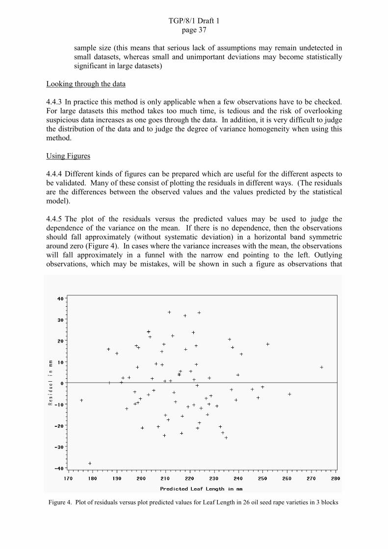
TGP/8/1 Draft 1page 37
sample size (this means that serious lack of assumptions may remain undetected insmall datasets, whereas small and unimportant deviations may become statisticallysignificant in large datasets)
Looking through the data
4.4.3 In practice this method is only applicable when a few observations have to be checked.For large datasets this method takes too much time, is tedious and the risk of overlookingsuspicious data increases as one goes through the data. In addition, it is very difficult to judgethe distribution of the data and to judge the degree of variance homogeneity when using thismethod.
Using Figures
4.4.4 Different kinds of figures can be prepared which are useful for the different aspects tobe validated. Many of these consist of plotting the residuals in different ways. (The residualsare the differences between the observed values and the values predicted by the statisticalmodel).
4.4.5 The plot of the residuals versus the predicted values may be used to judge thedependence of the variance on the mean. If there is no dependence, then the observationsshould fall approximately (without systematic deviation) in a horizontal band symmetricaround zero (Figure 4). In cases where the variance increases with the mean, the observationswill fall approximately in a funnel with the narrow end pointing to the left. Outlyingobservations, which may be mistakes, will be shown in such a figure as observations that
Figure 4. Plot of residuals versus plot predicted values for Leaf Length in 26 oil seed rape varieties in 3 blocks

TGP/8/1 Draft 1page 38
clearly have escaped from the horizontal band formed by most other observations. In theexample used in figure 4, no observations seem to be outliers (the value at the one bottom leftcorner where the residual is about -40 mm may at first glance look so, but severalobservations have positive values of the same numerical size). Here it is important to notethat an outlier is not necessarily a mistake and also that a mistake will not necessarily show upas an outlier.
4.4.6 The residuals can also be used to form a histogram, like Figure 2, from which theassumption about the distribution can be judged.
4.4.7 The range (maximum value minus minimum value) or standard deviation for each plotmay be plotted versus some other variables such as the plot means, variety number or plotnumber. Such figures (Figure 5) may be useful to find varieties with an extremely largevariation (all plots of the variety with a large value) or plots where the variation is extremelylarge (maybe caused by a single plant). It is clearly seen that the range for one of variety 13’splots is much higher than in the other two plots. Also the range in one of variety 3’s plotsseems to be relatively large.
4.4.8 A figure with the plot means (or variety adjusted means) versus the plot number can beused to find out whether the characteristic depends on the location in the field (Figure 6).This, of course, requires that the plots are numbered such that the numbers indicate therelative location. In the example shown in Figure 6, there is a clear trend showing that theleaf length decreases slightly with plot number. However most of the trend over the area used
Figure 5. Differences between minimum and maximum of 20 leaf lengths for 3 plots versus oil seed rape varietynumber

TGP/8/1 Draft 1page 39
for the trial will - in this case - be explained by differences between blocks (plot 1-26 is block1, plot 27-52 is block 2 and plot 53-78 is block 3).
4.4.9 The plot means can also be used to form a figure where the additivity of block andvariety effects can be visually checked at (see Figure 3).
4.4.10 Normal Probability Plots (Figure 7). This type of graph is used to evaluate towhat extent the distribution of the variable follows the normal distribution. The selectedvariable will be plotted in a scatter plot against the values “expected from the normaldistribution.” The standard normal probability plot is constructed as follows. First, theresiduals (deviations from the predictions) are rank ordered. From these ranks the programcomputes the expected values from the normal distribution, hereafter called z-values. Thesez-values are plotted on the X-axis in the plot. If the observed residuals (plotted on the Y-axis)are normally distributed, then all values should fall onto a straight line. If the residuals arenot normally distributed, then they will deviate from the line. Outliers may also becomeevident in this plot. If there is a general lack of fit, and the data seem to form a clear pattern(e.g. an S shape) around the line, then the variable may have to be transformed in some way.
Figure 6. Plot means of 20 Leaf Lengths versus plot numbers
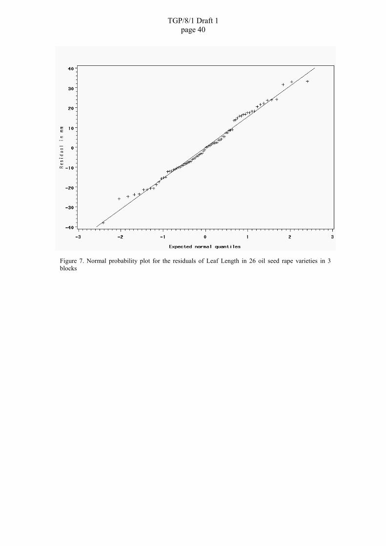
TGP/8/1 Draft 1page 40
Figure 7. Normal probability plot for the residuals of Leaf Length in 26 oil seed rape varieties in 3blocks

TGP/8/1 Draft 1page 41
SECTION 5: STATISTICAL METHODS FOR DUS EXAMINATION
5.1 Analysis of variance
5.1.1 Introduction
5.1.1.1 The analysis of variance (ANOVA) of data from a designed experiment has twopurposes. Firstly it subdivides the data’s total variation into separate components with eachcomponent representing a different source of variation, so that the relative importance of thedifferent sources can be assessed. Secondly it provides an estimate of the random variation inthe data. This may be used as an estimate of precision when comparing means calculated fromthe data.
5.1.1.2 ANOVA can take many forms. Just two forms will be considered in detail here.These are the two forms which arise as part of the statistical techniques used in COY. Attheir simplest, both operate on an n�m table of data. They are the:-
– Two-way ANOVA, e.g. as used in the analysis of variety-by-year means for acharacteristic for v varieties grown in each of y years in the Combined Over YearsDistinctness (COYD) (see appendix A4) criterion. The paired t-test is a specialcase of two-way ANOVA.
– One-way ANOVA, e.g. as used in the analysis of variety-by-year adjustedlog(SD+1)’s (a measure of uniformity) for a characteristic for v reference varietiesgrown in each of y years in the Combined Over Years Uniformity (COYU)criterion.
5.1.1.3 The particular form an ANOVA takes depends on the origins of the data. Thisdetermines the model for the data, i.e. what factors are likely to cause the data to vary, whichin turn determines what components the total variation is divided into, and hence the form ofthe ANOVA.
5.1.2 Two-way ANOVA
5.1.2.1 The data model
5.1.2.1.1 In two-way ANOVA, the n�m table of data corresponds to nm data valuesclassified by two factors: Factor 1 with m levels and Factor 2 with n levels. Usually, only oneof the factors will be of interest while the other will be present simply because it explainsvariability in the data. For example (Example A), each data value might be the mean over allplants in a plot for a characteristic from a trial with vb plots laid out in b blocks (Factor 1) of vvarieties (Factor 2), the factor of interest.
Example A: data from a trial with v varieties and b blocksBlock 1 Block 2 Block 3 � Block b
Variety 1 - - - � -Variety 2 - - - � -Variety 3 - - - � -
� � � � � �
Variety v - - - � -vb data values
mean of all plants in the plot in block 2 with variety 3
mean of all plants inthe plot in block bwith variety 2
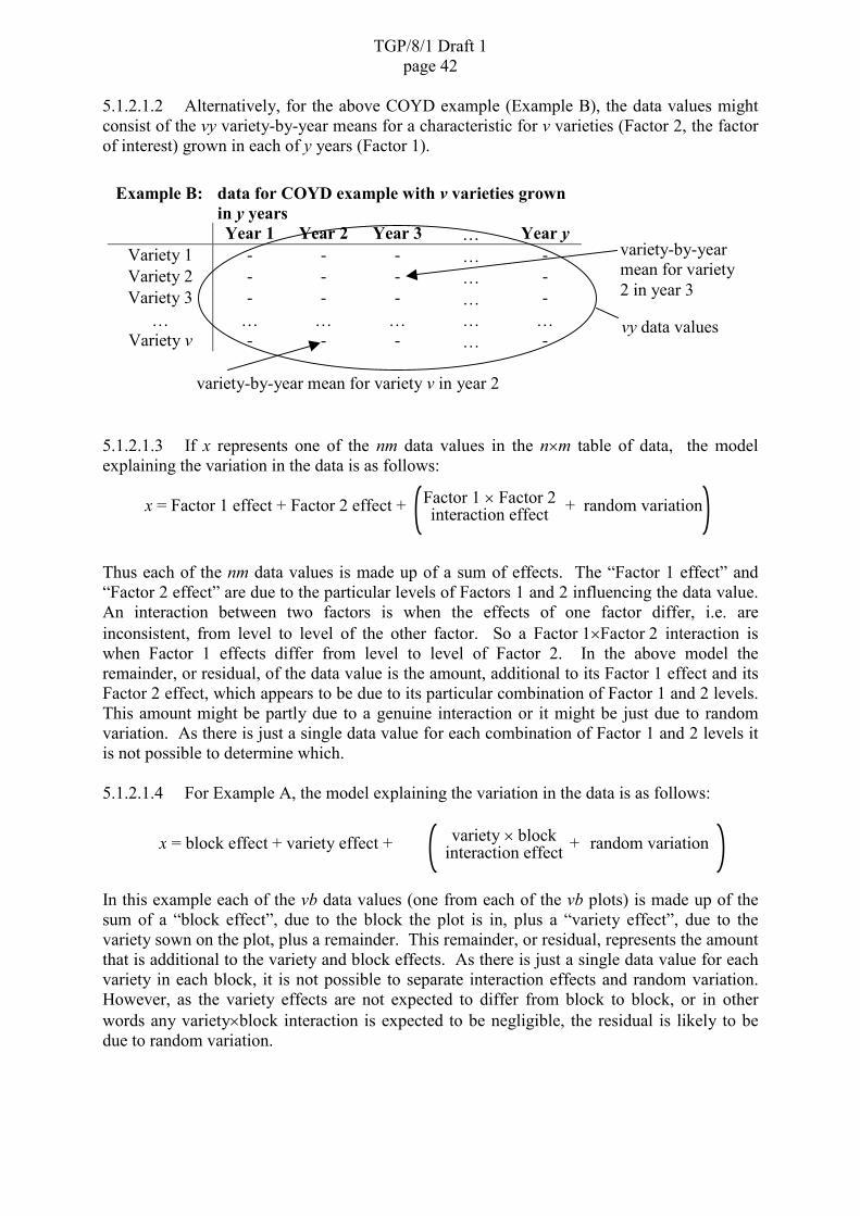
TGP/8/1 Draft 1page 42
5.1.2.1.2 Alternatively, for the above COYD example (Example B), the data values mightconsist of the vy variety-by-year means for a characteristic for v varieties (Factor 2, the factorof interest) grown in each of y years (Factor 1).
5.1.2.1.3 If x represents one of the nm data values in the n�m table of data, the modelexplaining the variation in the data is as follows:
Thus each of the nm data values is made up of a sum of effects. The “Factor 1 effect” and“Factor 2 effect” are due to the particular levels of Factors 1 and 2 influencing the data value.An interaction between two factors is when the effects of one factor differ, i.e. areinconsistent, from level to level of the other factor. So a Factor 1�Factor 2 interaction iswhen Factor 1 effects differ from level to level of Factor 2. In the above model theremainder, or residual, of the data value is the amount, additional to its Factor 1 effect and itsFactor 2 effect, which appears to be due to its particular combination of Factor 1 and 2 levels.This amount might be partly due to a genuine interaction or it might be just due to randomvariation. As there is just a single data value for each combination of Factor 1 and 2 levels itis not possible to determine which.
5.1.2.1.4 For Example A, the model explaining the variation in the data is as follows:
In this example each of the vb data values (one from each of the vb plots) is made up of thesum of a “block effect”, due to the block the plot is in, plus a “variety effect”, due to thevariety sown on the plot, plus a remainder. This remainder, or residual, represents the amountthat is additional to the variety and block effects. As there is just a single data value for eachvariety in each block, it is not possible to separate interaction effects and random variation.However, as the variety effects are not expected to differ from block to block, or in otherwords any variety�block interaction is expected to be negligible, the residual is likely to bedue to random variation.
Example B: data for COYD example with v varieties grownin y yearsYear 1 Year 2 Year 3
�Year y
Variety 1 - - - � -Variety 2 - - - � -Variety 3 - - - � -
� � � � � �
Variety v - - - � -vy data values
variety-by-year mean for variety v in year 2
variety-by-yearmean for variety2 in year 3
x = block effect + variety effect + + random variationvariety � blockinteraction effect
x = Factor 1 effect + Factor 2 effect + + random variationFactor 1 � Factor 2interaction effect

TGP/8/1 Draft 1page 43
5.1.2.1.3 For Example B (COYD), the model explaining the variation in the data is asfollows:
Here each of the vy variety-by-year means is made up of a sum of effects. The “year effect”is an amount due to the year the variety-by-year mean was recorded in. The year effectsmight or might not be the same for all years. The “variety effect” is an amount due to thevariety of the variety-by-year mean, and might or might not be the same for all varieties. Theremainder, or residual of the variety-by-year mean represents the amount that is additional toits variety effect and its year effect, which appears to be due to that particular variety in thatparticular year. This amount may be partly due to a genuine variety�year interaction effect orit may be just due to random variation caused by the means having been calculated fromdifferent plants grown on different plots, and possibly due to measurement error. As there isjust a single variety-by-year mean for each variety in each year it is not possible to distinguishbetween interaction effects and random variation.
5.1.2.2 The two-way analysis of variance table
5.1.2.2.1 Two-way ANOVA produces a table as follows:
Source of variationDegrees ofFreedom
Sum ofSquares
MeanSquare F-ratio
Factor 1 m - 1 - - -Factor 2 n - 1 - - -Residual (n - 1)(m - 1) - -
Total nm - 1 -
[As the ANOVA computations are likely to be done by computer, details are not given here.Details can be found at the following references: Dagnelie (1998 and 1981), Kala (2002),Mead et al. (1993), and Sokal and Rohlf (1995).]
5.1.2.2.2 For Example A, the two-way ANOVA table is as follows:
Source of variationDegrees ofFreedom
Sum ofSquares
MeanSquare F-ratio
Block b - 1 - - -Variety v - 1 - - -Residual (b - 1)(v - 1) - -
Total vb - 1 -
x = year effect + variety effect + + random variationvariety � yearinteraction effect
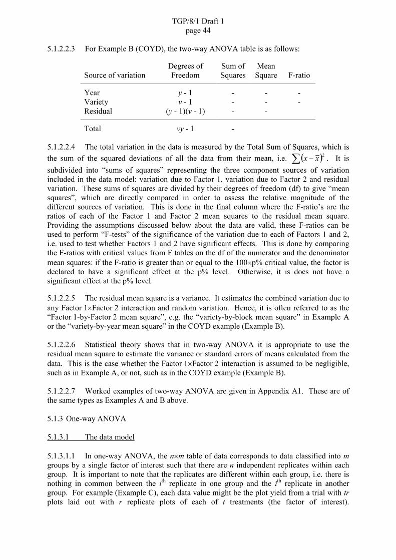
TGP/8/1 Draft 1page 44
5.1.2.2.3 For Example B (COYD), the two-way ANOVA table is as follows:
Source of variationDegrees ofFreedom
Sum ofSquares
MeanSquare F-ratio
Year y - 1 - - -Variety v - 1 - - -Residual (y - 1)(v - 1) - -
Total vy - 1 -
5.1.2.2.4 The total variation in the data is measured by the Total Sum of Squares, which isthe sum of the squared deviations of all the data from their mean, i.e. � �� �
2xx . It issubdivided into “sums of squares” representing the three component sources of variationincluded in the data model: variation due to Factor 1, variation due to Factor 2 and residualvariation. These sums of squares are divided by their degrees of freedom (df) to give “meansquares”, which are directly compared in order to assess the relative magnitude of thedifferent sources of variation. This is done in the final column where the F-ratio’s are theratios of each of the Factor 1 and Factor 2 mean squares to the residual mean square.Providing the assumptions discussed below about the data are valid, these F-ratios can beused to perform “F-tests” of the significance of the variation due to each of Factors 1 and 2,i.e. used to test whether Factors 1 and 2 have significant effects. This is done by comparingthe F-ratios with critical values from F tables on the df of the numerator and the denominatormean squares: if the F-ratio is greater than or equal to the 100�p% critical value, the factor isdeclared to have a significant effect at the p% level. Otherwise, it is does not have asignificant effect at the p% level.
5.1.2.2.5 The residual mean square is a variance. It estimates the combined variation due toany Factor 1�Factor 2 interaction and random variation. Hence, it is often referred to as the“Factor 1-by-Factor 2 mean square”, e.g. the “variety-by-block mean square” in Example Aor the “variety-by-year mean square” in the COYD example (Example B).
5.1.2.2.6 Statistical theory shows that in two-way ANOVA it is appropriate to use theresidual mean square to estimate the variance or standard errors of means calculated from thedata. This is the case whether the Factor 1�Factor 2 interaction is assumed to be negligible,such as in Example A, or not, such as in the COYD example (Example B).
5.1.2.2.7 Worked examples of two-way ANOVA are given in Appendix A1. These are ofthe same types as Examples A and B above.
5.1.3 One-way ANOVA
5.1.3.1 The data model
5.1.3.1.1 In one-way ANOVA, the n�m table of data corresponds to data classified into mgroups by a single factor of interest such that there are n independent replicates within eachgroup. It is important to note that the replicates are different within each group, i.e. there isnothing in common between the ith replicate in one group and the ith replicate in anothergroup. For example (Example C), each data value might be the plot yield from a trial with trplots laid out with r replicate plots of each of t treatments (the factor of interest).

TGP/8/1 Draft 1page 45
Alternatively each data value might be the mean over all plants in a plot for a characteristicfor the tr plots.
5.1.3.1.2 Alternatively, as in the above COYU example (Example D), they might consist ofvariety-by-year adjusted log(SD+1)’s for v reference varieties (replicates) grown in each of yyears (the factor of interest) for a characteristic.
5.1.3.1.3 It might surprise the reader to see the adjusted log(SD+1)’s of the v varietieswithin a year regarded just as replicates, and not as a second factor like in two-way ANOVA.Year is included as a factor in the ANOVA because the overall levels of uniformity, asmeasured by the adjusted log(SD+1)’s, can be expected to vary from year to year. However,by regarding the uniformity values of the v varieties within a year as replicates, this allows thevariation between them to be used as an estimate of the random variation in uniformitybetween the reference varieties, which are all considered to be uniform. It will be seen in thefollowing that this estimate of the random variation in uniformity among the (uniform)reference varieties is used to compare the uniformity of a candidate variety with the meanuniformity of the (uniform) reference varieties. This is done in order to see whether theuniformity of the candidate variety is extreme relative to the uniformity of the referencevarieties.
5.1.3.1.4 If x represents one of the nm data values in the n�m table of data, the modelexplaining the variation in the data is as follows:
x = Factor effect + random variation
Example C: data from a trial with r replicate plots of t treatmentsTreat' 1 Treat' 2 Treat' 3 � Treat' t
Replicate 1 - - - � -Replicate 2 - - - � -Replicate 3 - - - � -
� � � � � �
Replicate r - - - � - tr data values
plot yield in replicate r plot of treatment 2
plot yield in replicate2 plot of treatment t
Example D: data for COYU example with v varieties grown in y yearsYear 1 Year 2 Year 3 � Year y
Variety 1 - - - � -Variety 2 - - - � -Variety 3 - - - � -
� � � � � �
Variety v - - - � - vy data values
variety-by-year adjusted log(SD+1) for variety v in year 2
variety-by-yearadjustedlog(SD+1) forvariety 2 in year 3

TGP/8/1 Draft 1page 46
Thus each of the nm data values is made up of the sum of a “Factor effect”, which is due tothe particular level of the factor influencing the data value, plus a residual amount which israndom variation. This means that the variation between data values within a group isconsidered to be random variation.
5.1.3.1.5 For Example C, the model explaining the variation in the data is as follows:
x = treatment effect + random variation
Here each of the tr plot yields is the sum of a “treatment effect”, due to the treatment the plotreceives, plus a residual amount due to random variation.
5.1.3.1.6 For Example D (COYU), the model explaining the variation in the data is asfollows:
x = year effect + random variation
Here each of the vy variety-by-year adjusted log(SD+1)’s, i.e. measures of uniformity, is thesum of a “year effect” plus a residual amount due to random variation. This is equivalent torecognising that uniformity is likely to vary from year to year, and is expected to vary atrandom from variety to variety within a year. Note: the absence of a variety effect in themodel indicates that, within a year, apart from random variation, uniformity is expected to bethe same for all reference varieties.
5.1.3.2 The one-way analysis of variance table
5.1.3.2.1 One-way ANOVA produces a table as follows:
Source of variationDegrees ofFreedom
Sum ofSquares
MeanSquare F-ratio
Factor m - 1 - - -Residual m(n - 1) - -
Total nm - 1 -
[Again, details of the ANOVA computations are not given here but may be found inDAGNELIE (1998 and 1981), Kala (2002), Mead et al (1993), and Sokal and Rohlf (1995).]
5.1.3.2.2 For Example C, the one-way ANOVA table is as follows:-
Source of variationDegrees ofFreedom
Sum ofSquares
MeanSquare F-ratio
Treatment t - 1 - - -Residual t(r - 1) - -
Total tr - 1 -

TGP/8/1 Draft 1page 47
5.1.3.2.3 For Example D (COYU), the one-way ANOVA table is as follows:
Source of variationDegrees ofFreedom
Sum ofSquares
MeanSquare F-ratio
Year y - 1 - - -Residual y(v - 1) - -
Total vy - 1 -
5.1.3.2.4 The total variation in the data is subdivided into “sums of squares” representingthe two component sources of variation in the data model, i.e. variation due to the factor ofinterest and residual or random variation. The sums of squares are divided by their degrees offreedom (df) to give directly comparable “mean squares” used to compare the two sources ofvariation. This is done in the final column where the F-ratio is the ratio of the factor meansquare to the residual mean square. Providing the assumptions discussed below about thedata are valid, comparison of the F-ratio with critical values from F tables on m - 1 andm(n - 1) df provides an “F-test” of the significance of the variation due to the factor ofinterest, i.e. whether that factor has a significant effect. If the F-ratio is greater than or equalto the 100�p% critical value, the factor of interest is declared to have a significant effect at thep% level. Otherwise, it is does not have a significant effect at the p% level.
5.1.3.2.5 The residual mean square is a measure pooled over groups of the variation in thedata from replicate to replicate within a group. Thus it is a variance and estimates the randomvariation in the n�m table of data that has been analysed. Consequently, it can be used toestimate the variance or standard errors of means calculated from the data.
5.1.3.2.6 Worked examples of one-way ANOVA are given in Appendix A2. These are ofthe same types as Examples C and D above.
5.1.3.3 Assumptions about the data
5.1.3.3.1 Two assumptions are necessary for one-way and two-way ANOVA. They arethat:
(a) the variability of the data in the n�m table of data is the same for the differentlevels of the classifying factors.
Thus, for two-way ANOVA it is assumed that the variability of the vb means isthe same for all varieties and for all blocks in Example A, and that the variabilityof the vy variety-by-year means is the same for all varieties and for all years inExample B (COYD).
For one-way ANOVA it is assumed that the variation in the plot yields betweenthe replicates within a treatment is the same for all treatments in Example C.Likewise, in the one-way ANOVA COYU example (Example D) it is assumedthat the variation between the adjusted log(SD+1)’s of the different varieties in ayear is the same from year to year;
(b) the model describes the data adequately in that the effects of the classifying

TGP/8/1 Draft 1page 48
factors are additive. For example (Example A), it is assumed that the expecteddifference in the data values for two varieties is the same in one block as it is inany other block.
Failure of this assumption will lead to large residuals, as the residual is the part ofa data value which is not explained by the additive factor effects. This in turn willlead to a large residual mean square, which will give large standard errors ofmeans, and so large differences will be required between factor means in order forthem to be declared significant.
An example of such a failure would be when a variety�year interaction occurs, i.e.when the variety effects are inconsistent over years in the two-way ANOVACOYD example (Example B). Here only large differences between varietieswould be declared significant.
5.1.3.3.2 For F-tests of ratios of ANOVA mean squares and t-tests based on ANOVA meansquares (or the equivalent use of LSD’s based on ANOVA mean squares) it is also necessaryto assume that the data values are independent and that the random variation in the data has anapproximately Normal distribution. In COYD the use of the LSD is not dependent on thesignificance of the F-test.
5.1.3.4 The precision of means and the differences between means
Let 1x and 2x be factor means of 1r and 2r data values from the n�m table of data that hasbeen analysed by ANOVA (or from equivalent data). The precision of a mean ix , where i = 1or 2, is measured by its standard error ( )SE( ix ), which is estimated by
ii r
RMSx �)SE(
Where RMS is the residual mean square from the ANOVA of the n�m table of data. Theprecision of the difference in two means, 21 xx � , is measured by its standard error,( )-SE( 21 xx ), which is estimated by
���
����
���
2121 rr
RMSxx 11)-SE(
5.1.3.5 Comparisons of means
The significance of the difference between 1x and 2x can be tested by either:
– Comparing the two sample t-statistic )xx(
xx
21
21
�
�
�
SEt with critical values from
Student’s t-tables on the df of the RMS. If it is known a priori which mean willbe larger, the critical values should be the one-tailed values, and the test is called a“one-tailed test”. If it is NOT known a priori which mean will be larger, thecritical values should be the two-tailed values, and the test is called a “two-tailedtest”.

TGP/8/1 Draft 1page 49
100×p% one-tailed critical value 0
area = 100 × p%
0
area = 100 × %p/2
100�p% two-tailed critical value
area = 100 × %p/2
If the absolute value of t is greater than or equal to the 100�p% critical value, themeans are declared to be significantly different at the p% level. Otherwise, themeans are declared to be not significantly different at the p% level.
– Comparing the absolute difference between the means, 21 xx � , with the 100�p%least significant difference (LSD), i.e. comparing
21 xx � with )(SE 21 xxt ��
where t is the 100�p% critical value from Students' t-tables on the df of the RMS.The critical value should be the one-tailed value if it is known a priori whichmean will be larger, and two-tailed otherwise.
If the absolute difference between the means is greater than or equal to the100�p% LSD, the means are declared to be significantly different at the p% level.Otherwise, the means are declared to be not significantly different at the p% level.
5.1.4 Higher-order ANOVA’s
5.1.4.1 ANOVA has been introduced as the subdivision of the total variation among thedata values in an n�m table of data such that it:
– allows a comparison of the different sources of variation
– provides an estimate of the random variation affecting the nm data values
The n�m table of data may consist of means calculated from a higher order table of data suchas an l�n�m table of data or a k�l�n�m table of data. For example, in the above two-wayANOVA COYD example (Example B) the v�y table of data are variety-by-year means for vvarieties in each of y years and these can be viewed as having been calculated from an l�v�ytable of plot means from trials with l blocks and v varieties in each of y years. Alternativelythey can be viewed as having been calculated from a k�l�v�y table of measurements on kplants in each plot of trials with l blocks and v varieties in each of y years.
5.1.4.2 If the n�m table of data takes the form of means calculated from a higher ordertable, the experimenter can analyse the data using a multi-way ANOVA that is a logicalextension of the two-way ANOVA. In this the total variation is subdivided into componentsfor each of the factors classifying the data table plus components for two-way, three-way andall higher order interactions between the factors. As with the two-way ANOVA, the
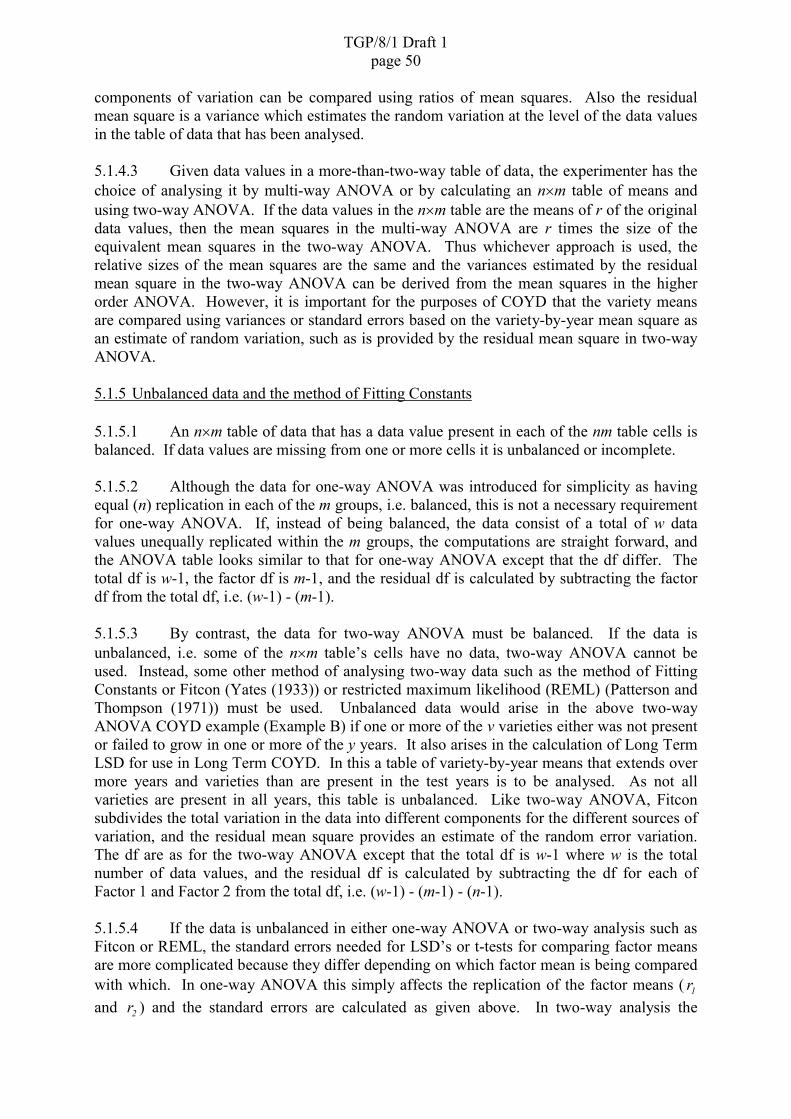
TGP/8/1 Draft 1page 50
components of variation can be compared using ratios of mean squares. Also the residualmean square is a variance which estimates the random variation at the level of the data valuesin the table of data that has been analysed.
5.1.4.3 Given data values in a more-than-two-way table of data, the experimenter has thechoice of analysing it by multi-way ANOVA or by calculating an n�m table of means andusing two-way ANOVA. If the data values in the n�m table are the means of r of the originaldata values, then the mean squares in the multi-way ANOVA are r times the size of theequivalent mean squares in the two-way ANOVA. Thus whichever approach is used, therelative sizes of the mean squares are the same and the variances estimated by the residualmean square in the two-way ANOVA can be derived from the mean squares in the higherorder ANOVA. However, it is important for the purposes of COYD that the variety meansare compared using variances or standard errors based on the variety-by-year mean square asan estimate of random variation, such as is provided by the residual mean square in two-wayANOVA.
5.1.5 Unbalanced data and the method of Fitting Constants
5.1.5.1 An n�m table of data that has a data value present in each of the nm table cells isbalanced. If data values are missing from one or more cells it is unbalanced or incomplete.
5.1.5.2 Although the data for one-way ANOVA was introduced for simplicity as havingequal (n) replication in each of the m groups, i.e. balanced, this is not a necessary requirementfor one-way ANOVA. If, instead of being balanced, the data consist of a total of w datavalues unequally replicated within the m groups, the computations are straight forward, andthe ANOVA table looks similar to that for one-way ANOVA except that the df differ. Thetotal df is w-1, the factor df is m-1, and the residual df is calculated by subtracting the factordf from the total df, i.e. (w-1) - (m-1).
5.1.5.3 By contrast, the data for two-way ANOVA must be balanced. If the data isunbalanced, i.e. some of the n�m table’s cells have no data, two-way ANOVA cannot beused. Instead, some other method of analysing two-way data such as the method of FittingConstants or Fitcon (Yates (1933)) or restricted maximum likelihood (REML) (Patterson andThompson (1971)) must be used. Unbalanced data would arise in the above two-wayANOVA COYD example (Example B) if one or more of the v varieties either was not presentor failed to grow in one or more of the y years. It also arises in the calculation of Long TermLSD for use in Long Term COYD. In this a table of variety-by-year means that extends overmore years and varieties than are present in the test years is to be analysed. As not allvarieties are present in all years, this table is unbalanced. Like two-way ANOVA, Fitconsubdivides the total variation in the data into different components for the different sources ofvariation, and the residual mean square provides an estimate of the random error variation.The df are as for the two-way ANOVA except that the total df is w-1 where w is the totalnumber of data values, and the residual df is calculated by subtracting the df for each ofFactor 1 and Factor 2 from the total df, i.e. (w-1) - (m-1) - (n-1).
5.1.5.4 If the data is unbalanced in either one-way ANOVA or two-way analysis such asFitcon or REML, the standard errors needed for LSD’s or t-tests for comparing factor meansare more complicated because they differ depending on which factor mean is being comparedwith which. In one-way ANOVA this simply affects the replication of the factor means ( 1rand 2r ) and the standard errors are calculated as given above. In two-way analysis the

TGP/8/1 Draft 1page 51
standard errors are further complicated because they depend on the pattern of missing valuesfor the two factor means being compared. However they are easily calculated by a computerprogram.
5.1.6 The paired t-test
The paired t-test is a special case of two-way ANOVA where the factor of interest has justtwo levels. Thus, it is used when there is an n�2 table of data corresponding to 2n data valuesclassified by two factors: Factor 1 with n levels and Factor 2, the factor of interest with 2levels. Examples of the paired t-test include:
(a) Each data value might be the plot yield from a trial with 2b plots laid out in b blocks (Factor 1) of 2 treatments (Factor 2);
(b) in DUS testing when a special test is set up to test distinctness between twovarieties using additional characteristics. A number of plants of each variety aresown in a trial. This is repeated in time with s independent sowings. In thisexample (Example E) the data values are the 2s means for the additionalcharacteristic, each based on a fixed number of established plants, from the ssowings (Factor 1) of the two varieties (Factor 2).
The analysis can be done in either of the two following ways:
5.1.6.1 The paired t-test using a one-sample t-test of differences
5.1.6.1.1 The difference in the two data values (one data value for each of the two levels ofFactor 2, the factor of interest) for each of the n levels of Factor 1 is obtained. This producesn differences denoted di, i=1,…,n. The mean difference and the variance of the differencesare calculated and used to produce the one sample t-statistic as follows:
)d(d
SEt �
where ��
�
n
iid
nd
1
1 is the mean difference, and � �n
d d2sSE � is the standard error of the mean
difference, and � ���
��
n
iid dd
n 1
22
1-1s is the variance of the differences, which is more easily
Example E: data from a special test with 2 varieties and s sowingsSowing 1 Sowing 2 Sowing 3 � Sowing s
Variety 1 - - - � -Variety 2 - - - � -
2s data valuesmean of all variety 1plants in sowing 2
mean of allvariety 2 plantsin sowing s

TGP/8/1 Draft 1page 52
computed as ��
�
�
��
�
�
���
�
� � ��
��
nddn
n
ii
n
iid
2
11
22
1-1s .
Providing the assumptions about the data discussed above are valid, this t-statistic can becompared with critical values from Student’s t-tables on n-1 df. The critical values should beone-tailed values if the sign of the mean difference is known a priori, and two-tailed valuesotherwise. The test is of whether the mean difference is significantly different from zero, i.e.whether Factor 2 has a significant effect.
If the absolute value of t is greater than or equal to the 100�p% critical value, the meandifference is declared to be significantly different from zero at the p% level. Otherwise, themean difference is declared to be not significantly different from zero at the p% level.
5.1.6.2 The paired t-test using two-way ANOVA
5.1.6.2.1 A standard two-way ANOVA of the n�2 table of data will provide an ANOVAtable with F-ratio’s of each of the Factor 1 and Factor 2 mean squares to the residual meansquare. Providing the assumptions about the data discussed above are valid, comparison ofthese F-ratios with F tables on the df of the numerator and the denominator mean squares willprovide “F-tests” to test whether Factors 1 and 2 have significant effects.
5.1.6.2.2 For Example E, the two-way ANOVA table is as follows:
Source of variationDegrees ofFreedom
Sum ofSquares
MeanSquare F-ratio
Sowing s - 1 - - -Variety 1 - - -Residual s - 1 - -
Total 2s - 1 -
5.1.6.2.3 The residual mean square from the two-way ANOVA can be used to estimate thevariance or standard errors of means calculated from the data. These can be used to calculatea two-sample t-statistic (or the equivalent LSD), which can be used to test the significance ofthe difference between the two factor means for Factor 2, i.e. test whether Factor 2 has asignificant effect
5.1.6.2.4 Whichever method of analysis is used, the significance of the test of the effect ofFactor 2 will be the same. In other words the significance of the t-test in the former methodwill be the same as the significance of the F-test of the Factor 2 effects and the significance ofthe t-test of the two Factor 2 means in the latter method.
5.1.6.2.5 A worked example of a paired t-test of the same type as Example E is given inAppendix A3.

TGP/8/1 Draft 1page 53
SECTION 6: EXAMINING DUS IN BULK SAMPLES
6.1 Introduction and abstract
In some crops samples are bulked before certain characteristics are examined. The term“bulk sampling” is used here for the process of merging some or all individual plants beforerecording a characteristic. There are different degrees of bulking ranging from: 1) mergingpairs of plants, 2) merging 3 or 4 up to all plants within a plot up to 3) merging all plantswithin a variety. The degree of bulking may play an important role in the efficiency of thetests. Bulking is usually only applied where the measurement of the characteristic is veryexpensive or very difficult to obtain for individual plants. Some examples are seed weight incereals and peas and beans, and erucic acid content in rapeseed. This section describes someof the consequences of bulk sampling. It is shown that the test of distinctness (using COYD,see Appendix A4 of section 5) may be expected to be relatively insensitive to the degree ofbulking, but that the efficiency of the tests for uniformity (using COYU, seedocument TGP/10, section 2) must be expected to decrease when the data are bulked. TheCOYU test for uniformity cannot be carried out if all plants within a plot are bulked.
6.2 Distinctness
6.2.1 In the COYD method for examining distinctness the basic values to be used in theanalyses are the annual variety means. As bulk sampling also gives at least one value for eachvariety per year, it will usually still be possible to use the COYD method for distinctnesspurposes for any degree of bulking, as long as at least one value is recorded for each varietyin each year and that the bulk samples are representative for the variety. However, someproblems may be foreseen: the assumption of data being normal distributed may be betterfulfilled when the mean of many individual measurements are analyzed instead of the mean offewer measurements or, in the extreme, just a single measurement.
6.2.2 The efficiency of the test of distinctness may be expected to be lower when based onbulked samples than when it is based on the mean of all individual plants in a year. The losswill be from almost zero upwards, depending on the importance of the different sources ofvariations. The variation which is relevant for the efficiency of variety comparisons isformulated in the following model.
2 2 2 2 2
2
2
where is the total variance of a characteristic used for comparing varieties
The total variance is regarded as being composed of four sources of variations:1: the year
total vy p i m
total
vy
� � � � �
�
�
� � � �
2
2
2
in which the variety is measured 2 : the plot in which the measurement was taken3: the plant on which the measurement was taken4 : the inaccuracy in the measurement process
p
i
m
�
�
�
6.2.3 In cases where the data are not bulked the variance of the difference between twovariety means, 2
diff� , becomes:

TGP/8/1 Draft 1page 54
2 2 2 22 2
whereis the number of years used in the COYD methodis the number of replicates in each trialis the number of plants in each plot
vy p i mdif a ab abc abc
abc
� � � �
�
� �� �� � � �� �
� ��
6.2.4 Assuming that each bulk sample has been composed in such a way that it represents anequal amount of material from all the individual plants which have been bulked into thatsample, the variance between two varieties based on k bulked samples (each of l plants)becomes:
2 2 2 22 2
whereis the number of bulk samples is the number of plants in each bulk sample
vy p i mdif a ab abkl abk
kl
� � � �
�
� �� �� � � �� �
� ��
6.2.5 Thus if all plants in each plot are divided in k groups of l plants each and an averagemeasurement is taken for each of the k groups, then only the last term in the expression for
2diff� has increased (as kl is equal to c). For many characteristics it is found that the variance
caused by the measurements process is small and hence the bulking of samples will only havea minor effect on the conclusions reached by the COYD method. Only if the variance causedby the measurement process is relatively large can bulking have a substantial effect on thedistinctness tests using COYD.
6.2.6 To illustrate the effect, the variances for comparing varieties were estimated (by the useof estimated variance components) for different degrees of bulking. The calculations werebased on the weight of 100 seeds of 145 pea varieties grown in Denmark during 1999 and2000. In this example, the contribution to the variance caused by the measurement processwas relatively very small, which means that bulking will have a low influence on the test fordistinctness. In a 3 year test with 30 plants in each of 2 blocks, the variance on a differencebetween two varieties was estimated to be 2.133 and 2.135, for no bulking and a single bulksample per plot, respectively. It should be noted that tests for uniformity are impossible ifonly 1 bulk per plot is used (see section 6.3).
6.2.7 For other variables the variance component due to the measurement process may berelatively more important. However, it is likely that in most practical cases this variancecomponent will be relatively small.
6.2.8 In some cases each bulk sample is not drawn from a specific set of plants (say, plant 1to 5 in bulk sample 1, plant 6 to 10 in bulk sample 2 etc.), but bulk samples are formed frommixed samples of all plants in a plot. This means that different bulk samples may containmaterial from the same plants. It must be expected that similar results apply here, although,in this situation, the effect of bulking may have an increased effect because there is noguarantee that all plants will be equally represented in the bulk samples.

TGP/8/1 Draft 1page 55
6.3 Uniformity
Bulking within plot
6.3.1 In COYU the test is based on the standard deviation between individual plants (withinplots) as a measurement of uniformity. The log of the standard deviations plus one areanalyzed in an over-years analysis; i.e. the values log( 1)vy vyZ s� � are used in the analyses.The variance on these Zvy values can be regarded as arising from two sources, a componentthat depends on the variety-by-year interaction and a component that depends on the numberof degree of freedom used for estimating the standard deviation, svy (the fewer degrees offreedom the more variable the standard deviation will be). This can be written (note that thesame symbols as used in the distinctness section will be used here with different meaning):
2 2
2
2
( )
where this variance can is regarded as being composed of two sources of variations:1: the year in which the variety is measured2 : the number of degrees of freedom using in estima
vy vy f
vy
f
Var Z � �
�
�
� �
22
ting
1 is approximately when then recorded variable is normally distributed and the 2 1
standard deviations do not vary too much. This last expression reduces to 0.5 / when 1.
vy
f
s
v�
�
�
� �
� �� ��� �
vy Here is the mean value of the s values and is the number of degrees of freedom used in
the estimation of .vys
� �
6.3.2 The variance caused by the year in which the variety is measured may be assumed to beindependent on whether the samples are bulked or not, whereas the variance caused by thenumber of degrees of freedom will be increase when bulked samples are used because a lowernumber of degrees of freedom is available.
6.3.3 The variance of a difference between a Zvy for a candidate variety and the mean of thereference varieties’ Zvy values may be written:
� �2 2 2 1 1
where is the number of year used in the test is the number of refference varieties
dif vy f a ar
ar
� � �� �
� � �� �� �
6.3.4 To illustrate the effect of bulking in the test for uniformity, an estimate was made usingthe same data as for the illustration in 8.6.2, paragraph 7. For a test using 50 referencevarieties in 3 years with 30 plants per variety in each of 2 plots per trial the variance forcomparing the Zvy value for a candidate variety and the mean of the reference varieties’ Zvywill be 0.0004 if no bulking is done. This can be compared to 0.0041, 0.0016 and 0.0007when 2, 4 and 10 bulk samples per plot were used. Thus, in this example, the effect ofbulking has a great influence on the test for uniformity. The variance increased,approximately by a factor of 10 when changing from individual plant records to just 2 bulk

TGP/8/1 Draft 1page 56
samples per plot. This means that the degree of non-uniformity must be much higher for it tobe detected when 2 bulk samples are used instead of individual plant records.
Bulking across plots
6.3.5 Bulking across plots means that part of the between plot (and block) variation will beincluded in the estimated standard deviation between bulked samples. If this variation isrelatively large it will tend to mask any differences in uniformity between varieties. Inaddition some noise may also be added because the ratio of material from the different plotsmay vary from bulk to bulk. Finally the assumptions for the present recommended method,COYU, may not be fulfilled in such cases. Therefore it is recommended to bulk only withinplots.
Taking just one bulk sample per plot
6.3.6 In general, if all plants in a plot are bulked such that only a single sample is availablefor each plot, it becomes impossible to calculate the within plot variability and in such casesno tests for uniformity can be performed. In rare cases, where non-uniformity may be judgedfrom values that can only be found in mixtures, non-uniformity may be detected even where asingle bulk sample for each plot is used. For example, in the characteristic “erucic acid” in oilseed rape, values between 2% and 45% can only arise because of a lack of uniformity.However this only applies in certain special cases and even here the non-uniformity may onlyshow up under certain circumstances.

TGP/8/1 Draft 1page 57
SECTION 7: THE GAIA METHODOLOGY
The GAIA method has been developed by experts from France to calculate a phenotypicdistance between two varieties. The principle is to compute a phenotypic distance between apair of varieties, which is a sum of distances for individual characteristics. For each species,this system must be calibrated to determine the weighting given to the difference in eachcharacteristic used and the threshold for the phenotypic distance used to eliminate varietiesfrom the growing trial.
7.1. Weighting of characteristics
7.1.1 Weighting is defined as the contribution in a given characteristic to the total distancebetween a pair of varieties. For each species, this system must be calibrated to determine theweight which can be given to each difference and to evaluate the reliability of eachcharacteristic in a given environment and for the genetic variability concerned. For thatreason the role of the crop expert is essential.
7.1.2 Weighting depends on the size of the difference and on the individualcharacteristic. The weightings are defined by crop experts on the basis of their expertise in thecrop and on a “try-and-check” learning process and stored in the GAIA database. Experts cangive zero weighting to small differences, thus, even if two varieties have different observedvalues in many characteristics, the overall distance might be zero. The same weighting isattributed to any pair of varieties whose absolute differences between observed values are thesame for a given characteristic.
7.1.3 The weighting should be simple and consistent. The following three rules aregiven:
(i) the distances for the characteristic should be integer values, i.e. 0, 1, 2, 3,etc. where 3 is considered to be about 3 times greater than 1;
(ii) if for a characteristic a given difference “expressed as an absolute value” isconsidered as a double distance for character a compared to character b, thedistance value for this difference should be double that in character a than it is incharacter b;
(iii) define the values by “try-and-check” (see Diagram 1.)
7.1.4 The following simple example shows the computation of the distance between twovarieties on the basis of a qualitative characteristic:
Example: taking the characteristic “Shape of ear”, observed on a 1 to 3 scale, the cropexperts have attributed weighting to differences which they consider significant:
Shape of ear:1 = conical2 = conico-cylindrical3 = cylindrical

TGP/8/1 Draft 1page 58
Comparison between difference in notes and weighting
Differentin notes
Weighting
conical (1) vs. conical (1) 0 0
conical (1) vs. conico-cylindrical (2) 1 2
conical (1) vs. cylindrical (3) 3 6
conico-cylindrical (2) vs. conico-cylindrical (2) 0 0
conico-cylindrical (2) vs. cylindrical (3) 1 2
cylindrical (3) vs. cylindrical (3) 0 0
When the crop experts compare a variety ‘i’ with conical ear (note 1) to a variety ‘j’with cylindrical ear (note 3), they attribute a weighting of 6 etc. The weightings aresummarized in the form of a weighting matrix:
Weighting matrix‘i’
Variety i
1 2 3
1 0 2 6
2 0 2
Var
iety
‘j’
3 0
When the crop experts compare a variety i with conical ear (note 1) to a variety jwith cylindrical ear (note 3), they attribute a weighting of 6.
7.2. Determining “Distinctness Plus”
The threshold for the phenotypic distance used to eliminate varieties from thegrowing trial is called “Distinctness Plus” and is determined by the crop expert at a levelwhich is higher than the difference needed to establish distinctness. This ensures that all pairsof varieties having a distance equal or greater than the threshold (Distinctness Plus) would bedistinct in the growing trial. The Distinctness Plus threshold must be based on experiencegained with the varieties of common knowledge and must minimize the possibility of notincluding in the growing trial a pair of varieties which should be further compared in the field.

TGP/8/1 Draft 1page 59
7.3. Computing GAIA phenotypic distance
7.3.1 The principle is to compute a phenotypic distance between two varieties, which isthe total distance between a pair of varieties as the result of the addition of the weightings ofall characteristics (see section 2 of this Annex). Thus, the GAIA phenotypic distance is:
��
�
ncharkk jiWjidist
,1
),(),(
where:),( jidist is the computed distance between variety i and variety j.
k is the kth characteristic, from the nchar characteristics selected for computation.Wk(i,j) is the weighting of characteristics k, which is a function of the differenceobserved between variety i and variety j for that characteristic k.OVki is the observed value on characteristic k for variety i.
� �kjkik OVOVfjiW ��),(
7.3.2 Varieties are compared in pairs in different combinations of pair-wise comparisons,e.g.:- compare two varieties,- compare a given variety to all varieties in the variety collection,- compare all candidate varieties to all the other candidate varieties and the
varieties in the variety collection,- compare all possible combinations.
7.4. The GAIA software
7.4.1 The GAIA software allows the computation of the phenotypic distance usingqualitative, quantitative or electrophoretic characteristics, which can be used alone or incombination. The user can decide on the type of data and the way it is used:
(i) select all the available characteristics, or different subsets of characteristics.
(ii) define different weighting values:
- experts can choose different values as the weighting/distance for acharacteristic (1, 2, 5, etc.);
- some crops have more characteristics than others;- the crop expert can use all available information, or a subset of characteristics
only.
(iii) the way the Distinctness Plus threshold is used:
- a low Distinctness Plus threshold, which helps to find the more difficult cases(to identify similar varieties- very often used by crop experts);
- intermediate Distinctness Plus threshold (different levels according to theneeds);

TGP/8/1 Draft 1page 60
- a large Distinctness Plus threshold when there is a need to have a comparisonwhich uses all the available characteristics;
- a Distinctness Plus threshold greater than the maximum distance possible on allcharacteristics to see all available raw data and the weightings for eachcharacteristic
7.4.2 The software provides a comprehensive report for each pair-wise comparison. Itcomputes an overall distance, but also provides all the individual absolute values and thedistance contribution of each characteristic (see section 6 of this Annex).
7.4.3 In order to minimize computation time, as soon as the threshold is achieved for acomparison between two given varieties, the software proceeds to the next pair of varieties.Remaining characteristics and their raw values will not be shown in the summary output, andwill not contribute to the distance.

TGP/8/1 Draft 1page 61
Select varieties andcharacteristics you
know very well
Define weighting forthe differences within
each characteristic
Compute and check ifresults are consistentwith your experience
Yes No
Reduce numberof varieties orcharacteristics
Select a larger set ofvarieties and/orcharacteristics
Define or update weightingfor some characteristics
Compute and check ifresults are consistentwith your experience
NoYes
Try to identify cases which puzzleyou, and to understand why. Is itcaused by: a new characteristic?;
the relative importance of 2characteristics? Are there a lot ofpuzzling cases, or only very few?
etc.
Exchange and show tocolleagues, breeders, etc.,that know the crop well
Validate weighting/ distances foreach characteristic, for use of the
software
Consider at time intervalswhether there is or not aneed to update the values
No need
Need
Diagram 1: “Try-and-check” process to define and revise the weightings for a crop

TGP/8/1 Draft 1page 62
7.4.4 Section 6 of this Annex provides a screen copy of a display tree which shows howthe expert can navigate and visualise the results of computations.
7.4.5 GAIA software has been developed with WINDEV-7.5. The general information(species, characteristics, weighting, etc.), the data collected on the varieties and the results ofcomputations are stored in an integrated database. Import and export facilities allow for otherinformation systems to be used in connection with the GAIA software. ODBC allows accessto the GAIA database and to other databases simultaneously.
7.4.6 For qualitative characteristics, 1 or 2 notes per variety can be used. In general, twonotes are present when there are two trial locations. For electrophoresis data, only onedescription can be entered per variety. For quantitative characteristics at least 2 values(different trials, repeats, etc.) are necessary and the user selects which to use in thecomputation.
7.4.7 GAIA is most suitable for self-pollinated and vegetatively propagated varieties, butcan also be used for other types of varieties.
7.5. Using the GAIA methodology
The GAIA methodology can be used:
(i) to eliminate from subsequent growing cycles all pairs of varieties reaching orsurpassing the GAIA distance threshold;
(ii) to focus on close varieties, having a GAIA distance lower than the threshold, forthe next growing cycle(s).
7.5.1 Using phenotypic distance in the first growing cycle
7.5.1.1 A crop that has a large variety collection and uses only quantitative characteristicson a 1 to 9 scale; the GAIA methodology allows the selection of varieties to be included inthe growing trial. This can be used to plan the first growing cycle trials as well as thesubsequent growing cycles.
7.5.1.2 In crops with relatively few candidates and a small variety collection, whichenables the crop expert to sow all candidates (e.g. an agricultural crop), and the appropriatereference varieties, in two or three successive growing cycles. The same varieties are sown ingrowing cycles 1, 2 and 3, in a randomized layout. The software will help to identify thepairs with a small distance, to enable the expert to focus his attention on these particular caseswhen visiting the field.
7.5.2 Using phenotypic distance after the first growing trial
7.5.2.1 After one growing cycle (e.g. in the examination of an ornamental crop), theabsolute data and distance computations are an objective way to confirm the opinion or thedecision of the expert. There might be cases where pairs of varieties have a small distance,but nevertheless the expert has clear evidence of distinctness. If more growing cycles arenecessary before a decision is taken, the software helps to identify on which cases the expertwill need to focus.

TGP/8/1 Draft 1page 63
7.5.2.2 In cases where there are many candidate and reference varieties and there is a widevariability in the species (e.g. a vegetable crop); on the one hand there are already obviousdifferences after only one cycle, but on the other hand some varieties are very similar. Inorder to be more efficient in their checks, the crop experts wish to grow “similar” varietiesclose to each other. The raw results and distances will help to select the “similar” varietiesand decide on the layout of the trial for the next growing cycle.
7.5.2.3 In crops in which there are many similar varieties, for which it is a commonpractice to make side-by-side comparisons, GAIA can be used to identify the similar varietiesafter the first cycle, in particular, when the number of varieties in a trial increases, making itless easy to identify all the problem situations. The software can help to “not miss” the lessobvious cases.
7.5.2.4 In vegetatively propagated ornamental varieties, the examination lasts for one ortwo growing cycles: after the first growing cycle, some reference varieties in the trial areobviously different from all candidates, and their inclusion in the second growing cycle is notnecessary. When the number of varieties is large, the raw data and distance(s) can help theexpert to detect reference varieties for which the second growing cycle is unnecessary.
7.6. Example with qualitative, electrophoretic and quantitative characteristics (Zea maysdata)
7.6.1 Introduction
7.6.1.1 The software can use qualitative, quantitative and/or electrophoretic data. Thesetypes of data can be used alone or in combination, as shown in Diagram 2.
Diagram 2: Data analysis scheme
Qualitative analysis
Gaia-distinctVarieties
Non Gaia-distinctVarieties
ElectrophoreticAnalysis
QuantitativeAnalysis
Gaia-distinctVarieties
Non Gaia-distinctVarieties Gaia-distinct
VarietiesNon Gaia-distinct
Varieties
QuantitativeAnalysis
Gaia-distinctVarieties
Non Gaia-distinctVarieties
Direct comparison in the fieldby the crop experts

TGP/8/1 Draft 1page 64
7.6.1.2 In this example, it is assumed that the crop expert has decided to use a DistinctnessPlus threshold Sdist of 10 (see section 2 of this Annex).
7.6.2 Qualitative Analysis
7.6.2.1 For each characteristic, weightings according to differences between levels ofexpression are pre-defined in a matrix of distances.
7.6.2.2 “Shape of ear”: observed on a 1 to 3 scale, the crop experts have attributedweightings greater than zero to differences which they consider significant:
1 = conical2 = conico-cylindrical3 = cylindrical
When the crop experts compare a variety ‘i’ with conical ear (note 1) to a variety ‘j’ withcylindrical ear (note 3), they attribute a weighting of 6.
7.6.2.3 “Length of husks”, observed on a 1 to 9 scale, the crop experts have defined thefollowing weighting matrix:
1 = very short2 = very short to short3 = short4 = short to medium5 = medium6 = medium to long7 = long8 = long to very long9 = very long
The weighting between a variety ‘i’ with very short husks (note 1) and a variety ‘j’ with shorthusks (note 3) is 0. Experts consider a difference of 3 notes is necessary in order to recognisea non-zero distance between two varieties. Even if the difference in notes is greater than 3,the experts do not increase the distance more than 2.
7.6.2.4 The reason for using a lower weighting for some characteristics compared to otherscan be that they are less “reliable” or “consistent” (e.g. more subject to the effect of theenvironment); and/or they are considered to indicate a lower distance between varieties.
Variety ‘i’ 1 2 31 0 2 62 0 2
Var
iety
‘j’
3 0
Variety ‘i’ 1 2 3 4 5 6 7 8 91 0 0 0 2 2 2 2 2 22 0 0 0 2 2 2 2 23 0 0 0 2 2 2 24 0 0 0 2 2 25 0 0 0 2 26 0 0 0 27 0 0 08 0 0
Var
iety
‘j’
9 0

TGP/8/1 Draft 1page 65
7.6.2.5 The matrix for a qualitative analysis for 5 characteristics for varieties A and B:
Earshape
Husklength
Type ofgrain
Numberof rowsof grain
Eardiameter
Notes for variety A (1 to 9 scale) 1 1 4 6 5
Notes for variety B (1 to 9 scale) 3 3 4 4 6
Difference observed 2 2 0 2 1
Weighting according to the crop expert 6 0 0 2 0 Dqual = 8
In this example Dqual = 8 < Sdist varieties A and B are declared “GAIA NON-distinct” and canbe passed on to electrophoretic analysis.
7.6.3 Electrophoretic analysis
7.6.3.1 The electrophoretic characteristic is a homozygous allele in the UPOV TestGuidelines (see Diagram 3). The software does not allow the use of heterozygous alleles.
2 genes
2 alleles 2 alleles
A characteristic observed as presence or absence
Idh1 4Idh1 6
IDHenzyme
Idh1(chromosome 8)
Idh2(chromosome 6)
Idh2 4Idh2 6
Diagram 3: The Isocitrate Deshydrogenase (IDH) enzyme has twogenes (Idh1 and Idh2) located on two different chromosomes. Eachof them has two alleles which are observed as 1 (presence) or0 (absence).
7.6.3.2 Electrophoretic characteristics are noted as 0 or 1 (absence or presence). Thedecision rule, used to give a weighting to two varieties, is the addition of the weightingnumber of differences observed and the weighting number of chromosomes related to thesedifferences (see example below):

TGP/8/1 Draft 1page 66
Chromosome 8 Chromosome 6
Idh1 4 Idh1 6 Idh2 4 Idh2 6
Variety A 0 1 1 0
Variety B 0 1 0 1
Difference 0 0 1 1
7.3.3 In this example, varieties A and B are described for 4 electrophoretic6.characteristics:
Idh1 4, Idh1 6, Idh2 4 and Idh2 6. The software looks at differences and gives the phenotypicdistance using the following computation:
Delec = 2x 0.25 + 1 x 1 = 1.5
7.6.3.4 This formula, which might be difficult to understand, was established by the cropexperts in collaboration with biochemical experts. Both the number of differences and thenumber of chromosomes on which differences are observed are used. Thus, less importance isattached to differences when these occur on the same chromosome, than when they occur ondifferent chromosomes.
7.6.3.5 After qualitative and electrophoretic analysis, the phenotypic distance betweenvarieties A and B is equal to:
D = Dqual + Delec = 8 + 1.5 = 9.5
The phenotypic distance is lower than Sdist, therefore varieties A and B are considered “GAIANON-distinct”.
7.6.3.6 It is not possible to establish distinctness solely on the basis of electrophoreticanalysis. It is necessary to have a minimal phenotypic distance in qualitative analysis in orderto take into account the electrophoresis results. This minimal phenotypic distance must alsobe defined by crop experts.
7.6.4 Quantitative Analysis
7.6.4.1 For each quantitative characteristic, the comparison of two varieties is made bylooking for consistent differences in at least two different experimental units. Experimentalunits are defined by the user depending on data present in the database. It can, for example,be the data from two geographic locations of the first growing cycle, or 2 or 3 replications inthe case of a single geographical location.
2 is the numberof differences
observed
0.25 is the weightingattributed by experts
to the number ofdifferences
1 is the number ofchromosome on
which differencesare observed
1 is the weightingassociated by
experts tochromosome.

TGP/8/1 Draft 1page 67
7.6.4.2 For a comparison to be made, the two varieties must be present in the sameexperimental units. The differences observed must be greater than one of the two thresholdvalues (or minimal distances), fixed by the crop experts.
- Dmin-inf is the lower value from which a weighting is attributed,
- Dmin-sup is the higher minimal distance. These values could be chosen arbitrarily orcalculated (15% and 20% of the mean for the trial, or LSD at 1% and 5%, etc.)
7.6.4.3 For each minimal distance a weighting is attributed:
- Dmin-inf a weighting Pmin is attributed;
- Dmin-sup a weighting Pmax is attributed;
- the observed difference is lower than Dmin-inf a zero weighting is associated.
7.6.4.4 Varieties A and B have been measured for characteristics “Width of blade” and“Length of plant” in two trials.
7.6.4.5 For each trial, and each characteristic, the crop experts have decided to define(Dmin-inf) and Dmin-sup by calculating respectively the 15% and 20% of the mean for the trial:
Width of blade Length of plantTrial 1 Trial 2 Trial 1 Trial 2
Dmin-inf = 15% of the mean 1.2 cm 1.4 cm 28 cm 24 cm
Dmin-sup = 20% of the mean 1.6 cm 1.9 cm 37 cm 32 cm
7.6.4.6 For each characteristic, the crop experts have attributed the following weighting:
A weighting Pmin = 3 is attributed when the difference is greater than Dmin-inf.
A weighting Pmax = 6 is attributed when the difference is greater than Dmin-sup.
Width of blade Length of plant
Trial 1 Trial 2 Trial 1 Trial 2
Variety A 9.9 cm 9.8 cm 176 cm 190 cm
Variety B 9.6 cm 8.7cm 140 cm 152 cm
Difference 0.3 cm 1.1 cm 36 cm 38 cm
Weighting according tothe crop expert 0 0 3 6 Dquan =?
7.6.4.7 In this example, for the characteristic “Width of blade”, the differences observedare lower than Dmin-inf, so no weighting is associated. On the other hand, for the characteristic“Length of plant” one difference is greater than the Dmin-inf value and the other is greater thanthe Dmin-sup value. These two differences are attributed different weightings.
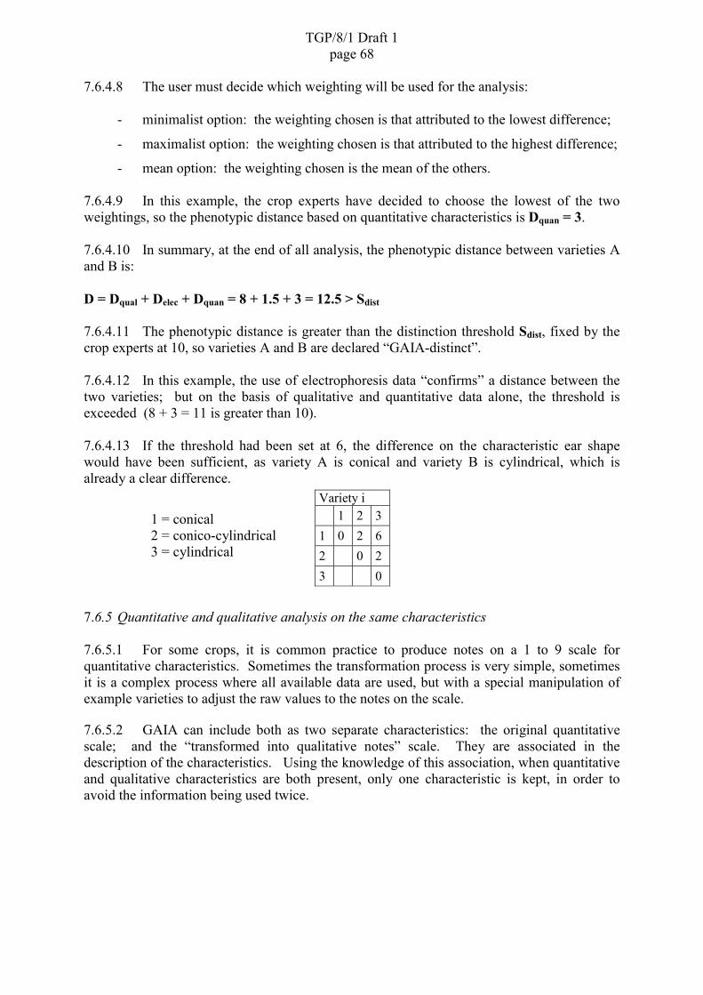
TGP/8/1 Draft 1page 68
7.6.4.8 The user must decide which weighting will be used for the analysis:
- minimalist option: the weighting chosen is that attributed to the lowest difference;
- maximalist option: the weighting chosen is that attributed to the highest difference;
- mean option: the weighting chosen is the mean of the others.
7.6.4.9 In this example, the crop experts have decided to choose the lowest of the twoweightings, so the phenotypic distance based on quantitative characteristics is Dquan = 3.
7.6.4.10 In summary, at the end of all analysis, the phenotypic distance between varieties Aand B is:
D = Dqual + Delec + Dquan = 8 + 1.5 + 3 = 12.5 > Sdist
7.6.4.11 The phenotypic distance is greater than the distinction threshold Sdist, fixed by thecrop experts at 10, so varieties A and B are declared “GAIA-distinct”.
7.6.4.12 In this example, the use of electrophoresis data “confirms” a distance between thetwo varieties; but on the basis of qualitative and quantitative data alone, the threshold isexceeded (8 + 3 = 11 is greater than 10).
7.6.4.13 If the threshold had been set at 6, the difference on the characteristic ear shapewould have been sufficient, as variety A is conical and variety B is cylindrical, which isalready a clear difference.
1 = conical2 = conico-cylindrical3 = cylindrical
7.6.5 Quantitative and qualitative analysis on the same characteristics
7.6.5.1 For some crops, it is common practice to produce notes on a 1 to 9 scale forquantitative characteristics. Sometimes the transformation process is very simple, sometimesit is a complex process where all available data are used, but with a special manipulation ofexample varieties to adjust the raw values to the notes on the scale.
7.6.5.2 GAIA can include both as two separate characteristics: the original quantitativescale; and the “transformed into qualitative notes” scale. They are associated in thedescription of the characteristics. Using the knowledge of this association, when quantitativeand qualitative characteristics are both present, only one characteristic is kept, in order toavoid the information being used twice.
Variety i 1 2 31 0 2 62 0 23 0

TGP/8/1 Draft 1page 69
7.7 GAIA screen copy.
The upper part shows 3 different computations which have been kept in the database.
The display tree on the left shows results for a [qualitative + electrophoresis at threshold of 6]computation.
Distinct cultivars [3] demonstrates that 3 varieties were found distinct from all others. Therewas a total of 52 (49 + 3) cultivars in the computation.
The display tree is used to navigate through all possible pairs.
The user can expand or reduce the branches of the tree according to his needs.
NON-distinct cultivars [49]. Forty-nine cultivars were found “not distinct from all others”with a threshold of 6.
The first variety, Variety 107, has only 3 close varieties, whereas the second, Variety 112, has9 close varieties, the third, Variety 113, 4 close varieties, etc.
The raw data for Variety 112 and Variety 26 are visible for the 6 qualitative characteristicsobserved on both varieties.
Variety 112 [1][9] indicates variety 112 is in the first year of examination [1]; and has9 close varieties according to the threshold of 6 [9].

TGP/8/1 Draft 1page 70
[dist=3.5]Variety 26 [2] indicates variety 26 has a GAIA distance of 3.5 from variety 112,which is in second year of examination.
The third column is the weighting according to the pre-defined matrices. The notes for bothvarieties are displayed for the two available locations (Std stands for “studied” which are thecandidate varieties).
In this screen copy the varieties have been numbered for sake of confidentiality, the cropexperts can name the varieties according to their need (lot or application number, name, etc.).
7.8 Final remark
The above example was described in order to explain how GAIA uses different types ofcharacteristics in a practical case. The efficiency of the use of GAIA depends on the species.

TGP/8/1 Draft 1page 71
REFERENCES
Dagnelie Pierre. (1981). Principes d’expérimentation
Dagnelie Pierre. (1998). Statistique théorique et appliquée volume 2 inférence statistique àune et deux dimensions. Bibliothèque des universités Statistique
Digby, P.G.N. (1979). Modified joint regression analysis for incomplete variety xenvironment data. J. Agric. Sci. Camb. 93, 81-86.
Kala, R. (2002). Statystyka dla przyrodnikow, Agric. Univ. of Poznan
Mead, R., Curnow, R. N. and Hasted, R. M. (1993). Statistical Methods in Agriculture andExperimental Biology. Chapman & Hall, London.
Patterson, H. D. and Thompson, R. (1971). Recovery of interblock information when blocksizes are unequal. Biometrika, 58, 545-554.
Patterson, H.D. & Weatherup, S.T.C. (1984). Statistical criteria for distinctness betweenvarieties of herbage crops. J. Agric. Sci. Camb. 102, 59-68.
Sokal, R. R. and Rohlf, F. J. (1995). Biometry, W. H. Freeman Company
Talbot, M. (1990). Statistical aspects of minimum distances between varieties. UPOV TWCPaper TWC/VIII/9, UPOV, Geneva.
Yates, F. (1933). The principles of orthogonality and confounding in replicated experiments.Journal of Agricultural Science, Cambridge, 23, 108-45.

TGP/8/1 Draft 1page 72
APPENDICES
APPENDIX A1
Example of two-way ANOVA (same type as Example A)
1. A trial with four blocks of five varieties of Kale was sown with 15 plants per plot. Thedata below are the plot means over all the plants in a plot for the “petiole length in mm”characteristic.
BlockVariety I II III IV
J 361 375 361 399K 388 383 376 401L 356 386 365 382M 383 373 385 405N 386 385 389 413
2. Two-way ANOVA of the data produces the following table:
Source of variationDegrees ofFreedom
Sum ofSquares
MeanSquare F-ratio
Block 3 2116.00 705.33 9.95Variety 4 1316.30 329.08 4.64Residual 12 850.50 70.88
Total 19 4282.80
3. From F-tables the 5%, 1% and 0.1% critical values on 4 and 12 df are 3.259, 5.412 and9.633 respectively. Comparison of the Variety F-ratio with these shows that there is asignificant variety effect at the 5% level (P<0.05). The residual mean square or variety-by-block mean square is an estimate of the random variability of the 20 values in the above datatable. It may be used to estimate the variance or standard errors of means calculated from thedata.
4. The variety means are the means of 4 data values and are as follows:
Variety Mean
J 374.0K 387.0L 372.2M 386.5N 393.2
5. Their standard error, )SE(x , is estimated by
2144
70.88)SE( .r
RMSx ���

TGP/8/1 Draft 1page 73
6. The standard error of the difference in two means, ( )-SE( 21 xx ), is estimated by
95541
4188011)-SE( ..7
rrRMSxx
2121 ��
�
���
�����
�
����
���
7. The significance of the difference between pairs of variety means can be tested bycomparing the absolute difference between pairs of means with, for example, the 5% LSD,where
5% LSD = 97129551792SE ...)xx(t 21 �����
and t is the 5% two-tailed critical value from Students' t-tables on 12 df. Thus varieties J andK are significantly different at the 5% level, whereas varieties J and L and varieties M and Nare not significantly different at the 5% level etc.
Example of two-way ANOVA (same type as Example B)
8. This example illustrates the calculation of the COYD criterion. The data are thevariety-by-year means for 11 varieties of italian ryegrass in three years for the “plant width incm at ear emergence” characteristic.
Variety Year 1 Year 2 Year 3
L 60.66 61.47 55.18N 58.91 62.28 55.66O 54.46 56.68 51.32P 57.69 54.75 54.94Q 56.57 57.62 51.46R 51.33 53.40 49.18S 58.59 59.08 51.67T 63.47 58.94 54.97V 66.14 65.49 60.15W 62.63 63.90 58.84AC 60.36 58.42 58.51
9. Two-way ANOVA of the data produces the following table:
Source of variationDegrees ofFreedom
Sum ofSquares
MeanSquare F-ratio
Year 2 148.821 74.4106 26.843Variety 10 383.679 38.3679 13.841Residual 20 55.443 2.7721
Total 31 587.944
10. From F-tables the 5%, 1% and 0.1% critical values on 10 and 20 df are 2.348, 3.368 and5.075 respectively. Comparison of the Variety F-ratio with these shows that there is a veryhighly significant variety effect at the 0.1% level (P<0.001). The residual mean square or

TGP/8/1 Draft 1page 74
variety-by-year mean square is an estimate of the random variability of the 33 values in theabove data table. It may be used to estimate the variance or standard errors of meanscalculated from the data.
11. The variety means are the means of 3 data values and are as follows:
Variety Mean
L 59.103N 58.950O 54.153P 55.793Q 55.217R 51.303S 56.447T 59.127V 63.927W 61.790AC 59.097
12. Their standard error, )SE(x , is estimated by
9613.03
2.7721)SE( ���
rRMSx
13. The standard error of the difference in two means, ( )-SE( 21 xx ), is estimated by
3594.131
317721.11)-SE( ��
�
���
�����
�
����
��� 2
rrRMSxx
2121
14. The significance of the difference between pairs of variety means can be tested bycomparing the absolute difference between pairs of means with the 1% LSD where
1% LSD = 868.33594.1584.2)(SE ����� 21 xxt
and t is the 1% two-tailed critical value from Student’s t-tables on 20 df. Thus varieties Land N are not significantly different at the 1% level, whereas varieties L and O and varieties Land Q are significantly different at the 1% level etc.
15. For more information on the COYD criterion see document TGP/9.7.

TGP/8/1 Draft 1page 75
APPENDIX A2
Example of one-way ANOVA (same type as Example C)
1. The data below are the plot yields in Kg from a glasshouse experiment consisting of 18pots (plots) of potato plants to which 3 replicates of each of six fungicide treatments wereallocated at random.
Replicate Treat’1
Treat’2
Treat’3
Treat’4
Treat’5
Treat’6
1 1.07 0.23 1.07 0.66 1.07 0.912 0.74 0.54 0.63 0.85 1.31 0.943 0.89 0.57 1.08 0.78 1.50 0.66
2. One-way ANOVA of the data produces the following table:-
Source of variationDegrees ofFreedom
Sum ofSquares
MeanSquare F-ratio
Treatments 5 1.1236 0.2247 6.48Residual 12 0.4161 0.0347
Total 17 1.5398
3. From F-tables the 5%, 1% and 0.1% critical values on 5 and 12 df are 3.106, 5.064 and8.892 respectively. Comparison of the Treatment F-ratio with these shows that there is ahighly significant treatment effect at the 1% level (P<0.01) on the plot yield. The residualmean square is an estimate of the random variability of the 18 values in the above data table.It may be used to estimate the variance or standard errors of means calculated from the data.
4. The treatment means are the means of 3 data values and are as follows:-
Treatment Mean
1 0.9002 0.4473 0.9274 0.7635 1.2936 0.837
5. Their standard error, )SE(x , is estimated by
107503
0.0347)SE( .r
RMSx ���
6. The standard error of the difference in two means, ( )-SE( 21 xx ), is estimated by

TGP/8/1 Draft 1page 76
1521031
310347011)-SE( ..
rrRMSxx
2121 ��
�
���
�����
�
����
���
7. The significance of the difference between pairs of treatment means can be tested bycomparing the absolute difference between pairs of means with, for example, the 5% LSD,where
5% LSD = 33130152101792SE ...)xx(t 21 �����
and t is the 5% two-tailed critical value from Student’s t-tables on 12 df. Thus treatments 1and 2 and treatments 1 and 5 are significantly different at the 5% level, whereas treatments 1and 3 are not significantly different at the 5% level etc.
Example of one-way ANOVA (same type as Example D)
8. This example illustrates a stage in the calculation of the COYU criterion. The data arethe variety-by-year adjusted log(SD+1) of the “days to ear emergence” characteristic for 11reference varieties of perennial ryegrass in three years. The data have been adjusted for anyrelationships between log(SD+1) and mean values for the characteristic. The data are asfollows:
Variety Year 1 Year 2 Year 3
R1 2.36 2.13 2.30R2 2.32 2.00 2.00R3 2.42 2.10 1.95R4 2.43 1.96 2.06R5 2.52 2.14 1.96R6 2.36 1.84 2.16R7 2.43 2.19 1.80R8 2.44 1.70 1.91R9 2.52 2.16 2.24R10 2.33 2.23 2.09R11 2.28 1.78 1.96
9. One-way ANOVA of the data produces the following table:-
Source of variationDegrees ofFreedom
Sum ofSquares
MeanSquare F-ratio
Year 2 1.011 0.5053 25.06Residual 30 0.605 0.0202
Total 32 1.616
10. From F-tables the 5%, 1% and 0.1% critical values on 2 and 30 df are 3.316, 5.390 and8.773 respectively. Comparison of the Year F-ratio with these shows that there is a veryhighly significant year effect at the 0.1% level (P<0.001) on uniformity. However, this F-testis of minor importance in calculating the COYU criterion. Of real importance is the overallmean adjusted log(SD+1) for all the reference varieties, and the residual mean square. Theresidual mean square provides an estimate of the random variability of the 33 values in the

TGP/8/1 Draft 1page 77
above data table, i.e. the variation between reference varieties within years. It may be used toestimate the variance or standard errors of means calculated from the data. In particular, itallows the overall mean of the reference varieties to be compared with a candidate variety’smean adjusted log(SD+1).
11. The overall mean adjusted log(SD+1) is 2.154. It is the mean of the reference varieties’33 data values. Its standard error, )SE(x , is estimated by
0247.033
0.0202)SE( ���
rRMSx
12. If 1x represents the overall mean adjusted log(SD+1) and 2x a candidate variety’s meanadjusted log(SD+1) which is the mean of the equivalent of 3 data values, then the standarderror of the difference in the two means, ( )-SE( 21 xx ), is estimated by
0857.031
3310202.011)-SE( ��
�
���
�����
�
����
���
2121 rr
RMSxx
13. The significance of the difference between 1x , the overall mean adjusted log(SD+1) and
2x , a candidate variety’s mean adjusted log(SD+1) can be tested by comparing
1221 xxxx ��� with 2672.00857.0118.3)(SE ����� 21 xxt
Where t is the 0.2% one-tailed critical value (one-tailed because the candidate’s mean is onlyrejected if it is larger than the overall mean) from Student’s t-tables on 30 df. This isequivalent to comparing
2x with 4212.22672.0 �� 1x
14. Thus if a candidate variety has a mean adjusted log(SD+1) greater than or equal to2.42*, this mean is significantly greater than the mean of the reference varieties at the 0.2%level, and hence the candidate variety is considered to be significantly non-uniform comparedto the reference varieties. If the candidate variety’s mean adjusted log(SD+1) is less than2.42*, the mean will be considered to be not significantly different from the mean of thereference varieties at the 0.2% level, and hence the candidate variety not significantlydifferent from the reference varieties in uniformity.
* The above is based on the conventional use of the two sample t-test. However, in order togive the benefit of the doubt to the breeder, in the practical application of COYU the acceptedprocedure is to reject a variety as non-uniform if its mean adjusted log(SD+1) is greater thanthe uniformity criterion, and accept it as uniform if its mean adjusted log(SD+1) is less thanor equal to the uniformity criterion.
15. For more information on the COYU criterion see document TGP/10.3.1.

TGP/8/1 Draft 1page 78
APPENDIX A3
Example of a paired t-test (same type as Example E)
1. A special test was set up in order to test distinctness between two varieties of perennialryegrass using the additional characteristic “Seedling width of vegetative leaf”. Thirty plantsof each variety were sown at each independent sowing in a glasshouse, and when the plantswere established, the “Seedling width of vegetative leaf” was observed in mm on each plant,and the mean for each variety calculated. There were 6 independent sowings and the databelow are the 12 means: one for each variety for each sowing.
SowingVariety I II III IV V VI
J 6.9 7.9 5.2 5.8 6.5 4.8N 5.9 6.7 3.8 5.3 3.6 3.6
2. The data will be analysed using each of the described methods.
The paired t-test analysis using a one-sample t-test of differences
3. Subtracting the variety N data value from the variety J data value for each sowing givesthe following differences:-
SowingI II III IV V VI
Difference (di) 1.0 1.2 1.4 0.5 2.9 1.2
4. The mean difference d , the variance of the differences 2sd , and the standard error of themean difference � �dSE are calculated from the differences as follows:-
��
�
n
iid
nd
1
1� � 37128
6121412101
61
61 6
1.........d
ii ��������� �
�
��
�
�
��
�
�
���
�
� � ��
��
nddn
n
ii
n
iid
2
11
22
1-1s
��
�
�
��
�
�
���
�
� � ��
��
61-6
126
1
6
1
2
ii
ii dd
� � ��
���
���������� �
�
6214121012141210151 2
6
1
2222 ..............i
� �� � 6587062851451 2 ... ���
� �n
d d2sSE � 33130
665870 ..
��
5. These are used to calculate the one sample t-statistic as follows:-
)d(d
SEt � 124
331301.37 ..
��

TGP/8/1 Draft 1page 79
6. From Student’s t-tables the 5%, 1% and 0.1% two-tailed critical values on 5 df are2.571, 4.032 and 6.869 respectively. Comparison of the t-statistic with these shows that themean difference is highly significantly different from zero at the 1% level (P<0.01), i.e.Variety has a highly significant effect. From the sign of the mean difference it is apparentthat variety J has a greater “Seedling width of vegetative leaf” than variety N.
The paired t-test analysis using two-way ANOVA
7. Two-way ANOVA of the data produces the following table:-
Source of variationDegrees ofFreedom
Sum ofSquares
MeanSquare F-ratio
Sowing 5 13.8900 2.7780 8.44Variety 1 5.6033 5.6033 17.01Residual 5 1.6467 0.3293
Total 11 21.1400
8. From F-tables the 5%, 1% and 0.1% critical values on 1 and 5 df are 6.608, 16.26 and47.18 respectively. Comparison of the Variety F-ratio with these shows that there is a highlysignificant Variety effect at the 1% level (P<0.01). The residual mean square or variety-by-sowing mean square is an estimate of the random variability of the 12 values in the above datatable. It may be used to estimate the variance or standard errors of means calculated from thedata.
9. The variety means are the means of 6 data values and are as follows:-
Variety Mean
J 6.18N 4.82
10. Their standard error, )SE(x , is estimated by
234306
0.3293)SE( .r
RMSx ���
11. The standard error of the difference in two means, ( )-SE( 21 xx ), is estimated by
3313061
613293011)-SE( ..
rrRMSxx
2121 ��
�
���
�����
�
����
���
12. The significance of the difference between the two variety means can be tested bycalculating the two sample t-statistic:
)xx(xx
21
21
�
�
�
SEt 124
0.33134.826.18 .�
�
�

TGP/8/1 Draft 1page 80
From Student’s t-tables on 5 df, the 5%, 1% and 0.1% two-tailed critical values are 2.571,4.032 and 6.869 respectively. Comparison of the t-statistic with these shows that thedifference in the variety means is highly significant at the 1% level (P<0.01), i.e. variety J hasa greater ‘Seedling width of vegetative leaf’ than variety N.

TGP/8/1 Draft 1page 81
APPENDIX A4
5.2 The Combined Over-Years Distinctness Criterion (COYD)
5.2.1 Summary
5.2.1.1 To distinguish varieties on the basis of a quantitative characteristic we need toestablish a minimum distance between varieties such that, when the distance calculatedbetween a pair of varieties is greater than this minimum distance, they may be considered as“distinct” in respect of that characteristic. There are several possible ways of establishingminimum distances from Distinctness, Uniformity and Stability (DUS) trials data. Here isdescribed what is known as the Combined-Over-Years Distinctness (COYD) method.
5.2.1.2 The COYD method involves:
– for each characteristic, taking the variety means from the two or three years oftrials for candidates and established varieties and producing over-year means forthe varieties;
– calculate a least significant difference (LSD), based on variety-by-years variation,for comparing variety means.
– if the over-years mean difference between two varieties is greater than or equal tothe LSD then the varieties are said to be distinct in respect of that characteristic.
5.2.1.3 The main advantages of the COYD method are:
– it combines information from several seasons into a single criterion (the “COYDcriterion”) in a simple and straightforward way;
– it ensures that judgements about distinctness will be reproducible in other seasons;
in other words, the same genetic material should give similar results, withinreasonable limits, from season-to-season;
– the risks of making a wrong judgement about distinctness are constant for all
characteristics.
5.2.2 Introduction
5.2.2.1 In order to decide if two varieties are distinct in respect of a measuredcharacteristic, a criterion is needed which will determine whether the differences found inDUS trials are clear and sufficiently consistent. The Combined-Over-Years Distinctness(COYD) method provides such a criterion.
5.2.2.2 This paper describes:
– the principles underlying the COYD method;
– UPOV recommendations on the application of COYD to individual species;

TGP/8/1 Draft 1page 82
– details of ways in which the procedure can be adapted to deal with specialcircumstances. This includes when there are small numbers of varieties in trial;
– the computer software which is available to apply the procedure.
5.2.3 The COYD Method
5.2.3.1 The COYD method aims to establish for each characteristic a minimum difference,or distance, which, if achieved by two varieties in trials over a period of two or three years,would indicate that those varieties are distinct with a specified degree of confidence.
5.2.3.2 The method uses variation in variety expression of a characteristic from year-to-year to establish the minimum distance. Thus, characteristics which show consistency invariety ranking between years will have smaller minimum distances than those with markedchanges in ranking.
5.2.3.3 Calculation of the COYD criterion involves analysing the variety-by-year table ofmeans for each characteristic to get an estimate of the varieties-by-years variation, which isused in the next step: to calculate an LSD. Usually data for all candidate and establishedvarieties which appeared in trials over the two or three test years are included in the table, theanalysis is by analysis of variance (see TGP/8.5 for details), the varieties-by-years meansquare is used as the estimate of the varieties-by-years variation, and the resulting LSD isknown as the COYD LSD. However, where there are small numbers of varieties in trial, theapproach is different.
5.2.3.4 Where there are small numbers of varieties in trial, the table used to calculate of theCOYD criterion is expanded with means from other varieties and earlier years, a differentmethod of analysis is used to get a varieties-by-years mean square to estimate the varieties-by-years variation, and the resulting LSD is known as the Long-Term LSD. This is discussedlater.
5.2.3.5 Equation [1]LSDp = tp x �2 x SE( x )
where )(SE x is the standard error of a variety’s over-year mean calculated as:
years test ofnumber squaremean years-by-varietiesSE �)x(
and tp is the value in Student’s t table appropriate for a two-tailed test with probability p
and with degrees of freedom associated with the variety-by-years mean square.The probability level p that is appropriate for individual species is discussedunder UPOV RECOMMENDATIONS ON COYD below.
5.2.3.6 An example of the application of COYD to a small data set is given in Figure 1.Statistical details of the method are in Annex IV and in document TGP/8.5, “StatisticalMethods for DUS Examination.” Further information about the COYD criterion can be foundin Patterson and Weatherup (1984).

TGP/8/1 Draft 1page 83
5.3 UPOV Recommendations on COYD
5.3.1 COYD is recommended for use in assessing the distinctness of varieties where:
– the characteristic is quantitative; – there are some differences between plants (or plots) of a variety. – observations are made on a plant (or plot) basis over two or more years;
5.3.2 A pair of varieties is considered to be distinct if their over-years means differ by atleast the COYD LSD in one or more characteristics.
5.3.3 The UPOV recommended probability level p for the tp value used to calculate theCOYD LSD differs depending on the crop and for some crops depends on whether the test isover two or three years. The testing schemes that usually arise in distinctness testing aredescribed in Annex VI.
5.4 Adapting COYD to special circumstances
5.4.1 Differences between years in the range of expression of a characteristic.Occasionally, marked differences between years in the range of expression of a characteristiccan occur. For example, in a late spring, the heading dates of grass varieties can converge.To take account of this effect it is possible to fit extra terms, one for each year, in the analysisof variance. Each term represents the linear regression of the observations for the year againstthe variety means over all years. The method is known as modified joint regression analysis(MJRA) and is recommended in situations where there is a statistically significant (p � 1%)contribution from the regression terms in the analysis of variance. Statistical details, and acomputer program to implement the procedure, are described in the appendices.
5.5 Small numbers of varieties in trials: Long-Term COYD
5.5.1 It is recommended that there should be at least 20 degrees of freedom for thevarieties-by-years mean square in the COYD analysis of variance. This is in order to ensurethat the varieties-by-years mean square is based on sufficient data to be a reliable estimate ofthe varieties-by-years variation for the LSD. Twenty degrees of freedom corresponds to11 varieties common in three years of trials, or 21 varieties common in two years. Trials withfewer varieties in common over years are considered to have small numbers of varieties intrial.
5.5.2 In such trials the variety-by-year tables of means can be expanded to include meansfor earlier years, and if necessary, other established varieties. As not all varieties are presentin all years, the resulting tables of variety-by-year means are not balanced. Consequently,each table is analysed by the least squares method of fitted constants (FITCON) or by REML,which produces an alternative varieties-by-years mean square as a long-term estimate ofvariety-by-years variation. This estimate has more degrees of freedom as it is based on moreyears and varieties.
� � � � 1years No. varietiesNo.year table-by-variety expandedin valuesNo.freedomofdegrees ������
���

TGP/8/1 Draft 1page 84
5.5.3 The alternative varieties-by-years mean square is used in equation [1] above tocalculate an LSD. This LSD is known as a “Long-Term LSD” to distinguish it from COYDLSD based on just the test years and varieties. The Long-Term LSD is used in the same wayas the COYD LSD is used to assess the distinctness of varieties by comparing their over-year(the test years) means. The act of comparing the means of varieties using a “Long-TermLSD” is known as “Long-Term COYD”.
5.5.4 Long-Term COYD should only be applied to those characteristics lacking therecommended minimum degrees of freedom. However, when there is evidence that acharacteristic’s LSD fluctuates markedly across years, it may be necessary to base the LSDfor that characteristic on the current two or three-years of data, even though it has few degreesof freedom.
5.5.5 Figure 2 gives an example of the application of Long-Term COYD to the italianryegrass characteristic "Growth habit in spring" (UPOV Char 6). A flow diagram of thestages and DUST modules used to produce Long-Term LSD’s and perform Long-TermCOYD is given in Figure B2 in Annex V.
5.6 Marked year-to-year changes in an individual variety’s characteristic
Occasionally, a pair of varieties may be declared distinct on the basis of a t-testwhich is significant solely due to a very large difference between the varieties in a single year.To monitor such situations a check statistic is calculated, called F3, which is the variety-byyears mean square for the particular variety pair expressed as a ratio of the overall variety-by-years mean square. This statistic should be compared with F-distribution tables with 1 and g,or 2 and g, degrees of freedom, for tests with two or three years of data respectively where gis the degrees of freedom for the variety-by-years mean square. If the calculated F3 valueexceeds the tabulated F value at the 1% level then an explanation for the unusual result shouldbe sought before making a decision on distinctness.
5.7 Implementing COYD
The COYD method can be applied using the DUST package for the statisticalanalysis of DUS data, which is available from Dr. Sally Watson, Biometrics Division,Department of Agriculture for Northern Ireland (DANI), Newforge Lane, Belfast BT9 5PX,United Kingdom. Sample outputs are given in Annex V.

TGP/8/1 Draft 1page 85
Figure 1: Illustrating the calculation of the COYD criterion
Characteristic: Days to ear emergence in perennial ryegrass varieties
YearsOverYear
Varieties 1 2 3 Means
Difference(Varietiescompared
to C2)Reference MeansR1 38 41 35 38 35 DR2 63 68 61 64 9 DR3 69 71 64 68 5 DR4 71 75 67 71 2R5 69 78 69 72 1R6 74 77 71 74 -1R7 76 79 70 75 -2R8 75 80 73 76 -3R9 78 81 75 78 -5 DR10 79 80 75 78 -5 DR11 76 85 79 80 -7 DCandidateC1 52 56 48 52 21 DC2 72 79 68 73 0 -C3 85 88 85 86 -13 D
ANALYSIS OF VARIANCE
Source df Mean squareYears 2 174.93Variety 13 452.59Variety-by-years 26 2.54
LSDp = tp * 2 * SE( )X
LSD0.01 = 2.779 * 1.414 * (2.54/3) = 3.6
Where tp is taken from Student’s t table with p = 0.01 (two-tailed) and 26 degrees offreedom.
To assess the distinctness of a candidate, the difference in the means between the candidateand all other varieties is computed. In practice a column of differences is calculated foreach candidate. In this case, varieties with mean differences greater than, or equal to, 3.6are regarded as distinct (marked D above).

TGP/8/1 Draft 1page 86
Figure 2: Illustrating the application of Long-Term COYD
Characteristic: Growth habit in spring in italian ryegrass varieties
YearsVarieties 1 2 3* 4* 5*
Mean overtest years
Difference(Varieties
compared to C2)Reference MeansR1 43 42 41 44R2 39 45R3 43 38 41 45 40 42 6 DR4 44 40 42 48 44 44.7 3.3 DR5 46 43 48 49 45 47.3 0.7R6 51 48 52 53 51 52 -4 DCandidateC1 43 45 44 44 4 DC2 49 50 45 48 0C3 48 53 47 49.3 -1.3
* indicates a test year
The aim is to assess the distinctness of the candidate varieties C1, C2 & C3 grown in thetest years 3, 4 & 5.
The trial has a small number of varieties in trial because there are just seven varieties incommon over the test years 3, 4 & 5 (data marked by a black border).
FITCON analysis of the variety-by-years table of means expanded to nine varieties infive years gives: varieties-by-years mean square = 1.924, on 22 degrees of freedom
Long-term LSDp = t p * 2 * SE( )X
Long-term LSD0.01 = 2.819 * 1.414 * (1.924/3) = 3.19
Where tp is taken from Student’s t table with p = 0.01 (two-tailed) and 22 degrees offreedom
To assess the distinctness of a candidate, the difference in the means between thecandidate and all other varieties is computed. In practice a column of differences iscalculated for each candidate. In the case of variety C2, varieties with mean differencesgreater than, or equal to 3.19 are regarded as distinct (marked D above).
[End of document]