introduction to dna cell cycle analysis

Basics of DNA Cell Cycle Analysiswww.phoenixflow.com

The Biological Cell Cycle .........................2

DNA Analysis and theFlow Cytometric Cell Cycle ....................3

Diploid and Aneuploid DNA Contents......5

Cell Cycle Analysis ofDNA Content Histograms.........................6

Fitting of Background “Debris” andEffects of Nucleus Sectioning ..................9

Fitting and Correction for the Effectsof Cellular or Nuclear Aggregation.........16

Quantitation of Background, AggregatesAnd Debris.....................................................31

Analysis of Apoptosis .............................31

Beyond Single Parameter Analysis:DNA vs. Immunofluorescence................32

INTRODUCTION TO CELL CYCLE ANALYSIS

Written byDr. Peter Rabinovitch, M.D., Ph.D.

Published byPhoenix Flow Systems, Inc.

6790 Top Gun St. #1San Diego, CA. USA 92121

858 453-5095fax 858 453-2117


This chapter is organized into progressively more advanced sections. Feel freeto skip ahead to the level appropriate for your background.

THE BIOLOGICAL CELL CYCLE

Reproduction of cells requires cell division, with production of two daughtercells. The most obvious cellular structure that requires duplication anddivision into daughter cells is the cell nucleus - the repository of the cell'sgenetic material, DNA. With few exceptions each cell in an organismcontains the same amount of DNA and the same complement ofchromosomes. Thus, cells must duplicate their allotment of DNA prior todivision so that each daughter will receive the same DNA content as theparent.

The cycle of increase in components (growth) and division, followed bygrowth and division of these daughter cells, etc., is called the cell cycle. Thetwo most obvious features of the cell cycle are the synthesis and duplicationof nuclear DNA before division, and the process of cellular division itself -mitosis. These two components of the cell cycle are usually indicated inshorthand as the “S phase” and “mitosis” or “M”.

When the S phase and M phase of the cell cycle were originally described, itwas observed that there was a temporal delay or gap between mitosis andthe onset of DNA synthesis, and another gap between the completion of DNAsynthesis and the onset of mitosis. These gaps were termed G1 and G2,respectively. The cycle of G1 → S → G2 → M → G1, etc., is shownschematically in Figure 2.1.

Figure 2.1. A schematic of the cell cycle, showing flowcytometric components of each phase


When not in the process of preparing for cell division, (most of the cells inour body are not), cells remain in the G1 portion of the cell cycle. The G1phase is thus numerically the most predominant phase of the cell cycle andshows up as the largest peak. A subset of G1 cells which are very quiescentand have little of the cellular functions needed to enter the cell cycle aresometimes referred to as G0 cells.

Some of the cellular processes, which take place in the G1 and G2 phases ofthe cell cycle, are now known. The G1 phase is a synthetic growth phase formany RNA and protein molecules that will be needed for DNA synthesis andcell growth before division. The G2 phase is a time for repair of any DNAdamage which has occurred during the preceding cell cycle phases, and forthe reorganization of the DNA structure which must take place before theDNA can be divided equally between daughters during Mitosis.

The length of these phases may vary between different cell types that areactively in the process of cell division. Typical time spans in which the cell isengaged in each of the phases of the cell cycle are 12 hours for G1, 6 hoursfor S phase, 4 hours for G2, and 0.5 hour for Mitosis.

DNA ANALYSIS AND THE

FLOW CYTOMETRIC CELL CYCLE

One of the earliest applications of flow cytometry was the measurement ofDNA content in cells; the first rapid identification of phases of the cell cycleother than mitosis. This analysis is based on the ability to stain the cellularDNA in a stoichiometric manner (the amount of stain is directly proportionalto the amount of DNA within the cell). A variety of dyes are available to servethis function, all of which have high binding affinities for DNA. The locationto which these dyes bind on the DNA molecule varies with the type of dyeused.

The two most common categories of DNA binding dyes in use today are theblue-excited dye Propidium Iodide (PI) (or occasionally the related dye,Ethidium Bromide) and the UV-excited dyes diamidino-phenylindole (DAPI)and Hoechst dyes 33342 and 33258. PI is an intercalating dye which bindsto DNA and double stranded RNA (and is thus almost always used inconjunction with RNAse to remove RNA), while DAPI and Hoechst dyes bindto the minor groove of the DNA helix and have essentially no binding to RNA.Hoechst 33342 has the distinction of being the only dye presently availablewhich allows satisfactory DNA staining of viable cells. The other dyesrequire permeabilization of the cell membrane before staining, most often bydetergent or hypotonic treatment or by solvent (e.g. ethanol) fixation.


* Note: Fixation with solvents (e.g. ethanol) often produces considerableaggregation of cells; see subsequent section on analysis of cellaggregation.

Whichever DNA-binding fluorescent dye is used, a characteristic pattern isseen that reflects the cell cycle phases that make up the mixed cellpopulation.

When diploid cells which have been stained with a dye thatstochiometrically binds to DNA are analyzed by flow cytometry, a “narrow”distribution of fluorescent intensities is obtained. This is displayed as ahistogram of fluorescence intensity (X-axis) vs. number of cells with eachobserved intensity. Since all G1 cells have the same DNA content, exactlythe same fluorescence should in theory be detected from every G1 cell, andonly a single channel in our histogram would be filled (i.e. there would be avery sharp spike in the histogram at the G1 fluorescence intensity, Figure2.2A).

This would occur if the flow cytometer was perfect and if binding of theDNA-specific dye was perfectly uniform. In practice, however, there are avariety of sources of instrumental error in cytometers, in addition to somebiological variability in DNA dye binding. Consequently, the measuredfluorescence from G1 cells is a normally distributed Gaussian peak. Thisbell-shaped distribution is characteristic of such variation in measurement(Figure 2.2B).

The greater the observational variation, the broader the resulting Gaussianpeak. The term “Coefficient of Variation” (CV) is used to describe the widthof the peak. CV is a normalized standard deviation defined as CV = 100 *Standard Deviation / Mean of peak.

Figure 2.2. The difference between a histogram from a “perfect”flow cytometer with no errors in measurement (A) and the Gaussianbroadening of the histogram that is encountered in all real analyses(B). In B, actual data points are displayed as small diamonds, solidlines indicate the Gaussian G1 and G2 phase components and the Sphase distribution, as fit with the Dean and Jett polynomial S phasemodel. The dashed line shows the overall fit of the model to the data.


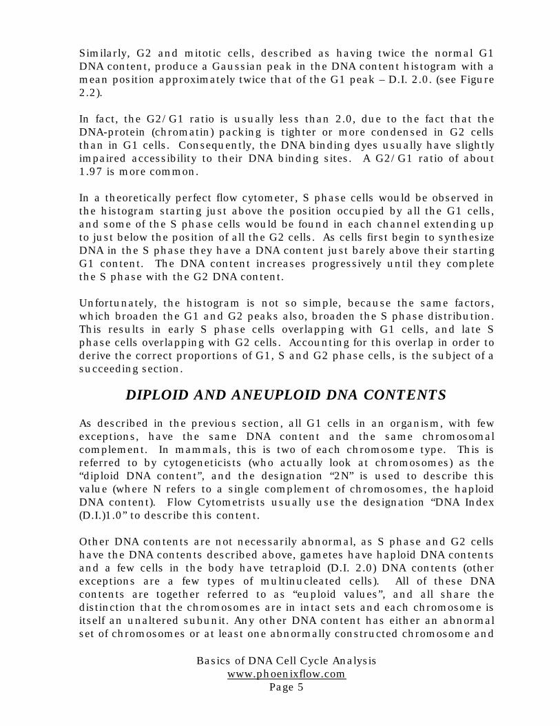
Similarly, G2 and mitotic cells, described as having twice the normal G1DNA content, produce a Gaussian peak in the DNA content histogram with amean position approximately twice that of the G1 peak – D.I. 2.0. (see Figure2.2).

In fact, the G2/G1 ratio is usually less than 2.0, due to the fact that theDNA-protein (chromatin) packing is tighter or more condensed in G2 cellsthan in G1 cells. Consequently, the DNA binding dyes usually have slightlyimpaired accessibility to their DNA binding sites. A G2/G1 ratio of about1.97 is more common.

In a theoretically perfect flow cytometer, S phase cells would be observed inthe histogram starting just above the position occupied by all the G1 cells,and some of the S phase cells would be found in each channel extending upto just below the position of all the G2 cells. As cells first begin to synthesizeDNA in the S phase they have a DNA content just barely above their startingG1 content. The DNA content increases progressively until they completethe S phase with the G2 DNA content.

Unfortunately, the histogram is not so simple, because the same factors,which broaden the G1 and G2 peaks also, broaden the S phase distribution.This results in early S phase cells overlapping with G1 cells, and late Sphase cells overlapping with G2 cells. Accounting for this overlap in order toderive the correct proportions of G1, S and G2 phase cells, is the subject of asucceeding section.

DIPLOID AND ANEUPLOID DNA CONTENTS

As described in the previous section, all G1 cells in an organism, with fewexceptions, have the same DNA content and the same chromosomalcomplement. In mammals, this is two of each chromosome type. This isreferred to by cytogeneticists (who actually look at chromosomes) as the“diploid DNA content”, and the designation “2N” is used to describe thisvalue (where N refers to a single complement of chromosomes, the haploidDNA content). Flow Cytometrists usually use the designation “DNA Index(D.I.)1.0” to describe this content.

Other DNA contents are not necessarily abnormal, as S phase and G2 cellshave the DNA contents described above, gametes have haploid DNA contentsand a few cells in the body have tetraploid (D.I. 2.0) DNA contents (otherexceptions are a few types of multinucleated cells). All of these DNAcontents are together referred to as “euploid values”, and all share thedistinction that the chromosomes are in intact sets and each chromosome isitself an unaltered subunit. Any other DNA content has either an abnormalset of chromosomes or at least one abnormally constructed chromosome and


is referred to as an “aneuploid” (literally other than euploid) DNAconstitution.

Since whole cell or whole nucleus DNA flow cytometry does not measure orexamine chromosomes, flow cytometry cannot tell whether a cell, which hasa DNA Index of 1.0, has a normal chromosomal constitution, and so itshould properly be referred to it as “indistinguishable from diploid”.

Similarly, a cell with a DNA Index of 2.0 could be a “G2 cell”, a tetraploidcell, or an aneuploid cell that has abnormal chromosomes. This is properlytermed as a DNA content “indistinguishable from tetraploid”.

Flow cytometry can detect changes in chromosomes when a population ofcells with a DNA content which is not a multiple of DNA Index 1.0 isobserved, as this requires that either the numbers or the composition ofchromosome(s) have been altered. Since the term “aneuploid” really impliesthat chromosomes have been evaluated, when just DNA content has beenmeasured by flow cytometry it should more properly be referred to as“DNA-aneuploid” to signify this fact.

DNA aneuploid cell populations are almost always, but not exclusively,associated with malignant tissues. Exceptions that must be noted are somebenign tumors (e.g. endocrine adenomas) and some premalignant epithelialcells (e.g. dysplastic epithelium in ulcerative colitis or colon adenomas).

When a malignancy is distinguishable as DNA-aneuploid by flow cytometry,histogram analysis almost invariably shows a mixture of aneuploid anddiploid cells in the tumor. The diploid cells consist of lymphocytes,endothelial cells, fibroblasts and other stromal elements, which are alwayspresent to a greater or lesser degree.Both the malignant and the stromal cells have some subset of cellsproceeding through the progressive G1 → S → G2 → M stages (the stromal Sand G2 phases are usually much smaller than those of malignant cells) andso a DNA content histogram of an aneuploid tumor usually has twooverlapping cell cycles, a complication to the cell cycle analysis, but onewhich MultiCycle has been especially designed to deal with.

CELL CYCLE ANALYSIS OF DNA CONTENTHISTOGRAMS

DNA content histograms require mathematical analysis in order to extractthe underlying G1, S, and G2 phase distributions; methods for this analysishave been developed and refined over the past two decades. Methods toderive cell cycle parameters from DNA content histograms range from simple


graphical approaches to more complex deconvolution methods using curvefitting.

All of the simpler methods are based upon the assumption that the G1 andG2 phase fractions may be approximated by examining the portions of thehistogram where the G1 or G2 phases have less overlap with S phase. Thereare two such approaches. The first is to calculate the area under the left halfof the G1 curve, and the right half of the G2 curve, and multiply each by two(i.e. reflecting these about the peak mean); what remains is S phase. Thesecond approach is to use only the center-most portion of the S phasedistribution, and extrapolate this leftward to the G1 mean and rightward tothe G2 mean. What remains on the left is G1 and on the right is G2. Thesemethods can be reasonably accurate when one cell cycle is present and thehistogram is optimal in shape. Both methods assume that the G1 and G2peaks are symmetrical (DNA staining variability in tissues does not alwaysprovide this) and that the midpoint (mean) of each peak can be preciselyidentified. Because of the overlap of G1 and G2 peaks with the S phase, themean of these peaks is not always at their maximal height (mode), especiallyfor the G2. If a second overlapping cell cycle is also present, then the overlapof the two cell cycles usually precludes safe use of these methods. Inaddition, modeling of debris and aggregates is usually not a part of thesesimpler graphical approaches.

The most flexible and accurate methods of cell cycle analysis are based uponbuilding a mathematical model of the DNA content distribution, and thenfitting this model to the data using curve-fitting methods. The most wellestablished model, proposed by Dean and Jett (1974) is based upon theprediction that the cell cycle histogram is a result of the Gaussianbroadening of the theoretically perfect distribution (Figure 2.2). Theunderlying distribution can be recovered or “deconvoluted” by fitting the G1and G2 peaks as Gaussian curves and the S phase distribution as aGaussian-broadened distribution. As originally proposed, the shape of thisbroadened S phase distribution is modeled as a smooth second-orderpolynomial curve (a portion of a parabola, y = a + bx + cx2). The model canbe simplified by using a first-order polynomial curve (a broadened trapezoid,i.e., S phase modeled by a tilted line, y = a + bx) or a zero-order curve (abroadened rectangle, S phase modeled as a flat line, y = a). When the qualityof the histogram is less than ideal, especially if G1 or G2 peaks are non-Gaussian (broadened bases, skewed or having shoulders), then thesimplified models may give results that are less affected by artifacts thatincrease the overlap of G1, S, and G2 peaks. This often is the case inanalysis of clinical samples, as described in a subsequent section. In thiscase, a conservative approach is suggested, with a zero, or perhaps firstorder S phase, unless there is high confidence in the quality of thehistogram.


Some experimentally derived S phase distributions (usually from culturedcells) are more complex, and several alternative schemes have been proposedto model such distributions. The most flexible model is that of fitting S phaseby the sum of Gaussians (Fried, 1976), in which the S phase is fit by a seriesof overlapping Gaussian curves. In this model each of the Gaussian curvescan be of any height. Therefore, the shape of the S phase is extremelyflexible, and this model can fit S phase distributions that have complexshapes. This is also a primary drawback in practical use of this or similarmodels, however. The very flexible S phase shape allows accurate fitting ofany artifacts in the data, and allows increased ambiguity in fitting the regionof S near G1 and G2 (i.e., the areas of greatest overlap of G1 and S, and Sand G2). A generally successful compromise was suggested by Fox (1980),who added one additional Gaussian curve to Dean and Jett's polynomial Sphase model. Fox's model provides a more flexible S phase shape, but stillretains the smoothness of the S phase that is characteristic of the Dean andJett model. It is especially suited to cell cycle analysis of populations highlyperturbed or synchronized by drug treatments. Fox's model is available inMultiCycle under the name “Synchronous S” (see Chapter 7).

Curve fitting models are almost universally fit to the histogram data by useof least square fitting. The fitting model is used to generate a mathematicalexpression, or function, for the predicted histogram distribution. Thefunction has a number of parameters (usually between 7 and 22) that mustbe adjusted to give the optimum concordance between the fitting model andthe observed data. Since the fitting function used by the model is not asimple linear equation, nonlinear least squares analysis is utilized. Anexcellent description of methods of nonlinear least squares analysis, andsample computer subroutines, is provided by Bevington (1969). The mostcommonly used technique of nonlinear least squares analysis in theseapplications is that described by Marquardt (1963). All of the nonlinear leastsquare fitting techniques are iterative: successive approximations are made,in which the parameters in the fitting model equations are revised and the fitto the data is successively improved. When no further improvement isobtained, the fit has converged, and is theoretically optimal. Goodness of fitis usually quantified by the chi square statistic, χ

σ2 2

2=∑ −( )yfit ydatai i

i, or the

reduced chi square statistic, χνχ2 2

= degrees of freedeom which measure the deviation ofthe fitting function from the data. The speed of the least square fitting isdetermined by the efficiency in searching for and finding the optimumcombination of fitting parameter values. The Marquardt algorithm uses anoptimized strategy for searching for the lowest chi square value along the n-dimensional “surface” defined in the space of the chi-square vs. n fittingvariables.


An advantage of the least square fitting methods is that the models can bedirectly extended to analysis of two or even three overlapping cell cycles. Theoverlapping model components are mathematically deconvoluted to yieldindividual cell cycle estimates. An additional advantage of curve-fittingmethods is that they tend to be less dependent upon the initial or “startingparameters” used to begin the fitting process. Such parameters includeinitial estimates of peak means and CVs, as well as the limits of the region ofthe histogram included in the fit. When the cell cycle and debris model ismost accurate in fitting the data, the result is least dependent on startingvalues, and inter-operator variation in results is reduced (Kallioniemi, et al.,1991).

It has been important to recognize that DNA content histograms from tumortissue are often far from optimal (broad CVs, high debris, and aggregation)or complex (multiple overlapping peaks and cell cycles), and frequentlycontain artifactual departures from expected shapes (e.g., skewed and non-Gaussian peak shapes). This is even truer when analyses are derived fromformalin-fixed specimens. When a skewed G1 peak or a peak with a “tail” onthe right side extends visibly into the S phase, S phase estimates should beused with extreme caution (Shankey, et al., 1993a).

An important aspect of the analysis of imperfect histograms is the ability toreduce the model's complexity by using simplifying assumptions to reducethe number of model parameters being fit. This may reduce the ability of themodel to fit the finer details of a histogram, but it also reduces the possibilityof incorrect fitting of the data. As described above, some models may assumethat a skew or broad base in G0 or G1 peaks is part of the S phase, whichcan lead to an overestimation of the true S phase. More conservative modelsmay be more accurate in situations where CVs are wide or peaks are not wellresolved, when multiple peaks are extensively overlapping, or whenbackground aggregates and debris is high. These situations are more fullydescribed in later sections. The Dean and Jett algorithm may be used with azero (broadened rectangle), or first order S phase polynomial (broadenedtrapezoid), instead of the more flexible, but error-prone second-orderpolynomial. Additional constraints can be imposed to require that the CVs ofthe G2 and G1 peaks be equal (they are usually very similar), or the CVs ofDNA diploid and aneuploid peaks can be made equivalent, or the G2/G1ratios can be constrained to have a user-supplied value, based upon pastlaboratory experience. Please refer to Chapter 8 - Fitting Options, foradditional information on these alternatives.

Finally, as described below, especially careful attention to fitting of thebackground aggregates and debris is also required in order to maximize thereliability of cell cycle analysis of complex histograms.


FITTING OF BACKGROUND “DEBRIS” AND EFFECTSOF NUCLEUS SECTIONING

Almost all cell or nuclear suspensions analyzed by DNA content flowcytometry contain some damaged or fragmented nuclei (debris) resulting inevents, usually most visible to the left of the diploid G1, which are not fit bythe G1, S or G2 compartments. In samples that are derived from freshtissues or cells, most of these “debris” signals are at the left side of thehistogram and fall rapidly to baseline. In the best case, the debris signal isinsignificant in the portion of the histogram occupied by the cell cycle.Unfortunately this is often not the case, and it becomes very important toinclude modeling of the debris curve in the computer analysis in order tosubtract the effects of the underlying debris from the cell cycle fitting.

The conventional assumption in debris fitting is that the rapidly decliningbackground debris curve can be fit by an exponential function (e-kx). Thereare two primary reasons why a simple exponential curve does not usuallyprovide an accurate fit:

1) The shape of most debris curves is not actually exponential. It ismore common to observe a component that rapidly declines with increasingDNA content and then a portion, which declines more slowly, or plateaus.This more slowly declining portion therefore has a much greater effect uponthe cell cycle fitting than is otherwise predicted from an exponential curve.

2) Debris is a result of degradation, fragmentation, or actual cutting ofnuclei, and so extends only leftward (to smaller DNA contents) from eachDNA content position. Therefore, the shape of the debris curve is dependentupon where the peaks in the DNA histogram are, and the debris cannot be fitindependently of the cell histogram. Since the S phase is the lowest andbroadest cell cycle compartment in the histogram, S phase calculations arethe most effected by both of these considerations.

To illustrate these two points, examine the effects of applying differentmodels to a histogram derived from paraffin embedded tissue (Figure 2.3).Figure 2.3A shows fitting of a simple exponential curve to the debris regionleft of the G1 peak. This model does not recognize that much of the debrisresults from fragments of G1 nuclei, and thus it predicts either too much ornot enough debris over the S and G2 phase positions, depending on thefitting region selected.

A more sophisticated model of exponential debris is incorporated intoMultiCycle. Taking into account that debris components extend onlyleftward from the DNA curve position the MultiCycle model assumes thateach DNA content position is associated with the production of exponentialdebris which extends leftward from that position. Because of the different


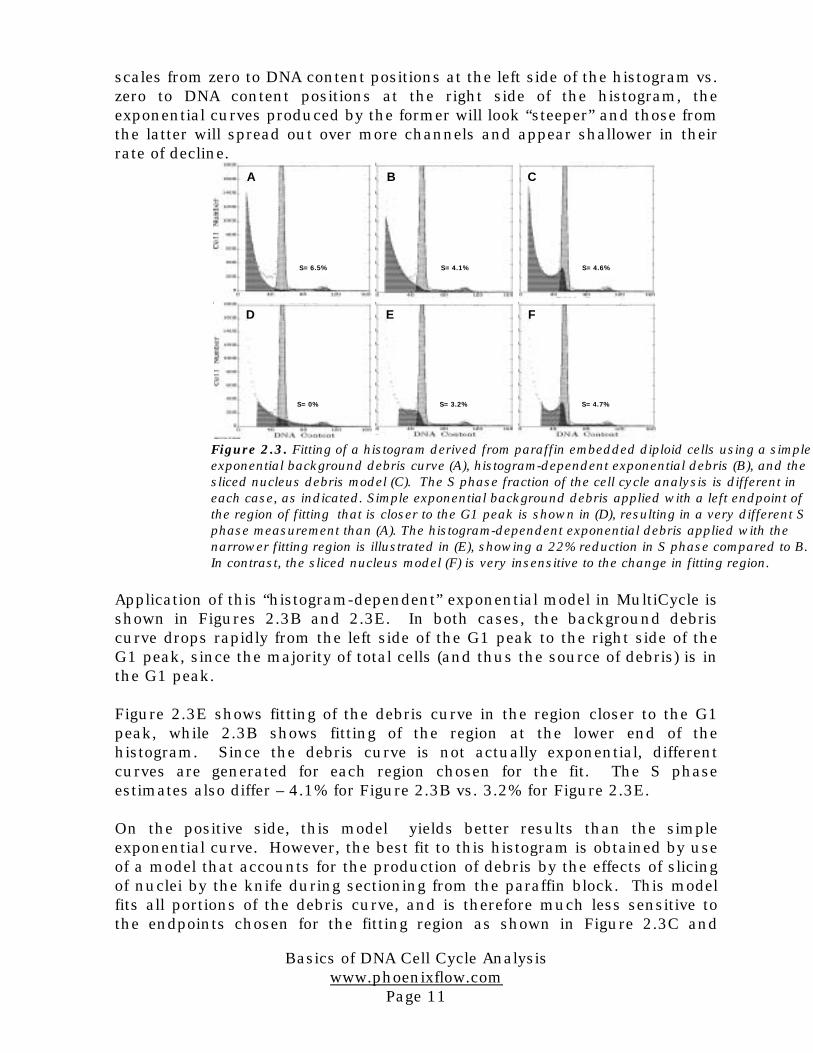
scales from zero to DNA content positions at the left side of the histogram vs.zero to DNA content positions at the right side of the histogram, theexponential curves produced by the former will look “steeper” and those fromthe latter will spread out over more channels and appear shallower in theirrate of decline.

Application of this “histogram-dependent” exponential model in MultiCycle isshown in Figures 2.3B and 2.3E. In both cases, the background debriscurve drops rapidly from the left side of the G1 peak to the right side of theG1 peak, since the majority of total cells (and thus the source of debris) is inthe G1 peak.

Figure 2.3E shows fitting of the debris curve in the region closer to the G1peak, while 2.3B shows fitting of the region at the lower end of thehistogram. Since the debris curve is not actually exponential, differentcurves are generated for each region chosen for the fit. The S phaseestimates also differ – 4.1% for Figure 2.3B vs. 3.2% for Figure 2.3E.

On the positive side, this model yields better results than the simpleexponential curve. However, the best fit to this histogram is obtained by useof a model that accounts for the production of debris by the effects of slicingof nuclei by the knife during sectioning from the paraffin block. This modelfits all portions of the debris curve, and is therefore much less sensitive tothe endpoints chosen for the fitting region as shown in Figure 2.3C and

A B C

D E F

S= 6.5%

S= 0%

S= 4.1% S= 4.6%

S= 4.7%S= 3.2%

Figure 2.3. Fitting of a histogram derived from paraffin embedded diploid cells using a simpleexponential background debris curve (A), histogram-dependent exponential debris (B), and thesliced nucleus debris model (C). The S phase fraction of the cell cycle analysis is different ineach case, as indicated. Simple exponential background debris applied with a left endpoint ofthe region of fitting that is closer to the G1 peak is shown in (D), resulting in a very different Sphase measurement than (A). The histogram-dependent exponential debris applied with thenarrower fitting region is illustrated in (E), showing a 22% reduction in S phase compared to B.In contrast, the sliced nucleus model (F) is very insensitive to the change in fitting region.


2.3F. The utility of this model, especially in analysis of paraffin-derivednuclei, is described below.

Analysis of paraffin preserved cells has become an increasingly importantpart of DNA flow cytometry. Not only is it possible to conduct retrospectiveresearch on such material, thereby establishing relationships of flowcytometry results to long-term patient follow up, but in many cases freshtissue is not available and the analysis of material extracted from paraffinbecomes very important in the clinical setting.

In order to derive useful cell cycle information, care must be exercised in theisolation of nuclei and in the computer modeling of the cell cycle analysis.As part of the process of extraction of nuclei from paraffin blocks, sectionsare usually cut with a microtome at a thickness near 50 µm, and sectioningof nuclei is an unavoidable consequence. These nuclear fragments can havea substantial artifactual effect upon S phase calculations, but amathematical model of the production of sliced nuclei as part of the cell cycleanalysis can help to correct for this effect.

Nuclei in the path of the knife used for sectioning tissue in paraffin blocksare expected to be cut randomly into two portions. If the nuclei wereconsidered in a simple model to be identical cubes randomly cutperpendicularly to one face, then the volume of each randomly cut portionwould have an equal probability of being from near-zero to nearlyfull-volume.

In such a model, a histogram of the volume distribution of a mixture of cutand uncut nuclei would consist of a full-volume peak and a flat continuumto the left ranging from full volume to zero. This is a simplified model ofcourse, but when first introduced in MultiCycle in 1988, it allowed muchbetter fitting of this type of debris than was previously attainable. In fact, itusually requires close inspection of the fitted curves in order to observe thedifference between this and the more refined model described in Figure 2.4.


Since nuclei are actually much closer to spheres or oblate ellipsoids inshape, in a more exact model there would tend to be a somewhat greaterfraction of smaller portions produced, as the rounded ends of the nucleiproduced “crescents” of smaller volume when cut, and of course, theremaining “halves” would be correspondingly larger portions. A histogram ofvolumes resulting from random slicing would thus produce a distributionwhich extended from zero to full-volume, but with a concave rather than aflat distribution, as shown in Figure 2.4. Bagwell et al. (1990) have in factshown that this “spherical” modeling yields the identical result as thatderived for ellipsoids.

This model is implemented in MultiCycle to correct for this effect inbackground debris analysis. For DNA content distributions resulting fromanalyses of cycling cells, mixtures of diploid and aneuploid nuclei (or both)the above model of the effects of cutting nuclei can be implemented byconsidering each channel of the distribution to be a discrete population ofDNA contents for which a certain proportion are cut by random probabilitiesand therefore form a flat-concave continuum to the left of that channel. Theprobability of a nucleus being cut should be proportional to its radius; inMultiCycle the approximation is made that nuclear volume is proportional toDNA content (e.g., S phase and G2 phase nuclei are larger than G1 nuclei).

Figure 2.4. Production of cut portions of nuclei by sectioning with aknife. In the simplest case of spherical nuclei, for a nuclear diameterof “r”, if the knife cuts the nucleus at a distance “h” from an edge, thenthe nuclear volume of this cut section is given by the equation shown.For randomly produced cuts over many nuclei, the theoreticaldistribution of sizes is shown in the histogram at the bottom (the right


The process of least squares fitting is used to determine the probability ofnuclear cutting that yields the best fit to the data. Because small nucleardebris may result from degenerating cells and other fragmentation besidescutting with the microtome, an additional exponential component of the typedescribed previously is also added to the “background” distribution,primarily influencing the left-most portion of the histogram fitting.

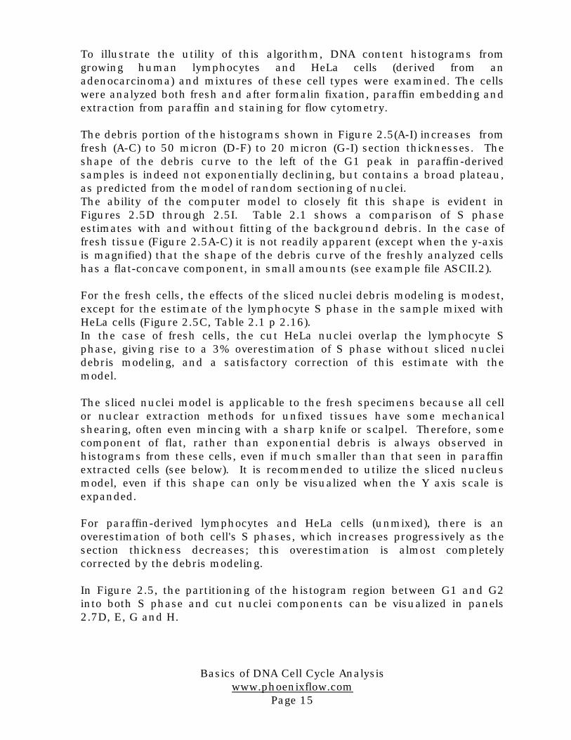
Figure 2.5 below (A-I). Sliced nucleus debris modeling in cell cycle analysis of lymphocytes (A, D, G),HeLa cells (B, E, H) and mixtures of these cells (C, F, I). Analyses were performed on fresh cells (A, B, C),paraffin embedded cells sectioned at 50 microns (D, E, H), and paraffin embedded cells sectioned at 20microns (G, H, I). The debris component of the fitted model is shown by the horizontally hatched portion,and S phase is diagonally hatched.


To illustrate the utility of this algorithm, DNA content histograms fromgrowing human lymphocytes and HeLa cells (derived from anadenocarcinoma) and mixtures of these cell types were examined. The cellswere analyzed both fresh and after formalin fixation, paraffin embedding andextraction from paraffin and staining for flow cytometry.

The debris portion of the histograms shown in Figure 2.5(A-I) increases fromfresh (A-C) to 50 micron (D-F) to 20 micron (G-I) section thicknesses. Theshape of the debris curve to the left of the G1 peak in paraffin-derivedsamples is indeed not exponentially declining, but contains a broad plateau,as predicted from the model of random sectioning of nuclei.The ability of the computer model to closely fit this shape is evident inFigures 2.5D through 2.5I. Table 2.1 shows a comparison of S phaseestimates with and without fitting of the background debris. In the case offresh tissue (Figure 2.5A-C) it is not readily apparent (except when the y-axisis magnified) that the shape of the debris curve of the freshly analyzed cellshas a flat-concave component, in small amounts (see example file ASCII.2).

For the fresh cells, the effects of the sliced nuclei debris modeling is modest,except for the estimate of the lymphocyte S phase in the sample mixed withHeLa cells (Figure 2.5C, Table 2.1 p 2.16).In the case of fresh cells, the cut HeLa nuclei overlap the lymphocyte Sphase, giving rise to a 3% overestimation of S phase without sliced nucleidebris modeling, and a satisfactory correction of this estimate with themodel.

The sliced nuclei model is applicable to the fresh specimens because all cellor nuclear extraction methods for unfixed tissues have some mechanicalshearing, often even mincing with a sharp knife or scalpel. Therefore, somecomponent of flat, rather than exponential debris is always observed inhistograms from these cells, even if much smaller than that seen in paraffinextracted cells (see below). It is recommended to utilize the sliced nucleusmodel, even if this shape can only be visualized when the Y axis scale isexpanded.

For paraffin-derived lymphocytes and HeLa cells (unmixed), there is anoverestimation of both cell's S phases, which increases progressively as thesection thickness decreases; this overestimation is almost completelycorrected by the debris modeling.

In Figure 2.5, the partitioning of the histogram region between G1 and G2into both S phase and cut nuclei components can be visualized in panels2.7D, E, G and H.


When analyzed fresh, HeLa cells showed an S phase fraction of 26%. Whenthe same cells were analyzed after paraffin embedding, but withoutcompensation for effects of nuclear slicing, the S phase fraction was 29 to34%, depending upon the thickness of sectioning (Table 2.1). This effect onS phase estimation is due to the fact that S and G2 phase nuclei are also cutduring sectioning, and some of the cut fragments produced underlie the Sphase compartment distribution, adding to its apparent size and altering itsshape.

Applying the model for correction yields S phase estimates of 26-27% forboth 50 micron and 20-micron sections, closer to the results obtained withfresh cells. Similar results are obtained with cultured lymphocytes (Table2.1), however because there are fewer S and G2 phase cells, the S and G2phase corrections are of smaller magnitude.

Much more dramatic effects of nuclear slicing are seen in histograms inwhich there are two cycling populations with different DNA contents. Whenlymphocytes and Hela cells are mixed; many of the sliced Hela nuclei overlapthe lymphocyte cell cycle distribution and result in an artifactually highestimate of the lymphocyte S phase compartment; this is readily visible in 50micron sections (Figure 2.5F) and is even more pronounced in 20 micronsections (Figure 2.5I). For these cell mixtures, inclusion of the slicednucleus model in the cell cycle fitting produces a result which closely fits theraw data, and at both 50 micron and 20 micron section thicknesses themodel produces S phase estimates which are closer to that of the fresh cells(Table 2.1), although correction of this effect in 20 micron sections is onlypartial.

It is also shown in Table 2.1 that the standard deviation of S phaseestimates is generally smaller when the debris modeling is applied thanwhen it is not applied (i.e., reproducibility is improved). An additionalconsequence of the inclusion of the correction for sliced nuclei is that asmall part of the breadth of the G1 peak is accounted for by the effect ofslicing; at 50 micron section thicknesses the CV of the Hela G1 peakaveraged 5.3 without the sliced nucleus model, and 4.7 with the model.Table 2.1. S phase estimates (S + S.D.) without and with (in parentheses) sliced nucleicorrection (n = 3).

HeLa Lymphocyte Mixed HeLa Lymphocyte

Fresh 26.2 ± .4(25.7 ± .5)

5.5 ± .3(5.2 ± .3)

27.5 ± .8(27.7 ± 1.0)

8.7 ± .1(5.6 ± 0.4)

50 micronparaffin

29.6 ± 2.0(26.6 ± 1.4)

7.1 ± 1.1(5.4 ± .7)

33.7 ± 5.0(28 ± .3)

28.9 ± 2.8(6.1 ± 2.5)

20 micronparaffin

33.8 ± 1.0(26.9 ± .8)

12.8 ± 3.8(6.6 ± 1.1)

43.1 ± 6.8(31.8 ± 3.8)

41.6 ± 5.8(18.3 ± 2.6)


In conclusion, the data presented in this section strongly suggests that useof the sliced nucleus modeling will provide more accurate estimates of Sphase, especially for paraffin derived cells. The final knowledge of how greatan improvement this may be will come from studies performed by the user.Kallioniemi et al. (1991), for example, have found that for node-negativestage I-II breast cancer, the relative risk (RR) of death for high S phasetumors was 3.1 times greater than for low S phase tumors when analyseswere made without background subtraction; the prognostic distinctionimproved to a RR of 4.5 when using MultiCycle's sliced nucleus model. Forcancer of the prostate the RR of high vs. low S phase increased from 3.1 to5.3 using the sliced nucleus model.

FITTING AND CORRECTION FOR THE EFFECTS OFCELL OR NUCLEAR AGGREGATION

In the ideal flow cytometric analysis, a cell or nuclear suspension is free ofaggregates or clumps, and the consideration of the cell cycle and debris issufficient to fit the data. In the majority of “real” histograms, however,careful inspection will reveal evidence of cell aggregation.

“Doublets” of G1 cells will overlie the G2 peak and are difficult to distinguishon the histogram, however triplets will be seen at D.I. 3.0, quadruplets atD.I. 4.0, etc. Not only will the G1 cells aggregate, but S and G2 and nuclearfragments (debris) will also aggregate with G1 cells and with each other. Theeffects of aggregation are more complex when a sample contains aneuploidas well as diploid cells, as aggregates of diploid and aneuploid cells with eachother will occur.

The sources of aggregation can be varied. In some cases disaggregation oftissues will be incomplete and aggregates will remain. Even if disaggregationis initially complete, some preparative procedures for flow cytometry, such asthose which employ ethanol or other solvent fixation, or any procedurewhich uses centrifugation, may reintroduce aggregates.

The conventional approach towards the management of aggregation and itseffects has centered on attempts to distinguish aggregates by the alteredpulse shape which they may produce when illuminated by a focused laserbeam. Subsequent analysis of the DNA histogram is gated on the pulseshape distribution.


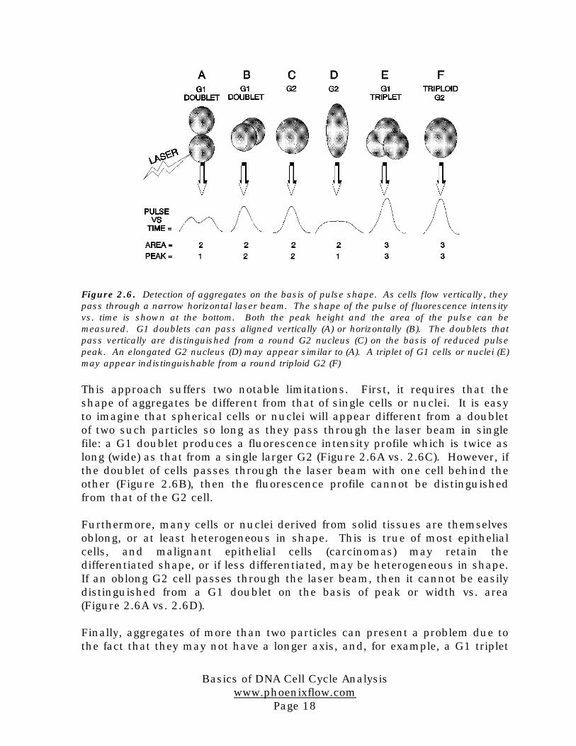
Figure 2.6. Detection of aggregates on the basis of pulse shape. As cells flow vertically, theypass through a narrow horizontal laser beam. The shape of the pulse of fluorescence intensityvs. time is shown at the bottom. Both the peak height and the area of the pulse can bemeasured. G1 doublets can pass aligned vertically (A) or horizontally (B). The doublets thatpass vertically are distinguished from a round G2 nucleus (C) on the basis of reduced pulsepeak. An elongated G2 nucleus (D) may appear similar to (A). A triplet of G1 cells or nuclei (E)may appear indistinguishable from a round triploid G2 (F)

This approach suffers two notable limitations. First, it requires that theshape of aggregates be different from that of single cells or nuclei. It is easyto imagine that spherical cells or nuclei will appear different from a doubletof two such particles so long as they pass through the laser beam in singlefile: a G1 doublet produces a fluorescence intensity profile which is twice aslong (wide) as that from a single larger G2 (Figure 2.6A vs. 2.6C). However, ifthe doublet of cells passes through the laser beam with one cell behind theother (Figure 2.6B), then the fluorescence profile cannot be distinguishedfrom that of the G2 cell.

Furthermore, many cells or nuclei derived from solid tissues are themselvesoblong, or at least heterogeneous in shape. This is true of most epithelialcells, and malignant epithelial cells (carcinomas) may retain thedifferentiated shape, or if less differentiated, may be heterogeneous in shape.If an oblong G2 cell passes through the laser beam, then it cannot be easilydistinguished from a G1 doublet on the basis of peak or width vs. area(Figure 2.6A vs. 2.6D).

Finally, aggregates of more than two particles can present a problem due tothe fact that they may not have a longer axis, and, for example, a G1 triplet


(D.I. = 3) may not be distinguishable from a triploid G2 (D.I. = 3) (Figure 2.6Evs. 2.6F).

Figure 2.7A shows fixed HEL cells, a hematopoietic cell with a roughlyspherical shape. As with most peak/area analyses, a diagonal line is drawn,with the assumption that aggregates will fall below the line (i.e., their pulsepeak value will be lower than non-aggregates for a given pulse area). Figure2.7A shows that for HEL cells, a large population of doublets does fall belowthe line, although some particles with DNA content above the G2 value lieabove the line and could be undiscriminated aggregates.

Figure 2.7B Figure 2.7A Figure 2.7C

Figure 2.7E Figure 2.7D Figure 2.7F

Figure 2.7 (A-F) shows the application of “doublet” discrimination on the basis of pulsepeak vs. pulse area analysis for several cell types. Pulse shape “doublet discrimination”applied to HEL cells (A); colonic mucosal cells (B); nuclei from a breast adenocarcinoma ,before (C) and after trituration (D); and nuclei derived from a high-grade astrocytoma,before (E) and after (F) trituration. In each case, the region above the diagonal line wasused for gating to attempt to remove aggregates. Further analysis of results is shown inFigures 2.9 - 11. Analyses performed on an Ortho Cytofluorograf with a 5µm high laserbeam


Figure 2.7B shows a similar analysis for nuclei derived from normal humancolon mucosa minced in a detergent solution. Many of these nuclei are fromepithelial cells and are elongated in shape, while some are stromal cells,including lymphocytes, which are more spherical. The distribution of G1and G2 cells on the plot of peak vs. area is very variable in the peak value,the expected result from the mixture of round and oblong cells.

It is very difficult to see where on this plot the diagonal should be placed inorder to exclude aggregates; in essence many of the single epithelial nucleihave the pulse shape of round cell doublets, and doublets of epithelial nucleimay not be formed end-to-end, and thus would not look much different thansinglets by pulse shape.

Figures 2.7C and 2.7D show a somewhat more intermediate pattern foranalysis of an aneuploid adenocarcinoma of the breast. A diagonal line isshown that does appear to result in most of the G1 triplets and aggregateswith DNA content greater than the aneuploid G2 being below the line, andthus excluded from the gated analysis.

Figure 2.7D shows the same cells after trituration by syringing 18 timesthrough a 26-gauge needle. Appreciable aggregation still remains, mostbelow the line, however, as in panel 2.7C, some aggregates appear to remainabove the line.

Figures 2.7E and 2.7F show nuclei derived from an aneuploid astrocytoma,before and after syringing, respectively. As for the breast cancer, thediagonal line cannot be placed in a position which appears to exclude allaggregates (without excluding most or all of the G1 nuclei).

Limited attempts to detect aggregates have been made in the past usingsoftware. Sometimes this has been attempted by adding an extra peak tothe cell cycle model to fit the triplet peak position. This is of very limitedutility, since it does not allow for the following:

1) The fitting of much more complicated patterns of aggregation whichresults from G1, S and G2 interactions, as well as clumping of diploid withaneuploid cells.

2) Compensating for the effects of aggregates which cannot be easily fitas separate peaks because they overlie the cell cycle (including doubletswhich may overlap G2). This would be possible if one could estimate theproportion of these aggregates based upon the proportions of otheraggregates that are better separated and visualized.


In order to allow the software to more completely discern the effects ofaggregation, and to compensate for these effects, a theory and model whichallows a generalized approach to computer fitting of aggregation in DNAhistograms has been developed for MultiCycle.

The basis of the MultiCycle model is the assumption that cell aggregation is,or appears to be, a random event. It is assumed that any two cells or nucleiwill aggregate with each other with a certain probability. On the assumptionthat this probability is the same for all cells, the distribution of doublets,triplets, quadruplets, etc. follows rules, and the net “aggregate histogram”has a characteristic shape which is predicted by random probabilisticaggregation formation.

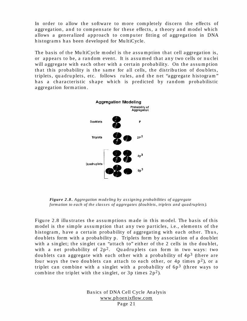
Figure 2.8 illustrates the assumptions made in this model. The basis of thismodel is the simple assumption that any two particles, i.e., elements of thehistogram, have a certain probability of aggregating with each other. Thus,doublets form with a probability p. Triplets form by association of a doubletwith a singlet; the singlet can “attach to” either of the 2 cells in the doublet,with a net probability of 2p2. Quadruplets can form in two ways: twodoublets can aggregate with each other with a probability of 4p3 (there arefour ways the two doublets can attach to each other, or 4p times p2), or atriplet can combine with a singlet with a probability of 6p3 (three ways tocombine the triplet with the singlet, or 3p times 2p2).

Figure 2.8. Aggregation modeling by assigning probabilities of aggregateformation to each of the classes of aggregates (doublets, triplets and quadruplets).


The constants 2, 4 and 6 are derived here in the simplest fashion; it is quitepossible that the “real” constants might be somewhat different. However,from an empirical view, the assumptions above result in a satisfactorymodeling of aggregation.

The key to finding the histogram of the distribution of all possible aggregatesis to let the computer find all possible combinations of one cell or nucleuswith another which can form an aggregate of a particular DNA content. Thedoublet distribution, D(i), for example, may be mathematically derived fromthe cell distribution without aggregation, Y(i), by the formula:

D(i)= p · j

i

k

i

= =∑ ∑

1 1

Y(j) · Y(k) (for all j+k=i).

Where Y(i) is the cell distribution without aggregation.Similarly, the triplet distribution, T(i), is given by:

T(i)= 2p2 · j

i

k

i

= =∑ ∑

1 1

D(j) · Y(k) (for all j+k=i).

and the quadruplet distribution, Q(i), is given by:

Q(i)= 4p3 · j

i

k

i

= =∑ ∑

1 1

D(j) · D(k)

+ 6p3 · j

i

k

i

= =∑ ∑

1 1

T(j) · Y(k) (for all j+k=i).

And, finally, if it is assumed that calculation of aggregates of orders higherthan quadruplets is unnecessary (they have only a minimal effect), the netdistribution of all aggregates is given by:

Aggregates(i)= D(i) + T(i) + Q(i).

Notice that there is only one unknown in the above equations, the value ofthe probability of aggregation, p.

MultiCycle uses the least squares fitting technique to determine the value of“p” which gives the best fit to the data. The multiple iteration fitting processallows the non-aggregated cell distribution to be determined withprogressively improving accuracy as the aggregate distribution derived fromthe above equations is subtracted from the observed total histogram.

An example of this fitting is shown in Figure 2.9, using the histogramderived from the ungated DNA area analysis of the astrocytoma presented inFigure 2.7E. Note that in 2.9B the events to the right of the aneuploid G1

are fit as part of the aggregate “background”, and that the shape of thisaggregate distribution is correctly modeled.


More importantly, however, observe that over the region of the diploid andaneuploid cell cycles theaggregation background distribution fits several peaks within the histogram,and predicts additional aggregation events in the regions overlying S and G2phases.

The net result is that there is an excellent fit to the large numbers of peaksin the data (some being due exclusively to aggregation) and additionally, thatboth S and G2 phase fractions resulting from fitting with this model arelower than if aggregation was not modeled.

Figure 2.9B

Figure 2.9A

Figure 2.9 (A-C).Application of the

aggregation model to theastrocytoma shown inFigure 2.7C (withoutgating). Figure (A)

shows the raw DNAcontent histogram.

Figure (B) (10X scale)shows the total

background fitting(horizontal hatching),including debris and

aggregates. Diploid andaneuploid S phases are

shown by diagonalhatching, and GaussianG1 and G2 peaks areshown by solid lines.

The total fit is indicatedby the dashed line.

Figure (C) (20X scale)shows the individual

components of thebackground fit: slicednucleus debris (solidline at left), doublets(vertical hatching),triplets (diagonal

hatching) andquadruplets (stippling).The total background fit

is indicated by adashed line.

Figure 2.9C


Figure 2.9C shows an expanded view of the components which compose thebackground distribution shown in panel 2.9B. At the left of the histogram,the debris predicted by the sliced nucleus model is seen; this curve declinesprogressively to the right, as seen previously in Figure 2.5. The doubletdistribution (vertical stripes) is seen to be very complex in shape, reflectingthe fact that all histogram components (diploid G1, S and G2, aneuploid G1,S and G2) are predicted to aggregate with each other.

It is apparent that this distribution is so complex that to try to model theaggregation peak-by-peak would be impractical. It is a powerful feature ofthe MultiCycle aggregation modeling that complex distributions are fit asreadily as simple ones.

The triplet distribution is shown with diagonal stripes in Figure 2.9C; it hasan overall higher DNA content than the doublets, but there is extensiveoverlap.

There are, in total, fewer triplets than doublets, a consequence of their lowerprobability of formation. Similarly, the quadruplet distribution is higher inDNA content, and even less abundant than triplets, but overlaps the tripletdistribution to a larger extent.

In order to compare the effects on cell cycle analysis of 1) aggregationmodeling, 2) pulse processing and gating, and 3) trituration by syringing, theexperiments shown in Figures 2.10, 2.11 and 2.12 were performed.

Nuclei were isolated from an adenocarcinoma of the breast (Figures 2.7C andD and Figure 2.10), a high grade astrocytoma (Figures 2.7E and F andFigure 2.11) and normal colon mucosa (Figure 2.7B and Figure 2.12) bymincing in the presence of detergent and DAPI DNA stain. Aliquots of eachsample were subjected to either 4 or 18 passages through a 26-gauge needle.


In addition, whole cells were isolated from the astrocytoma by digestion incollagenase with teasing and mechanical agitation followed by ethanolfixation. Each sample was analyzed as both a gated pulse shape “doubletdetected” (above the diagonal in Figure 2.7) histogram and an ungated DNAhistogram. Each resulting histogram was analyzed with aggregationmodeling and without aggregation modeling (the “regular” model).

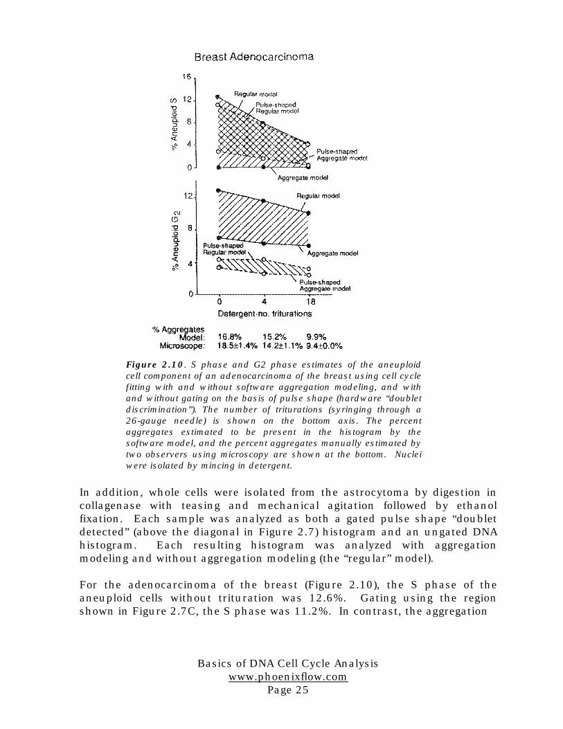
For the adenocarcinoma of the breast (Figure 2.10), the S phase of theaneuploid cells without trituration was 12.6%. Gating using the regionshown in Figure 2.7C, the S phase was 11.2%. In contrast, the aggregation

Figure 2.10. S phase and G2 phase estimates of the aneuploidcell component of an adenocarcinoma of the breast using cell cyclefitting with and without software aggregation modeling, and withand without gating on the basis of pulse shape (hardware “doubletdiscrimination”). The number of triturations (syringing through a26-gauge needle) is shown on the bottom axis. The percentaggregates estimated to be present in the histogram by thesoftware model, and the percent aggregates manually estimated bytwo observers using microscopy are shown at the bottom. Nucleiwere isolated by mincing in detergent.


software model applied to the ungated data reduced the S phase estimate tozero.The aggregate model calculated that 16.8% of the events were aggregates.Manual counting of aggregates by microscopy (two independent observers)showed a mean of 18.5% aggregates, in good agreement with the softwarealgorithm. Because some of the aggregates were removed in the gatedhistogram, when the aggregate model is applied to it, the S phase estimate isnot reduced as much as in the ungated histogram.

With progressive trituration, aggregation was reduced (software and manualestimates remaining in agreement), and S phase estimates without

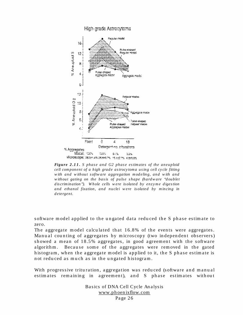
Figure 2.11. S phase and G2 phase estimates of the aneuploidcell component of a high grade astrocytoma using cell cycle fittingwith and without software aggregation modeling, and with andwithout gating on the basis of pulse shape (hardware “doubletdiscrimination”). Whole cells were isolated by enzyme digestionand ethanol fixation, and nuclei were isolated by mincing indetergent.


aggregation modeling also declined. The estimate with aggregation modelingremained at zero. As microscopy showed that almost half the aggregateswere still present after 18 syringings, it seems probable that if furtherdisaggregation of nuclei had been possible, the regular S phase estimatewould have declined much further, perhaps also to zero.

The effect on G2 phase estimates, shown in Figure 2.10, illustrates thatgating removes substantial amounts of events in the aneuploid G2 position.The aggregate model applied to the ungated histograms shows a reductionalso, but not to the level seen in the gated histograms. The aggregationmodel applied to the ungated histograms yields an estimate which variesonly slightly with extent of trituration (syringing).

A plausible interpretation of these results is that gating removes not onlysome aggregates, but also some legitimate G2 events. Resetting the gatingregion to remove fewer cells would result in the elimination of even feweraggregates over the S phase.A very similar result was obtained with cells from the astrocytoma (Figure2.11). Trituration was more successful in this example in removingaggregates. The higher estimate of aggregation from microscopicexamination may have been due to the presence of cells which visuallyappeared adjacent but which did not remain aggregated within the flowcytometer. Once again, the software aggregation modeling resulted in an Sphase estimate for the aneuploid cells which was almost independent of thedegree of aggregation, and was similar for fixed and unfixed cells.The regular S phase estimate was progressively reduced with trituration.This rate of decline suggests the possibility that had mechanicaldisaggregation been complete, then the regular model estimate would haveequaled the aggregate model estimate. The fixed whole cell preparationappeared to have fewer G2 cells by all estimates. The reason for this is notknown, however it is possible that release of G2 cells by enzymatic digestionwas less complete than by detergent isolation.


Finally, Figure 2.12 shows results obtained with normal colon mucosal cells.These cells have a low S phase. There is not a great difference between anyof the models, although there appears to be a slight decline in all S phaseestimates with trituration.

The more interesting results with these cells concern the G2 phaseestimates. With increasing trituration, a large reduction in the G2 phase isseen in the ungated “regular model”. Gating on the basis of pulse shapereduces the G2 estimate by 1%, but does not otherwise change the variationwith trituration. In contrast, the software aggregation model shows a lowerand more consistent G2 estimate.

In summary, the experiments shown in Figures 2.10-12 demonstrate that, ingeneral, for cell types which have heterogeneous and elongated nuclei, thesoftware aggregation model produces cell cycle estimates that are closer tothe values seen in triturated, disaggregated samples.

Figure 2.12. S phase and G2 phase estimates of normalcolon mucosal nuclei using cell cycle fitting with andwithout software aggregation modeling, and with andwithout gating on the basis of pulse shape (hardware“doublet discrimination”).


At present, there is not sufficient data to know whether hardware andsoftware aggregate compensation might in some circumstances be usedtogether (sequentially). Thus, it is suggested that software aggregatemodeling be applied to non-gated histograms.

Finally, it should be noted that microscopic enumeration of aggregationrequires careful discrimination between merely adjacent vs. adherent cells.Some of the discrepancies between microscopic enumeration and thesoftware estimate could be due to difficulties in distinguishing adjacent fromadherent cells. If there is a need to quantify aggregation (even if there is noattempt to compensate for its effects), then the software algorithm may bemore consistent. Identification of samples which contain higher amounts ofaggregation should allow renewed attempts to triturate and disaggregate thesample, and a repeat of the flow cytometric analysis.

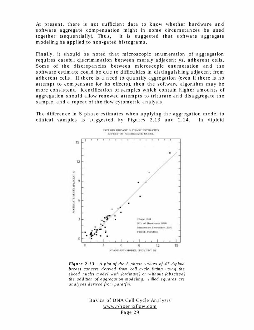
The difference in S phase estimates when applying the aggregation model toclinical samples is suggested by Figures 2.13 and 2.14. In diploid

Figure 2.13. A plot of the S phase values of 47 diploidbreast cancers derived from cell cycle fitting using thesliced nuclei model with (ordinate) or without (abscissa)the addition of aggregation modeling. Filled squares areanalyses derived from paraffin.


specimens, fewer aggregates overlie S phase (those that do are primarilyaggregates of debris and G1 cells). S phase estimates in diploid breast

cancers were reduced, on the average to 94.4% of the standard modelestimate (Figure 2.13), a decline which averaged only 0.89% absolute Sphase units, with a maximum decline of 3.4% S phase units. Aneuploid Sphase estimates, on the other hand, were reduced to 85.4% of the standardestimate, an average decline of 2.5% S phase units, with a maximum declineof 14.5% S phase units.

Note that in Figure 2.14 there are a number of examples of S phaseestimates reduced from the high range (e.g. 13%) to the intermediate range

(e.g. 7%), or from the intermediate range (e.g. 7%) to the low range (e.g. 2%).

Figure 2.14. A plot of the S phase values of 56aneuploid breast cancers derived from cell cycle fittingusing the sliced nuclei model with (ordinate) or without(abscissa) the addition of aggregation modeling. Filledsquares are analyses derived from paraffin.


QUANTITATION OF BACKGROUND AGGREGATES

AND DEBRIS

The relative proportion of events analyzed by the flow cytometer that consistof cell or nuclear debris or aggregates is highly variable. The debris isgenerally higher in paraffin processed tissue, due to nuclear slicing, and indegenerating or necrotic tissue, but these magnitudes are difficult to predict.To address the need for a quantitative measure of aggregates and debris, theDNA Cytometry Consensus Conference defined a parameter termedBackground Aggregates and Debris (BAD), defined as the proportion of thehistogram events between the leftmost G1 and the rightmost G2 that ismodeled as debris or aggregates. The reason that this parameter is definedin this manner, rather than as the total percent debris and aggregates in theentire histogram, is that left and right end-points of a histogram are variableand arbitrary, depending on instrument settings. The proportion of debris inthe histogram is especially sensitive to variation in the left limit of dataacquisition. The BAD is unaffected by histogram endpoints. It is, however,very much dependent on the choice of histogram modeling. For greatestaccuracy and inter-laboratory comparison, it is suggested that histogram-dependent sliced nucleus and aggregation models of background correctionbe utilized. MultiCycle will calculate and display the % BAD, and will use theBAD as one indicator of cell cycle fitting reliability.

ANALYSIS OF APOPTOSIS

There is increasing interest in measurement of cells undergoing programmed“self-destruction” via apoptosis. During apoptosis, the nuclear DNA isfragmented. The fragments can be removed from cells by one of a number ofstaining protocols, making apoptotic cells visible as a peak below the G1DNA content. Usually, this peak is approximately Gaussian in shape andcan be quantitated using the “overlapped peak” MultiCycle fitting option.


Figure 2.15 illustrates that the degree of retention of apoptotic DNAfragments within the cell can be influenced by the staining buffer, and thatthis can be quantitated by histogram analysis. Note that in analysis ofapoptotic peaks the lower range limit for peak searching should be set belowthe apoptotic peak, and the left limit of the debris fitting region should beplaced to the left of the apoptotic peak, so that the apoptotic peak is notmistaken for or confused with debris.

BEYOND SINGLE PARAMETER ANALYSIS: DNA VS.IMMUNOFLUORESCENCE

Univariate DNA content analysis offers simplicity of sample preparation, and,with care, accurate cell cycle measurements can be obtained. Considerablefuture potential, however, will be derived from bivariate analyses, where oneparameter is DNA content and the other is an immunofluorescent probe.In the analysis of solid tissues, important classes of targets for antibodyprobes will be cell cycle associated antigens, and oncogene products. Inorder to demonstrate that careful methods of data analysis and cell cycleanalysis are still important in this emerging area, an example of analysis ofDNA content vs. Ki-67 antibody staining is shown.

Figure 2.15. Analysis of Apoptotic populations of cells using the “OverlappedPeak” fitting option. The apoptotic peak in Panel A represents 43.6% of cells,and has 41.7% the DNA staining intensity of diploid cells. In panel B, the cellshave been incubated in a more hypotonic buffer, and the apoptotic peak has only24.2% the staining intensity of diploid cells. Data courtesy of Z. Darzynkiewiczand F. Traganos.


Figure 2.16 shows the analysis of human esophageal epithelial cells (thisexample happens to come from metaplastic columnar Barrett's epithelium)with the antibody Ki-67. Expression of the target for this antibody is cellcycle associated: low in quiescent G0 cells and early G1 cells, and higher inlate G1, S and G2 cells.

Figure 2.16 (A-C). Ki-67 analysis ofhuman Barrett's esophagus. Negativecontrol stained with irrelevant primaryand PE-secondary antibody, as well asDAPI DNA stain (A); staining with Ki-67antibody and PE-secondary antibodyvs. DNA (B); and (A)subtracted from(B), shown in (C). The Y-axis is Ki-67fluorescence and the X-axis is DNAcontent.


Comparing the negative control (A) with the Ki-67 stained cells (B), one cansee that the Ki-67 stained cells have a portion of G1 positive cells, a largeproportion of S phase cells positive, and a distinct sub-population of positiveand negative G2 cells. The negative “S” phase cells include aggregates ofdebris and G1 cells, and the negative “G2” cells include aggregated G1doublets. In order to quantitate the proportion of Ki-67 positive G1 phasecells (activated G1) or Ki-67 positive S phase cells (true S?) one needs toidentify positive from negative Ki-67 staining. Merely drawing a line at apoint which visually appears to be appropriate has numerous drawbacks,not the least of which is its lack of reproducibility.

An alternative software approach is shown in (C), in which the negativecontrol Ki-67 fluorescence histogram at each interval of the DNA content(X-axis) is subtracted from the corresponding X-axis interval of the positive

staining distribution (subtraction is performed using the cumulativesubtraction algorithm described by Overton [1988

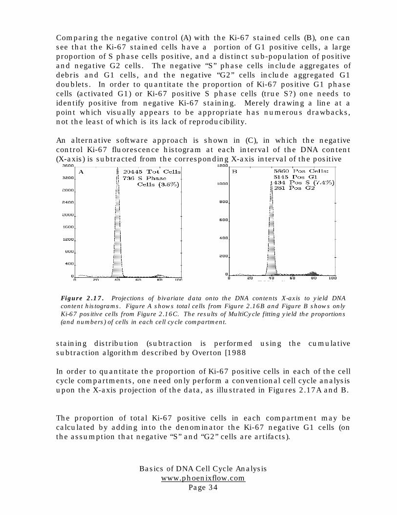
In order to quantitate the proportion of Ki-67 positive cells in each of the cellcycle compartments, one need only perform a conventional cell cycle analysisupon the X-axis projection of the data, as illustrated in Figures 2.17A and B.

The proportion of total Ki-67 positive cells in each compartment may becalculated by adding into the denominator the Ki-67 negative G1 cells (onthe assumption that negative “S” and “G2” cells are artifacts).

Figure 2.17. Projections of bivariate data onto the DNA contents X-axis to yield DNAcontent histograms. Figure A shows total cells from Figure 2.16B and Figure B shows onlyKi-67 positive cells from Figure 2.16C. The results of MultiCycle fitting yield the proportions(and numbers) of cells in each cell cycle compartment.

introduction to dna cell cycle analysis

Documents