Introduction to Green functions andmany-body perturbation theory

Last updated 20 March 2013

Contents

1 Motivation 21.1 Connection to experiments . . . . . . . . . . . . . . . . . . . . . . . . . . . . 21.2 Divergences in the standard perturbation theory . . . . . . . . . . . . . . . . 3

2 The single-particle retarded Green function and its spectral function 42.1 Retarded, advanced, “greater”, and “lesser” single-particle Green functions . 42.2 The meaning of 〈· · ·〉 and the time dependence . . . . . . . . . . . . . . . . . 52.3 Some other forms of the Green functions . . . . . . . . . . . . . . . . . . . . 6

2.3.1 Transformations to other bases . . . . . . . . . . . . . . . . . . . . . 72.3.2 Green functions in other bases . . . . . . . . . . . . . . . . . . . . . . 72.3.3 k-space Green function in translationally invariant systems . . . . . . 82.3.4 Fourier transformed Green functions (in the time-frequency domain) . 8

2.4 Example: Green function for noninteracting electrons . . . . . . . . . . . . . 82.5 The Lehmann representation . . . . . . . . . . . . . . . . . . . . . . . . . . . 102.6 The spectral function . . . . . . . . . . . . . . . . . . . . . . . . . . . . . . . 11

2.6.1 Sum rule and physical interpretation . . . . . . . . . . . . . . . . . . 122.6.2 Spectral function for noninteracting fermions and Fermi liquids . . . 132.6.3 Relation to momentum distribution (through weighted sum over ω)

and to density of states (through sum over k) . . . . . . . . . . . . . 14

3 Imaginary-time (Matsubara) Green functions 143.1 Motivation . . . . . . . . . . . . . . . . . . . . . . . . . . . . . . . . . . . . . 143.2 Imaginary-time single-particle Green function . . . . . . . . . . . . . . . . . 153.3 Periodicities in imaginary time. Fourier series and Matsubara frequencies . . 163.4 The connection between imaginary-time and retarded Green functions . . . . 173.5 Example: Noninteracting fermions . . . . . . . . . . . . . . . . . . . . . . . . 183.6 Equation of motion approach for Matsubara Green functions . . . . . . . . . 19

3.6.1 General Hamiltonians . . . . . . . . . . . . . . . . . . . . . . . . . . . 193.6.2 Quadratic Hamiltonians . . . . . . . . . . . . . . . . . . . . . . . . . 203.6.3 Solution as perturbation series . . . . . . . . . . . . . . . . . . . . . . 21

1

4 Electrons in a disordered potential 224.1 Motivation . . . . . . . . . . . . . . . . . . . . . . . . . . . . . . . . . . . . . 224.2 The impurity scattering Hamiltonian . . . . . . . . . . . . . . . . . . . . . . 224.3 Perturbation series solution for the single-particle Matsubara Green function 234.4 Averaging over impurity locations . . . . . . . . . . . . . . . . . . . . . . . . 244.5 Impurity-averaged Matsubara Green function: Perturbation series and Feyn-

man diagrams . . . . . . . . . . . . . . . . . . . . . . . . . . . . . . . . . . . 264.5.1 Feynman rules for diagrams contributing to G(n)(k) . . . . . . . . . . 264.5.2 Low-order Feynman diagrams . . . . . . . . . . . . . . . . . . . . . . 27

4.6 Irreducible diagrams, the self-energy, and the Dyson equation . . . . . . . . . 284.7 Low-density weak-scattering approximation for the self-energy . . . . . . . . 314.8 The impurity-averaged retarded Green function and its spectral function . . 334.9 An example of linear response theory and two-particle Green functions: The

Kubo formula for the electrical conductivity . . . . . . . . . . . . . . . . . . 344.10 Calculating the conductivity from the Kubo formula . . . . . . . . . . . . . . 38

5 Concluding remarks 41

1 Motivation

The Green function methods for quantum many-body systems were mainly developed in the1950’s and early 60’s. Before plunging into the formalism we briefly summarize some mainmotivations behind this development.

1.1 Connection to experiments

Here we will be very sketchy. Consider an experiment in which one exposes the system tosome disturbance (whose strength is controlled by some external applied field f(r, t)) andmeasures the response of the system. When the applied field is weak one expects the responseto depend linearly on the applied field. This is called linear response. The “proportionalityfactor” is the associated response function. The basic equations can be shown to be (herewe suppress all variables except the time variables)

Htot = H − f(t)O, (1)

〈O(t)〉 = 〈O〉+

∫ ∞

−∞χ(t− t′)f(t′)dt′, (2)

χ(t− t′) = −i〈[O(t), O(t′)]〉θ(t− t′). (3)

Here H (Htot) is the Hamiltonian of the system in the absence (presence) of the applied fieldf(t), 〈O(t)〉 is the response (in terms of the operator O) of the system to the field, with 〈O〉being the expectation value of O in the absence of the applied field (which often vanishes).The function χ(t) is a retarded response function (retarded means that it’s only nonzero fort > t′, i.e. cause comes before effect). Other names sometimes used for such a quantity issusceptibility, correlation function or Green function. (As we will see there are many other,

2

related quantities that are also called Green functions). Note that the expectation value in(3) is with respect to the undisturbed system, i.e. in the absence of the applied field.

For example the electrical conductivity σ(q, ω) is related to a response function where theO’s are given by the current operators, i.e. a retarded current-current correlation function.(Here the variables q and ω arise from taking Fourier transforms in space and time.) If timeallows we will study the conductivity σ(q, ω) in more detail later (see Secs. 4.9 and 4.10).

Retarded Green functions and functions related to these are thus central objects tocalculate in many-body theory for comparing with experiments.

1.2 Divergences in the standard perturbation theory

One of the important early problems was to find the ground state energy of a gas of electronsinteracting via the long-ranged Coulomb interaction in 3 dimensions. (To ensure chargeneutrality this gas was embedded in a positive and uniform background charge.) Considerthe kinetic energy and potential energy of this electron gas as a function of r0, the averagedistance between two electrons (in 3D r0 ∝ n−1/3 where n is the electron density). Onecan show that the kinetic energy per electron goes like 1/r2

0. and that the typical Coulombinteraction energy per electron goes like 1/r0. Thus for small r0, i.e. a high-density gas, thekinetic energy dominates over the interaction energy, and one might hope that it is possibleto treat the Coulomb interaction as a perturbation to the kinetic energy.1 Thus in this limitone might hope that the ground state energy can be expressed in terms of a power series inthe small dimensionless parameter rs = r0/aB (aB is the Bohr radius) like

E0 =K

r2s

[1 + brs + cr2s + . . .] (anticipated, but turns out to be not quite right) (4)

where K, a, b, c, etc. are constants. Indeed, 1st order perturbation theory gives a termof the form brs in this series. But if one goes one step further and considers 2nd orderperturbation theory, one finds a contribution which diverges like

∫0 dq/q, where q is the

momentum transfer in the Fourier transform vq of the Coulomb interaction (vq ∝ 1/q2).That is, there is a logarithmic divergence from the lower limit 0 of the momentum transfers.This divergence is associated with the long range of the Coulomb interaction. Furthermore,if one examines higher order terms in the perturbation series one finds that they divergeeven more strongly. Thus standard perturbation theory appears to be worthless.

On physical grounds, however, one does of course expect the energy of the interactingelectron gas to be a finite and well-defined number, and no phase transitions occur as one“turns on” the repulsive interactions, so this failure of standard perturbation theory appearsjust to be a signal that the energy does not have a standard power series expansion in rs. In1957 Gell-Mann and Bruckner resolved this issue by using the recently developed many-bodyperturbation theory. Essentially what they did was to sum all the most divergent terms inthe series (an infinite number of them) before doing the momentum integrals, and showedthat one could then arrive at a result which was well-defined and finite (this is called aresummation of the perturbation series). They found that there was a term in the series forE0 which is ∝ ln rs, and thus indeed is not analytic at rs = 0.

1This assumes at the very least that the interaction doesn’t cause any drastic changes to the system, suchas a phase transition.

3

The solution of this problem thus requires one to include an infinite number of terms inthe perturbation theory. Clearly one needs to develop a new method to be able to do thisin an efficient way, and this is one of the main strengths of many-body perturbation theory.We will also see other examples where one needs to include an infinite number of terms inthe perturbation theory.

2 The single-particle retarded Green function and itsspectral function

Most response functions, e.g. the conductivity, involve retarded two-particle Green functions,in which the operator O in (3) involves the product of two creation/annihilation operators.However, we will start by discussing single-particle Green functions, as they are the simplestones. Essentially, single-particle Green functions involve operators O which are a single cre-ation or annihilation operator. In the fermionic case, the commutator in (3) is then replacedby an anticommutator in the definition of the retarded single-particle Green function.

2.1 Retarded, advanced, “greater”, and “lesser” single-particleGreen functions

The retarded single-particle Green function is defined as

GR(x, t; x′, t′) ≡ −iθ(t− t′)〈[ψ(x, t), ψ†(x′, t′)]±〉. (5)

The upper sign is for fermions, when [A, B]+ ≡ A, B is the anticommutator. The lower signis for bosons, when [A, B]− ≡ [A, B] is the ordinary commutator. Furthermore, x ≡ (r, σ),so that ψ†(x) ≡ ψ†

σ(r) creates a particle at position r with spin projection σ (if the particlehas a spin degree of freedom). We also define an advanced Green function as

GA(x, t; x′, t′) ≡ +iθ(t′ − t)〈[ψ(x, t), ψ†(x′, t′)]±〉. (6)

Note that the retarded function is nonzero only for t > t′ and the advanced function isnonzero only for t < t′. It is also convenient at this point to define two other types of Greenfunctions, referred to as “G-greater” and “G-lesser”:

G>(x, t; x′, t′) ≡ −i〈ψ(x, t)ψ†(x′, t′)〉, (7)

G<(x, t; x′, t′) ≡ −i(∓)〈ψ†(x′, t′)ψ(x, t)〉. (8)

In G< the upper sign is again for fermions and the lower for bosons. The retarded andadvanced Green functions can then be expressed as

GR(x, t; x′, t′) = θ(t− t′)[G>(x, t; x′, t′)−G<(x, t; x′, t′)], (9)

GA(x, t; x′, t′) = θ(t′ − t)[G<(x, t; x′, t′)−G>(x, t; x′, t′)]. (10)

4

2.2 The meaning of 〈· · · 〉 and the time dependence

We will consider a system with a macroscopic number of particles which is in thermodynamicequilibrium at some temperature T (which may be zero or nonzero). The average 〈· · · 〉represents a thermal + quantum average in such a system. In general, there are two kinds ofensembles which may describe such systems: the canonical ensemble and the grand canonicalensemble. Let us summarize these in turn, starting with the simpler one, the canonicalensemble.

In the canonical ensemble the number of particles N in the system is fixed, and thesystem can exchange energy with a reservoir. The average energy of the system is determinedby the temperature T . The quantum statistical-mechanical average of an arbitrary operatorA is in this ensemble given by

〈A〉 =1

Z

∑

n

〈n|A|n〉e−βEn (11)

Here |n〉 refer to the set of (normalized) eigenstates of the Hamiltonian H with eigenvaluesEn, β = 1/kBT , and Z =

∑n e−βEn is the partition function. We can write the expectation

value in a basis-independent way by defining the density matrix (calling it a matrix ismisleading, but that is the standard name; it really is an operator)

ρ =1

Ze−βH (12)

andZ = Tr e−βH . (13)

(Clearly Tr ρ = 1 as required for a density matrix.) With this definition we can write

〈A〉 = Tr(ρA). (14)

In the grand canonical ensemble the system does not have a fixed particle number.Instead, the system can exchange particles (in addition to energy) with a reservoir. Thuswe need to introduce another parameter (in addition to the temperature T ), namely thechemical potential µ, which determines the average number of particles in the system. Thedensity matrix for this ensemble is given by

ρ =1

Ze−β(H−µN) (15)

where the partition function isZ = Tr e−β(H−µN). (16)

Here N is a number operator which counts the total number of particles. With these defini-tions of ρ and Z we again have

〈A〉 = Tr(ρA). (17)

To actually evaluate this trace it is convenient to use the basis consisting of eigenstates of theoperator H − µN . Note that the total number of particles in such an eigenstate is definite(when H conserves the total number of particles), but can take an arbitrary nonnegative

5

value.

In the following we will use the grand canonical ensemble. In regard to this thereare some important things that should be pointed out:

• In this ensemble the time dependence of operators is defined to be determined by theoperator H − µN , not H. This corresponds to measuring all single-particle energieswith respect to the chemical potential µ. Thus we define

A(t) ≡ ei(H−µN)tAe−i(H−µN)t. (18)

• However, to save writing we will still write this as A(t) = eiHtAe−iHt. That is, H herewill be implicitly understood to represent the operator H − µN .

• Similarly, instead of writing e−β(H−µN) we will write e−βH .

• Finally, the eigenstates of the operator H−µN (which we write as H!) will be writtenas |n〉 and the eigenvalues will be written as En. Thus we write

H|n〉 = En|n〉. (19)

As already mentioned above, the number of particles in such a many-body eigenstateis definite but can take any integer value from 0 to ∞.

In summary, whenever we refer to “the Hamiltonian” and “H” in the following, we reallymean H − µN . (This is also what is done in the texts by Coleman and by Bruus andFlensberg when using the grand canonical ensemble.)

2.3 Some other forms of the Green functions

The Green functions defined so far are called space-time Green functions, because theyinvolve the creation and annihilation of particles at definite locations in space and time.We can also define analogous Green functions in other bases than the spatial one (moreprecisely, space-spin basis when the particles have spin). For example, it will in manyproblems, especially those which are translationally invariant in space, be convenient to studyGreen functions which involve creation/annihilation of particles in a definite momentumstate characterized by a momentum k. Depending on the problem at hand, other Greenfunctions, involving creation/annihilation of particles in other types of single-particle states,may also be useful. (For example, if the particles move in some external potential U(x) itmay be convenient to define Green functions which create/annihilate particles in eigenstatesof p2/2m + U(x)). Finally, it is also interesting to Fourier transform the Green functions inthe time-frequency domain (Sec. 2.3.4).

6

2.3.1 Transformations to other bases

To relate these alternative Green functions to the space-time Green functions already defined,we need to know how to transform between bases. Thus we give a short repetition/summaryof how to do this. Consider a basis |ν〉 (e.g. |ν〉 = |k, σ〉). We may write

|x〉 =∑

ν

|ν〉〈ν|x〉 =∑

ν

〈x|ν〉∗|ν〉 =∑

ν

φ∗ν(x)|ν〉, (20)

where φν(x) ≡ 〈x|ν〉 is the single-particle wavefunction in the state |ν〉. Writing |x〉 =ψ†(x)|0〉 and |ν〉 = c†ν |0〉 (where |0〉 is the “vacuum” state containing no particles at all)we then have the following relation between the creation operators in the x-basis and theν-basis:

ψ†(x) =∑

ν

φ∗ν(x)c†ν . (21)

Taking the hermitian conjugate of this gives the relation between the corresponding annihi-lation operators:

ψ(x) =∑

ν

φν(x)cν . (22)

The most relevant example is when |ν〉 = |k, σ〉. Then

ψ†(x) = ψ†σ(r) =

∑

k,σ′

φ∗k,σ′(r, σ)︸ ︷︷ ︸

φk(r)δσ,σ′

c†k,σ′ =∑

k

φ∗k(r)c†kσ =1√Ω

∑

k

e−ik·rc†k,σ (23)

and thus also

ψσ(r) =∑

k

φk(r)ckσ =1√Ω

∑

k

eik·rck,σ. (24)

Here, to arrive at the last expressions in (23) and (24) we have taken the particles to live ina system which is a 3D cube of volume Ω with periodic boundary conditions, so

φk(r) =1√Ω

eik·r. (25)

2.3.2 Green functions in other bases

We will illustrate how Green functions in different bases are related by looking at the retardedsingle-particle Green function. We have

GR(x, t; x′t′) = −iθ(t− t′)〈[ψ(x, t), ψ†(x′, t′)]±〉= −iθ(t− t′)

∑

νν′

φν(x)φ∗ν′(x′)〈[cν(t), c

†ν′(t

′)]±〉

=∑

νν′

φν(x)φ∗ν′(x′)GR(ν, t; ν ′, t′), (26)

where we have defined the single-particle retarded Green function in the ν-basis as

GR(ν, t; ν ′, t′) = −iθ(t− t′)〈[cν(t), c†ν′(t

′)]±〉. (27)

7

2.3.3 k-space Green function in translationally invariant systems

In a system which is translationally invariant in space, the space-time Green functions cannot depend on r and r′ separately, but only on their difference r− r′. In these systems it isnatural to consider the k-space Green function G(k, σ, t; k′σ′, t′), as it becomes diagonal inthe k indices. This can be seen from (26), (23) and (24). We have

GR(x, t; x′, t′) = G(r, σ, t; r′, σ′, t′) =1

Ω

∑

k,k′

eik·re−ik′·r′GR(k, σ, t; k′, σ′, t′)

=1

Ω

∑

k,k′

eik·(r−r′)ei(k−k′)·r′GR(k, σ, t; k′, σ′, t′). (28)

As the lhs only depends on r−r′, the dependence on r′ on the rhs must vanish, which meansthat the k-space Green function is nonzero only when k = k′, i.e. GR(k, σ, t; k′, σ′, t′) =δk,k′GR(k; σ, t; σ′, t′). Thus we get

GR(r − r′, σ, t; σ′, t′) =1

Ω

∑

k

eik·(r−r′)GR(k; σ, t; σ′, t′) (29)

whereGR(k; σ, t; σ′, t′) = −iθ(t− t′)〈[ck,σ(t), c†k,σ′(t

′)]±〉. (30)

2.3.4 Fourier transformed Green functions (in the time-frequency domain)

If the Hamiltonian does not depend explicitly on time, i.e. the Hamiltonian is translationallyinvariant in time, the Green functions will not depend on t and t′ separately, but only on thedifference t − t′. It is then convenient to Fourier transform the Green function in the timevariable. This Fourier transform and its inverse are defined as

G(t) =1

2π

∫ ∞

−∞dω e−iωtG(ω), (31)

G(ω) =

∫ ∞

−∞dt eiωtG(t). (32)

(Here we have suppressed all other variables than the time/frequency variables in the nota-tion.)

2.4 Example: Green function for noninteracting electrons

We will now calculate the k-space Green functions for noninteracting electrons. In this case,the Hamiltonian is given by

H =∑

k,σ

ξkc†k,σck,σ (33)

where ξk = εk − µ and µ is the chemical potential. Because H is diagonal in k and σ (theformer property is due to the system being translationally invariant in space, as there is no

8

external potential in the Hamiltonian), the Green functions will also be diagonal in k andσ. Taking this into account we consider the retarded Green function

GR0 (k, σ; t− t′) = −iθ(t− t′)〈ckσ(t), c†kσ(t′)〉. (34)

The subscript 0 on the Green function refers to the noninteracting nature of the Hamiltonian.To calculate the Green function we need to work out the time dependence of the fermion

operators. Sinceckσ(t) = eiHtckσe

−iHt, (35)

we havedckσ(t)

dt= i[H, ckσ(t)] = ieiHt [H, ckσ]︸ ︷︷ ︸

−ξkckσ

e−iHt = −iξkckσ(t). (36)

Integrating this differential equation gives

ckσ(t) = e−iξktckσ, (37)

c†kσ(t) = eiξktc†kσ. (38)

We see that the time dependence of the operators is very simple for noninteracting electrons.We now get for the greater Green functions:

G>0 (k, σ, t− t′) = −ie−iξkteiξkt′〈ckσc

†kσ〉 = −ie−iξk(t−t′)(1− 〈nkσ〉)

= −ie−iξk(t−t′)(1− nF (ξk)), (39)

where

nF (ω) ≡ 1

eβω + 1(40)

is the Fermi-Dirac distribution function. At zero temperature this becomes nF (ω) = θ(−ω),hence a state k is occupied if εk < µ and empty if εk > µ.

The calculation of the lesser Green function is very similar:

G<0 (k, σ, t− t′) = +i〈c†kσ(t′)ckσ(t)〉 = ieiξkt′e−iξkt〈c†kσckσ〉 = ie−iξk(t−t′)nF (ξk). (41)

The retarded Green function can then be found from (9), which gives

GR0 (k, σ, t− t′) = −iθ(t− t′)e−iξk(t−t′). (42)

Let us next consider the Fourier transform of this function, defined in (32):

GR0 (kσ,ω) = −i

∫ ∞

−∞dt eiωtθ(t)e−iξkt = −i

∫ ∞

0

dt ei(ω−ξk)t. (43)

To make the integral converge at the upper limit we let ω → ω + iη where η = 0+ is apositive infinitesimal. This gives

GR0 (kσ,ω) =

1

ω − ξk + iη. (44)

9

We note that this Green function, considered as a function of ω for fixed k, has a pole atω = ξk− iη, i.e. at the excitation energy ξk of the system, except that the pole is just shiftedinfinitesimally off the real axis in the complex ω-plane and down into the lower half-plane.Thus the Fourier transform of the retarded Green function has the following properties: itis analytic in the upper half-plane, and the location of its poles (all in the lower half-plane)offer information about the excitation energies of the system. In the next section we will seethat these are general features of the Fourier transform of the retarded Green function.

2.5 The Lehmann representation

We will now consider the diagonal Green function GR(ν, t; ν ′, t′) ≡ GR(ν; t, t′) = GR(ν; t− t′)for the fermionic case and derive what is called the Lehmann (or spectral) representation forits Fourier transform GR(ν; ω). We start with

G>(ν; t, t′) = −i〈cν(t)c†ν(t

′)〉. (45)

Next we write the explicit expressions for the average 〈· · · 〉 and for the time dependenceof the operators. The trace involved in the average (see (17)) will be evaluated using thecomplete set of eigenstates |n〉 of H and the associated eigenvalues En. We also insert aresolution of the identity in terms of these eigenstates, i.e. I =

∑m |m〉〈m| inbetween the

operators cν(t) and c†ν(t′). (Note that although we don’t know what these eigenstates are,

we know that they exist, which is sufficient here.) This gives

G>(ν; t, t′) = −i1

Z

∑

n

e−βEn〈n|cν(t)c†ν(t

′)|n〉

= − i

Z

∑

n,m

e−βEn〈n|eiHtcνe−iHt|m〉〈m|eiHt′c†νe

−iHt′|n〉

= − i

Z

∑

n,m

e−βEnei(En−Em)(t−t′) 〈n|cν |m〉︸ ︷︷ ︸〈m|c†ν |n〉∗

〈m|c†ν |n〉

= − i

Z

∑

n,m

e−βEnei(En−Em)(t−t′)|〈m|c†ν |n〉|2. (46)

Following exactly the same steps to calculate G<(ν; t, t′) = i〈c†ν(t′)cν(t)〉, we get

G<(ν; t, t′) =i

Z

∑

n,m

e−βEnei(Em−En)(t−t′)|〈n|c†ν |m〉|2

=i

Z

∑

n,m

e−βEmei(En−Em)(t−t′)|〈m|c†ν |n〉|2 (47)

where in the last expression we interchanged the names of the dummy summation variablesn, m. This gives

GR(ν; t− t′) = θ(t− t′)[G>(ν; t, t′)−G<(ν; t, t′)]

= −iθ(t− t′)1

Z

∑

n,m

(e−βEn + e−βEm

)ei(En−Em)(t−t′)|〈m|c†ν |n〉|2. (48)

10

The Fourier transform of this is

GR(ν,ω) =

∫ ∞

−∞dt eiωtGR(ν, t)

= − i

Z

∑

n,m

(e−βEn + e−βEm

)|〈m|c†ν |n〉|2

∫ ∞

−∞dt θ(t)ei(ω+En−Em)t

= − i

Z

∑

n,m

(e−βEn + e−βEm

)|〈m|c†ν |n〉|2

∫ ∞

0

dt ei(ω+En−Em+iη)t, (49)

i.e.,

GR(ν,ω) =1

Z

∑

n,m

|〈m|c†ν |n〉|2

ω + En − Em + iη

(e−βEn + e−βEm

). (50)

In this calculation we again let ω → ω + iη (where η = 0+) to make the integral convergent.Eq. (50) is the Lehmann representation of GR(ν,ω). One can see that the singularities ofGR(ν,ω) are poles located infinitesimally below the real axis at ω = Em−En− iη (this poleexists provided the matrix element 〈m|c†ν |n〉 *= 0). Hence from the poles of GR(ν,ω) onecan obtain information about the excitation energies Em − En associated with eigenstates|m〉 and |n〉 which are connected through the creation operator c†ν , i.e. eigenstates for whichthe state |m〉 has a finite overlap with the state c†ν |n〉. Here, clearly the eigenstate |m〉 hasa single particle more than the eigenstate |n〉. Thus GR(ν,ω) gives information about thesingle-particle excitation spectrum.

2.6 The spectral function

In this section we will discuss a very important quantity called the (single-particle) spectralfunction A(ν,ω), which is essentially the imaginary part of GR(ν,ω),2

A(ν,ω) ≡ − 1

πIm GR(ν,ω). (51)

Using Eq. (50) and the fact that, for η = 0+ and real x,

Im1

x + iη= − η

x2 + η2= −πδ(x), (52)

we find that

A(ν,ω) =1

Z

∑

n,m

|〈m|c†ν |n〉|2(e−βEn + e−βEm

)δ(ω + En − Em). (53)

It can be shown that GR(ν,ω) can be expressed in terms of the spectral function as follows:

GR(ν,ω) =

∫dω′

A(ν,ω′)

ω − ω′ + iη. (54)

2The prefactor −1/π in (51) is a common, although not unique, convention. Some authors instead takethe prefactor to be −2, which leads to factors of 2π differences in some of the following expressions.

11

A similar relation holds with GR(ν,ω) replaced by the advanced Green function GA(ν,ω) onthe lhs and with +iη replaced by −iη on the rhs. From this one concludes that the Fouriertransforms of the retarded and advanced Green functions are simply complex conjugates ofeach other (for real values of ω): GA(ν,ω) = [GR(ν,ω)]∗. One can also show that

iG>(ν,ω) = 2π A(ν,ω)[1− nF (ω)], (55)

−iG<(ν,ω) = 2π A(ν,ω)nF (ω), (56)

which are known as the fluctuation-dissipation theorem for the fermionic single-particle Greenfunctions. The proofs of Eqs. (54)-(56) will be left to a tutorial.

In the following we will for concreteness take ν = (k, σ).

2.6.1 Sum rule and physical interpretation

We will next show that the spectral function A(kσ, ω) satisfies∫ ∞

−∞dω A(kσ,ω) = 1. (57)

The proof goes as follows:∫ ∞

−∞dω A(kσ, ω) =

1

Z

∑

m,n

|〈m|c†kσ|n〉|2(e−βEn + e−βEm

) ∫ ∞

−∞dω δ(ω + En − Em)

︸ ︷︷ ︸1

=1

Z

∑

m,n

|〈m|c†kσ|n〉|2(e−βEn + e−βEm

)

=1

Z

∑

m,n

〈m|c†kσ|n〉〈n|ckσ|m〉(e−βEn + e−βEm

)

=1

Z

∑

n,m

[e−βEn〈n|ckσ|m〉〈m|c†kσ|n〉+ e−βEm〈m|c†kσ|n〉〈n|ckσ|m〉

]

=1

Z

[∑

n

e−βEn〈n|ckσc†kσ|n〉+

∑

m

e−βEm〈m|c†kσckσ|m〉]

=1

Z

∑

n

e−βEn〈n| (ckσc†kσ + c†kσckσ)

︸ ︷︷ ︸=ckσ ,c†kσ=1

|n〉 =1

Z

∑

n

e−βEn

︸ ︷︷ ︸=Z

= 1. (58)

Eq. (57) is an example of a sum rule. A sum rule is an exact result for the frequency in-tegral of a certain frequency-dependent quantity (typical examples being spectral functionsof retarded Green functions, like A(kσ,ω)). In actual calculations for real systems, one isusually only able to get approximate results for such quantities, which may not satisfy thesum rule exactly. In such cases the extent to which the sum rule is approximately satisfiedcan be a useful measure of the quality of the approximations made.

The property (57) together with the fact that A(kσ, ω) ≥ 0 (which can be seen from (53))suggests that A(kσ, ω) can be interpreted as a probability density. One can say (somewhat

12

loosely speaking for the general interacting case) that A(kσ,ω)dω is the probability that afermion with momentum k has an energy in an infinitesimal energy window dω about ω.

2.6.2 Spectral function for noninteracting fermions and Fermi liquids

Let us now investigate A(kσ, ω) for a system of noninteracting fermions. We already calcu-lated the retarded Green function for this case, GR

0 (kσ, ω), in Eq. (44). It follows that theassociated spectral function is a delta function,

A0(kσ,ω) = δ(ω − ξk). (59)

Thus in this case the spectral function is nonzero only if the argument ω equals ξk, which isthe energy of a particle with quantum numbers (k, σ) appearing in H0. Therefore the energyof the particle is known with certainty when the momentum is given. This certainty is areflection of the fact that in the noninteracting system, the many-body wavefunction is simplygiven by a single Slater determinant involving products of single-particle wavefunctionsφkσ(r) with associated energy ξk = εk − µ. [It should be noted that for any quadraticHamiltonian of the form H0 =

∑ν ξνc†νcν one finds the same result, i.e. A0(ν,ω) = δ(ω−ξν),

so there’s nothing special about choosing ν = (k, σ) here.]In a large class of systems of interacting fermions, known as Fermi liquids, the spectral

function can be written

A(kσ, ω) ≈ Zk

π

(1/2τk)

(ω − ξ∗k)2 + (1/2τk)2+ Aincoherent(kσ,ω). (60)

Here τk is a lifetime, ξ∗k is a renormalized energy, and Zk is a constant which is a positivenumber between 0 and 1. Compared to the noninteracting case, there is still a peak in thespectral function, represented by the first term in (60). However, the peak is now a Lorentzianinstead of a delta function. Also, the width of the peak has broadened, the area under thepeak has decreased (from 1 to Zk), and the single-particle energies are renormalized. Thereis also an additional term Aincoherent(kσ, ω) representing a continuum (i.e. not a peak) whichmust be there if Zk *= 1 for the sum rule (57) to be satisfied.

A finite (i.e. not infinite) lifetime3 τk reflects the fact that in the presence of interactionsthe many-body wavefunction is a sum of many Slater determinants, which can be thought ofas resulting from the fact that the interactions make the fermions scatter between differentsingle-particle states φkσ(r) (i.e. states with different k’s); the lifetime τk is thus a measureof the time between such scattering events. In a Fermi liquid, 1/τk approaches zero very fastas |k| approaches the Fermi momentum kF . As a consequence, fermions close to the Fermisurface scatter very little, which can be shown to imply that treating them as essentiallynoninteracting is still qualitatively correct for many purposes. This is a very significantresult since many experimentally measurable properties are at low temperatures essentiallydetermined by the fermions at or near the Fermi surface. These properties are therefore notqualitatively changed by the electron-electron interactions.

The entities having energy ξ∗k and lifetime τk are called quasi-particles. As alreadynoted, fermion systems in which this picture holds are called Fermi liquids, and the theory

3Note that in the limit τk →∞ the first term in the spectral function again becomes a delta function.

13

describing them is known as Fermi liquid theory (which was first developed phenomenologi-cally by Landau around 1957 and was subsequently given a microscopic foundation throughthe use of many-body perturbation theory in the following years).

We note that the identification and investigation of interacting fermionic systems whichdo not obey Fermi liquid theory is an important research question in current many-bodyphysics. Such non-Fermi liquids by definition have a spectral function which can not beapproximated by the form (60) and as a result they can therefore not be qualitatively un-derstood in terms of a picture of noninteracting fermions. One prominent example of anon-Fermi liquid is the so-called Luttinger liquid which occurs in one spatial dimension.

2.6.3 Relation to momentum distribution (through weighted sum over ω) andto density of states (through sum over k)

We will next find an exact expression for the quantity nν ≡ 〈c†νcν〉 in terms of a (weighted)frequency integral of the spectral function A(ν,ω). We have

nν ≡ 〈c†νcν〉 = −iG<(ν, t = 0) =1

2π

∫ ∞

−∞dω eiω·0

︸︷︷︸=1

· (−i)G<(ν,ω)︸ ︷︷ ︸=2πA(ν,ω)nF (ω)

=

∫ ∞

−∞dω A(ν,ω)nF (ω), (61)

where we used (56). When ν = (kσ) this gives a relation between the momentum distributionfunction nkσ ≡ 〈c†kσckσ〉 and A(kσ,ω):

nkσ =

∫ ∞

−∞dω A(kσ,ω)nF (ω). (62)

For a noninteracting system this gives nkσ =∫∞−∞ dω δ(ω − ξk)nF (ω) = nF (ξk).

Another important quantity is the single-particle density of states D(ω) which is essen-tially the spectral function A(k, ω) summed over all k:

D(ω) =1

Ω

∑

k,σ

A(kσ,ω). (63)

The spectral function A(k, ω) can be measured experimentally by tunneling spectroscopy(in this technique the differential conductance dI/dV at low temperatures gives informa-tion about the density of states D(ω)) and Angle Resolved Photo-Emission Spectroscopy(ARPES). For details see Bruus and Flensberg, Ch. 8.4 and Coleman Ch. 10.7.2 and 10.7.3.

3 Imaginary-time (Matsubara) Green functions

3.1 Motivation

In most interacting systems, calculating physically interesting quantities like e.g. retardedGreen functions and associated spectral functions is highly nontrivial and can usually only be

14

accomplished approximately, e.g. in terms of many-body perturbation theory. For technicalreasons it is useful to introduce what is known as imaginary-time Green functions,as it turns out that direct calculations of the retarded Green functions are impractical atfinite temperatures. As we will see there is a rather simple mathematical relation betweenthe imaginary-time Green functions and the retarded Green functions which allows one toobtain the latter from the former. In this section we develop these results for the case ofsingle-particle Green functions, again focusing mainly on the fermionic case. The imaginary-time formalism is sometimes also referred to as the Matsubara formalism, and we will usethese two names interchangeably.4

3.2 Imaginary-time single-particle Green function

The imaginary-time (or Matsubara) single-particle Green function is defined as

G(ν, τ ; ν ′, τ ′) ≡ −〈Tτ (cν(τ)c†ν′(τ′))〉. (64)

Here τ and τ ′ are real parameters satisfying 0 < τ, τ ′ < β where β = 1/kBT as usual. Thetime dependence of operators in the imaginary-time formalism is defined as

A(τ) ≡ eHτAe−Hτ , (65)

A†(τ) ≡ eHτA†e−Hτ . (66)

Compared to the usual real-time evolution defined in terms of the operators e±iHt, it is asif we had set it = τ . Since τ is real, this corresponds to t being imaginary; hence the name“imaginary-time.” Note that τ being real means that e±τH are not unitary. This has theimportant implication that

A†(τ) *= (A(τ))†. (67)

Thus (65) and (66) are independent definitions and are not each other’s adjoints, unlike thecase for unitary real-time evolution.

The symbol Tτ in (64) is a time ordering operator which puts the operators in chronologi-cal order, with the earliest times furthest to the right, according to the following prescription:

T (cν(τ)c†ν′(τ′)) ≡

cν(τ)c†ν′(τ

′) if τ > τ ′

εc†ν′(τ′)cν(τ) if τ ′ > τ.

(68)

Here ε = −1 if the c’s are fermion operators and ε = +1 if they are boson operators. Thus inthe fermionic case a minus sign is introduced upon interchanging the order of the operatorswhile in the bosonic case there is no sign change.5

When the Hamiltonian is time-independent these Green functions will only depend onthe time difference τ − τ ′ and not on τ and τ ′ individually (as was also the case for the

4There is also another formalism available which in contrast to the Matsubara formalism is only applicableat zero temperature and is therefore called the zero temperature formalism.

5This should not be confused with the standard commutation/anticommutation properties ofbosonic/fermionic operators which in general only apply at equal times, while here the operators are evalu-ated at different times τ and τ ′.

15

real-time Green functions considered in Sec. 2). This allows us to limit our consideration(without any loss of generality) to the function

G(ν, ν ′; τ) ≡ −〈Tτ (cν(τ)c†ν′(0))〉 (69)

where τ can now take values in the interval −β < τ < β.

3.3 Periodicities in imaginary time. Fourier series and Matsubarafrequencies

We will now show that the Matsubara Green functions obey the (anti-)periodicity conditions(here τ < 0)

G(ν, ν ′; τ) = ∓G(ν, ν ′; τ + β) (70)

where the upper (lower) sign is for fermions (bosons). To prove (70) we use the cyclicinvariance of the trace operation,

Tr(ABC . . . XY Z) = Tr(ZAB . . . WXY ) = Tr(Y ZA . . . V WX) etc. (71)

For the fermionic case this gives (τ < 0)

G(ν, ν ′; τ) = −〈Tτ (cν(τ)c†ν′(0))〉 = 〈c†ν′(0)cν(τ)〉

=1

ZTr(e−βHc†ν′e

Hτcνe−Hτ )

=1

ZTr(eHτcνe

−Hτe−βHc†ν′)

=1

ZTr(e−βHeβH

︸ ︷︷ ︸=I

eHτcνe−Hτe−βHc†ν′)

=1

ZTr(e−βHeH(τ+β)cνe

−H(τ+β)c†ν′)

=1

ZTr(e−βHcν(τ + β)c†ν′(0)) = 〈cν(τ + β︸ ︷︷ ︸

>0

)c†ν′(0)〉

= −G(ν, ν ′; τ + β) QED. (72)

The proof for the bosonic case is obviously very similar.We can now use (70) twice to get G(ν, ν ′;−β) = ∓G(ν, ν ′; 0) = (∓)2G(ν, ν ′; β) = G(ν, ν ′; β).

Hence the Matsubara Green function is periodic with period 2β on the interval τ ∈ (−β, β)and can therefore be expanded in a standard Fourier series on this interval, which can bewritten as

G(ν, ν ′; τ) =1

β

∑

n∈Ze−iωnτG(ν, ν ′; iωn), (73)

G(ν, ν ′; iωn) =1

2

∫ β

−β

dτeiωnτG(ν, ν ′; τ). (74)

16

where the frequencies ωn6 are given by ωn = (2πn)/(2β) = πn/β. Actually, because of the

property (70) only a certain subset of the frequency components will be nonzero. This canbe seen by splitting the integral in (74) into one over (−β, 0) and one over (0, β), using (70)in the first region to rewrite it too as an integral over the second region, and using the factthat e−iωnβ = e−iπn = (−1)n:

G(ν, ν ′; iωn) =1

2

∫ 0

−β

dτ eiωnτ G(ν, ν ′; τ)︸ ︷︷ ︸∓G(ν,ν′;τ+β)

+

∫ β

0

dτ eiωnτG(ν, ν ′; τ)

=1

2[∓(−1)n + 1]

︸ ︷︷ ︸

∫ β

0

dτ eiωnτG(ν, ν ′; τ). (75)

For fermions, the bracketed quantity is 1 if n is odd and 0 if n is even, while for bosons it’s1 if n is even and 0 if n is odd. Hence for fermions (bosons) only odd (even) values of ncontribute in the Fourier series, which makes it natural to define

ωn ≡ (2n + 1)π

βfor fermions, (76)

ωn ≡ 2nπ

βfor bosons (77)

where again n runs over all integers for both fermions and bosons. This gives our final resultfor the Fourier representation of the Matsubara Green functions:

G(ν, ν ′; τ) =1

β

∑

ωn

e−iωnτG(ν, ν ′; iωn), (78)

G(ν, ν ′; iωn) =

∫ β

0

dτ eiωnτG(ν, ν ′; τ). (79)

The frequencies ωn are known as Matsubara frequencies. Note that they depend ontemperature. They are discrete at finite temperature but become continuous in the limit ofzero temperature (β → ∞), when the spacing 2π/β between adjacent frequencies goes tozero. It has become customary to denote fermionic Matsubara frequencies by pn or kn andbosonic Matsubara frequencies by qn or ωn, which is a convention we will tend to follow fromnow on.

3.4 The connection between imaginary-time and retarded Greenfunctions

We will next consider how one can obtain a retarded Green function from the correspondingimaginary-time Green function. The key is to calculate the Fourier transform G(iωn) of thelatter; then the retarded function GR(ω) can be found from this by the substitution

iωn → ω + iη (80)

6We have put a tilde on these frequencies because we are going to define a slightly different frequencyvariable ωn below.

17

(where η is a positive infinitesimal), a procedure known as analytic continuation. Thisresult follows from a comparison of the Lehmann representations for the imaginary-time andretarded Green functions. Since we considered the Lehmann representation for the fermionicdiagonal retarded function GR(ν,ω) ≡ GR(ν, ν; ω) in Sec. 2.5 we will here consider theLehmann representation for the corresponding Matsubara function G(ν, ipn) ≡ G(ν, ν; ipn).The result (80) is however valid also for the non-diagonal case, and for bosons, and alsoextends to more complicated Green functions than the single-particle one.

To calculate G(ν, ipn) we first need to find G(ν, τ). Following the same procedure as inSec. 2.5 we have (we consider τ > 0 only as that is sufficient to calculate G(ν, ipn))

G(ν, τ) = −〈cν(τ)c†ν(0)〉

= − 1

Z

∑

n,m

e−βEn〈n|eHτcνe−Hτ |m〉〈m|c†ν |n〉

= − 1

Z

∑

n,m

e−βEne(En−Em)τ |〈m|c†ν |n〉|2. (81)

Thus

G(ν, ipn) = − 1

Z

∑

n,m

e−βEn|〈m|c†ν |n〉|2∫ β

0

dτ e(ipn+En−Em)τ

= − 1

Z

∑

n,m

e−βEn|〈m|c†ν |n〉|2e(ipn+En−Em)β − 1

ipn + En − Em

=1

Z

∑

n,m

|〈m|c†ν |n〉|2

ipn + En − Em(e−βEn + e−βEm), (82)

where we used thateipnβ = −1 (83)

which follows from (76). Comparing (82) with (50) we see that indeed the Matsubara andretarded functions are simply related by (80).

3.5 Example: Noninteracting fermions

In this section we calculate the Matsubara Green function for noninteracting fermions. TheHamiltonian is given by

H0 =∑

ν

ξνc†νcν . (84)

We denote the Matsubara function by G(0)(ν, τ); the superscript 0 reflects the fact thatthe quadratic Hamiltonian is diagonal in the ν-basis; this makes the Matsubara functiondiagonal too. Using that

cν(τ) = eH0τcνe−H0τ = e−ξντcν , (85)

18

we find

G(0)(ν, τ) = −〈Tτ (cν(τ)c†ν(0)〉= −θ(τ)〈cν(τ)c†ν(0)〉+ θ(−τ)〈c†ν(0)cν(τ)〉= −e−ξντ [θ(τ)〈cνc

†ν〉 − θ(−τ)〈c†νcν〉]

= −e−ξντ [θ(τ)(1− nF (ξν))− θ(−τ)nF (ξν)]. (86)

Thus

G(0)(ν, ipn) =

∫ β

0

dτ eipnτG(0)(ν, τ)

= −(1− nF (ξν))

∫ β

0

dτ e(ipn−ξν)τ

=1

ipn − ξν· (−1)(1− nF (ξν))

[e(ipn−ξν)β − 1

]︸ ︷︷ ︸

=1

=1

ipn − ξν(87)

where we used (40) and (83). It is reassuring that if we now let ipn → ω + iη in thisexpression to obtain the retarded Green function, we get the same result (44) as we obtainedearlier when calculating the retarded Green function directly for this case of noninteractingfermions.

3.6 Equation of motion approach for Matsubara Green functions

We will now develop an equation of motion approach to find the Matsubara single-particleGreen function. This involves differentiating the Matsubara Green function with respect toτ , which will lead us to a differential equation obeyed by this function. We will see that forthe case of quadratic Hamiltonians the differential equation is relatively simple in that itonly involves single-particle Green functions. This differential equation can be transformedinto an algebraic equation by Fourier transformation, for which a solution can be found inthe form of an infinite series.

3.6.1 General Hamiltonians

Let us start by considering a fermionic system with a completely general Hamiltonian Hand the Matsubara Green function G(ν, ν ′; τ) where ν is some arbitrary basis:

G(ν, ν ′; τ) = −〈Tτ (cν(τ)c†ν′(0))〉. (88)

Differentiating this with respect to τ gives

d

dτG(ν, ν ′; τ) = − d

dτ

[θ(τ)〈cν(τ)c†ν′(0)〉 − θ(−τ)〈c†ν′(0)cν(τ)〉

]

= −δ(τ)〈(cν(τ)c†ν′(0) + c†ν′(0)cν(τ))︸ ︷︷ ︸

=δνν′ (τ=0)

〉 −[θ(τ)〈 d

dτcν(τ)c†ν′(0)〉 − θ(−τ)〈c†ν′(0)

d

dτcν(τ)〉

]

= −δ(τ)δνν′ −[θ(τ)〈[H, cν(τ)]c†ν′(0)〉 − θ(−τ)〈c†ν′(0)[H, cν(τ)]〉

], (89)

19

i.e.,

− d

dτG(ν, ν ′; τ) = δ(τ)δνν′ + 〈Tτ ([H, cν(τ)]c†ν′(0))〉. (90)

To arrive at this result we used the equation of motion for cν(τ),

dcν(τ)

dτ= [H, cν(τ)] (91)

which follows from (65). Note that the factor δνν′ arose due to the delta function δ(τ) whichallowed us to set τ = 0 in that term and then make use of the equal-time anticommutationrelations.

If the Hamiltonian contains nontrivial interaction terms, such as terms that are quartic inthe creation/annihilation operators (an example would be the Coulomb interaction betweenelectrons), the second term on the rhs of (90) will involve higher-order Green functions thanthe single-particle one (e.g. two-particle Green functions). One can in turn find the equationof motion for these which will involve Green functions of even higher order, and so on. Inorder to make progress, this hierarchy of ever more complicated equations must then be“cut off” at some level by approximating the multi-particle Green function at that level asa product of lower-order Green functions.

In the following we will instead consider the simpler case of a quadratic Hamiltonian.Then, as we will see, the term on the rhs of (90) involving the expectation value of the time-ordered expression will just be another single-particle Green function. Thus in this case theequations of motion for the single-particle Green functions will constitute a “closed” systemof equations.

3.6.2 Quadratic Hamiltonians

Assume that H is quadratic so that it can be written on the form

H =∑

ν′ν

hν′νc†ν′cν (92)

which gives[H, cν(τ)] = −

∑

ν′

hνν′cν′(τ). (93)

Inserting this into (90) one finds

− d

dτG(ν, ν ′; τ) = δ(τ)δνν′ +

∑

ν′′

hνν′′G(ν ′′, ν ′; τ), (94)

which is an equation of motion that only involves single-particle Green functions. Next weseparate H into its diagonal part and non-diagonal parts,

hνν′ = ξνδνν′ + vνν′ (95)

which gives (− d

dτ− ξν

)G(ν, ν ′; τ) = δ(τ)δνν′ +

∑

ν′′

vνν′′G(ν ′′, ν ′; τ). (96)

20

This differential equation can now be turned into an algebraic equation by introducing theFourier transform defined in (78)-(79). The lhs of (96) can then be written (1/β)

∑pn

(ipn−ξν)e−ipnτG(ν, ν ′; ipn). Upon multiplying both sides of the equation by eipmτ and integratingover τ from τ = 0 to τ = β, one arrives at

(ipm − ξν)G(ν, ν ′; ipm) = δνν′ +∑

ν′′

vνν′′G(ν ′′, ν ′; ipm) (97)

where we used7

1

β

∫ β

0

dτ ei(pm−pn)τ = δmn, (98)

∫ β

0

dτ eipmτδ(τ − 0+) = 1. (99)

From (87) we have ipm − ξν = (G(0)(ν; ipm))−1, so that (97) can be rewritten as

G(ν, ν ′; ipm) = G(0)(ν, ipm)δνν′ + G(0)(ν; ipm)∑

ν′′

vνν′′G(ν ′′, ν ′; ipm). (100)

Note that the Matsubara frequency ipm is the same in all the Green functions in this equation,which makes it a little unnecessary to carry it along. To lighten the notation we will thereforedrop it in the following.

3.6.3 Solution as perturbation series

Next we write an ansatz for the solution to Eq. (100) in the form of an infinite series,

G(ν, ν ′) =∞∑

n=0

G(n)(ν, ν ′) (101)

where G(n) contains n powers of the non-diagonal matrix elements vνiνj . When the non-diagonal part is zero, the solution of (100) is clearly just the unperturbed Green function,i.e.

G(0)(ν, ν ′) = G(0)(ν)δνν′ . (102)

7Eq. (99) requires some further explanation. One can regard the delta function δ(τ) in Eq. (90) asthe limit of a Lorentzian with a finite width and centered at τ = 0. It is then clear that only half of thisfunction is inside the integration region, so

∫ β0 dτ eipmτδ(τ) = 1/2. However, the result (90) is in fact not

entirely correct as it stands. If −(d/dτ)G has a delta function contribution at τ = 0, then because of theanti-periodicity (70) it should also have delta function contributions at τ = −β and τ = β with oppositesigns from that at τ = 0. So if we integrate from 0 to β, the delta function at τ = β also gives contribution1/2 (the minus sign in front of the delta function is cancelled by the factor eipmβ = −1 that is also in theintegrand). Thus the total contribution from the two delta functions at τ = 0 and τ = β is 2 · 1/2 = 1. Weget the same result by keeping (90) as it is (i.e. not adding to it the delta function contributions at τ = ±β)and shifting G(τ) by an infinitesimal amount to the right. Then the center of the delta function at τ = 0is shifted to τ = 0+ and thus it lies entirely inside the integration region, giving Eq. (99). In contrast, thedelta function at τ = β is shifted to τ = β+ and thus gives no contribution to the integral anymore.

21

Inserting (101) into (100) and cancelling the zeroth order terms, one obtains the followingrecursion relation by equating equal powers of vνiνj on both sides:

G(n)(ν, ν ′) = G(0)(ν)∑

ν′′

vνν′′G(n−1)(ν ′′, ν ′) (n ≥ 1). (103)

Iterating this, one finds

G(1)(ν, ν ′) = G(0)(ν)vνν′G(0)(ν ′), (104)

G(2)(ν, ν ′) =∑

ν1

G(0)(ν)vνν1G(0)(ν1)vν1ν′G(0)(ν ′), (105)

G(3)(ν, ν ′) =∑

ν1,ν2

G(0)(ν)vνν1G(0)(ν1)vν1ν2G(0)(ν2)vν2ν′G(0)(ν ′), (106)

and, for general n,

G(n)(ν, ν ′) =∑

ν1,...,νn−1

G(0)(ν)vνν1G(0)(ν1) . . .G(0)(νn−1)vνn−1ν′G(0)(ν ′). (107)

Thus in G(n) there are n + 1 factors of G(0), n factors of vνiνj , and n − 1 summations overintermediate states νi.

4 Electrons in a disordered potential

4.1 Motivation

In this section we will consider the problem of electrons in a disordered potential. Thisis relevant to impurity scattering in a metal, which gives a contribution to the resistivityof the metal. However, calculating the resistivity is a problem involving two-particle Greenfunction (the conductivity, which is the inverse of the resistivity, involves the current-currentcorrelation function which is a two-particle retarded Green function). In this section we willfocus on the simpler problem of studying the single-particle Green function. In fact, what wewill eventually end up studying is an averaged version of this Green function, in which thepositions of all the (randomly located) impurities have been averaged over. The analysis ofthis problem will give us our first exposure to important concepts like Feynman diagramsand the self-energy. We will see that the impurity scattering leads to a broadening of thespectral function (cf. the discussion in Sec. 2.6.2).

4.2 The impurity scattering Hamiltonian

We start by defining the Hamiltonian for this problem,

H = H0 + V. (108)

Here H0 is the kinetic energy of the electrons, which is diagonal in the momentum basis,

H0 =∑

k

ξkc†kck (109)

22

with ξk = εk− µ. (We will drop the spin, since it doesn’t play a crucial role in this problemand thus would just be another index to drag along.) The impurity potential is representedby V , which in first quantization is given by

V =Ne∑

i=1

V (ri) (110)

where the sum is over all electron coordinates ri (Ne is the total number of electrons) and

V (r) =N∑

j=1

U(r −Rj). (111)

Here U(r) is the impurity potential from the individual impurities which are located at thepositions Rj (N is the total number of impurities). Since V is a single-particle operator, itssecond quantized form is, like H0, quadratic in the fermion operators, but unlike H0 it is notdiagonal in the k-basis:

V =∑

k,k′

〈k′|V (r)|k〉c†k′ck (112)

where

〈k′|V (r)|k〉 =

∫drφ∗k′(r)V (r)φk(r) =

1

Ω

∫dr e−i(k′−k)·rV (r), (113)

where we used (25). Inserting (111) gives

〈k′|V (r)|k〉 =1

Ω

N∑

j=1

∫dr e−i(k′−k)·rU(r −Rj︸ ︷︷ ︸

≡r′

)

=1

Ω

∑

j=1

∫dr′ e−i(k′−k)·r′U(r′)

︸ ︷︷ ︸independent of j

e−i(k′−k)·Rj

= U(k′ − k)ρ(k′ − k) (114)

where we defined

U(k) =1

Ω

∫dre−ik·rU(r), (115)

ρ(k) =N∑

j=1

e−ik·Rj . (116)

Note that all the information about the positions of the impurities lies in ρ(k).

4.3 Perturbation series solution for the single-particle MatsubaraGreen function

To calculate the Green function for this problem we will make use of the equation-of-motionapproach developed in Sec. 3.6. The Hamiltonian (108) is quadratic in the fermion operators,

23

so the analysis in Secs. 3.6.2 and 3.6.3 is applicable, with

ν → k, (117)

vνiνj → U(ki − kj)ρ(ki − kj). (118)

Thus, using Eqs. (101) and (107) we get (again dropping the Matsubara frequencies in theGreen functions)

G(k, k′) =∞∑

n=0

G(n)(k, k′) (119)

G(n)(k, k′) =∑

k1,...,kn−1

G(0)(k)U(k − k1)ρ(k − k1)G(0)(k1) · · ·

· · · G(0)(kn−1)U(kn−1 − k′)ρ(kn−1 − k′)G(0)(k′). (120)

Note that G(k, k′) is not diagonal in k. This is because the impurities make the system nottranslationally invariant.

4.4 Averaging over impurity locations

G(k, k′) is a function of the locations of all the impurities. Typically, however, we arenot interested in the properties of the system for any particular impurity configuration.Instead we are more interested in impurity-averaged properties, which are obtainedfor a given quantity (e.g. the Green function) by averaging it over all possible impurityconfigurations. This impurity averaging also turns out to be a valid procedure for describingany real macroscopic system of interest for experimentally realizable temperatures, due to aproperty known as self-averaging (for more details, see hand-out from Bruus & Flensberg).Thus we will now consider how to carry out such an impurity average for the MatsubaraGreen function.

The locations of the various impurities will be assumed to be independent of each other,so that the probability distribution for the impurity configuration is simply a product ofprobability distributions for the location of individual impurities, which will be taken to beuniform in space. Hence the impurity average simply consists of averaging the positions ofthe N impurities over all space. Denoting the impurity-averaged Matsubara Green functionby G(k, k′) we thus have

G(k, k′) =N∏

i=1

(1

Ω

∫d3Ri

)G(k, k′). (121)

Being simply an integral over all impurity coordinates, the impurity average is clearly alinear operation, and can therefore be carried out for each term in the perturbation series(101) separately (i.e. the average of the sum is the sum of the averages), giving

G(k, k′) =∞∑

n=0

G(n)(k, k′). (122)

24

The only factors in Eq. (120) which depend on the impurity positions are the functions ρ(q).Thus to find G(n)(k, k′) we need to calculate the quantity ρ(k − k1)ρ(k1 − k2) . . . ρ(kn−1 − k′).In the following we will consider how to do this for the lowest orders of n.

For n = 1, we need to calculate

ρ(k − k′) =N∏

i=1

(1

Ω

∫d3Ri

)ρ(k − k′) =

N∏

i=1

(1

Ω

∫d3Ri

) N∑

j=1

e−i(k−k′)·Rj

=N∑

j=1

1

Ω

∫d3Rj e−i(k−k′)·Rj

︸ ︷︷ ︸δk,k′

·∏

i*=j

(1

Ω

∫d3Ri

)

︸ ︷︷ ︸1

= Nδk,k′ . (123)

For n = 2, we need to calculate

ρ(k − k1)ρ(k1 − k′) =N∏

i=1

(1

Ω

∫d3Ri

) N∑

j1=1

e−i(k−k1)·Rj1

N∑

j2=1

e−i(k1−k′)·Rj2

=N∑

j1=1

N∑

j2=1

N∏

i=1

(1

Ω

∫d3Ri

)e−i(k−k1)·Rj1e−i(k1−k′)·Rj2 . (124)

For each term in the sum we must now distinguish between whether j1 *= j2 or j1 = j2. Ifj1 *= j2, N − 2 integrals give unity while the integrals over j1 and j2 give

1

Ω

∫d3Rj1e

−i(k−k1)·Rj11

Ω

∫d3Rj2e

−i(k1−k′)·Rj2 = δk,k1δk1,k′ . (125)

On the other hand, if j1 = j2, N − 1 integrals give unity while the integral over j1 = j2 gives

1

Ω

∫d3Rj1 e−i(k−k1)·Rj1e−i(k1−k′)·Rj1 =

1

Ω

∫d3Rj1e

−i(k−k′)·Rj1 = δk,k′ . (126)

Therefore

ρ(k − k1)ρ(k1 − k′) =∑

j1,j2

[(1− δj1,j2)δk,k1δk1,k′ + δj1,j2δk,k′ ]

= (N2 −N)δk,k1δk1,k′ + Nδk,k′ . (127)

Here N2 − N = N(N − 1) can be approximated by N2 as the error introduced is of order1/N and thus very small in the limit of a large number of impurities, which is what we’reconsidering here. Furthermore the product of Kronecker deltas can be rewritten as δk,k′δk,k1 .Hence we get

ρ(k − k1)ρ(k1 − k′) = (N2δk,k1 + N)δk,k′ . (128)

Let us also consider the n = 3 case, for which we need to calculate

ρ(k − k1)ρ(k1 − k2)ρ(k2 − k′) =

=N∑

j1=1

N∑

j2=1

N∑

j3=1

N∏

i=1

(1

Ω

∫d3Ri

)e−i(k−k1)·Rj1e−i(k1−k2)·Rj2e−i(k2−k′)·Rj3 . (129)

25

The various cases we need to consider, and the delta functions obtained for each case, are:j1 *= j2 *= j3 ⇒ δkk1δk1k2δk2k′ , j1 = j2 *= j3 ⇒ δkk2δk2k′ , j1 *= j2 = j3 ⇒ δkk1δk1k′ ,j1 = j3 *= j2 ⇒ δk+k2,k1+k′δk1k2 , j1 = j2 = j3 ⇒ δkk′ . Doing the sums in (129) then gives

ρ(k − k1)ρ(k1 − k2)ρ(k2 − k′) = (N3δkk1δk1k2 +N2δkk2 +N2δkk1 +N2δk1k2 +N)δkk′ (130)

where we have again made approximations like N(N − 1) ≈ N2 etc and rewritten the deltafunction products in order to show that all terms contain a δkk′ .

4.5 Impurity-averaged Matsubara Green function: Perturbationseries and Feynman diagrams

Each of the terms in the impurity averages will give rise to a term in the perturbationexpansion for the Green function. Let us first note that all impurity averages we calculatedcontain a factor δkk′ , and this is true also for higher orders of n. Thus in contrast to theoriginal Green function G(k, k′), the impurity-averaged Green function is diagonal in k:G(k, k′) = G(k)δkk′ . This is a consequence of the fact that impurity averaging makes thesystem translationally invariant: The electrons see the same average environment everywherein the system. The k-diagonality is an important simplification resulting from the impurityaverage.

Apart from this, however, performing the impurity average may not appear at first sightto have made life much easier. It is clear from the averages we have just calculated that thenumber of terms at a given order, as well as the complexity and diversity of those terms,increase with the order n. How can we keep track of, and make sense of, this proliferation ofever more complicated terms? We will now introduce a graphical representation of the termsin the perturbation expansion for G(k) which will be a crucial aid in this task. Thus, eachterm will be represented by a diagram (conventionally referred to as a Feynman diagram),and there will be specific rules (so-called Feynman rules) for translating the diagram versionof the term into its corresponding mathematical expression (and vice versa). The diagramswill give us an intuitive physical interpretation of the terms in the perturbation expansion.In the beginning, as one familiarizes oneself with these concepts, one will need to start withthe mathematical expressions and construct the diagrams from them. However, as one gainsmore experience one will be able to generate the diagrams first and then translate them intoexpressions, which will save a lot of time in the analysis.

4.5.1 Feynman rules for diagrams contributing to G(n)(k)

By investigating the terms in the perturbation expansion for the impurity-averaged Greenfunction, one can deduce the following Feynman rules.

Each diagram has

• n + 1 directed full lines (representing electrons) laid end to end

• n directed dashed lines (representing interactions), which end at the junction betweentwo electron lines, and begin at one of

26

• m ≤ n crosses (representing impurities).

Both the full (electron) lines and the dashed (interaction) lines are labelled by momenta. Togenerate all diagrams for a given m one connects the n interaction lines with the m crosses inall possible topologically different ways. One carries out this procedure for each m satisfying1 ≤ m ≤ n.

For a given diagram, the Feynman rules are:

• For each electron line of momentum k′, associate a factor G(0)(k′). The leftmost andrightmost electron lines both have momentum k.

• For each interaction line of momentum q, associate a factor U(q).

• For each impurity cross, associate a factor N .

• At each electron vertex (junction between two electron lines and an interaction line),the momentum of the outgoing electron line must equal the sum of the momentum ofthe incoming electron line and the momentum of the incoming interaction line. I.e.there is momentum conservation at each electron vertex.

• At each impurity vertex (cross) the sum of the momenta of the connected outgoinginteraction lines must equal zero. I.e. there is momentum conservation at each impurityvertex.

• Sum over all momenta that are left undetermined by momentum conservation.

4.5.2 Low-order Feynman diagrams

To illustrate these rules, we write down the expressions for all the terms in the series fororders n = 1, 2, and 3. At each order n, these are obtained simply by inserting the resultsfor the impurity average at that order (calculated in the previous section) into Eq. (120).We list the terms in the same order as we listed the terms in the impurity averages in theprevious section. The corresponding Feynman diagrams are shown in Fig. 1. You shouldmake sure you understand how to translate between the series and the diagrams using theFeynman rules.8

For n = 1 we only have one term:

G(0)(k)NU(0)G(0)(k) (term 1) (131)

For n = 2 there are two terms:

G(0)(k)NU(0)G(0)(k)NU(0)G(0)(k) (term 2a) (132)∑

k1

G(0)(k)NU(k − k1)G(0)(k1)U(k1 − k)G(0)(k) (term 2b) (133)

8Note that there is also one diagram for order n = 0. This diagram, which has not been included in Fig.1, is just an electron line and represents G(0)(k).

27

For n = 3 there are five terms:

G(0)(k)NU(0)G(0)(k)NU(0)G(0)(k)NU(0)G(0)(k) (term 3a)(134)∑

k1

G(0)(k)NU(k − k1)G(0)(k1)U(k1 − k)G(0)(k)NU(0)G(0)(k) (term 3b)(135)

∑

k1

G(0)(k)NU(0)G(0)(k)NU(k − k1)G(0)(k1)U(k1 − k)G(0)(k) (term 3c)(136)

∑

k1

G(0)(k)NU(k − k1)G(0)(k1)NU(0)G(0)(k1)U(k1 − k)G(0)(k) (term 3d)(137)

∑

k1,k2

G(0)(k)NU(k − k1)G(0)(k1)U(k1 − k2)G(0)(k2)U(k2 − k)G(0)(k) (term 3e)(138)

In each expression we have tried to keep the order of the factors as much as possible in accor-dance with the appearance of the corresponding diagram (this order is of course immaterialfor the actual value of the expression).

Note that some of the diagrams in the perturbation series correspond to the same math-ematical expression. Among the diagrams shown here, this is the case for diagrams 3b and3c.

4.6 Irreducible diagrams, the self-energy, and the Dyson equation

By inspecting the terms in the perturbation series and the corresponding diagrams, onecan see that some diagrams are composed by essentially concatenating, in various ways,diagrams appearing at lower order in the expansion. This implies that there exist diagram-matic “building blocks” which can be used to generate all the diagrams and thus the entireperturbation expansion. This will lead to some very essential further simplifications.

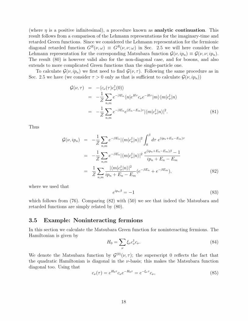
Let us first define the concept of an irreducible diagram. This is a diagram thatcannot be cut in two pieces by only cutting a single internal electron line. (The leftmostand rightmost electron lines in a diagram are called external, all other electron lines arecalled internal.) If a diagram is not irreducible it is referred to as reducible. The irreduciblediagrams in Fig. 1 are 1, 2b, 3d and 3e. All the others are reducible as they can be cut acrossan internal electron line (diagram 3a can in fact be cut in two different places). The cuttingof a reducible diagram into two pieces along a single internal electron line is illustrated fordiagram (3b) in Fig. 2.

Next we define the concept of a self-energy diagram. This is an irreducible diagramwith the two external electron lines removed. Thus from Fig. 1 one finds one self-energydiagram at first order, one at second, and two at third order. We can find a mathematicalexpression for the self-energy diagram by using the Feynman rules. It is the same as that ofthe irreducible diagram it was constructed from except that the two factors of G(0)(k) dueto the external lines are removed.

Finally, we define the self-energy Σ(k) as the sum of all self-energy diagrams (thereis an infinite number of such diagrams). Denoting the self-energy diagrams as Σ(i)(k),i = 1, 2, 3, . . ., the self-energy can be written

Σ(k) =∑

i

Σ(i)(k). (139)

28

Figure 1: Feynman diagrams for G(n)(k) for orders n = 1, 2, 3. We have indicated themomenta of the unperturbed Green functions and of the interaction lines, and the factor Nassociated with each impurity.

29

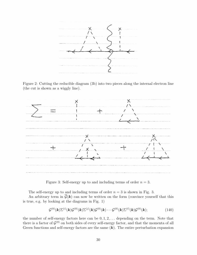
Figure 2: Cutting the reducible diagram (3b) into two pieces along the internal electron line(the cut is shown as a wiggly line).

Figure 3: Self-energy up to and including terms of order n = 3.

The self-energy up to and including terms of order n = 3 is shown in Fig. 3.An arbitrary term in G(k) can now be written on the form (convince yourself that this

is true, e.g. by looking at the diagrams in Fig. 1)

G(0)(k)Σ(i)(k)G(0)(k)Σ(j)(k)G(0)(k) · · · G(0)(k)Σ(+)(k)G(0)(k); (140)

the number of self-energy factors here can be 0, 1, 2, . . . depending on the term. Note thatthere is a factor of G(0) on both sides of every self-energy factor, and that the momenta of allGreen functions and self-energy factors are the same (k). The entire perturbation expansion

30

for G(k) can then be obtained by summing over all such terms and over all the self-energydiagrams in each term:

G(k) = G(0)(k) +∑

i

G(0)(k)Σ(i)(k)G(0)(k) +∑

i,j

G(0)(k)Σ(i)(k)G(0)(k)Σ(j)(k)G(0)(k)

+∑

i,j,k

G(0)(k)Σ(i)(k)G(0)(k)Σ(j)(k)G(0)(k)Σ(k)(k)G(0)(k) + · · ·

= G(0)(k) + G(0)(k)Σ(k)G(0)(k) + G(0)(k)Σ(k)G(0)(k)Σ(k)G(0)(k)

+ G(0)(k)Σ(k)G(0)(k)Σ(k)G(0)(k)Σ(k)G(0)(k) + · · ·= G(0)(k) + G(0)(k)Σ(k)[G(0)(k) + G(0)(k)Σ(k)G(0)(k) + · · · ]. (141)

We recognize the expression inside square brackets as the expansion of G(k) itself, so thatwe finally get

G(k) = G(0)(k) + G(0)(k)Σ(k)G(k). (142)

This is the Dyson equation. It is easily solved to give

G(k, ipm) =1

(G(0)(k, ipm))−1 − Σ(k, ipm)=

1

ipm − ξk − Σ(k, ipm), (143)

where we have reinstated the ipm variable which we dropped earlier.In general the self-energy is complex. As we will see examples of later, the real part of

the self-energy gives rise to a shift in the energy ξk, while the imaginary part gives rise to afinite lifetime.

We have no hope of finding the exact Green function, as that would require calculatingthe exact self-energy as the sum of all self-energy diagrams. However, approximating theself-energy by the sum of just a subset (finite or infinite) of all the self-energy diagrams doesgive us an approximation for the Green function through the Dyson equation. Note thateven when the number of self-energy diagrams included in this way is finite (e.g. we mayinclude just one or two terms in the self-energy; see below), it still corresponds to summingan infinite number of terms in the expansion for the Green function, as seen by iterating theDyson equation using the approximate self-energy.

4.7 Low-density weak-scattering approximation for the self-energy

We will now consider an approximation for the self-energy that is appropriate in the limit oflow impurity density nimp ≡ N/Ω and weak scattering potential U(r). In this case it sufficesto include the first two terms in the self-energy in Fig. 3. These are of first and second orderin U (as they have one and two interaction lines, respectively) and are thus the leading termsat small U (as we’ll see soon, the reason it’s necessary to include the self-energy diagramof second order in U is because the first order term is rather trivial and does not give riseto a finite lifetime). They are also of first order in the impurity density nimp because theyonly have one impurity cross; a self-energy diagram with m crosses will be of order nm

imp.Self-energy diagrams with more than one cross can therefore be neglected in the low-densitylimit.

31

To understand why each impurity cross is associated with a factor nimp, first note thatfrom the Feynman rules, a diagram of order n with m impurity crosses has n factors of U(qi)and m factors of N . Let us separate out the inverse volume 1/Ω from U(q) (see Eq. (115))by defining U(q) ≡ (1/Ω)u(q). This shows that the diagram also comes with n factors of1/Ω. Now consider the Feynman diagrams in Fig. 1. Note that a diagram of order n with mimpurity crosses contains n−m summations over internal momenta. This is valid in general,not just for the diagrams in this figure. We now associate one factor of 1/Ω with each ofthese summations over an internal momentum; this uses up n − m of these factors.9 Theremaining m factors of 1/Ω are associated with the m impurity crosses. Thus each impuritycross comes with a factor N/Ω = nimp.

Let us now evaluate the self-energy diagrams we will consider. We start with the firstdiagram in the self-energy in Fig. 3. Using the Feynman rules it is given by

Σ(1)(k, ipn) = NU(0) = nimpu(0) ≡ nimpu (144)

where we defined u(0) ≡ u. We see that in fact this diagram depends on neither k nor ipn.When inserted into the Dyson equation, it is seen to just correspond to a constant energyshift ξk → ξk + Σ(1).

The second diagram in Fig. 3 is a little more complicated. It is given by

Σ(2)(k, ipn) = N∑

k1

U(k1 − k)U(k − k1)G(0)(k1) = nimp1

Ω

∑

k1

|u(k − k1)|21

ipn − ξk1

= −nimp1

Ω

∑

k1

|u(k − k1)|2ξk1 + ipn

ξ2k1

+ p2n

. (145)

Let us for simplicity consider a very short-ranged potential U(r), so that we may to a goodapproximation neglect the momentum dependence of |u(k− k1)|2 so that this factor can betaken outside the k1 summation. Next let us introduce the density of states

D(ξ) =1

Ω

∑

k

δ(ξk − ξ). (146)

This gives

Σ(2)(k, ipn) = −nimpu2

∫ ∞

−∞dξ D(ξ)

ξ + ipn

ξ2 + p2n

. (147)

We will evaluate this integral approximately by replacing D(ξ) by its value at the Fermi levelξ = 0 where (ξ2 + p2

n)−1 is largest. In this approximation the real part of Σ(2) will vanish,since the integrand becomes odd in ξ. We thus get

Σ(2)(k, ipn) = −ipn nimpu2D(0)

∫ ∞

−∞

dξ

ξ2 + p2n︸ ︷︷ ︸

π/|pn|

= −iπpn

|pn|nimpu

2D(0) = − i

2τsgn(pn), (148)

where we have defined1

τ≡ 2π nimpu

2D(0). (149)

9Therefore each summation over an internal momentum ki can be written (1/Ω)∑

ki= 1/(2π)3

∫d3ki.

32

Inserting this into the Dyson equation gives

G(k, ipn) =1

ipn − ξk − Σ(k, ipn)=

1

ipn − ξk − nimpu + i2τ sgn(pn)

. (150)

Below we will see that the parameter τ can be interpreted as a lifetime.

4.8 The impurity-averaged retarded Green function and its spec-tral function

We now want to find the impurity-averaged retarded Green function GR(k, ω). From Sec.3.4 we know that it is given by

GR(k, ω) = G(k, ipn)|ipn→ω+iη. (151)

To do this analytic continuation we write sgn(pn) (which appears in G(k, ipn)) as a functionof ipn:

sgn(pn) = sgn(Im(ipn)). (152)

Thus the analytic continuation gives, for ω real,

sgn(Im(ipn) → sgn(Im(ω + iη)) = sgn(η) = +1, (153)

where we used that η = 0+. Thus for ω on the real axis,

GR(k, ω) =1

ω − ξk − nimpu + i2τ

. (154)

Let us now calculate GR(k, t), given by

GR(k, t) =1

2π

∫ ∞

−∞dω e−iωtGR(k, ω) =

1

2π

∫ ∞

−∞dω

e−iωt

ω − ξk − nimpu + i2τ

. (155)

We can evaluate this integral using contour integration. We note that the integrand has a polein the lower half plane at ω = ξk+nimpu− i

2τ . From the factor e−iωt = exp (−itRe ω) exp (tIm ω)we see that for t < 0 we have to close the contour in the upper half plane. The contour thenencloses no poles so that according to the residue theorem the integral is zero. On the otherhand, when t > 0 we have to close the contour in the lower half plane. Using the residuetheorem, we then pick up the residue of the pole in the lower half plane, giving

GR(k, t) =1

2π· 2πi(−1)e−i(ξk+nimpu− i

2τ )t (t > 0), (156)

here the (−1) comes from the contour being clockwise in this case. Thus we get

GR(k, t) = −iθ(t)e−i(ξk+nimpu)te−t/(2τ). (157)

Thus the retarded Green function is decaying in time; the finite lifetime comes from a nonzeroimaginary part of the self-energy. There is also a shift in the energy coming from the realpart of the self-energy.

33

We can also find the spectral function of GR(k, ω):

A(k, ω) = − 1

πIm GR(k, ω) =

1

π

1/2τ

(ω − (ξk + nimpu))2 + (1/2τ)2. (158)

This is a Lorentzian peaked at ω = ξk + nimpu and with a width proportional to τ−1. Theseresults are interpreted as follows: The free electrons are turned into “quasi-particles” by theimpurity scattering. The quasiparticles have an energy ξ∗k = ξk + nimpu and a finite lifetimeτ .

4.9 An example of linear response theory and two-particle Greenfunctions: The Kubo formula for the electrical conductivity

If an electric field of magnitude E is applied to a metal, the resulting current density J isgiven by

J = σE (159)

where σ is the conductivity. This is just a different way of writing Ohm’s law I = V/R;the resistance R is proportional to the resistivity which is the inverse of the conductivity.Eq. (159) is an example of linear response; the response (J) to the applied field (E) isproportional to the applied field; the proportionality constant (σ) is thus an example of aresponse function (cf. Sec. 1.1).

We will show that the conductivity can be expressed in terms of a retarded current-current correlation function, which is a type of two-particle retarded Green function. Theresult we will arrive at is known as the Kubo formula for the conductivity. Let us start byconsidering a system with Hamiltonian H. For now this will be taken to be unspecified; theonly thing we will assume is that it is not explicitly time-dependent. (Eventually we willtake H to be given by the impurity scattering Hamiltonian (108)). Next we assume that thissystem is being acted on by some external applied field. We assume that the coupling of thisapplied field to the system occurs through a Hamiltonian Hext which can have an explicittime dependence (which we don’t indicate in the notation) because the applied field can varywith time. Furthermore we assume that Hext is turned on “infinitely slowly”, starting attime t0 = −∞, so that at that initial time the external field was not present and the systemwas then in the ground state of H. The total Hamiltonian is then

Htot = H + Hext. (160)

The state |Ψ(t)〉 of the system evolves in time according to the time-dependent Schrodingerequation with Htot as the Hamiltonian:

i∂

∂t|Ψ(t)〉 = Htot|Ψ(t)〉, (161)

where we have set ! = 1 as usual. Let us now define

|ΨH(t)〉 = eiHt|Ψ(t)〉. (162)

34

One can show from (161) that the time evolution of |ΨH(t)〉 is given by

i∂

∂t|ΨH(t)〉 = Hext(t)|ΨH(t)〉 (163)

where we have definedHext(t) ≡ eiHtHexte

−iHt. (164)

Note that the time dependence of Hext(t) comes from two sources: the factors e±iHt in itsdefinition and the explicit time dependence of Hext itself (which we haven’t indicated in thenotation). We see from (163) that if Hext were zero, |ΨH(t)〉 would be time-independent.Eq. (163) can be integrated to give

|ΨH(t)〉 = |ΨH(−∞)〉 − i

∫ t

−∞dt′ Hext(t

′)|ΨH(t′)〉 (165)

where we have taken the initial time to be −∞, when the external field was zero and weassume that the system was in the ground state of H. We will assume that Hext is linear inthe applied field. If it also were to contain terms of higher order in the applied field, thoseterms can be neglected since we only want to find the leading, i.e. linear, response to theapplied field, which should be sufficient in the limit when the applied field is sufficiently weak.Thus it is sufficient to find |ΨH(t)〉 to linear order in Hext. Since the 2nd term on the rhs in(165) already contains a factor Hext we can therefore take Hext = 0 when evaluating |ΨH(t′)〉in that integral, which gives [from (163)] |ΨH(t′)〉 = |ΨH(−∞)〉. Defining |ΨH(−∞)〉 = |ΨH〉(the ground state of H) we thus get to linear order in Hext,

|ΨH(t)〉 = |ΨH〉 − i

∫ t

−∞dt′ Hext(t

′)|ΨH〉. (166)

Now let us find an expression for the expectation value of an operator o(r) in the state|Ψ(t)〉,

O(r, t) ≡ 〈Ψ(t)|o(r)|Ψ(t)〉 = 〈ΨH(t)|eiHto(r)e−iHt|ΨH(t)〉 = 〈ΨH(t)|o(r, t)|ΨH(t)〉. (167)

Again, we just want the linear response, so inserting (166) and keeping only terms that arefirst order in Hext gives

O(r, t) = 〈o(r, t)〉 − i

∫ t

−∞dt′ 〈[o(r, t), Hext(t

′)]〉 (168)

where all the expectation values on the rhs are with respect to |ΨH〉, the ground state of H.This is an important point: The linear response is determined by an expectation value withrespect to the unperturbed system (i.e. the system in the absence of the external appliedfield). This is as far as we can get on general grounds. To make further progress we mustspecify what o(r) and Hext are.

We will take o(r) to be a component of the current operator10 j(r) and Hext to be theHamiltonian describing how an electric field couples to the system to linear order. Let us

10Strictly speaking we mean the current density operator, but for simplicity we will refer to it as thecurrent operator.

35

first consider the current operator. For a system of “classical” electrons it would be givenby

j(r) =e

m

Ne∑

i=1

(pi − eA(ri))δ(r − ri). (169)

Here e is the electron charge (i.e. e = −|e| < 0), m is the electron mass, ri and pi are theposition and momentum of the i’th electron, and A is the vector potential. We are interestedin the current response to an electric field E which can be expressed in terms of the vectorpotential as E = −∂A/∂t. The scalar electromagnetic potential φ is not needed and can beset to zero.

In “first quantization” the current operator can be written

j(r) = jP (r) + jD(r) (170)

where

jP (r) =e

2m

∑

i

[piδ(r − ri) + δ(r − ri)pi], (171)

jD(r) = −e2

m

∑

i

A(ri)δ(r − ri). (172)

Here we have separated the current operator into a “paramagnetic” and “diamagnetic” part(this could have been done already in the classical expression above). In these expressions ri

and pi are quantum-mechanical operators (ri → ri, pi → −i∇i). Since they don’t commutetheir order matters. This is why in jP (r) they appear in a symmetrized way; this is necessaryfor jP (r) to be a Hermitian operator.

In “second quantization” these current operators can be shown to be given by

jP (r) = − ie

2m

∑

σ

(ψ†

σ(r)∇ψσ(r)− [∇ψ†σ(r)]ψσ(r)

), (173)

jD(r) = −e2

mA(r)

∑

σ

ψ†σ(r)ψσ(r), (174)

where ψ†σ(r) and ψσ(r) respectively create and annihilate an electron with spin projection

σ at position r.Next let us consider how the vector potential enters the Hamiltonian. This happens

through the term ∑

i

1

2m(pi − eA(ri))

2. (175)

This form is valid in both classical mechanics and quantum mechanics, if one interprets ri

and pi appropriately (i.e. as operators in the latter case). In second quantization this termbecomes

1

2m

∑

σ

∫dr ψ†

σ(r)(−i∇− eA(r))2ψσ(r). (176)

36

From this Hext can be extracted as the part that is linear in A. This gives

Hext = −∫

drjP (r) · A(r) = −∫

dr∑

β=x,y,z

jPβ (r)Aβ(r). (177)

Now we take o(r) = jα(r) in (168) where α = x, y, or z. Inserting our expressions forthe current operators and Hext gives

Jα(r, t) = 〈jα(r, t)〉 − i

∫ t

−∞dt′ 〈[jα(r, t),−

∫dr′

∑

β=x,y,z

jPβ (r′, t′)Aβ(r′, t′)]〉. (178)

Here we have also introduced the explicit time dependence of A (which we haven’t indicatedearlier in order not to clutter the notation). However, this is not yet the linear response result.First of all, since the commutator already contains an explicit factor of A, we can omit thediamagnetic part of jα(r, t) since it would lead to a contribution that is quadratic in A.Thus we can replace jα(r, t) → jP

α (r, t) in the commutator. Second, 〈jα(r, t)〉 = 〈jDα (r, t)〉

since 〈jPα (r, t)〉 = 0 (because there is no current in the absence of an electric field). We also

use that〈∑

σ

ψ†(r, t)ψσ(r, t)〉 = n(r), (179)

where n(r) is the electron density at the point r (the expectation value is time-independentsince H is time-independent). Furthermore, we can extend the upper limit in the t′ integra-tion to ∞ by introducing a factor θ(t− t′) into the integrand. This gives

Jα(r, t) = −∑

β

∫ ∞

−∞dt′

∫dr′ ΠR

αβ(r, r′; t− t′)Aβ(r′, t′)− e2

mn(r)Aα(r, t), (180)

where we have introduced the retarded current-current correlation function

ΠRαβ(r, r′; t− t′) = −iθ(t− t′)〈[jP

α (r, t), jPβ (r′, t′]〉. (181)

As indicated this correlation function depends only on the time difference t − t′ since H istime-independent. We now take the time Fourier transform of (180). The Fourier transformof the time convolution is the product of the Fourier transforms of each factor, giving

Jα(r, ω) = −∑

β

∫dr′ ΠR

αβ(r, r′; ω)Aβ(r′, ω)− e2

mn(r)Aα(r, ω). (182)

Next, from E(r, t) = −∂A(r, t)/∂t we get, for A(r, t) = A(r, ω)e−iωt + c.c.,

E(r, t) = − ∂

∂t(A(r, ω)e−iωt + c.c.) = −(−iωA(r, ω)e−iωt + c.c.) ≡ E(r, ω)e−iωt + c.c.

⇒ E(r, ω) = iωA(r, ω). (183)

Using this in (182) we can write

Jα(r, ω) =∑

β

i

ω

[∫dr′ ΠR

αβ(r, r′; ω)Eβ(r′, ω) +e2

mn(r)δαβEβ(r, ω)

]. (184)

37

Finally, if we average over the impurity positions the system becomes translationally invari-ant, and therefore

ΠR(r, r′; ω) → ΠR(r, r′; ω) = ΠR(r − r′, ω), (185)

n(r) → n(r) = n, (186)

where n = Ne/Ω is the overall electron density. If we now do a space Fourier transformof (184), using that the Fourier transform of a convolution in space is the product of theFourier transforms of each factor, we get

Jα(q, ω) =∑

β

σαβ(q, ω)Eβ(q, ω), (187)

where the conductivity tensor is given by

σαβ(q, ω) =i

ω

[ΠR

αβ(q, ω) +ne2

mδαβ

]. (188)

This is our final result for the conductivity, the Kubo formula.

4.10 Calculating the conductivity from the Kubo formula

Main steps involved in the calculation of the conductivity:

1. Define an imaginary-time (Matsubara) analogue to the retarded current-current cor-relation function:

παβ(r1, r′1; τ1 − τ ′1) = −〈Tτ (j

Pα (r1, τ1)j

Pβ (r′1, τ

′1))〉. (189)

This is easier to calculate than the retarded function. Note that this Matsubara func-tion is bosonic in the sense that it is periodic, not anti-periodic, when the time argu-ment is translated by β. This is related to the fact that each current operator containsan even number (two) of fermionic operators. To get the retarded function from theimaginary-time function, one follows the conventional recipe of analytic continuationof the end result: iωn → ω + iη.

2. The function (189) can be expressed as

παβ(r1, r′1; τ1 − τ ′1) =

e2

4m2

∑

σσ′

(∇2′β −∇1′β)(∇2α −∇1α)

〈Tτ (ψσ(r2, τ2)ψσ′(r′2, τ

′2)ψ

†σ′(r

′1, τ

′1)ψ

†σ(r1, τ1))〉τ ′2=τ−1 , r′2=r1

τ2=τ−1 ,r2=r1

, (190)

where the time-ordered expression appearing here is a two-particle Matsubara Greenfunction. To arrive at this result we have used that fermionic field operators thatare all under a time-ordering symbol can be moved around freely if one introduces aminus sign every time two such field operators pass each other. (In this expression thederivatives act before the 2-coordinates are set equal to the 1-coordinates.)

38

3. Next, an important theorem called Wick’s theorem can be used to express the time-ordered two-particle Green function in this expression as a sum of products of twotime-ordered single-particle Green functions:

〈Tτ (ψσ(r2, τ2)ψσ′(r′2, τ

′2)ψ

†σ′(r

′1, τ

′1)ψ

†σ(r1, τ1))〉

= 〈Tτ (ψσ(r2, τ2)ψ†σ(r1, τ1))〉〈Tτ (ψσ′(r

′2, τ

′2)ψ

†σ′(r

′1, τ

′1))〉

− 〈Tτ (ψσ(r2, τ2)ψ†σ′(r

′1, τ

′1))〉〈Tτ (ψσ′(r

′2, τ

′2)ψ

†σ(r1, τ1))〉

= Gσσ(r2, τ2; r1, τ1)Gσ′σ′(r′2, τ

′2; r

′1, τ

′1)− Gσσ′(r2, τ2; r

′1, τ

′1)Gσ′σ(r′2, τ

′2; r1, τ1).(191)

This is a very significant simplification. Wick’s theorem is valid when the expectationvalues are with respect to a Hamiltonian that is quadratic in fermion operators, as it ishere. According to Wick’s theorem, to arrive at this expression one pairs up creationoperators with annihilation operators in all possible ways. The paired operators arethen moved so they appear next to each other. In this process a minus sign is introducedevery time two fermion operators are moved past each other. Thus the product of thesesigns gives the overall sign in front of the term. Next, the expectation value in eachterm factorizes into products of single-particle Green functions. Since we here havetwo creation and two annihilation operators, there are two different ways to pair them,which is why we get two terms in the sum on the rhs.

4. The first term in this expression gives, when substituted into (190), an expressioninvolving 〈jP

α (r1, τ1)〉〈jPβ (r′1, τ

′1)〉. This is zero because there is no current in the ab-

sence of an electric field. So only the second term in the pairing contributes to theconductivity.

5. We now Fourier transform to wavevector and Matsubara frequency space. Since wehave reduced the problem to one involving a product of two single-particle Greenfunctions, we can use the perturbation expansion we developed for this function inSec. 4.3. Thus this product has a perturbation expansion given by the product of theperturbation expansions for each of the two single-particle Green functions.

6. We would like to find the conductivity σαα(q = 0, ω = 0) ≡ σ, i.e. the response toan electric field that is uniform in space and constant in time, for a system that isisotropic in space. We can set q = 0 directly. However, because ω appears in thedenominator in (188) we cannot set ω = 0 directly. Instead we have to look at finiteω and take the limit ω → 0. This is however what we would have done anyway, sincewe first have to calculate the Matsubara function for an arbitrary iωn and then do theanalytic continuation iωn → ω + iη.

7. Next we do the impurity averaging. As for the single-particle Green function consideredearlier, each term in the resulting expansion for παα(q = 0, iωn) ≡ π(iωn) can berepresented by a Feynman diagram. These will however look different from the onesfor the single-particle Green function and will have different Feynman rules. Thesimplest diagram in this expansion is shown in Fig. 4(a) (it doesn’t have any impurityscatterings). The upper and lower electron lines form a loop (“biting each other’stail”). There is conservation of momentum at each of the two vertices where the two

39

electron lines meet (shown as black dots). There is also conservation of the Matsubarafrequency at each of these vertices. Note however that there is an external (bosonic)frequency iωn at each of these two vertices which makes the (fermionic) Matsubarafrequencies of the two electron lines differ by ωn. The internal fermionic Matsubarafrequency ipn goes in a loop and so is undetermined by frequency conservation. Hencethere is a sum over ipn.

8. The impurity averaging leads to two different classes of diagrams. Some examplesof diagrams in the first class are shown in Fig. 4(b). In this class of diagrams, anygiven impurity in the diagram (represented by an impurity cross) scatters only withthe upper line or only with the lower line. So any such diagram therefore contains aproduct of two Green function diagrams of the type we have seen before. All thesediagrams can be summed exactly; the result is just given in terms of the product ofthe full Green functions for the upper and lower line. The mathematical expression forthis sum is

2e2

3m2Ω

∑

k

k2 1

β

∑

ipn

G(k, ipn + iωn)G(k, ipn). (192)

Thus note that the Green functions in this expression are the full Green functions, notthe unperturbed (G(0)) ones. The diagrammatic representation of this term is givenin Fig. 4(c). The electron lines are drawn thick to indicate that they represent thefull Green function. For obvious reasons this diagram is frequently referred to as “thebubble diagram”.

9. In the second class of diagrams, there are impurities which scatter with both lines.These diagrams contain dashed interaction lines that straddle (via an impurity) boththe upper and lower electron lines. Some examples of such diagrams are shown inFig. 4(d). The set of these diagrams is referred to as vertex corrections. The typesof vertex correction diagrams that can appear are dictated by our approximation forthe self-energy. It turns out that for the approximation for the self-energy we used,which gave a momentum-independent self-energy, these vertex corrections cancel forthe q = 0 conductivity we want to calculate. So it is sufficient to calculate only thebubble diagram. This is no longer true when using a more accurate, momentum-dependent, approximation for the self-energy, however.

10. The calculation of the bubble diagram is rather involved in itself, but won’t be describedin any detail here. The end result (after doing the analytic continuation) is that wefind a conductivity given by

σ =ne2τ

m(193)

where n is the electron density and τ is the lifetime defined in (149). This is of thesame form that one gets from simple (classical) Drude theory.

40

5 Concluding remarks

Although in these introductory notes we have only had time to discuss one application ofthe Green function formalism, namely to electrons in a disordered potential, it is importantto note that concepts and results like Feynman diagrams, the self-energy, and the Dysonequation, continue to be valid and central in applications of this formalism to other problemsas well. For example, if one considers the problem of interacting electrons, and develops aperturbation expansion for the single-particle Green function of this problem, each term inthe perturbation expansion can again be represented as a Feynman diagram. Although theappearance of these diagrams, and the Feynman rules, will be different from those of theimpurity scattering problem, one can again define irreducible diagrams in exactly the sameway (i.e. as Feynman diagrams that cannot be cut into two separate pieces by only cuttinga single internal electron line) and from those one defines self-energy diagrams and then theself-energy as the sum of all self-energy diagrams. Furthermore, the Dyson equation relatingthe single-particle Green function and the self-energy continues to hold.

41