l copy - nasa 3 - perturbation methods ..... 32 3.1 methods of adjqint functions 36 3.2 methods of...
TRANSCRIPT

t
NASA TECHNICAL MEMORANDUM NASA TM X-58065November 1971
AN ANALYSIS AND COMPARISON OF SEVERAL*
TRAJECTORY OPTIMIZATION METHODS
COPYL
NATIONAL AERONAUTICS AND SPACE ADMINISTRATION
MANNED SPACECRAFT CENTER
HOUSTON, TEXAS 77058
https://ntrs.nasa.gov/search.jsp?R=19720006176 2018-06-17T05:37:07+00:00Z

NASA TM X-58065
AN ANALYSIS AND COMPARISON OF SEVERAL
TRAJECTORY OPTIMIZATION METHODS
J. M. LewallenManned Spacecraft Center
Houston, Texas

PREFACE
/" • ' : ' • ' . • ' -
The optimization and control of spacecraft trajectories
has been of considerable interest during the past decade, and a
significant amount of progress has been made in developing a
theoretical and numerical capability to solve complex trajec-
tory problems. There still exists, however, a need to deter-
mine the best approach, given a specific problem. The gener-
ality of such a task is overwhelming, but an Initial step is
taken when most of the promising methods have been studied
with the aid of a specific, but representative example. This
dissertation takes this first step, and along with several
significant theoretical and numerical contributions, compares
the relative merits of several trajectory optimization methods.
In each stage of this research, the author has bene-
fited from many valuable suggestions by and discussions with
many individuals. He wishes to express sincere appreciation to
W. T. Fowler, G. J. Lastman, and J. F. Jordan who, as fellow
students, provided considerable encouragement. He wishes to
express gratitude to Professors L. Clark, W. Carter and
E. Prouse of The University of Texas for reading the manuscript
and making helpful suggestions. The author is especially in-
debted to R. D. Witty of the Lockheed Electronic Corporation,
without whose patience, intelligence and persistence the en-
deavor, as presented, would have never been realized.
iii

The author also wishes to express gratitude to
E. L. Davis, Jr. of the Manned Spacecraft Center for provid-
ing a stimulating environment and great encouragement during
the course of this study. He is especially indebted to
,rofessor B. D. Tapley of The University of Texas who served
as advisor, but more than that a good friend and teacher and
a constant source of inspiration and guidance.
The author wishes to express his deepest gratitude to
his wife and children, whose love and patience made -the wholeVi
undertaking worth doing.
Houston, Texas Jay M. Lewallen
May 1966
iv
ABSTRACT
A theoretical development and comparative evaluation is
made for several methods of solving the problem associated with
the optimum transfer of a spacecraft. Particular attention is
given to the sensitivity of the convergence characteristics of
the methods to initially assumed parameters and trial solutions,
convergence times, .computer logic and storage requirements.' '
The methods considered may be classified as one of the
following types: (1) Perturbation, Second Variation or Ex-
tremal Field Methods, (2) Quasilinearization or Generalized
Newton-Raphson Methods, or (3) Gradient or Steepest Descent\
Methods. The numerical comparison of the convergence, charac-
teristics is made by considering a minimum time, low thrust,V
Earth-Mars transfer trajectory.
A new quasllinearization method, called the Modified
Quasilinearization Method, is proposed. For the example con-
sidered, this method reduces convergence time by approximately
7Q% when compared with the Generalized Newton-Raphson Method.
Moreover, the method allows the terminal boundary to be speci-
fied by a general function of the problem variables rather
than individual values of the variables themselves.
A uniquely specified and easily determined, time de-
pendent weighting matrix has been discovered for the gradient
techniques. This weighting matrix accelerates the shaping of

the optimal control program and Improves the convergence
characteristics during the terminal iterations by giving more
weight to regions of low sensitivity.
Convergence envelopes, which give an indication of how
sensitive the convergence characteristics are to initially
assumed parameters, are plotted for the Perturbation and
Quasillnearization Methods. Several iteration schemes are
proposed which significantly increase the size of the con-
vergence envelopes, and hence decrease the sensitivity of
the method to initially assumed parameters.
vi

TABLE OP CONTENTS '-
i. ,Page
PREFACE Hi
ABSTRACT ,. . . ' . . - . v
LIST OF FIGURES • - . . . ' • x
LIST OF SYMBOLS . . .., xv
CHAPTER 1 - INTRODUCTION • - . . . . - . . . . ' 1
1.1 Definition of the Optimization Problem 1
1.2 Background Study of Optimization Theory . . . . 3
1.3 Purpose of the Investigation . . . . . " 14
1.4 Scope of the Investigation 14
CHAPTER 2 - FORMULATION OF THE OPTIMIZATION PROBLEM ... 16
2.1 Derivation of the Necessary Conditions for anOptimal Trajectory i 16
2.2 Reduction of the Optimization Problem to a Two-Point Boundary Value Problem 24
CHAPTER 3 - PERTURBATION METHODS . . . . . . . 32
3.1 Methods of Adjqint Functions 36
3.2 Methods of Perturbation Functions . . . . . . . 45
3.3 Iteration Philosophy for the PerturbationMethods 51
CHAPTER 4 - QUASILINEARIZATION METHODS . . .' '59
4.1 Methods of Generalized Newton-Raphson £0
4.2 Modified Quasilinearization Method 66
4.3 Iteration Philosophy for the QuasilinearizationMethods ." 70
vii

TABLE OF CONTENTS .
(CONT'D)
- Page
CHAPTER 5 - GRADIENT METHODS . . . .......... . 75
5.1 Method of Steepest Descent ....... . . . 76
5.2 Modified Method of Steepest Descent . . . . . . 84
5.3 Iteration Philosophy for the Gradient Methods . 89
CHAPTER 6 - COMPARISON AND DISCUSSION OF THE OPTIMIZA-TION METHODS AND ITERATION SCHEMES ..... 100
6.1 Selection of Methods for Comparative Study . .
6.2 Basis of Comparison .............. . 1°2
6.3 Perturbation Methods .......... . . . 103
6.4 Quasilinearization Methods .......... .1^
6.5 Gradient Methods ........ . . . . . . . 165
6.6 Summary of the Comparison . . . . . . . . . . . "178
CHAPTER 7 - DESCRIPTION AND EVALUATION OF NUMERICAL . .PERFORMANCE ........... . . . . . . . 180
7.1 Numerical Integration . . . . . ....... .
7.2 Linear System Routine ............ .
7.3 Numerical Criteria Affecting Accuracy . . . . .
7.4 Computation Facilities ........ . . . .
CHAPTER 8 - CONCLUSIONS AND RECOMMENDATIONS . . .....
8.1 Summary of Conclusions . . . . ........
8.2 Recommendations for Continued Study ..... .
APPENDICES .................... ... 196
viii

TABLE OP CONTENTS
(CONT'D)
Page
A.I Application of the Reduction of an OptimizationProblem to a Two-Point Boundary Value Problem . . 196
A. 2 Discussion of the Applications . ........ 202
A. 2.1 Application of the Method of Adjoint Func-tions .............. . . . . 211
A. 2. 2 Application of the Method of PerturbationFunctions . . . . . ...... . . . . . ?!'<
A. 2. 3 Application of the Modified Quasilineariza-tion Method ..... ... ....... v. • 217
A. 2.^ Application of the Method of SteepestDescent .................
A. 2. 5 Application of the Modified Method ofSteepest Descent
A. 3 Numerical Constants . . . . . . ........... ??"!t
A. 4 Normalization Scheme . . . . . . . . . . . . . . ?-r)
BIBLIOGRAPHY . . . . .......... . . . ..... ?30
VITA ..... . . . . .......... . . . . . . 233
ix

LIST OF FIGURES
Figure Pagei
1 Convergence Envelope for the MAF Using theNormal Iteration Scheme, Initial IterationFactor of 100% and Terminal Time Error of-20% . . ............ ...... . . 107
/
2 'Convergence Envelope for the MAF Using theNormal Iteration Scheme, Initial Iteration • •J-'nctnr of 100/5 and Terminal Time Error ofu> . • ........... .......... 108
3 Convergence Envelope for the MAF Using theNormal Iteration Scheme, Initial IterationFactor of 100% and Terminal Time Error of20% ................. / ' ' ' 109
lJ Convergence Envelope for the MAF Using It-eration Scheme 1, Initial Iteration Factorof 100% and Terminal .Time Error of -20% • • • 112
5 Convergence Envelope for the MAF Using It-eration- Scheme. 1, Initial Iteration Factorof 100% and Terminal Time Error of 0% . . • • H3
6 Convergence Envelope for the MAF Using It-eration Scheme 1, Initial Iteration Factorof 100% and Terminal Time Error of 20% . . . . H4
7 Convergence Envelope for the MAF Using It- :eration Scheme 1, Initial Iteration Factorof 50% and Terminal Time Error of -20% • • • • 1:L5
8 Convergence Envelope for the MAF Using It-eration Schemes 1 and 2, Initial IterationFactor of 50%, Terminal Time Error of 0%and Update Integer of 1 ...... - ..... Ho
9 Convergence Envelope for the MAF Using It-eration Scheme 1, Initial Iteration Factorof 50% and Terminal Time Error of 20% . . . . 117
10 Convergence Envelope for the MAF Using It-eration Scheme 2, Initial Iteration Factorof 50%, Terminal Time Error of 0% and Up-date Integer of 2 ........... ... 119

Figure Page
11 Convergence Envelope for the MAP Using It-eration Scheme 2, Initial Iteration Factorof 5055, Terminal Time Error of Q% and Up-date Integer of ^ 120
12 Convergence Envelope for the MAF Using It-eration Scheme 2, Initial iteration Factorof 5055, Terminal Time Error of 0/J and Up-date Integer of 6 . . . . . . . 121
13 - Convergence Time as a Function of the InitialValue of Iteration Factor for the MAF UsingIteration Scheme 1 123
14 Convergence Time as a Function of the InitialValue of Iteration Factor for the MAF UsingIteration Scheme 2 125
15 Convergence Envelope for the MAF Using It-eration Schemes 1 and 2, Initial IterationFactor of 50/S, Terminal Time Error of 0/Jand Update Integer of 1 (Time) • 126
16 Convergence Envelope for the MAF Using It-eration Scheme 2, Initial Iteration Factorof 50#, Terminal Time Error of 0% and Up-date Integer of 2 (Time) • 127
17 Convergence Envelope for the MAF Using It-eration Scheme 2, Initial Iteration Factor
• of 50%, Terminal Time Error of 0/J and Up-date Integer of 4 (Time) 128
18 Convergence Envelope for the MAF Using It-eration Scheme 2, Initial Iteration Factorof 50%, Terminal Time Error of Q% and Up-date Integer of 6 (Time) .' . . 129
19 Norm of Terminal Constraints as a Functionof Computation Time for the MAF Using It-eration Scheme 1 • • • • 131
20 Norm of Terminal Constraints as a Functionof Computation Time for the MAF Using It-eration Scheme 2 • 132
xi

Figure Page
21 Convergence Envelope for the MAP Using theNormal Iteration Scheme, Initial IterationFactor of 1005? and Terminal Time Error of-1055 (Earth Launch) . ........... . . 13'l
22 Convergence Envelope for the MAP Using theNormal Iteration Scheme", Initial IterationFactor of 100$ and Terminal Time Error of0% (Earth Launch) . ... . . - . . , . . . . . . 135
23 Convergence Envelope for the MAP Using theNormal Iteration Scheme, Initial IterationFactor of 100$ and Terminal Time Error .of10$ (Earth Launch) ........ ..... . 136
2U Convergence Envelope for the MPF Using It-eration Scheme 1, Initial Iteration Factorof 100$ and Terminal Time Error of 0$ . . . . . 1^0
25 Convergence Envelope for the MPF Using Alt-eration Scheme 1, Initial Iteration Factorof 50$ and Terminal Time Error of 0$ ... ... . I'll
26 Convergence Envelope for the MPF Using It-eration Scheme 1, Initial Iteration Factorof 100$ and Terminal Time Error of 0$ (Time) , . 1*»2
27 "Convergence Envelope for the MPF Using It-eration Scheme 1, Initial Iteration Factorof 50$ and Terminal Time Error of 0$ (Time) . . 1^3
' i
28 Metric p as a Function of Computation Time.for the MGNR Using the Normal Iteration Scheme . 1^8
29 Metric p .as a Function of Convergence Timefor the MGNR Using Iteration Scheme 1 ,Initial Iteration Factor of 100$ and aLinear Initial Solution . . . . . . ...... 1^9
30 Metric p as a Function of Computation Timefor the MMGNR Using the Normal IterationScheme . ............ ..... . • • 151
31 Convergence Envelope for the MQM Using the .Normal. Iteration Scheme, Initial IterationFactor of 100$ and Terminal Time Error of-20$ .................... 154
xii

Figure . : Page
32 Convergence Envelope for the MQM Using theNormal Iteration Scheme, Initial IterationFactor of 1005? and Terminal Time Error of0%. . . . . . . . . . . . . . . . . . . . . . 155
33 Convergence Envelope for the MQM Using theNormal Iteration Scheme, Initial IterationFactor. of 100$ and Terminal Time Error of2Q% ..... . • . ........ ..... 156
34 Convergence Envelope for the MQM Using It-eration Scheme 2, Initial Iteration Factorof 50% and Terminal Time Error of -2055 ^y
35 Convergence Envelope for the MQM. Using It-eration Scheme 2, Initial Iteration Factorof 505? and Terminal Time Error of Q% ..... 158
36 Convergence Envelope for the MQM Using it-eration Scheme 2, Initial Iteration Factorof 50$ and Terminal Time Error of 20$ . . . 159
37 Convergence Envelope for the MQM Using It-eration Scheme 2, Initial Iteration Factorof 5055 and Terminal Time Error of 0% (Time) • l6l
38 Metric p as a Function of ComputationTime for the MQM Using Iteration Scheme 2,Initial Iteration Factor of 100% and forLinear and Nonlinear Initial Solutions • • • 162
39 Convergence Time as a Function of theInitial Value of Iteration Factor for theMQM Using Iteration Scheme 2 and a Non-linear Initial Solution ..........
40 - Metric p as a Function of ComputationTime for the MQM Using Iteration Scheme 2and a Nonlinear Initial Solution . ...... 166
41 Thrust Angle as a Function of Mission Timefor Earth-Mars Transfer Using the MSD andWeighting Matrix W « I (Case 1) ...... 171
42 Thrust Angle as a Function of Mission Timefor Earth-Mars Transfer Using the MSD andWeighting Matrix W - I (Case 2) . . . . . . 172
xiii

Figure Page
43 Thrust Angle as a Function of Mission Timefor Earth-Mars Transfer Using the MSD andWeighting Matrix W - HUU (Case 1) ...... 173
l\i\ Thrust Angle as a Function of Mission Time .for Earth-Mars Transfer Using the MSD andWeighting Matrix W - HUU (Case 2) . :.. . . .'. 17*1
45 Convergence Time as a Function of Integra-tion Step Size Using Normal Iteration
A. 2.1
A. 2. 2
A. 2. 3
A. 2.1
Optimal Trajectory for the Earth-Mars Trans-
Optimal Constant and Unbounded Thrust Pro-
Optimal Trajectory for the Atmospheric
Optimal Constant and Unbounded Thrust Pro-
185
205
207
208
gram for the Atmospheric Earth Launch .... 210
xiv

LIST OF SYMBOL?
The following list tabulates all significant symbols
used in the main text. Each symbol is accompanied by a brief
description and the equation number where the symbol is first
introduced. A definition of'each symbol is given where the
symbol is introduced.
Matrices;
The matrix size is Indicated in the statement immedi-
ately following the symbol. The following specific indices
are used.
n - the number of state variables,
m - the number of control variables
p - the number of initially specified con- ,straint relations .
q - the number of terminally specified con-straint relations
A 2n x 2n matrix of partial derivatives, (3.2)
P n x n matrix of partial derivatives, (5.5)
G n x m matrix of partial derivatives, (5-5)
I 2n x 2n unity matrix, (3.10)
W m x m matrix of arbitrary weighting terms, (5.19)
xv

LIST OF SYMBOLS
. .(CONT'.D)
Y 2n x 2n-p matrix of homogeneous, solutions, (4.6)
j0 2n x 2n matrix of partial derivatives resulting, fromthe 2n backward integrations of the 2n vector ofadjoint equations, (3.10)
20 2n x 2n matrix of partial derivatives resulting fromthe 2n forward integrations of the 2n vector ofadjoint equations, (3.1*0
•O n+1 x 2n matrix of partial derivatives resulting from
the ri+1 backward integrations of the 2n vector ofadjoint equations, (^ .15) .
0 n+1 x 2n matrix of partial derivatives resulting fromthe n+1 backward integrations of the 2n vector ofadjoint equations, (3-17)
* 2n x 2n matrix of partial derivatives resulting from1 the 2n forward integrations of 'the 2n vector of
perturbation equations, (3.22) .
* n+1 x 2n matrix of partial derivatives resulting from2 the n+1 forward integrations of the ' 2n vector of
perturbation equations, (3.27)
* 2n x n matrix of partial derivatives resulting fromthe n forward integrations of the 2n vector ofperturbation equations, (3.29)
Vectors:
All vectors are column vectors unless otherwise noted.
The vector size is Indicated in the statement immediately fol-
lowing the symbol, where the indices are defined in the pre-
vious section on matrices.
xvi

LIST OF SYMBOLS-•>
(CONT'D)
B 2n vector of nonhomogeneous terms, (4.3)
c n+1 vector of desired percentage corrections in theterminal constraints, (3-31)
C 2n-p vector of corrections required for the assumedinitial conditions, (4.6)
f n vector of state variable derivatives, (2.1)
P 2n vector of state and Euler-Lagrange variable de- .rivatives, (2.37)
g n vector of initial constraint relations, (2.40)
h n+1 or q+n+1 vector of terminal constraint rela-tions, (2.32)
dh n+1 or q+n+1 vector of terminal dissatisfactionchange, (3-4)
u m vector of control variables, (2.1)
w 2n vector of nonhomogeneous solutions (4.5)
x n vector of state variables, (2.1)
y 2n vector of homogeneous solutions, (4.4)
2 2n vector of state variables and Euler-Lagrangevariables, (2.37)
dfi q+1 vector defined as d> - Uyn«*)0 > (5.29)
n p vector of specified initial constraint relations,'(2.3) ' .
X n vector of time dependent Lagrange multipliers,(2.5)
A 2n vector of adjoint variables, (3-3)
v q vector of constant Lagrange multipliers, (2.5)
V q vector of specified terminal constraint relations,(2.4)
xvil

LIST OP SYMBOLS
(CONT'D)
Scalars:
a constant that represents the terminal value of time.(1.9)
>,
E Weierstrass E-Function, (5-50)
CM universal gravitational constant; (A.1.1)m
H generalized Hamiltonian equal to X f, (2.6)
I auxiliary functional to be extremized, (2.5)
K step size in gradient space, (5. 6)
m instantaneous spacecraft mass, (A.1.1)TP auxiliary functional equal to <|> + v Y, and penalty
function, (5.35)
r instantaneous radial position, (A.1.1)
s Independent variable where t = as, M.9)
dS step size in control space, (5.19)
t independent variable, time, (2.1)
T thrust, (A.1.1)
u instantaneous radial velocity, (A.1.1)
v instantaneous tangential velocity, (A.1.1)
W. weighting constants where 1 = 0,q, (5-35)
u constant Lagrange multiplier, (5.24)
p metric defined in Eq. (4.7)
$ performance index, (2.2)
n stopping condition, (5-^)
xviii

LIST OF SYMBOLS
(CONT'D)
Superscripts:
(') differentiation with respect to timem . - - . . . ' ' ' '
( ) matrix transpose
( ) first variation or first derivative with respect tos
( ) second variation
( )~ matrix- inverse
( ) refers to an optimal trajectory
(~~) refers to an assumed value
Subscripts;
( ) specified initial valueo
( )f specified terminal value
( ) . partial derivative of the subscripted quantity*•» » ' with respect to x, u, x, t, respectively
( ) n trajectory iteration
( ) kth time iteration
( ) Earthe( •) Marsm( ) Suns
Uscellaneous Symbols;
d total variation or differential operator, i.e.
d( )•«()+(') dt
xlx

LIST OP SYMBOLS
(CONT'D)
6 variation operator
X(tf) evaluation of the Instantaneous variable X attime t^ .
Abbreviations:
MAP Method of Adjoint Functions
MPF Method of Perturbation Functions
MGNR Method of Generalized Newton-Raphson
MMGNR Modified Method of Generalized Newton-Raphson
MQM Modified Quasilinearization Method
MSD Method of Steepest Descent
MMSD Modified Method of Steepest Descent .
AU Astronomical Unit
XX

CHAPTER I
INTRODUCTION
A treatise on the theory of trajectory optimization and
its application requi-res a clear and meaningful definition of the
problem. This definition should include a discussion of the
terms and concepts required in studying the background material
and the theoretical formulations. An indication of the purpose
of the investigation is given along with the extent or scope of
such a study.
1.1 Definition of the Optimization Problem
The optimization of spacecraft trajectories has been of
considerable interest for a number of years, and significant pro-
gress has been made in developing a capability for solving very
complex trajectory problems. In one class of optimization prob-
lems, it is desired to determine the history of the control vari-
ables in such a manner that certain specified initial and termi-
nal constraints are satisfied while some performance index is ex-
tremized. The control variables are unspecified inputs to t'r.e
system which may be chosen to control the state, i.e., the posi-
tion and velocity. The initial and terminal constraints are
simply conditions on the position and velocity that must be sat-
isfied at the initial and terminal time, respectively. The per-
formance index is usually a scalar function associated with the
spacecraft performance and is the quantity to be extremized. It
may be a scalar function of the terminal state and time and/or a
scalar integral term evaluated along the trajectory.
The calculus of variations is the classical tool for
solving such problems, and with its use necessary conditions for
an optimal trajectory may be derived. These necessary conditions
are derived in Chapter 2 and consist of boundary conditions re-
ferred to as transversality conditions, algebraic equations re-
ferred to as optlmality conditions and the Euler-Lagrange dif-
ferential equations. The optimality conditions and the Euler-
Lagrange equations must be satisfied at each point in the time
interval of interest. A closed form solution for these equations
and boundary conditions is very difficult to obtain and has been
obtained for only a few relatively simple cases. When an optimi-
zation problem is solved numerically in such a way that the ne-
cessary conditions are satisfied, the method is usually desig-
nated an indirect method.
•There have been alternate methods developed to solve the
above stated class of problems without using the necessary condi-
tions derived with the calculus of variations. These methods,
usually referred to as direct methods, use influence functions
which indicate how the performance index and terminal constraints
are influenced by initial state variations and integrated control
variations. .
In both the indirect and direct methods, the terminal
constraints are handled in either the so-called "hard" or "soft"-v
forms. In the "hard" form an effort is made to satisfy the
terminal constraints identically while in the "soft" form the

terminal constraints are satisfied only approximately. It is
with this latter case that the penalty function concept to be
..discussed later is introduced. The philosophy used in this
method is that a certain penalty is accepted because of the
approximate satisfaction of the terminal constraints.x /
1.2 Background Study of Optimization Theory
In assessing the "state of the art" in trajectory optimi-
zation theory and application, it is helpful to understand the
developments that lead to this current state. This background is
divided into-previous and recent developments, the recent devel-
opments being made since about I960. The distinction between in-
direct and direct methods has become increasingly clear during
these recent years and are discussed separately.
1.2.1 Previous Developments .I
The original trajectory optimization problems were formu-
lated in terms of a set of nonlinear, ordinary differential equa-
tions, which were required to satisfy split boundary conditions.
The first problems to be solved were extremely simple since
numerical solution of the more difficult problems required ex-
tensive computations. With the advent of the high speed digital
computer, 'several previously impractical methods became available
for numerical solutions. Development of the computer has stimu-
lated the formulation of many previously unknown methods.
Some of the first published formulations of optimal tra-
jectory programming problems appeared in the early 1950's. One
of the best known was by Lawden (1)* in which the equations which
described the optimal trajectory were derived for the general
case of a rocket moving in a specified gravitational field and
subject to atmospheric resistance. However, results for only the
highly specialized case of uniform gravitational field and no
atmospheric resistance are presented. The analysis probably re-
presents one of the most difficult known cases for which a closed
form solution can be obtained.
In August 1957, a classical paper was published by>v
Breakwell (2) in which a method was presented for using a high
speed digital computer for the study .of a broad clas.s of tra-
jectory optimization problems. This class includes boost tra-
jectories for maximum range or maximum energy, minimum time in-
tercept trajectories, and .maximum glide range trajectories. The
method devised for determining a solution requires a guess for
unknown initial conditions and an interpolation procedure to de-
crease the terminal constraint dissatisfaction on each successive
iterat'ion. This, particular approach can become extremely time-
consuming and inefficient. .
A different analytical development of trajectory optimi-
zation theory was published .by Kelley (3) in October I960. The
method is referred to as the gradient method and it is based on.
an extension of some ideas presented by Courant in 19^1. The
gradient technique represented a completely different approach
•Numbers appearing in parenthesis following a name referto publications listed in the References.

to the solution of optimization problems, and it soon became
evident that the recently developed optimization schemes would
fit into two basically different classifications, the indirect
and direct trajectory optimization methods.
The indirect methods involve the simultaneous solution
of the differential equations of motion and the Euler-Lagrange
equations while satisfying at each point in time a local opti-
mality condition. Hence, every trajectory iteration is an -opti-
mal trajectory, from the initial to some terminal point in space,
The only remaining problem is to satir^y the terminal constraint
relations. This approach also includes methods where the dif-
ferential equations mentioned above are linearized about the
previous trajectory iteration, even though the trajectories are
not exactly optimal in this case.
The direct methods involve the solution of the differ-
ential equations of motion and produce control variable modifi-
cations that extremize the desired performance index while de-
creasing the terminal constraint dissatisfaction. This approach
includes the gradient techniques.
1.2.2 Recent Developments
Since I960 there have been a number of significant im-
provements for both the indirect and direct trajectory optimi-/ -
zation methods. During this recent period a distinct difference
between the two approaches has evolved and for this reason the
approaches are discussed separately.

1.2.2.1 Indirect Approaches
As mentioned earlier, the capability for solving optimum
trajectory problems has existed since the development of the
theory to solve the two-point boundary value problem, however,
numerical computation schemes were lacking. One of the first
recent schemes was published by MacKay, Rossa, and Zimmerman (*0
in 1961. The analysis uses a set of differential equations
which describe the optimal thrust direction and a criterion for
determining the best time at which to begin and vid a coast,
phase. • An: iteration method is used to solve the two-point
boundary value problem. The various partial derivatives that
describe how the terminal state changes as the initial state is
changed, are evaluated by a first-order finite difference tech-
nique and the successive integration of the differential equa-
tions .
Melbourne, Sauer, and Richardson (5), also in 1961,
presented the results of an investigation of optimum rendezvous
and round trip trajectories for a typical mission to Mars. A
classical calculus of variation approach is used and a Newton-
Raphson technique is implemented for the solution of the two-
point boundary value problem. The technique for determining the
partial derivative matrix is similar to that used by MacKay,
Rossa, and Zimmerman (^) and the suggestion is made that this
matrix be updated only once every several trajectory iterations.
The Newton-Raphson optimization method is discussed
further by Scharmack (6) and several examples are presented. An
especially simple special form of the Newton-Raphson method is

given also for the case where the terminal boundary is a func-
tion of time alone.
In 1962 Jurovics and Mclntyre (7) presented a method
for the systematic evaluation of the two-point boundary value
problem using the equations adjoint^to the linearized differen-
tial equations of motion and the Euler-Lagrange equations. The
foundation of this work was laid by Goodman and Lance (8), but
the applicability of the technique to systems of nonlinear
equations is very limited and the terminal time must be known-.
Jurovics and Mclntyre eliminated some of the restrictions and
extended the technique to'allow for variable terminal time.
An extension was made to the Newton-Raphson techniques
by Breakwell, Speyer, and Bryson (9) in 1963. The procedure is
based partially on previous work by Breakwell (10) in 1959-
The method uses a set of equations obtained by perturbing the
previous nominal trajectory to evaluate the required partial de-
rivative matrix. The generality of the formulation allows for
variable terminal time and the satisfaction of time and state
dependent terminal constraints. After the partial derivative,
matrix has been determined, a multiple linear interpolation is
made to determine the corrections required for the initial con-
ditions. The Euler-Lagrange equations are satisfied on every
iteration, and hence every trajectory is an optimal one.
However, the terminal constraints must be satisfied by an itera-
tive process.
A rather recent development based on the theory of the
second variation was published by Kelley, Kopp, and Moyer (11)

8
in 1963. In the initial phase of computation, the penalty func-
tion concept of handling the terminal constraints is used, andX
the process behaves much like the classical gradient technique.
During the terminal phase, the constraints are satisfied exactly
and the method converges more rapidly than the gradient scheme.
However, the second variation method is significantly more com-
plicated, theoretically and computationally, than the first order
gradient theory. However, the reference does s.tate that this '.
disadvantage is partially offset by a reduction in required comp-
utational time. ;
Jazwiriski (12) in 196^ presented an extension to the
method suggested by Jurovics and Mclntyre (7) by using the:ad-
joint system to solve optimization problems which contain initial
and terminal boundary conditions that are general functions of
the problem variables. An additional feature of this scheme is
that after.the open-loop optimization problem has been solved
all the information for the closed-loop control problem is avail-
able. This information is also available in Breakwell, Speyer,
and Bryson's (9) paper, but it must be pointed out that
Jazwinski's method requires fewer integrations of an equivalent
set of equations. r
A different approach to the solution of the indirect
optimization problem has been suggested by McGill and Kenneth
(13) in 1964. This method, called the Generalized Newton-Raphson
Method, is formulated through the use of the quasilinearization
concept as presented by Kalaba (14). A convergence proof for the
method was presented by McGill and Kenneth (15) in 1963. This
method uses the linearized versions of the differential equations
of motion and the Euler-Lagrange equations, and proceeds to solvei
a sequence of linear problems, the solutions of which converge to
the solution of the desired nonlinear problem. A set of pertur-
bation or homogeneous equations are used to determine the partial
derivative matrix. The implementation of the procedure is simi-
lar to the perturbation method presented by Breakwell, Speyer,
and Bryson (9). The method is distinguished by the fact that an
initial solution must be assumed rather than Just the initial
values of the dependent variables. Furthermore, variable termi-
nal time problems are handled in a very awkward manner.
The awkward handling of terminal time is partially re-
duced by Dong (16) by introducing a change in the -independent
variable. The method proposed by. Long is still rather cuirtersorr.e
because an additional differential equation must be integrated
and all the previous equations are complicated by another cc~-
plex term. It is shown, however, by McGill and Kenneth (13 ,
that if convergence does occur it does so quadratically, ar.i t.-.at
the terminal constraints, which are not general functions cf the
problem variables, can be identically satisfied on every tra-
jectory iteration./-
In summary, the indirect optimization methods are usually
formulated in terms of a two-point boundary value problem, and
hence the many methods previously used for solution of this type
of problem become applicable for the solution of trajectory opti-
mization problems. One of the most significant advantages of the
indirect methods is that the convergence properties are excellent.

10
Another advantage is that the converged solution does represent, a
true optimal, not Just an approximation. The most severe disad-
vantage is that the solution of the differential equations is
highly sensitive to the initially assumed value.s of the .dependent
variables.. This implies that accurate initial values are needed
to start the integration, and the problem is compounded by the
fact.that often little physical significance can be attached to~\
the initial values of the Euler variables.
The disadvantages associated with indirect optimization
methods are severe enough.to encourage the forumulation of meth-
ods that eliminate these difficulties. The convergence of the
direct optimization methods are not as dependent on the initially
assumed parameters as are the indirect methods, but some ex-
tremely undesirable characteristics are introduced. A brief dis-
cussion of the direct methods is given in the following section.
\ .
1.2.2.2 Direct Approaches -
While the gradient theory for flight path optimization
was being developed by Kelley (3), a similar formulation was
being made simultaneously and independently by Bryson, Denham,
Carroll, and Mikami (1?) (18). In Reference (17), the gradient
method is used to study the problem of determining a control
variable program that minimizes- vehicle heating during reentry
to the earth's.atmosphere.
In 1961, .Kelley, Kopp, and Moyer (19) presented an
analysis of several gradient methods using inequality constraints
on the control variables and a penalty function technique for

11
handling terminal constraints. It is pointed out in the study
that the numerical results obtained were too limited for com-
paring the relative merits of the methods.
In an effort to determine the thrust steering program
for the optimization 'of a second stage booster, Pfeiffer (20)
developed a method of /'critical direction" which was similar
to the gradient techniques of Kelley and Bryson. This same
gradient concept is studied by Wagner and Jazwinski (21) and
both terminal and instantaneous Inequality constraints are
introduced into the formulation. Wagner and Jazwinski also pre-
sent an interesting method for determining the step size magni-
tude that should be taken in the gradient direction to approxi-
mately maximize the decrease in the penalty function.
The gradient technique is well defined and has been
quite successful in avoiding the difficulties associated with
the two-point boundary value problem associated with the cal-
culus of variation necessary conditions. One of the most costly
deficiencies of this method is the poor convergence characteris-
tics in the terminal stage of convergence. In 1963* Rosenbaum
(22)developed a method similar to a closed-loop guidance scheme
that provides rapid convergence for a variety of missions. The
distinctive feature of this method is that the step size in the•^ ''•"*•• -• - .-, - -
gradient; direction is calculated and becomes a time dependent
quantity. The significant result Is that larger deviations from
the nominal trajectory can be tolerated while still satisfying
the terminal constraints, thus it is possible to move more
rapidly toward the optimal trajectory.

12
•*-Stancil (23), in 1964, presented a slightly different
approach to the inherent gradient convergence problem. This
approach is similar to Rosenbaum (22) in that a time dependent
weighting matrix is calculated. Basically the formulation
followed a suggestion made, but not"used, by Bryson, Denham,
Carroll, and Mikami (17), in which the current control program
was averaged with the Eulerian control.
The latest innovation to van optimization method is re-
ported by McReynolds and Bryson (24), and is called a succes-
sive sweep method. To this author's knowledge, no computation-,
nl results have been published. The procedure represents an ex-
tension and unification of the steepest-des'cent and second varia-
tion techniques. The procedure requires the backwards integra-
tion of a set of equations,- in addition to the usual adjoint
equations, that generate a linear control law that preserves the
gradient history on the following step. The gradient history,
however, may be changed by specified amounts while also specify-
ing a change in the terminal constraint dissatisfaction. Thus,
in a finite number of steps, the gradient history and the term-
inal dissatisfaction can be forced to approach zero. Actually,
the method has characteristics similar to indirect methods as
well as direct methods.
The method seems very promising from a theoretical point
of view, but before a Judgment on its applicability to solving
trajectory optimization problems can be made, some computational
experience must be obtained.
In summary, the direct optimization methods suffer from

13
poor convergence characteristics, as the optimal trajectory is
approached and, in fact, never yields a solution which will
satisfy the classical optimality conditions. The methods, how-
ever, do begin the convergence process with a relatively poor
initial estimate of the control variable-history, and seek weak
relative extremals as opposed to points where the functional is
merely stationary. .
1.2.3 Recent Comparisons
The number of published studies that compare the relative
merits of the recently developed trajectory optimization schemes
is extremely limited. The reason for this is certainly not be-
cause this type of knowledge is unwanted or meaningless, but be-
cause it is so difficult to select a reasonable basis for compar-
ison. Another discouraging fact is that most optimization,
methods are highly problem dependent.
One study of three related successive approximation
gradient schemes by Kelley, Kopp, and Moyer (19) in 1961 con-
cluded that the numerical results were too limited to provide a
comparison of the relative merits. The differences in conver-
gence speeds were insignificant in comparison to the improvements
attainable by small adjustments in the penalty function con-
straints .
A more recent publication by Kopp and McGill (25) and
Moyer and Pinkham (-26,) compares a gradient, second variation and
generalized .Newton-Raphson technique on both theoretical and
computational basis;.-.. The theory is explained by considering an

ordinary minimum problem with a~side constraint. It is stated
in this reference that the second variation method is a specific
approach to .the generalized Newton-Raphson method. One con-
clusion made on convergence times is that the second variation
scheme requires approximately 50/5 less computer time than the
conventional gradient technique, and the generalized Newton-
Raphson method required even less time.
1 .3 _ Purpose of the Investigation x ...
The ultimate purpose of this investigation is to develop
an insight into the available numerical optimization methods, so
that, given a problem and a set of circumstances, an intelligent
choice may be made as to which procedure is best suited for that
particular problem. This ultimate purpose is approached by
satisfying the following secondary objectives:
(1) Increase the understanding of the currently
popular optimization methods so that the de-
ficient areas of each method are discovered1.
Extend' and modify these methods to eliminate
the deficiencies.
(2) Formulate a basis on which the methods may be
compared, and make a meaningful comparison of
the relative merits of each method.
l.fr Scope of the Investigation
The scope of the investigation includes the theoretical
development of both direct and indirect methods. These methods

are formulated in the "open loop" form; i.e., information is
not fed back to the system to provide control for the inevitable
state variations discovered during the process.
The problem is formulated in a Mayer form, and here the
performance index is simply a scalar function of the terminal
state and terminal time. The terminal constraints, which are of
the equality form, may be general functions of the problem vari-
ables, and the terminal time may be unknown.
The methods are applied to the study of a two-dimensional
transfer trajectory from Earth to Mars. One control variable,
the thrust attitude angle, is used. The specified terminal con-/stralnts do not contain the time explicited.

CHAPTER 2
FORMULATION OF THE OPTIMIZATION PROBLEM
The theoretical development of several trajectory op-
timization methods is made with an objective being the presen-i
tation of a unified or common approach. A fundamental factor
in describing the formulation of any trajectory optimization
problem is the derivation of ,the first necessary conditions
for an optimal trajectory, with the appropriate remarks con-
cerning sufficiency. One other requirement helpful to the
discussions presented, especially for the indirect optimization
development, is an explanation of how the optimization problem
is reduced to a two-point boundary value problem.
2.1 Derivation of the Necessary Conditions for an OptimalTrajectory
The classical trajectory optimization problems require
that certain necessary conditions be satisfied. The different
optimization techniques that have been developed tend to
satisfy these conditions in various ways. The necessary con-
ditions are derived from the consideration of the following
problem. Determine the history of the variables that control
a nonlinear system in such a manner that some index of per-
formance is extremized while certain specified initial and
I O

17
terminal constraints are satisfied. This performance index
is usually some function of the terminal state and time. .
The differential equations of motion that describe
the trajectory of a spacecraft may be derived by applyingi
Newton's Second Law, and the -resulting equations are secjond
order differential equations. These equations may be reduced
t1© first order equations and hence, the problem is formulated;
in terms of a first order, nonlinear, ordinary, vector differ-
ential equation
x = f(x,u,t) (2.1)
where x is an n vector of state variables, f is an n
vector of known functions, u is an m vector of control vari-
ables, and t is the independent variable time. The per-
formance index, which is the function to be extremized., is .
a scalar . . _ ... . .
* = f(xf,tf) - (2>2)
and is a function of terminal state and time. The specified
initial constraint relations are ' :. i '
rr = nU0,t0) -• 0 (2.3)'
where n is a p vector, and the specified terminal con-
straint relations are c
f -.»(xfftf) -.0. . - . . (2.*O

18
where ¥ is a q vector.
The classical method of extremizlng a function while
satisfying specified terminal constraints is to adjoin the
constraints and the constraining differential equations ofm
motion to the functional with the Lagrange multipliers vTand A , respectively. The functional to be extremized
becomes
.1 • *(xf,tf) + vTY(xf,tf) (2.5)
f AT(t)[f(x,u,t) - x]dtto
where $ is the scalar performance index, v is a q vector
of constant Lagrange multipliers, f is a q vector of
specified terminal constraint relations, and A is an
n vector of time dependent Lagrange multipliers. Eq. (2.3) is
usually easily solved for p of the initial conditions needed
to integrate Eq. (2.1).
The functional I is simplified by introducing aTquantity P where P « <>(xf,tf) +• v t(xf,tf) and the general-
ized Hamiltonian H - A (t)f(x,u,f) . The functional I becomes
f T.I - P(xr,t.) - /
l (AAx - H)dt . (2.6)fcO '
The first term under the integral sign may be integrated by
parts and the functional rewritten

19
:T. (2.7)I = P - XAX| + / (x*x + H)dt .fco ' *o
The functional-is now expanded in a Taylor series about some
nominal trajectory such that dl = dl1 + dl" 4- .... where
the term dl' designates the first variation, the second
term dl", the second variation and so forth. The first
variation dl' is given by .
dl dP - dU'x)• . rp(Xx + H)dt (2.8)
and taking the total differential of each term and using
Leibnitz's Rule on the last term, the equation becomes
(P dx + Pdv + Pdt) -(dXAx + X4dx)
H)dt*f *
f C«J
(3,9)
Int©gratin§ th© first tepn) under the integral ign feyT T ' 3?part§ and netin§ that t© first ©rder dx* • «x-^ + 4 4 »
wh§r§ i • S er f, tht iq, (1,0) may b§ rewritten, After
@§Ue§ting the termg that mugt fee evaluated at the initial
and terminal times, and making the appp§priate §&n8§!lati§n§,
the la. (itf)

20
Tdlf « [(Px - X*)dx + Pydv + (Pt + H)dt]
t (2.10)
+ [XTdx - Hdt] + J [6XT(f-x) + (XT+Hx)6x + Hu«u]d.t .
S S
The first necessary conditions for the functional I
and hence for the performance index $ to be extremized is
that the first variation dl1 must vanish. The vanishing of
the first variation implies that each term in Eq. (2.10) must
vanish if the variations dxf, dv, dtf, dx , dt , fix, 6x and
6u are independent variations. Therefore, the necessary condi-
tions that must be satisfied at the initial boundary are as .
follows:
(1) XTdx (2.11)
This condition implies that if the initial state is
specified, i.e. dx(t ) * 0, the equation is identi-
cally satisfied. If, however, the initial state is
unspecified, the associated Lagrange multipliers
must vanish at the initial .time. This assumes that
the initial state and time variations are independent of
one another, and if they are Eq. (2.11) yields n
Initial conditions.

21
(2) - Hdt| - 0 (2.12)
fcoThis condition implies that if the initial time is
specified, i.e. dtQ = 0, the equation is identi-
cally satisfied. If, however, the Initial time is
unspecified and the initial state and time variations
are independent of one another, the generalizedTHamiltonian X f must vanish at. the assumed initial <
time. .This yields one initial condition.i
The necessary conditions that must be satisfied at the.termi-
nal boundary are as follows:'•" ' *r • ,
(1) Pydv =0 •
|tfThis condition implies that fdv » 0 since
(2.13)
3Pj j- = y . The specified terminal constraints must be
satisfied, and hence the dv does not necessarily
vanish. This yields, q terminal conditions, Y = 0.
(2) , •"•(?_ - XT)dxx (2.U)
This condition implies that if the terminal state
T Tis unspecified, the coefficient (*x'
fv *X"X ^
must vanish. This transversality condition yields
n terminal conditions.
22
(3) (Pt + H)dt «= 0 (2.15)
This condition implies that if the terminal time is
unspecified, the coefficient ($. + v7*. * H) f
must vanish. This transversality condition yields
one terminal condition.
The necessary conditions that must be satisfied at every
point along the trajectory are as follows:i
•'(I") i - f(x,u,t) =0 (2.16)
This is the original nonlinear differential equation
of motion and consists of n equations.
(2) XT + Hx(X,x,u,t) - 0 . (2.17)
This equation is the classical Euler-Lagrange equation
and consists of n equations.
(3) Hu(X,x,u,t) - 0 (2.18)
This equation is the classical optimality condition
and consists of m equations. This equation may also
be recognized as the weak form of the Pontryagin
Maximum Principle.
The problem is now theoretically solvable since the
Eqs. (2.11) through (2.15) yield 2n+q+2 Initial and terminal
23
boundary conditions for the 2n first order differential
equations, Eqs. (2.16) and (2.17), and the q+2 unknowns
v, tQ, and tf. The m control variables may either
be eliminated from Eqs. (2.l6) and (2.17) by using the
optimality condition Eq. (2.18), or Eq. (2.18) may be dif-
ferentiated and treated as another differential equation. In
this case
^ [HuU,x,u,t>] - 0 : (2.19)
and expanding Eq. (2.19) leads to the expression
V + Hux* 4 V1 * Hut • ° • (2'20)
By inverting the HUU matrix, the time rate of change of the
control vector becomes
" • - [1W + Hux + Hut> • (2'2
Using the differential equations of motion, Eq. (2.16) and
the Euler-Lagrange equations, Eq. (2.17), Eq. (2.21) becomes
" - -«uu'HxHI - Hu*H* + «utl 12'2
which may be simultaneously integrated with Eqs. (2.16) and
(2.17).
However, for such an integration, an initial condition
for the control muSt be known. The optimality condition

yields the control in terms of the state and Euler variables,
and since these parameters must either be assumed or known
initially anyway, the initial condition on the control may
be determined easily. .•' •
The Justification for the statement that H '» H =0
(and for that matter HU * HU « ..... • 0) is that the opti-
mality condition HU » 0 must be identically satisfied at
every point along the optimal trajectory and at no point can
there be a deviation from H « 0 .
The previously stated first necessary conditions are
the ones necessary for the functional I to assume a sta-
tionary value, however these conditions are not .sufficient to
insure that a minimum has been obtained. If the Legendre
Condition is satisfied and if no conjugate points exist in the
interval of the independent variable, the fourth necessary
condition, and the one that is sufficient to insure a strong
minimum-, involves the Weierstrass E-Function. The E-Function
is explained by Gelfand (27) and must be equal to or greater
than zero for a minimum. An application of the Weierstrass
E-Functlon is shown in Appendix A.I for a vehicle moving in an
inverse square gravitational force field under the influence
of a thrust force.
: ' • - r
2.2 Reduction of the Optimization Problem to a Two-PointBoundary Value Problem
The classical trajectory optimization problem may be
reduced to a two-point boundary value problem and hence

25
several previously known methods become available for its
solution. The first necessary conditions previously derived
in Section 2.1 must be used, and frequent reference is made to
that section. The conditions that must be satisfied at every
point along the trajectory are Eqs. (2.16), (2.17), and (2.18),
i.e. the differential equations of motion
x - f(x.u.t) (2.23)
where x is an n xyector of state variables, the differen-
tial Equation that is adjoint to the linearized differential
equation of motion and called the Euler-Lagrange equation
X « -f^X = -j£ (X,u,x,t) (2.2U)
where X is an n vector of adjoint variables, and the
classical optimality condition
Hu(X,u,x,t) - 0 (2.25)
where -H is the generalized Hamiltonian and u is an
m vector of control variables.
The m Eqs. (2.25) may be solved for the m unknown
control variables in terms of the state and adjoint variables
and time, and the control then eliminated from Eqs. (2.23) and
(2.210.
In the general case, where the initial state and time ,
variations are not independent of one another, Eqs. (2.11) and
(2.12) must remain as one equation. Hence, the initial

26
conditions that must be satisfied "are the initially specified
constraint relations, Eq. (2.3)
n'(x0,t0) = 0 (2.26)
where n is a p vector, and the transversality condition
(XTdx - Hdt) « 0 . (2.27)
The state and time total variations dx and dt are not
necessarily independent of one another, and in fact are re-
lated through Eq. (2.6). It is required that for all dxQ
and dtQ that dn(x ,t ) = 0, and to a first order approxi-
mation this condition can be expressed as
<2'28)Since dn(x ,t ) is a p vector of conditions, it follows,
that p of the n+1 tojbal variations dx and dtQ may
be determined in terms of the remaining n+l-p variations.
These p total variations are eliminated from the varia-
tions in Eq. (2.27), leaving n+l-p independent variations. ,
The coefficients of these n+l-p independent variations may
be equated to zero to obtain n+l-p additional relations at
the Initial time. Combining these n+l-p .relations with the
p .initially specified constraint relations in Eq. (2.26) will
result in the desired n+1 initial conditions, g-(x0,.t0> = 0
and -tfl .

27
In most cases,N the initial state and time are given,
which would be the required n+1, conditions, and the
transversality condition Eq. (2.2?) is then identically
satisfied.
The terminal conditions"that must be satisfied are
the terminally specified constraint relations, Eq. (2.13)
*(xf,tf) = 0 (2.29)
where Y is a q vector,, and the transversality conditions,
Eqs. (2.14) and (2.15),
T A'(Px - X^dxl « 0 (2.30)
|tf(Pt •«- H)dt| l- * 0 . (2.3D
' . . . \
Since the Lagrange multipliers v were introduced,
the total variations, dxf and dtf ,, in Eqs. (2.30) and
(2.3D can be treated as Independent variations, and the co-.\
efficients of these variations may be equated to zero. This
procedure provides n+1 terminal conditions, n resulting
from Eq. (2.30) and one from Eq. (2.31). There are, however,
q remaining unknowns to be evaluated, i.e. the q Lagrange
multipliers v . The q terminally specified constraints
given in Eq. (2.29) provide the additional conditions fori
this operation.
28
In summary, the terminal conditions become
hl " *l(xf-»tf) for . i. Bl»q (2.32)
hl e (*x+N)Tyx"xT)l for i * q+1' n+q (2.33)
and h .« (**v^v+H) for 1 » n+q+1 . (2..31*)
The n+1 initial conditions are combined with the n+q+1
terminal conditions to obtain the boundary conditions for the
2ii order system of differential equations given by Eqs.
(2.23) and (2v24), tQ, tf, and the q values of v .
If the terminal constraint relations are not very
complicated, it may be easier to eliminate the Lagrange mul-
tipliers v from the start. Hence, an alternative approach,
which considers the functional
tr
/
J .xT(f - x)dt , ;
would yield transversality conditions
T |tf I-*'-x'jdx + (»..+H)dt| - 0 (2.35)• \fA
to be satisfied. ".-.-- .
However, the total variations dxf and dtf are not
Independent, and are related in fact through the terminally
specified constraint relation, Eq. (2.29). It is required
that dy(xf,t.) • 0, and to a first order approximation
this becomes
r dx<- + Mr **' ' ° (2'36)
where dy(xf,t-) Is a q vector. Now q of the n+1
total variations dxf and dtf may be determined in terms
of the remaining n+l-q variations. These q total varia-
tions are eliminated from the variations in Eq. (2.35),
leaving only n+l-q independent variations. The coefficients
of these n+l~q independent variations may be equated to zero
thus obtaining n+l-q relations at the terminal time. Com-
bining these n+l-q relations with the q terminally speci-
fied constraint relations Eq. (2.29), will lead to the
desired n+1 terminal conditions, h(x«,tf) * 0 . This pro-
cedure of eliminating the Lagrange multipliers v , requires
the determination of ' q less parameters In the iteration
procedure for solving the two-point boundary value problem.
The complete solution of the two-point boundary value
problem requires 2n+l boundary conditions, assuming that '
the initial time is given, and these conditions may be de-x
rived in the manner described above. To reduce the number
of parameters that require determination, It is assumed that
the terminal constraint relations are included without the
use of the Lagrange multipliers v . Furthermore, it is
assumed that the control variables are eliminated from Eqs.
(2.23) and (2.24), by using the optimality condition, Eq.
(2.25).

30
In summary, the problem is formulated in terir of an
ordinary, first order, nonlinear, vector differential equa-
tion
z = F(z,t) (2.37)
where z is a 2n vector composed of n' state variables
and n Euler-Lagrange variables and t is the Independent
variable time. More specifically,
• ,
Xc
.
X
HI(X>^P
_~Hx (x
x, t )
, X , t )_- P(z,t) (2.38)
It is assumed that p initially specified constraint rela-
tions
n(z0,t0) =0 (2.39)
'" ' ' •' • ' „ ' ' " • . . ? •
and a specified initial time tQ are given. Since these
conditions, are given, only n-p initial relations must be
obtained from the transversality condition, Eq. (2.2?) and
hence a total of n conditions at the initial time are
known. These n conditions are represented as
g(z.,t0) = 0 (2.HO)
Consider that q terminally specified constraint
relations
»(zf,tf) (2.U1)-

31
are given. This implies that n+l-q terminal relations must
be obtained from the transversality condition, Eq. (2.35),
which when combined with Eq. (2.4l) yields n+1 terminal
constraint relations
h(zf,tf) = 0 (2.42)
The 2n+l conditions needed for the two-point bound-
ary value problem solution are specified, n conditions from
Eq. (2.40)'and n+i conditions from Eq-; (2.42).
An application of the reduction of an optimization
problem to a two-point boundary value problem is shown in
Appendix A.I.

CHAPTER 3
PERTURBATION METHODS ' .- [
Several of the most promising and successful methods,
for solving the nonlinear two-point boundary value problem,
associated with the optimization of spacecraft trajectories,
are classified as Perturbation Methods. These methods are
sometimes referred to as Second1 Variation or Extremal Field
Methods . , . . , •.i - *
The Perturbation Methods are divided into two groups,
the Methods of Adjoint Functions and the Method of Perturba-
tion Functions. The Method of Perturbation Functions require^ ">
the use of functions obtained through a linear perturbation
about some nominal path, while the Method of Adjoint .Functions
require the use of functions which are adjoint to the perturba-
tion functions. The adjoint functions, along with the.pertur-
bation functions, are used to approximate the influence of
initial variable variations on terminal variable variations.
The theoretical development of the Method of Adjoint
Functions and the Method of Perturbation Functions may be
shown to follow common lines and in this sense the formulations
are parallel. For the special case discussed later, the two
methods in fact become the same.
32

33
As discussed in Chapter 2, the optimization problem is
formulated in -terms of an ordinary, first order, nonlinear,
vector differential equation
z = P(z,t). (3.1)
•
where z and F(z,t) are partitioned as shown in Eq. (2.38).
.The perturbation equations are derived by making a
linear expansion of Eq. (3-D about some nominal path. These
equations are represented by
6z = [|f]6z = A6Z (3.2)
where 6z is a 2n vector of state and Euler-Lagrange
variable variations and the 2n x 2n matrix of partial deriva-
tives A is evaluated along the nominal path. The equations
that govern the set of functions adjoint to the perturbation
equations, Eq. (3-2) are
T TA = -ATA (3.3)
where A is a 2n vector of adjoint variables. The motiva-
tion for the use of this equation becomes evident when Eq.
(3..8) is developed.
In .the general case, the nominal trajectory will not
satisfy the . n+1 terminal constraint relations on the first
iteration because all the proper initial conditions are not
known. To obtain a relation for the terminal constraint

dissatisfaction as a function of the total terminal 'variations,
dz(tf) and dtf , the Eq. (2.42) Is perturbed about the ••••-
nominal terminal conditions, to obtain .
dh = Ir—I dz_ + Ivr-l dtr (3-4)
where dh is an n+1 vector of the' change of the dissatisfac-
fa hition in the terminal constrai-nt relations, jr^r Is'an
n+1 x 2n- matrix of partial derivatives, and
r-p is an n + 1 vector of partial derivatives. ,•
If allowance is made for the possibility of a state
and/or Euler variable variation resulting from a terminal time
variation, the following first order relation may be made
dz(tf) = 6z(tf). + z(tf)dtf ' ... . (.3,5).
When this relation is substituted into the perturbed terminal
constraint relations, Eq. (3.4), and: a rearrangement is made,
the resulting equation becomes
dh = |5 6z(tr) + :hdtr - . . . • (3.6)L3zJf r r
where dh is an n+1 vector of terminal dissatisfaction
change. This relation is an indication of.'how the terminal
constraint dissatisfaction change is affected by variations in
the terminal values of state and Euler variables arid total
variations in terminal time.

35
It may be noted here that if the terminal variation of
z(tf) is determined as some linear function of the initial
variation of z(tQ) , i.e. 6z(tf) » [n]6z(tQ) , where n is
some 2n x 2n matrix, the terminal dissatisfaction change be-
comes a function of the initial state and Euler variable
variation 6z(tQ) and the terminal time variation dtf .
This substitution results in
dn "Tlrl Cn]6?(tft) + hdt- . (3.7)I I r
An iteration procedure may now be designed to reduce the
terminal dissatisfaction by proceeding in the following
manner:
(1) integrate the nonlinear differential equations,
Eq. (3-D, forward from t to some assumed terminal
time tf , using the n known initial, conditions
given by Eq. (2.40) and assuming n initial values
for the remaining variables.
(2) When the assumed terminal time tf is reached,fah~lthe matrix 5-^ , the vector h and the terminalL3zJf
constraint dissatisfaction change dh may be deter-
mined.
(3) The terminal dissatisfaction may be reduced on
the next iteration by requesting that some percentage

36
of the present dissatisfaction be corrected, i.e.
dh = -ch, where 0 ^ c 1 . •
(ll) Determination of [n]6z(t )• must be. made in some'omanner and will be discussed in the next .sections, - .
(5) The linear algebraic equations, Eq. (3.7), are" '.
solved for the corrections 5z(t ) and dtf ;, and
these values are.applied to the initially assumed
values of z(t ) and tf . .
(6) The procedure is repeated until the.corrections
being applied are less than some preselected value.
The only remaining theoretical problem- is to determine
[n]6z(t ) , and the manner in which.this is done determines
whether the technique is classified as a Method of Adjoint
Functions or Perturbation Functions. Techniques for deter-
mining [n]6z(t ) are discussed in the following sections.
3.1 Methods of Adjoint Functions . ' !
: There are several methods of determining the terminal
state and Euler variable variations as a; function of the
Initial variations, i.e. <5z(tf) = [n]6z(tQ). A relation that
contains these two variations may be derived by premultiplying
the perturbation equation, Eq. (3-2), by the.transpose of the
adjoint vector A , and postmultiplying the transpose of the
adjoint equations, Eq. (3-3), by 6z and adding the resulting
equations to obtain

37
(A«z) (3.8)
This equation may be integrated from tfl to tf to obtain
AT(tf)6z(tf) - AT(t0)«z(to) (3.9)
where the boundary conditions on the adjoint variables are com-
pletely arbitrary and may be selected such that the desired
relationship between «z(t.) and 6z(t ) is obtained. There, o
are several approaches that may be taken.
The first approach and a most natural one is to inte-
grate the adjoint equations, Eq. ,(3«3)» backwards from tf to
t , 2n times with the starting conditions
iAi(tf) • iA2(tf) or
where
"l*I(tf) "1AI(V
•
'•
•
•
A \ t jt /
m '
1 0 0 . . . 0
0 1 0 ... 0
•
•
•
•
0 0 0 . . . 1
• I . (3.10)
The presubscript refers to the first approach. When this
integration is "completed, Eq. (3.9) may be written

38
• 6z(tf) = jGU^t, )6z(t0) -. (3.11)
Substituting this equation into the perturbed terminal' con-'
straint relation, Eq . (3-6), yields the desired relation
where
dh
dh is an n+1 vector representing the change
in the terminal dissatisfaction..
[r -3zJf
is an n'+l x 2n" matrix evaluated at the. '
nominal terminal time, - t . '
0(tf,t' ) is an 2n x 2n matrix' resulting from the
2n backward integrations of the adjoint .
equations.
6z(tQ) is a 2n vector of, initial variable . varia-
tions that along with .dtf produce the
terminal dissatisfaction change^
h N!S an n+1 vector which represents the
time rate of change of the terminal dis-
satisfaction, evaluated at the nominal
terminal time, t- .
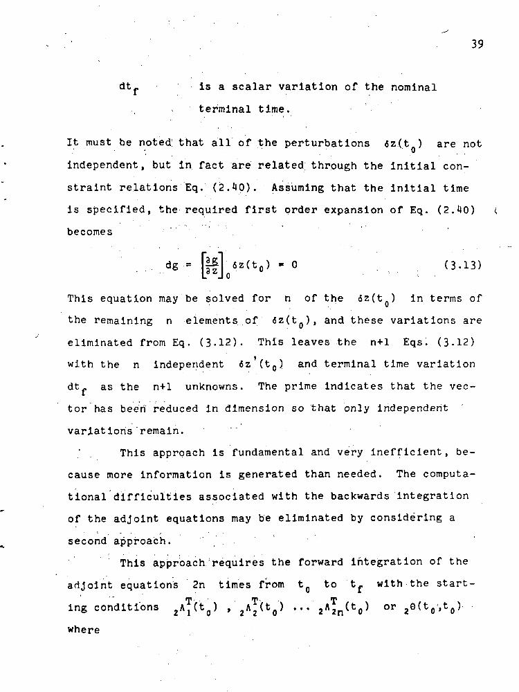
39
dtf is a scalar variation of the nominal
terminal time.
It must be noted; that all of the perturbations 6z(t ) are not
independent, but in fact are related; through the initial con-
straint relations Eq. (2. 0). Assuming that the initial time
is specified, the required first order expansion of Eq. (2.^0)
becomes
dg-»- fffl «z(t0) =0 (3,13)
This equation may be solved for n of the 6z(tfl) in terms of
the remaining n elements of fiz(t ), and these variations are
eliminated from Eq. (3.12). This leaves the n+1 Eqs. (3.12)
with the n independent 6z (tQ) and terminal time variation
dtf as the n+1 unknowns. The prime indicates that the vec-
tor has been reduced in dimension so that only independent
variations remain.
' . This approach is fundamental and very inefficient, be-
cause more information is generated than needed. The computa-
tional difficulties associated with the backwards integration
of the adjoint equations may be eliminated by considering a
second approach.
This approach/requires the forward integration of the
adjoint equations 2n times from tfl to tf with the start-
ing conditions 2A^'(tfl) » VJ^Q) •" 2A2n(to) °r 2e(t0',t0). •
where
1 0 0
0 1 0
0
0
0 0 0
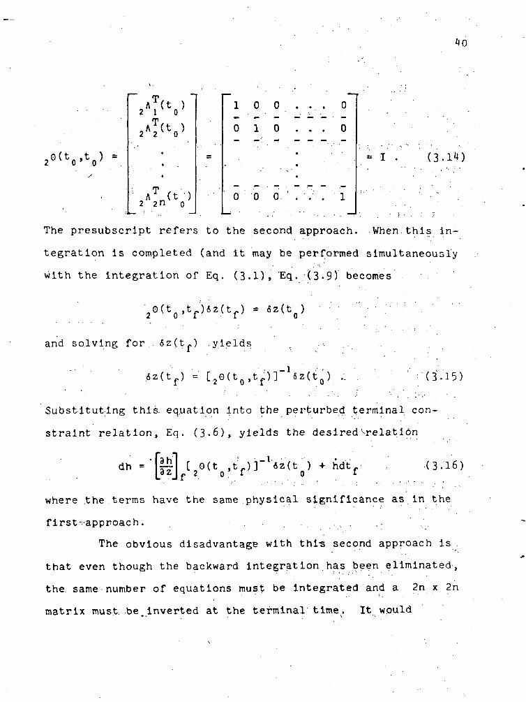
= I (3.1*0
The presubscript refers to the second approach. When this in-
tegration Is completed (and It may be performed simultaneously
with the integration of Eq. (3.1)> Eq. (3.9) becomes
2G(to,tf)6z(tf) = 5z(to)
and solving for . 6z(tf) .yields
_l«z(tf) = [20(t0,tf)] 6z(tQ)
1 ^ (3.15)
Substituting this, equation into the perturbed terminal con-
straint relation, Eq. (3.6), yields the desired^relation
dh ~1
f 2,t.)]~6z(t ) + hdt.
"(3.16)
where .the terms have the same physical significance as in the
first--approach. . . . ... ., .
The obvious disadvantage with thi-s second approach is .
that even though the backward integration/has been eliminated,
the. same number of equations must be integrated and a 2n x 2n
matrix must be inverted at the terminal time. It would
certainly be desirable if an approach could be formulated such
that the above matrix inversion is unnecessary and a more effi-
cient integration is made,
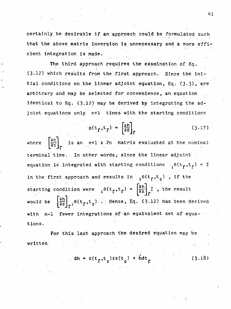
The third approach requires the examination of Eq,
(3.12) which results from the first approach. Since the ini-
tial conditions on the linear adjoint equation, Eq. (3-3), are
arbitrary and may be selected for convenience, an equation
identical to Eq. (3.12) may be derived by integrating the ad-
Joint equations only n+1 times with the starting conditions
•e(tf,tf) = |f|]f (3.17)
where | ~1 ^s an n+l x 2n matrix evaluated at the nominal
terminal time. In other words, since the linear adjoint
equation is integrated with starting conditions 0(tf,tf) = I
in the first approach and results in jO^f^g) > if< tne
starting condition were (t t ,) = U^- I , the result
would be 1^- ,e(t-,tn) . Hence, Eq. (3.12) has been derivedI o Z I -II 0
with n-1 fewer integrations of ;an equivalent set of equa-
tions.
For this last approach the desired equation may be
written ' ' '
dh 0(tr,t )6z(t ) + hdt (3.18)1 0 o r

where the terms have the same physical significance as the
previous two approaches, but O(tf,t0) is an n+1 x 2n matrix
resulting from the simultaneous backward integration of the
adjoint equations. Again the dependent initial state and/or
Euler variable variations must be eliminated, and this leaves
n initial variable variations and one terminal time variation
to be determined from the n+1 equations, Eq. (3.18).
The explanation for the third approach gives the Jus-
tification for the scheme used by Jazwlnski (12) where an ex-s~. •
tension is made of Jurovics and Mclntyre's (7) presentation.
One additional time conserving feature, which may be used, is
the scaling of the Lagrange multipliers. This advantage re-
sults because the Euler-Lagrange equations are.,linear, and, • .
homogeneous. The implementation .of this idea is discussed in..
Section 7.3 and essentially involves the trading of one termi-
nal condition for an initial condition. The decrease In the
dimension of the terminal constraint vector by one, also de-
creases the number of adjoint integrations by one, -and hence •
results in less computation- time. . -
One additional remark is in order for eases where the.
specified terminal constraints are rather..: complex and the
Lagrange multiplier v is introduced. For this case, the . ;
terminal constraint vector becomes
-• • • ' ' ' • . ' . ' ' • J • '
h = h(zf,tf,v) = 0 (3.19)

where h is an n+l+q vector, and the perturbed terminal con-
straint relation, Eq. (3.1*), becomes
dh = f
62 (V ;* hdtf + fdv ( 3 . 2 0 )
where — is an n+1 x q matrix evaluated at the nominalI— 1
terminal time and d\> is a q vector of total Lagrange multi-
plier variations. It should be recalled that when the v
vector is used, there exists n+l+q terminal constraint rela-
tions and this increases the dimension of the dh vector by
q . This is Just the number of additional equations needed to
solve for the additional unknown variations dv . These varia-
tions are applied to the assumed values of v .
A similar technique is used by Breakwell, Speyer, and
Bryson (9). It is shown in this reference that after the
forward integration of Eq. (3.1) has been made, q of the n
equations represented by Eq. (2.33) may be used to determine
the q values of v . Then these q values of \> are used
to evaluate the terminal dissatisfaction represented by the
remaining n-q equations of Eq. (2.33). This procedure simply
reduces the dimension of h to n+1 , arid hence only n+1
backward integrations of Eq. (3-3) are needed.
The computational procedure may be followed by re-
ferring to an illustration of the Method of Adjoint Functions
(MAP) :

•p.
Desired Terminal. Conditions"""
(1) Integrate the 2n nonlinear'differential equa-
tions of motion and the Euler-Lagrange equations, Eq.
(3.1), forward from tQ to t ' with starting condi-
tions satisfying Eq. (2.40) and n assumed values
for the unknown parameters.
(2)_ Evaluate at the nominal terminal time, tf , the
quantities h , h * and the starting .conditions for
the backwards integration of the adjoint equations,.
(3) Integrate the 2n adjoint equations, Eq. (3.3),'
backwards n+1 times from tf to tQ with 'starting
conditions, f-^ and use the value of the variables

stored during the forward integration to form the
coefficients of the adjoint variables.
. (4) Solve the n+1 linear algebraic equations, Eqs.
(3.18), fpr a linear approximation of the corrections
that must be applied to the assumed initial values
the terminal time. • ,
(5) Apply these corrections and repeat the process
until the corrections become smaller than some pre-
selected value.
3.2 _ Methods of Perturbation Functions
Of the several methods available for determining the
terminal variations in the state and Euler variables as a func
tion of the initial variations, i.e. 6z(tf) = [n]6z(tQ) , the
most natural one involves the direct use of the perturbation
equations, Eq. (3.2)
6z = A6z . , (3.21)
As a first approach, integrate these perturbation equations
forward from t to t-, 2n times with the starting condi-o f
tions
or

where ,to o
ll0|°l' 1
01
0.-1. 0
.
0
• • ' - . "
* * *
000
1
(3.22)
= I.
The presubscript refers to the first approach. This integra-
tion may be made simultaneously with the forward integration of
the differential equations, Eq. (3.1), and hence less computer
storage is required. When this integration is completed, the
resulting equations evaluated at the terminal time may be
represented by '.'.•'• . ; ••;...
:5z(tf) = 1*(t0,tf)6z(t(j) ,. - (3.23)
where *(t'0,tf) is a 2n x 2n matrix of partial derivatives
evaluated on the nominal trajectory. This equation may be
substituted into the perturbed terminal constraint relation,
Eq. (3.6), and the desired result becomes
dh = fiHl[ft]f i(3.2*1)
where the symbols have been explained previously. 'These n+1.
equations contain 2n initial state and Euler variable varia-
tions and one terminal time variation. However, the dependent
variations may be eliminated as explained for the adjoint
methods and only the n+1 independent variations must be
determined.
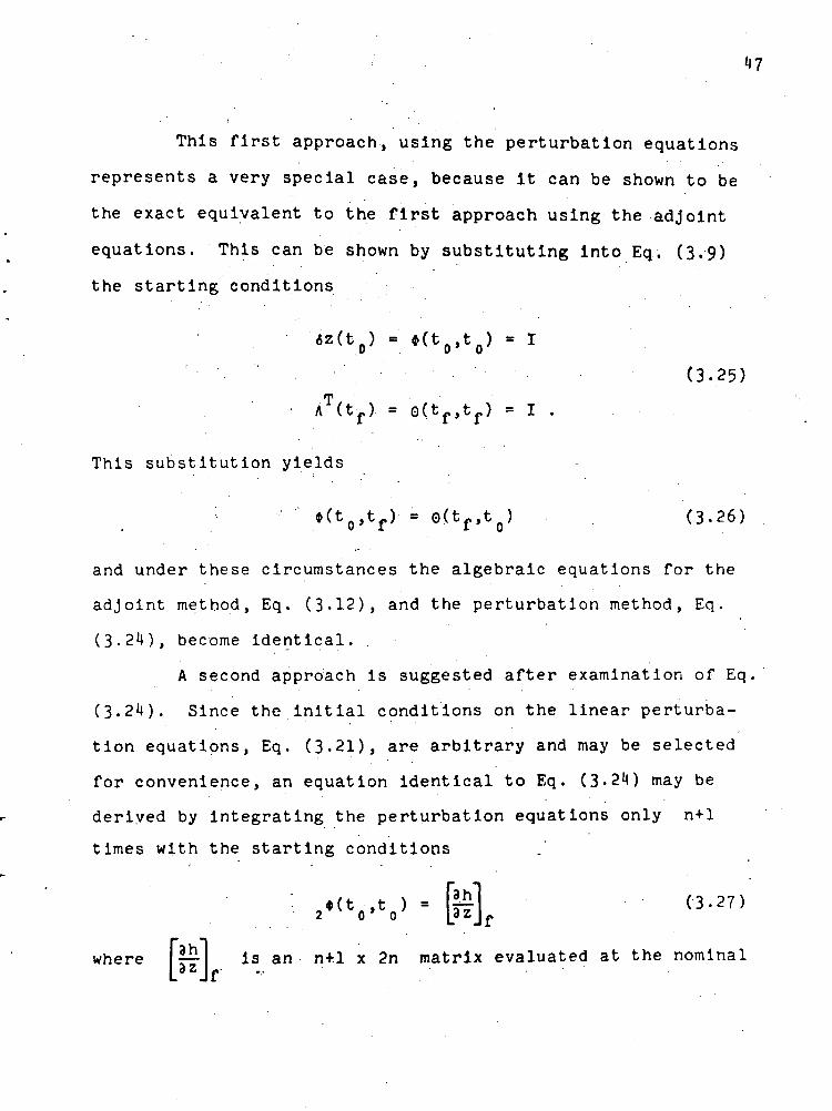
This first approach, using the perturbation equations
represents a very special case, because it can be shown to be
the exact equivalent to the first approach using the adjoint
equations. This can be shown by substituting into Eq. (3.9)
the starting conditions
6z(t0) = »(t0,t0)
AT(tr) = 0(tr,tr) = I .
(3.25)
This substitution yields
*(tQ,tf) = 0(tf,to) (3-26)
and under these circumstances the algebraic equations for the
adjoint method, Eq. (3.12), and the perturbation method, Eq.
(3.24), become identical.
A second approach is suggested after examination of Eq
(3.24). Since the initial conditions on the linear perturba-
tion equations, Eq. (3.21), are arbitrary and may be selected
for convenience, an equation identical to Eq. (3-24) may be
derived by integrating the perturbation equations only n+1
times with the starting conditions
NMrwhere \~\ is an n+1 x 2n matrix evaluated at the nominal

terminal time. The resulting linear algebraic equation to be
solved becomes . .
dh = -*(t ,tr)6z(t ).+• hdt ' ••-..-' (3.28)2 0 1 0 I
where <t>(t0,t_)' is generated by only n+1 integrations of
the perturbation equations. . . .
This approach loses some appeal, however,, when imple-
mentation 'begins because the starting condition, Eq. (3.27),
cannot be evaluated until a nominal trajectory is Integrated.
Since the perturbation equations cannot be integrated simul-
taneously with the differential equations, the nominal path
must be stored and no particular advantage over the adjoint
method is realized.
A third approach, which proves to be the most effi-
cient, may be formulated by observing the manner in which the
0(tf,t ) and <t>(t ,tf) matrices are generated and used.
For each of the n independent initial variations required a
corresponding column of the jOCt-.tg) or ^(t^t-) matrix
is needed. Since the 10(t_,tQ) matrix is generated by rows,
to determine any one column requires all 2n - integrations of
the adjoint equations. This, however, is not true for the per-
turbation methods, because the I*^t0»
tf^ matrix is generated
by columns. The elements of any n columns can be determined,
by simply integrating the perturbation equation n times, the
starting vector having the element that corresponds to the

desired initial unknown variation set equal to unity arid all
others zero. With this modification, the linear algebraic
equation becomes
dh = f-l'tCt-Vt-^z'Ct-) + hdtr (3.29)| O &\ « U 1 U X ;
where »(t0,tf) is a 2n x n matrix generated by, integrating
the perturbation equation only n times and 6z'(t ) becomes
an n vector representing the desired independent initial
variations.
The essential feature of the perturbation method is
that only n integrations are needed, and hence one less inte-
gration of a set of equations equivalent to the adjoint equa-
tions. The third approach to the adjoint method and the above
perturbation method require.the.solution of exactly the same
linear system, but the required elements of the »(tQ,tf)
matrix are simply derived in a more efficient manner. The
additional advantage of using the perturbation method is that
the nominal trajectory does not require computer storage.
The computational procedure may be followed by re-
ferring to an illustration of the Method of Perturbation
Functions (MPF):

Desired .Terminal
Conditions
(1) Integrate the 2n nonlinear differential, equa-
tions of motion and the. Euler-Lagrange equations, Eqt
(3.1)9 forward from t0 to tf with starting condi-
tions consisting of the n known initial conditions
satisfying Eq. (2. 0') and n assumed values for the
unknown parameters. • : ' •
(2) Simultaneously with the above integration, inte-
grate the 2n perturbation equations, Eq. (3-21),
with starting conditions described above and coeffi-
cients formed from the variables that describe the
nominal trajectory.

51
(3) Solve the n+1 linear algebraic equations, Eq.
(3.29), for a linear approximation of the corrections
that must be applied to the assumed initial values and
the terminal time.
(4) Apply these corrections and repeat the process
until the corrections become smaller than some pre-
selected value.
3.3 Iteration Philosophy for the Perturbation Methods
The iteration schemes for the Perturbation Methods simply
consist of a procedure for .iteratively determining the initial
values of the Lagrange multipliers so as to decrease the terminal
constraint dissatisfaction on the following iteration.. The con-
trol i? eliminated from the differential equations, Eqs. (2.23)
and (2.2^4), by using the optimality conditions, Eq. (2.25), and
the nonlinear differential equations are integrated during each
iteration. Since the optimality condition is always satisfied,
every iteration produces an optimal trajectory, but to an un-
desired terminal condition. The only remaining complication is
to satisfy the. desired terminal constraints, Eq. (2.U2).
Normally, the requested-change in-the terminal dissatis-
faction is equated to the negative of the terminal dissatisfac-
tion resulting from the previous iteration. This requested
correction is then used in the linear algebraic equations, Eqs.
(3.18) or (3.29), to make a multiple linear interpolation for

52'
the variations of the. initially assumed values o.f the state
and/or Euler variables. When these corrections are applied and
a new nominal trajectory integrated, the terminal constraint
dissatisfaction is usually reduced.
The difficulty with this type of indirect optimization
procedure is that when the terminal dissatisfaction is large,
the linear approximations are not very representative of the
nonlinear system, and the possibility for divergence is in-
creased. The linearization is made about the current nominal
trajectory, and whether or not this trajectory is close to
satisfying the terminal constraints on any given iteration is
immaterial. The essential factor is that the trajectory re-
sulting in the next iteration be sufficiently near the previous
one so that the linearization assumptions are not stretched
beyond the limits of validity.
One natural approach, the motive for which resulted
from a suggestion made by Breakwell, Speyer, and Bryson (9), is
to request the correction of only a percentage of the terminal
dissatisfaction resulting from the previous iteration. For
instance, the algebraic equation that contains the corrections
for the Method of Perturbation Functions is
dh = j|£J »(t0,tfi)6z(t6) + hdtf (3-30)
and for a percentage correction let
dh = -ch (3-3D

53
where c is the desired percentage to be corrected. The
iteration factor c may. have values in the range 0 < c < 1.
A correction for the Method of Adjoint Functions Is applied In
the same manner.
It is also reasonable to expect that as the optimal tra-
jectory is approached, successive trajectories will be suffi-
ciently near one another. Hence, the linear representation
becomes accurate enough to request the complete correction of
the terminal dissatisfaction. Also,.as successive trajectory
iterations begin to converge, successive adjoint and perturba-
tion solutions begin to converge, and hence integration of
these equations for every iteration may be unnecessary.
A summary and extension of the conjectures stated
above, which result in some of the desired characteristics of
an iteration scheme, are that:
(1) An iteration factor may be specified initially
and changed during subsequent iterations by specifying
an iteration rate factor. As the iterations proceed,
the iteration rate factor is used to control the per-
centage of the terminal dissatisfaction corrected on
any given, iteration.
(2) There may exist an initial value of the iteration
factor that minimizes the convergence time or maximizes
the chance for convergence.

(3) It may be unnecessary to update the *(t,tf)
and 0(tf,t ) matrices on every iteration.
CO A correction of more than 100 percent may be
reasonable and desirable.
These conjectures are investigated by using the following dif-
ferent iteration schemes:
. Iteration Scheme 1 - This scheme for both the Methods
of Adjoint and Perturbation Functions requires the arbitrary
selection of an initial value of the iteration factor and the
iteration rate factor. An iteration is made and the corre-
sponding iteration factor is applied to obtain corrections for
the next iteration. If the norm of the terminal dissatisfac-
tion decreases on the next iteration, the iteration factor is
increased by the value of the iteration rate factor. This
process is repeated, never allowing the iteration factor to be
zero or greater than unity, until the corrections for each
assumed value is less than some preselected value.
A detailed procedure of Iteration Scheme 1 follows:
(1) Starting values of the iteration factor and the
iteration rate factor are selected.
(2) Integrate th'e nonlinear differential equations of
motion forward, noting the norm of the terminal dis-
satisfaction. If the Method of Adjoint Functions is

55
being used, integrate the adjoint equations backwards.
If .the Method of Perturbation Functions is being used,
the perturbation equations may be integrated forward
simultaneously with the differential equations of
motion.
(3) Solve the algebraic equations, using the specified
value of the iteration factor, to determine the correc-
tions required for the initially assumed values.
CO If all corrections are less than some preselected
value, terminate the iteration. If any one correction
is greater than the preselected value continue the
process as follows.
(5) Apply the corrections to the assumed initial con-
ditions, integrate the differential equations again,
and determine the terminal dissatisfaction. If the
norm of the terminal dissatisfaction is less than the
norm that results on the previous iteration, increase
the iteration factor by the value of the iteration
rate factor and continue to iterate. Never allow the
iteration factor to be greater than unity.
(6) If the norm is greater than the previous norm,
decrease the iteration factor by the value of the
iteration rate factor and continue to iterate. Never

56
allow the iteration factor to be less than the value
of the iteration rate factor.
Iteration Scheme 2 - During the initial efforts to
solve a problem with either the Method of Adjoint Functions or
the Method of Perturbation Functions, a low initial value for
the iteration factor is usually assumed. This requests a small
change from a solution which is probably far from optimal, and
thus reduces the possibility for divergence. However, this
could be an unreasonably low estimate and if the iteration fac-
tor is systematically increased, as in Iteration Scheme 1, a
great number of iterations would be required before a full
correction would be requested. This scheme reduces the con-
vergence time by avoiding the integration of the perturbation
or adjoint equations on certain iterations. The criterion used
to establish when a perturbation or adjoint equation integra-
tion is made is that either a divergence of the terminal con-
straint norm occurs or the integration is forced after a
specified number of corrections have been made. The iteration
factor is still increased each time a norm convergence occurs
and the trajectory that produces this convergence is called a
nominal. When the terminal norm diverges the iteration factor
is decreased and the last convergent trajectory is used as a
nominal. ' . • . .

57
A detailed procedure of Iteration Scheme 2 follows:
(1) Starting values of the Iteration factor and the
iteration rate factor are selected.
(2) Integrate the nonlinear differential equations of
motion forward,.noting the norm of the terminal dis-
satisfaction. If the Method of Adjoint Functions is
being; used, integrate the adjoint equations backwards.
If the Method of Perturbation Functions is being used,
the perturbation equations may be' integrated forward
simultaneously with the differential equations-of
mot ion:.
(3) Solve the algebraic equations, using the specified
value of the iteration factor, to determine the correc-
tions required for the initially assumed values.
CO If all corrections are less than some preselected,
value, terminate the iteration. If any one correction
is greater than the preselected value continue the
process as follows.
(5) Apply the corrections to the assumed initial con-
ditions, integrate the differential equations again,
and determine the terminal dissatisfaction. If the
norm of the terminal dissatisfaction is less than the
norm that results on the previous iteration, Increase

58 '
the iteration factor by the value of the iteration rate
factor. If the Method of Adjoint Functions is being
used, avoid the adjoint integration on the present
iteration. If the Method of Perturbation Functions is
being used, avoid the perturbation integration on the
next iteration.
(6) If the norm is greater than the previous norm, or
if a specified number of iterations have been made, de-
crease the iteration factor by the value of the itera-
tion, rate factor. If the Method of Adjoint Functions
is being used, the adjoint equations are integrated
backwards where the coefficients are obtained from the
last convergent forward trajectory. If the Method of
Perturbation Functions is being used, the perturbation
equations are integrated on the next iteration.
CHAPTER 4 - • . .
QUASILINEARIZATION .METHODS
The.previously discussed Methods of Adjoint and Pertur-
bation Functions' involve the integration of a set of nonlinear
differential equations. The coefficients for the linear
adjoint or perturbation differential equations are formed with
the variables generated by the nonlinear equations. A.somewhat
different approach can be formulated by linearizing the differ-
ential equations, and then using the adjoint and perturbation
functions in the same general manner as before. The coeffi-
cients used to generate a new nominal trajectory are formed
from the solution that corresponds to the previous nominal tra-
jectory. This , .essentially , is the quasilinearization concept.
The theoretical development of the Quasilinearization
Methods may be shown to follow common lines, and in this sense
the formulations are parallel. The approaches involve the
solution of a set of linear differential equations, the solu-
tion of which converges, under appropriate conditions, to the
solution of the desired nonlinear problem. Since the equations
are linear, the terminal constraints can be satisfied on every
iteration, if. desired. However, the .classical optimality con-
dition is not satisfied until convergence has occurred, and
even though the end points of the trajectory are satisfied,
some care must be taken to insure that the trajectory shape
59
6o
between these end points is correct. One other characteristic
of the quasilinearization techniques is that an initially
assumed solution is required. If a reasonable estimate of the
solution cannot be made, a starting solution, derived from the
integration of the nonlinear differential equations, may be
good enough" to result in convergence. This requires that only
the initial values of the unknown variables be assumed, rather
than the complete"solution.
*4.1 Methods of Generalized Newton-Raphson
The complete solution of the two-point boundary value
problem by using' the Method of Generalized Newton-Raphson may .
be obtained in a manner similar to the Method of Perturbation
Functions discussed in Section 3-2. The exception to this
similarity is that the differential equations, Eq. (3-l)> aret
linearized about the previous nominal. .
The problem is formulated in terms of an ordinary first -
order, nonlinear, vector, differential equation
z = F(z,t) (4.1)
where z is a 2n vector composed of n state variables and
n Euler-Lagrange variables and: t Is the independent variable
time. This nonlinear equation may be expanded about the pre-
vious nominal trajectory, say the n trajectory, and by
ignoring the nonlinear terms yields .

61
= zn +.A(zn,t)(zn+1 - zn) (4.2)
• ' . TSP"!where A(zn,t) is the partial derivative matrix hp- •
This matrix is evaluated on the previous nominal trajectory
and is similar to the A(z,t) matrix discussed in the develop-
ment of the Perturbation Methods. This equation, Eq. (4.2),
can be expressed as
( z = Az + B (4.3)
where A is described above and B = z - Az . Note that A
and B are known from the previous nominal trajectory.
The first approach to the Method of Generalized
Newton-Raphson is similar to the method outlined by McGill and
Kenneth (13), and this provides a starting point for further
development. Suppose that p of the initial values of z are
specified, i.e. z.(t ) = z. , i = 1, p . This implies that
2n-p initial values of z must be assumed along with an
assumed value of initial time tQ . The homogeneous part of
Eq. (4.3) may be expressed as
y = Ay . . "' (4.4)
and hence it is.similar to the perturbation equations, Eq.
(3.21). Eq. (4.4) may be integrated forward from tQ to tf
2n-p times with each successive starting vector consisting of

all zero elements except for the element that corresponds to
one of the unknown- initial 'conditions. This element is set
equal to unity. This procedure leads to a 2n x 2n-p matrix
of solutions Y'(t ,t) . The forward integration amounts to
making a unit perturbation in each one of the unknown initial
conditions. -
The nonhomogeneous solution to Eq. (4.3) may be ob-
tained as a solution to
/
w = Aw + B (4.5)
which generates a particular solution when integrated from t.U
to tf with the p known initial conditions and n-p assumed. • ' ' -. " ^ • • t .. .
initial conditions. Now, the general solution of the linear
system of Eqs. (4.3) becomes
z(t) = Y(to,t)C + w(t) . - (4.6)
where z ,is a 2n vector of .state and Euler variables, Y is
a 2n x 2n-p, matrix of homogeneous solutions, C is a 2n-p
vector of. constants arid w is a 2n vector of nonhomogeneous
solutions. —
Since 2n-H-p conditions on the terminal value of z
must be specified for a variable final time problem, any 2n-p
of these conditions may be selected and the appropriate 2n-p
members of Eq. (4.6) may be evaluated at the assumed terminal
time. Then these equations are solved for' the1 2n-p constant
corrections C . These corrections are used to update the

63
assumed initial conditions for the next iteration. For the
purpose of saving computer storage the nominal trajectory is .
not formed by the linear combination of Eq. O.6), but by in-
tegrating Eq. (U.3) with the updated initial conditions. This
requires only the storage of the final values of the homogene-
ous and nonhomogeneous solutions.
This procedure is continued until a metric (that repre-
sents the maximum distance, over the complete independent
variable range, between successive nominal trajectories) be-
comes less than some preselected value. This metric is given
by
P =N£1=1
maxt '
Jn+i - z"n (1:7)
Since this metric represents the maximum distance between suc-
cessive nominal trajectories, its value decreases as the opti-
mal trajectory shape is converged upon. When this metric has
been reduced to an acceptable value, convergence has occurred
for the specified value of terminal time. The .one remaining
unused terminal condition is used in a conventional scalar ap-
plication of the Newton-Raphson iteration technique to produce
a more accurate determination of terminal time. This finite
difference equation is , .
k+i
Z^-J
(1.8)

where the subscript k refers to the kth time iteration and
zf Is the desired terminal value of the variable selected.
This new terminal time is used and trajectory iterations are
made until the metric p is reduced once again. When the
time iterations result in time changes smaller than some pre-
selected value, the desired solution has been determined and
the procedure is terminated.
One of the principal differences of the Method of
Generalized Newton-Raphson as opposed to the Perturbation
Methods is that an initial solution of the state and Euler
variables is required. Also the method by which the terminal
time is determined is very time consuming, especially when a
large error is made in the assumed terminal time. A major ob-
jection is that the initial and terminal conditions must simply
be values of the variables involved, rather than general func-
tions of these .variables. The 'above stated difference- can be
avoided, in some cases,-by simply using the solution generated
by integrating the nonlinear equations, Eq. (4:1), and this
approach requires only starting values of the variables, p
of which are known/ The above stated objection has been par-
tially removed by L6ng-(l6). •
The method proposed by Long, designated here by the
Modified Method of Generalized Newton-Raphson, involves a
change of the independent variable
. t = as . (4.9)

6
where a is a constant and s is a new independent variable
having values 0 t s 1 . The differential equations, Eg.
(4.1), now become
f\7z' = |f = aFCz,as) , • (4.10)
The constant a is considered a .new state variable and an
additional differential equation
a ' = 0 . . . . . • • (4.11)
may be added, but this is clearly not necessary since the solu-
tion to this equation is trivial. The value of a is initially
assumed and then corrected on each iteration Just like any other
initially unknown state variable. The value a represents the
terminal time as can be seen by evaluating Eq. (4.9) at the
terminal .value of the independent variable.
The determination of the terminal time now becomes an
integral part of the iterative scheme, and its separate con-
sideration, as required by the first approach, is not required.
However, this does not save as much time as one might think,
since a term that corresponds to the new state variable a
must be added to each differential equation. Also another in-
tegration of the 2n homogeneous equations must be made since
the value of a must be iteratively determined. The other
objections discussed for the first approach are not

66
eliminated. The effectiveness of Long's proposal is evaluated
and discussed further in a later chapter.
4.2 _ Modified Quaslllnearlzation Method
The method proposed in the present study, called the
Modified Quasilinearization Method, uses the quasilineariza-
tion concept but removes the restrictions on the Methods of
Generalized Newton-Raphson discussed in Section 4.1. The
manner in which the terminal time is determined proves superior
to the modification proposed by Long.
The Eq. (4.6), derived for the Method of Generalized
Newton-Raphson, can be rewritten and evaluated at the terminal
time
Y(t0,tf)C = z(tf) - w(tf) . (4.12)
The right hand side of this equation Is the difference between
the desired terminal value of z and the linear calculation
of the terminal value of w . This difference is interpreted
as the variation of z(tf) , and is expressed as 6z(tf) .
Now, if both sides of Eq . (4.12) are premultiplled by h^r >
the resulting expression becomes
where — is a 2n+l-p x 2n matrix describing the partialL3ZJf-
change of a general set of terminal boundary conditions,

67
h(zf,tf) , to a.change in,the terminal values of zf Itself.
The right hand -.side of Eq. (4.13) is. the variation of this
general set of terminal boundary conditions 6h(tf) . A first
order expansion of the terminal boundary conditions may be•
made, dh = 6h + hdtf , and substituted into Eq. (4.13) to
yield
= [ft] Y(t0»tf)C + hdtfdh =
where dh is a 2n+l-p vector of terminal constraint dis-r
satisfaction, ^- is an 2n+l-p x 2n matrix of partial de-
rivatives, Y(t0,tf) is an 2n x 2n-p matrix of the terminal
values of the homogeneous solutions, C is a 2n-p vector of• •
corrections to be determined, h is a 2n+l-p vector of
time rates of change of the terminal constraints and dtf is
the time correction to be determined.
The Eq. (4.14) just derived is analogous to Eq . (3-29)
developed for the Method of Perturbation Functions. The major
exception is that in the present case the nonlinear differen-
tial equations of motion and the Euler-Lagrange equations are
linearized. If the optimization problem is reduced to a two-
point boundary value problem as discussed in Section 2.2, . ,p
becomes equal to n and the implementation of the two .methods
is similar. - - . .

68
The computational procedure may be followed by re-
ferrinc 'to an illustration of the Modified Quasilinearization
Method (MQM)": • . :
(1) Integrate the 2n linear nonhomogeneous different
tial equations, Eq. (4.3), forward from . t-0 to t«
with .starting conditions consisting of. the n- known
initial conditions and n assumed values for the un-
known parameters. The A and B matrices are
evaluated from the previous.nominal (on the first
iteration the assumed nominal is used).

69
(2) Integrate the 2n linear homogeneous differen-
tial equations, Eq. (^.4), forward, simultaneously
with the Eq. ('1.5), from t0 to tf with n start-
ing conditions consisting of a unit perturbation of
• the variables'that corresponds to the unknown initial
conditions.
(3) Solve the n+1 linear algebraic equations, Eq.
(4.1*1), for a linear determination of the corrections
that must be applied to the assumed initial values and
terminal time.
(*0 Integrate the 2n 'linear nonhomogeneous differ-
ential equations, Eq. (^.3), forward from t to
t~ + 6tf with the initial conditions updated by the
recently calculated corrections. This integration*
yields a new nominal.
(5) The process is continued until the metric p
and the corrections become less than some preselected
values.
It should be noted that this approach could have used( '
the adjoint functions rather than the perturbation functions.
In this case, its implementation will require the use of a
set of equations adjoint to 'the homogeneous equations, Eq.
(Jj.'O, and its development runs parallel to the method

70
discussed in Section 3.1. The algebraic equation to be solved
becomes . . . . , - • •
dh = o'(tf,t0)«z(t0) + hdtf '' ' (H
iwhere 0 is an n+1 x 2n matrix resulting from the simul-
taneous backward integration of the adjoint equations.
1. 3 Iteration Philosophy for the Quasillnearlzatlon Methods
The iteration scheme for the Quasllinearization Methods
simply consist of a procedure to iteratively determine the
Initial values of the Lagrange multipliers so as to decrease
the metric p . The control is eliminated from the differen-
tial equations, Eq. (1,1), by using the optimality conditions,
Eq. (2.25), and the linearized differential equations are in-
tegrated during each Iteration. Even though the optimality
conditions are used, the trajectory iterations do not repre-
sent optimal solutions because the trajectories are generated
from a linearized version of the nonlinear differential equa-
tions. The only'remaining requirement is to reduce the metric
p to an acceptable value, which means that an optimal solution
has been converged upon.
With the Method .of Generalized Newton-Raphson, the
terminal values of the desired variables are introduced and
essentially forced to, satisfaction on each .iteration. The
metric p is reduced to an acceptable value by iterating on
an assumed value of terminal time. Then one of the desired

71
terminal values Is used In a scalar application of the Newton-
Raphson method to determine a new terminal time.
Iteration Scheme 1 - This scheme is used with the
Method of Generalized Newton-Raphson, and is one which allows
a time iteration to be made while the metric P is being de-
creased. This scheme effectively reduces the metric p in
conjunction with convergence on the desired terminal time.
A detailed procedure of Iteration Scheme 1 follows:
(1) Assume a solution for the 2n trajectory
variables and a terminal time.
(2) Make one trajectory iteration by integrating
forward the homogeneous and nonhomogeneous equations,
Eqs. (4.4) and (4.5), respectively. Determine the
corrections and integrate the nonhomogeneous equation
once again with the new initial conditions. This last
integration is considered a new nominal and the metric
p is determined for this nominal and the assumed
trajectory.
(3) Make one more trajectory iteration and obtain a
new metric, p .
CO Using one of the desired terminal values make a* * ' * - -
Newton-Raphson iteration to obtain a new value of
terminal time.'

72
(5) Make two more trajectory iterations and record
the value of the metric p, .
(6) If the metric p3 is less than the metric p ,
make another time iteration and.continue the process.
(7) If the metric. p3 is-greater than the metric . •• .
p , continue the. trajectory .-iterations until the
metric becomes less than p2 . Then make a time
iteration and continue the process.
(8) Terminate the procedure when the time corrections
and the current metric become less than some pre-
selected values.
Iteration Scheme 2 - This scheme is used on the Modi-
fied Quasilinearization Method and is similar to Iteration
Scheme 1 presented for the Perturbation Methods. When the
MGNR is used, the terminal values of the desired variables are
introduced in such a manner that a full correction is requested
on every iteration. It is expected that if a full correction
is requested in cases where the linear representation is poor,
the sequence of linear solutions will diverge. The less
severe request of only a percentage correction is applied with
the Modified Quasilinearization Method and the linear algebraic
equation that contains the n+1 corrections is

73
dh = [ft] Y(t0,tf)C + hdtf .
The terminal dissatisfaction change for a percentage correc-
tion is
. fdh = -ch
where c is the desired percentage to be .corrected, and the
iteration factor c may have values in the range 0 < c < 1 .
A detailed procedure of Iteration Scheme 2 follows:
(1) Starting values of the iteration factor and the
iteration rate factor are selected. Assume a solution
for the 2n trajectory variables, and a terminal time.
(2) Make one trajectory iteration by integrating
forward the homogeneous and nonhomogeneous equations,
determining the corrections and Integrating the non-
homogeneous equation once again with the new initial
conditions and new terminal time. This last integra-
tion is considered a new nominal and the metric p
is determined for this nominal and the assumed tra-
jectory.
(3) If all the corrections and the metric p are
less than some preselected values, terminate itera-
tions. If any one correction or the metric p is

greater than the preselected value continue the
process.
CO Apply the corrections and make another trajectory
iteration, obtaining a new metric p .
(5) If the new metric is less than the old metric,
increase the iteration factor by the value of the
iteration rate factor and continue to iterate. Never
allow the iteration factor to be less than the value<-\
of the iteration rate factor or greater than unity.

7
CHAPTER 5
GRADIENT METHODS
The general theory of the gradient concept is now both
well known and widely used for the approximate solution to
trajectory optimization problems. These methods have a common
characteristic in that the influence function concept is used
to determine how the performance index and/or a combination of
the terminal constraint relations are changed as the control
variables are changed. Then a control step is taken in the
negative gradient direction, i.e. the direction of steepest
descent, so as to extremize the performance index while satis-
fying certain specified terminal constraint relations.
The implementation of the gradient techniques has been
widely varied and relatively arbitrary because although the
gradient direction is well defined, the proper sized step in
control space is not. The convergence properties of'the methods
are dependent on Judicious selection of this step size and the
manner in which it is changed, and several efforts have been
made to improve the rather slow terminal convergence of the
gradient methods. Unfortunately, because of this inherent
arbitrariness in the gradient method, a great amount of human
intervention is required to select a proper control step size
and still avoid violating the linearity constraints imposed

76
on the problem. In this sense the implementation of the
gradient techniques is an art.
The theoretical development of the gradient techniques
discussed here may be shown to follow common approaches. The
primary difference being the manner in which the terminal con-
straints are handled and.the method of selecting the control
step size. The Method of Steepest Descent uses the terminal
constraints in the so-called "hard" form, i.e. the. constraints
are to be satisfied identically. The Modified Method of
Steepest Descent uses the terminal constraints in the so-
called "soft" form, i.e. the .constraints may be only approxi-
mately satisfied. -
5 .1 Method of Steepest Descent
The theoretical development of the Method of Steepest' f •- • ' ' ',
Descent is well known as discussed in References 17 through
21, and is summarized here only to provide background for thev
iteration scheme modification. It is desired to determine the
control program u(t') , where u is a m vector, which will
yield an extreme value of some performance index
* = *(xf,tf) " . (5.U
subject to the differential equations of motion'
x .= f(x,u,t) , "(5.2)
77
where x 'is an n vector while satisfying the terminal con-
straint relations
* = v(xf,tf) =0 (5-3)
where Y is a q vector. One of the desired terminal con-
straint relations may be. used as a stopping condition,
n = n(xf,tf) = 0 (5.1)
The integration process continues until this . stopping condi-
tion is satisfied. If the differential equations, Eq. (5.2),
are linearized about some nominal path, the resulting equa-
tions become ,
6x = F6x + G6u (5.5)
where F and G are n x n and n x m matrices of partial
derivatives evaluated on the nominal trajectory, respectively.
The equations adjoint to Eq . (5.5) are
X = -FTX (5.6)
where x is an n vector of adjoint variables. This equation
may be combined with Eq. (5-5) by premultiplying Eq. (5.5) by
TX and post multiplying the transpose of Eq. (5.6) by <5x
and adding the equations to yield
= XTG6u . (5.7)

78
Integrating Eq. ( 5 - 7 ) from tQ to t ' f yields
( X T 6 x ) f = / xTG5udt + ( X T 6 x ) 0 . ( 5 . 8 )fco
The boundary conditions on the adjoint variables are arbitrary
and may be chosen for convenience. The object now is to de-
termine how initial state variations and integrated control
variations influence the terminal values of the performance
index, stopping condition and the terminal constraint rela-t • '. . ' • • ; '
tions. If, on separate trials, the terminal values of the
adjoint variables are set equal to
where X. is an n vector, X... is a nxq matrix and X09 ™ • "
is an n vector, the desired relations are seen to be
idt. (5.10)* '
i:: Ydtf
/
* m m •xi,G6udt + (\n6x) •»• ndtr (5-12)M n o i .

79
where
(5a3)
= \£* + Kr]f-
•[!£* If],
and
(5 .16)
•dy = [6* + *dt3f (5 .17)
dn = [5n + fldt]f . (5.18)
The approach presented by Bryson and Denham (18) allows
for the specification of a requested terminal dissatisfaction
improvement and an allowable step size to be taken in control
space. The control step size is defined by
dS = I |6uT W 6U dt (5-19)•'t o
where the step is a weighted quadratic function of the control
deviation. The weighting matrix W is included to improve
the., convergence characteristics by giving more weight to
regions of low sensitivity. However, it is often chosen to
be the unity matrix because of the lack of knowledge

80
concerning the region sensitivity. The criteria used for de-
termining the best elements of this matrix are not given and
are found through trial and error procedures.
The stopping condition, Eq. (5. ), is to be identically
satisfied so Eq. (5.12) is equated to zero. The terminal time
variation dt. is eliminated from Eqs. (5.10) and (5.11) to
yield
'0
.t.
(5.20)
(5.21)
where _n (5.22)
(5.2 )
The total variation in the performance index due to
initial state variations and integrated control variations
may be expressed as
dS ftfl T- / |6UTW
•'t.
(5
6udt

81
where the terminal constraint and the control step relationsm
are adjoined by the use of the v and y Lagrange multi-
pliers, respectively. The multiplier v is a q vector and
v is a scalar constant. Since it is desired to determine the
control variation which corresponds to the maximum change in
the performance index, the first variation of Eq. (5.21*) must
vanish
£•• G - -. y«uTW)62udt = 0 . (5.25)
This implies that the desired control variation is
6u = 1 W"1GT(x - X v) .
y $n T»(5.26)
When this equation is substituted back into Eqs. (5.19) ana
(5.21) the values of v and v are determined as
(5.2.7)
T - 1~
ds -
where
de
£'•(5.29)
(5.30)

/•tf:»* = / ; (5.3D
(5.32)
and Ivv is q x q matrix, I..,, is a q vector and I, .Y Y T y (f) (J>
is a scalar.
Now, combining Eqs. (5.26) through (5-32) yields the
desired control program
6u = *
+ w- 1Gx y ni;d6 ;. (5.33)
where the positive sign is used if 41 is to be maximized and
the negative sign used if $ is to be minimized. The pre-
vious control program is now modified as follows:
0
unew = uold * 6u '
The computational procedure for the Method of Steepest
Descent may be summarized by considering the following:
' \(1) Integrate the n differential equations of
motion, Eq. (5.2), forward in time using an assumed
control program and the desired initial conditions

83
for the state variables. This integration is con-
tinued until the stopping condition, Eq. (5.*0, is
satisfied. The value of the state variables aret
stored at each point in time.
(2) Integrate the n adjoint equations, Eq . (5.6),
backward q+2 times with the starting conditions,
Eq = (5.9). The coefficient matrix F is obtained
from the nominal generated on the forward integration
(3) Integrate the Eqs. (5-30), (5-31) and (5.32)
backwards simultaneously with the adjoint equations
using zero as initial conditions to yield the values
for Iy4, , Iy^ , and 1^ .
CO Select a desired improvement in the terminal
dissatisfaction dv for the next iteration.
(5) Select a reasonable value for the mean square
control deviation from the previous control program
by using
dS = W6u'(tf - t0) .
This will provide a value for the control step dS .
(6) Use the selected values of dv and dS to cal-
culate the numerator under the radical in Eq . (5-33)-
If this quantity is negative, determine the dY that

8')
makes the quantity vanish. It is is positive, use
the quantity as it is.
(7) Calculate the 6u as given in Eq . (5-33) and
alter the assumed control program.
08) This procedure is continued until the control
variations are less than some preselected value.
5.2 Modified Method of Steepest Descent
The theoretical development of the Modified Method of
Steepest Descent, which uses the penalty function technique
for handling the terminal constraints, is similar to the con-
ventional method discussed in Section 5.1. The primary dif-
ference is that the terminal constraint relation is included,
in the "soft" 'form, with the performance index to form a
penalty function
2P(xf,tf) = W0<t> (xf,tf) + W1v(xf,t (5.35)
where the W.'s are weighting constants. If these constants
are sufficiently large, minimizing the penalty function is
essentially the same as minimizing the performance index •$
and driving the terminal constraints f to zero.
To determine how this penalty function is related to
initial state variations and the integration control variations,

the" Eq. (5.8) is used. Selecting the terminal boundary condi-
tion for the adjoint equations, Eq. (5.6) to be
••> • KL. (5.36)
Xji(tf) - |j|J (5.37)
where Xp is an n vector and X is a scalar, yields
r:dP «'/ XpGfiudt -f ( X p 6 x ) Q + Pdtf (5 .38)
.tA rp m «
'Swhere
(5.40)Hi* ft
The stopping condition, Eq. (5-39), must be identically satis-
fied. Hence dt can be determined from Eq. (5.39) and used
to eliminate dt. from Eqs. (5.38). The result can be ex-
pressed as
/"'dP - / xJflG6udt + (^pn«x)0 (5-^2)

86
where
. , (5.13)
Now, it is desired to determine the control variation
which maximizes the change in the penalty function dP . To
insure the predominance of first order effects, a control step
size constraint is adjoined to the total variation of the pen-
alty function, to obtain
(5.1D
dP = dS rfi -- • / ?*"•^t.6udt
If the above Eq. (5-11) is to assume a^maxlrnum value, the
first variation must vanish, or
t
S(dP) = / '<*Jtn
- y6uT)62udt = 0
which implies that
6u = '(5.16)
where K is a constant equal to 1/p . This expression could
be written
6u = KHu (5.17)
where H is defined as the generalized Hamiltonian, xpnG • '

This equation implies that the control variation which
maximizes the penalty function change is proportional to the
magnitude of the control gradient and in either the positive
or negative gradient direction, depending on the sign of K .
The constant K may be Interpreted as the control step size
in the gradient direction. When the gradient H approaches
zero, the control variation also vanishes.
The penalty function change is evaluated by substi-
tuting Eq. (5.4?) into Eq. (5-42) to yield
rtfdP « K I HUH-J dt . (5.48)
fco
The computational procedure for the Modified Method
of Steepest Descent may be summarized by considering the
following:*
(1) Integrate the n differential equations of
motion, Eq. (5.2), using an assumed control program
and the desired initial conditions of state. This
Integration Is continued until the stopping condition,
Eq. (5.*»), is satisfied.
(2) Integrate the n adjoint equations, Eq. (5-6),
backward one time with the starting condition, Eq.
(5.«3), or

88
T1 I « A f l l i f lu A. i ft
forming the coefficient P from the nominal path , .
generated on the forward integration.
(3) Having obtained the solution *pn(t) the term
THU = Xpf}G may be formed.
T(4) The square of *pn
G ™ay be integrated from t0
to tf . Then, using Eq. (5.'l8), the step size K
may be determined by specifying a desired penalty
function change dP .-
(5) The control variation may be determined.from Eq
(5.^7) and applied to the assumed control program.
(6) The procedure continues until the penalty func-
tion reaches a minimum.
It must be noted that the specified penalty function change,
and hence the step size K is arbitrary, and the Judicious
selection of K becomes a key factor in Increasing the con-
vergence rate. An automatic procedure for its selection is
desired.

89
5.3 Iteration Philosophy for the Gradient Methods
The iteration schemes for the gradient methods simply
consist of a procedure to iteratively determine a control pro-
gram so as to extremize a performance index while simultaneous-
ly driving the terminal constraint dissatisfaction to zero.
The nonlinear differential equations of motion are integrated
during each iteration, and the adjoint equations are used to
determine how the variation of different terminal quantities
are influenced by Initial state variations and integrated con-
trol variations. The optimality condition, H =0, is not
used in the formulation, and hence is never identically satis-
fied.
A minimization of performance index requires a control
step to be taken in the negative gradient direction, con-
sistent with the specified terminal constraints, but the size/
of this step is not defined by considering the theoretical
development of the gradient technique itself. Hence, the most
severe disadvantage of these techniques is the arbitrariness.
Usually a satisfactory convergence rate can only be achieved
by experienced personnel.
A primary objective of the present study is to develop
an iterative scheme that removes some of the arbitrariness, and
increases the convergence rate. Since the weighting matrix
W , introduced in Eq. (5.19) is arbitrary, some rational basis
for its selection is needed. This problem is approached by

90
examining an integral form of the Weierstrass E-Function which
approximates the change in the performance index or the penalty
function. This change is approximated by
dP* 21 / E(x", x", x,t)dt (5.^9)f f «• •« •/ E(x , x , x
*tA'0
whore E is the Weierstrass E-Function as developed by Gelfand
and Fomin (27). The E-Function is defined as
E = F(x*,x,t) - F(x*,x*,t) - i£ (X*,x*,t)(x.-x*) (5-50)3x*
and for the system being considered
F(x,x,t) = H(x,u,t) - xTx , (5.51)
Twhere H = \ f . The asterisks refer to the optimal path, and
the absence of asterisks refer to any nearby path. From the-
calculus of variations a necessary condition for the existence '
of a minimum value of performance index is that E be non-
negative during the interval t ^ t t« •.
It is noted, by examining Eq. (5-2), that a -variation•
in control is accompanied by a variation in x , and that a
state variation will occur only after^a finite duration of
time. Hence, the expansion of Eq. (5.^9) is made by consider-
ing that the control deviation is not accompanied by a change
in state. The Eq. (5.^9) is now written

91
dP* 1 / (H - H*)dt . (5.52)fco
The first term of the Integrand may be expanded in a Taylor's
series about the optimal path at each point in time
H Z H* + Hu*6u + |«uTHuu*«u + ... (5.53)
and substituting the above equation into Eq. (5-52) and re-
calling that H =0 on the optimal path results in
ftf* / I T *
o
This equation represents the deviation in the performance in-
dex associated with the deviation of the control program from*
an optimal control program. It must be stated that H is
not known until the optimal trajectory is converged upon, but
the expression, Eq. (5.5^)t becomes increasingly accurate as
convergence progresses.
An expression identical to Eq. (5-5*O may be derived
for the performance Index change by considering the second
variation of the functional I as presented in Eq. (2.5).
This approach requires that the control variations are not
accompanied by state deviations and that an optimal trajec-
tory is used as the reference path.
The term H is approximated by using the general-
ized Hamiltonian and the optimality condition, and may be
derived as
"UU* ^HX'2 + X2 (5'55)
for the Earth-Mars transfer and the Earth launch examples dis-
cussed in'Appendix A.2.
The Eq. (5.5*0 indicates that the performance index .
increase is approximately equal to the integral of a weighted
quadratic form of the control deviation, where the weighting
is given by H . This same quadratic form appears in Eq.
(5.19) for-the Method of Steepest Descent, except the weighting
matrix W is undefined. This matrix was introduced to provide
different weights to control regions of different sensitivity,
and may still be used to restrict the control step size. The
Eq. (5-19) is then introduced into an expression for the per-
formance index increase as shown in Eq. (5-24). Hence, it is• • f • . • g
reasonable to interpret the weighting matrix to be H ,
thus becoming an easily determined specified matrix.
Iteration Scheme 1 - The first iteration scheme for the
Method of Steepest Descent follows the procedure outlined in
Section 5.1. The weighting matrix W is set equal to the
unity matrix, and hence the control variations at all points
in time are given the same weight.

. 93
Iteration Scheme 2 - The second Iteration scheme for
the Method of Steepest Descent also follows the procedure out-
lined in Section 5.1. However, the weighting matrix W is set
equal to H , and hence the control variation is influenced
by a time dependent weighting matrix. The only procedural ex-
ception is the one associated with determining the H
matrix.
One of the inaccuracies introduced in the above analy-
sis is that the H * matrix must be evaluated with current
trajectory information, rather than the desired optimal values.
This problem is eliminated in the Modified Method of Steepest
Descent by making the Taylor's expansion about the current
nominal trajectory. This expansion results in
H* x H + Hu6u + 216uTHuu(5u + ' ' ' ' (5.56)
When this equation is substituted into Eq. (5.52), the rela-
tionship for the penalty function change becomes
. f t f I TdP* 2i / - <HU
6U + 5" «u Huu«u)dt . (5.57)
The negative sign is now present because the control deviation
is toward the op.timal, instead of away from it as before.
It is desired for the penalty function change to be
extremized, and a necessary condition for this to occur is
that the first variation of dP* . vanish. The first variation
of Eq. (5.57) is set equal to zero

9'i
«(dP") 1 / - (Hu + 6uTHuu)6
2udt = 0 . (5.58)
This Implies that
«u = -HUU"1HU
T (5:59)
where H and H are evaluated with current trajectory in-
formation. This equation implies the optimal control is in the
negative gradient direction, weighted by H ~J . The
approximations involved become increasingly accurate as the
convergence process approaches the optimal. It is in this
near optimal region that the gradient technique is most defi-
cient, and it is expected that the control law, Eq. (5.59),
will assist in nullifying the inherent slowness of conver-
gence. By comparing Eqs. (5-^7) and (5-59), it is seen that
the gradient step now becomes time dependent, where K = -H~ ,
and may be easily calculated on each iteration.
Iteration Scheme 1 - The first iteration scheme asso-
ciated with the Modified Method of Steepest Descent requires
the gradient step determination to be made by using Eq. (5.^8).
This equation will yield a gradient step after performing .the
indicated integration and specifying a desired improvement in
the penalty function. Caution must be exercised so as not to
request such a large penalty function improvement that the
linearity assumptions are violated.

95
A detailed procedure of Iteration Scheme 1 follows:
(1) Integrate the nonlinear differential equations
of motion, Eq. (5.2), forward from t0 to the tfwhich satisfies the stopping condition, Eq. (5.ll).
The desired initial conditions and an assumed control
program are used. An initial evaluation of the
penalty function PQ is made.
(2) Integrate the adjoint equations, Eq. (5.6),
backwards from t- using the variables from the
forward integration to evaluate the coefficients.
The starting conditions are determined by evaluating
Eq. (5. 3) at the terminal time and are used to gene-Trate the solution *po(t) •
T(3) Having obtained the solution ^po^t)* tne quan-
tity H B XpflG may be evaluated
(W) The square of HU may be integrated from tQ
to tf and using Eq. (5-^8), K may be determined
by specifying a desired change in the penalty func-
tion.
(5) This step size K is used to modify the control
variation as stated in Eq. (5.*»7), and a new control
program is determined.

96
(6) This new control program is used to generate a
new nominal and the procedure is repeated.
Iteration Scheme 2 - The second iteration scheme asso-.
elated with the Modified Method of Steepest Descent is similar
to a technique used by Wagner and Jazwinski (21). This scheme
involves making three trial forward integrations using dif-
ferent but constant gradient step sizes, and recording the
three resulting penalty function values. A second order poly-
nomial is fitted through these points and the step size that
corresponds to the minimum value of the penalty function is
selected. This method takes full advantage of each adjoint
integration by selecting an optimal step size for that itera-
tion.
A detailed procedure of Iteration Scheme 2 follows.:
(1) Integrate the nonlinear differential equations of
motion, Eq.^(5.2), forward from t~ to the t_ which
satisfies the stopping condition, Eq. (5. ). The de-
sired initial conditions.and an assumed control program
is used. An initial evaluation of the penalty function
P Is made,o
(2) Integrate the adjoint equations, Eq. (5.6), back-
wards from tf using the variables from the forward

97
integration to evaluate the coefficients. The start-
ing conditions are determined by evaluating Eq . (5.^3)
at the terminal time and are used to generate the
Tsolution * ( t ) •
(3) Having obtained the solution *o(fc) » tne quan-po
tity HU = XpnG may be evaluated.
CO The square of HU may be integrated from t0 to
tf and using Eq . (5.^8) KI may be determined by
specifying a desired change in the penalty function.
(5) This step size Kj is used to modify the control
variation as stated in Eq . (5.^7)> and a new control
program is determined.
(6) Integrate the differential equations of motion
again using the new control program and record the
associated penalty function P .
(7) Depending on whether P is greater or less than
P , the step size Kj is either halved or doubled,
respectively.
(8) The control is modified once again and an integra
tion of the differential equations of motion yield a
penalty function P2 .
(9) A second order polynomial is fitted through the
three points, and the step size Kmln is determined

98
that corresponds to the minimum value of the penalty
function.
(10) The control is modified with this K . and themln
differential equations are Integrated to yield a new
nominal trajectory. The penalty function resulting
from this integration is used to start the cycle over
again.
Iteration Scheme 3 - The third iteration scheme asso-
ciated with the Modified Method of Steepest Descent requires
reference to the results given.in Eq. (5.59). The implementa-
tion of this scheme is extremely simple compared to the first
iteration scheme, because no trial forward integrations are re-
quired. The time dependent matrix H , which may be formed
as the adjoint equations are integrated backwards, is easily -,
determined. The control variation for the next iteration is
then determined as the H matrix is formed.>
A detailed procedure of Iteration Scheme 3 follows:
(1) Integrate the nonlinear differential, equations of
motion, Eq. (5.2), forward from tQ to the tf which
satisfies the stopping condition, Eq. (5.1*). The de-
sired initial conditions and an assumed control program
-is used for the first iteration. An initial evaluation
of the penalty function P is made.

99
(2) Integrate the adjoint equations, Eq. (5.6), back-
wards from tf using the variables from the forward
integration to evaluate the coefficients. The starting
conditions are determined by evaluating Eq. (5.^3) at
the terminal time and are used to generate the solution
T(3) Having obtained the solution xpn(t) , the quan-
tities H and HUU may be evaluated, hence the
control modification, Eq. (5.59), may be determined.
CO The previous control program can be modified and
the process continued.

CHAPTER 6
COMPARISON AND DISCUSSION OF THE OPTIMIZATIONMETHODS AND ITERATION SCHEMES
A meaningful comparison of the optimization methods and
associated iteration schemes is extremely difficult to make.
One primary reason for this difficulty is that most methods are
highly problem dependent, i.e., the characteristics of each
method, are different for each problem attacked., Furthermore,
difficulties arise even if a comparison is made between the op-
timization methods based on the same physical problem. As an
example, suppose it is desired to compare the convergence times
of several optimization methods. It is obvious that the conver-
gence time is highly dependent on the integration step size se-
lected, and therefore some reasonable criteria for this selec-
tion must be established.
The comparison of the optimization methods and iteration
schemes on a numerical .basis requires a realistic and represen-
tative trajectory problem. The example chosen Is a spacecraft
moving under the influence of thrust In an inverse square gravi-
tational force field. Specifically, the problems investigated
are (1) a low thrust transfer -trajectory from Earth to Mars, and
(2) an atmospheric Earth launch to circular orbit trajectory. A
more detailed discussion of the specific applications is made in
Appendix A.2. The time histories of the variables and control
100

101
programs that correspond to the optimal trajectories are shown in
Figures A.2.1 through A.2.^.
6.1 Selection of Methods for Comparative Study
The trajectory optimization problem has been shown to
be theoretically solvable by using several different indirect and
direct methods. Of the methods, presented in Chapters 3, ^, and
5, several different approaches are discussed. Some of the more
promising methods and associated iteration schemes were selected
for computational investigation./•
The methods selected for computational investigation
are referred to by the following abbreviated names. These meth-
ods are:
(1) Method of Adjoint Functions (MAP) - the third
approach discussed in Section 3 • "1 ••
(2) Method of Perturbation Functions (MPF) - the
third approach discussed in Section 3-2. •
(3) Method of Generalized Newton-Raphson (MGNR) -
the first approach discussed in Section *i. 1.
(I*) Modified Method of Generalized Newton-Raphson
(MMGNR) - the second approach discussed in Section
U.l.
(5) Modified Quasilinearization Method (MQM) - the
approach discussed in Section 4.2.

10P
(6) Method of Steepest Descent (MSD) - the approach
discussed in Section 5.1.
(7) Modified Method of Steepest Descent (MMSD) - the.
approach discussed in Section 5.2*. ,
. The constants used in the numerical study are given in
Appendix A.3.
6. 2 Basis of Comparison
A basis of comparison must be established for the com-
parative study of the optimization methods selected in Section
6.1. The comparison is to be made not only between optimization
methods, but between the associated iteration schemes as well.
•-• In a general sense, the following items are considered
a basis for comparison for the optimization methods:
(1) Required formulation, application and programming
complexity.
(2) Required amount of computer logic and. storage. ~
(3) Ease of use by inexperienced personnel.
(4) Required programming effort for solving different
problems.
.(5). Effectiveness in solving different problems.
(6) Sensitivity of the convergence characteristics to
initially assumed parameters.

103
(7) Resulting time for convergence.
The iteration schemes are not only concerned with the
above items but with the following items as well:
-x s
(1) Effectiveness of decreasing the sensitivity of
the convergence characteristics 'of the method to
initially assumed parameters.
(2) Effectiveness of decreasing the time for conver-
gence.
6.3 Perturbation Methods
The comparison and discussion of the Perturbation
Methods will consist of two separate analyses. The Method of
Adjoint Functions, including the normal procedure and Iteration
Schemes 1 and 2, is discussed first. The Method of Perturbation
Functions with Iteration Scheme 1 is discussed last. The dis-
cussion content will, include the applicable items listed in
Section 6.2.
6.3-1 Method of Adjoint Functions
The required formulation of the Method of Adjoint
Functions as discussed in Sebtlon 3.1 is simple and straightfor-
ward. A general discussion of the applications is presented in
Appendix A.2 and a specific application of the MAF is made in
Appendix A.2.1. The examples chosen are described by four, first
order, nonlinear differential equations of motion, i.e., Newton's

lO'l
equations for motion in a plane.
The programming effort requires the forward integration
of the four differential equations of motion and the four Euler
differential equations. Integration of the differential equation
for the rate of^change of control, i.e., Eq. (2.22), is not re-
quired since the control is easily determined and eliminated from
the state and Euler equations. These eight dependent variables
and the independent variable are stored in computer memory o-r on
tape at each time step during the forward integration for use in
forming the A(z,t) matrix. This requires less storage than if4
each element of the A(z,t) matrix.is stored since this would re-
quire 64 quantities to be stored at each time step. The A(z,t)
matrix must be formed during the backward integration, but this
requires very little additional time. -
The backwards integration of the eight adjoint- differ-
ential equations must be made with four different starting vec-
tors, and hence a large percentage of the computation time is
spent In this backward integration. The adjoint equations are
linear and it is conceivable that a larger integration step or a
variable step could be taken. This, however, requires additional
programming complexity to insure that the proper coefficients are
being formed from the variables .stored during the forward inte-
gration.
There is an alternative approach that eliminates the
storage problem, and hence becomes attractive for problems of
large dimension.or for ones that require many integration steps.
10'j
This approach is one where the differential equations of motion
and the Euler equations are integrated backward simultaneously
with the adjoint equations. This does not eliminate the forward
integration because the terminal values of the state and Euler
variables are required to start the backward integration. The
sacrifice to eliminate the storage -and magnetic tape problems is
made by having to integrate an additional set of equations.
For the numerical investigation made, the former pro-
cedure is used which means more programming complexity, but also
less computer time required. A constant step size was selected
for both the forward.and backward integrations.
The computer program that uses the MAF requires two
initially assumed Lagrange multipliers and an assumed terminalr
time. These estimates require a familiarity with the physical
problem and, to some degree, experience. The computer program
is built such that only the subroutines containing the differen-
tial equations of motion, the Euler-Lagrange equations, and the
adjoint equations must be changed to solve different problems.
Iteration Scheme 1 requires very little computer logic
in addition to the Normal Scheme which Just requests 100 percent
terminal constraint satisfaction on each iteration. Operation is
simply transferred to. a subroutine where the iteration factor is
altered in accordance with the terminal norm criterion explained
in Section 3.3.
Iteration Scheme 2 requires some additional programming
and computer storage. Basically, the scheme is such that the

106
iteration factor is increased, omitting an adjoint integration,
until either the terminal constraint norm diverges or a specified
number of forward integrations have been made. If the norm does
diverge, the last convergent trajectory is used as a nominal, and
hence this trajectory must be saved until it is determined
whether or not it will be needed. The storage problem can be
eliminated, however, b.y simply regenerating the last convergent
trajectory. .
The Earth-Mars transfer is completely, defined when
Mo> X 2 0 > an^ t_ have been determined, as shown in Appendix
A. 2.1. The quantity X^o "is easily determined to be zero. In
an effort to determine how sensitive the method is to poor .ini-
tial assumption.';., for the above three quantities, many cases are;
investigated. These numerical results are best illustrated by
building envelopes of convergence, the boundary of which repre-
sents the last .convergent trial. Points beyond this boundary do
not result in a convergent solution. The percentage numbers on f
the axes represent the percent deviation from the values that re-
sult in an optimal solution. . . . , • .
The envelopes of convergence for the MAP, using the
Normal Iteration Scheme of requesting a 100 percent correction in
the terminal constraints regardless of the terminal norm re-
sponse, are shown in Figures 1, 2, and 3 for the cases .of -20, .0
and 20 percent error in terminal time, respectively.
The physical significance of the convergence envelopes
is clear when it is realized, by referring to Appendix A.I, that

107
Earth-Mars transferIteration method: MAPIteration scheme: NormalInitial iteration factor: 100%Terminal time error: -20%
+50%
"20
-50% 0%
10
Note: The numbers indicatethe iterations requiredfor convergence
Figure 1.- Convergence envelope for the MAP using the normal iterationscheme, initial iteration factor of 100% and terminal time error of -20%.

108
Earth-Mars transferOptimization method: MAPIteration scheme: NormalInitial iteration factor: 100%Terminal time error: 0%
+50%
200%
-50%
-50% 0%
6X 10
+50%
Note: The numbers indicatethe iterations requiredfor convergence
Figure 2 .- Convergence envelope for the MAP using the normal iterationscheme/ initial iteration factor of 100% and terminal timeerror of 0%.

Earth-Mars transferOptimization method: MAPIteration scheme: NormalInitial iteration factor: 100%Terminal time error: 20%
109
6X0%
20
-50%
. 5 6 10
_ ' 1 6 6 6 6 7 ii
7 6 6 6 6 6 6 6 6 7 L'
B I O 1 1 1
X X XXc -j
Xr a
Xr p
X
-50% 0%
6X 10
X AXXXX
+50%
Note: The numbers indicatethe iterations requiredfor convergence
Figure 3.- Convergence envelope for the MAP using the normal iterationscheme, initial iteration factor of 100% and terminal timeerror of 20%.

the thrust"or control angle with respect to the local-hori-2 2 i,
zontal is given by sin 0 = -Xi/(X! + X2 ) - and cos 3 =2 2 % o
-x2/(Xj + X2 ) . Points along a ^5 diagonal lying in the
first and third quadrants 'represent the optimal initial control
angles, but with different values for the individual magnitudes
of the Lagrange multipliers. The signs of the initial Lagrangee
multiplier errors are the same. Points along a ^5 diagonal
lying in the second and fourth quadrants represent nonoptimal
initial control angles for various values in the individual
magnitudes of the initial Lagrange multipliers. Down and to the
right in the fourth quadrant means the initial control angle is
decreasing and up and to the left means the initial control angle
is increasing. The signs of the initial Lagrange multiplier
errors are opposite.
It is seen that the, convergent solutions in Figures 1,
2, and 3 remain near the diagonal passing from the second to
fourth quadrants. The conclusion must be that for these cases
the method is more sensitive to changes, in the optimal values of
the initial Lagrange multiplier errors that have the same sign,
even though the initial control angle remains near optimal for
these cases. The method is less sensitive to changes in the
initial Lagrange multiplier errors that have the opposite sign,
even though the initial control angle is not near optimal. One
other interesting characteristic is that as the error in ter~ir.il
time increases from negative to positive, the envelopes increase
in size and move further down into the third and fourth quad-
rants. The convergence envelope in Figure 2 is approximately

Ill
30 percent larger than the one in Figure 1, and the convergence
envelope in Figure 3 is approximately 70 percent larger than the
one in Figure 2. When a positive terminal time error exists, the
method becomes less sensitive to negative \2o errors, but
highly sensitive to positive X2o errors.
.Iteration Scheme 1, using an initial value for the iter-
ation factor of 100 percent, is effective in increasing the con-
vergence envelope slightly, as illustrated in Figures 4, 5, and
6. These envelopes exhibit the same characteristics as those
shown in Figures 1, 2, and 3, except' that the envelopes are
slightly larger. This increase in size is attributed to the
ability of the Iteration Scheme 1 to decrease the iteration
factor when the.terminal norm diverges. This easement of. the
requested percentage correction allows some cases to converge
when divergence would have occurred had the iteration factor
been forced to remain 100 percent for all iterations.
.The convergence envelopes are significantly increased by
using_ Iteration Scheme 1 and an initial iteration factor of 50
percent rather than 100 percent. These envelopes are shovm in
Figures 7, 8, and 9, and are approximately 360, 350 and 260
percent larger, respectively, than the corresponding envelopes
for initial iteration factors of 100 percent. The convergent
solutions of these envelopes do not remain so near the second to
fourth quadrant diagonal as the previous cases although the
skewed appearance is still perceptible. One characteristic seer,
in Figures ^, 5, and 6 becomes more pronounced in Figures 7, 8,
and 9 and that is the downward movement of the envelope as the

112
Earth-Mars transfer ,Optimization method: MAPIteration scheme: 1 ,Initial iteration factor: 100%Terminal time error: -20%
+50%
0%20
-50%
-50%
Note: The numbers indicatethe iterations requiredfor convergence
0%
4o
+50%
Figure 4.- Convergence envelope for the MAP using iteration scheme 1,initial iteration factor of 100% and terminal time error of -20%.

113
Earth-Mars transferOptimization method: MAPIteration scheme: 1Initial iteration factor: 100%Terminal time error: 0%
+50%
-50%
Note: The numbers indicate theiterations required forfor convergence
Figure 5.- Convergence envelope for the MAP using iteration scheme 1,initial iteration factor of 100% and terminal time error of 0%.

Earth-Mars transferOptimization scheme: MAPIteration scheme: 1Initial iteration factor: 100%Terminal time error: 20%
llU
.+50%
0%20
-50%
9 7C 0 6 5 6
gg9 5 5 5 5 6 10|gj
~ | 6 5 6 6 6 6 7 G
7 6 6 6 6 6 6 6 6 7 7 v '
7 7 7 (} 9 9
-50% 0%
6X 10
t ^
Xr j
XXXX
+50%
Note: The numbers indicate theiterations required forconvergence
Figure 6,- Convergence envelope for the MAP using iteration schemeinitial iteration factor of 100% and terminal time error of 20%.

Earth-Mars transferOptimization method: MAPIteration scheme: 1Initial iteration factor: 50%Terminal time error: -20%
115
100%
+50%
-50%
7 9 7 9 9 9 9
; ; ; ; r ; 7 7 9 99 7 7 7 7 7 7 7 7 l l
9 7 7 7 7 7 7 7 ; ;
9 7 7 7 7 7 7 7
13 V 9 7 7 7 7 7 7
9 9 9 7 7 7 7 9
119 9 7 7 9
-50% 0% +50%
Note: The numbers indicatethe iterations requiredfor convergence
'10
Figure 7.- Convergence envelope for the MAP using iteration scheme 1,initial iteration factor of 50% and terminal time error of-20%.

Earth-Mars transferOptimization method: MAPIteration scheme: 1 and 2Initial iteration factor: 50%Terminal time error: 0%Update integer: 1
116
+50%
"20 0%
-50%
10 7
;; ;; 7 7 7 7 v io7 7 7 7 7 7 7 77 7 7 7 7 1 77
7 7 7 7 7 7 7 7 7 7 7 7 1 2
7 7 7 7 7 7 7 7 ; ; ; ; ; ; 7 ; ;ll <; ,", 7 7 7 7 77 ;; ;;
-100%
Note: The numbers indicatethe iterations requiredfor convergence
-50% 0%
W
"+50%
Figure 8.- Convergence envelope for the MAP using iteration schemes 1 and 2, initialiteration factor of 50%, terminal time error of 0% and update integer of 1.
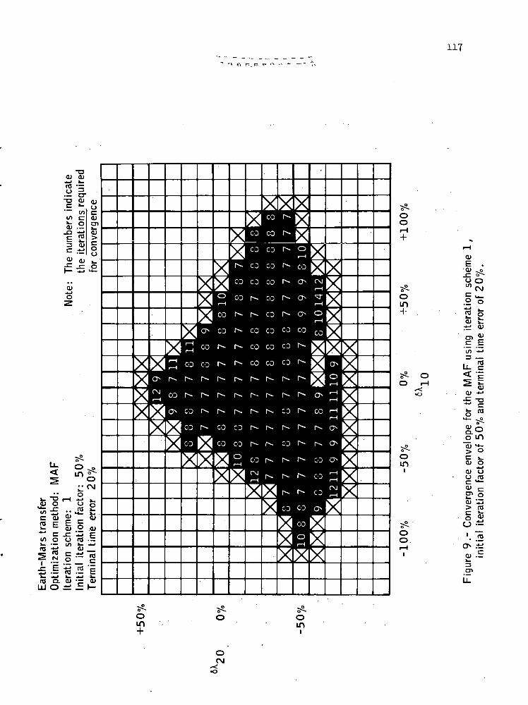
117
OOi-H
Oin
oo
00" Cxic ,.2 o
1*01 t
™ <DOi -
E .§(/I 'j_>
"re
MO) -»J
_o"mO) <*r> OC i_OJ O
4_*o> uoj5
s°01 U3> re
o •-I "m
O..E=3O>
Om
om
oC\J

118
positive terminal error is increased. This seems reasonable
since a negative X2o error, which decreases the initial control
angle, combined with a positive tf error would probably cause
the vehicle to intercept Mar's orbit at a low angle. This tra-
jectory would conceivably terminate closer, to the optimal point
than if the time error were less. " -
Figures 7, 8, and 9 also display the characteristic that
the envelope boundary becomes poorly defined, i.e., more irregu-
lar. This emphasizes the fact that-many 'times- only a slight
numerical difference exists between convergence and divergence',
and hence the scheme becomes very unpredictable near the bound-
aries. This is emphasized further by noting that in many cases
a divergence occurs, immediately after a. relatively low iteration
convergence case. .-—-•.•• •
Iteration Scheme 2 continues' to integrate the differen-
tial equations forward and skips the adjoint equation integration
unless a divergence occurs or a specified number (updating inte-
ger) of forward passes have been made. Figures 10, 11, and 12
show Iteration Scheme 2 for an initial iteration factor of 50
percent an.d updating integers of 2, ^, and 6, respectively. The
figures indicate the total iterations and the number of adjoint
integrations -required. Figure 8, showing Iteration-Scheme 1 ,•
may be considered a special case of Iteration Scheme 2 where the
updating integer is unity. A comparison of these figures reveals
that no significant change in the convergence envelope size or
shape has resulted from the application of Iteration Scheme 2 or
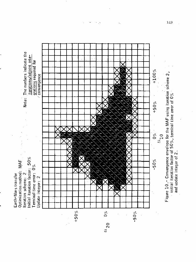
119
(U
-i «' .2 E- - - -re a. ai •— <i» a.
LJ O ±i ^ I—
OOi-H
Om
CM
(U
. o10c
O)
;-?. (—> »_ o
° £ "*o Jir ^^o O
Oin
_
g 2VJ <J
5 vS
rviC\J
*0
Si .2S1
i a— Q.
O .5 3
<u .E re01
oin
oCM

120
O)
Oo
oLT)
Oin
Oin
om
re
"^ ocvj "~aj. sj>
<u "co min ^
QJ c:
.E o31*-3 o
U. j-< £^ *>a> aj
o —**- re<u .50. r;
a> oginOJ u_CT> b
1°5 o<3J5
cI O, 4-J
i— i rei ^• a>
QJ ±i
O1
oC\J

121
ooi-H
Oin
EO» T3
JC C
00'*J >*-n ov >•4-1 O•— ^Oi O)
< «2-
cu
OIDl
O)
o s^
Kis<u o
C C xO<U O „_o^ ^» oo3 2 >-> QJ <"C *-" OlO — 0)
— <u5«
Q.<u'c\j^ _

122
increasing the updating integer. The total number of iterations
required increased, but the number of adjoint integrations de-
crease as the updating integer is increased. This trend con-
tinues until the updating integer reaches four or six and this
appears to be a point of diminishing return for this particular
problem. • . • .
It becomes apparent that the initial value of the itera-
tion factor has a pronounced effect on the convergence envelope
size, and in most cases convergence time as well. An initial
value of iteration factor of 20 percent, with either iteration
scheme, produces a significantly larger envelope than the ones
for 50 percent shown in Figures 7 through 12. This increase in
envelope size is accompanied by a significant increase in the re-
quired computer convergence time for Iteration Scheme 1. Figure
13 Illustrates this influence' of the initial values of iteration
factor on the convergence time for the particular but 'represen-
tative cases where the Lagrange multiplier and terminal time
errors are as indicated on the figure. For Case 1, where the two
Lagrange multipliers and terminal time errors are -10, -10, and
20 percent, respectively, the largest values of initial iteration
factor result in the most favorable convergence times. On the
other hand, for the case where the initial error is larger, as
Illustrated by Case 2 where the Lagrange multipliers and terminal
time errors are -20, 10, and 20 percent, respectively, some inter-
mediate value of Initial iteration factor results in the most
favorable time.
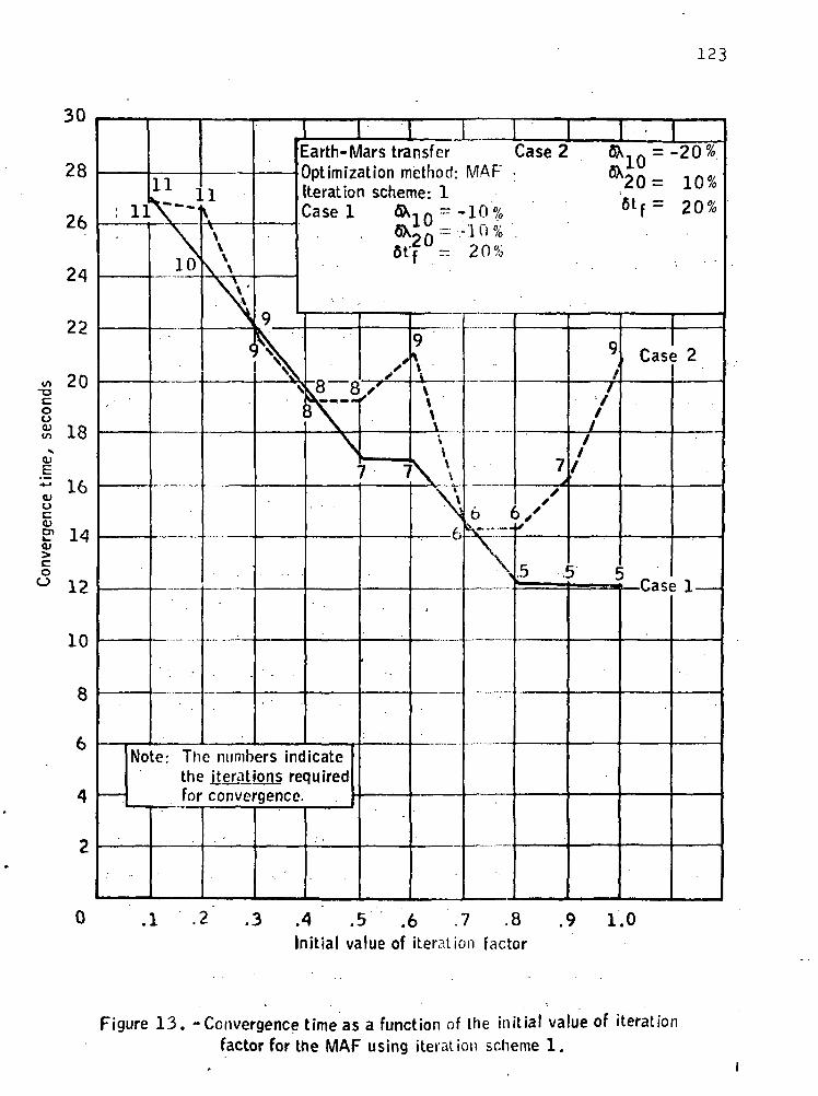
123
30
28
26
22
20
18
E
- 16<uocoE1 1401
coo 12
10
8
; 11
'
No
11 -
10
1
N\
^<
1
.9
\V
te: The numbers incthe Iterations refor convergence
IEarth- Mars traDptimization mIteration scherCase 1 6X
6X6t
JB 8\._,_.8\\
licatcquired
,'
•^— — _7 1
•
nsferethod:ne: 1
20 ~ 'r ~:
9\
V
\\\\
\\
A
•
Case 2 6X.Q = -20*.MAP" . fiXz;; ,nwe.\j — J.U /o
10% 6 t f= 20%
20%
4..J\
7s
3 /'
*
5 :.> .
9
- ^
/
/
>' _J
Cast
i — Casi
5 2
1 1
.1 .2 .3 .4 .5 .6 .7 .8Initial value of iteration factor
.9 1.0
Figure 13. -Convergence time as a function of the initial value of iterationfactor for the MAP using iteration scheme 1.

Figure 13 also reveals the existence of an uncertainty
about the selection of the initial iteration factor. When a
problem is first attacked, one has little or no feel for e per-
centage correction to request. A low initial value for the iter-
ation factor is usually selected because it is expected that this
results in a large envelope of convergence. A low initial itera-
tion factor results in a convergence time penalty as shown in
Figure 13. However, in some situations a high value for the
initial iteration factor results in a convergence time penalty.
It is not known how to determine the best initial iteration
factor before a series of investigations is made.
Iteration Scheme 2 attempts to overcome this problem by
seeking the largest iteration factor that can be used, without a
trajectory divergence, before the time consuming adjoint inte-
gration is ir.ade. Since only forward integrations are made in
bringing the iteration factor from a low Initial value'to the
beet value, the time penalty is reduced. The influence of ini-
tial iteration factor on the convergence time is illustrated in
Figure 1*4 for Iteration Scheme 2. This .plot may be compared to
one of the cases in Figure 13, and it is easily seen that for low
i-nitial values of the iteration factor the time penalty is not so
severe. The objection to an initial low iteration factor is re-
moved now, and yet good convergence possibilities remain because
large envelopes of convergence are associated with low initial
iteration factors.
The influence of the update integer on convergence time?
is illustrated in Figures 15, 16, 17, and 18. These envelopes

125
24
22
20
18
16inc
§ 14to
(U
.§ 12
o
en(U
coO
10
14,/313/3
\• .^
U/
11•*• •*•/
/2
/?'r £• -
10,
Note: The numbers indicatethe Iterations/adjointiterations requireconvergence
d for
/V/2
Earth-Mars transferOptimization method : MAFIteration schUpdate inkeg<Case 1 6\,
]OAp
6
/3
NN
T T11
/s
erne :if : 6
LO
0 ="tf = ;
/3 11
2
10%
10%
20%
/3
1 01U,/^f .>
.1 .2 .3 .4 .5 .6 .7 .8 .9 1.0
Initial value of iteration factor
Figure 14. - Convergence t ime as a function of the in i t ia l value of iterationfactor for the MAF using iteration scheme 2.

Earth-Mars transferOptimization method: MAPIteration scheme: 1 and 2Initial iteration factor: 50%Terminal time error: 0%Update integer: 1
126
+50%
20 0%
-50%
32 1 9 l:i 17 1 51
2 4 19 191;; i6 1 6 1 6 1 5 1 5 1 5O i » ) I O 10
,19 111 16 16 1616 16 2 1 5 1 5 I 7 i v |
^1715 1 5 1 5 1 5 1 5 1 5 1 5 1 5 1 6 1 5 1 5 1^19 15 15 15 15 15 15 15 15 i;; i ; ; i ; :
12 3 ! 9 1 7 1 5 1 5 1 5 1 5 1 5 1 5
-50% +50%
6 X 10
Note: The numbers indicatethe time in secondsrequired for convergence
Figure 15.- Convergence envelope, for the MAP using iteration schemes 1 and 2iteration factor of 50%, terminal time error of 0"/0 and update integer of 1 .
initial
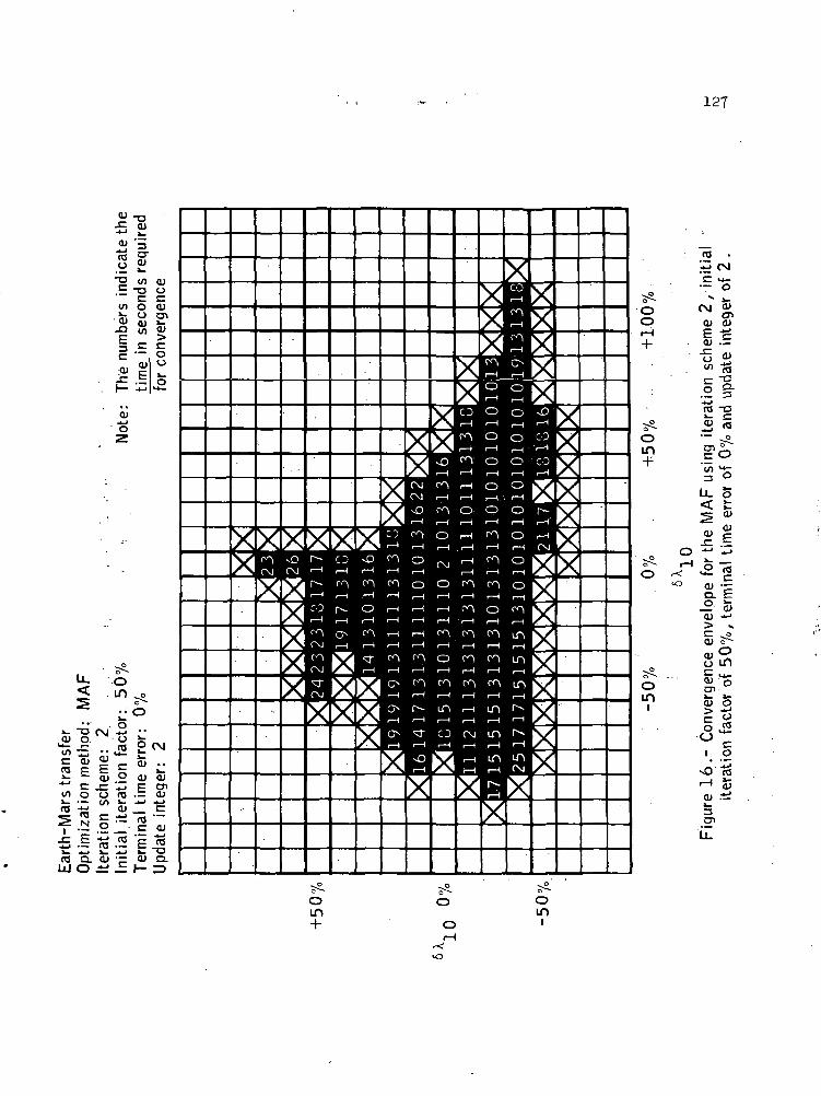
127
C\j <U
Q> d)
E cQJ .=
£- -O
I *"re -o»- c
^ re
"> ^=s ou. 5
?l
£ "reQJ •-Q. £
-° 5CU *-•
c ?Q> o^
<u°o u")
1°o3 o£ «0 <20 c
1 O
.^•'•5
301

128
0)
rO O- OJUl O ±i
CVJ<U
OJ
O -D(/> c
°
=3 O)
i_ O)
> u-C O
<L> Ui u—CT* _ O
|.2 85c •£ cr>o S «
CJ OJ c| '*"
r^ 5 "Jo__i *-» -n• c Q-OJ •- 3

129
re<D
re
E vOQJ u_
C 01O CL>
OJ OJ
11LL. re
s*So_c *ofe o
fcQ. O)
— .§
> ^
(U 'c
g|CTI
OIT*
oini
oo 5i t5
<u JS
oC\J

130
correspond to the envelopes in Figures 8, 10, 11, and 12, but
indicate the convergence times rather than the required Itera-
tions. A most interesting characteristic of Iteration Scheme 2
is revealed. For a given initial iteration factor of 50 percent,
the convergence times are generally reduced by increasing the up-
dating integer to the four to six range. Larger values of the
updating integer result in higher convergence times. It is ex-
pected that for thir, problem the best update integer approxi-
mately equals the number of steps required between the initial
value of the iteration factor and unity.
It is very interesting to take a specific and repre-
sentative example, and examine the norm of the terminal con-
straints as a function of computation time. Figure 19 shows the
terminal dissatisfaction norm decreasing for Iteration Scheme 1
for initial values of the iteration factor of 20, 50, 70, and 100
percent. Not only is the increase in convergence time for the
smaller iteration factors evident, but the characteristics of the-
convergence rate are also seen. Figure 20 illustrates these sarrc-
characteristics for Iteration Scheme 2 using an initial itcratior.
factor of 50 percent. The norm of the terminal dissatisfaction
is plotted as a function of computation time for update integf-rr-
of 1, 2, i), and 6. With an update integer of six, the conver-
gence time is approximately reduced by 50 percent when compared
to the extreme case where the integer is unity.
In an effort to determine some of the complications
associated with solving a different problem, the atmospheric

10
Earth-Mars transferOptimization method: MAPIteration scheme: 1Case: & in= 10%
<*— = 101%
fit, = 20%
Note: Percentages shownare the initial valuesof iteration factor.
131
10
i O-710 15 20Computation time, seconds
Figure 19. - Norm of terminal constraints as a function of computation timefor the MAP using iteration scheme 1.

132
Ul
"c're
o•o
O
EL.o
10
10-6
Earth-Mars transferOptimization method :Iteration, scheme : 2Initial Iteration factor!Case 6A10 = -10%
6X20 =-10%
6tf = 20%
MAP
: 50
Note: Numbers shown'arevalues of the updateinteger.
0 5 10 15 20 25Computation time, seconds
Figure 20. - Norm of terminal constraints as a function of computation timefor the MAP using iteration scheme 2.
30

133
Earth launch to circular orbit described in Appendix A.2 was
formulated and solved. These results are shown in Figures 21,
22, and 23. It was discovered, for the Earth launch problem,
that the convergence envelopes were less sensitive to terminal
time errors than for the Earth-Mars transfer. Hence, the plots
shown are the same as for previous cases with the exception that
terminal time variations are only 10 percent.
It is obvious from the figures that the method is rela-
tively sensitive to XJQ errors and relatively insensitive to
X2o errors. This Earth launch example reveals some of the same
characteristics seen for the Earth-Mars transfer, namely, as the
terminal time error increases the convergence envelope increases
in size and moves downward. This downward movement means a re-
duction of negative X2 error sensitivity.'4 .
One interesting characteristic, not seen in the Earth-
Mars transfer example, is that when the A2o error is 100 per-
cent, considerable convergence difficulty is experienced. This
case corresponds to the initial control angle of 90 degrees. It
is rather remarkable that convergence still results for some
cases where the initial control angle is greater than 90 degrees.
In summary, for Iteration Scheme. 1 the envelope of con-
vergence increases with positive increases in terminal time
error, for a given Initial iteration factor. The envelope size
is increased further with a reduction of initial iteration fac-
tor, but unfortunately the convergence time is increased. The
convergence envelope for Iteration Scheme 2 is also increased by
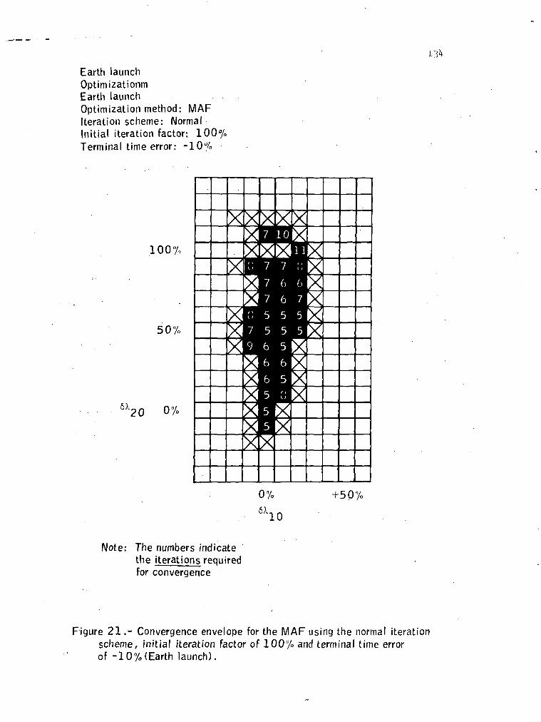
Earth launchOptimizationmEarth launchOptimization method: MAPIteration scheme: NormalInitial iteration factor: 100%Terminal time error: -I0u/o
100%
50%
X20 0%
0%
6\
+50%
10
Note: The numbers indicatethe iterations requiredfor convergence
Figure 21.- Convergence envelope for the MAP using the normal iterationscheme, initial iteration factor of 100'/o and terminal time errorof -10%(Earth launch).

Earth launchOptimization method: MAPIteration scheme: NormalInitial iteration factor: 100%Terminal time error: 0%
135
100%
50%
6X 20 0%
-50%
HJ7 7 60
S7 6 7!S!B<> 7 7®I*6 6 fe!BI
HUB* • SBG G 7 6 6 gg
g3(6 6 6 6 6g|
HJ6 6 5 7 5JQSl9 6 6 5 7gg
7 5 1
-50%
Note: The numbers indicatethe iterations requiredfor convergence
0%ixio
50%
Figure 22 .-Convergence envelope for the MAP using the normal iterationscheme/ initial iteration factor of 100% and terminal time error of 0%(Earth launch).

-150%
-100%
-50%
'^20 0%
-50%
-100%
-150%
136
Earth launchOptimization method: MAPIteration scheme: NormalInitial iteration factor: 100%Terminal time error: 10%
Note: The numbers indicatethe iterations requiredfor convergence
-100
Figure 23.- Convergence envelope for the MAP using the normal iterationscheme, initial iteration factor of 100% and terminaltime error of 10% (Earth launch).

137
reducing the initial iteration factor, for a given update inte-
ger. For a given initial iteration factor, the convergence time
is reduced by increasing the update integer. The best times re-
sult for update integers of approximately six, and increased
times result for further increases in the integer.
The significant fact is that Iteration Scheme 2 is
superior to Iteration Scheme 1 because low, and hence safe, ini-
tial values of the iteration factor may be used without resulting
in an unreasonably large convergence time.
The application of this optimization method to a differ-
ent problem resulted in approximately the same general conver-
gence characteristics.
6 3.2 Method of Perturbation Functions '
The required formulation as discussed in Section 3-2 is
simple and straightforward, and even more natural than MAP since
the perturbation equations are used directly. A general dis-
cussion of the applications is presented in Appendix A.2 and a
specific application or the MPF is made in Appendix A.2.2.
The programming effort requires the forward integration
of the eight differential equations, of motion and the Euler
differential equations. The eight perturbation equations must
also be integrated forward, and this must be done with three
different starting vectors. The coefficients for these pertur-
bation equations may be formed as needed and no storage is re-
quired. This represents a decided advantage over the MAP,

138
especially when the problem is of large dimension, because the
back spacing of'tapes is not necessary. The programming com-
plexity is reduced also because no checks are required for the
acquisition of proper coefficients, i.e., the coefficients are
simply formed as the forward integration is made. It may also
be.noted that one less integration Is required for the MPF as
opposed to the MAP, and this results in less total integration
time.
The integration of the perturbation equations requires
a large percentage of the total computational time. It is con-
ceivable that the same numerical accuracy might result when a
variable integration step size is used, however, this increases
the programming complexity considerably. A constant step size
was selected for the integration of all equations.
The computer program that uses the MPF requires two
initially assumed Lagrange'multipliers and an assumed'terminal
time. These-estimates require a familiarity with the physical
problem and, to some degree, experience. The computer program
is built such that only the subroutines containing the differ-
ential equations of motion, the Euler-Lagrange equations, and the
perturbation equations must be changed to solve different prob-
lems, and the effort is comparable to that required for the MAF.
Iteration Scheme 1 requires very little computer logic
in addition to the Normal Scheme of requesting 100 percent termi-
nal constraint satisfaction on each iteration. Operation is
simply transferred to a subroutine where the iteration factor is

139
altered in accordance with the terminal norm criteria explained
in Section 3.3- The process is essentially the same as that for
the MAP.
Iteration Scheme 2 requires some additional programing
and storage, and is comparable to that required for the MAP.
Basically, the scheme is such that the iteration factor is in-
creased, omitting a perturbation integration,, until either the
norm of the terminal constraints diverges or a 'specified number
of nominals have been generated. If the norm diverges, the last
convergent trajectory is used as a nominal, and hence this tra-
jectory must be saved until it, is determined whether or not it
will be needed. The storage problem can be eliminated by simply
regenerating the last convergent trajectory.
An extensive,.analysis of the MPF is not made since the
theoretical development in Section 3.2 shows that exactly the
same algebraic, equation used for the MAP is used to determine the
corrections. The only difference between the MAP and MPF is that
one less integration is required for MPF, and therefore a re-
duced convergence time is expected. The envelopes of convergence
for Iteration Scheme 1 using initial iteration factors of 100
and 50 percent, respectively, are shown'in Figures 24 and
25. The obvious fact is that the envelopes have the same size
and shape as the corresponding envelopes for the MAP shown in
Figures 5 and_8, and the numbers on the figures indicate an
equal number of iterations are required. Figures 26 and 27
Illustrate the convergence times for the above cases. A

Earth-Mars transferOptimization method: MPFIteration scheme: 1Initial iteration factor: 100%Terminal time error: 0%
+50%
V20 0%
-50%
-50% 0%X10
+50%
Note: The numbers indicate theiterations required forconvergence
Figure 24 .- Convergence envelope for the MPF using iteration scheme 1,initial iteration factor of 100% and terminal time error of 0%.

lUl
Earth-Mars transferOptimization method: MPFIteration scheme: 1Initial iteration factor: 50%Terminal time error: 0%
+50%
S10 7 8 ******
***** *J *n*9 8 8 1 0 9 8 *
0%
-50%
8 7 8 7 9
_ 1 0 8 8 8 7 7 7 7 9 1 0jgjlO 9 8 7 7 7 7 7 7 7 7****
1 9 8 7 7 7 7 7 1 7 7 8 9 W R^ 1 8 7 7 7 7 7 7 7 7 7 7 7 7 1^ 9 7 7 7 7 7 7 7 7 8 8 8 7 8 8
**** 9
7 7 7 7 7 7
-100% -50% 0%6X
+50%
10
Note: The numbers indicate theIterations required forconvergence
Figure 25.- Convergence envelope for the MPF using iteration scheme 1,initial iteration factor of 50% and terminal time error of 0%.

Earth-Mars transferOptimization method: MPFIteration scheme: 1Initial iteration factor: 100%Terminal time error: 0%
+50%
^20 0%
-50%
Note: The numbers indicatethe time in secondsrequired for convergence
Figure 26.- Convergence envelope for the MPF using iteration scheme 1,initial iteration factor of 100% and terminal time error of 0%.

Earth-Mars transferOptimization method: MPFIteration scheme: 1Initial iteration factor: 50%Terminal time error: 0%
+50%
0%
-50%
^ *£330161515 131603
|Q@J2 0 1 6 1 3 1 5 1 3 1 6 2 3gj
(g(2 0 1 6 1 6 1 6 1 3 1 3 1 3 1 3 1 6 2 OJ^j
201 ; ; 16 1413131313131313^|^|g3g3
^117151313131313 2 13131516^88'1513131313131313131313131319
1613131313131
-100% -50% 0% +50%
6\10
Note: The numbers indicatethe time in secondsrequired for convergence
Figure 27.- Convergence envelope for the MPF using iteration scheme 1, initialiteration factor of'50% and terminal time error of 0%.

comparison of the convergence times may be made between the MAP
and MPF by comparing the times shown in Figures 15 and 27, re-
spectively. It is seen that the MAF must integrate a comparable
set of differential equations four times rather than only three,
as required by the MPF. Iteration Scheme 2 for the MPF war> not
programmed. •
The significant fact is that the MPF results in the
same envelope of convergence and requires.-the same number of
iterations as the MAP, but approximately 20 percent less com-
puter time is required because one less integration is needed'.
6 . Jl Quasilincarization Methods
The comparison and discus.sion of'the- Quasilinearization
Methods will cons'ist of. two separate analyses. The Method of.
Generalized Newt-.on-Raph'sbn', '--i-ncludirig'-^the normal procedure and
Iteration S'c.lYeme. 1 is discussed first. The Modified Quasilinear-
ization Method including the normal procedure and Iteration
Scheme 2 is discussed last. The Modified Method of Generalized
Newton-Raphson is also discussed briefly, but the MQM is empha-
sized. The discussion content will include the applicable items
listed in the Section 6.2.
6.^.1 Method of Generalized Newton-Raphson
The required formulation of the Method of Generalized
Newton-Raphson as discussed in Section 4.1 is simple and rela-
tively easy to apply, although this particular method is not

capable of handling terminal constraint functions or determining
the terminal time in an efficient manner. For these reasons, an
extensive investigation of this method is not made. However,
several runs are made, and spot comparisons illustrate its effec-
tiveness with respect to the other methods.
The programming effort requires the forward integratiorr
of the homogeneous parts of eight linearized differential equa-
tions of motion and the Euler differential equations. Also the
nonhomogeneous parts are integrated forv/ard once, and all coeffi-
cients for the solution of a linear system must be included for
use after each trajectory iteration. When convergence is ob-
tained for the specified value of terminal time, a time iteration
is made by making a scalar application of the Newton-Raphson
technique.
If the solutions to both the homogeneous and nonhomo-
geneous equations are stored, a new nominal is immediately avail-
able. However, to conserve storage only the terminal values of
the solutions are stored and the next nominal is simply generated
by an additional integration.
The current trajectory is generated from the preceding
trajectory, however, after a positive correction of terminal time-
has been made, no previous information is available. This fact
represents a problem that does not exist for the MAP or MPF. The
program is written so that a linear extension of all the varia-
bles of the pre-vious nominal is made to provide information for

116
the current trajectory.
The computer program that uses the MGNR requires two
initially, assumed Lagrange multipliers, an assumed terminal time,
and an initial trial solution consisting of the time histories of
all eight variables. The estimates require a familiarity with
the physical problem to insure that the assumed quantities' are
close enough to optimal that convergence will result. The sig-
nificant difference between MGNR and MAF or MPF is that a com-
plete solution must be assumed rather than Just initial starting
values of the variables. If no reasonable solution can be de-
cided upon, the nonlinear equations may be integrated to provide
the first solution. However, in the more complex problems, this
solution may not be adequate to result in convergence.
The program is built such that only the subroutines con-
taining the nonhomogeneous and homogeneous equations and the
trial solution must be changed to solve different problems. A
constant integration step size was selected for all integrations.
The Normal Scheme of the MGNR is that of making tra-
jectory Iterations, requesting 100 percent correction in the
terminal constraints, until convergence results for the assumed
terminal time. Then a time iteration is made and the process
continued. Iteration Scheme 1 requires very little additional
computer logic. This scheme amounts to avoiding time iterations
until the present metric becomes less than the previous metric.
The logic is simply inserted in the program, and an additional
subroutine is not used.

A typical example of the convergence characteristics of
the MGNR is shown in Figure 28. This illustration shows how the
metric decreases as a function of computation time for the case
where the Lagrange multipliers and terminal time errors are -10,
-10, and 20 percent, respectively. A linear initial trial solu-
tion is used and this solution is represented by long dashed
lines in Figure A.2.1. Trajectory iterations are made until the_s
metric is less than. 10 , then a time iteration is made. During
the initial stages, the time iteration essentially destroys the
reduced'metric that has just been.obtained. This characteristic
is not quite so severe when terminal time errors are small.
The convergence characteristics for the same example,
using Iteration Scheme 1 are shown, in Figure 29, and a signifi-
cant reduction in computation time is evident. This scheme
appears superior to the normal procedure, but it must be pointed
out that a theoretical analysis of this scheme has not-been made
tO'define a bounds for convergence. For a given terminal time,
the convergence proof given by McGill (14) applies, but' the time
iterations could be so poor that divergence would result. The
examples in Figures 28 and 29 show that the Iteration Scheme 1
results In a convergence time that is 43 percent less than that
required by the Normal Scheme.
The Modified Method of Generalized Newton-Raphson, dis-
cussed In Section 4.1, Is modified in the sense that a change in
the independent variable Is made to eliminate the cumbersome de-
termination of terminal time. One advantage of this .method is

10
a>
Earth-Mars transferOptimization method: MGNRIteration ischeme: NormalInitial solution: Linear
5X in = -10%= -10%
10
10
10-6
20 30 40Computation time, seconds
Figure 28. - Metric p as a function of computation time for the MGNRusing the normal iteration scheme.
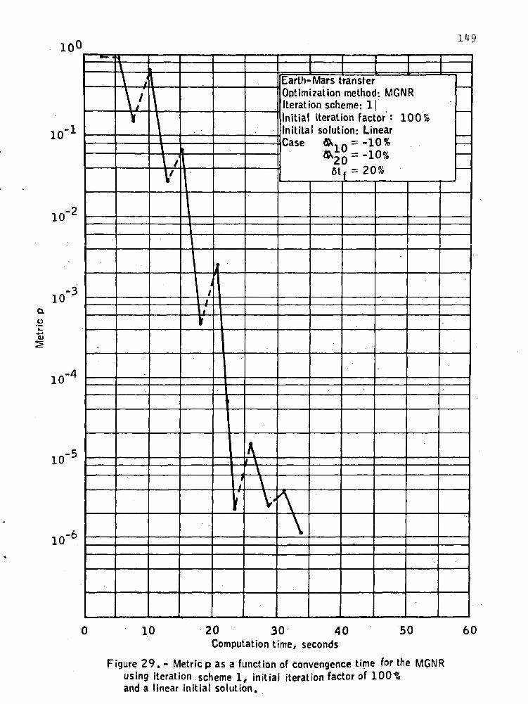
a>
10°149
Earth-Mars transferOptimization method: MGNRIteration scheme: Ijinitial iteration factor : 100'Initital solution: LinearCase 6V =
6tf = 20%
10 20 30 40Computation time, seconds
50 60
Figure 29. - Metricp as a function of convengence time for the MGNRusing iteration scheme 1, initial iteration factor of 100"%and a linear initial solution.

150
that the independent variable range is the same for all itera-
tions, thus simplifying the programming slightly. A disadvantage
is that one additional equation must be Integrated and a rather
complex term is added to each of the existing equations. The
most significant advantage is that the terminal time determina-
tion becomes an integral part of the-iteration process.
The convergence characteristics of the MMGNR is illus- •
trated in Figure 30 for the same case shown in Figures 28 and 29
for the Normal Scheme and Iteration Scheme 1, respectively, using
the MGNR. The metric reduction becomes a monotonic function of
computation time, and when a linear initial solution is used the
convergence time is 27 percent less than that required by the
MGNR using the Normal Scheme. Figure 30 also shows the conver-
gence characteristics for the case where the initial trial solu-
tion is determined from integrating the nonlinear differential
equations.
6;*4.2 Modified Quasllinearizatlon Method
The required formulation of the Modified Quasilineari-
zation Method as discussed in Appendix A.2.3 is simple and rela-
tively easy to apply and this method is capable of handling
terminal constraint functions. The terminal time determination
is included as an integral part of the process and this method is
very efficient compared to the MGNR. Also, no additional equa-
tions or terms are needed as with the MMGNR.
The programming effort requires the forward integration

10'
10-1
10-2
10-3
Q.o
10-4
10-5
10-6
\N151
. \
Linear
Earth^Mars transferOptimization method: MMGNRIteration scheme: NormalInitial solution: Nonlinear and LinearCase ft.Q='-iO%
»• w6t f: =
.Nonlinear
-V
*V
5 10 15 20 25Computation time, seconds
Figure 30. - Metric p as a function of computation time for the MMGNRusing the normal iteration scheme.
30

152
of the homogeneous parts of eight linearized differential equa-
tions and Euler-Lagrange equations. Also, 'the nonhomogeneous
parts are integrated forward and all coefficients are evaluated
from the previous nominal. The corrections that must be applied
for the next iteration are determined by solving a linear system.
Only the terminal values of the forward integrations are stored
as explained in Section .6.4'. 1. When a positive terminal correc-
tion is made, a linear extension of the variables from the pre-
vious nominal is made.
The computer program that uses the MQM requires two ini-
tially assumed Lagrange multipliers, an assumed terminal time,
and an' initial trial solution. In a manner similar to the MGNR,
if a reasonable initial solution cannot be selected, the non-
linear equations may be integrated to provide an initial solu-
tion. The program is built such that only the subroutines con-
taining the nonhomogeneous and homogeneous equations and the
trial solution must be changed to solve different problems.
The Normal Scheme of the MQM is that of requesting a 100
percent correction in the terminal constraints. Iteration Scheme
2, used with the MQM, is similar to Iteration Scheme 1 for the
MAP or MPF, where a percentage- correction in the terminal con-
straints is requested. The logic required to determine whether
the iteration factor is increased or decreased in the Quasi-
linearization Methods is more complex than that required for the
MAP or MPF., because .the metric p must be determined. This cal-
culation requires several operations on all eight dependent

11)3
variables at each time step and hence requires a relatively large
amount of time compared to the calculation of the norm in the MAP
or MPF.
The convergence envelopes for the MQM using the Normal
Scheme, a nonlinear initial trial solution and -20, 0, and 20
percent errors in terminal time, respectively, are shown in
Figures 31, 32, and 33- The nonlinear initial trial solution is
the one that results from integrating the nonlinear differential
equations. Comparing these Figures with the Figures 1, 2, and 3
for the MAF reveals that while the general shape of the envelopes
are the same, the MQM results in slightly smaller envelopes. For
negative and zero terminal time errors, the method is extremely
sensitive to Lagrange multiplier errors that have the same sign.
For positive terminal time errors, the method is much more sen-
sitive to positive \2 errors than to negative X2 errors.
An attempt to generate the same envelopes by using the
MQM with a constant initial trial solution must be recorded as a
failure, because no convergent solutions were obtained. The con-
stant initial trial solution used is illustrated in Figure A.2.1
by short dashed lines.
Figures 3^ , 35, and 36 illustrate the convergence en-
velopes for MQM using Iteration Scheme 2 with an initial itera-
tion factor of 50 percent, a nonlinear initial solution and -20,
0, and 20 percent errors in terminal time, respectively. These
envelopes.are significantly larger than the envelopes for the
Normal Scheme shown In Figures 31, 32, and 33. It Is interesting

Earth-Mars transferOptimization method: MQMIteration scheme: NormalInitial iteration factor: 100%Terminal time error: -10%Initial solution: Nonlinear
+50%
0%
'20
-50%
-50%
Note: The numbers indicatethe iterations requiredfor convergence
50%
Figure 31.- Convergence envelope for the MQM using the normal iterationscheme, initial iteration factor of 100% and terminal timeerror o f -20%.

155
Earth-Mars transferOptimization method: MQMIteration scheme: NormalInitial iteration factor: 100%Terminal time error: 0%Initial solution: Nonlinear
+50%
6X20 0%
-50%
.-50% 0%
6X
+50%
10
Note: The numbers indicatethe iterations requiredfor convergence
Figure 32 .- Convergence envelope for the MQM using the normaliteration scheme/ initial iteration factor of 100%and terminal time error of 0%.

Earth-Mars transferOptimization method: MQMIteration scheme: NormalInitial iteration factor: 100%Terminal time error: 20%Initial solution: Nonlinear
156
50%
.~.20;
"vl
9 7 6 6 6 C 12
G 9 1010 9 9 G G
,.JL.
0%
<' - •
Note: The numbers indicatethe iterations requiredfor convergence
Figure 33.- Convergence envelope,for the MQM u-si,ng!the.,nprrnal|jiterationscheme, initial iteration factor of 100% and terminal,time error of 20%

157
Earth-Mars transferOptimization method: MQMIteration scheme: 2Initial iteration factor: 50%Terminal time error: -20%Initial solution: Nonlinear
+100%
+50%
6\200%
-50/o
-100% -50%
Note: The numbers indicatethe iterations requiredfor convergence
0%>X10
+50%
Figure 34.- Convergence envelope for the MQM using iteration scheme 2,initial iteration factor of 50% and terminal time error of -20%.

158
<v <u
.- o-•o <u m
.E •- o
<u <-QE3C ;
OJ a,
Ol.4-1o
o>
Iou
fe
"O CM.0
0 JSin ^o gE
fe 1" f e z« 2 z
re
re
<L>c ^:o o
c:o
IIO. <1>O ±i
co c
O) Oii C^ .«-»
2.= o
re «n
«
CNJ
ai
o</>
en
.ssO) O)
u— re
•a im> «_c o
<u o
II
QJ.E
3
\L
Om
Om
oC\J

159
CM
<U
tuo •<-o
™cu
01
. -ao 5«— reQJ -5
asE1 cO) O
i'l
01 =
CT1
L
re o. o»LU O ±i
Om
oinoC\J

160
to note that while the envelopes for the Normal Scheme are ,,
slightly smaller than the corresponding envelopes for the MAF,
the envelopes shown in Figures 3^> 35, and 36 are .slightly larger
than the corresponding envelopes for the MAF shown in Figures.?,
.8, and 9. This suggests that Iteration Scheme 2 for the Quasi-
linearization Methods is more effective than Iteration Scheme 1
for the Perturbation Methods. The Figures 3*4, 35, and 36 follow
the pattern previously mentioned for the other methods in that
the method is increasingly sensitive to positive *2 errors as
the terminal time error increases.
It is of definite interest to note the required conver-
.gence times for the cases illustrated for the MQM. As an ex-
ample, Figure 37 shows the convergence times for the envelope of
Figure 35. This envelope may be compared directly with the
corresponding envelopes generated by the MAF in Figures 15, 16,
17, and 18 and the MPF in Figure 27. An obvious fact is that the
MQM requires slightly more computation time than the MAF and MPF,
.but shows considerable improvement over previous quasilineari-
zation techniques such as the MGNR and MMGNR. In all fairness,
however, it must be pointed out that more time was spent in trying
to make the programming efficient for the MQM than for the MGNR
and MGNRM.
An insight to the convergence characteristics of the MQM
may be seen in Figure 38 for the special case where the Lagrange
multiplier and terminal time variations are -10, -10, and 20 per- .
cent, respectively. This figure may be compared directly with

161
OJuc
<U QJ•4-1 .- CTtm </> »-O -O QJ.- C >•O O CC O O— <l) (J
oj ='~cu
QJ3O"
J= QJ— »-
03.4-)O
0 fcm ^o S
Jr. "2 ™ -^ • • oQJ
O O•— en-s;s =_ o
c « cO a, o
E -< _ o.ti re to_ c _
re Q. QJ ••—
^TCM
•vT CMCM CM
O OCM CM
3—©—©-
vj CM CM
•xT OCM CMOCM
O OCM CM
CM O O O COg CM CM CM CM r—I• O O O O CO. CM CM CM CM i—(
i vD CM O CO CDCM CM CM r—I ,—i
'O O CO CO COCM CM
CO vO xQ COCM CM CM CM
CO CO Or—I r—I CM
<T ° °^ CM CM
CO O Or-1 CM CMCO O O^H CM CM
CO O Or—I CM CM
CO O O! i—I CM CM
O CM OCM CM CM
vT CM O( S CM_ CM
CM OCM CM
.. CM ™
^r cr ^rCM CM ^
O CMCM CM
O CCM CM
-©—©-CM CM ,
O CM CMCM CM C^
O CM rCM CM |O CMCM CMO OCM CMO CMCM CMO <vTCM CMo ^rCM CM
O *Q 'CM CM
O .£>CM CM
O vOCM CM
O ;;CM CM '
oin
Co-
£OJ
re•4-f
'c
QJ
OffiCO
O |
<o
•c
i:QJ
O
m
oo
»_ 0)£ QJ
sic -aQJ cai re^QJ --?
Om o
C\J
om

162
aoh_4_*flj
Earth-Mars transferOptimization method: MQMIteration scheme: 2Initial iteration factor; 100%Initial solution: Nonlinear
10
.,10 15 20Computation time, seconds
Figure 38. - Metric p as a function of computation time for the MQMusing iteration scheme 2, and initial iteration factorof 100% .

163
Figures 28, 29, and 30 for the MGNR using the Normal Scheme,
MGNR using Iteration Scheme 1 and MMGNR, respectively. Figure 38
may also be compared, in a sense, with the 100 percent curve in
Figure 19 for the MAF. Caution must be exercised, however, be-
cause the ordinates represent different quantities. It is ex-
pected that a reduction of the metric p is more stringent a re-
quirement than reduction of the terminal constraint norm. The
more stringent requirement results from the fact that the metric
p is composed of so much" more information than the terminal con-
straint norm.
Figure 39 illustrates the effect of the initial value of
iteration factor on convergence time for two specific cases of
Initial parameter error. This figure may be compared to Figure
13 which represents the same information for the MAF for the same
cases. The same characteristics are noted in that for some cases
the best initial iteration factor is somewhat less than 100 per-
cent and that this.best value Is not the same for all cases. One
additional characteristic, noted in Figure 39, is that very large
penalties in the convergence times are paid when low initial
iteration factors are used. This deficiency is attributed to the
metric criteria used to determine how the iteration factor must
be changed. When only a small percentage correction is re-
quested, the metric does not decrease rapidly at first. This is
because the metric is interpreted as the maximum distance between
successive trajectories. In fact, in application the metric
sometimes increases slightly and this causes the iteration factor

,16A_ ^-
en•a
oua>CO
ua>E1
OJ
coO
38
36
34
32
30
28
26
24
22
20
18
16
14
12
I I I I IEarth-Mars transfer -. •Optimization method: MQMIteration scheme: 2Initial solution: Nonlinear
ss-10 fl-
* 20%at
»20 = 10 %6tf =20%
Case 1 -11
10.
Note: The numbers indicatethe iterations, requiredfor convergence.
.1 .2 .3 .4 .5 .6 .7Initial value of iteration factor
.8 .9 1.0
Figure 39. - Convergence time as a function of the initial value ofiteration factor for the MQM using iteration scheme 2,
and a nonlinear initial solution.

165
to decrease. This process could conceivably have a decelerating
effect on the convergence. This phenomena may be seen in Figure
1*0 for the case where the initial iteration factor is 20 percent.
Figure 40 also illustrates the convergence characteris-
tics for several different initial iteration factors and may be
compared to Figure 19 which represents the same information for
the MAF for the same case. It should be noted that near the
terminal phase of each trial the metric reduction is nearly quad-
ratic.
In summary, the Quasilinearization Methods show a wide
range of convergence characteristics, but the proposed method,
the MQM, successfully reduces the convergence times and increases
the convergence envelopes to become competitive with the MAF and
MPF.
Generally speaking, the MQM displays the same character-
istics that are seen for the MAF and MPF. For the case when an
initial iteration factor of 50 percent is used, the envelope of
convergence for the MQM is slightly larger than the corresponding
envelope for the MAF and MPF. But the convergence times are al-
ways slightly larger than for the MAF.
6.5 Gradient Methods
The comparison and discussion of the Gradient Methods
will consist of two separate analyses. The Method of Steepest
Descent, including Iteration Schemes 1 and 2, is discussed first,
and the Modified Method of Steepest Descent is discussed last.

166
10°
d)
6tf = 20%
Percentages shownare the initial values
10-6
20 30 40Compulation time, seconds
Figure 40. - Metric p as a function of computation time for MQMusing iteration scheme 2 and a nonlinear initial solution.

. 167
The discussion content will include the applicable items listed
in Section 6.2.
6.5.1 Method of Steepest Descent
The required formulation of the Method of Steepest de-
scent as discussed in Section 5.1 is simple and straightforward,
but slightly cumbersome when compared to the MAP or MPF. A spe-
cific application of the MSD is presented in Appendix A.2.1.
The programming effort requires forward integration of
four differential equations of motion, storing the dependent
variables in computer memory or on tape at each time step. This
requires less storage than storing the A and B matrices. The
four adjoint differential equations, Eq. (5.6), are integrated
backwards five times using the variables stored during the for-
ward integration to form the coefficients. One additional com-
plexity is that Eqs. (5-30) through (5.32) must also be inte-
grated backwards, and may be carried along simultaneously with
the adjoint equations. To reduce the programming complexity, a
constant integration step is used for all integrations. The com-
puter storage problem can be eliminated by integrating the dif-
ferential equations of motion backward along with the adjoint
equations, Eq. (5.6), and Eqs. (5-30) through (5-32). This is
not done in the present method because the equations of motion
must be integrated forward anyway to determine the terminal
values of state.
In addition to the programming effort explained above,

168
the most serious disadvantage of the MSD is that a moderate
amount of human intervention and experience is required to im-
plement the program. For example, the weighting matrix W is
not defined, and by Just using the unity matrix the less sensi-
tive regions of the control program are very slow in acquiring
the optimal shape. The weighting matrix may be us.ed to speed
this optimal shaping process, but the insensitive regions of the
control program are not always known. , .
An examination of Eq. (5-33) reveals that the first
group of terms are related to the minimizing effort while the
last, group of terms are related .to the terminal constraint satis-
faction. .There is,, however, some cross coupling of the. terminal
constraint satisfaction in .the first term;.. The, procedure used to
affect convergence requires a selection of an .allowable average
control deviation, based on Eq. (5.19), that does not invalidate
the linearity constraints on the problem. This allowable control
deviation must be reduced in some specified manner as the process
progresses. If the numerator of the radical in Eq. (5.33) is
negative when 100 percent correction in the terminal dissatis-
faction is requested, the percent correction that causes the
radical term to vanish is determined. When this occurs, emphasis
is placed on reducing.the terminal dissatisfaction. If the
numerator is positive when 100 percent .correction is requested,
the radical is used and both the performance index is reduced,
and the terminal constraints are driven toward satisfaction. The
computer logic involved in the above operations requires a

169
significant amount of the iteration time.
The computer program that uses the MSD requires the ini-
tial value of the state variables, a stopping condition and an
assumed control program. These estimates require some familiar-
ity with the physical problem." The stopping condition that is.
chosen must be one that will be satisfied. The control program
selection is not as critical as it is for the MQM. The computer
program is not so easily generalized as it is for the MAP, MPF,.
or MQM, i.e., extensive programming is required to accommodate a
different problem. .
Iteration Scheme 1 simply uses the unity matrix for W •ft
and Iteration Scheme 2 .uses the H matrix. This second
scheme requires some additional computer storage and programming.
When Iteration Scheme 2 is to be used, H must be formed with
the variables that result from integrating the adjoint differen-
tial equations • backwards, using v as given in Eq.. (5'.27) for
the starting conditions. A major problem when using Iteration
Scheme 2 is that when a percentage correction in the terminal
constraints is requested, thereby forcing the radical term in
Eq. (5.33) to vanish, v becomes infinite. Clearly this cannot
be used as a starting condition for the adjoint equations.
With the examples discussed, this radical term vanishes
for the first few iterations, and when this happens the unity
weighting matrix is used. As soon as the radical becomes finite,it
the H matrix is calculated for use on the following tra-
jectory.

170
The thrust angle as a function .of mission time for the
Earth-Mars transfer is shown in Figures til, 42, -43, and 44, and
the convergence process from the assumed history, to .the. Eulerian
history is illustrated. Figures 41 and 42 show the convergence
characteristics for two widely" different initially assumed con-:
trol programs, designated Case 1 and Case 2, using Iteration
Scheme 1. 'It is interesting to note that the number of itera-
tions required is relatively independent of the initial control
program. After 30 iterations both cases yield control programs
that almost obscure large portions of the Eulerian program^- and
hence are not shown.. When to terminate the iteration process is
not clear since the Eulerian optimal is really never reached.
The method used here was to continue until'no further improvement
was being made, i.e.., until the solution began to oscillate about
some mean path. A more sophisticated .method would be to termi-Tnate when a time integral of H ; or H H became arbitrarily
small. • ' • : . -i. ..- v • • . . '
An apparent discontinuity begins to develop at approxi-
mately 100 days, as seen in Figure -1*1, and becomes more severe as
the iterations progress. After 30 iterations the apparent dis-
continuity becomes very sharp and the Eulerian control is accu-..
rately approximated.. The same characteristic is-noted in Figure
4 2 . • ' . • •
The-effectiveness of Iteration Scheme 2- in shaping the
optimal control program is Illustrated In Figures 43 and 44, and
it Is seen that the number of iterations required is signifi-
cantly reduced. In comparing Figures 41 and 43, for instance,

171
360
330
300
Note: The numbersindicate iterations
20 40 60 80 100 120 140 160 180 200 220
Mission time, days
Figure 41. - Thrust angle as a function of mission time for Earth-Mars transfer' using the MSO and weighting matrix W = I.
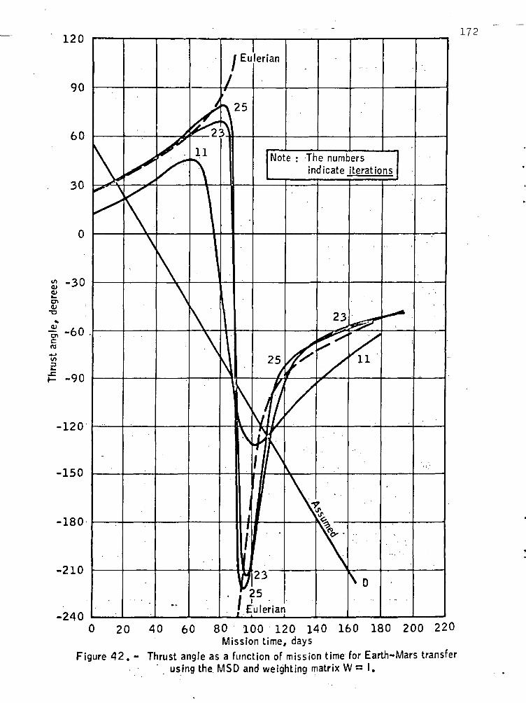
120
90
60
30
0
8 -300>
o>OJ
T3
1-60cro
-90
-120
-150
-180
-210
172
-240
Note : The numbersindicate iterations
0 20
Figure 42. -
80 100 120 140 160 180 200 220Mission time, days
Thrust angle as a function of mission time for Earth-Mars transferusing the MSD and weighting matrix W = I.

173
360
330
Note: The numbersindicate iterations
30
0 20 40 60 80 100 120 140 160 180 200 220
Mission time, days
Figure 43. - Thrust angle as a function of mission time for Earth-Mars transferusing the MSD and weighting matrix W = H.

174'
120
QJOJO41•o
JUcncre
Note: The numbersindicate Derations
-90
-120
-150
-180
-210
-24080 100 120 140 160 180 200 220
Mission time, days
Figure 44. - Thrust angle as a function of mission time for Earth-Mars transferusing the MSD and weighting matrix W= HUy.
175
it is seen that the apparent discontinuity development is much.
faster in the latter figure. These two cases are identical for
the first 11 iterations because the radical in Eq. (5.33) van-th *
ishes and W = i, but starting with the 12 iteration, the HUU
matrix is formed and used. It is during these final iterations
that the.full value of Iteration Scheme 2 becomes evident. After
only four additional iterations the apparent discontinuity, as
shown in Figure 13> is well beyond the development shown in
Figure ill. Moreover, the Eulerian is much better approximated,
for a given number of iterations, when Iteration Scheme 2 is
used.
The same characteristics are seen in Figures 42 and 44.« .
For this case, however, the H matrix is not calculated until
the 23r iteration. After only two additional iterations, Itera-
tion Scheme 2 in Figure 44 shows marked improvement in the devel-
opment of the apparent discontinuity.
An average Iteration for Iteration Scheme 1 requires
approximately 2.75 seconds of computer time, while approximately
3.0 seconds is required with Iteration Scheme 2 when the H
matrix must be formed. However, an extensive step size study was
not made for the MSD. The step size used was the same as that
used for the integrations in the indirect methods.
It should also be pointed out that the terminal con-
dition resulting from Eq. (2.14) may be used to determine the
terminal value of the Lagrange multipliers. These values are
used to start the backward integration of the adjoint equations,

176
for the H determination, and also may be used to estimate
the Lagrange multipliers required for starting the indirect opti-
mization methods. For the case illustrated in Figure 44 the
first time H, is determined, the values of Xin and. X2oUU . • ,
are calculated to be 2.15 and 0.65 percent larger than, the values
that correspond to the optimal trajectory, respectively. This
error is well within the envelope of convergence of all.the in-
direct methods studied.
6.5.2 Modified Method of Steepest Descent
The required formulation of the Modified Method of
Steepest Descent as discussed in Section 5.2 is simple and
straightforward, and is not as cumbersome as the MSD. A. spe- .
clfic application of the MMSD is presented in Appendix A.2.5-
The programming effort requires forward integration' oft
four differential equations of motion, storing the dependent
variables in computer memory or on tape at each time step. This
requires less storage than storing the A and B matrices. The
four adjoint differential equations are integrated backward only
once, using the variables stored during the forward integration.
The Eq. (5.48) must also be integrated so that after a desired
penalty function decrease is specified, a step size K may be
determined. The MMSD requires a significantly reduced number of
operations, as opposed to the MSD, because the adjoint equation
is integrated backwards with three less starting vectors and the
Integration of Eq. (5.^8) is much less time consuming than the

177
integration of Eqs. (5.30) through (5.32) in the MSD. The stor-
age problem associated with the first forward integration may be
avoided in a manner similar to that suggested in Section 6.5.1-
The present method does store the forward integration and use a
constant integration step size for all integrations.
In addition to the programming effort explained above,
the most serious disadvantage of the MMSD is that a considerable
amount of human intervention and experience is required to imple-
ment the program, even more than that required for the MSD. For
example, the step size K is not defined, and must be approxi-
mated by using Eq. (5. 8). A still more serious deficiency is
that a constraint on the control deviation is not included as an
integral part of the method itself, and hence appropriate com-
puter logic must be used to insure that the linear constraints of
the problem are not violated. One further complexity is that the
convergence characteristics are highly dependent on the factors
that weight the terminal constraints in the penalty function, and
the magnitude of these factors are not specified. To compound
the matter, the rates at which these factors are changed to
tighten the terminal constraints are not known. It is seen that
the price that must be paid for the simplicity of the method is
that of increased arbitrariness, and a considerable amount of
skill and experience is required to obtain meaningful results.
This method has been programmed and is in the stage of evalua-
tion, , butrno results are presented here.

178
6.6 Summary of the Comparison
The comparison of optimization methods thus far has con-
sisted of individual analysis of each method with an occasional
comment concerning the relative merits of one method with respect
to the others. It would be helpful to summarize the conclusions
of the comparison with particular emphasis on the basis of com-
parison as outlined in Section 6.2. A summary of the comparison
is:
(1) The programming complexity and required formulation
. , time is.greater for the MQM and MSD than for the MAP/
MPF and MMSD, because more computer logic is required.
(2) The MAP and MSD requires more computer storage than
the other methods.
(3) The MSD and. MMSD require more human intervention«
and intuition than the other methods, and hence are
difficult for inexperienced personnel to use. However,
.the indirect methods become difficult to implement -when
the problem dimension is large.
CO The computer program for the MSD requires consider-
able modification for solving a different problem, while -
the other programs require less modification.
(5) The convergence envelope sizes for all the indirect
methods are essentially the same when the initial itera-
tion factor Is near 100 percent. The MQM envelope is

179
slightly larger than the envelopes of the other methods
when the initial iteration factor is in the 50 percent
range.
(6) Th0e time penalty associated with the lower initial
Iteration factors is greater for the MQM than the other
indirect methods. ;
(7) The MPF is superior to the MAP and MQM when conver-
gence time is considered, because of the one less equa-
tion that must be integrated.
(8) The approximations to the Lagrange multiplier val-
ues as derived by the MSD are well within the conver-
gence envelopes of all the indirect method investigated.

CHAPTER 7
DESCRIPTION AND EVALUATION OF NUMERICAL PERFORMANCE
The evaluation of numerical performance is an essen-
tial feature in assessing the accuracy of an optimization
technique. The primary sources of error are encountered dur-
ing numerical integration and solving of linear systems
(which includes matrix inversion). Most of the computational
time is taken during numerical integration and hence, in-
creasing the speed of the integration will have a pronounced
effect on the total computer time. The criterion used for
defining convergence is also a factor in determining total
time, and if caution is not exercised an unrealistic com-
parison between different optimization methods could result.
7. 1 _ Numerical Integration
There are many characteristics that must be con-
sidered when selecting a particular numerical integration
sch'eme; some of the most important are accuracy, stability
and speed. The method and procedure to be explained takes
excellent advantage of the above characteristics.
7.1.1 Numerical Integration Routine
The numerical integration routine consists of two
subroutines and either a control subroutine or a control
180

181
block of code. A Runge-Kutta fourth-order routine is used as
a starter, supplying the initial and three succeeding deri-
vatives. Control is then shifted to a subroutine that con-
tains a fourth-order Adams-Bashford predictor and a
fifth-order Adams-Moulton corrector. An option for the
iteration of the corrector is provided.
One of the nicest features of the integration package
is the method by which the derivatives are stored and moved.
The names that refer to these locations are simply changed,
rather than changing the location of each derivative Itself,
and the values are used as if being rolled from a drum.
Credit for this unique and time saving idea is given to
W. T. Fowler and G. J. Lastman of the Engineering Mechanics
Department, The University of Texas.
An additional capability of the subroutine is that
the starting value of the integration step size may be sub-
divided into N substeps, thus providing extremely accurate
starting values for the derivatives. The Runge-Kutta is
then called 3N times and the derivatives are saved every N
Integration step. Pour derivatives now being available, the
integration proceeds using the usual predict-correct cycle.
7.1.2 Numerical Integration Procedure
The numerical integration proceeds using N « 3 and
the Runge-Kutta Is called nine times, hence a derivative is
182
saved on every third substep. This provides the initial
four values required by the Adams-Bashford predictor. A
constant value of step-size is used to continue the inte-
gration.
Two methods are used to terminate the integration,
and the method selected depends on whether or not a back-
wards integration of the adjoint equations is expected. If
the adjoint equations are to be integrated, when the remain-
ing time is less than four steps this time is subdivided into
3N substeps and control, is shifted to Runge-Kutta. This pro-
vides values of the dependent variables which will be used to
form coefficients for the backwards integration of the
adjoint equations. If backwards integration is not antici-
pated, when the remaining time is less, than one step, control
is shifted to Runge-Kutta for the final time increment.
The subdividing of Integration steps at the beginning
and end of the trajectory increases the programming complex-
ity, however, it Was decided that this additional difficulty
was more than compensated for by the increase in accuracy of
the starting derivatives.
7.1.2.1 Successive Application of Corrector
Successive application of the Adams-Moulton corrector
was made for a_n optimal Earth-Mars transfer trajectory using
from one through five applications. No improvement was made

183
in the optimal values of the Lagrange multipliers and termi-
nal time after the number of applications reached three.
Hence, it was decided that two applications of the corrector
would be sufficient.
The computation time is reduced by approximately 20
percent when only one application of the corrector is made
and increased 6y approximately 20 percent'when three correc-
tions are made.
The selection of a corrector with two iterations was
encouraged further by examination of the terminal values of
the state variables after the first iteration.
7.1.2.2 Step Size Selection
The step-size of the numerical integration technique
is extremely important. Not only does the accuracy o(f the
method depend on this selection, but the resulting computer
•time as well. So much depends on this selection that a con-
siderable effort for its determination is Justified. One
complicating factor that exists for comparison studies is
that convergence time is to be compared for all methods,
some of which might require different integration step sizes.
The criteria that is used in selecting step-size is
determined in the following manner:
(1) Use the near optimal starting conditions of
-10, -10, and 20 percent error in the initial

181
Lagrange multipliers and terminal time, respectively.
Proceed to a convergent condition using integration
step sizes that range on either side of some reason-
able value.
(2) Record the resulting optimal values of the
Lagrange multipliers and terminal time and the time
required for convergence.
(3) Small integration steps result in large round-
off errors and large steps result in large trunca-
tion errors. A step-size value in the range where a
maximum number 6f signficant figures agree is in-
terpreted as a desirable one.
The integration step-size of 0.03 units, of time was
chosen for the Earth-Mars transfer because the value of the
estimated variables on either side of the selected stepi
agreed to at least five places. The step-size for the Earth
launch trajectory was selected to be 2.0 seconds.
The .plot in Figure ^5 of convergence time as a func-
tion of integration step-size for the MAP, MPF, and MQM and
the Earth-Mars transfer reveals that a larger step would
result in fewer places of numerical agreement, while a
smaller step would suffer from a severe time penalty as well
as fewer places of agreement.

185
0 .01 .02 .03 .04 .05 .06 .07 .08 .09 .10
Integration step size, time units
Figure 45. - Convergence time as a function of integration step sizeusing normal iteration scheme.

186
1^2 Linear System Routine
The computer routine that solves a general linear
system of equations AX = B is composed of six subroutines.A. -
The routine has the additional capability of returning the•
determinate of A , an inverse of A , an indication if A is
singular and an estimate of the condition number of A .
The first operation of the master driver program is
to row equilibrate the matrix A by an exponent procedure.
The equilibrating multipliers are stored for later use toi
scale the right hand side B . An initial estimate of X
is determined and a residual vector is found that defines a
new linear system. This system is solved and a correction• /
is added to the previous solution. Sufficient information
is then available to initiate an iteration for the final
solution of X .
7V3 Numerical Criteria Affecting Accuracy
The numerical accuracy of a computer solution depends
not only on programming skills, but other criteria as well.
For instance, it is desirable'in numerical studies to achieve
some degree of numerical magnitude compatibility. This is
conveniently accomplished by normalizing of the state vari-
ables, Lagrange multipliers, and time.
One additional item that affects numerical accuracy
is the criterion for establishing when convergence has

187
occurred. Since it is desired to compare the results of
several different optimization methods on a convergence time
basis, it is essential that the methods result in the same
order of numerical accuracy.
7-3.1 Normalization of Numerical Parameters
In many cases, such as the ones presented here, the
correction to several of the variables is used to determine
some of the procedures followed in the iteration scheme,
even though these variables have different units. Hence, it
is desirable, from a computational point of view, to achieve
some degree of numerical magnitude compatibility.
This normalization is accomplished for the state
variables by selecting certain quantities to be new units of
that variable. As shown in Appendix A.1*, three variables
are selected and these selections dictate new units for the
remaining variables. An effort is made to choose the three
variables such that the range of all variables is near unity.
In an effort to make the Lagrange multipliers numerically
compatible with these state variables, a scaling process is
used.
In any two-point boundary value problem where 2n
differential equations are involved, 2n+2 boundary condi-
tions must be specified, all of which are not necessarily at
the same boundary. If an additional initial boundary

188
condition is obtained, a terminal boundary condition must be,
ignored. Now, since the Euler Lagrange equations are linear
and homogeneous, the solution is simply a linear magnifica-
tion of the initial conditions.
In the optimization problem, the Lagrange multipliers
may be normalized by selecting one multiplier to be positive
or negative unity and in this manner adding one initial
boundary condition. This simply scales the multipliers by ,
the unnormalized value of this multiplier. With the additionr • . :• ' '.><•'.>•
of this initial boundary condition, a terminal condition must
be ignored. It is recommended that the ignored terminal
'condition be .one of the conditions that result from the
transversality equations because usually there is little
intuitive feel for the physical significance of these equa-
tions. In requesting a desired improvement in the satisfac-
tion of terminal constraints, it may be helpful to have a
intuitive feel for the meaning of these constraints.
The fact that one of the transversality conditions
is ignored does not mean that this condition is not satis-
fied. For Instance, .if the ignored transversality terminal
constraint * . .'
h- (»x+ xT)f
is perturbed ,so that the terminal dissatisfaction becomes
189
dh
it is seen that when the solution does converge, the termi-
Tnal dissatisfaction vanishes because dxf, dtf, and dX-
vanish.
7.3-2 Criteria for Defining Convergence
Establishing when convergence has occurred is an es-
sential part of determining the characteristics of a conver-
gence process. Defining convergence becomes a matter of
arbitration.
In the present study the criterion used is that the
corrections being applied to the initial estimates of the
Lagrange multipliers and terminal time must be less than
some small number. There are, however, several other tra-
jectory characteristics that must be observed. For instance,
in the MAP and MPF an improvement in the terminal constraints
is requested, but this request is not always completely ef-
fective. Therefore, the norm of the terminal constraints is
improved as the method proceeds, and hence the convergence
definition could hinge on the terminal dissatisfaction being
less than some small number. Even if this criterion is not
used, as in the case presented here, the norm of terminal
dissatisfaction is of great interest and should be observed•»
closely.
190
In the investigation of the MGNR the terminal con-
straints are satisfied identically, but the trajectory shape
does not correspond to the shape assumed by a trajectory
that satisfies the optimality conditions. Hence, one logical
criterion for this method is a metric that represents the
maximum distance between corresponding time points on the
present and previous trajectory. This metric is recorded
and is used in .the selection of the correction criterion.
The iteration procedure for the indirect methods
continue until change in the norm of terminal dissatisfaction
between the final two iterations in MAP and MPP is comparable
in numerical magnitude to the metric described in MGNR.
These criteria for establishing convergence may result in
slightly different values of correct, i on criterion for the
different methods. The over-riding factor of concern is
that trajectories to be compared should have approximately
the same numerical accuracy.
A correction criterion of 10 for an Earth-Mars
transfer using MAP and MPF produced a final terminal norm
change of order 10~ . The correction criterion that re-
sulted in a metric of approximately 10~ was also 10~6. The ..
MSD is difficult to compare with the indirect methods since
convergence in the same sense is never reached.

191.
1.U Computation Facilities
The numerical investigation was made at the facili-
ties of NASA-Manned Spacecraft Center, Houston, Texas. The
facility used for the numerical calculations was the directly
coupled IBM 709*1. All programs were programmed in FORTRAN IV
compiler language.
CHAPTER 8
CONCLUSIONS AND RECOMMENDATIONS
. Ther.e hav;e tb.een,.cmanyi:.slgni:f.ica'nt conclusions based on
both the theoretical-, and,numerical r,esults d.esc'ri-bed irKthe •-••
previous.-.c.ha-pt.eris .. Detailed .results,'and, conclusions '-have bee;n .
presented, in S.ec ipns.,.6,.3., 6,..'l,,; and 6...5. . In Section .6 .6:,: a.......
summary of the relative merits of the methods is made^with . • •••
particular emphasis on the basis of comparison as explained in
Section 6.2. A general summary of the most significant con-
clusions are presented in this chapter.
The many questions that have been successfully answered
during this investigation have brought forth many new un-
answered questions, and this is as it should be. The existence
of these new questions provide a motivation for additional and
perhaps rewarding studies, and several possibilities for con-
tinued investigation are suggested.
i
8.1 Summary of Conclusions
The major theoretical conclusions resulting from the
analysis are:
(1) The Method of Adjoint Functions and the Method
of Perturbation Functions are recognized as essen-
tially the same method. The Method of Perturbation
Functions, however, requires one less Integration
192

193
because of the more efficient manner in which the co-
efficient matrix of the perturbation equation is
generated.
(2) The Modified Quasilinearization Method is an ex-
tension of the Method of Generalized Newton-Raphson
which accommodates problems that have terminal bound-
aries given as general functions of the state and/or
Euler variables. Moreover, the terminal time deter-
mination is made an integral part of the iterative pro-
cedure itself, and no additional terms must be added to
the existing differential equations and no additional
differential equations are needed.
(3) A unique and easily determined weighting matrix
has been derived which increases the convergence ratet
of the Method of Steepest Descent. This matrix assists
the method in accelerating the shaping of the optimal
control program during the terminal iterations.
The other major conclusions resulting from the analysis
are:
(1) Two iteration schemes which significantly increase
the possibility for convergence have been successfully
implemented for the indirect methods. This desirable
characteristic is obtained with one of the schemes with-
out an appreciable Increase in convergence time.

(2) The Modified Quasilinearlzation Method is success-
fully implemented and results in a significant decrease
in convergence time when compared to the other quasi-
linearization methods studied.i- •
(3) The Method of Steepest Descent, after only a few
iterations, provides initial values of the Lagrange
multipliers which are well within the convergence
envelopes of all the indirect methods investigated.
The results of this investigation support the claim/
that a hybrid optimization method would be the most desirable
method to build for a general purpose capability. This hybrid
method would consist of the Method of Steepest Descent for the
initial phase of optimization and switch to the Method of Per-
turbation Functions for the later phase. It must be pointed
out, however, that building a general purpose optimization
method would result in a very time consuming method, whereas
by knowing the specific nature of a given situation, a very
efficient method can be tailor made for that particular situa-
tion.
/
8.2 Recommendations for Continued Study
The present investigation has succeeded in developing
a new method, based on the theory of quasilinearization, which
places the Quasilinearization Methods in a more competitive
position with the Perturbation and Gradient Methods. Several
iteration,schemes are formulated and applied, and significant

195
reductions in computation time and initial parameter sensiti-
vity have been realized. A foundation has been laid for build-*
ing more complex methods which will in turn handle more complex
and realistic problems.
A natura-1 extension of the current Investigation would /
be to study several more example problems that have a larger
dimension, more control variables and that require inequality
constraints, such as a three-dimensional, atmospheric, reentry
problem.
Some thought has been given to developing a method for
approximating the initial values of the Lagrange multipliers
by assuming a control program for the first iteration in the
indirect methods, or by using the constants of motion as de-
rived by Melbourne (28).
The applicability of several other methods for solving
the nonlinear two-point boundary value problem, associated with
the trajectory optimization problem, should be investigated,
such as the ones proposed by Merriam (29) and Sylvester and
Meyer (30). A comparison should be made between the methods
discussed in this study and the methods recently proposed
by McReynolds and Bryson (2*0 and Kopp and Moyer (11).
A generalized hybrid optimization program may be
easily built in which the initial values of the Lagrange multi-
pliers are approximated by using a direct method, then switch-
ing, when the estimates are within the convergence envelope,
to an indirect method for rapid convergence. The details of
such a procedure should be studied.
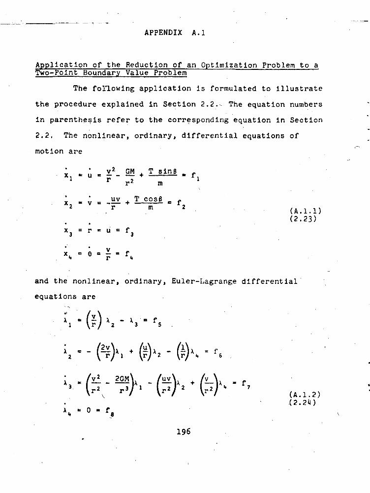
APPENDIX A.I
Application of the Reduction of an Optimization Problem to aTwo-Point Boundary Value Problem ~
The following application is formulated to illustrate
the procedure explained in Section 2.2.- The equation numbers
in parenthesis refer to the corresponding equation in Section
2.2, The nonlinear, ordinary, differential equations of
motion are
i . u = v2. OM + T_sin3 .r r2 m
i . ; „ .Hi + T_cos0 . f2 . r m 2 (A. 1.1)
(2 .23)* •
x3 = r = u * f
and the nonlinear, ordinary, Euler-Lagrange differential
equations are
- V fs .
Xi . i2M\A . /uvV + A \ .* P > ; > v - 2 / 2 v^r. 7(A.1.2)
196
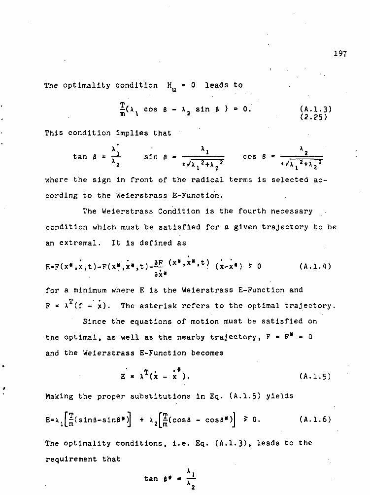
197
The optimality condition H « 0 leads to
-(Xt cos 6 - X, sin 0 ) = 0. (A. 1.3)m 1 2 (2.25)
This condition implies that
X* Xl X» '
tan 8 * r-i- sin 6 = — - _ ••• cos 8 « — _X2 t/A^ + Xj2 '/x^+Xj2
where the sign in front of the radical terms is selected ac-
cording to the Weierstrass E-Function.
The Weierstrass Condition is the fourth necessary
condition which must be satisfied for a given trajectory to be
an extremal. It is defined as•
E-P(x«,i,t)-P(x«,x«,t)-^ (**iX".t) (X,x«) 5 o (A. 1.4)
for a minimum where E is the Weierstrass E-Function and<P .
F * X (f - x). The asterisk refers to the optimal trajectory.
Since the equations of motion must be satisfied on
the optimal, as well as the nearby trajectory, F = F* s 0
and the Weierstrass E-Function becomes
E - XT(x - x ). (A. 1.5)
Making the proper substitutions in Eq. (A. 1.5) yields
E=x,J-(sinS-sinB»)| + X-F-CcosB - cos8*)l ? 0. (A. 1.6)ILm J 2|_m J
The optimality conditions, i.e. Eq. (A. 1.3), leads to the
requirement thatAi
tan e» • ~2

198
which Implies
sin 6 - — — and cos e« - 2 - . (A.1.7)'/x^+Xj2 , *Al
2-»-x22
Eq. (A.1.3) does not indicate which sign should be selected on*
the radical terms. Substituting Eq. (A.1.7) into Eq. (A.1.6)
yields ^
E m Xi +X2 U -1 + cos (B - 8 ' ° and (A.1.8)
for this equation to be satisfied for all admissible
values of e , the negative sign on the radical must be
chosen. Hence, the optimal control program is given by
x. • .'sin e*
i
x2cos 3" «= — '
The specified initial boundary conditions are
u(tQ) - UQ = 0
n - g2 - v(tfl) - .v0 - 02 2 (A.1.9)(2.26)
n, = g, B r(t0) - r0 = 0
where tQ is specified. Hence no initial conditions are obtained
from the transversality conditions because the initial state
and time are specified.
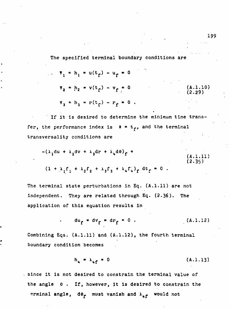
199
The specified terminal boundary conditions are
. . *! c hx « u(tf) - Uf - 0
*2 » h, • v(tr) - v o 0 (A. 1.10)2 "2 f *> (2.29)
*3 * h3 = r(tf) - rf - 0 .
•
If it is desired to determine the minimum time trans-
fer, the performance index is * » t-, and the terminal
transversality conditions are
-(X.du + X,dv + x.dr + X.de). +1 2 3 •» f (A. 1.11)
(2.35)(i + _x jr l + x2f2 + x3f 3 + *k
f^f dtf • o .
The terminal state perturbations in Eq. (A. 1.11) are not
independent. They are related through Eq. (2.36). The
application of this equation results in
duf - dvf - drf « 0 . (A. 1.12)
Combining Eqs. (A. 1.11) and (A. 1.12), the fourth terminal
boundary condition becomes
\ - XHf - 0 (A. 1.13)
since it is not desired to constrain the terminal value of
the angle 0 . If, however, it is desired to constrain the
erminal angle, def must vanish and \kf would not

200
necessarily be zero. In this case, the fourth terminal
boundary condition becomes
ht( «= 0(tf) - ef - 0' . (A.1.11)4
Allowing for the possibility of a variable terminal .
time, Eq. (A.1.11) also yields the fifth and last terminal
condition
•
h5 = (1 + - X l f l + A2f2 + X3f3 .+ fk}t = 0. (A.1.15)
If it is desired to normalize the Lagrange multipliers
as discussed in Section 7.3.1, one multiplier is initially
selected plus or minus.unity and one terminal boundary condi-
tion is ignored. The initial boundary condition
X3 (tQ) «* -1.0 , is used in place of the fifth terminal bound-
ary condition, and the result is
g • u(t ) - u • 01 ° ° h, « u(tp) - U, «= 0 (A.1.16)
g, " v(t ) - v • 02 0 0
g3 - r(t0) - r0 - 0
,2 ° v(tf) - vf « 0
- r(tf) - rf • 0
g, - e(t0) - e0 = ohn
8^ " *,(tft) * 1.0 - 0

201
For the solution of 2n differential equations,
2n+2 boundary conditions must be known. Assuming that the
initial time is zero, 2n+l conditions are needed. These
are the boundary conditions given above.

_._.__ APPENDIX A. 2
Discussion of the Applications
The example class of problems used to apply the
theoretical formulations presented in Chapters 3, ^, and
5 is the minimum time trajectory of a thrusting spacecraft
under the influence of an inverse square gravitational
force field. The specific examples used to obtain the
numerical results discussed in Chapter 6 are:
(1) A constant low thrust Earth-Mars transfer tra-
jectory which leaves the Earth's circular orbit about
the Sun with a velocity equal to that of the Earth.
The control or thrust angle is unbounded and only
the Sun's gravitational influence is considered.
x The spacecraft arrives at an arbitrary heliocentric«
angle in the circular Mars orbit having velocity
conditions that match that of Mars.
\(2) A constant high thrust Earth launch to a 100
kilometer circular orbit leaving the Earth's sur-
face with zero velocity. The control or thrust
angle is unbounded. The Earth's inverse square
gravitational influence is considered. The dissa-
pative terms of the atmospheric drag are also included,
The spacecraft arrives at an arbitrary heliocentric
202

203
angle in the circular orbit. The effects of other
bodies are neglected.
In the optimization reduction problem shown in Appen-
dix A.I it is seen that the initial state Is specified and
hence n » p = 4 . The terminal velocity and radial position
are specified and hence q = 3 • TWO additional terminal
constraints are derived from the transversality conditions.
Assuming that the initial time is specified as zero, five
initial conditions and five terminal conditions are speci-
fied, therefore the problem is solvable.
When the numerical parameters are normalized as dis-
cussed in Section 7.3.1* the initial value of the Lagrange
multiplier associated with the radius is equated to a negative
unity, and hence p = 5 , and the last transversality condi-
tion is ignored. This means that six initial conditions«and
four.terminal conditions are specified, where the initial time
is Included. The problem is still solvable, but the com-
plexion of the applications is changed slightly from that
described in the detailed procedures presented in Chapters
3 and H.
It should be pointed out that the fourth differential
equation of state and the corresponding Euler-Lagrange equa-
tion is not necessary for the analysis made here. These
equations are simply included for the sake of generality,

PO/I
and hence the same computer programs may easily be converted
to solve the class of problems where terminal, state is com-
pletely specified.
The time histories of each variable that correspond
to the optimal solution for the Earth-Mars transfer are il-
lustrated in Figure A.5.1. The optimal control history for
this problem is shown in Figure A.5.2. The time histories
of each variable that correspond to the optimal solution for
the Earth launch are illustrated in Figure A.5.3. The opti-
mal control history for this problem is shown in Figure A. 5 • ** •

205
Uto -w
if*3
0 o , /»"5_o 1.0
J S *•e o
?rt
Nonlinearoptimal
Linearinitial solution
Constantinitial solution
0 20 40 60 80 100 120 140 160 180 20(3
c.v
S i ?
Iin to1=5 , o|| 1-°
'c • £3 ••*
0
3 A.u
•2 20-o '••*'SCJ•- 1 ften l.Uc
*••
2
.
— -
0 4
^*
— ... ••
0 6
^g- ««r^«^
0 80 1C
^essJ
)o i;
-sr "
^S** **
?0 1*
^—
10 16
^^^^^^^»
)0 11
•ffSff*
30 20 0
0 20 40 60 80 100 120 140 160 180 200Time, days
Figure A.2.1 - Optimal trajectory for the Earth-Mars transfer.

206
-1.00 20 40 60 80 100 120 140 160 180 200
Time, days
CM
0 20 40 60 80 100 120 140 160 180 200
Time, days
0 20 40 -60 80 100 120 140 160 180 200Time, days
Figure A.2.1. - Optimal trajectory for Earth-Mars transfer (con't).

330207
o>
CJ>
encre
300
270
240
210
180
150
120
90
60
30
0 20 40 60 80 100 120 140 160 180 200
Mission time, days
Figure A.2,2. - Optimal constant and unbounded thrust program for theEarth-Mars transfer. '

208
800
.082'± .04e>
300
300
300
50 100 150
Time, seconds200 250 300
Figure A.2.3. - ^Optimal trajectory for the atmospheric Earth launch,

209
0 -
-100 I-
-200
-300' 100 150 200 250 300
u
^-100
-20050 100 150 200 250 300
u
-.4
-.8
1.2
1 A50 100 150 200 250 300
Figure A.2.3. - Optimal trajectory for the atmospheric Earth launch(cont),

210
70
60
50
I/IOl
en0)
• 30
JL ^
\
Cre
S 20
10
-10
-2050 100 150
Time, seconds
200 250 300
Figure A.2.4. - Optimal constant and unbounded thrust program forthe atmospheric Earth launch.
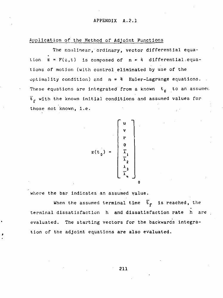
APPENDIX A. 2.1
Application of the Method of Adjoint Functions
The nonlinear, ordinary, vector differential equa-*
tlon z = F(z,t) is composed of n = ^ differential equa-
tions of motion (with control eliminated by use of the
optimal ity condition) and n = ^ Euler-Lagrange equations.
These equations are integrated from a known tfl to an assumec
tff with the known initial conditions and assumed values for
those not known, i.e. .
u
V
rG
*(tfl> =
where the bar indicates an assumed value.
When the assumed terminal time tf is reached, the•
terminal dissatisfaction h and dissatisfaction rate h are
evaluated. The starting vectors for the backwards integra-
tion of the adjoint equations are also evaluated.
211

212
These adjoint equations, A » - are
./Zi.2Sfi\. . /HI\, +/v_3 Vr2 rV ' VrV J ^2
A «= 0
r
TX
n ( X 12 + X 2
2 ) 3 / 2
r T x , x 2
m ( X l2 , X 2
2 ) V 2 _
A -1
A xT
TX X1 2
_ m ( X l 2 + X 22 ) 3 / 2 _
" TX 2
i
m(x , 2 +x 2 )• i A — '
(-) vC-f -
and are integrated backwards from tf to t forming the\
coefficients from the variables stored during the forward

213
integration. The 2n+l-p = 4; starting vectors for this back-!
ward integration are
w •
10000000
A 2 ( t f ) =
0100000
_ . o _
A 3 ( t f ) =
00100000
w •
00000001
When the initial time tfl is reached, 2n+l-p
algebraic equations are solved for the linear estimates for
the corrections that must be applied to the assumed initial
conditions (^i0» *2o* \o^ anc^ the assume(* terminal time
(t_). These algebraic equations are
-. r- ~i ~1 r~^ ' "~ du9
9
8i
82
u
953 963 983 rf
dv
dr
where the elements of the e matrix are evaluated at t Q.
These corrections are applied to the initially assumed values
of T., T , IT and tff and a new nominal trajectory is
Integrated using z • F(z,t) .
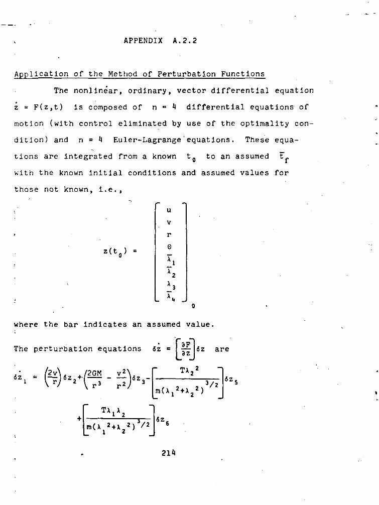
APPENDIX A.2.2
Application of the Method of Perturbation Functions
The nonlinear, ordinary, vector differential equation
z = F(z,t) is composed of n = 4 differential equations of
motion (with control eliminated by use of the optimality con-
dition) and n = 4 Euler-Lagrange'equations. These equa-
tions are integrated from a known tfl to an assumed tf
with the known initial conditions and assumed values for
those not known, i.e.,
z ( t 0 ) =
u
V
r
0
T2
where the bar indicates an assumed value
The perturbation equations 6z = — 6z are
6z • $)•*>+&* -m(\l
Tx

215
3 <°:Tx 21 A i
3/2
3/2
;3 = «Zl
6z, = F - ••) •6Z5 - V-
' 2X
,F 6Z6 - 6Z7
fe^-
(»K - ffl 6z.
6Z_ • -I v-+PLr
x /6GM
r ^ V ^
/v2
fc-
•f 2uvX, - 2vX, 6 Z .
2QMrV 5 Vr2/
6ze - — Uz, + /— Uz
0 ,
and are integrated forwards from tQ to tf forming the
coefficients from the variables calculated by the integration
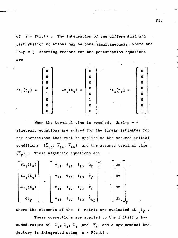
216
of z = F(z,t) . The integration of the differential andv
perturbation equations may be done simultaneously, where the
2n-p » 3 starting vectors for the perturbation equations
are
0000000
When the terminal time is reached, 2n+l-p » 4
algebraic equations are solved for the linear estimates for
the corrections that must be applied to the assumed Initial
0
0
0
010
0
0
6 z 2 ( t 0 ) =
ro0
0
0010
0
conditions (*"10iand the assumed terminal time
(tf-) . These algebraic equations are
12 U-1V
du
dv
dr
*21 *22 *23 Vf
A A A
31 32 33
83
where the elements of the * matrix are evaluated at tf .
These corrections are applied to the initially as-
sumed values of T , T2, T^ and Ff and a new nominal tra-•
Jectory is Integrated using z * P(z , t ) .

APPENDIX A.2.3
Application of the Modified Quasillnearlzatlon Method
The nonhompgeneous linear, ordinary vector differen-
tial z = Az + B is composed of n » 4 linearized differ-
ential equations of motion (with the control eliminated by
use of the optlmality condition) and n « *l linearized
Euler-Lagrange equations. These equations are
; « u „ /W\'Wi n*1 \r/n
+ /2GM _ vi
n
n-n
'n-n
-©„ ""*' - ©n V"+' + (Dn
TX,ia2 Z . 3Z
n *n
217

S18
m Q »
n+i 8n
A2 \ / 2XAze « x - (-i) u - [ U v
«n+i 2n+i \ r/n n+l V r /n n+1
n(B»)nn
r *


<?,)„
<Be>n '
220
these nonhomogeneous linear equations are Integrated
from tQ to/ tf with the starting vector
uV
rer.
where the bar Indicates an assumed value. This determines
the variables for the n+1 Iteration by using the vari-
ables resulting from the n Iteration to form the re-
quired coefficients.
The homogeneous linear equations (same as above ex-
cept without the (BA)n , 1 « 1, 2n terms) y • Ay, are

c <• 1
integrated from tQ u c_ in.the same manner as the non-
homogeneous equations but with the 2n-p=3 starting vectors
, - • : ' " • • ; ! - • • 1 0ij
0
1 '
0
0
0
y 2 ( t o ) n-n "
\
u
0
0
10
0
y 3 ( t 0 ) +1: -
f
-.0
o':0i
rCM
When the terminal time is reached, 2n+l-p = 1
algebraic equations are solved for the corrections that must
be applied to the assumed initial conditions (*\o> ^20* "*MQ
and the assumed terminal time (tf) . These algebraic equa-
tions are
0
— - •
yi 1 yi2 yi3 Uf•
v y v v«^21 Jr22 ^23 f
a
V - V o o V o o I *3i 32 JJj f
•
81 82 83 Uf^
-1 du
dv
dr
d\M-I f
where the elements of the matrix are- evaluated at t_.
These corrections -are applied to the initially as-
sumed values of T , T , and tf and a new nominal tra-
jectory is integrated using z » Az+B . where the A and B
matrices are formed from the previous nominal.

APPENDIX A.2.H
Application of the Method of Steepest Descent
The nonlinear, ordinary, vector differential equation
x« f(x,u,t)( is composed of n « *l differential equations
of motion. These equations are integrated forward with the
initial conditions
uvre
and the initial estimate of the control program u(t) .
The performance index to be minimized is
and the terminal constraints are
u(tf) - uf » 0
v(tf) - vf - 0
r(tf) - rf « 0
The condition that is used to atop the integration is
fl » e(t 0 .
222

223
The equations adjoint to the differential equationsm ;
of motion, x • -f X , are
- x
\ • ° >and the starting conditions for the backward integration are,
[0 0 0 0]
10
0
0
10
0
0
1
0
0
0
<s<v • [4 [0 1] .
The time rates of change of the performance index,
terminal constraints and stopping condition are

sta
for
are
.'••0

APPENDIX A.2.5
Application of the Modified Method of Steepest Descent
The nonlinear, ordinary, vector differential equation• .
x » f(x,u,t) is composed of n • 4 differential equations
of motion. These equations are integrated forward with the
initial conditions
x(t0) -
and the initial estimate of the control program u(t)
The penalty function to be minimized is
P - W0tf2+W1[u(tf)-uf]
2+W2[v(tf)-vf]2*W3[r(tf)-rf]
2
and the stopping condition is 7
n « e(tf) - ef • o .
The equations adjoint to the differential equationsTof motion, X « -f X , are
225

126
; ._/2°«_viV _/uv1 ^r' r'/ ' ^r
0 -
The starting conditions for the backward integration
are
m - Bwhere
2WiCu(tf) -
- v,]
f3[r(tf) - rf]
. f + Xpo f + XpQ f + 2W t•l . 1 Pn2 2 p"3 3 0 1
The new control program is given by
sin 8 - AB_ cos 8)

APPENDIX A.3
Numerical Constants
Earth-Mars Transfer.
Astronomical Unit, AU
Orbital Radius of Earth, r
Orbital Radius of Mars, rmGravitational Constant of Sun, GMs
Initial Spacecraft Mass, m
Thrust, Tt
Mass Rate, m
.11*959870 X 1012 meters
.10000000 X IO1 AU
.15236790 X 101 AU
.1327150*1 x io21
metersVsecond*
.67978852 X IO3 kilograms
.1*0312370 X 101 newtons
.10123858 X 10~*kilograms/second
Earth Launch
.63781700 X IO7 metersRadius of Earth, Rfi
Gravitational Constant of Earth, GMe .39860610 X IO15
meters'/second2
Initial Spacecraft Mass, m
Thrust, T
Mass Rate, m
.15000000 X 10" kilograms
.27000000 X IO5 newtons
.1*5000000 X IO1
kilograms/second
The terms that must be added to the differential
equations f1 and f2 to Include atmospheric resistance
are:
227

228
fl i ^ m
f, - f, -
r-Re .. ;where p = p e E (ma iensity)
CD; « Q..3, 0 < M < .6950 (dr. coefficient)
'• •' . - ' •-•-.' " K- K, ' . • .-:•'••'••Cn « K. + — =-, M > .6950
•' - }' ^M2 M3
M * — (mach number)a
a e D - B(r - Re) (speed of sound)
and where
:. >
p * 0.52 kilograms/meter3
E « 7600.0 meters
Kj « 0.1368.
: K2 » 1.6218
K-3 * 1.072ft
- , • . . - • . •* - : -, • • '
D • 3 f t O . O meters/second
B • 0.00071 Vseconds
A • ft.O meters2

APPENDIX A.H
Normalization Scheme
Earth-Mars Transfer
Unit of Lensth (1 AU)
Unit of Mass (m ): " . ' . ' . °
Unit of Velocity v «=V—~e ? r.
Unit of Force
Unit of Time
.14959870 X 1012 meters
.67978852 X 103 kilograms
.29784901 X.105
meters/second
.40312370 X 101 newtons
.50226355 X 107 seconds
.58132355 X 102 days
The normalized values of the. parameters of Interest are :
, .Gravitational Constant of Sun, GM - = 1.0g
Initial Spacecraft Mass * 1.0
Initial Spacecraft Velocity -1.0
.Initial Spacecraft Radius » 1.0
Terminal Spacecraft Velocity • 0.81012728
.Terminal Spacecraft Radius • 1.5236790
Thrust « .11012969
Mass Rate - 0.07^800391
Earth Launch - No normalization scheme.
229

BIBLIOGRAPHY
1. Lawden, D. P., "Optimal Programming of Rocket ThrustDirection," presented at the Fifth I.A.P. Congressat Innsbruck, August 6, 195''.
2. Breakwell, J. V., "The Optimization of Trajectories,"North American Aviation, Inc., Report AL-2706,August 1957.
3. Kelley, H. J., "Gradient Theory of Optimal Flight Paths,"ARS Journal (now AIAA Journal), p. 9^7, October I960.
1*. Mac Kay, J. S. , Rossa, L. G. , and Zimmerman, A. V.,"Optimum Low-Acceleration Trajectories for Earth-MarsTransfer," Proceedings of the IAS Symposium on VehicleSystem Optimization, Garden City, N.Y.. Nov. 28-29.1961.
5. Melbourne, W. G., Sauer, C. G., Jr., and Richardson,D. E'. , "Interplanetary Trajectory Optimization withPower-Limited Propulsion Systems," Proceedings ofthe IAS. Symposium on Vehicle System Optimization.Garden City, N.Y., Nov. 28-29, 1961.
6. Scharmack, D. K., "The Equivalent Minimization Problemand the Newton-Raphson Optimization Method," Proceed-ings from Optimum System Synthesis Conference, Wright*-2jf, SPatterson Air Force Base, September 1962, p.119-158.
7. 'Jurovics, S. A. and Mclntyre, J. E., "The Adjoint Methodand its Application to Trajectory Optimization," ARSJournal. p. 135**, September 1962.
8. Goodman, T. R. and Lance, G. N., "The Numerical Integra-tion of Two-Point Boundary Value Problems," MathTables and Other Aids to Computation, Vol. 10, p.82, 1956.
9. Breakwell, J. V., Speyer, J. L., and Bryson, A. E.,"Optimization and Control of Nonlinear Systems Usingthe Second Variation," Journal of the Society ofIndustrial and Applied Mathematics Control, Ser. A,Vol. 1, No. 2, p. 193-223, 1 9 6 3 . ~
10. Breakwell, J. V., "The Optimization of Trajectories,"Journal of the Society of Industrial and AppliedMathematics, Vol. 7, No. 2. p. 215-247, June 1959.
230

231
11. Kelley, H. J., Kopp, R. E., and Moyer, H. G., "A Tra-jectory Optimization Technique Based Upon the Theoryof • the = Second Variation," presented at the AIAA
: Astrodynamics -Conference, Yale University, NewHaven, Conn., August 19-21, 1963.
12. Jazwinski, A*. H., "Optimal Trajectories and Linear Con-trol of Nonlinear Systems," AIAA Journal, Vol. 2,No. 8, p. 1371, August 1964.
13. McGill, R. and Kenneth, P., "Solution of VariationalProblems, by Means of a Generalized Newton-RaphsonOperator," AIAA Journal, Vol. 2, No. 10, p. 1761,October 196T.
1^. Kalaba, R. , "Nonlinear Differential Equations, the Maxi-mum Operation, and Monotone Convergence," Journal ofMathemat ic s and Mechanic s , Vol. 8, No. 4, p. 519-574,1959.
15. McGill, R. and Kenneth, P., "A Convergence Theorem onthe Iterative Solution of Nonlinear Two-Point Bound-ary Value Systems,"- presented at the XIV Inter-national Astronautical Congress, Paris, September 25,
•'.•1963..
16. Long, R. S., "Newton-Raphson Operator; Problems withUndetermined End Points," AIAA Journal, Vol. 3,
: No. 7, p. 1352, July 1965-
17. Bryson, A. E. , Denham, W. P., Carroll, F. J., and Mikami,K., "Determination of Lift or Drag Programs to Mini-mize Re-Entry Heating," Journal of the AerospaceSciences, p. 420, April 1962.
18. Bryson, A. E, and Denham, W. P., "A Steepest-AscentMethod for Solving Optimal Programming Problems,"Journal of Applied Mechanics, p. 247, June 1962.
19. Kelley, H. J., Kopp, R. E. , and Moyer, H. G., "Succes-sive Approximation Techniques for Trajectory Optimi-zation," Proceedings of the IAS Symposium on VehicleSystem Optimization. Garden City, N.Y.. Nov. 28-29.
20. Pfeiffer, C. G. , "Theory and Application of the CriticalDirection Method of Trajectory Optimization," Pro-ceedings of the IAS Symposium on Vehicle SystemOptimization, Garden City, N.Y., Nov. 2B-29, 1961 .

232
21. Wagner, W. E. , . Jazwinski, A. H., "Three-Dimensional Re-Entry Optimization with Inequality Constraints," ForPresentations, Astrodynamics Conference of the AIAA,Yale University, New Haven, Conn., August 19-21, 1963.
22. Rosenbaum, R^ , "Convergence Technique for the Steepest-Descent Method of Trajectory Optimization," AIAAJournal, Vol. 1, No. 7, p. 1701, July 1963.
23. Stancil, R. T. , "A New Approach to Steepest-Ascent Tra-jectory Optimization," AIAA Journal. Vol. 2, No. 8,p. 1365, August 1964.
2*4. McReynolds, S. R. and Bryson, A. E., Jr., "A SuccessiveSweep Method for Solving Optimal Programming Prob-lems," Tech. Report No. 463, Cruft Laboratory,Harvard University, Cambridge, Mass., March 1965.
25. Kopp, R. E. and McGill, R. , "Several Trajectory Optimi-zation Techniques Part I," Computing Methods in Opti-mization Problems, Academic Press, 1961. •
26. Moyer, Gardner H. and Pinkham, Gordon, "Several Trajec-tory Optimization Techniques Part II," ComputingMethods in Optimization Problems, Academic Press,~
27. Gelfand, I. M. and Fomin, S. V., Calculus of Varia-tions, Prentice Hall, 1963.
- -~s t
28. Melbourne, W. G., "Three-Dimensional Optimum ThrustTrajectories for Power Limited Propulsion Systems,"ARS Journal, December 1961, p. 1723.
29. Merriam, C. W. , "An Algorithm for the Iterative Solu-tion of a Class of Two-Point Boundary Value Problems,Journal of the Society of Industrial and AppliedMathematics Control, Ser. A., Vol. 2, No. 1,pp. 1-10, 1961.
30. Sylvester, R. J. and Meyer, F. , "Two Point BoundaryProblems by Quasilinearization," Journal of theSociety of Industrial and Applied Mathematics, Vol.13, No. 2, pp. 586-602, June 1965.
NASA MSC Cornl.. Houston,.Texas