Introduction to MagnetoHydroDynamics (MHD)

Antoine Cerfon, Courant Institute, New York UniversityEmail: cerfon@cims.nyu.edu

SULI Introductory Course in Plasma Physics, June 8, 2015

PART I: DESCRIBING A FUSION PLASMA

METHOD I: SELF-CONSISTENT PARTICLE PUSHINGI An intuitive idea is to solve for the motion of all the particles

iteratively, combining Newton’s law with Maxwell equationsI At each time step i, solve

md2x(i)

kdt

= qk

(E(xk)

(i−1) +dx(i)

kdt× B(i−1)(xk)

)k = 1, . . . ,N

(∂E∂t

)i

= c2∇× B(i−1) − µ0c2N∑

k=1

qkdxi

kdtδ(x− xi

k)(∂B∂t

)i

= −∇× Ei

I Fast solvers exist for the electromagnetic fields, some relying ona subsidiary mesh, some not needing a mesh

I Even with fast solvers, problem still not tractable even with themost powerful computers when N ∼ 1020 − 1022 as in magneticfusion grade plasmas

METHOD II: COARSE-GRAIN AVERAGE IN PHASE

SPACE

(From G. Lapenta’s: https://perswww.kuleuven.be/ u0052182/weather/pic.pdf )I For hot and diffuse systems with a large number of particles,

following every single particle is a waste of time and resourcesI Replace the discrete particles with smooth distribution function

f (x,v, t) defined so that

f (x,v, t)dxdv

is the expected number of particles in the infinitesimalsix-dimensional phase-space volume dxdv.

DISTRIBUTION FUNCTION AND VLASOV EQUATIONI Macroscopic (fluid) quantities are velocity moments of f

n(x, t) =

∫∫∫f (x,v, t)dv Density

nV(x, t) =

∫∫∫vf (x,v, t)dv Mean flow

P(x, t) = m∫∫∫

(v−V) (v−V) fdv Pressure tensor

I Conservation of f along the phase-space trajectories of theparticles determines the time evolution of f :

dfdt

=∂f∂t

+dxdt· ∇f +

dvdt· ∇vf = 0

dxdt

= vdvdt

=qm

(E + v× B)

⇒ ∂f∂t

+ v · ∇f +qm

(E + v× B) · ∇vf = 0

This is the Vlasov equation

THE BOLTZMANN EQUATION

I In fusion plasmas, we separate, leading to the Boltzmannequation:

∂f∂t

+ v · ∇f +qm

(E + v× B) · ∇vf =

(∂f∂t

)c

This equation to be combined with Maxwell’s equations:

∇× E = −∂B∂t

∇× B = µ0J +1c2∂E∂t

I Nonlinear, integro-differential, 6-dimensional PDEI Describes phenomena on widely varying length (10−5 – 103 m)

and time (10−12 – 102 s) scalesI Still not a piece of cake, and never solved as such for fusion

plasmas

MOMENT APPROACH

∂f∂t

+ v · ∇f +qm

(E + v× B) · ∇vf =

(∂f∂t

)c

I Taking the integrals∫∫∫

dv,∫∫∫

mvdv and∫∫∫

mv2/2dv of thisequation, we obtain the exact fluid equations:

∂ns

∂t+∇ · (nsVs) = 0 Continuity

mn(∂Vs

∂t+ Vs · ∇Vs

)= qsns (E + Vs × B)−∇ · Ps + Rs Momentum

ddt

(32

ps

)+

52

ps∇ ·Vs + πs : ∇Vs +∇ · qs = 0 (Energy)

with Ps = psI + πs.I Closure problem: for each moment, we introduce a new

unknown ⇒ End up with too many unknownsI Need to make approximations to close the moment hierarchy

KINETIC MODELS VS FLUID MODELS

I For some fusion applications/plasma regimes (heating andcurrent drive, transport), kinetic treatment cannot be avoided

I Simplify and reduce dimensionality of the Vlasov equation withapproximations:

I Strong magnetization : Gyrokinetic equationI Small gyroradius compared to relevant length scales : Drift

kinetic equationI Vanishing gyroradius : Kinetic MHD

I In contrast, fluid models are based on approximate expressionsfor higher order moments (off-diagonal entries in pressuretensor, heat flux) in terms of lower order quantities(density,velocity, diagonal entries in pressure tensor)

I We will now focus on the relevant regime and theapproximations made to derive a widely used fluid model: theideal MHD model

PART II: THE IDEAL MHD MODEL

LAWSON CRITERION AND MHD

Condition for ignition: pτE ≥ 8 bar.s Tmin ∼ 15keV

I The maximum p is limited by the stability propertiesJob of MHD

I The maximum τE is determined by the confinementpropertiesJob of kinetic models

PHILOSOPHY

I The purpose of ideal MHD is to study the macroscopic behaviorof the plasma

I Use ideal MHD to design machines that avoid large scaleinstabilities

I Regime of interestI Typical length scale: the minor radius of the device a ∼ 1m

Wave number k of waves and instabilitities considered: k ∼ 1/a

I Typical velocities: Ion thermal velocity speed vT ∼ 500km/s

I Typical time scale: τMHD ∼ a/vT ∼ 2µsFrequency ωMHD of associated waves/instabilities ωMHD ∼ 500kHz

EXAMPLE: VERTICAL INSTABILITY

Figure from F. Hofmann et al., Nuclear Fusion 37 681 (1997)

IDEAL MHD - MAXWELL’S EQUATIONS

I a� λD, the distance over which charge separation can take placein a plasma⇒ On the MHD length scale, the plasma is neutral : ni = ne

I ωMHD/k� c and vTi � vTe � c so we can neglect thedisplacement current in Maxwell’s equations:

ni = ne

∇ · B = 0

∇× E = −∂B∂t

∇× B = µ0J

IDEAL MHD - MOMENTUM EQUATION

I a� λD and a� rLe (electron Larmor radius)I ωMHD � ωpe, ωMHD � ωce

I The ideal MHD model assumes that on the time and lengthscales of interest, the electrons have an infinitely fast responsetime to changes in the plasma

I Mathematically, this can be done by taking the limit me → 0I Adding the ion and electron momentum equation, we then get

ρdVdt− J× B +∇p = −∇ · (πi + πe)

where ρ = min and V is the ion fluid velocityI If the condition vTiτii/a� 1 is satisfied in the plasma

ρdVdt

= J× B−∇p (Ideal MHD momentum equation)

IDEAL MHD - ELECTRONS

I In the limit me → 0, the electron momentum equation can bewritten as

E + V× B =1en

(J× B−∇pe −∇ · πe + Re)

I This is called the generalized Ohm’s lawI Different MHD models (resitive MHD, Hall MHD) keep

different terms in this equationI If rLi/a� 1, vTiτii/a� 1, and (me/mi)

1/2(rLi/a)2(a/vTiτii)� 1, themomentum equation becomes the ideal Ohm’s law

E + V× B = 0

I The ideal MHD plasma behaves like a perfectly conducting fluid

ENERGY EQUATION

I Define the total plasma pressure p = pi + pe

I Add electron and ion energy equations

I Under the conditions rLi/a� 1 and vTiτii/a� 1, this simplifies as

ddt

(pρ5/3

)= 0

I Equation reminiscent of pVγ = Cst: the ideal MHD plasmabehaves like a monoatomic ideal gas undergoing a reversibleadiabatic process

IDEAL MHD - SUMMARY

∂ρ

∂t+∇ · (ρV) = 0

ρdVdt

= J× B−∇p

ddt

(pρ5/3

)= 0

E + V× B = 0

∇× E = −∂B∂t

∇× B = µ0J∇ · B = 0

Valid under the conditions(mi

me

)1/2 (viτii

a

)� 1

rLi

a� 1

(rLi

a

)2(

me

mi

)1/2 avTiτii

� 1

VALIDITY OF THE IDEAL MHD MODEL (I)I Are the conditions for the validity of ideal MHD(

mi

me

)1/2 (viτii

a

)� 1

rLi

a� 1

(rLi

a

)2(

me

mi

)1/2 avTiτii

� 1

mutually compatible?I Define x = (mi/me)

1/2(vTiτii/a), y = rLi/a.

x� 1 (High collisionality) y� 1 (Small ion Larmor radius)

y2/x� 1 (Small resistivity)

There exists a regime for whichideal MHD is justified (Figurefrom Ideal MHD by J.P. Freidberg,CUP, 2014)

Is that the regime of magneticconfinement fusion?

VALIDITY OF THE IDEAL MHD MODEL (II)

I Express three conditions in terms of n, T, a and β, with β theratio of plasma pressure and magnetic pressure

I For β = 5% and a = 1m (realistic fusion parameters), we find

The regime of validity of idealMHD does NOT coincide with thefusion plasma regime (Figurefrom Ideal MHD by J.P. Freidberg,CUP, 2014)

The collisionality of fusionplasmas is too low for the idealMHD model to be valid.

Is that a problem?

VALIDITY OF THE IDEAL MHD MODEL (III)

I It turns out that ideal MHD often does a very good job atpredicting stability limits for macroscopic instabilities

I This is not due to luck but to subtle physical reasons

I One can show that collisionless kinetic models for macroscopicinstabilities are more optimistic than ideal MHD

I This is because ideal MHD is accurate for dynamicsperpendicular to the fields lines

I Designs based on ideal MHD calculations are conservativedesigns

FROZEN IN LAW (I)I E + V× B = 0: in the frame moving with the plasma, the electric

field is zeroI The plasma behaves like a perfect conductorI The magnetic field lines are “frozen” into the plasma motion

⇒

FROZEN IN LAW (II): PROOFI ∂B/∂t = ∇× E , E + V× B = 0⇒ ∂B/∂t = ∇× (V× B)I Calculate the change in the flux Φ =

∫∫S(t) B · ndS across a

moving surface with velocity u⊥Image from Principles ofMagnetohydrodynamics WithApplications to Laboratory andAstrophysical Plasmas by J.P.Goedbloed and S. Poedts,Cambridge University Press(2004)

dΦ

dt=

∫∫S(t)

∂B∂t· ndS−

∮∂S(t)

u⊥ × B · dl

=

∫∫∇× (V× B) · ndS−

∮∂S(t)

u⊥ × B · dl

=

∮∂S(t)

(V− u⊥) · dl

= 0 if u⊥ = V

i.e. the plasma is tied to the field lines

MAGNETIC RECONNECTIONImage from Principles ofMagnetohydrodynamics WithApplications to Laboratory andAstrophysical Plasmas by J.P.Goedbloed and S. Poedts,Cambridge University Press(2004)

I Magnetic reconnection: a key phenomenon in astrophysical,space, and fusion plasmas

I Cannot happen according to ideal MHD

I Need to add additional terms in Ohm’s law to allowreconnection: resistivity, off-diagonal pressure tensor terms,electron inertia, . . .

I Associated instabilities take place on longer time scales thanτMHD

PART III: MHD EQUILIBRIUM

EQUILIBRIUM STATE

I By equilibrium, we mean steady-state: ∂/∂t = 0I Often, for simplicity and/or physical reasons, we focus on static

equilibria: V = 0

∇ · B = 0∇× B = µ0JJ× B = ∇p

A more condensed form is

∇ · B = 0 (∇× B)× B = µ0∇p

Note that the density profile does not appear

1D EQUILIBRIA (I)

θ-pinchZ-pinch

Combine the two to get....

(Figure from Ideal MHD by J.P. Freidberg, CUP, 2014)

1D EQUILIBRIA (II)

Screw pinch

(Figure from Ideal MHD by J.P.Freidberg, CUP, 2014)

I Equilibrium quantities only depend on rI Plug into∇ · B = 0 , (∇× B)× B = µ0∇p to find:

ddr

(p +

B2θ + B2

z2µ0

)+

B2θ

µ0r= 0

Balance between plasma pressure, magnetic pressure, andmagnetic tension

I Two free functions define equilibrium: e.g. Bz and p, or Bθ and Bz

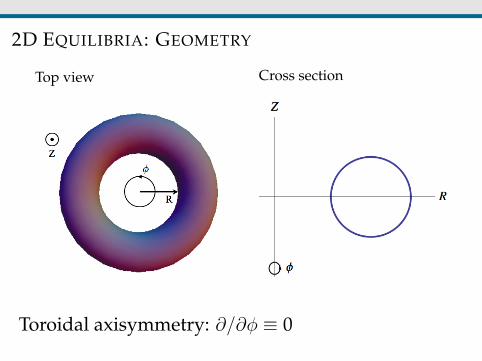
2D EQUILIBRIA: GEOMETRY

Top view Cross section

Toroidal axisymmetry: ∂/∂φ ≡ 0

TOROIDALLY AXISYMMETRIC EQUILIBRIAStep 1:

B = Bφ(R,Z)eφ+Bp(R,Z) and ∇ · B = 0 ⇒ ∇ · Bp = 0

⇒ B = Bφeφ +1R∇Ψ× eφ

Ψ = RAφ, with A vector potential: ∇×A = B.

Step 2:

∇× B = µ0J⇒

µ0Jφ = − 1

R

[R ∂∂R

(1R∂Ψ∂R

)+ ∂2Ψ

∂Z2

]= − 1

R∆∗Ψ

µ0Jp = 1R∇(RBφ × eφ)

Step 3:

J× B = ∇p

·B ⇒ ∇Ψ×∇p = 0 ⇒ p = p(Ψ)

·J = 0 ⇒ ∇(RBφ)×∇Ψ = 0 ⇒ RBφ = F(Ψ)

I The regions of constant pressure are nested toroidal surfaces

I Magnetic fields and currents lie on these nested surfaces

GRAD-SHAFRANOV EQUATION

Last step: [J×B = ∇p] ·∇Ψ gives the Grad-Shafranov equation (GSE):

R∂

∂R

(1R∂Ψ

∂R

)+∂2Ψ

∂Z2 = −µ0R2 dpdΨ− F

dFdΨ

I Second-order, nonlinear, elliptic PDE. Derived independently byH. Grad1 and V.D. Shafranov2.

I The free functions p and F determine the nature of theequilibrium

I In general, the GSE has to be solved numerically

1Proceedings of the Second United Nations Conference on the Peaceful Uses of AtomicEnergy, Vol. 31, p.190

2Sov. Phys. JETP 6, 545 (1958)

EXAMPLES (I)

R/R0

Z/R0

−1.5 −1 −0.5 0 0.5 1 1.5

−0.6

−0.4

−0.2

0

0.2

0.4

0.6

Grad-Shafranov equilibrium for JET tokamak

EXAMPLES (II)

X

Y

−1 0 1

−5

0

5

Grad-Shafranov equilibrium for Field Reversed Configuration

NUMERICAL SOLUTION TO THE GRAD-SHAFRANOV

EQUATION

I Magnetic equilibrium serves as input to stability, wave andtransport codes⇒ important to develop fast and accurate solvers

I Many, many solvers available, from very simple to veryadvanced (FD, FEM, Integral equations, inverse solvers, . . . )

I Free boundary equilibria more challenging than fixed boundaryequilibria

I Equilibria with purely toroidal flow are determined by a closevariant of the Grad-Shafranov equation⇒manyGrad-Shafranov codes can compute such equilibria

Equilibria with both toroidal and poloidal flow can be muchmore challenging; only a handful of codes available

3D EQUILIBRIA (I)

∂/∂φ 6= 0

3D EQUILIBRIA (II)

I Equilibrium equations∇ · B = 0 , (∇× B)× B = µ0∇p still holdI Existence of nested toroidal surfaces not guaranteed anymore

Tokamak

R/R0

Z/R

0

−1.5 −1 −0.5 0 0.5 1 1.5

−0.6

−0.4

−0.2

0

0.2

0.4

0.6

Stellarator (3D)

I Computing 3D equilibria fast and accurately still a challengeI Several existing codes, based on different

assumptions/approximations and used to design and studystellarators: VMEC, PIES, SPEC, HINT, NSTAB

PART IV: MHD STABILITY

WHAT DO WE MEAN BY MHD STABILITY?

I That the plasma is initially in equilibrium does not mean it isgoing to remain there

I The plasma is constantly subject to perturbations, small andlarge

I The purpose of stability studies is to find out how the plasmawill react to these perturbations

I Will it try to return to the initial steady-state?I Will it find a new acceptable steady-state?I Will it collapse?

A MECHANICAL ANALOG

Figure from J.P. Freidberg, Ideal MHD, Cambridge University Press(2014)

SOLVING FULL NONLINEAR MHD EQUATIONS

I Here is an idea to study stability of a magnetically confinedplasma:

I Choose a satisfying plasma equilibriumI Perturb itI Solve the full MHD equations with a computerI Analyze results

I Such an approach provides knowledge of the entire plasmadynamics

I There exist several numerical codes that can do that, for variousMHD models (not only ideal): M3D, M3D-C1, NIMROD

I Computationally intensive

I Get more information than one needs?

Figure from R. Paccagnella et al., Nuclear Fusion 49 035003 (2009)

LINEAR STABILITY (I)I Ideal MHD dynamics can be so fast and detrimental that one

may often require linear stability for the equilibrium

I This can simplify the mathematical analysis tremendouslyI Start with an MHD equilibrium:∇ · B0 = 0 , (∇× B0)× B0 = µ0∇p0

I Take full ideal MHD equations, and write Q = Q0(r) + Q1(r, t)for each physical quantity, where Q1 is considered very smallcompared to Q0

I Drop all the terms that are quadratic or higher orders in thequantities Q1 (linearization)

LINEAR STABILITY (II)

∂ρ1

∂t+∇ · (ρ0v1) = 0

ρ0∂v1

∂t= J1 × B0 + J0 × B1 −∇p1

∂p1

∂t+ v1 · ∇p + γp∇ · v1 = 0

∂B1

∂t= ∇× (v1 × B0)

∇ · B1 = 0µ0J1 = ∇× B1

I By design, the system is now linear in the unknown quantitiesρ1, v1, J1, B1, p1

I Much easier to solve in a computerI There’s a trick that makes life even easier

LINEAR STABILITY (III)I Introduce the plasma displacement vector ξ defined such that

v1 =∂ξ

∂tv1(r, 0) =

∂ξ

∂t(r, 0) ξ(r, 0) = 0

I Linearized ideal MHD equations reduce to

ρ∂2ξ

∂t2 = F (ξ) with

F (ξ) =1µ0{∇ × [∇× (ξ × B0)]} × B0 + (∇× B0)× [∇× (ξ × B0)]

+∇ (ξ · ∇p0 + γp0∇ · ξ)

I F is called the ideal MHD linear force operatorI The problem of linear stability is reduced to an initial value

problem with three linear equations and three unknowns: thecomponents of ξ

LINEAR STABILITY (IV): NORMAL MODE ANALYSISI Even the IVP in the previous slide may give more information

than we needI Sometimes, we just want to know if the equilibrium is stable or

notI A normal mode analysis provides the desired framework for thisI Write ξ(r, t) = ξ (r) e−iωt.ωI > 0 corresponds to exponential growth.

I The linearized momentum equation takes the form

−ρω2ξ = F(ξ)

I ω2 is an an eigenvalue of the linear operator −F(ξ)/ρI It can be showed (some lines of algebra...) that F is a self-adjoint

operatorI In ideal MHD, ω2 is a purely real quantityI ω2 ≥ 0 means the mode is stable; ω2 ≤ 0 means the mode is

unstable

EIGENVALUES IN IDEAL MHD

Figure from Principles of Magnetohydrodynamics With Applications toLaboratory and Astrophysical Plasmas by J.P. Goedbloed and S. Poedts,Cambridge University Press (2004)

ILLUSTRATION: WAVES IN IDEAL MHD (I)

I Consider the stability of an infinite, homogeneous plasma:

B = B0−→ez

J =−→0

p = p0

ρ = ρ0

v = 0

I Given geometry, expand ξ(r) as

ξ(r) = ξeik·r

I Dynamics is anisotropic because of the magnetic field: k⊥ + k‖ez

I Without loss of generality,−→k = k⊥

−→ey + k‖−→ez

ILLUSTRATION: WAVES IN IDEAL MHD (II)I −ρω2ξ = F(ξ) can be written as

ω2ρ0ξ =B2

0µ0

{k×

[k×

(ξ × ez

)]}× ez + γp0kk · ξ

I Writing the expression for each component, we get the system ω2 − k2‖v

2A 0 0

0 ω2 − k2v2A − k2

⊥v2S −k‖k⊥v2

S0 −k⊥k‖v2

S ω2 − k2‖v

2S

ξx

ξy

ξz

=

000

I Two key velocities appear:

vA =

√B2

0µ0ρ0

vS =

√γ

p0

ρ0

vA is called the Alfven velocity, in honor of Hannes Alfven, theSwedish scientist who first described MHD waves, and vs is theadiabatic sound speed

ILLUSTRATION: WAVES IN IDEAL MHD (III)

ω2 − k2‖v

2A 0 0

0 ω2 − k2v2A − k2

⊥v2S −k‖k⊥v2

S0 −k⊥k‖v2

S ω2 − k2‖v

2S

ξx

ξy

ξz

=

000

I For nontrivial solutions, determinant of the matrix should be 0I This leads to the following three possibilities for ω2:

ω2 = k2‖v

2A , ω

2 =k2

2(v2

A + v2S)1±

√√√√1− 4k2‖

k2

v2Av2

S(v2

S + v2A

)2

I One can see that ω2 ≥ 0I The infinite homogeneous magnetized plasma is always MHD

stableI Some of the modes above become unstable in magnetic fusion

configurations, because of gradients and field line curvature

SHEAR ALFVEN WAVE

I Branch ω2 = k2‖v

2A

(Figure from IdealMHD by J.P.Freidberg, CUP,2014)

I Transverse waveI Balance between plasma inertia and field line tensionI Incompressible⇒ often the most unstable MHD mode in fusion

devices

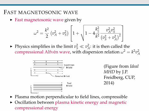
FAST MAGNETOSONIC WAVEI Fast magnetosonic wave given by

ω2 =k2

2(v2

A + v2S)1 +

√√√√1− 4k2‖

k2

v2Av2

S(v2

S + v2A

)2

I Physics simplifies in the limit v2

S � v2A: it is then called the

compressional Alfven wave, with dispersion relation ω2 = k2v2A

(Figure from IdealMHD by J.P.Freidberg, CUP,2014)

I Plasma motion perpendicular to field lines, compressibleI Oscillation between plasma kinetic energy and magnetic

compressional energy

SLOW MAGNETOSONIC WAVEI Slow magnetosonic wave given by

ω2 =k2

2(v2

A + v2S)1−

√√√√1− 4k2‖

k2

v2Av2

S(v2

S + v2A

)2

I Physics simplifies in the limit v2

S � v2A: it is then called the sound

wave, with dispersion relation ω2 = k2v2S

(Figure from IdealMHD by J.P.Freidberg, CUP,2014)

I Plasma motion parallel to field lines, compressibleI Oscillation between plasma kinetic energy and plasma internal

energy (plasma pressure)

COMMON MHD INSTABILITIES (I)

Interchange instability

(Figure from Plasma Physics and Fusion Energy by J.P. Freidberg, CUP, 2008)

COMMON MHD INSTABILITIES (II)

Ballooning instability(Figure from Plasma Physics and Fusion Energy by J.P. Freidberg, CUP, 2008)

COMMON MHD INSTABILITIES (III)

Kink instability

(Figure from Plasma Physics and Fusion Energy by J.P. Freidberg, CUP, 2008)

LINEAR STABILITY: ENERGY APPROACHI Change in potential energy: δW =

−→F ·−→dl

I Static equilibrium condition at x0: δW∣∣∣x=x0

= 0

I Stability

δ2W∣∣∣x=x0

> 0

δ2W∣∣∣x=x0

< 0

δ2W∣∣∣x=x0

= 0

IDEAL MHD ENERGY PRINCIPLE (I)I For historical reasons, the second variation is called δW in the

plasma physics jargonI A useful variational principle can be derived in ideal MHD,

called the energy principle , which takes the following form:

ω2 =δW(ξ)

K(ξ)

where

δW(ξ) = −12

∫ξ · F(ξ)dV

F (ξ) =1µ0{∇ × [∇× (ξ × B0)]} × B0 + (∇× B0)× [∇× (ξ × B0)]

+∇ (ξ · ∇p0 + γp0∇ · ξ)

K(ξ) =12

∫ρ|ξ|2dV

IDEAL MHD ENERGY PRINCIPLE (II)

ω2 =δW(ξ)

K(ξ)δW(ξ) = −1

2

∫ξ · F(ξ)dV

I Energy Principle: An ideal MHD equilibrium is stable if andonly if δW(ξ > 0 for all bounded ξ satisfying the boundaryconditions

I Energy principle very useful to prove instability of anequilibrium by coming up with a good guess for ξ that makesδW negative

I Formula also very helpful to calculate the ω2 numerically withhigh accuracy

POST SCRIPTUM: THE COURANT INSTITUTE OFMATHEMATICAL SCIENCES (CIMS) AT NYU

CIMS IN MANHATTAN

I Abel prize in 2005,2007, 2009 and 2015

I 18 members of theNational Academy ofSciences

5 members of theNational Academy ofEngineering

I Specialization in applied math, scientific computing,mathematical analysis

I Particular emphasis on Partial Differential Equations

I PhD programs in Mathematics, Atmosphere and Ocean Science,Computational Biology

I Masters of Science in Mathematics, Masters of Science inScientific Computing, Masters of Science in Data Science,Masters of Science in Math Finance

I ∼ 60 faculty∼ 100 PhD students

MFD DIVISION AT CIMS

I Founded by Harold Grad in 1954

I 3 faculty, 3 post-docs, 2 PhD students

I Work on MHD, wave propagation, kinetic modelsAnalytic “pen and paper” workDevelopment of new numerical solvers

I Collaboration with colleagues specialized in scientificcomputing, computational fluid dynamics, stochastic calculus,etc.

I Funding currently available for PhD students

I Feel free to contact me if you have any questions