introduction to numerical methods and matlab programming for...
TRANSCRIPT

Introduction to Numerical Methods
and Matlab Programming for Engineers
Todd Young and Martin J. MohlenkampDepartment of Mathematics
Ohio UniversityAthens, OH [email protected]
May 4, 2017

ii
Copyright c© 2008, 2009, 2011, 2014, 2016, 2017 Todd R. Young and Martin J. Mohlenkamp.Original edition 2004, by Todd R. Young.
This work is licensed under the Creative Commons Attribution-NonCommercial-ShareAlike4.0 International License. To view a copy of this license, visithttp://creativecommons.org/licenses/by-nc-sa/4.0/.

Preface
These notes were developed by the first author in the process of teaching a course on appliednumerical methods for Civil Engineering majors during 2002-2004 and was modified to includeMechanical Engineering in 2005. The materials have been periodically updated since then andunderwent a major revision by the second author in 2006-2007.
The main goals of these lectures are to introduce concepts of numerical methods and introduceMatlab in an Engineering framework. By this we do not mean that every problem is a “real life”engineering application, but more that the engineering way of thinking is emphasized throughoutthe discussion.
The philosophy of this book was formed over the course of many years. My father was a CivilEngineer and surveyor, and he introduced me to engineering ideas from an early age. At theUniversity of Kentucky I took most of the basic Engineering courses while getting a Bachelor’sdegree in Mathematics. Immediately afterward I completed a M.S. degree in Engineering Mechanicsat Kentucky. While working on my Ph.D. in Mathematics at Georgia Tech I taught all of theintroductory math courses for engineers. During my education, I observed that incorporation ofcomputation in coursework had been extremely unfocused and poor. For instance during my collegecareer I had to learn 8 different programming and markup languages on 4 different platforms plusnumerous other software applications. There was almost no technical help provided in the coursesand I wasted innumerable hours figuring out software on my own. A typical, but useless, inclusionof software has been (and still is in most calculus books) to set up a difficult ‘applied’ problem andthen add the line “write a program to solve” or “use a computer algebra system to solve”.
At Ohio University we have tried to take a much more disciplined and focused approach. The RussCollege of Engineering and Technology decided that Matlab should be the primary computationalsoftware for undergraduates. At about the same time members of the Department of Mathematicsproposed an 1804 project to bring Matlab into the calculus sequence and provide access to theprogram at nearly all computers on campus, including in the dorm rooms. The stated goal of thisproject was to make Matlab the universal language for computation on campus. That projectwas approved and implemented in the 2001-2002 academic year.
In these lecture notes, instruction on using Matlab is dispersed through the material on numericalmethods. In these lectures details about how to use Matlab are detailed (but not verbose) andexplicit. To teach programming, students are usually given examples of working programs and areasked to make modifications.
The lectures are designed to be used in a computer classroom, but could be used in a lecture format
iii
iv PREFACE
with students doing computer exercises afterward. The lectures are divided into four Parts with asummary provided at the end of each Part.
Todd Young
Dependencies
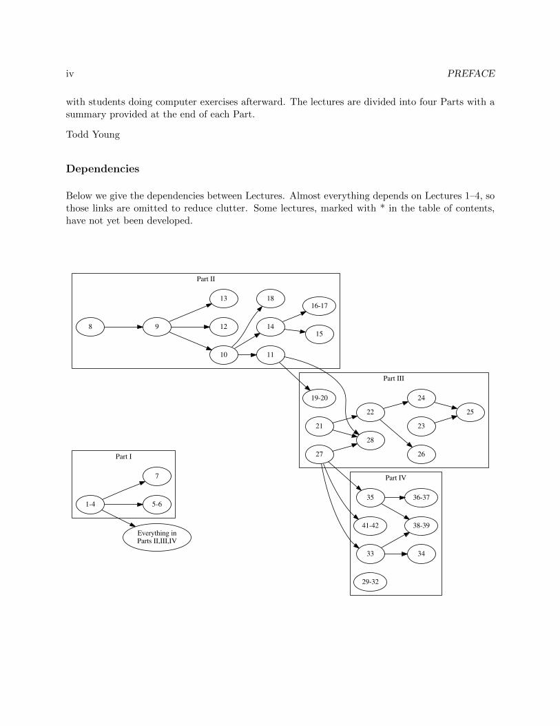
Below we give the dependencies between Lectures. Almost everything depends on Lectures 1–4, sothose links are omitted to reduce clutter. Some lectures, marked with * in the table of contents,have not yet been developed.
Part I
Part II
Part III
Part IV
1-4 5-6
7
Everything inParts II,III,IV
8 9
10
12
13
11
14
18
19-20
28
15
16-17
21
22
24
26
25
23
27
33
35
41-42
34
38-39
36-37
29-32

Contents
Preface iii
I Matlab and Solving Equations 1
Lecture 1. Vectors, Functions, and Plots in Matlab 2
Lecture 2. Matlab Programs 6
Lecture 3. Newton’s Method and Loops 10
Lecture 4. Controlling Error and Conditional Statements 14
Lecture 5. The Bisection Method and Locating Roots 18
Lecture 6. Secant Methods 22
Lecture 7. Symbolic Computations 25
Review of Part I 29
II Linear Algebra 33
Lecture 8. Matrices and Matrix Operations in Matlab 34
Lecture 9. Introduction to Linear Systems 39
Lecture 10. Some Facts About Linear Systems 43
Lecture 11. Accuracy, Condition Numbers and Pivoting 46
Lecture 12. LU Decomposition 50
Lecture 13. Nonlinear Systems - Newton’s Method 53
Lecture 14. Eigenvalues and Eigenvectors 57
Lecture 15. Vibrational Modes and Frequencies 60
Lecture 16. Numerical Methods for Eigenvalues 63
v
vi CONTENTS
Lecture 17. The QR Method* 67
Lecture 18. Iterative solution of linear systems* 69
Review of Part II 70
III Functions and Data 73
Lecture 19. Polynomial and Spline Interpolation 74
Lecture 20. Least Squares Fitting: Noisy Data 78
Lecture 21. Integration: Left, Right and Trapezoid Rules 81
Lecture 22. Integration: Midpoint and Simpson’s Rules 86
Lecture 23. Plotting Functions of Two Variables 90
Lecture 24. Double Integrals for Rectangles 93
Lecture 25. Double Integrals for Non-rectangles 97
Lecture 26. Gaussian Quadrature* 100
Lecture 27. Numerical Differentiation 101
Lecture 28. The Main Sources of Error 105
Review of Part III 108
IV Differential Equations 115
Lecture 29. Reduction of Higher Order Equations to Systems 116
Lecture 30. Euler Methods 120
Lecture 31. Higher Order Methods 124
Lecture 32. Multi-step Methods* 127
Lecture 33. ODE Boundary Value Problems and Finite Differences 128
Lecture 34. Finite Difference Method – Nonlinear ODE 132
Lecture 35. Parabolic PDEs - Explicit Method 135
Lecture 36. Solution Instability for the Explicit Method 140

CONTENTS vii
Lecture 37. Implicit Methods 143
Lecture 38. Insulated Boundary Conditions 147
Lecture 39. Finite Difference Method for Elliptic PDEs 152
Lecture 40. Convection-Diffusion Equations* 155
Lecture 41. Finite Elements 156
Lecture 42. Determining Internal Node Values 160
Review of Part IV 164
V Appendices 167
Lecture A. Glossary of Matlab Commands 168

viii CONTENTS

Part I
Matlab and Solving Equations
c©Copyright, Todd Young and Martin Mohlenkamp, Department of Mathematics, Ohio University, 2017
Lecture 1
Vectors, Functions, and Plots in Matlab
In these notes
will indicate commands to be entered at the Matlab prompt >> in the command window. You do nottype the symbol |.
Entering vectors
In Matlab, the basic objects are matrices, i.e. arrays of numbers. Vectors can be thought of as specialmatrices. A row vector is recorded as a 1×n matrix and a column vector is recorded as a m× 1 matrix. Toenter a row vector in Matlab, type the following in the command window:
v = [0 1 2 3]
and press enter. Matlab will print out the row vector. To enter a column vector type
u = [9; 10; 11; 12; 13]
You can access an entry in a vector with
u(2)
and change the value of that entry with
u(2)=47
You can extract a slice out of a vector with
u(2:4)
You can change a row vector into a column vector, and vice versa easily in Matlab using
w = v’
(This is called transposing the vector and we call ’ the transpose operator.) There are also useful shortcutsto make vectors such as
2

3
x = -1:.1:1
y = linspace (0,1,11)
Basic Formatting
To make Matlab put fewer blank lines in its output, enter
format compact
To make Matlab display more digits, enter
format long
Note that this does not change the number of digits Matlab is using in its calculations; it only changeswhat is diplayed.
Plotting Data
Consider the data in Table 1.1.1 We can enter this data into Matlab with the following commands entered
T (C) 5 20 30 50 55µ 0.08 0.015 0.009 0.006 0.0055
Table 1.1: Viscosity of a liquid as a function of temperature.
in the command window:
x = [ 5 20 30 50 55 ]
y = [ 0.08 0.015 0.009 0.006 0.0055]
Entering the name of the variable retrieves its current values. For instance
x
y
We can plot data in the form of vectors using the plot command:
plot(x,y)
This will produce a graph with the data points connected by lines. If you would prefer that the data pointsbe represented by symbols you can do so. For instance
plot(x,y,’*’)
plot(x,y,’o’)
plot(x,y,’.’)
1Adapted from Ayyup &McCuen 1996, p.174.

4 LECTURE 1. VECTORS, FUNCTIONS, AND PLOTS IN MATLAB
Data as a Representation of a Function
A major theme in this course is that often we are interested in a certain function y = f(x), but the onlyinformation we have about this function is a discrete set of data (xi, yi). Plotting the data, as we didabove, can be thought of envisioning the function using just the data. We will find later that we can also doother things with the function, like differentiating and integrating, just using the available data. Numericalmethods, the topic of this course, means doing mathematics by computer. Since a computer can only storea finite amount of information, we will almost always be working with a finite, discrete set of values of thefunction (data), rather than a formula for the function.
Built-in Functions
If we wish to deal with formulas for functions, Matlab contains a number of built-in functions, includingall the usual functions, such as sin( ), exp( ), etc.. The meaning of most of these is clear. The dependentvariable (input) always goes in parentheses in Matlab. For instance
sin(pi)
should return the value of sinπ, which is of course 0 and
exp (0)
will return e0 which is 1. More importantly, the built-in functions can operate not only on single numbersbut on vectors. For example
x = linspace (0,2*pi ,40)
y = sin(x)
plot(x,y)
will return a plot of sinx on the interval [0, 2π]
Some of the built-in functions in Matlab include: cos( ), tan( ), sinh( ), cosh( ), log( ) (naturallogarithm), log10( ) (log base 10), asin( ) (inverse sine), acos( ), atan( ). To find out more about afunction, use the help command; try
help plot
User-Defined Anonymous Functions
If we wish to deal with a function that is a combination of the built-in functions, Matlab has a couple ofways for the user to define functions. One that we will use a lot is the anonymous function, which is a wayto define a function in the command window. The following is a typical anonymous function:
f = @(x) 2*x.^2 - 3*x + 1
This produces the function f(x) = 2x2 − 3x+ 1. To obtain a single value of this function enter
y = f(2.23572)

5
Just as for built-in functions, the function f as we defined it can operate not only on single numbers but onvectors. Try the following:
x = -2:.2:2
y = f(x)
This is an example of vectorization, i.e. putting several numbers into a vector and treating the vector all atonce, rather than one component at a time, and is one of the strengths of Matlab. The reason f(x) workswhen x is a vector is because we represented x2 by x.^2. The . turns the exponent operator ^ into entry-wiseexponentiation, so that [-2 -1.8 -1.6].^2 means [(−2)2, (−1.8)2, (−1.6)2] and yields [4 3.24 2.56]. Incontrast, [-2 -1.8 -1.6]^2 means the matrix product [−2,−1.8,−1.6][−2,−1.8,−1.6] and yields only anerror. The . is needed in .^, .*, and ./. It is not needed when you * or / by a scalar or for +.
The results can be plotted using the plot command, just as for data:
plot(x,y)
Notice that before plotting the function, we in effect converted it into data. Plotting on any machine alwaysrequires this step.
Exercises
1.1 Find a table of data in an engineering or science textbook or website. Input it as vectors and plot it.Use the insert icon to label the axes and add a title to your graph. Turn in the graph. Indicate whatthe data is and properly reference where it came from.
1.2 Find a function formula in an engineering or science textbook or website. Make an anonymous functionthat produces that function. Plot it on a physically relevant domain. Label the axes and add a titleto your graph. Turn in the graph and write on the page the Matlab command for the anonymousfunction. Indicate what the function means and properly reference where it came from.

Lecture 2
Matlab Programs
In Matlab, programs may be written and saved in files with a suffix .m called M-files. There are two typesof M-file programs: functions and scripts.
Function Programs
Begin by clicking on the new document icon in the top left of the Matlab window (it looks like an emptysheet of paper).
In the document window type the following:
function y = myfunc(x)
y = 2*x.^2 - 3*x + 1;
end
Save this file as: myfunc.m in your working directory. This file can now be used in the command windowjust like any predefined Matlab function; in the command window enter:
x = -2:.1:2; % Produces a vector of x values
y = myfunc(x); % Produces a vector of y values
plot(x,y)
Note that the fact we used x and y in both the function program and in the command window was just acoincidence. In fact, it is the name of the file myfunc.m that actually mattered, not what anything in it wascalled. We could just as well have made the function
function nonsense = yourfunc(inputvector)
nonsense = 2* inputvector .^2 - 3* inputvector + 1;
end
Look back at the program. All function programs are like this one, the essential elements are:
• Begin with the word function.
• There is an input and an output.
• The output, name of the function and the input must appear in the first line.
• The body of the program must assign a value to the output variable(s).
6
7
• The program cannot access variables in the current workspace unless they are input.
• Internal variables inside a function do not appear in the current workspace.
Functions can have multiple inputs, which are separated by commas. For example:
function y = myfunc2d(x,p)
y = 2*x.^p - 3*x + 1;
end
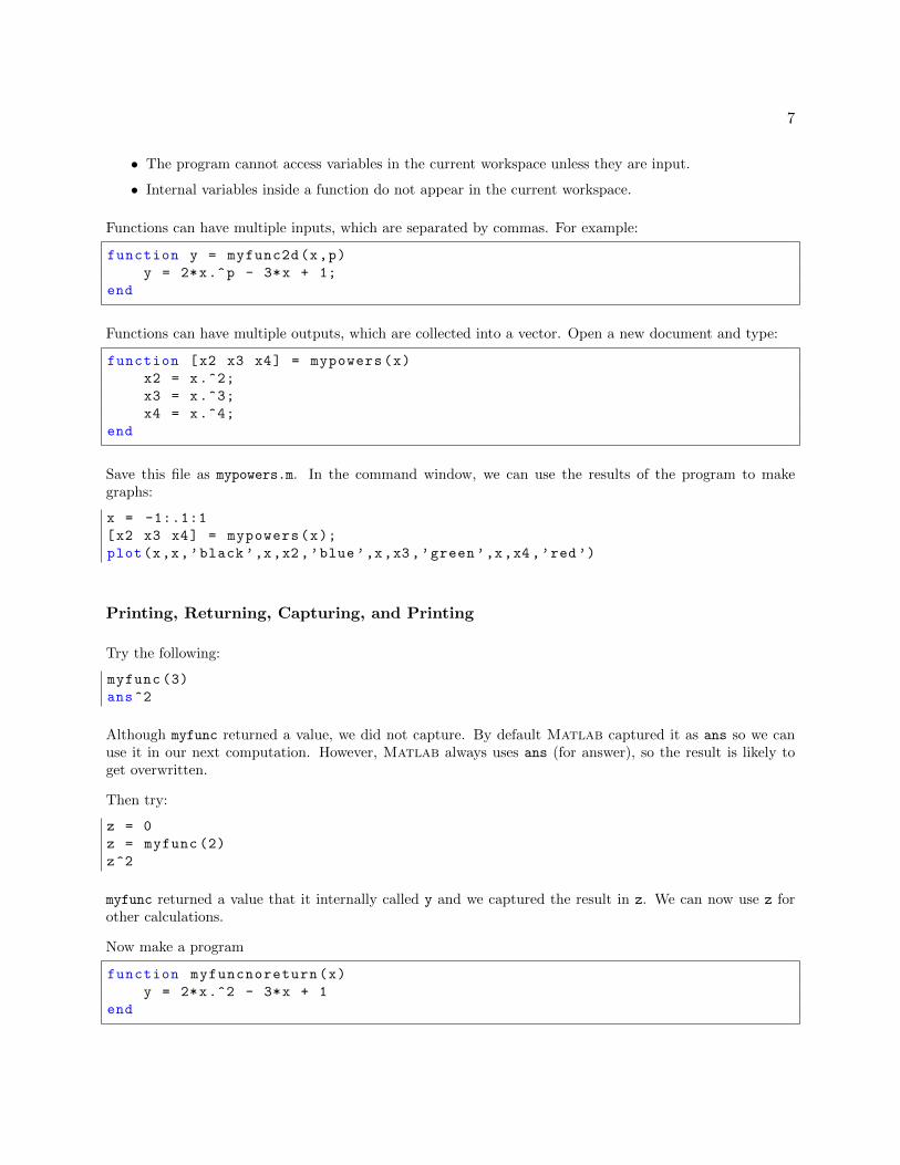
Functions can have multiple outputs, which are collected into a vector. Open a new document and type:
function [x2 x3 x4] = mypowers(x)
x2 = x.^2;
x3 = x.^3;
x4 = x.^4;
end
Save this file as mypowers.m. In the command window, we can use the results of the program to makegraphs:
x = -1:.1:1
[x2 x3 x4] = mypowers(x);
plot(x,x,’black’,x,x2 ,’blue’,x,x3 ,’green’,x,x4 ,’red’)
Printing, Returning, Capturing, and Printing
Try the following:
myfunc (3)
ans^2
Although myfunc returned a value, we did not capture. By default Matlab captured it as ans so we canuse it in our next computation. However, Matlab always uses ans (for answer), so the result is likely toget overwritten.
Then try:
z = 0
z = myfunc (2)
z^2
myfunc returned a value that it internally called y and we captured the result in z. We can now use z forother calculations.
Now make a program
function myfuncnoreturn(x)
y = 2*x.^2 - 3*x + 1
end

8 LECTURE 2. MATLAB PROGRAMS
and try:
myfuncnoreturn (4)
ans^2
y^2
Although the value of y was printed within the function, it was not returned, so neither the value of y northe value of ans was changed. Thus we cannot use the result from the function.
In general, the best way to use a function is to capture the result it returns and then use or print this result.Printing within functions is bad form; however, for understanding what is happening within a function it isuseful to print, so many functions in this book do print.
Script Programs
Matlab uses a second type of program that differs from a function program in several ways, namely:
• There are no inputs and outputs.
• A script program may use, create and change variables in the current workspace (the variables usedby the command window).
Below is a script program that accomplishes the same thing as the function program plus the commands inthe previous section:
x2 = x.^2;
x3 = x.^3;
x4 = x.^4;
plot(x,x,’black’,x,x2 ,’blue’,x,x3 ,’green’,x,x4 ,’red’)
Type this program into a new document and save it as mygraphs.m. In the command window enter:
x = -1:.1:1;
mygraphs
Note that the program used the variable x in its calculations, even though x was defined in the commandwindow, not in the program.
Many people use script programs for routine calculations that would require typing more than one commandin the command window. They do this because correcting mistakes is easier in a program than in thecommand window.
Program Comments
For programs that have more than a couple of lines it is important to include comments. Comments allowother people to know what your program does and they also remind yourself what your program does if youset it aside and come back to it later. It is best to include comments not only at the top of a program, butalso with each section. In Matlab anything that comes in a line after a % is a comment.

9
For a function program, the comments should at least give the purpose, inputs, and outputs. A properlycommented version of the function with which we started this section is:
function y = myfunc(x)
% Computes the function 2x^2 -3x +1
% Input: x -- a number or vector;
% for a vector the computation is elementwise
% Output: y -- a number or vector of the same size as x
y = 2*x.^2 - 3*x + 1;
end
For a script program it is often helpful to include the name of the program at the beginning. For example:
% mygraphs
% plots the graphs of x, x^2, x^3, and x^4
% on the interval [-1,1]
% fix the domain and evaluation points
x = -1:.1:1;
% calculate powers
% x1 is just x
x2 = x.^2;
x3 = x.^3;
x4 = x.^4;
% plot each of the graphs
plot(x,x,’+-’,x,x2 ,’x-’,x,x3 ,’o-’,x,x4 ,’--’)
The Matlab command help prints the first block of comments from a file. If we save the above asmygraphs.m and then do
help mygraphs
it will print into the command window:
mygraphs
plots the graphs of x, x^2, x^3, and x^4
on the interval [-1,1]
Exercises
2.1 Write a well-commented function program for the function x2e−x2
, using entry-wise operations (suchas .* and .^). To get ex use exp(x). Plot the function on [−5, 5] using enough points to make thegraph smooth. Turn in printouts of the program and the graph.
2.2 Write a well-commented script program that graphs the functions sinx, sin 2x, sin 3x, sin 4x, sin 5xand sin 6x on the interval [0, 2π] on one plot. (π is pi in Matlab.) Use a sufficiently small step sizeto make all the graphs smooth. Turn in the program and the graph.

Lecture 3
Newton’s Method and Loops
Solving equations numerically
For the next few lectures we will focus on the problem of solving an equation:
f(x) = 0. (3.1)
As you learned in calculus, the final step in many optimization problems is to solve an equation of this formwhere f is the derivative of a function, F , that you want to maximize or minimize. In real engineeringproblems the functions, f , you wish to find roots for can come from a large variety of sources, includingformulas, solutions of differential equations, experiments, or simulations.
Newton iterations
We will denote an actual solution of equation (3.1) by x∗. There are three methods which you may havediscussed in Calculus: the bisection method, the secant method and Newton’s method. All three depend onbeginning close (in some sense) to an actual solution x∗.
Recall Newton’s method. You should know that the basis for Newton’s method is approximation of a functionby its linearization at a point, i.e.
f(x) ≈ f(x0) + f ′(x0)(x− x0). (3.2)
Since we wish to find x so that f(x) = 0, set the left hand side (f(x)) of this approximation equal to 0 andsolve for x to obtain:
x ≈ x0 −f(x0)
f ′(x0). (3.3)
We begin the method with the initial guess x0, which we hope is fairly close to x∗. Then we define a sequenceof points x0, x1, x2, x3, . . . from the formula:
xi+1 = xi −f(xi)
f ′(xi), (3.4)
which comes from (3.3). If f(x) is reasonably well-behaved near x∗ and x0 is close enough to x∗, then it isa fact that the sequence will converge to x∗ and will do it very quickly.
The loop: for ... end
In order to do Newton’s method, we need to repeat the calculation in (3.4) a number of times. This isaccomplished in a program using a loop, which means a section of a program which is repeated. The
10

11
simplest way to accomplish this is to count the number of times through. In Matlab, a for ... end
statement makes a loop as in the following simple function program:
function S = mysum(n)
% Gives the sum of the first n integers
% Input: n
% Output: the sum
S = 0; % start at zero
% The loop:
for i = 1:n % do n times
S = S + i; % add the current integer
end % end of the loop
end
Call this function in the command window as:
mysum (100)
The result will be the sum of the first 100 integers. All for ... end loops have the same format, it beginswith for, followed by an index (i) and a range of numbers (1:n). Then come the commands that are to berepeated. Last comes the end command.
Loops are one of the main ways that computers are made to do calculations that humans cannot. Anycalculation that involves a repeated process is easily done by a loop.
Now let’s do a program that does n steps (iterations) of Newton’s method. We will need to input thefunction, its derivative, the initial guess, and the number of steps. The output will be the final value of x,i.e. xn. If we are only interested in the final approximation, not the intermediate steps, which is usually thecase in the real world, then we can use a single variable x in the program and change it at each step:
function x = mynewton(f,f1,x0,n)
% Solves f(x) = 0 by doing n steps of Newton ’s method starting at x0.
% Inputs: f -- the function
% f1 -- it ’s derivative
% x0 -- starting guess , a number
% n -- the number of steps to do
% Output: x -- the approximate solution
x = x0; % set x equal to the initial guess x0
for i = 1:n % Do n times
x = x - f(x)/f1(x) % Newton ’s formula , prints x too
end
end
In the command window set to print more digits via
format long
and to not print blank lines via
format compact

12 LECTURE 3. NEWTON’S METHOD AND LOOPS
Then define a function: f(x) = x3 − 5 i.e.
f = @(x) x^3 - 5
and define f1 to be its derivative, i.e.
f1 = @(x) 3*x^2
Then run mynewton on this function. By trial and error, what is the lowest value of n for which the programconverges (stops changing). By simple algebra, the true root of this function is 3
√5. How close is the
program’s answer to the true value?
Convergence
Newton’s method converges rapidly when f ′(x∗) is nonzero and finite, and x0 is close enough to x∗ that thelinear approximation (3.2) is valid. Let us take a look at what can go wrong.
For f(x) = x1/3 we have x∗ = 0 but f ′(x∗) =∞. If you try
f = @(x) x^(1/3)
f1 = @(x) (1/3)*x^( -2/3)
x = mynewton(f,f1 ,0.1 ,10)
then x explodes.
For f(x) = x2 we have x∗ = 0 but f ′(x∗) = 0. If you try
f = @(x) x^2
f1 = @(x) 2*x
x = mynewton(f,f1 ,1 ,10)
then x does converge to 0, but not that rapidly.
If x0 is not close enough to x∗ that the linear approximation (3.2) is valid, then the iteration (3.4) givessome x1 that may or may not be any better than x0. If we keep iterating, then either
• xn will eventually get close to x∗ and the method will then converge (rapidly), or
• the iterations will not approach x∗.
13
Exercises
3.1 Enter: format long. Use mynewton on the function f(x) = x5 − 7, with x0 = 2. By trial and error,what is the lowest value of n for which the program converges (stops changing). Compute the error,which is how close the program’s answer is to the true value. Compute the residual, which is theprogram’s answer plugged into f . (See the next section for discussion.) Are the error and residualzero?
3.2 Suppose a ball is dropped from a height of 2 meters onto a hard surface and the coefficient of restitutionof the collision is .9 (see Wikipedia for an explanation). Write a well-commented script program tocalculate the total distance the ball has traveled when it hits the surface for the n-th time. Enter:format long. By trial and error approximate how large n must be so that total distance stopschanging. Turn in the program and a brief summary of the results.
3.3 For f(x) = x3 − 4, perform 3 iterations of Newton’s method with starting point x0 = 2. (On paper,but use a calculator.) Calculate the solution (x∗ = 41/3) on a calculator and find the errors andpercentage errors of x0, x1, x2 and x3. Use enough digits so that you do not falsely conclude the erroris zero. Put the results in a table.
Lecture 4
Controlling Error and Conditional Statements
Measuring error and the Residual
If we are trying to find a numerical solution of an equation f(x) = 0, then there are a few different ways wecan measure the error of our approximation. The most direct way to measure the error would be as
Error at step n = en = xn − x∗
where xn is the n-th approximation and x∗ is the true value. However, we usually do not know the value ofx∗, or we wouldn’t be trying to approximate it. This makes it impossible to know the error directly, and sowe must be more clever.
One possible strategy, that often works, is to run a program until the approximation xn stops changing.The problem with this is that it sometimes doesn’t work. Just because the program stop changing does notnecessarily mean that xn is close to the true solution.
For Newton’s method we have the following principle: At each step the number of significant digitsroughly doubles. While this is an important statement about the error (since it means Newton’s methodconverges really quickly), it is somewhat hard to use in a program.
Rather than measure how close xn is to x∗, in this and many other situations it is much more practical tomeasure how close the equation is to being satisfied, in other words, how close yn = f(xn) is to 0. We willuse the quantity rn = f(xn)− 0, called the residual, in many different situations. Most of the time we onlycare about the size of rn, so we use the absolute value of the residual as a measure of how close the solutionis to solving the problem:
|rn| = |f(xn)|.
The if ... end statement
If we have a certain tolerance for |rn| = |f(xn)|, then we can incorporate that into our Newton methodprogram using an if ... end statement:
function x = mynewton(f,f1,x0,n,tol)
% Solves f(x) = 0 by doing n steps of Newton ’s method starting at x0.
% Inputs: f -- the function
% f1 -- it ’s derivative
% x0 -- starting guess , a number
% tol -- desired tolerance , prints a warning if |f(x)|>tol
14

15
% Output: x -- the approximate solution
x = x0; % set x equal to the initial guess x0
for i = 1:n % Do n times
x = x - f(x)/f1(x) % Newton ’s formula
end
r = abs(f(x))
if r > tol
warning(’The desired accuracy was not attained ’)
end
end
In this program if checks if abs(y) > tol is true or not. If it is true then it does everything between thereand end. If not true, then it skips ahead to end.
In the command window define a function and its derivative:
f = @(x) x^3-5
f1 = @(x) 3*x^2
Then use the program with n = 3, tol = .01, and x0 = 2. Next, change tol to 10−10 and repeat.
The loop: while ... end
While the previous program will tell us if it worked or not, we still have to input n, the number of steps totake. Even for a well-behaved problem, if we make n too small then the tolerance will not be attained andwe will have to go back and increase it, or, if we make n too big, then the program will take more steps thannecessary.
One way to control the number of steps taken is to iterate until the residual |rn| = |f(x)| = |y| is smallenough. In Matlab this is easily accomplished with a while ... end loop.
function x = mynewtontol(f,f1,x0,tol)
% Solves f(x) = 0 using Newton ’s method until |f(x)| < tol.
% Inputs: f -- the function
% f1 -- it ’s derivative
% x0 -- starting guess , a number
% tol -- desired tolerance , runs until |f(x)|<tol
% Output: x -- the approximate solution
x = x0; % set x equal to the initial guess x0
y = f(x);
while abs(y) > tol % Do until the tolerence is reached.
x = x - y/f1(x) % Newton ’s formula
y = f(x)
end
end
The statement while ... end is a loop, similar to for ... end, but instead of going through the loop afixed number of times it keeps going as long as the statement abs(y) > tol is true.
16 LECTURE 4. CONTROLLING ERROR AND CONDITIONAL STATEMENTS
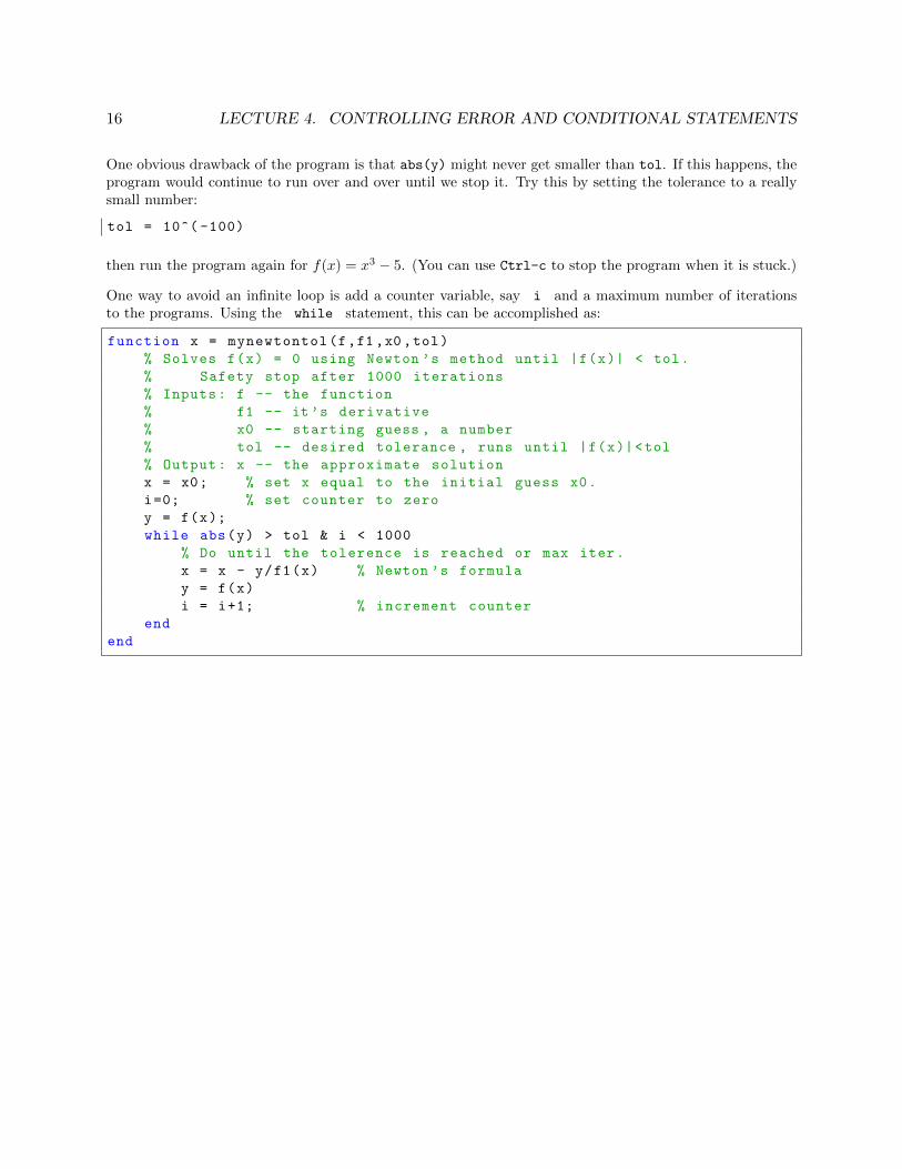
One obvious drawback of the program is that abs(y) might never get smaller than tol. If this happens, theprogram would continue to run over and over until we stop it. Try this by setting the tolerance to a reallysmall number:
tol = 10^( -100)
then run the program again for f(x) = x3 − 5. (You can use Ctrl-c to stop the program when it is stuck.)
One way to avoid an infinite loop is add a counter variable, say i and a maximum number of iterationsto the programs. Using the while statement, this can be accomplished as:
function x = mynewtontol(f,f1,x0,tol)
% Solves f(x) = 0 using Newton ’s method until |f(x)| < tol.
% Safety stop after 1000 iterations
% Inputs: f -- the function
% f1 -- it ’s derivative
% x0 -- starting guess , a number
% tol -- desired tolerance , runs until |f(x)|<tol
% Output: x -- the approximate solution
x = x0; % set x equal to the initial guess x0.
i=0; % set counter to zero
y = f(x);
while abs(y) > tol & i < 1000
% Do until the tolerence is reached or max iter.
x = x - y/f1(x) % Newton ’s formula
y = f(x)
i = i+1; % increment counter
end
end

17
Exercises
4.1 In Calculus we learn that a geometric series has an exact sum
∞∑i=0
ri =1
1− r,
provided that |r| < 1. For instance, if r = .5 then the sum is exactly 2. Below is a script programthat lacks one line as written. Put in the missing command and then use the program to verify theresult above. How many steps does it take? How close is the answer to 2?
% Computes a geometric series until it seems to converge
format long
format compact
r = .5;
Snew = 0; % start sum at 0
Sold = -1; % set Sold to trick while the first time
i = 0; % count iterations
while Snew > Sold % is the sum still changing?
Sold = Snew; % save previous value to compare to
Snew = Snew + r^i;
i=i+1;
Snew % prints the final value.
i % prints the # of iterations.
Add a line at the end of the program to compute the relative error of Snew versus the exact value.Run the script for r = 0.9, 0.99, 0.999, 0.9999, 0.99999, and 0.999999. In a table, report the numberof iterations needed and the relative error for each r.
4.2 Modify your program from exercise 3.2 to compute the total distance traveled by the ball while itsbounces are at least 1 millimeter high. Use a while loop to decide when to stop summing; do not usea for loop or trial and error. Turn in your modified program and a brief summary of the results.

Lecture 5
The Bisection Method and Locating Roots
Bisecting and the if ... else ... end statement
Recall the bisection method. Suppose that c = f(a) < 0 and d = f(b) > 0. If f is continuous, then obviouslyit must be zero at some x∗ between a and b. The bisection method then consists of looking half way betweena and b for the zero of f , i.e. let x = (a + b)/2 and evaluate y = f(x). Unless this is zero, then from thesigns of c, d and y we can decide which new interval to subdivide. In particular, if c and y have the samesign, then [x, b] should be the new interval, but if c and y have different signs, then [a, x] should be the newinterval. (See Figure 5.1.)
x0x1 x2a0 b0
a1 b1
a2 b2u
uu
u
Figure 5.1: The bisection method.
Deciding to do different things in different situations in a program is called flow control. The most commonway to do this is the if ... else ... end statement which is an extension of the if ... end statementwe have used already.
Bounding the Error
One good thing about the bisection method, that we don’t have with Newton’s method, is that we alwaysknow that the actual solution x∗ is inside the current interval [a, b], since f(a) and f(b) have different signs.This allows us to be sure about what the maximum error can be. Precisely, the error is always less than halfof the length of the current interval [a, b], i.e.
Absolute Error = |x− x∗| < (b− a)/2,
where x is the center point between the current a and b.
18

19
The following function program (also available on the webpage) does n iterations of the bisection methodand returns not only the final value, but also the maximum possible error:
function [x e] = mybisect(f,a,b,n)
% function [x e] = mybisect(f,a,b,n)
% Does n iterations of the bisection method for a function f
% Inputs: f -- a function
% a,b -- left and right edges of the interval
% n -- the number of bisections to do.
% Outputs: x -- the estimated solution of f(x) = 0
% e -- an upper bound on the error
% evaluate at the ends and make sure there is a sign change
c = f(a); d = f(b);
if c*d > 0.0
error(’Function has same sign at both endpoints.’)
end
disp(’ x y’)
for i = 1:n
% find the middle and evaluate there
x = (a + b)/2;
y = f(x);
disp([ x y])
if y == 0.0 % solved the equation exactly
e = 0;
break % jumps out of the for loop
end
% decide which half to keep , so that the signs at the ends differ
if c*y < 0
b=x;
else
a=x;
end
end
% set the best estimate for x and the error bound
x = (a + b)/2;
e = (b-a)/2;
end
Another important aspect of bisection is that it always works. We saw that Newton’s method can fail toconverge to x∗ if x0 is not close enough to x∗. In contrast, the current interval [a, b] in bisection will alwaysget decreased by a factor of 2 at each step and so it will always eventually shrink down as small as you wantit.
Locating a root
The bisection method and Newton’s method are both used to obtain closer and closer approximations of asolution, but both require starting places. The bisection method requires two points a and b that have a root

20 LECTURE 5. THE BISECTION METHOD AND LOCATING ROOTS
between them, and Newton’s method requires one point x0 which is reasonably close to a root. How do youcome up with these starting points? It depends. If you are solving an equation once, then the best thing todo first is to just graph it. From an accurate graph you can see approximately where the graph crosses zero.
There are other situations where you are not just solving an equation once, but have to solve the sameequation many times, but with different coefficients. This happens often when you are developing softwarefor a specific application. In this situation the first thing you want to take advantage of is the natural domainof the problem, i.e. on what interval is a solution physically reasonable. If that is known, then it is easyto get close to the root by simply checking the sign of the function at a fixed number of points inside theinterval. Whenever the sign changes from one point to the next, there is a root between those points. Thefollowing program will look for the roots of a function f on a specified interval [a0, b0].
function [a,b] = myrootfind(f,a0,b0)
% function [a,b] = myrootfind(f,a0,b0)
% Looks for subintervals where the function changes sign
% Inputs: f -- a function
% a0 -- the left edge of the domain
% b0 -- the right edge of the domain
% Outputs: a -- an array , giving the left edges of subintervals
% on which f changes sign
% b -- an array , giving the right edges of the subintervals
n = 1001; % number of test points to use
a = []; % start empty array
b = [];
% split the interval into n-1 intervals and evaluate at the break points
x = linspace(a0,b0,n);
y = f(x);
% loop through the intervals
for i = 1:(n-1)
if y(i)*y(i+1) < 0 % The sign changed , record it
a = [a x(i)];
b = [b x(i+1)];
end
end
if size(a,1) == 0
warning(’no roots were found’)
end
end
The final situation is writing a program that will look for roots with no given information. This is a difficultproblem and one that is not often encountered in engineering applications.
Once a root has been located on an interval [a, b], these a and b can serve as the beginning points for thebisection and secant methods (see the next section). For Newton’s method one would want to choose x0between a and b. One obvious choice would be to let x0 be the bisector of a and b, i.e. x0 = (a+ b)/2. Aneven better choice would be to use the secant method to choose x0.

21
Exercises
5.1 Modify mybisect to solve until the absolute error is bounded by a given tolerance. Use a while loopto do this. Run your program on the function f(x) = 2x3 + 3x− 1 with starting interval [0, 1] and atolerance of 10−8. How many steps does the program use to achieve this tolerance? (You can countthe step by adding 1 to a counting variable i in the loop of the program.) How big is the final residualf(x)? Turn in your program and a brief summary of the results.
5.2 Perform 3 iterations of the bisection method on the function f(x) = x3 − 4, with starting interval[1, 3]. (On paper, but use a calculator.) Calculate the errors and percentage errors of x0, x1, x2, andx3. Compare the errors with those in exercise 3.3.
Lecture 6
Secant Methods
In this lecture we introduce two additional methods to find numerical solutions of the equation f(x) = 0.Both of these methods are based on approximating the function by secant lines just as Newton’s methodwas based on approximating the function by tangent lines.
The Secant Method
The secant method requires two initial approximations x0 and x1, preferably both reasonably close to thesolution x∗. From x0 and x1 we can determine that the points (x0, y0 = f(x0)) and (x1, y1 = f(x1)) bothlie on the graph of f . Connecting these points gives the (secant) line
y − y1 =y1 − y0x1 − x0
(x− x1) .
Since we want f(x) = 0, we set y = 0, solve for x, and use that as our next approximation. Repeating thisprocess gives us the iteration
xi+1 = xi −xi − xi−1yi − yi−1
yi (6.1)
with yi = f(xi). See Figure 6.1 for an illustration.
For example, suppose f(x) = x4 − 5, which has a solution x∗ = 4√
5 ≈ 1.5. Choose x0 = 1 and x1 = 2 asinitial approximations. Next we have that y0 = f(1) = −4 and y1 = f(2) = 11. We may then calculate x2from the formula (6.1):
x2 = 2− 2− 1
11− (−4)11 =
19
15≈ 1.2666....
Pluggin x2 = 19/15 into f(x) we obtain y2 = f(19/15) ≈ −2.425758.... In the next step we would use x1 = 2and x2 = 19/15 in the formula (6.1) to find x3 and so on.
Below is a program for the secant method. Notice that it requires two input guesses x0 and x1, but it doesnot require the derivative to be input.
22

23
uxi
u
xi−1xi+1
Figure 6.1: The secant method in the case where the root is bracketed.
function x = mysecant(f,x0,x1,n)
% Solves f(x) = 0 by doing n steps of the secant method
% starting with x0 and x1.
% Inputs: f -- the function
% x0 -- starting guess , a number
% x1 -- second starting guess
% n -- the number of steps to do
% Output: x -- the approximate solution
y0 = f(x0);
y1 = f(x1);
for i = 1:n % Do n times
x = x1 - (x1 -x0)*y1/(y1 -y0) % secant formula.
y=f(x) % y value at the new approximate solution.
% Move numbers to get ready for the next step
x0=x1;
y0=y1;
x1=x;
y1=y;
end
end
The Regula Falsi (False Position) Method
The Regula Falsi method is a combination of the secant method and bisection method. As in the bisectionmethod, we have to start with two approximations a and b for which f(a) and f(b) have different signs. Asin the secant method, we follow the secant line to get a new approximation, which gives a formula similar
24 LECTURE 6. SECANT METHODS
to (6.1),
x = b− b− af(b)− f(a)
f(b) .
Then, as in the bisection method, we check the sign of f(x); if it is the same as the sign of f(a) then xbecomes the new a and otherwise let x becomes the new b. Note that in general either a → x∗ or b → x∗
but not both, so b− a 6→ 0. For example, for the function in Figure 6.1, a→ x∗ but b would never move.
Convergence
If we can begin with a good choice x0, then Newton’s method will converge to x∗ rapidly. The secant methodis a little slower than Newton’s method and the Regula Falsi method is slightly slower than that. However,both are still much faster than the bisection method.
If we do not have a good starting point or interval, then the secant method, just like Newton’s method, canfail altogether. The Regula Falsi method, just like the bisection method, always works because it keeps thesolution inside a definite interval.
Simulations and Experiments
Although Newton’s method converges faster than any other method, there are contexts when it is notconvenient, or even impossible. One obvious situation is when it is difficult to calculate a formula for f ′(x)even though one knows the formula for f(x). This is often the case when f(x) is not defined explicitly,but implicitly. There are other situations, which are very common in engineering and science, where evena formula for f(x) is not known. This happens when f(x) is the result of experiment or simulation ratherthan a formula. In such situations, the secant method is usually the best choice.
Exercises
6.1 Perform 3 iterations of the secant method on the function f(x) = x3− 4, with starting points x−1 = 1and x0 = 3. (On paper, but use a calculator.) Calculate the errors and percentage errors of x1, x2,and x3. Compare the errors with those in exercise 3.3.
6.2 Perform 3 iterations of the Regula Falsi method on the function f(x) = x3 − 4, with starting interval[1, 3]. (On paper, but use a calculator.) Calculate the errors and percentage errors of x1, x2, and x3.Compare the errors with those in exercises 3.3 and 5.2.
6.3 Modify the program mysecant.m to iterate until the absolute value of the residual is less than a giventolerance. (Let tol be an input instead of n.) Modify the comments appropriately. Turn in theprogram.

Lecture 7
Symbolic Computations
The focus of this course is on numerical computations, i.e. calculations, usually approximations, with floatingpoint numbers. However, Matlab can also do symbolic computations, which means exact calculations usingsymbols as in Algebra or Calculus.
Note: To do symbolic computations in Matlab one must have the Symbolic Toolbox.
Defining functions and basic operations
Before doing any symbolic computation, one must declare the variables used to be symbolic:
syms x y
A function is defined by simply typing the formula:
f = cos(x) + 3*x^2
Note that coefficients must be multiplied using *. To find specific values, you must use the command subs:
subs(f,pi)
This command stands for substitute, it substitutes π for x in the formula for f . If we define another function:
g = exp(-y^2)
then we can compose the functions:
h = compose(g,f)
i.e. h(x) = g(f(x)). Since f and g are functions of different variables, their product must be a function oftwo variables:
k = f*g
subs(k,[x,y],[0,1])
We can do simple calculus operations, like differentiation:
f1 = diff(f)
k1x = diff(k,x)
25
26 LECTURE 7. SYMBOLIC COMPUTATIONS
indefinite integrals (antiderivatives):
F = int(f)
and definite integrals:
int(f,0,2*pi)
To change a symbolic answer into a numerical answer, use the double command which stands for doubleprecision, (not times 2):
double(ans)
Note that some antiderivatives cannot be found in terms of elementary functions; for some of these theantiderivative can be expressed in terms of special functions:
G = int(g)
and for others Matlab does the best it can:
int(h)
For definite integrals that cannot be evaluated exactly, Matlab does nothing and prints a warning:
int(h,0,1)
We will see later that even functions that don’t have an antiderivative can be integrated numerically. Youcan change the last answer to a numerical answer using:
double(ans)
Plotting a symbolic function can be done as follows:
ezplot(f)
or the domain can be specified:
ezplot(g,-10,10)
ezplot(g,-2,2)
To plot a symbolic function of two variables use:
ezsurf(k)
It is important to keep in mind that even though we have defined our variables to be symbolic variables,plotting can only plot a finite set of points. For intance:
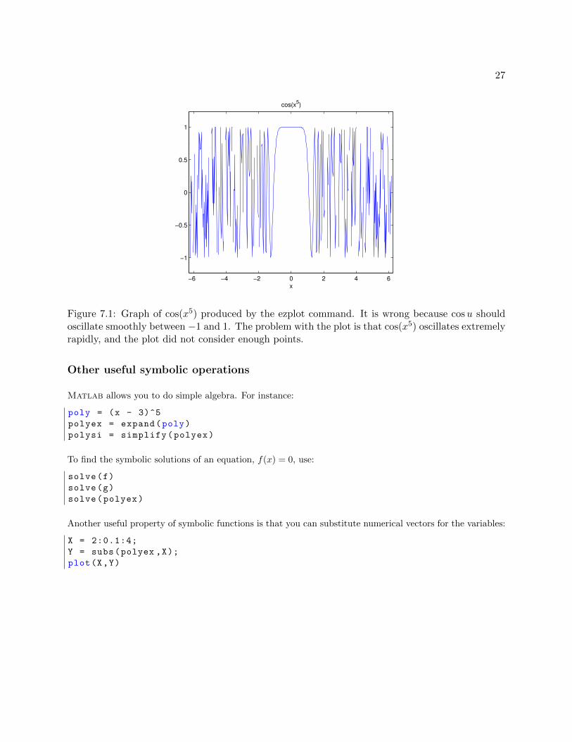
ezplot(cos(x^5))
will produce the plot in Figure 7.1, which is clearly wrong, because it does not plot enough points.
27
−6 −4 −2 0 2 4 6
−1
−0.5
0
0.5
1
x
cos(x5)
Figure 7.1: Graph of cos(x5) produced by the ezplot command. It is wrong because cosu shouldoscillate smoothly between −1 and 1. The problem with the plot is that cos(x5) oscillates extremelyrapidly, and the plot did not consider enough points.
Other useful symbolic operations
Matlab allows you to do simple algebra. For instance:
poly = (x - 3)^5
polyex = expand(poly)
polysi = simplify(polyex)
To find the symbolic solutions of an equation, f(x) = 0, use:
solve(f)
solve(g)
solve(polyex)
Another useful property of symbolic functions is that you can substitute numerical vectors for the variables:
X = 2:0.1:4;
Y = subs(polyex ,X);
plot(X,Y)
28 LECTURE 7. SYMBOLIC COMPUTATIONS
Exercises
7.1 Starting from mynewton write a well-commented function program mysymnewton that takes as itsinput a symbolic function f and the ordinary variables x0 and n. Let the program take the symbolicderivative f ′, and then use subs to proceed with Newton’s method. Test it on f(x) = x3 − 4 startingwith x0 = 2. Turn in the program and a brief summary of the results.
7.2 Find a complicated function in an engineering or science textbook or website. Make a well-commentedscript program that defines a symbolic version of this function and takes its derivative and indefiniteintegral symbolically. In the comments of the script describe what the function is and properlyreference where you got it. Turn in your script and its output (the formula for the derivative andindefinite integral.)

Review of Part I
Methods and Formulas
Solving equations numerically:
f(x) = 0 — an equation we wish to solve.
x∗ — a true solution.
x0 — starting approximation.
xn — approximation after n steps.
en = xn − x∗ — error of n-th step.
rn = yn = f(xn) — residual at step n. Often |rn| is sufficient.
Newton’s method:
xi+1 = xi −f(xi)
f ′(xi)
Bisection method:
f(a) and f(b) must have different signs.x = (a+ b)/2Choose a = x or b = x, depending on signs.x∗ is always inside [a, b].e < (b− a)/2, current maximum error.
Secant method:
xi+1 = xi −xi − xi−1yi − yi−1
yi
Regula Falsi:
x = b− b− af(b)− f(a)
f(b)
Choose a = x or b = x, depending on signs.
29

30 REVIEW OF PART I
Convergence:
Bisection is very slow.Newton is very fast.Secant methods are intermediate in speed.Bisection and Regula Falsi never fail to converge.Newton and Secant can fail if x0 is not close to x∗.
Locating roots:
Use knowledge of the problem to begin with a reasonable domain.Systematically search for sign changes of f(x).Choose x0 between sign changes using bisection or secant.
Usage:
For Newton’s method one must have formulas for f(x) and f ′(x).Secant methods are better for experiments and simulations.
Matlab
Commands:
v = [0 1 2 3] . . . . . . . . . . . . . . . . . . . . . . . . . . . . . . . . . . . . . . . . . . . . . . . . . . . . . . . . . . . . . . . . . . . . . . . Make a row vector.u = [0; 1; 2; 3] . . . . . . . . . . . . . . . . . . . . . . . . . . . . . . . . . . . . . . . . . . . . . . . . . . . . . . . . . . . . . . . .Make a column vector.w = v’ . . . . . . . . . . . . . . . . . . . . . . . . . . . . . . . . . . . . . . . . . . . . . . . . . . . . . . . . . . Transpose: row vector ↔ column vectorx = linspace(0,1,11) . . . . . . . . . . . . . . . . . . . . . . . . . . . . . . . . . . . . . . .Make an evenly spaced vector of length 11.x = -1:.1:1 . . . . . . . . . . . . . . . . . . . . . . . . . . . . . . . . . . . . . . . . . Make an evenly spaced vector, with increments 0.1.y = x.^2 . . . . . . . . . . . . . . . . . . . . . . . . . . . . . . . . . . . . . . . . . . . . . . . . . . . . . . . . . . . . . . . . . . . . . . . . . . . . . . Square all entries.plot(x,y) . . . . . . . . . . . . . . . . . . . . . . . . . . . . . . . . . . . . . . . . . . . . . . . . . . . . . . . . . . . . . . . . . . . . . . . . . . . . . . . . . plot y vs. x.f = @(x) 2*x.^2 - 3*x + 1 . . . . . . . . . . . . . . . . . . . . . . . . . . . . . . . . . . . . . . . . . . . . . . . . . . . . . . . . . .Make a function.y = f(x) . . . . . . . . . . . . . . . . . . . . . . . . . . . . . . . . . . . . . . . . . . . . . . . . . . . . . . . . . . . . . . . .A function can act on a vector.plot(x,y,’*’,’red’) . . . . . . . . . . . . . . . . . . . . . . . . . . . . . . . . . . . . . . . . . . . . . . . . . . . . . . . . . . . . . . .A plot with options.Control-c . . . . . . . . . . . . . . . . . . . . . . . . . . . . . . . . . . . . . . . . . . . . . . . . . . . . . . . . . . . . . . . . . . . . . . . . Stops a computation.
Program structures:
for ... end example:
for i=1:20
S = S + i;
end
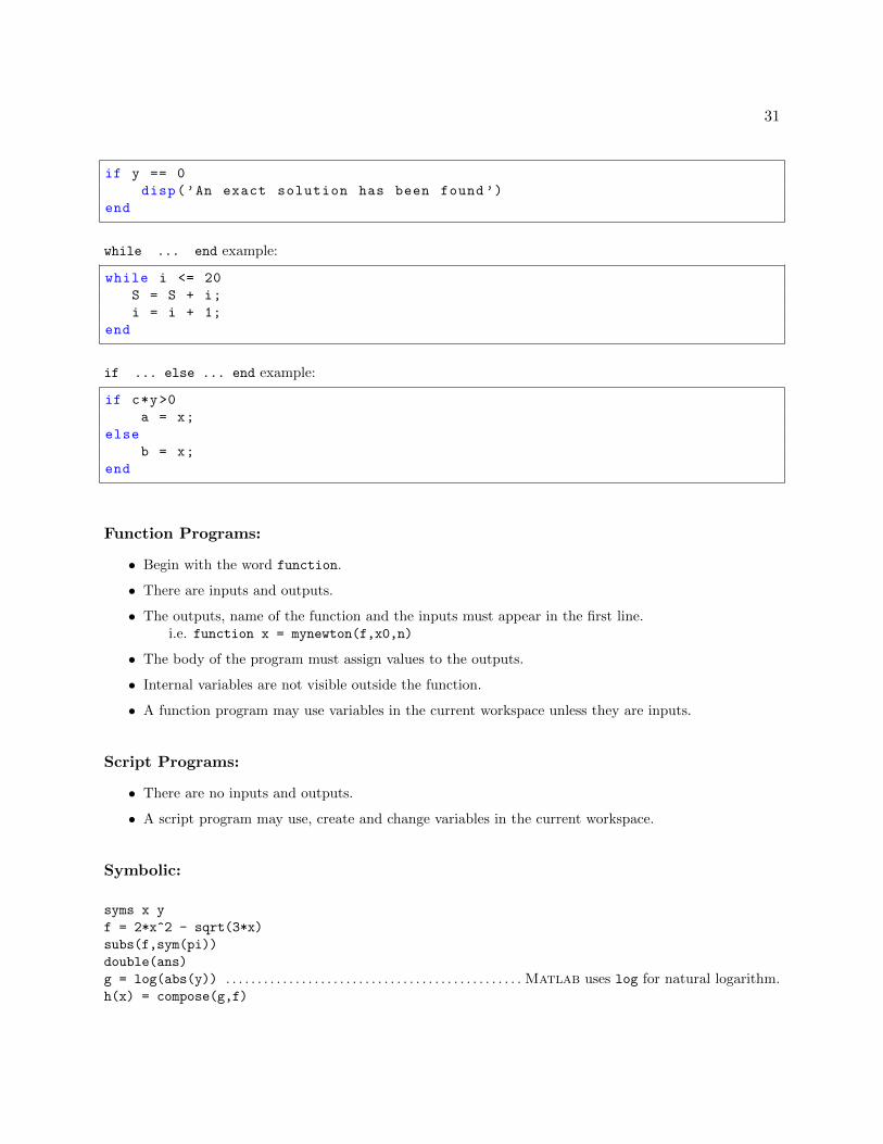
if ... end example:
31
if y == 0
disp(’An exact solution has been found’)
end
while ... end example:
while i <= 20
S = S + i;
i = i + 1;
end
if ... else ... end example:
if c*y>0
a = x;
else
b = x;
end
Function Programs:
• Begin with the word function.
• There are inputs and outputs.
• The outputs, name of the function and the inputs must appear in the first line.i.e. function x = mynewton(f,x0,n)
• The body of the program must assign values to the outputs.
• Internal variables are not visible outside the function.
• A function program may use variables in the current workspace unless they are inputs.
Script Programs:
• There are no inputs and outputs.
• A script program may use, create and change variables in the current workspace.
Symbolic:
syms x y
f = 2*x^2 - sqrt(3*x)
subs(f,sym(pi))
double(ans)
g = log(abs(y)) . . . . . . . . . . . . . . . . . . . . . . . . . . . . . . . . . . . . . . . . . . . . . . . Matlab uses log for natural logarithm.h(x) = compose(g,f)

32 REVIEW OF PART I
k(x,y) = f*g
ezplot(f)
ezplot(g,-10,10)
ezsurf(k)
f1 = diff(f,’x’)
F = int(f,’x’) . . . . . . . . . . . . . . . . . . . . . . . . . . . . . . . . . . . . . . . . . . . . . . . . . . . . . . . indefinite integral (antiderivative)int(f,0,2*pi) . . . . . . . . . . . . . . . . . . . . . . . . . . . . . . . . . . . . . . . . . . . . . . . . . . . . . . . . . . . . . . . . . . . . . . . . . . definite integralpoly = x*(x - 3)*(x-2)*(x-1)*(x+1)
polyex = expand(poly)
polysi = simple(polyex)
solve(f)
solve(g)
solve(polyex)

Part II
Linear Algebra
c©Copyright, Todd Young and Martin Mohlenkamp, Department of Mathematics, Ohio University, 2017
Lecture 8
Matrices and Matrix Operations in Matlab
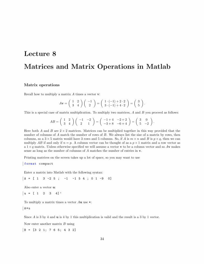
Matrix operations
Recall how to multiply a matrix A times a vector v:
Av =
(1 23 4
)(−12
)=
(1 · (−1) + 2 · 23 · (−1) + 4 · 2
)=
(35
).
This is a special case of matrix multiplication. To multiply two matrices, A and B you proceed as follows:
AB =
(1 23 4
)(−1 −22 1
)=
(−1 + 4 −2 + 2−3 + 8 −6 + 4
)=
(3 05 −2
).
Here both A and B are 2 × 2 matrices. Matrices can be multiplied together in this way provided that thenumber of columns of A match the number of rows of B. We always list the size of a matrix by rows, thencolumns, so a 3× 5 matrix would have 3 rows and 5 columns. So, if A is m× n and B is p× q, then we canmultiply AB if and only if n = p. A column vector can be thought of as a p× 1 matrix and a row vector asa 1× q matrix. Unless otherwise specified we will assume a vector v to be a column vector and so Av makessense as long as the number of columns of A matches the number of entries in v.
Printing matrices on the screen takes up a lot of space, so you may want to use
format compact
Enter a matrix into Matlab with the following syntax:
A = [ 1 3 -2 5 ; -1 -1 5 4 ; 0 1 -9 0]
Also enter a vector u:
u = [ 1 2 3 4]’
To multiply a matrix times a vector Au use *:
A*u
Since A is 3 by 4 and u is 4 by 1 this multiplication is valid and the result is a 3 by 1 vector.
Now enter another matrix B using
B = [3 2 1; 7 6 5; 4 3 2]
34
35
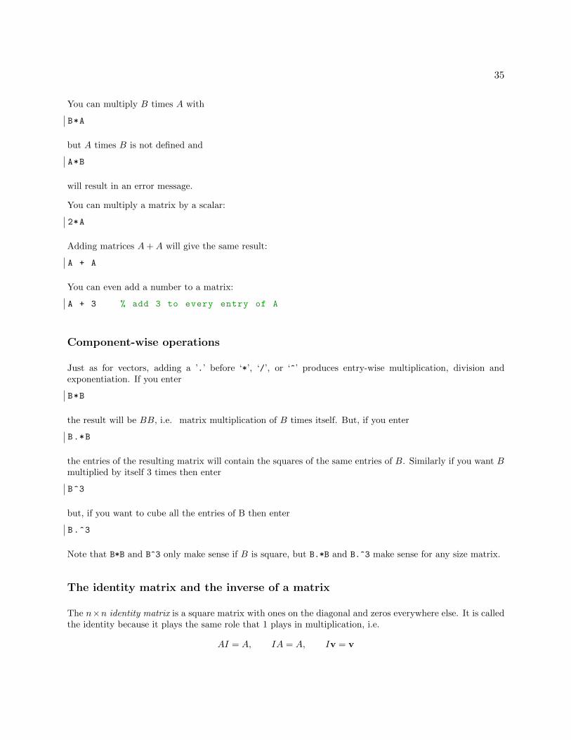
You can multiply B times A with
B*A
but A times B is not defined and
A*B
will result in an error message.
You can multiply a matrix by a scalar:
2*A
Adding matrices A+A will give the same result:
A + A
You can even add a number to a matrix:
A + 3 % add 3 to every entry of A
Component-wise operations
Just as for vectors, adding a ’.’ before ‘*’, ‘/’, or ‘^’ produces entry-wise multiplication, division andexponentiation. If you enter
B*B
the result will be BB, i.e. matrix multiplication of B times itself. But, if you enter
B.*B
the entries of the resulting matrix will contain the squares of the same entries of B. Similarly if you want Bmultiplied by itself 3 times then enter
B^3
but, if you want to cube all the entries of B then enter
B.^3
Note that B*B and B^3 only make sense if B is square, but B.*B and B.^3 make sense for any size matrix.
The identity matrix and the inverse of a matrix
The n×n identity matrix is a square matrix with ones on the diagonal and zeros everywhere else. It is calledthe identity because it plays the same role that 1 plays in multiplication, i.e.
AI = A, IA = A, Iv = v

36 LECTURE 8. MATRICES AND MATRIX OPERATIONS IN MATLAB
for any matrix A or vector v where the sizes match. An identity matrix in Matlab is produced by thecommand
I = eye(3)
A square matrix A can have an inverse which is denoted by A−1. The definition of the inverse is that
AA−1 = I and A−1A = I.
In theory an inverse is very important, because if you have an equation
Ax = b
where A and b are known and x is unknown (as we will see, such problems are very common and important)then the theoretical solution is
x = A−1b.
We will see later that this is not a practical way to solve an equation, and A−1 is only important for thepurpose of derivations. In Matlab we can calculate a matrix’s inverse very conveniently:
C = randn (5,5)
inv(C)
However, not all square matrices have inverses:
D = ones (5,5)
inv(D)
The “Norm” of a matrix
For a vector, the “norm” means the same thing as the length (geometrically, not the number of entries).Another way to think of it is how far the vector is from being the zero vector. We want to measure a matrixin much the same way and the norm is such a quantity. The usual definition of the norm of a matrix is
Definition 1 Suppose A is a m× n matrix. The norm of A is
‖A‖ ≡ max‖v‖=1
‖Av‖.
The maximum in the definition is taken over all vectors with length 1 (unit vectors), so the definition meansthe largest factor that the matrix stretches (or shrinks) a unit vector. This definition seems cumbersome atfirst, but it turns out to be the best one. For example, with this definition we have the following inequalityfor any vector v:
‖Av‖ ≤ ‖A‖‖v‖.
In Matlab the norm of a matrix is obtained by the command
norm(A)
For instance the norm of an identity matrix is 1:
37
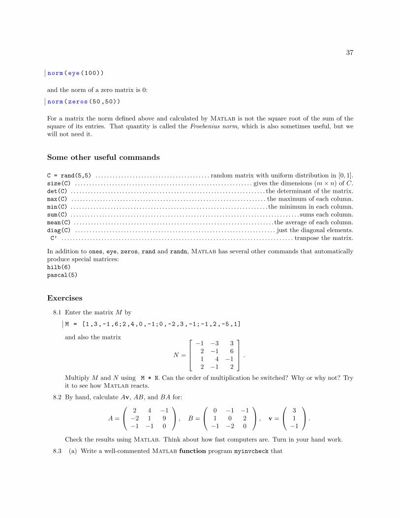
norm(eye (100))
and the norm of a zero matrix is 0:
norm(zeros (50 ,50))
For a matrix the norm defined above and calculated by Matlab is not the square root of the sum of thesquare of its entries. That quantity is called the Froebenius norm, which is also sometimes useful, but wewill not need it.
Some other useful commands
C = rand(5,5) . . . . . . . . . . . . . . . . . . . . . . . . . . . . . . . . . . . . . . . . random matrix with uniform distribution in [0, 1].size(C) . . . . . . . . . . . . . . . . . . . . . . . . . . . . . . . . . . . . . . . . . . . . . . . . . . . . . . . . . . . . . . gives the dimensions (m× n) of C.det(C) . . . . . . . . . . . . . . . . . . . . . . . . . . . . . . . . . . . . . . . . . . . . . . . . . . . . . . . . . . . . . . . . . . . . the determinant of the matrix.max(C) . . . . . . . . . . . . . . . . . . . . . . . . . . . . . . . . . . . . . . . . . . . . . . . . . . . . . . . . . . . . . . . . . . . . the maximum of each column.min(C) . . . . . . . . . . . . . . . . . . . . . . . . . . . . . . . . . . . . . . . . . . . . . . . . . . . . . . . . . . . . . . . . . . . . . the minimum in each column.sum(C) . . . . . . . . . . . . . . . . . . . . . . . . . . . . . . . . . . . . . . . . . . . . . . . . . . . . . . . . . . . . . . . . . . . . . . . . . . . . . . . . sums each column.mean(C) . . . . . . . . . . . . . . . . . . . . . . . . . . . . . . . . . . . . . . . . . . . . . . . . . . . . . . . . . . . . . . . . . . . . . .the average of each column.diag(C) . . . . . . . . . . . . . . . . . . . . . . . . . . . . . . . . . . . . . . . . . . . . . . . . . . . . . . . . . . . . . . . . . . . . . . just the diagonal elements.C’ . . . . . . . . . . . . . . . . . . . . . . . . . . . . . . . . . . . . . . . . . . . . . . . . . . . . . . . . . . . . . . . . . . . . . . . . . . . . . . . . . tranpose the matrix.
In addition to ones, eye, zeros, rand and randn, Matlab has several other commands that automaticallyproduce special matrices:hilb(6)
pascal(5)
Exercises
8.1 Enter the matrix M by
M = [1,3,-1,6;2,4,0,-1;0,-2,3,-1;-1,2,-5,1]
and also the matrix
N =
−1 −3 3
2 −1 61 4 −12 −1 2
.Multiply M and N using M * N. Can the order of multiplication be switched? Why or why not? Tryit to see how Matlab reacts.
8.2 By hand, calculate Av, AB, and BA for:
A =
2 4 −1−2 1 9−1 −1 0
, B =
0 −1 −11 0 2−1 −2 0
, v =
31−1
.
Check the results using Matlab. Think about how fast computers are. Turn in your hand work.
8.3 (a) Write a well-commented Matlab function program myinvcheck that

38 LECTURE 8. MATRICES AND MATRIX OPERATIONS IN MATLAB
• makes a n× n random matrix (normally distributed, A = randn(n,n)),
• calculates its inverse (B = inv(A)),
• multiplies the two back together,
• calculates the residual (difference from the desired n× n identity matrix eye(n)), and
• returns the norm of the residual.
(b) Write a well-commented Matlab script program that calls myinvcheck for n = 10, 20, 40, . . . , 2i10for some moderate i, records the results of each trial, and plots the error versus n using a logplot. (See help loglog.)
What happens to error as n gets big? Turn in a printout of the programs, the plot, and a very briefreport on the results of your experiments.
Lecture 9
Introduction to Linear Systems
How linear systems occur
Linear systems of equations naturally occur in many places in engineering, such as structural analysis,dynamics and electric circuits. Computers have made it possible to quickly and accurately solve largerand larger systems of equations. Not only has this allowed engineers to handle more and more complexproblems where linear systems naturally occur, but has also prompted engineers to use linear systems tosolve problems where they do not naturally occur such as thermodynamics, internal stress-strain analysis,fluids and chemical processes. It has become standard practice in many areas to analyze a problem bytransforming it into a linear systems of equations and then solving those equation by computer. In this way,computers have made linear systems of equations the most frequently used tool in modern engineering.
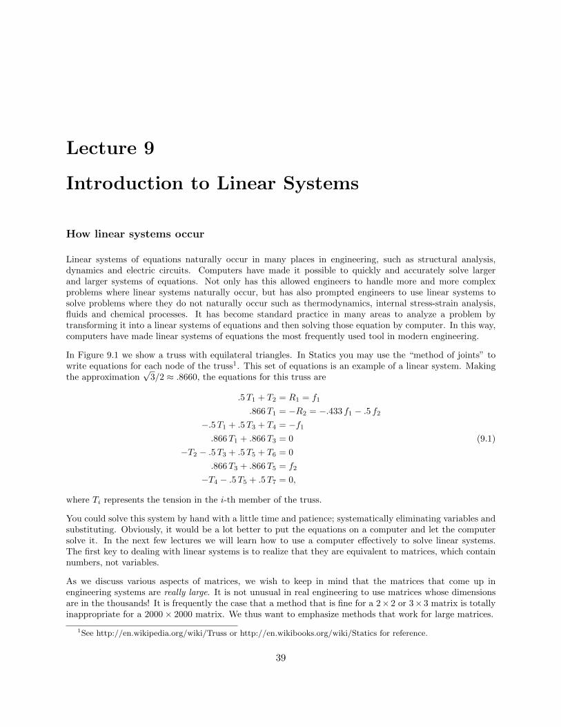
In Figure 9.1 we show a truss with equilateral triangles. In Statics you may use the “method of joints” towrite equations for each node of the truss1. This set of equations is an example of a linear system. Makingthe approximation
√3/2 ≈ .8660, the equations for this truss are
.5T1 + T2 = R1 = f1
.866T1 = −R2 = −.433 f1 − .5 f2−.5T1 + .5T3 + T4 = −f1.866T1 + .866T3 = 0
−T2 − .5T3 + .5T5 + T6 = 0
.866T3 + .866T5 = f2
−T4 − .5T5 + .5T7 = 0,
(9.1)
where Ti represents the tension in the i-th member of the truss.
You could solve this system by hand with a little time and patience; systematically eliminating variables andsubstituting. Obviously, it would be a lot better to put the equations on a computer and let the computersolve it. In the next few lectures we will learn how to use a computer effectively to solve linear systems.The first key to dealing with linear systems is to realize that they are equivalent to matrices, which containnumbers, not variables.
As we discuss various aspects of matrices, we wish to keep in mind that the matrices that come up inengineering systems are really large. It is not unusual in real engineering to use matrices whose dimensionsare in the thousands! It is frequently the case that a method that is fine for a 2× 2 or 3× 3 matrix is totallyinappropriate for a 2000× 2000 matrix. We thus want to emphasize methods that work for large matrices.
1See http://en.wikipedia.org/wiki/Truss or http://en.wikibooks.org/wiki/Statics for reference.
39

40 LECTURE 9. INTRODUCTION TO LINEAR SYSTEMS
u r u
r r
A
B
C
D
E
1
2
3
4
5
6
7
-f1
?f2
6
R2
6
R3
R1
Figure 9.1: An equilateral truss. Joints or nodes are labeled alphabetically, A, B, . . . and Members(edges) are labeled numerically: 1, 2, . . . . The forces f1 and f2 are applied loads and R1, R2 andR3 are reaction forces applied by the supports.
Linear systems are equivalent to matrix equations
The system of linear equations
x1 − 2x2 + 3x3 = 4
2x1 − 5x2 + 12x3 = 15
2x2 − 10x3 = −10
is equivalent to the matrix equation 1 −2 32 −5 120 2 −10
x1x2x3
=
415−10
,
which is equivalent to the augmented matrix 1 −2 3 42 −5 12 150 2 −10 −10
.
The advantage of the augmented matrix, is that it contains only numbers, not variables. The reason this isbetter is because computers are much better in dealing with numbers than variables. To solve this system,the main steps are called Gaussian elimination and back substitution.
The augmented matrix for the equilateral truss equations (9.1) is given by
.5 1 0 0 0 0 0 f1.866 0 0 0 0 0 0 −.433f1 − .5 f2−.5 0 .5 1 0 0 0 −f1.866 0 .866 0 0 0 0 0
0 −1 −.5 0 .5 1 0 00 0 .866 0 .866 0 0 f20 0 0 −1 −.5 0 .5 0
. (9.2)
Notice that a lot of the entries are 0. Matrices like this, called sparse, are common in applications and thereare methods specifically designed to efficiently handle sparse matrices.

41
Triangular matrices and back substitution
Consider a linear system whose augmented matrix happens to be 1 −2 3 40 −1 6 70 0 2 4
. (9.3)
Recall that each row represents an equation and each column a variable. The last row represents the equation2x3 = 4. The equation is easily solved, i.e. x3 = 2. The second row represents the equation −x2 + 6x3 = 7,but since we know x3 = 2, this simplifies to: −x2 + 12 = 7. This is easily solved, giving x2 = 5. Finally,since we know x2 and x3, the first row simplifies to: x1 − 10 + 6 = 4. Thus we have x1 = 8 and so we knowthe whole solution vector: x = 〈8, 5, 2〉. The process we just did is called back substitution, which is bothefficient and easily programmed. The property that made it possible to solve the system so easily is thatA in this case is upper triangular. In the next section we show an efficient way to transform an augmentedmatrix into an upper triangular matrix.
Gaussian Elimination
Consider the matrix
A =
1 −2 3 42 −5 12 150 2 −10 −10
.
The first step of Gaussian elimination is to get rid of the 2 in the (2,1) position by subtracting 2 times thefirst row from the second row, i.e. (new 2nd = old 2nd - (2) 1st). We can do this because it is essentially thesame as adding equations, which is a valid algebraic operation. This leads to 1 −2 3 4
0 −1 6 70 2 −10 −10
.
There is already a zero in the lower left corner, so we don’t need to eliminate anything there. To eliminatethe third row, second column, we need to subtract −2 times the second row from the third row, (new 3rd =old 3rd - (-2) 2nd), to obtain 1 −2 3 4
0 −1 6 70 0 2 4
.
This is now just exactly the matrix in equation (9.3), which we can now solve by back substitution.
Matlab’s matrix solve command
In Matlab the standard way to solve a system Ax = b is by the command
x = A \ b
This command carries out Gaussian elimination and back substitution. We can do the above computationsas follows:
42 LECTURE 9. INTRODUCTION TO LINEAR SYSTEMS
A = [1 -2 3 ; 2 -5 12 ; 0 2 -10]
b = [4 15 -10]’
x = A \ b
Next, use the Matlab commands above to solve Ax = b when the augmented matrix for the system is 1 2 3 45 6 7 89 10 11 12
,
by entering
x1 = A \ b
Check the result by entering
A*x1 - b
You will see that the resulting answer satisfies the equation exactly. Next try solving using the inverse of A:
x2 = inv(A)*b
This answer can be seen to be inaccurate by checking
A*x2 - b
Thus we see one of the reasons why the inverse is never used for actual computations, only for theory.
Exercises
9.1 Set f1 = 1000N and f2 = 5000N in the equations (9.1) for the equailateral truss. Input the coefficientmatrix A and the right hand side vector b in (9.2) into Matlab. Solve the system using the command\ to find the tension in each member of the truss. Save the matrix A as A_equil_truss and keep itfor later use. (Enter save A_equil_truss A.) Print out and turn in A, b and the solution x.
9.2 Write each system of equations as an augmented matrix, then find the solutions using Gaussianelimination and back substitution (the algorithm in this chapter). Check your solutions using Matlab.
(a)
x1 + x2 = 2
4x1 + 5x2 = 10
(b)
x1 + 2x2 + 3x3 = −1
4x1 + 7x2 + 14x3 = 3
x1 + 4x2 + 4x3 = 1
Lecture 10
Some Facts About Linear Systems
Some inconvenient truths
In the last lecture we learned how to solve a linear system using Matlab. Input the following:
A = ones (4,4)
b = randn (4,1)
x = A \ b
As you will find, there is no solution to the equation Ax = b. This unfortunate circumstance is mostly thefault of the matrix, A, which is too simple, its columns (and rows) are all the same. Now try
b = ones (4,1)
x = [ 1 0 0 0]’
A*x
So the system Ax = b does have a solution. Still unfortunately, that is not the only solution. Try
x = [ 0 1 0 0]’
A*x
We see that this x is also a solution. Next try
x = [ -4 5 2.27 -2.27]’
A*x
This x is a solution! It is not hard to see that there are endless possibilities for solutions of this equation.
Basic theory
The most basic theoretical fact about linear systems is
Theorem 1 A linear system Ax = b may have 0, 1, or infinitely many solutions.
Obviously, in most engineering applications we would want to have exactly one solution. The following twotheorems tell us exactly when we can and cannot expect this.
43

44 LECTURE 10. SOME FACTS ABOUT LINEAR SYSTEMS
Theorem 2 Suppose A is a square (n× n) matrix. The following are all equivalent:
1. The equation Ax = b has exactly one solution for any b.
2. det(A) 6= 0.
3. A has an inverse.
4. The only solution of Ax = 0 is x = 0.
5. The columns of A are linearly independent (as vectors).
6. The rows of A are linearly independent.
If A has these properties then it is called non-singular.
On the other hand, a matrix that does not have these properties is called singular.
Theorem 3 Suppose A is a square matrix. The following are all equivalent:
1. The equation Ax = b has 0 or ∞ many solutions depending on b.
2. det(A) = 0.
3. A does not have an inverse.
4. The equation Ax = 0 has solutions other than x = 0.
5. The columns of A are linearly dependent as vectors.
6. The rows of A are linearly dependent.
To see how the two theorems work, define two matrices (type in A1 then scroll up and modify to make A2) :
A1 =
1 2 34 5 67 8 9
, A2 =
1 2 34 5 67 8 8
,
and two vectors:
b1 =
036
, b2 =
136
.
First calculate the determinants of the matrices:
det(A1)
det(A2)
Then attempt to find the inverses:
inv(A1)
inv(A2)
Which matrix is singular and which is non-singular? Finally, attempt to solve all the possible equationsAx = b:

45
x = A1 \ b1
x = A1 \ b2
x = A2 \ b1
x = A2 \ b2
As you can see, equations involving the non-singular matrix have one and only one solution, but equationinvolving a singular matrix are more complicated.
The Residual
Recall that the residual for an approximate solution x of an equation f(x) = 0 is defined as r = ‖f(x)‖. Itis a measure of how close the equation is to being satisfied. For a linear system of equations we define theresidual vector of an approximate solution x by
r = Ax− b.
If the solution vector x were exactly correct, then r would be exactly the zero vector. The size (norm) of ris an indication of how close we have come to solving Ax = b. We will refer to this number as the scalarresidual or just Residual of the approximation solution:
r = ‖Ax− b‖. (10.1)
Exercises
10.1 By hand, find all the solutions (if any) of the following linear system using the augmented matrix andGaussian elimination:
x1 + 2x2 + 3x3 = 4,
4x1 + 5x2 + 6x3 = 10,
7x1 + 8x2 + 9x3 = 14 .
10.2 (a) Write a well-commented Matlab function program mysolvecheck with input a number n thatmakes a random n × n matrix A and a random vector b, solves the linear system Ax = b,calculates the scalar residual r = ‖Ax− b‖, and outputs that number as r.
(b) Write a well-commented Matlab script program that calls mysolvecheck 10 times each forn = 10, 50, 100, 500, and 1000, records and averages the results and makes a log-log plot of theaverage e vs. n. Increase the maximum n until the program stops running within 5 minutes.
Turn in the plot and the two programs.

Lecture 11
Accuracy, Condition Numbers and Pivoting
In this lecture we will discuss two separate issues of accuracy in solving linear systems. The first, pivoting, isa method that ensures that Gaussian elimination proceeds as accurately as possible. The second, conditionnumber, is a measure of how bad a matrix is. We will see that if a matrix has a bad condition number, thesolutions are unstable with respect to small changes in data.
The effect of rounding
All computers store numbers as finite strings of binary floating point digits (bits). This limits numbers toa fixed number of significant digits and implies that after even the most basic calculations, rounding musthappen.
Consider the following exaggerated example. Suppose that our computer can only store 2 significant digitsand it is asked to do Gaussian elimination on(
.001 1 31 2 5
).
Doing the elimination exactly would produce(.001 1 3
0 −998 −2995
),
but rounding to 2 digits, our computer would store this as(.001 1 3
0 −1000 −3000
).
Backsolving this reduced system givesx1 = 0 and x2 = 3.
This seems fine until you realize that backsolving the unrounded system gives
x1 = −1 and x2 = 3.001.
Row Pivoting
A way to fix the problem is to use pivoting, which means to switch rows of the matrix. Since switching rowsof the augmented matrix just corresponds to switching the order of the equations, no harm is done:(
1 2 5.001 1 3
).
46

47
Exact elimination would produce (1 2 50 .998 2.995
).
Storing this result with only 2 significant digits gives(1 2 50 1 3
).
Now backsolving producesx1 = −1 and x2 = 3,
which is the true solution (rounded to 2 significant digits).
The reason this worked is because 1 is bigger than 0.001. To pivot we switch rows so that the largest entryin a column is the one used to eliminate the others. In bigger matrices, after each column is completed,compare the diagonal element of the next column with all the entries below it. Switch it (and the entire row)with the one with greatest absolute value. For example in the following matrix, the first column is finishedand before doing the second column, pivoting should occur since | − 2| > |1|: 1 −2 3 4
0 1 6 70 −2 −10 −10
.
Pivoting the 2nd and 3rd rows would produce 1 −2 3 40 −2 −10 −100 1 6 7
.
Condition number
In some systems, problems occur even without rounding. Consider the following augmented matrices:(1 1/2 3/2
1/2 1/3 1
)and
(1 1/2 3/2
1/2 1/3 5/6
).
Here we have the same A, but two different input vectors:
b1 = (3/2, 1)′ and b2 = (3/2, 5/6)′
which are pretty close to one another. You would expect then that the solutions x1 and x2 would also beclose. Notice that this matrix does not need pivoting. Eliminating exactly we get(
1 1/2 3/20 1/12 1/4
)and
(1 1/2 3/20 1/12 1/12
).
Now solving we findx1 = (0, 3)′ and x2 = (1, 1)′
which are not close at all despite the fact that we did the calculations exactly. This poses a new problem:some matrices are very sensitive to small changes in input data. The extent of this sensitivity is measured
48 LECTURE 11. ACCURACY, CONDITION NUMBERS AND PIVOTING
by the condition number. The definition of condition number is: consider all small changes δA and δb inA and b and the resulting change, δx, in the solution x. Then
cond(A) ≡ max
‖δx‖/‖x‖‖δA‖‖A‖ + ‖δb‖
‖b‖
= max
(Relative error of output
Relative error of inputs
).
Put another way, changes in the input data get multiplied by the condition number to produce changes inthe outputs. Thus a high condition number is bad. It implies that small errors in the input can cause largeerrors in the output.
In Matlab enter
H = hilb (2)
which should result in the matrix above. Matlab produces the condition number of a matrix with thecommand
cond(H)
Thus for this matrix small errors in the input can get magnified by 19 in the output. Next try the matrix
A = [ 1.2969 0.8648 ; .2161 .1441]
cond(A)
For this matrix small errors in the input can get magnified by 2.5 × 10⁸ in the output! (We will see thishappen in the exercise.) This is obviously not very good for engineering where all measurements, constantsand inputs are approximate.
Is there a solution to the problem of bad condition numbers? Usually, bad condition numbers in engineeringcontexts result from poor design. So, the engineering solution to bad conditioning is redesign.
Finally, find the determinant of the matrix A above:
det(A)
which will be small. If det(A) = 0 then the matrix is singular, which is bad because it implies therewill not be a unique solution. The case here, det(A) ≈ 0, is also bad, because it means the matrix isalmost singular. Although det(A) ≈ 0 generally indicates that the condition number will be large, theyare actually independent things. To see this, find the determinant and condition number of the matrix[1e-10,0;0,1e-10] and the matrix [1e+10,0;0,1e-10].

49
Exercises
11.1 Let
A =
[1.2969 .8648.2161 .1441
].
(a) Find the determinant and inverse of A (using Matlab).
(b) Let B be the matrix obtained from A by rounding off to three decimal places (1.2969 7→ 1.297).Find the determinant and inverse of B. How do A−1 and B−1 differ? Explain how this happened.
(c) Set b1 = [1.2969; 0.2161] and do x = A \ b1 . Repeat the process but with a vector b2
obtained from b1 by rounding off to three decimal places. Explain exactly what happened. Whywas the first answer so simple? Why do the two answers differ by so much?
11.2 Try
B = [sin(sym (1)) sin(sym (2)); sin(sym (3)) sin(sym (4))]
c = [1; 2]
x = B \ c
pretty(x)
Next input the matrix:
Cs =
[1 22 4
]symbolically as above by wrapping each number in sym. Create a numerical version via Cn = double(Cs)
and define the two vectors d1 = [4; 8] and d2 = [1; 1]. Solve the systems Cs*x = d1, Cn*x = d1,Cs*x = d2, and Cn*x = d2. Explain the results. Does the symbolic or non-symbolic way give moreinformation?
11.3 Recall the matrixA that you saved using A_equil_truss in exercise 9.1. (Enter > load A_equil_truss
or click on the file A_equil_truss.mat in the folder where you saved it; this should reproduce thematrix A.)
Find the condition number for this matrix. Write a well-commented script program to calculatethe mean and median condition number of 1000 randomly generated 7 by 7 matrices. How does thecondition number of the truss matrix compare to randomly generated matrices? Turn in your scriptwith the answers to these questions.

Lecture 12
LU Decomposition
In many applications where linear systems appear, one needs to solve Ax = b for many different vectors b.For instance, a structure must be tested under several different loads, not just one. As in the example of atruss (9.2), the loading in such a problem is usually represented by the vector b. Gaussian elimination withpivoting is the most efficient and accurate way to solve a linear system. Most of the work in this method isspent on the matrix A itself. If we need to solve several different systems with the same A, and A is big,then we would like to avoid repeating the steps of Gaussian elimination on A for every different b. This canbe accomplished by the LU decomposition, which in effect records the steps of Gaussian elimination.
LU decomposition
The main idea of the LU decomposition is to record the steps used in Gaussian elimination on A in theplaces where the zero is produced. Consider the matrix
A =
1 −2 32 −5 120 2 −10
.
The first step of Gaussian elimination is to subtract 2 times the first row from the second row. In order torecord what we have done, we will put the multiplier, 2, into the place it was used to make a zero, i.e. thesecond row, first column. In order to make it clear that it is a record of the step and not an element of A,we will put it in parentheses. This leads to 1 −2 3
(2) −1 60 2 −10
.
There is already a zero in the lower left corner, so we don’t need to eliminate anything there. We record thisfact with a (0). To eliminate the third row, second column, we need to subtract −2 times the second rowfrom the third row. Recording the −2 in the spot it was used we have 1 −2 3
(2) −1 6(0) (−2) 2
.
Let U be the upper triangular matrix produced, and let L be the lower triangular matrix with the recordsand ones on the diagonal, i.e.
L =
1 0 02 1 00 −2 1
and U =
1 −2 30 −1 60 0 2
,
50
51
then we have the following wonderful property:
LU =
1 0 02 1 00 −2 1
1 −2 30 −1 60 0 2
=
1 −2 32 −5 120 2 −10
= A.
Thus we see that A is actually the product of L and U . Here L is lower triangular and U is upper triangular.When a matrix can be written as a product of simpler matrices, we call that a decomposition of A and thisone we call the LU decomposition.
Using LU to solve equations
If we also include pivoting, then an LU decomposition for A consists of three matrices P , L and U such that
PA = LU. (12.1)
The pivot matrix P is the identity matrix, with the same rows switched as the rows of A are switched in thepivoting. For instance,
P =
1 0 00 0 10 1 0
,
would be the pivot matrix if the second and third rows of A are switched by pivoting. Matlab will producean LU decomposition with pivoting for a matrix A with the command> [L U P] = lu(A)
where P is the pivot matrix. To use this information to solve Ax = b we first pivot both sides by multiplyingby the pivot matrix:
PAx = Pb ≡ d.
Substituting LU for PA we get
LUx = d.
Then we define y = Ux, which is unknown since x is unknown. Using forward-substitution, we can (easily)solve
Ly = d
for y and then using back-substitution we can (easily) solve
Ux = y
for x. In Matlab this would work as follows:
A = rand (5,5)
[L U P] = lu(A)
b = rand (5,1)
d = P*b
y = L\d
x = U\y
rnorm = norm(A*x - b) % Check the result
52 LECTURE 12. LU DECOMPOSITION
We can then solve for any other b without redoing the LU step. Repeat the sequence for a new right handside: c = randn(5,1); you can start at the third line. While this may not seem like a big savings, it wouldbe if A were a large matrix from an actual application.
The LU decomposition is an example of Matrix Decomposition which means taking a general matrix A andbreaking it down into components with simpler properties. Here L and U are simpler because they are lowerand upper triangular. There are many other matrix decompositions that are useful in various contexts.Some of the most useful of these are the QR decomposition, the Singular Value decomposition and Choleskydecomposition.
Exercises
12.1 Solve the systems below by hand using Gaussian elimination and back substitution on the augmentedmatrix. As a by-product, find the LU decomposition of A. Pivot wherever appropriate. Check byhand that LU = PA and Ax = b.
(a) A =
(2 4.5 4
), b =
(0−3
)(b) A =
(1 43 5
), b =
(32
)12.2 Finish the following Matlab function program:
function [x1, r1, x2, r2] = mysolve(A,b)
% Solves linear systems using the LU decomposition with pivoting
% and also with the built -in solve function A\b.
% Inputs: A -- the matrix
% b -- the right -hand vector
% Outputs: x1 -- the solution using the LU method
% r1 -- the norm of the residual using the LU method
% x2 -- the solution using the built -in method
% r2 -- the norm of the residual using the
% built -in method
Using format long, test the program on both random matrices (randn(n,n)) and Hilbert matrices(hilb(n)) with n large (as big as you can make it and the program still run). Print your programand summarize your observations. (Do not print any random matrices or vectors.)
Lecture 13
Nonlinear Systems - Newton’s Method
An Example
The LORAN (LOng RAnge Navigation) system calculates the position of a boat at sea using signals fromfixed transmitters. From the time differences of the incoming signals, the boat obtains differences of distancesto the transmitters. This leads to two equations each representing hyperbolas defined by the differences ofdistance of two points (foci). An example of such equations1 are
x2
1862− y2
3002 − 1862= 1 and
(y − 500)2
2792− (x− 300)2
5002 − 2792= 1 .
(13.1)
Solving two quadratic equations with two unknowns, would require solving a 4 degree polynomial equation.We could do this by hand, but for a navigational system to work well, it must do the calculations automat-ically and numerically. We note that the Global Positioning System (GPS) works on similar principles andmust do similar computations.
Vector Notation
In general, we can usually find solutions to a system of equations when the number of unknowns matchesthe number of equations. Thus, we wish to find solutions to systems that have the form
f1(x1, x2, x3, . . . , xn) = 0
f2(x1, x2, x3, . . . , xn) = 0
f3(x1, x2, x3, . . . , xn) = 0
...
fn(x1, x2, x3, . . . , xn) = 0.
(13.2)
For convenience we can think of (x1, x2, x3, . . . , xn) as a vector x and (f1, f2, . . . , fn) as a vector-valuedfunction f . With this notation, we can write the system of equations (13.2) simply as
f(x) = 0,
1E. Johnston, J. Mathews, Calculus, Addison-Wesley, 2001
53

54 LECTURE 13. NONLINEAR SYSTEMS - NEWTON’S METHOD
i.e. we wish to find a vector that makes the vector function equal to the zero vector.
As in Newton’s method for one variable, we need to start with an initial guess x0. In theory, the morevariables one has, the harder it is to find a good initial guess. In practice, this must be overcome by usingphysically reasonable assumptions about the possible values of a solution, i.e. take advantage of engineeringknowledge of the problem. Once x0 is chosen, let
∆x = x1 − x0.
Linear Approximation for Vector Functions
In the single variable case, Newton’s method was derived by considering the linear approximation of thefunction f at the initial guess x0. From Calculus, the following is the linear approximation of f at x0, forvectors and vector-valued functions:
f(x) ≈ f(x0) +Df(x0)(x− x0).
Here Df(x0) is an n × n matrix whose entries are the various partial derivative of the components of f ,evaluated at x0. Specifically,
Df(x0) =
∂f1∂x1
(x0) ∂f1∂x2
(x0) ∂f1∂x3
(x0) . . . ∂f1∂xn
(x0)
∂f2∂x1
(x0) ∂f2∂x2
(x0) ∂f2∂x3
(x0) . . . ∂f2∂xn
(x0)
......
.... . .
...
∂fn∂x1
(x0) ∂fn∂x2
(x0) ∂fn∂x3
(x0) . . . ∂fn∂xn
(x0)
. (13.3)
Newton’s Method
We wish to find x that makes f equal to the zero vectors, so let’s choose x1 so that
f(x0) +Df(x0)(x1 − x0) = 0.
Since Df(x0) is a square matrix, we can solve this equation by
x1 = x0 − (Df(x0))−1f(x0),
provided that the inverse exists. The formula is the vector equivalent of the Newton’s method formula welearned before. However, in practice we never use the inverse of a matrix for computations, so we cannotuse this formula directly. Rather, we can do the following. First solve the equation
Df(x0)∆x = −f(x0). (13.4)
Since Df(x0) is a known matrix and −f(x0) is a known vector, this equation is just a system of linearequations, which can be solved efficiently and accurately. Once we have the solution vector ∆x, we canobtain our improved estimate x1 by
x1 = x0 + ∆x.
For subsequent steps, we have the following process:
• Solve Df(xi)∆x = −f(xi) for ∆x.
• Let xi+1 = xi + ∆x
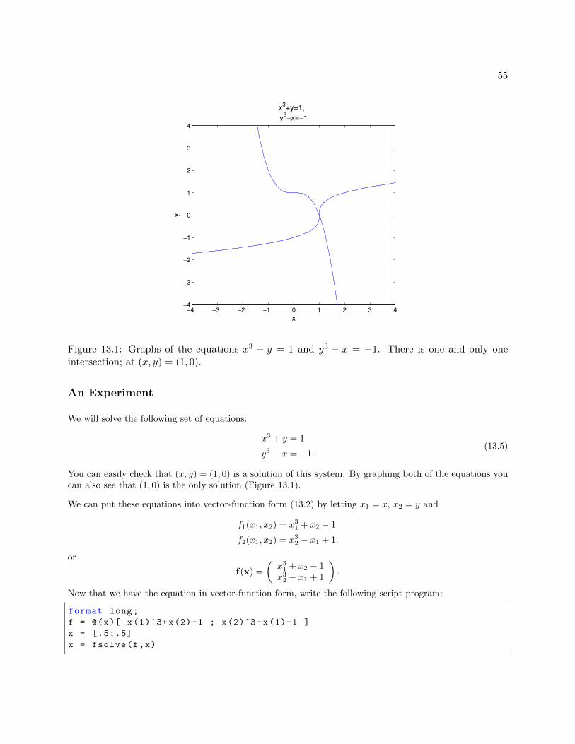
55
−4 −3 −2 −1 0 1 2 3 4−4
−3
−2
−1
0
1
2
3
4
x
y
x3+y=1,
y3−x=−1
Figure 13.1: Graphs of the equations x3 + y = 1 and y3 − x = −1. There is one and only oneintersection; at (x, y) = (1, 0).
An Experiment
We will solve the following set of equations:
x3 + y = 1
y3 − x = −1.(13.5)
You can easily check that (x, y) = (1, 0) is a solution of this system. By graphing both of the equations youcan also see that (1, 0) is the only solution (Figure 13.1).
We can put these equations into vector-function form (13.2) by letting x1 = x, x2 = y and
f1(x1, x2) = x31 + x2 − 1
f2(x1, x2) = x32 − x1 + 1.
or
f(x) =
(x31 + x2 − 1x32 − x1 + 1
).
Now that we have the equation in vector-function form, write the following script program:
format long;
f = @(x)[ x(1)^3+x(2)-1 ; x(2)^3 -x(1)+1 ]
x = [.5;.5]
x = fsolve(f,x)
56 LECTURE 13. NONLINEAR SYSTEMS - NEWTON’S METHOD
Save this program as myfsolve.m and run it. You will see that the internal Matlab solving commandfsolve approximates the solution, but only to about 7 decimal places. While that would be close enoughfor most applications, one would expect that we could do better on such a simple problem.
Next we will implement Newton’s method for this problem. Modify your myfsolve program to:
% mymultnewton
format long;
n=8 % set some number of iterations , may need adjusting
f = @(x)[x(1)^3+x(2)-1 ; x(2)^3 -x(1)+1] % the vector function
% the matrix of partial derivatives
Df = @(x)[3*x(1)^2, 1 ; -1, 3*x(2)^2]
x = [.5;.5] % starting guess
for i = 1:n
Dx = -Df(x)\f(x); % solve for increment
x = x + Dx % add on to get new guess
f(x) % see if f(x) is really zero
end
Save and run this program (as mymultnewton) and you will see that it finds the root exactly (to machineprecision) in only 6 iterations. Why is this simple program able to do better than Matlab’s built-in program?
Exercises
13.1 (a) Put the LORAN equations (13.1) into the function form (13.2).
(b) Construct the matrix of partial derivatives Df in (13.3).
(c) Adapt the mymultnewton program to find a solution for these equations. By trying differentstarting vectors, find at least three different solutions. (There are actually four solutions.) Thinkof at least one way that the navigational system could determine which solution is correct.
Lecture 14
Eigenvalues and Eigenvectors
Suppose that A is a square (n× n) matrix. We say that a nonzero vector v is an eigenvector and a numberλ is its eigenvalue if
Av = λv. (14.1)
Geometrically this means that Av is in the same direction as v, since multiplying a vector by a numberchanges its length, but not its direction.
Matlab has a built-in routine for finding eigenvalues and eigenvectors:
A = pascal (4)
[v e] = eig(A)
The results are a matrix v that contains eigenvectors as columns and a diagonal matrix e that containseigenvalues on the diagonal. We can check this by
v1 = v(:,1)
A*v1
e(1 ,1)*v1
Finding Eigenvalues for 2× 2 and 3× 3
If A is 2× 2 or 3× 3 then we can find its eigenvalues and eigenvectors by hand. Notice that Equation (14.1)can be rewritten as
Av − λv = 0.
It would be nice to factor out the v from the right-hand side of this equation, but we can’t because A is amatrix and λ is a number. However, since Iv = v, we can do the following:
Av − λv = Av − λIv= (A− λI)v
= 0
If v is nonzero, then by Theorem 3 in Lecture 10 the matrix (A−λI) must be singular. By the same theorem,we must have
det(A− λI) = 0.
This is called the characteristic equation.
57

58 LECTURE 14. EIGENVALUES AND EIGENVECTORS
For a 2× 2 matrix, A− λI is calculated as in the following example:
A− λI =
(1 43 5
)− λ
(1 00 1
)=
(1 43 5
)−(λ 00 λ
)=
(1− λ 4
3 5− λ
).
The determinant of A− λI is then
det(A− λI) = (1− λ)(5− λ)− 4 · 3= −7− 6λ+ λ2.
The characteristic equation det(A− λI) = 0 is simply a quadratic equation:
λ2 − 6λ− 7 = 0.
The roots of this equation are λ1 = 7 and λ2 = −1. These are the eigenvalues of the matrix A. Now to findthe corresponding eigenvectors we return to the equation (A − λI)v = 0. For λ1 = 7, the equation for theeigenvector (A− λI)v = 0 is equivalent to the augmented matrix(
−6 4 03 −2 0
). (14.2)
Notice that the first and second rows of this matrix are multiples of one another. Thus Gaussian eliminationwould produce all zeros on the bottom row. Thus this equation has infinitely many solutions, i.e. infinitelymany eigenvectors. Since only the direction of the eigenvector matters, this is okay, we only need to find oneof the eigenvectors. Since the second row of the augmented matrix represents the equation
3x− 2y = 0,
we can let
v1 =
(23
).
This comes from noticing that (x, y) = (2, 3) is a solution of 3x− 2y = 0.
For λ2 = −1, (A− λI)v = 0 is equivalent to the augmented matrix(2 4 03 6 0
).
Once again the first and second rows of this matrix are multiples of one another. For simplicity we can let
v2 =
(−21
).
One can always check an eigenvector and eigenvalue by multiplying:
Av1 =
(1 43 5
)(23
)=
(1421
)= 7
(23
)= 7v1 and
Av2 =
(1 43 5
)(−21
)=
(2−1
)= −1
(−21
)= −1v2 .
For a 3× 3 matrix we could complete the same process. The det(A− λI) = 0 would be a cubic polynomialand we would expect to usually get 3 roots, which are the eigenvalues.

59
Larger Matrices
For a n× n matrix with n ≥ 4 this process is too long and cumbersome to complete by hand. Further, thisprocess is not well suited even to implementation on a computer program since it involves determinants andsolving a n-degree polynomial. For n ≥ 4 we need more ingenious methods. These methods rely on thegeometric meaning of eigenvectors and eigenvalues rather than solving algebraic equations. We will overviewthese methods in Lecture 16.
Complex Eigenvalues
It turns out that the eigenvalues of some matrices are complex numbers, even when the matrix only containsreal numbers. When this happens the complex eigenvalues must occur in conjugate pairs, i.e.
λ1,2 = α± iβ.
The corresponding eigenvectors must also come in conjugate pairs:
w = u± iv.
In applications, the imaginary part of the eigenvalue, β, often is related to the frequency of an oscillation.This is because of Euler’s formula
eα+iβ = eα(cosβ + i sinβ).
Certain kinds of matrices that arise in applications can only have real eigenvalues and eigenvectors. Themost common such type of matrix is the symmetric matrix. A matrix is symmetric if it is equal to its owntranspose, i.e. it is symmetric across the diagonal. For example,(
1 33 −5
)is symmetric and so we know beforehand that its eigenvalues will be real, not complex.
Exercises
14.1 Find the eigenvalues and eigenvectors of the following matrix by hand:
A =
(2 11 2
).
14.2 Find the eigenvalues and eigenvectors of the following matrix by hand:
B =
(1 −22 1
).
Can you guess the eigenvalues of the matrix
C =
(a −bb a
)?

Lecture 15
An Application of Eigenvectors: VibrationalModes and Frequencies
One application of eigenvalues and eigenvectors is in the analysis of vibration problems. A simple nontrivialvibration problem is the motion of two objects with equal masses m attached to each other and fixed outerwalls by equal springs with spring constants k, as shown in Figure 15.1.
Let x1 denote the displacement of the first mass and x2 the displacement of the second, and note thedisplacement of the walls is zero. Each mass experiences forces from the adjacent springs proportional tothe stretch or compression of the spring. Ignoring any friction, Newton’s law of motion ma = F , leads to
mx1 = −k(x1 − 0) +k(x2 − x1) = −2kx1 + kx2 andmx2 = −k(x2 − x1) +k(0− x2) = kx1 − 2kx2 .
(15.1)
Dividing both sides by m we can write these equations in matrix form
x = −Ax, (15.2)
where
A =k
mB =
k
m
(2 −1−1 2
). (15.3)
For this type of equation, the general solution is
x(t) = c1v1 sin
(√kλ1m
t+ φ1
)+ c2v2 sin
(√kλ2m
t+ φ2
)(15.4)
where λ1 and λ2 are eigenvalues of B with corresponding eigenvectors v1 and v2. One can check that thisis a solution by substituting it into the equation (15.2).
We can interpret the eigenvalues as the squares of the frequencies of oscillation. We can find the eigenvaluesand eigenvectors of B using Matlab:
B = [2 -1 ; -1 2]
[v e] = eig(B)
u u-x1
-x2
Figure 15.1: Two equal masses attached to each other and fixed walls by equal springs.
60

61
u uu u
u uu u
u u
u uu u
u uu u
u u
Figure 15.2: Two vibrational modes of a simple oscillating system. In the left mode the weightsmove together and in the right mode they move opposite. Note that the two modes actually moveat different speeds.
This should produce a matrix v whose columns are the eigenvectors of B and a diagonal matrix e whose entriesare the eigenvalues of B. In the first eigenvector, v1, the two entries are equal. This represents the mode ofoscillation where the two masses move in sync with each other. The second eigenvector, v2, has the sameentries but opposite signs. This represents the mode where the two masses oscillate in anti-synchronization.Notice that the frequency for anti-sync motion is
√3 times that of synchronous motion.
Which of the two modes is the most dangerous for a structure or machine? It is the one with the lowest fre-quency because that mode can have the largest displacement. Sometimes this mode is called the fundamentalmode.
To get the frequencies for the matrix A = k/mB, notice that if vi is one of the eigenvectors for B then
Avi =k
mBvi =
k
mλivi.
Thus we can conclude that A has the same eigenvectors as B, but the eigenvalues are multiplied by thefactor k/m. Thus the two frequencies are √
k
mand
√3k
m.
We can do the same for three equal masses. The corresponding matrix B would be
B =
2 −1 0−1 2 −10 −1 2
.
Find the eigenvectors and eigenvalues as above. There are three different modes. Interpret them from theeigenvectors.
62 LECTURE 15. VIBRATIONAL MODES AND FREQUENCIES
Exercises
15.1 Find the frequencies and modes for 4 equal masses with equal springs with k = 1. Interpret the modes.
15.2 Find the frequencies and modes for non-identical masses with equal springs with k = 3 in the followingcases. How does unequal masses affect the modes?
(a) Two masses with m1 = 1 and m2 = 2.
(b) Three masses with m1 = 1, m2 = 2 and m3 = 3.
Lecture 16
Numerical Methods for Eigenvalues
As mentioned above, the eigenvalues and eigenvectors of an n × n matrix where n ≥ 4 must be foundnumerically instead of by hand. The numerical methods that are used in practice depend on the geometricmeaning of eigenvalues and eigenvectors which is equation (14.1). The essence of all these methods iscaptured in the Power method, which we now introduce.
The Power Method
In the command window of Matlab enter
A = hilb (5)
x = ones (5,1)
x = A*x
el = max(x)
x = x/el
Compare the new value of x with the original. Repeat the last three lines (you can use the scroll up button).Compare the newest value of x with the previous one and the original. Notice that there is less changebetween the second two. Repeat the last three commands over and over until the values stop changing. Youhave completed what is known as the Power Method. Now try the command
[v e] = eig(A)
The last entry in e should be the final el we computed. The last column in v is x/norm(x). Below weexplain why our commands gave this eigenvalue and eigenvector.
For illustration consider a 2×2 matrix whose eigenvalues are 1/3 and 2 and whose corresponding eigenvectorsare v1 and v2. Let x0 be any vector which is a combination of v1 and v2, e.g.,
x0 = v1 + v2.
Now let x1 be A times x0. It follows from (14.1) that
x1 = Av1 +Av2
=1
3v1 + 2v2.
(16.1)
63
64 LECTURE 16. NUMERICAL METHODS FOR EIGENVALUES
Thus the v1 part is shrunk while the v2 is stretched. If we repeat this process k times then
xk = Axk−1
= Akx0
=
(1
3
)kv1 + 2kv2.
(16.2)
Clearly, xk grows in the direction of v2 and shrinks in the direction of v1. This is the principle of the PowerMethod, vectors multiplied by A are stretched most in the direction of the eigenvector whose eigenvalue hasthe largest absolute value.
The eigenvalue with the largest absolute value is called the dominant eigenvalue. In many applications thisquantity will necessarily be positive for physical reasons. When this is the case, the Matlab code above willwork since max(v) will be the element with the largest absolute value. In applications where the dominanteigenvalue may be negative, the program must use flow control to determine the correct number.
Summarizing the Power Method:
• Repeatedly multiply x by A and divide by the element with the largest absolute value.
• The element of largest absolute value converges to largest absolute eigenvalue.
• The vector converges to the corresponding eigenvector.
Note that this logic only works when the eigenvalue largest in magnitude is real. If the matrix and startingvector are real then the power method can never give a result with an imaginary part. Eigenvalues withimaginary part mean the matrix has a rotational component, so the eigenvector would not settle down either.
Try
A = rand (15 ,15);
e = eig(A)
You can see that for a random square matrix, many of the ew’s are complex.
However, matrices in applications are not just random. They have structure, and this can lead to realeigenvalues as seen in the next section.
The residual of an approximate eigenvector-eigenvalue pair
If v and λ are an eigenvector-eigenvalue pair for A, then they are supposed to satisfy the equations: Av = λv.Thus a scalar residual for approximate v and λ would be:
r = ‖Av − λv‖.
Symmetric, Positive-Definite Matrices
As noted in the previous paragraph, the power method can fail if A has complex eigenvalues. One classof matrices that appear often in applications and for which the eigenvalues are always real are called the
65
symmetric matrices. A matrix is symmetric if
A′ = A,
i.e. A is symmetric with respect to reflections about its diagonal.
Try
A = rand (5,5)
C = A’*A
e = eig(C)
You can see that the eigenvalues of these symmetric matrices are real.
Next we consider an even more specialized class for which the eigenvalues are not only real, but positive. Asymmetric matrix is called positive definite if for all vectors v 6= 0 the following holds:
Av · v > 0.
Geometrically, A does not rotate any vector by more than π/2. In summary:
• If A is symmetric then its eigenvalues are real.
• If A is symmetric positive definite, then its eigenvalues are positive numbers.
Notice that the B matrices in the previous section were symmetric and the ew’s were all real. Notice thatthe Hilbert and Pascal matrices are symmetric.
The Inverse Power Method
In the application of vibration analysis, the mode (eigenvector) with the lowest frequency (eigenvalue) is themost dangerous for the machine or structure. The Power Method gives us instead the largest eigenvalue,which is the least important frequency. In this section we introduce a method, the Inverse Power Methodwhich produces exactly what is needed.
The following facts are at the heart of the Inverse Power Method:
• If λ is an eigenvalue of A then 1/λ is an eigenvalue for A−1.
• The eigenvectors for A and A−1 are the same.
Thus if we apply the Power Method to A−1 we will obtain the largest absolute eigenvalue of A−1, whichis exactly the reciprocal of the smallest absolute eigenvalue of A. We will also obtain the correspondingeigenvector, which is an eigenvector for both A−1 and A. Recall that in the application of vibration modeanalysis, the smallest eigenvalue and its eigenvector correspond exactly to the frequency and mode that weare most interested in, i.e. the one that can do the most damage.
Here as always, we do not really want to calculate the inverse of A directly if we can help it. Fortunately,multiplying xi by A−1 to get xi+1 is equivalent to solving the system
Axi+1 = xi ,

66 LECTURE 16. NUMERICAL METHODS FOR EIGENVALUES
which can be done efficiently and accurately. Since iterating this process involves solving a linear systemwith the same A but many different right hand sides, it is a perfect time to use the LU decomposition tosave computations. The following function program does n steps of the Inverse Power Method.
function [v e] = myipm(A,n)
% Performs the inverse power method.
% Inputs: A -- a square matrix.
% n -- the number of iterations to perform.
% Outputs: v -- the estimated eigenvector.
% e -- the estimated eigenvalue.
[L U P] = lu(A); % LU decomposition of A with pivoting
m = size(A,1); % determine the size of A
v = ones(m,1); % make an initial vector with ones
for i = 1:n
pv = P*v; % Apply pivot
y = L\pv; % solve via LU
v = U\y;
% figure out the maximum entry in absolute value , retaining its sign
M = max(v);
m = min(v);
if abs(M) >= abs(m)
el = M;
else
el = m;
end
v = v/el; % divide by the estimated eigenvalue of the inverse of A
end
e = 1/el; % reciprocate to get an eigenvalue of A
end
Exercises
16.1 For each of the following matrices, perform two interations of the power method by hand starting witha vector of all ones. State the resulting approximations of the eigenvalue and eigenvector.
A =
[1 23 4
](16.3)
B =
−2 1 01 −2 10 1 −3
(16.4)
16.2 (a) Write a well-commented Matlab function program mypm that inputs a matrix and a tolerance,applies the power method until the residual is less than the tolerance, and outputs the estimatedeigenvalue and eigenvector, the number of steps and the scalar residual.
(b) Test your program on the matrices A and B in the previous exercise.

Lecture 17
The QR Method*
The Power Method and Inverse Power Method each give us only one eigenvalue-eigenvector pair. Whileboth of these methods can be modified to give more eigenvalues and eigenvectors, there is a better methodfor obtaining all the eigenvalues called the QR method. This is the basis of all modern eigenvalue software,including Matlab, so we summarize it briefly here.
The QR method uses the fact that any square matrix has a QR decomposition. That is, for any A there arematrices Q and R such the A = QR where Q has the property
Q−1 = Q′
and R is upper triangular. A matrix Q with the property that its transpose equals its inverse is called anorthogonal matrix, because its column vectors are mutually orthogonal.
The QR method consists of iterating following steps:
• Transform A into a tridiagonal matrix H.
• Decompose H in QR.
• Multiply Q and R together in reverse order to form a new H.
The diagonal of H will converge to the eigenvalues.
The details of what makes this method converge are beyond the scope of the this book. However, we note thefollowing theory behind it for those with more familiarity with linear algebra. First the Hessian matrix H isobtained from A by a series of similarity transformation, thus it has the same eigenvalues as A. Secondly, ifwe denote by H0, H1, H2, . . ., the sequence of matrices produced by the iteration, then
Hi+1 = RiQi = Q−1i QiRiQi = Q′iHiQi.
Thus each Hi+1 is a related to Hi by an (orthogonal) similarity transformation and so they have the sameeigenvalues as A.
There is a built-in QR decomposition in Matlab which is called with the command: [Q R] = qr(A). Thusthe following program implements QR method until it converges:
67
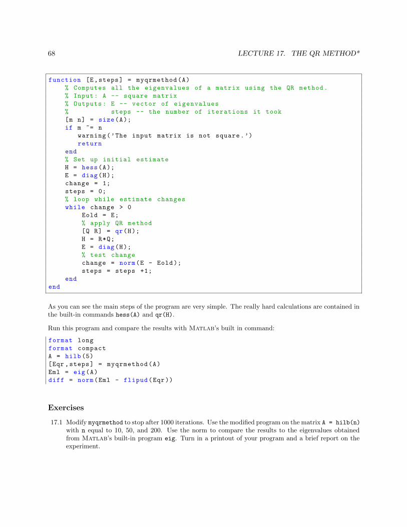
68 LECTURE 17. THE QR METHOD*
function [E,steps] = myqrmethod(A)
% Computes all the eigenvalues of a matrix using the QR method.
% Input: A -- square matrix
% Outputs: E -- vector of eigenvalues
% steps -- the number of iterations it took
[m n] = size(A);
if m ~= n
warning(’The input matrix is not square.’)
return
end
% Set up initial estimate
H = hess(A);
E = diag(H);
change = 1;
steps = 0;
% loop while estimate changes
while change > 0
Eold = E;
% apply QR method
[Q R] = qr(H);
H = R*Q;
E = diag(H);
% test change
change = norm(E - Eold);
steps = steps +1;
end
end
As you can see the main steps of the program are very simple. The really hard calculations are contained inthe built-in commands hess(A) and qr(H).
Run this program and compare the results with Matlab’s built in command:
format long
format compact
A = hilb (5)
[Eqr ,steps] = myqrmethod(A)
Eml = eig(A)
diff = norm(Eml - flipud(Eqr))
Exercises
17.1 Modify myqrmethod to stop after 1000 iterations. Use the modified program on the matrix A = hilb(n)
with n equal to 10, 50, and 200. Use the norm to compare the results to the eigenvalues obtainedfrom Matlab’s built-in program eig. Turn in a printout of your program and a brief report on theexperiment.
Lecture 18
Iterative solution of linear systems*
Newton refinement
Conjugate gradient method
69

Review of Part II
Methods and Formulas
Basic Matrix Theory:
Identity matrix: AI = A, IA = A, and Iv = vInverse matrix: AA−1 = I and A−1A = INorm of a matrix: ‖A‖ ≡ max‖v‖=1 ‖Av‖A matrix may be singular or nonsingular. See Lecture 10.
Solving Process:
Gaussian Elimination produces LU decompositionRow PivotingBack Substitution
Condition number:
cond(A) ≡ max
‖δx‖/‖x‖‖δA‖‖A‖ + ‖δb‖
‖b‖
= max
(Relative error of output
Relative error of inputs
).
A big condition number is bad; in engineering it usually results from poor design.
LU factorization:
PA = LU.
Solving steps:Multiply by P: d = PbForwardsolve: Ly = dBacksolve: Ux = y
Eigenvalues and eigenvectors:
A nonzero vector v is an eigenvector and a number λ is its eigenvalue if
Av = λv.
70
71
Characteristic equation: det(A− λI) = 0Equation of the eigenvector: (A− λI)v = 0Residual for an approximate eigenvector-eigenvalue pair: r = ‖Av − λv‖
Complex eigenvalues:
Occur in conjugate pairs: λ1,2 = α± iβand eigenvectors must also come in conjugate pairs: w = u± iv.
Vibrational modes:
Eigenvalues are frequencies squared. Eigenvectors represent modes.
Power Method:
- Repeatedly multiply x by A and divide by the element with the largest absolute value.- The element of largest absolute value converges to largest absolute eigenvalue.- The vector converges to the corresponding eigenvector.- Convergence assured for a real symmetric matrix, but not for an arbitrary matrix, which may not havereal eigenvalues at all.
Inverse Power Method:
- Apply power method to A−1.- Use solving rather than the inverse.- If λ is an eigenvalue of A then 1/λ is an eigenvalue for A−1.- The eigenvectors for A and A−1 are the same.
Symmetric and Positive definite:
- Symmetric: A = A′.- If A is symmetric its eigenvalues are real.- Positive definite: Ax · x > 0.- If A is positive definite, then its eigenvalues are positive.
QR method:
- Transform A into H the Hessian form of A.- Decompose H in QR.- Multiply Q and R together in reverse order to form a new H.- Repeat- The diagonal of H will converge to the eigenvalues of A.
72 REVIEW OF PART II
Matlab
Matrix arithmetic:
A = [ 1 3 -2 5 ; -1 -1 5 4 ; 0 1 -9 0] . . . . . . . . . . . . . . . . . . . . . . . . . . . . . . Manually enter a matrix.u = [ 1 2 3 4]’
A*u
B = [3 2 1; 7 6 5; 4 3 2]
B*A . . . . . . . . . . . . . . . . . . . . . . . . . . . . . . . . . . . . . . . . . . . . . . . . . . . . . . . . . . . . . . . . . . . . . . . . . . . . . . . . . . multiply B times A.2*A . . . . . . . . . . . . . . . . . . . . . . . . . . . . . . . . . . . . . . . . . . . . . . . . . . . . . . . . . . . . . . . . . . . . . . . . multiply a matrix by a scalar.A + A . . . . . . . . . . . . . . . . . . . . . . . . . . . . . . . . . . . . . . . . . . . . . . . . . . . . . . . . . . . . . . . . . . . . . . . . . . . . . . . . . . . . . . add matrices.A + 3 . . . . . . . . . . . . . . . . . . . . . . . . . . . . . . . . . . . . . . . . . . . . . . . . . . . . . . . . . . . . . . . . . . . add 3 to every entry of a matrix.B.*B . . . . . . . . . . . . . . . . . . . . . . . . . . . . . . . . . . . . . . . . . . . . . . . . . . . . . . . . . . . . . . . . . . . . . . component-wise multiplication.B.^3 . . . . . . . . . . . . . . . . . . . . . . . . . . . . . . . . . . . . . . . . . . . . . . . . . . . . . . . . . . . . . . . . . . . . . component-wise exponentiation.
Special matrices:
I = eye(3) . . . . . . . . . . . . . . . . . . . . . . . . . . . . . . . . . . . . . . . . . . . . . . . . . . . . . . . . . . . . . . . . . . . . . . . . . . . . . . . identity matrixD = ones(5,5)
O = zeros(10,10)
C = rand(5,5) . . . . . . . . . . . . . . . . . . . . . . . . . . . . . . . . . . . . . . . . random matrix with uniform distribution in [0, 1].C = randn(5,5) . . . . . . . . . . . . . . . . . . . . . . . . . . . . . . . . . . . . . . . . . . . . . . . . random matrix with normal distribution.hilb(6)
pascal(5)
General matrix commands:
size(C) . . . . . . . . . . . . . . . . . . . . . . . . . . . . . . . . . . . . . . . . . . . . . . . . . . . . . . . . . . . . . . gives the dimensions (m× n) of A.norm(C) . . . . . . . . . . . . . . . . . . . . . . . . . . . . . . . . . . . . . . . . . . . . . . . . . . . . . . . . . . . . . . . . . . . . gives the norm of the matrix.det(C) . . . . . . . . . . . . . . . . . . . . . . . . . . . . . . . . . . . . . . . . . . . . . . . . . . . . . . . . . . . . . . . . . . . . the determinant of the matrix.max(C) . . . . . . . . . . . . . . . . . . . . . . . . . . . . . . . . . . . . . . . . . . . . . . . . . . . . . . . . . . . . . . . . . . . . . . . . the maximum of each row.min(C) . . . . . . . . . . . . . . . . . . . . . . . . . . . . . . . . . . . . . . . . . . . . . . . . . . . . . . . . . . . . . . . . . . . . . . . . the minimum in each row.sum(C) . . . . . . . . . . . . . . . . . . . . . . . . . . . . . . . . . . . . . . . . . . . . . . . . . . . . . . . . . . . . . . . . . . . . . . . . . . . . . . . . . . . sums each row.mean(C) . . . . . . . . . . . . . . . . . . . . . . . . . . . . . . . . . . . . . . . . . . . . . . . . . . . . . . . . . . . . . . . . . . . . . . . . . the average of each row.diag(C) . . . . . . . . . . . . . . . . . . . . . . . . . . . . . . . . . . . . . . . . . . . . . . . . . . . . . . . . . . . . . . . . . . . . . . just the diagonal elements.inv(C) . . . . . . . . . . . . . . . . . . . . . . . . . . . . . . . . . . . . . . . . . . . . . . . . . . . . . . . . . . . . . . . . . . . . . . . . . . . . . inverse of the matrix.C’ . . . . . . . . . . . . . . . . . . . . . . . . . . . . . . . . . . . . . . . . . . . . . . . . . . . . . . . . . . . . . . . . . . . . . . . . . . . . . . . transpose of the matrix.
Matrix decompositions:
[L U P] = lu(C)
[Q R] = qr(C)
H = hess(C) . . . . . . . . . . transform into a Hessian tri-diagonal matrix, which has the same eigenvalues as A.

Part III
Functions and Data
c©Copyright, Todd Young and Martin Mohlenkamp, Department of Mathematics, Ohio University, 2017
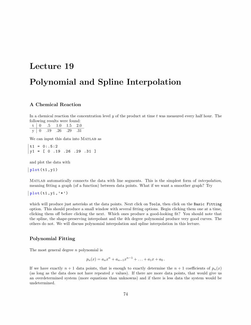
Lecture 19
Polynomial and Spline Interpolation
A Chemical Reaction
In a chemical reaction the concentration level y of the product at time t was measured every half hour. Thefollowing results were found:
t 0 .5 1.0 1.5 2.0y 0 .19 .26 .29 .31
We can input this data into Matlab as
t1 = 0:.5:2
y1 = [ 0 .19 .26 .29 .31 ]
and plot the data with
plot(t1 ,y1)
Matlab automatically connects the data with line segments. This is the simplest form of interpolation,meaning fitting a graph (of a function) between data points. What if we want a smoother graph? Try
plot(t1 ,y1 ,’*’)
which will produce just asterisks at the data points. Next click on Tools, then click on the Basic Fitting
option. This should produce a small window with several fitting options. Begin clicking them one at a time,clicking them off before clicking the next. Which ones produce a good-looking fit? You should note thatthe spline, the shape-preserving interpolant and the 4th degree polynomial produce very good curves. Theothers do not. We will discuss polynomial interpolation and spline interpolation in this lecture.
Polynomial Fitting
The most general degree n polynomial is
pn(x) = anxn + an−1x
n−1 + . . .+ a1x+ a0 .
If we have exactly n + 1 data points, that is enough to exactly determine the n + 1 coefficients of pn(x)(as long as the data does not have repeated x values). If there are more data points, that would give usan overdetermined system (more equations than unknowns) and if there is less data the system would beundetermined.
74
75
Conversely, if we have n data points, then an n− 1 degree polynomial has exactly enough coefficients to fitthe data. This is the case in the example above; there are 5 data points so there is exactly one 4th degreepolynomial that fits the data.
When we tried to use a 5th or higher degree polynomial Matlab returned a warning that the polynomialis not unique since “degree >= number of data points”.
When we tried a lower degree polynomial, we did not get a warning, but we did notice that the resultingcurve does not hit all the data points. If there was an overdetermined system how did Matlab come upwith a pretty good approximation (for cubic)? The answer is the Least Squares Method, which we will studylater.
Predicting the future?
Suppose we want to use the data to extrapolate into the future. Set the plot to the 4th degree polynomial.Then click the Edit button and select the Axes Properties option. A box should appear that allows youto adjust the domain of the x axes. Change the upper limit of the x-axis from 2 to 4. Based on the 4thdegree polynomial, what will the chemical reaction do in the future? Is this reasonable?
Next change from 4th degree polynomial to spline interpolant. According to the spline, what will the chemicalreaction do in the future? Try the shape-preserving interpolant also.
From our (limited) knowledge of chemical reactions, what should be the behavior as time goes on? It shouldreach a limiting value (chemical equilibrium). Could we use the data to predict this equilibrium value? Yes,we could and it is done all the time in many different contexts, but to do so we need to know that there isan equilibrium to predict. This requires that we understand the chemistry of the problem. Thus we havethe following principle: To extrapolate beyond the data, one must have some knowledge of the process.
More data
Generally one would think that more data is better. Input the following data vectors:
t2 = [ 0 .1 .4 .5 .6 1.0 1.4 1.5 1.6 1.9 2.0]
y2 = [ 0 .06 .17 .19 .21 .26 .29 .29 .30 .31 .31]
There are 11 data points, so a 10-th degree polynomial will fit the data. However, this does not give a goodgraph. Thus: A polynomial fit is better for small data sets.
Finally, we note that each data point (xi, yi) gives an equation
pn(xi) = a0 + a1xi + a2x2i + · · ·+ anx
ni = yi.
The unknowns are the coefficients a0, . . . , an. This equation is linear in these unknowns, so determining apolynomial fit requires solving a linear system of equations. This makes polynomial fits quick to calculatesince solving linear systems is what computers do best.

76 LECTURE 19. POLYNOMIAL AND SPLINE INTERPOLATION
A challenging data set
Input the following data set:
x = -4:1:5
y = [ 0 0 0 1 1 1 0 0 0 0]
and plot it:
plot(x,y,’*’)
There are 10 data points, so there is a unique 9 degree polynomial that fits the data. Under Tools andBasic Fitting select the 9th degree polynomial fit. How does it look? De-select the 9th degree polynomialand select the spline interpolant. This should produce a much more satisfactory graph and the shape-preserving spline should be even better. In this section we learn what a spline is.
The idea of a spline
The general idea of a spline is this: on each interval between data points, represent the graph with a simplefunction. The simplest spline is something very familiar to you; it is obtained by connecting the data withlines. Since linear is the most simple function of all, linear interpolation is the simplest form of spline. Thenext simplest function is quadratic. If we put a quadratic function on each interval then we should be ableto make the graph a lot smoother. If we were really careful then we should be able to make the curve smoothat the data points themselves by matching up the derivatives. This can be done and the result is called aquadratic spline. Using cubic functions or 4th degree functions should be smoother still. So, where shouldwe stop? There is an almost universal consensus that cubic is the optimal degree for splines and so we focusthe rest of the lecture on cubic splines.
Cubic spline
Again, the basic idea of the cubic spline is that we represent the function by a different cubic function oneach interval between data points. That is, if there are n data points, then the spline S(x) is the function
S(x) =
C1(x), x0 ≤ x ≤ x1Ci(x), xi−1 ≤ x ≤ xiCn(x), xn−1 ≤ x ≤ xn
(19.1)
where each Ci is a cubic function. The most general cubic function has the form
Ci(x) = ai + bix+ cix2 + dix
3.
To determine the spline we must determine the coefficients, ai, bi, ci, and di for each i. Since there are nintervals, there are 4n coefficients to determine. First we require that the spline be exact at the data:
Ci(xi−1) = yi−1 and Ci(xi) = yi, (19.2)
at every data point. In other words,
ai + bixi−1 + cix2i−1 + dix
3i−1 = yi−1 and ai + bixi + cix
2i + dix
3i = yi.

77
Notice that there are 2n of these conditions. Then to make S(x) as smooth as possible we require
C ′i(xi) = C ′i+1(xi) and
C ′′i (xi) = C ′′i+1(xi)(19.3)
at all the internal points, i.e. x1, x2, x3, . . . , xn−1. In terms of the points these conditions can be written as
bi + 2cixi + 3dix2i = bi+1 + 2ci+1xi + 3di+1x
2i and
2ci + 6dixi = 2ci+1 + 6di+1xi.(19.4)
There are 2(n − 1) of these conditions. Since each Ci is cubic, there are a total of 4n coefficients in theformula for S(x). So far we have 4n − 2 equations, so we are 2 equations short of being able to determineall the coefficients. At this point we have to make a choice. The usual choice is to require
C ′′1 (x0) = C ′′n(xn) = 0. (19.5)
These are called natural or simple boundary conditions. The other common option is called clamped boundaryconditions:
C ′1(x0) = C ′n(xn) = 0. (19.6)
The terminology used here is obviously parallel to that used for beams. That is not the only parallel betweenbeams and cubic splines. It is an interesting fact that a cubic spline is exactly the shape of a (linear) beamrestrained to match the data by simple supports.
Note that the equations above are all linear equations with respect to the unknowns (coefficients). Thisfeature makes splines easy to calculate since solving linear systems is what computers do best.
Exercises
19.1 You are given the following data:
t = [ 0 .1 .499 .5 .6 1.0 1.4 1.5 1.899 1.9 2.0 ]
y = [ 0 .06 .17 .19 .21 .26 .29 .29 .30 .31 .31 ]
(a) Plot the data, using ”*” at the data points, then try a polynomial fit of the correct degree tointerpolate this number of data points: What do you observe. Give an explanation of this error,in particular why is the term badly conditioned used?
(b) Plot the data along with a spline interpolant. How does this compare with the plot above? Whatis a way to make the plot better?
Lecture 20
Least Squares Fitting: Noisy Data
Very often data has a significant amount of noise. The least squares approximation is intentionally well-suited to represent noisy data. The next illustration shows the effects noise can have and how least squaresis used.
Traffic flow model
Suppose you are interested in the time it takes to travel on a certain section of highway for the sake of plan-ning. According to theory, assuming up to a moderate amount of traffic, the time should be approximately
T (x) = ax+ b
where b is the travel time when there is no other traffic, and x is the current number of cars on the road (inhundreds). To determine the coefficients a and b you could run several experiments which consist of drivingthe highway at different times of day and also estimating the number of cars on the road using a counter.Of course both of these measurements will contain noise, i.e. random fluctuations.
We could simulate such data in Matlab as follows:
x = 1:.1:6;
T = .1*x + 1;
Tn = T + .1* randn(size(x));
plot(x,Tn ,’.’)
The data should look like it lies on a line, but with noise. Click on the Tools button and choose Basic fitting.Then choose a linear fit. The resulting line should go through the data in what looks like a very reasonableway. Click on show equations. Compare the equation with T (x) = .1x + 1. The coefficients should bepretty close considering the amount of noise in the plot. Next, try to fit the data with a spline. The resultshould be ugly. We can see from this example that splines are not suited to noisy data.
How does Matlab obtain a very nice line to approximate noisy data? The answer is a very standardnumerical/statistical method known as least squares.
Linear least squares
Consider in the previous example that we wish to fit a line to a lot of data that does not exactly lie on aline. For the equation of the line we have only two free coefficients, but we have many data points. We can
78
79
not possibly make the line go through every data point, we can only wish for it to come reasonably close toas many data points as possible. Thus, our line must have an error with respect to each data point. If `(x)is our line and (xi, yi) are the data, then
ei = yi − `(xi)
is the error of ` with respect to each (xi, yi). To make `(x) reasonable, we wish to simultaneously minimizeall the errors: e1, e2, . . . , en. There are many possible ways one could go about this, but the standard oneis to try to minimize the sum of the squares of the errors. That is, we denote by E the sum of the squares:
E =
n∑i=1
(yi − `(xi))2 =
n∑i=1
(yi − axi − b)2 . (20.1)
In the above expression xi and yi are given, but we are free to choose a and b, so we can think of E as afunction of a and b, i.e. E(a, b). In calculus, when one wishes to find a minimum value of a function of twovariables, we set the partial derivatives equal to zero:
∂E∂a
= −2
n∑i=1
(yi − axi − b)xi = 0
∂E∂b
= −2
n∑i=1
(yi − axi − b) = 0.
(20.2)
We can simplify these equations to obtain(n∑i=1
x2i
)a+
(n∑i=1
xi
)b =
n∑i=1
xiyi and(n∑i=1
xi
)a+ nb =
n∑i=1
yi.
(20.3)
Thus, the whole problem reduces to a 2 by 2 linear system to find the coefficients a and b. The entries inthe matrix are determined from simple formulas using the data. The process is quick and easily automated,which is one reason it is very standard.
We could use the same process to obtain a quadratic or higher polynomial fit to data. If we try to fit ann degree polynomial, the software has to solve an n × n linear system, which is easily done. This is whatMatlab’s basic fitting tool uses to obtain an n degree polynomial fit whenever the number of data pointsis more than n+ 1.
Drag coefficients
Drag due to air resistance is proportional to the square of the velocity, i.e. d = kv2. In a wind tunnelexperiment the velocity v can be varied by setting the speed of the fan and the drag can be measureddirectly (it is the force on the object). In this and every experiment some random noise will occur. Thefollowing sequence of commands replicates the data one might receive from a wind tunnel:
v = 0:1:60;
d = .1234*v.^2;
dn = d + .4*v.* randn(size(v));
plot(v,dn ,’*’)
80 LECTURE 20. LEAST SQUARES FITTING: NOISY DATA
The plot should look like a quadratic, but with some noise. Using the tools menu, add a quadratic fit andenable the “show equations” option. What is the coefficient of x2? How close is it to 0.1234?
Note that whenever you select a polynomial in Matlab with a degree less than n− 1 Matlab will producea least squares fit.
You will notice that the quadratic fit includes both a constant and linear term. We know from the physicalsituation that these should not be there; they are remnants of noise and the fitting process. Since we knowthe curve should be kv2, we can do better by employing that knowledge. For instance, we know that thegraph of d versus v2 should be a straight line. We can produce this easily:
z = v.^2;
plot(z,dn ,’*’)
By changing the independent variable from v to z = v2 we produced a plot that looks like a line with noise.Add a linear fit. What is the linear coefficient? This should be closer to 0.1234 than using a quadratic fit.
The second fit still has a constant term, which we know should not be there. If there was no noise, thenat every data point we would have k = d/v2. We can express this as a linear system z’*k = dn’, which isbadly overdetermined since there are more equations than unknowns. Since there is noise, each point willgive a different estimate for k. In other words, the overdetermined linear system is also inconsistent. WhenMatlab encounters such systems, it automatically gives a least squares solution of the matrix problem,i.e. one that minimizes the sum of the squared errors, which is exactly what we want. To get the leastsquares estimate for k, do
k = z’\dn’
This will produce a number close to .1234.
Note that this is an application where we have physical knowledge. In this situation extrapolation would bemeaningful. For instance we could use the plot to find the predicted drag at 80 mph.
Exercises
20.1 Find two tables of data in an engineering textbook or engineering website. Plot each (with ”*” at datapoints) and decide if the data is best represented by a polynomial interpolant, spline interpolant, orleast squares fit polynomial. Label the axes and include a title. Turn in the best plot of each. Indicatethe source and meaning of the data.
20.2 The following table contains information from a chemistry experiment in which the concentration ofa product was measured at one minute intervals.
T 0 1 2 3 4 5 6 7C 3.033 3.306 3.672 3.929 4.123 4.282 4.399 4.527
Plot this data. Suppose it is known that this chemical reaction should follow the law: c = a −b exp(−0.2t). Following the example in the notes about the drag coefficients, change one of thevariables so that the law is a linear function. Then plot the new variables and use the linear fitoption to estimate a and b. What will be the eventual concentration? Finally, plot the graph ofa− b exp(−0.2t) on the interval [0,10] (as a solid curve), along with the data (using ’*’).
Lecture 21
Integration: Left, Right and Trapezoid Rules
The Left and Right endpoint rules
In this section, we wish to approximate a definite integral∫ b
a
f(x) dx ,
where f(x) is a continuous function. In calculus we learned that integrals are (signed) areas and can beapproximated by sums of smaller areas, such as the areas of rectangles. We begin by choosing points xithat subdivide [a, b]:
a = x0 < x1 < . . . < xn−1 < xn = b.
The subintervals [xi−1, xi] determine the width ∆xi of each of the approximating rectangles. For the height,we learned that we can choose any height of the function f(x∗i ) where x∗i ∈ [xi−1, xi]. The resultingapproximation is ∫ b
a
f(x) dx ≈n∑i=1
f(x∗i )∆xi.
To use this to approximate integrals with actual numbers, we need to have a specific x∗i in each interval.The two simplest (and worst) ways to choose x∗i are as the left-hand point or the right-hand point of eachinterval. This gives concrete approximations which we denote by Ln and Rn given by
Ln =n∑i=1
f(xi−1)∆xi and Rn =n∑i=1
f(xi)∆xi .
function L = myleftsum(x,y)
% produces the left sum from data input.
% Inputs: x -- vector of the x coordinates of the partition
% y -- vector of the corresponding y coordinates
% Output: returns the approximate integral
n = length(x);
L = 0;
for i = 1:n-1
% accumulate height times width
L = L + y(i)*(x(i+1) - x(i));
end
end
81

82 LECTURE 21. INTEGRATION: LEFT, RIGHT AND TRAPEZOID RULES
-
6
-
6
Figure 21.1: The left and right sums, Ln and Rn.
Often we can take xi to be evenly spaced, with each interval having the same width:
h =b− an
,
where n is the number of subintervals. If this is the case, then Ln and Rn simplify to
Ln =b− an
n−1∑i=0
f(xi) and (21.1)
Rn =b− an
n∑i=1
f(xi). (21.2)
The foolishness of choosing left or right endpoints is illustrated in Figure 21.1. As you can see, for a verysimple function like f(x) = 1 + .5x, each rectangle of Ln is too short, while each rectangle of Rn is too tall.This will hold for any increasing function. For decreasing functions Ln will always be too large while Rnwill always be too small.
The Trapezoid rule
Knowing that the errors of Ln and Rn are of opposite sign, a very reasonable way to get a better approxi-mation is to take an average of the two. We will call the new approximation Tn:
Tn =Ln +Rn
2.
This method also has a straight-forward geometric interpretation. On each subrectangle we are using
Ai =f(xi−1) + f(xi)
2∆xi ,
which is exactly the area of the trapezoid with sides f(xi−1) and f(xi). We thus call the method the trapezoidmethod. See Figure 21.2. We can rewrite Tn as

83
-
6
HHHHH
HHH
HH
Figure 21.2: The trapezoid rule, Tn.
Tn =
n∑i=1
f(xi−1) + f(xi)
2∆xi.
In the evenly spaced case, we can write this as
Tn =b− a2n
(f(x0) + 2f(x1) + . . .+ 2f(xn−1) + f(xn)
). (21.3)
Caution: The convention used here is to begin numbering the points at 0, i.e. x0 = a; this allows n to be thenumber of subintervals and the index of the last point xn. However, Matlab’s indexing convention beginsat 1. Thus, when programming in Matlab, the first entry in x will be x0, i.e. x(1)= x0 and x(n+1)= xn.
If we are given data about the function, rather than a formula for the function, often the data are not evenlyspaced. The following function program could then be used.
function T = mytrap(x,y)
% Calculates the Trapezoid rule approximation of the integral from data
% Inputs: x -- vector of the x coordinates of the partitian
% y -- vector of the corresponding y coordinates
% Output: returns the approximate integral
n = length(x);
T = 0;
for i = 1:n-1
% accumulate the signed area of the trapezoids
T = T + .5*(y(i)+y(i+1))*(x(i+1) - x(i));
end
end

84 LECTURE 21. INTEGRATION: LEFT, RIGHT AND TRAPEZOID RULES
Using the Trapezoid rule for areas in the plane
In multi-variable calculus you were supposed to learn that you can calculate the area of a region R in theplane by calculating the line integral
A = −∮C
y dx , (21.4)
where C is the counter-clockwise curve around the boundary of the region. We can represent such a curveby consecutive points on it, i.e. x = (x0, x1, x2, . . . , xn−1, xn), and y = (y0, y1, y2, . . . , yn−1, yn). Since weare assuming the curve ends where it begins, we require (xn, yn) = (x0, y0). Applying the trapezoid methodto the integral (21.4) gives
A = −n∑i=1
yi−1 + yi2
(xi − xi−1) .
This formula then is the basis for calculating areas when coordinates of boundary points are known, but notnecessarily formulas for the boundaries such as in a land survey.
In the following script, we can use this method to approximate the area of a unit circle using n points onthe circle:
% Calculates pi using a trapezoid approximation of the unit circle.
format long
n = 10;
t = linspace (0,2*pi,n+1);
x = cos(t);
y = sin(t);
plot(x,y)
A = 0
for i = 1:n
A = A - (y(i)+y(i+1))*(x(i+1)-x(i))/2;
end
A
Vector Operations using Slicing and Summing
In the programs above we used loops to explicitly accumulate sums. For example, in mytrap we had
T = 0;
for i = 1:n-1
T = T + .5*(y(i)+y(i+1))*(x(i+1) - x(i));
end
The alternative is to use vector operations by taking slices out of the vectors and using the sum function.We can replace the above code by
T = .5*sum( (y(1:n-1)+y(2:n)) .* (x(2:n)-x(1:n-1)) );
Generally, explicit loops are easier to understand but vector operations are more efficient and compact.

85
Exercises
21.1 For the integral∫ 2
1
√x dx calculate L4, R4, and T4 with even spacing (by hand, but use a calculator)
using formulas (21.1), (21.2) and (21.3). Find the percentage error of these approximations, using theexact value.
21.2 Write a well-commented Matlab function program myints whose inputs are f , a, b and n and whoseoutputs are L, R and T , the left, right and trapezoid integral approximations for f on [a, b] with nsubintervals. To make it efficient, use x = linspace(a,b,n+1) to make the x values, y = f(x) tomake the y values, slice and sum to add the 2nd to nth y entries once, and then add on the missingterms to obtain the left, right and trapezoid approximations. Also take advantage of the fact that ∆xiis constant.
Change to format long and apply your program to the integral∫ 2
1
√x dx. Compare with the results of
the previous exercise. Also find L100, R100 and T100 and the percentage errors of these approximations.
Turn in the program and a brief summary of the results.

Lecture 22
Integration: Midpoint and Simpson’s Rules
Midpoint rule
If we use the endpoints of the subintervals to approximate the integral, we run the risk that the values at theendpoints do not accurately represent the average value of the function on the subinterval. A point which ismuch more likely to be close to the average would be the midpoint of each subinterval. Using the midpointin the sum is called the midpoint rule. On the i-th interval [xi−1, xi] we will call the midpoint xi, i.e.
xi =xi−1 + xi
2.
If ∆xi = xi − xi−1 is the length of each interval, then using midpoints to approximate the integral wouldgive the formula
Mn =
n∑i=1
f(xi)∆xi .
For even spacing, ∆x = (b− a)/n, and the formula is
Mn =b− an
n∑i=1
f(xi) =b− an
(y1 + y2 + . . .+ yn), (22.1)
where we define yi = f(xi).
While the midpoint method is obviously better than Ln or Rn, it is not obvious that it is actually betterthan the trapezoid method Tn, but it is.
Simpson’s rule
Consider Figure 22.1. If f is not linear on a subinterval, then it can be seen that the errors for the midpointand trapezoid rules behave in a very predictable way, they have opposite sign. For example, if the functionis concave up then Tn will be too high, while Mn will be too low. Thus it makes sense that a better estimatewould be to average Tn and Mn. However, in this case we can do better than a simple average. The errorwill be minimized if we use a weighted average. To find the proper weight we take advantage of the fact thatfor a quadratic function the errors EMn and ETn are exactly related by
|EMn| =1
2|ETn| .
86

87
-
6
u
Figure 22.1: Comparing the trapezoid and midpoint method on a single subinterval. The functionis concave up, in which case Tn is too high, while Mn is too low.
Thus we take the following weighted average of the two, which is called Simpson’s rule:
S2n =2
3Mn +
1
3Tn .
If we use this weighting on a quadratic function the two errors will exactly cancel.
Notice that we write the subscript as 2n. That is because we usually think of 2n subintervals in theapproximation; the n subintervals of the trapezoid are further subdivided by the midpoints. We can thennumber all the points using integers. If we number them this way we notice that the number of subintervalsmust be an even number.
The formula for Simpson’s rule if the subintervals are evenly spaced is the following (with n intervals, wheren is even):
Sn =b− a3n
(f(x0) + 4f(x1) + 2f(x2) + 4f(x3) + . . .+ 2f(xn−2) + 4f(xn−1) + f(xn)) .
Note that if we are presented with data xi, yi where the xi points are evenly spaced with xi+1 − xi = ∆x,it is easy to apply Simpson’s method:
Sn =∆x
3(y0 + 4y1 + 2y2 + 4y3 + . . .+ 2yn−2 + 4yn−1 + yn) . (22.2)
Notice the pattern of the coefficients. The following program will produce these coefficients for n intervals,if n is an even number. Try it for n = 6, 7, 100.

88 LECTURE 22. INTEGRATION: MIDPOINT AND SIMPSON’S RULES
function w = mysimpweights(n)
% Computes the weights for Simpson ’s rule
% Input: n -- the number of intervals , must be even
% Output: w -- a (column) vector with the weights , length n+1
if rem(n,2) ~= 0
error(’n must be even for Simpsons rule’)
end
w = ones(n+1 ,1); % column vector , starts all 1
for i = 2:n
% loop except for first and last , which stay 1
if rem(i ,2)==0
w(i)=4; % even index values set to 4
else
w(i)=2; % odd index values set to 4
end
end
end
Simpson’s rule is incredibly accurate. We will consider just how accurate in the next section. The onedrawback is that the points used must either be evenly spaced, or at least the odd number points mustlie exactly at the midpoint between the even numbered points. In applications where you can choose thespacing, this is not a problem. In applications such as experimental or simulated data, you might not havecontrol over the spacing and then you cannot use Simpson’s rule.
Error bounds
The trapezoid, midpoint, and Simpson’s rules are all approximations. As with any approximation, before youcan safely use it, you must know how good (or bad) the approximation might be. For these methods thereare formulas that give upper bounds on the error. In other words, the worst case errors for the methods.These bounds are given by the following statements:
• Suppose f ′′ is continuous on [a,b]. Let K2 = maxx∈[a,b] |f ′′(x)|. Then the errors ETn and EMn of the
Trapezoid and Midpoint rules, respectively, applied to∫ baf dx satisfy
|ETn| ≤K2(b− a)3
12n2=K2(b− a)
12∆x2 and
|EMn| ≤K2(b− a)3
24n2=K2(b− a)
24∆x2 .
• Suppose f (4) is continuous on [a,b]. Let K4 = maxx∈[a,b] |f (4)(x)|. Then the error ESn of Simpson’s
rule applied to∫ baf dx satisfies
|ESn| ≤K4(b− a)5
180n4=K4(b− a)
180∆x4.
In practice K2 and K4 are themselves approximated from the values of f at the evaluation points.
89
The most important thing in these error bounds is the last term. For the trapezoid and midpoint method,the error depends on ∆x2 whereas the error for Simpson’s rule depends on ∆x4. If ∆x is just moderatelysmall, then there is a huge advantage with Simpson’s method.
When an error depends on a power of a parameter, such as above, we sometimes use the order notation. Inthe above error bounds we say that the trapezoid and midpoint rules have errors of order O(∆x2), whereasSimpson’s rule has error of order O(∆x4).
In Matlab there is a built-in command for definite integrals: integral(f,a,b) where the f is a functionand a and b are the endpoints. The command uses “adaptive Simpson quadrature”, a form of Simpson’srule that checks its own accuracy and adjusts the grid size where needed. Here is an example of its usage:
f = @(x) x.^(1/3).* sin(x.^3)
I = integral(f,0,1)
Exercises
22.1 Using formulas (22.1) and (22.2), for the integral∫ 2
1
√x dx calculate M4 and S4 (by hand, but use
a calculator and a lot of digits). Find the percentage error of these approximations, using the exactvalue. Compare with exercise 21.1.
22.2 Write a well-commented Matlab function program mymidpoint that calculates the midpoint ruleapproximation for
∫f on the interval [a, b] with n subintervals. The inputs should be f , a, b and n.
Use your program on the integral∫ 2
1
√x dx to obtain M4 and M100. Compare these with exercise 22.1
and the true value of the integral.
22.3 Write a well-commented Matlab function program mysimpson that calculates the Simpson’s rule ap-proximation for
∫f on the interval [a, b] with n subintervals. It should call the program mysimpweights
to produce the coefficients. Use your program on the integral∫ 2
1
√x dx to obtain S4 and S100. Compare
these with exercise 22.1, exercise 22.2, and the true value of the integral.
Lecture 23
Plotting Functions of Two Variables
Functions on Rectangular Grids
Suppose you wish to plot a function f(x, y) on the rectangle a ≤ x ≤ b and c ≤ y ≤ d. The graph of afunction of two variables is of course a three dimensional object. Visualizing the graph is often very useful.
For example, suppose you have a formula
f(x, y) = x sin(xy)
and you are interested in the function on the region 0 ≤ x ≤ 5, π ≤ y ≤ 2π. A way to plot this function inMatlab would be the following sequence of commands:
f = @(x,y) x.*sin(x.*y)
[X,Y] = meshgrid (0:.1:5 ,pi:.01* pi:2*pi);
Z = f(X,Y)
mesh(X,Y,Z)
This will produce a 3-D plot that you can rotate by clicking on the rotate icon and then dragging with themouse. Instead of the command mesh, you could use the command
surf(X,Y,Z)
The key command in this sequence is [X Y] = meshgrid(a:h:b,c:k:d), which produces matrices of x andy values in X and Y. Enter:
size(X)
size(Y)
size(Z)
to see that each of these variables is a 101× 51 matrix. To see the first few entries of X enter
X(1:6 ,1:6)
and to see the first few values of Y type
Y(1:6 ,1:6)
You should observe that the x values in X begin at 0 on the left column and increase from left to right. The yvalues on the other have start at π at the top and increase from top to bottom. Note that this arrangementis flipped from the usual arrangment in the x-y plane.
90
91
In the command [X Y] = meshgrid(a:h:b,c:k:d), h is the increment in the x direction and k is theincrement in the y direction. Often we will calculate
h =b− am
and k =d− cn
,
where m is the number of intervals in the x direction and n is the number of intervals in the y direction. Toobtain a good plot it is best if m and n can be set between 10 and 100.
For another example of how meshgrid works, try the following and look at the output in X and Y.
[X,Y] = meshgrid (0:.5:4 ,1:.2:2);
Scattered Data and Triangulation
Often we are interested in objects whose bases are not rectangular. For instance, data does not usually comearranged in a nice rectangular grid; rather, measurements are taken where convenient.
In Matlab we can produce triangles for a region by recording the coordinates of the vertices and recordingwhich vertices belong to each triangle. The following script program produces such a set of triangles:
% mytriangles
% Program to produce a triangulation.
% V contains vertices , which are (x,y) pairs
V = [ 1/2 1/2 ; 1 1 ; 3/2 1/2 ; .5 1.5 ; 0 0
1 0 ; 2 0 ; 2 1 ; 1.5 1.5 ; 1 2
0 2 ; 0 1]
% x, y are row vectors containing coordinates of vertices
x = V(:,1)’;
y = V(:,2)’;
% Assign the triangles
T = delaunay(x,y)
You can plot the triangles using
trimesh(T,x,y)
You can also prescribe values (heights) at each vertex directly (say from a survey):
z1 = [ 2 3 2.5 2 1 1 .5 1.5 1.6 1.7 .9 .5 ];
or using a function:
f = @(x,y) abs(sin(x.*y)).^(3/2);
z2 = f(x,y);
The resulting profiles can be plotted:
trimesh(T,x,y,z1)
trisurf(T,x,y,z2)

92 LECTURE 23. PLOTTING FUNCTIONS OF TWO VARIABLES
Each row of the matrix T corresponds to a triangle, so T(i,:) gives triangle number i. The three cornersof triangle number i are at indices T(i,1), T(i,2), and T(i,3). So for example to get the y-coordinate ofthe second point of triangle number 5, enter
y(T(5 ,2))
To see other examples of regions defined by triangle get mywedge.m and mywasher.m from the web site andrun them. Each of these programs defines vectors x and y of x and y values of vertices and a matrix T. Asbefore T is a list of sets of three integers. Each triple of integers indicates which vertices to connect in atriangle.
To plot a function, say f(x, y) = x2 − y2 on the washer figure try
mywasher
z = x.^2 - y.^2
trisurf(T,x,y,z)
Note again that this plot can be rotated using the icon and mouse.
Exercises
23.1 Plot the function f(x, y) = xe−x2−y2 on the rectangle −3 ≤ x ≤ 3, −2 ≤ y ≤ 2 using meshgrid and
mesh. Make an appropriate choice of m and n and if necessary a rotation to produce a good plot.Calculate the h and k corresponding to your m and n. Turn in your plot and the calculation of h andk.
23.2 Modeling after mywasher.m, produce
@@@
@@@
HHHH
HHUse the axis command to zoom out so the outside edges are clearly visible.
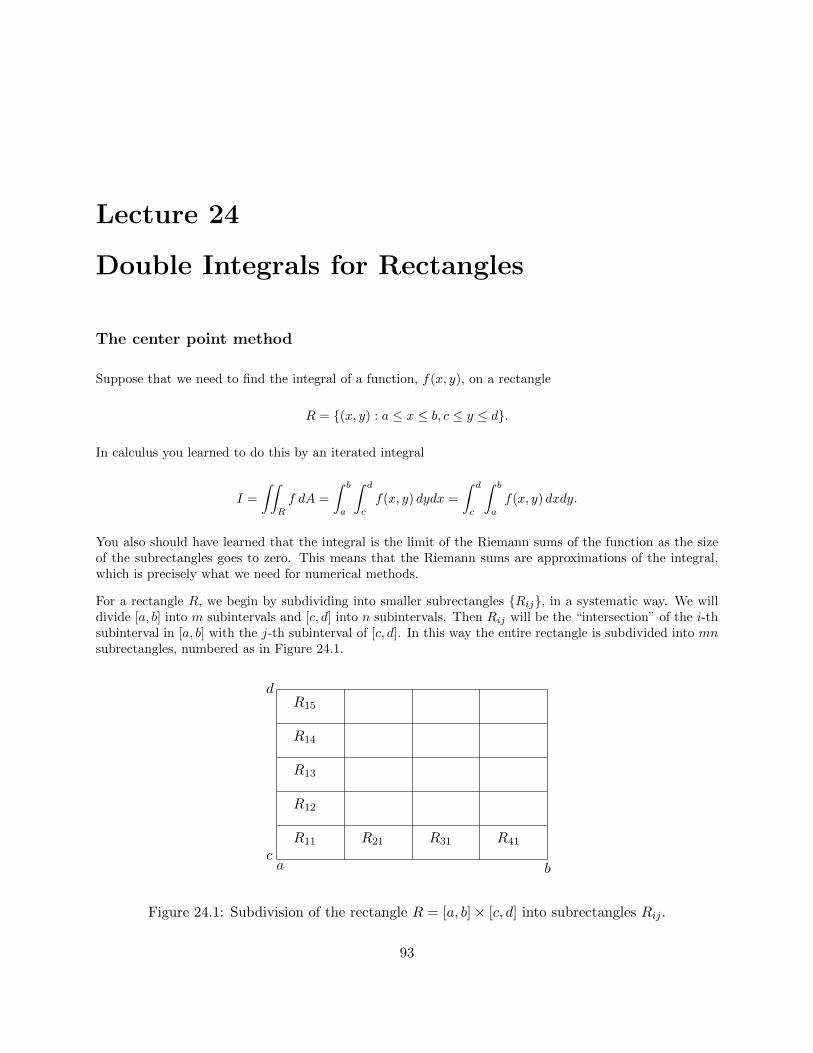
Lecture 24
Double Integrals for Rectangles
The center point method
Suppose that we need to find the integral of a function, f(x, y), on a rectangle
R = (x, y) : a ≤ x ≤ b, c ≤ y ≤ d.
In calculus you learned to do this by an iterated integral
I =
∫∫R
f dA =
∫ b
a
∫ d
c
f(x, y) dydx =
∫ d
c
∫ b
a
f(x, y) dxdy.
You also should have learned that the integral is the limit of the Riemann sums of the function as the sizeof the subrectangles goes to zero. This means that the Riemann sums are approximations of the integral,which is precisely what we need for numerical methods.
For a rectangle R, we begin by subdividing into smaller subrectangles Rij, in a systematic way. We willdivide [a, b] into m subintervals and [c, d] into n subintervals. Then Rij will be the “intersection” of the i-thsubinterval in [a, b] with the j-th subinterval of [c, d]. In this way the entire rectangle is subdivided into mnsubrectangles, numbered as in Figure 24.1.
a bc
d
R11 R21 R31 R41
R12
R13
R14
R15
Figure 24.1: Subdivision of the rectangle R = [a, b]× [c, d] into subrectangles Rij .
93
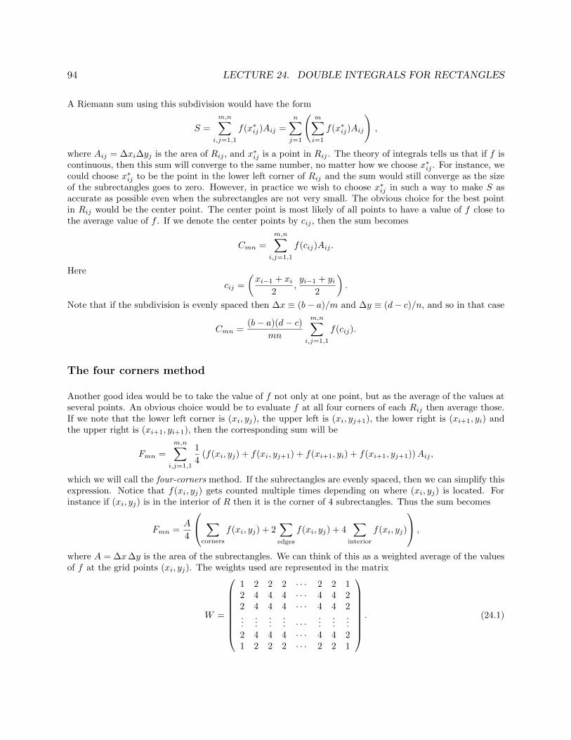
94 LECTURE 24. DOUBLE INTEGRALS FOR RECTANGLES
A Riemann sum using this subdivision would have the form
S =
m,n∑i,j=1,1
f(x∗ij)Aij =
n∑j=1
(m∑i=1
f(x∗ij)Aij
),
where Aij = ∆xi∆yj is the area of Rij , and x∗ij is a point in Rij . The theory of integrals tells us that if f iscontinuous, then this sum will converge to the same number, no matter how we choose x∗ij . For instance, wecould choose x∗ij to be the point in the lower left corner of Rij and the sum would still converge as the sizeof the subrectangles goes to zero. However, in practice we wish to choose x∗ij in such a way to make S asaccurate as possible even when the subrectangles are not very small. The obvious choice for the best pointin Rij would be the center point. The center point is most likely of all points to have a value of f close tothe average value of f . If we denote the center points by cij , then the sum becomes
Cmn =
m,n∑i,j=1,1
f(cij)Aij .
Here
cij =
(xi−1 + xi
2,yi−1 + yi
2
).
Note that if the subdivision is evenly spaced then ∆x ≡ (b− a)/m and ∆y ≡ (d− c)/n, and so in that case
Cmn =(b− a)(d− c)
mn
m,n∑i,j=1,1
f(cij).
The four corners method
Another good idea would be to take the value of f not only at one point, but as the average of the values atseveral points. An obvious choice would be to evaluate f at all four corners of each Rij then average those.If we note that the lower left corner is (xi, yj), the upper left is (xi, yj+1), the lower right is (xi+1, yi) andthe upper right is (xi+1, yi+1), then the corresponding sum will be
Fmn =
m,n∑i,j=1,1
1
4(f(xi, yj) + f(xi, yj+1) + f(xi+1, yi) + f(xi+1, yj+1))Aij ,
which we will call the four-corners method. If the subrectangles are evenly spaced, then we can simplify thisexpression. Notice that f(xi, yj) gets counted multiple times depending on where (xi, yj) is located. Forinstance if (xi, yj) is in the interior of R then it is the corner of 4 subrectangles. Thus the sum becomes
Fmn =A
4
∑corners
f(xi, yj) + 2∑edges
f(xi, yj) + 4∑
interior
f(xi, yj)
,
where A = ∆x∆y is the area of the subrectangles. We can think of this as a weighted average of the valuesof f at the grid points (xi, yj). The weights used are represented in the matrix
W =
1 2 2 2 · · · 2 2 12 4 4 4 · · · 4 4 22 4 4 4 · · · 4 4 2...
......
... · · ·...
......
2 4 4 4 · · · 4 4 21 2 2 2 · · · 2 2 1
. (24.1)

95
We could implement the four-corner method by forming a matrix (fij) of f values at the grid points, thendoing entry-wise multiplication of the matrix with the weight matrix. Then the integral would be obtainedby summing all the entries of the resulting matrix and multiplying that by A/4. The formula would be
Fmn =(b− a)(d− c)
4mn
m+1,n+1∑i,j=1,1
Wijf(xi, yj).
Notice that the four-corners method coincides with applying the trapezoid rule in each direction. Thus it isin fact a double trapezoid rule.
The double Simpson method
The next improvement one might make would be to take an average of the center point sum Cmn and thefour corners sum Fmn. However, a more standard way to obtain a more accurate method is the Simpsondouble integral. It is obtained by applying Simpson’s rule for single integrals to the iterated double integral.The resulting method requires that both m and n be even numbers and the grid be evenly spaced. If this isthe case we sum up the values f(xi, yj) with weights represented in the matrix
W =
1 4 2 4 · · · 2 4 14 16 8 16 · · · 8 16 42 8 4 8 · · · 4 8 24 16 8 16 · · · 8 16 4...
......
... · · ·...
......
2 8 4 8 · · · 4 8 24 16 8 16 · · · 8 16 41 4 2 4 · · · 2 4 1
. (24.2)
The sum of the weighted values is multiplied by A/9 and the formula is
Smn =(b− a)(d− c)
9mn
m+1,n+1∑i,j=1,1
Wijf(xi, yj).
Matlab has a built in command for double integrals on rectangles: integral2(f,a,b,c,d). Here is anexample:
f = @(x,y) sin(x.*y)./ sqrt(x+y)
I = integral2(f,0.5 ,1 ,0.5 ,2)
Below is a Matlab function which will produce the matrix of weights needed for Simpson’s rule for doubleintegrals. It uses the function mysimpweights from Lecture 22.

96 LECTURE 24. DOUBLE INTEGRALS FOR RECTANGLES
function W = mydblsimpweights(m,n)
% Return the matrix of weights for Simpson ’s rule for double integrals.
% Inputs: m -- number of intervals in the row direction.
% must be even.
% n -- number of intervals in the column direction.
% must be even.
% Output: W -- a (m+1)x(n+1) matrix of the weights
if rem(m ,2)~=0 || rem(n ,2)~=0
error(’m and n must be even for Simpsons rule’)
end
% get 1-dimensional weights
u = mysimpweights(m);
v = mysimpweights(n);
W = u*v’;
end
Exercises
24.1 Download the program mylowerleft from the web site. Modify it to make a new program mycenter
that does the center point method. Implement the change by changing the “meshgrid” to put the gridpoints at the centers of the subrectangles. Look at the mesh plot produced to make sure the programis putting the grid where you want it. Use both programs to approximate the integral∫ 2
0
∫ 5
1
√xy dy dx,
using (m,n) = (10, 18). Evaluate this integral exactly (by hand) and compare the accuracy of the twoprograms.
24.2 Write a well-commented Matlab function program mydblsimp that computes the Simpson’s ruleapproximation. Let it call the program mydblsimpweights to make the weight matrix (24.2). Checkthe program on the integral in the previous problem using (m,n) = (10, 18) and (m,n) = (100, 100).
24.3 Using mysimpweights and mydblsimpweights as models make well-commented Matlab functionprograms mytrapweights and mydbltrapweights that will produce the weights for the trapezoid ruleand the weight matrix for the four corners (double trapezoid) method (24.1). Turn in the programsand the resulting weights for a 5× 6 grid.

Lecture 25
Double Integrals for Non-rectangles
In the previous lecture we considered only integrals over rectangular regions. In practice, regions of interestare rarely rectangles and so in this lecture we consider two strategies for evaluating integrals over otherregions.
Redefining the function
One strategy is to redefine the function so that it is zero outside the region of interest, then integrate overa rectangle that includes the region.
For example, suppose we need to approximate the value of
I =
∫∫T
sin3(xy) dx dy
where T is the triangle with corners at (0, 0), (1, 0) and (0, 2). Then we could let R be the rectangle[0, 1] × [0, 2] which contains the triangle T . Notice that the hypotenuse of the triangle has the equation2x+ y = 2. Then make f(x) = sin3(xy) if 2x+ y ≤ 2 and f(x) = 0 if 2x+ y > 2. In Matlab we can makethis function with the command
f = @(x,y) sin(x.*y).^3.*(2*x + y <= 2)
In this command <= is a logical command. The term in parentheses is then a logical statement and is giventhe value 1 if the statement is true and 0 if it is false. We can then integrate the modified f on [0, 1]× [0, 2]using the command
I = integral2(f,0,1,0,2)
As another example, suppose we need to integrate 10000 + x2 exp(xy) inside the circle of radius 2 centeredat (1, 2). The equation for this circle is (x − 1)2 + (y − 2)2 = 4. Note that the inside of the circle is(x− 1)2 + (y − 2)2 ≤ 4 and that the circle is contained in the rectangle [−1, 3]× [0, 4]. Thus we can createthe right function, plot it, and integrate it by
f = @(x,y) (10+(x -1).*(y -2)).*((x -1).^2 + (y -2).^2 <= 4)
[X Y] = meshgrid ( -4:0.01:4 , -3:0.01:5);
Z = f(X,Y);
mesh(X,Y,Z)
I = integral2(f,-1,3,0,4)
97
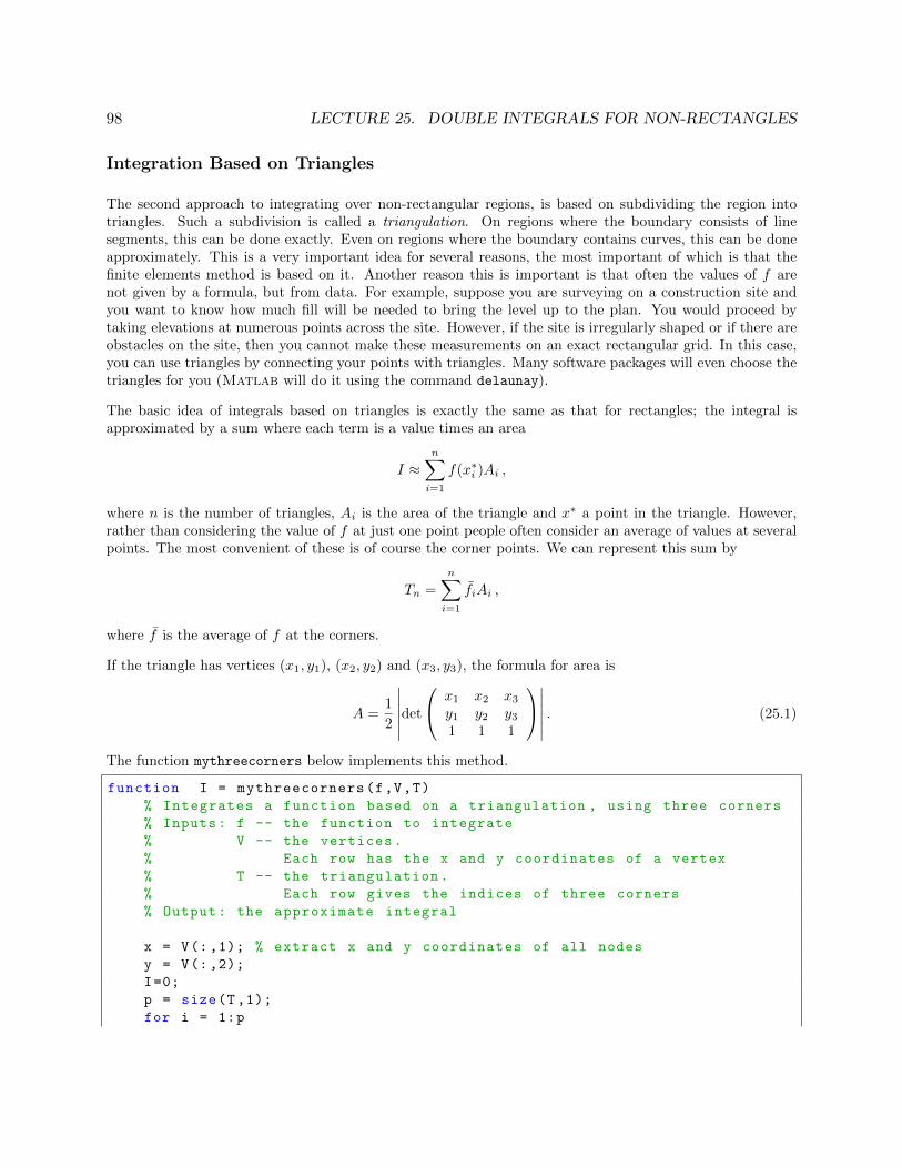
98 LECTURE 25. DOUBLE INTEGRALS FOR NON-RECTANGLES
Integration Based on Triangles
The second approach to integrating over non-rectangular regions, is based on subdividing the region intotriangles. Such a subdivision is called a triangulation. On regions where the boundary consists of linesegments, this can be done exactly. Even on regions where the boundary contains curves, this can be doneapproximately. This is a very important idea for several reasons, the most important of which is that thefinite elements method is based on it. Another reason this is important is that often the values of f arenot given by a formula, but from data. For example, suppose you are surveying on a construction site andyou want to know how much fill will be needed to bring the level up to the plan. You would proceed bytaking elevations at numerous points across the site. However, if the site is irregularly shaped or if there areobstacles on the site, then you cannot make these measurements on an exact rectangular grid. In this case,you can use triangles by connecting your points with triangles. Many software packages will even choose thetriangles for you (Matlab will do it using the command delaunay).
The basic idea of integrals based on triangles is exactly the same as that for rectangles; the integral isapproximated by a sum where each term is a value times an area
I ≈n∑i=1
f(x∗i )Ai ,
where n is the number of triangles, Ai is the area of the triangle and x∗ a point in the triangle. However,rather than considering the value of f at just one point people often consider an average of values at severalpoints. The most convenient of these is of course the corner points. We can represent this sum by
Tn =
n∑i=1
fiAi ,
where f is the average of f at the corners.
If the triangle has vertices (x1, y1), (x2, y2) and (x3, y3), the formula for area is
A =1
2
∣∣∣∣∣∣det
x1 x2 x3y1 y2 y31 1 1
∣∣∣∣∣∣ . (25.1)
The function mythreecorners below implements this method.
function I = mythreecorners(f,V,T)
% Integrates a function based on a triangulation , using three corners
% Inputs: f -- the function to integrate
% V -- the vertices.
% Each row has the x and y coordinates of a vertex
% T -- the triangulation.
% Each row gives the indices of three corners
% Output: the approximate integral
x = V(: ,1); % extract x and y coordinates of all nodes
y = V(: ,2);
I=0;
p = size(T,1);
for i = 1:p

99
x1 = x(T(i,1)); % find coordinates and area
x2 = x(T(i,2));
x3 = x(T(i,3));
y1 = y(T(i,1));
y2 = y(T(i,2));
y3 = y(T(i,3));
A = .5*abs(det([x1, x2, x3; y1, y2, y3; 1, 1, 1]));
z1 = f(x1,y1); % find values and average
z2 = f(x2,y2);
z3 = f(x3,y3);
zavg = (z1 + z2 + z3)/3;
I = I + zavg*A; % accumulate integral
end
end
Another idea would be to use the center point (centroid) of each triangle. If the triangle has vertices (x1, y1),(x2, y2) and (x3, y3), then the centroid is given by the simple formulas
x =x1 + x2 + x3
3and y =
y1 + y2 + y33
. (25.2)
Exercises
25.1 Download the programs mywedge.m and mywasher.m from the web site. Plot f(x, y) = x+yx2+y2 on the
region produced by mywasher.m and f(x, y) = sin(x) +√y on the region produced by mywedge.m.
25.2 Modify the program mythreecorners.m to a new program mycenters.m that does the centerpointmethod for triangles. Run the program on the region produced by mywasher.m with the functionf(x, y) = x+y
x2+y2 and on the region produced by mywedge.m with the function f(x, y) = sin(x) +√y.

Lecture 26
Gaussian Quadrature*
Exercises
26.1
26.2
100

Lecture 27
Numerical Differentiation
Approximating derivatives from data
Suppose that a variable y depends on another variable x, i.e. y = f(x), but we only know the values of f ata finite set of points, e.g., as data from an experiment or a simulation:
(x1, y1), (x2, y2), . . . , (xn, yn).
Suppose then that we need information about the derivative of f(x). One obvious idea would be to approx-imate f ′(xi) by the Forward Difference
f ′(xi) = y′i ≈yi+1 − yixi+1 − xi
.
This formula follows directly from the definition of the derivative in calculus. An alternative would be touse a Backward Difference
f ′(xi) ≈yi − yi−1xi − xi−1
.
Since the errors for the forward difference and backward difference tend to have opposite signs, it wouldseem likely that averaging the two methods would give a better result than either alone. If the points areevenly spaced, i.e. xi+1 − xi = xi − xi−1 = h, then averaging the forward and backward differences leads toa symmetric expression called the Central Difference
f ′(xi) = y′i ≈yi+1 − yi−1
2h.
Errors of approximation
We can use Taylor polynomials to derive the accuracy of the forward, backward and central differenceformulas. For example the usual form of the Taylor polynomial with remainder (sometimes called Taylor’sTheorem) is
f(x+ h) = f(x) + hf ′(x) +h2
2f ′′(c) ,
where c is some (unknown) number between x and x+h. Letting x = xi, x+h = xi+1 and solving for f ′(xi)leads to
f ′(xi) =f(xi+1)− f(xi)
h− h
2f ′′(c).
101

102 LECTURE 27. NUMERICAL DIFFERENTIATION
−0.2 0 0.2 0.4 0.6 0.8 1 1.2−0.2
0
0.2
0.4
0.6
0.8
1
x
y
backward differenceforward differencecentral difference
(xi,y
i)
(xi −1
,yi −1
)
(xi+1
,yi+1
)
Figure 27.1: The three difference approximations of y′i.
Notice that the quotient in this equation is exactly the forward difference formula. Thus the error of theforward difference is −(h/2)f ′′(c) which means it is O(h). Replacing h in the above calculation by −h givesthe error for the backward difference formula; it is also O(h). For the central difference, the error can befound from the third degree Taylor polynomials with remainder
f(xi+1) = f(xi + h) = f(xi) + hf ′(xi) +h2
2f ′′(xi) +
h3
3!f ′′′(c1) and
f(xi−1) = f(xi − h) = f(xi)− hf ′(xi) +h2
2f ′′(xi)−
h3
3!f ′′′(c2) ,
where xi ≤ c1 ≤ xi+1 and xi−1 ≤ c2 ≤ xi. Subtracting these two equations and solving for f ′(xi) leads to
f ′(xi) =f(xi+1)− f(xi−1)
2h− h2
3!
f ′′′(c1) + f ′′′(c2)
2.
This shows that the error for the central difference formula is O(h2). Thus, central differences are significantlybetter and so: It is best to use central differences whenever possible.
There are also central difference formulas for higher order derivatives. These all have error of order O(h2):
f ′′(xi) = y′′i ≈yi+1 − 2yi + yi−1
h2,
f ′′′(xi) = y′′′i ≈1
2h3[yi+2 − 2yi+1 + 2yi−1 − yi−2] , and
f (4)(xi) = y(4)i ≈ 1
h4[yi+2 − 4yi+1 + 6yi − 4yi−1 + yi−2] .
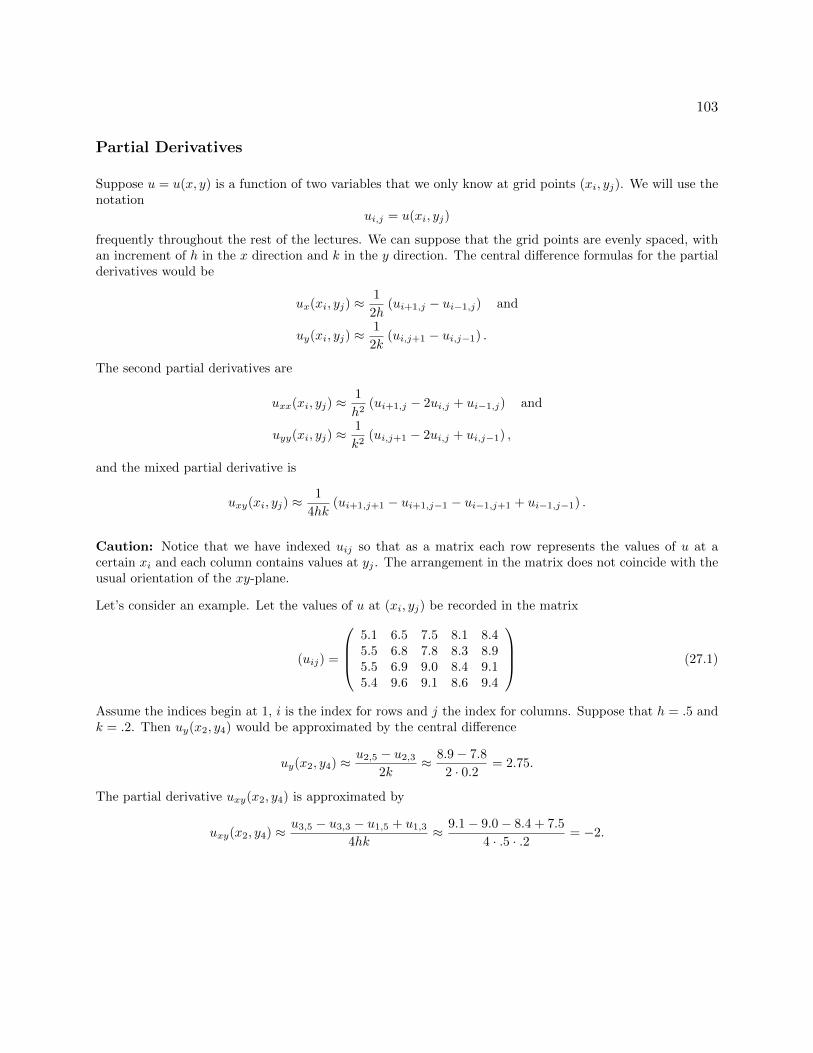
103
Partial Derivatives
Suppose u = u(x, y) is a function of two variables that we only know at grid points (xi, yj). We will use thenotation
ui,j = u(xi, yj)
frequently throughout the rest of the lectures. We can suppose that the grid points are evenly spaced, withan increment of h in the x direction and k in the y direction. The central difference formulas for the partialderivatives would be
ux(xi, yj) ≈1
2h(ui+1,j − ui−1,j) and
uy(xi, yj) ≈1
2k(ui,j+1 − ui,j−1) .
The second partial derivatives are
uxx(xi, yj) ≈1
h2(ui+1,j − 2ui,j + ui−1,j) and
uyy(xi, yj) ≈1
k2(ui,j+1 − 2ui,j + ui,j−1) ,
and the mixed partial derivative is
uxy(xi, yj) ≈1
4hk(ui+1,j+1 − ui+1,j−1 − ui−1,j+1 + ui−1,j−1) .
Caution: Notice that we have indexed uij so that as a matrix each row represents the values of u at acertain xi and each column contains values at yj . The arrangement in the matrix does not coincide with theusual orientation of the xy-plane.
Let’s consider an example. Let the values of u at (xi, yj) be recorded in the matrix
(uij) =
5.1 6.5 7.5 8.1 8.45.5 6.8 7.8 8.3 8.95.5 6.9 9.0 8.4 9.15.4 9.6 9.1 8.6 9.4
(27.1)
Assume the indices begin at 1, i is the index for rows and j the index for columns. Suppose that h = .5 andk = .2. Then uy(x2, y4) would be approximated by the central difference
uy(x2, y4) ≈ u2,5 − u2,32k
≈ 8.9− 7.8
2 · 0.2= 2.75.
The partial derivative uxy(x2, y4) is approximated by
uxy(x2, y4) ≈ u3,5 − u3,3 − u1,5 + u1,34hk
≈ 9.1− 9.0− 8.4 + 7.5
4 · .5 · .2= −2.

104 LECTURE 27. NUMERICAL DIFFERENTIATION
Exercises
27.1 Suppose you are given the data in the following table.t 0 .5 1.0 1.5 2.0y 0 .19 .26 .29 .31
a. Give the forward, backward and central difference approximations of f ′(1).b. Give the central difference approximations for f ′′(1), f ′′′(1) and f (4)(1).
27.2 Suppose values of u(x, y) at points (xi, yj) are given in the matrix (27.1). Suppose that h = .1 andk = .5. Approximate the following derivatives by central differences:a. ux(x2, y4)b. uxx(x3, y2)c. uyy(x3, y2)d. uxy(x2, y3)
Lecture 28
The Main Sources of Error
Truncation Error
Truncation error is defined as the error caused directly by an approximation method. For instance, allnumerical integration methods are approximations and so there is error, even if the calculations are performedexactly. Numerical differentiation also has a truncation error, as will the differential equations methods wewill study in Part IV, which are based on numerical differentiation formulas. There are two ways to minimizetruncation error: (1) use a higher order method, and (2) use a finer grid so that points are closer together.Unless the grid is very small, truncation errors are usually much larger than roundoff errors. The obvioustradeoff is that a smaller grid requires more calculations, which in turn produces more roundoff errors andrequires more running time.
Roundoff Error
Roundoff error always occurs when a finite number of digits are recorded after an operation. Fortunately,this error is extremely small. The standard measure of how small is called machine epsilon. It is definedas the smallest number that can be added to 1 to produce another number on the machine, i.e. if a smallernumber is added the result will be rounded down to 1. In IEEE standard double precision (used by Matlaband most serious software), machine epsilon is 2−52 or about 2.2× 10⁻¹⁶. A different, but equivalent, way ofthinking about this is that the machine records 52 floating binary digits or about 15 floating decimal digits.Thus there are never more than 15 significant digits in any calculation. This of course is more than adequatefor any application. However, there are ways in which this very small error can cause problems.
To see an unexpected occurence of round-off try
(2^52+1) - 2^52
(2^53+1) - 2^53
Loss of Precision (also called Loss of Significance)
One way in which small roundoff errors can become more significant is when significant digits cancel. Forinstance, if you were to calculate
1234567(1− .9999987654321)
then the result should be1.52415678859930 ,
105

106 LECTURE 28. THE MAIN SOURCES OF ERROR
which has 15 significant digits. But if you input
1234567 * ( 1 - .9999987654321)
you will get 1.52415678862573, which has only 11 significant digits even though Matlab used 15 digitsin all its calculations. The problem is that the subtraction 1 − .9999987654321 converts significant digitsto leading zeros, which are not significant digits. Multiplication by 1234567 does not cause any loss ofsiginficance, but hides the problem by making us think we have a reasonable size number.
Although this seems like a silly example, this type of loss of precision can happen by accident, with catas-trophic results, if you are not careful. For example in f ′(x) ≈ (f(x + h) − f(x))/h you will lose precisionwhen h gets too small. Try
format long
format compact
f = @(x) x^2
for i = 1:30
h = 10^(-i)
df = (f(1+h)-f(1))/h
relerr = (2-df)/2
end
At first the relative error decreases since truncation error is reduced. Then loss of precision takes over andthe relative error increases to 1.
Bad Conditioning
We encountered bad conditioning in Part II, when we talked about solving linear systems. Bad conditioningmeans that the problem is unstable in the sense that small input errors can produce large output errors. Thiscan be a problem in a couple of ways. First, the measurements used to get the inputs cannot be completelyaccurate. Second, the computations along the way have roundoff errors. Errors in the computations nearthe beginning especially can be magnified by a factor close to the condition number of the matrix. Thuswhat was a very small problem with roundoff can become a very big problem.
It turns out that matrix equations are not the only place where condition numbers occur. In any problemone can define the condition number as the maximum ratio of the relative errors in the output versus input,i.e.
condition # of a problem = max
(Relative error of output
Relative error of inputs
).
An easy example is solving a simple equation
f(x) = 0.
Suppose that f ′ is close to zero at the solution x∗. Then a very small change in f (caused perhaps by aninaccurate measurement of some of the coefficients in f) can cause a large change in x∗. It can be shownthat the condition number of this problem is 1/f ′(x∗).

107
Exercises
28.1 Identify the (main) source of error in each case and propose a way to reduce this error if possible.
(a) If we do (√
3)2 we should get 3, but if we check
mythree = (sqrt (3))^2
mythree -3
we find the error is ans = -4.4409e-16.
(b) Since it is a quarter of a circle of radius 2, we should have∫ 2
0
√4− x2dx = 1
4π22 = π. We try touse mytrap from Lecture 21 and do
x = 0:.2:2;
y = sqrt(4-x.^2);
mypi = mytrap(x,y)
mypi -pi
and find the error is ans = -0.0371.
28.2 1 The function f(x) = (x−2)9 could be evaluated as written, or first expanded as f(x) = x9−18x8+· · ·and then evaluated. To find the expanded version, type
syms x
expand ((x -2)^9)
clear
To evaluate it the first way, type
f1 = @(x) (x -2).^9
x = 1.92:.001:2.08;
y1 = f1(x);
plot(x,y1,’blue’)
To do it the second way, convert the expansion above to an anonymous function f2 and then type
y2 = f2(x);
hold on
plot(x,y2,’red’)
Carefully study the resulting graphs. Should the graphs be the same? Which is more correct? Matlabdoes calculations using approximately 16 decimal places. What is the largest error in the graph, andhow big is it relative to 10−16? Which source of error is causing this problem?
1From Numerical Linear Algebra by L. Trefethen and D. Bau, SIAM, 1997.

Review of Part III
Methods and Formulas
Polynomial Interpolation:
An exact fit to the data.For n data points it is a n− 1 degree polynomial.Only good for very few, accurate data points.The coefficients are found by solving a linear system of equations.
Spline Interpolation:
Fit a simple function between each pair of points.Joining points by line segments is the most simple spline.Cubic is by far the most common and important.Cubic matches derivatives and second derivatives at data points.Simply supported and clamped ends are available.Good for more, but accurate points.The coefficients are found by solving a linear system of equations.
Least Squares:
Makes a “close fit” of a simple function to all the data.Minimizes the sum of the squares of the errors.Good for noisy data.The coefficients are found by solving a linear system of equations.
Interpolation vs. Extrapolation:
Polynomials, Splines and Least Squares are generally used for Interpolation, fitting between the data. Ex-trapolation, i.e. making fits beyond the data, is much more tricky. To make predictions beyond the data,you must have knowledge of the underlying process, i.e. what the function should be.
108

109
Numerical Integration:
Left Endpoint:
Ln =
n∑i=1
f(xi−1)∆xi
Right Endpoint:
Rn =
n∑i=1
f(xi)∆xi.
Trapezoid Rule:
Tn =
n∑i=1
f(xi−1) + f(xi)
2∆xi.
Midpoint Rule:
Mn =
n∑i=1
f(xi)∆xi where xi =xi−1 + xi
2.
Numerical Integration Rules with Even Spacing:
For even spacing: ∆x = b−an where n is the number of subintervals, then:
Ln = ∆x
n−1∑i=0
yi =b− an
n−1∑i=0
f(xi),
Rn = ∆x
n∑i=1
yi =b− an
n∑i=1
f(xi),
Tn = ∆x(y0 + 2y1 + . . .+ 2yn−1 + yn
)=b− a2n
(f(x0) + 2f(x1) + . . .+ 2f(xn−1) + f(xn)
),
Mn = ∆x
n∑i=1
yi =b− an
n∑i=1
f(xi),
Simpson’s rule:
Sn = ∆x(y0 + 4y1 + 2y2 + 4y3 + . . .+ 2yn−2 + 4yn−1 + yn
)=b− a3n
(f(x0) + 4f(x1) + 2f(x2) + 4f(x3) + . . .+ 2f(xn−2) + 4f(xn−1) + f(xn)) .
Area of a region:
A = −∮C
y dx,
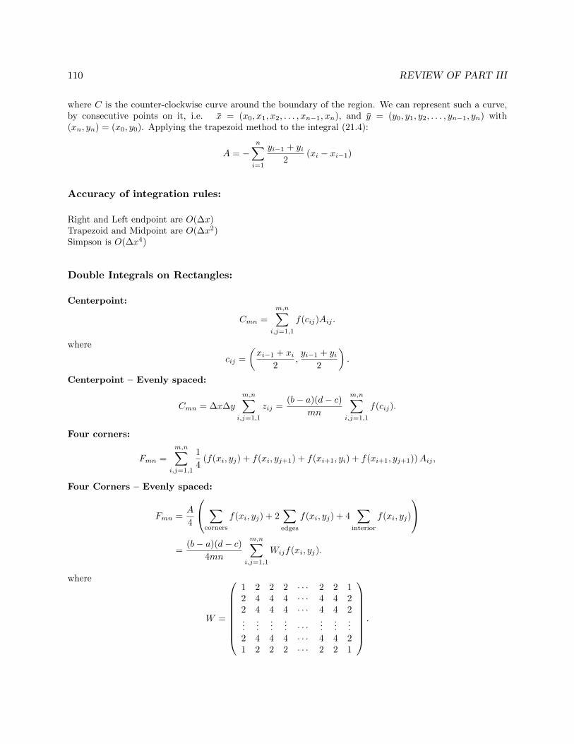
110 REVIEW OF PART III
where C is the counter-clockwise curve around the boundary of the region. We can represent such a curve,by consecutive points on it, i.e. x = (x0, x1, x2, . . . , xn−1, xn), and y = (y0, y1, y2, . . . , yn−1, yn) with(xn, yn) = (x0, y0). Applying the trapezoid method to the integral (21.4):
A = −n∑i=1
yi−1 + yi2
(xi − xi−1)
Accuracy of integration rules:
Right and Left endpoint are O(∆x)Trapezoid and Midpoint are O(∆x2)Simpson is O(∆x4)
Double Integrals on Rectangles:
Centerpoint:
Cmn =
m,n∑i,j=1,1
f(cij)Aij .
where
cij =
(xi−1 + xi
2,yi−1 + yi
2
).
Centerpoint – Evenly spaced:
Cmn = ∆x∆y
m,n∑i,j=1,1
zij =(b− a)(d− c)
mn
m,n∑i,j=1,1
f(cij).
Four corners:
Fmn =
m,n∑i,j=1,1
1
4(f(xi, yj) + f(xi, yj+1) + f(xi+1, yi) + f(xi+1, yj+1))Aij ,
Four Corners – Evenly spaced:
Fmn =A
4
∑corners
f(xi, yj) + 2∑edges
f(xi, yj) + 4∑
interior
f(xi, yj)
=
(b− a)(d− c)4mn
m,n∑i,j=1,1
Wijf(xi, yj).
where
W =
1 2 2 2 · · · 2 2 12 4 4 4 · · · 4 4 22 4 4 4 · · · 4 4 2...
......
... · · ·...
......
2 4 4 4 · · · 4 4 21 2 2 2 · · · 2 2 1
.

111
Double Simpson:
Smn =(b− a)(d− c)
9mn
m,n∑i,j=1,1
Wijf(xi, yj).
where
W =
1 4 2 4 · · · 2 4 14 16 8 16 · · · 8 16 42 8 4 8 · · · 4 8 24 16 8 16 · · · 8 16 4...
......
... · · ·...
......
2 8 4 8 · · · 4 8 24 16 8 16 · · · 8 16 41 4 2 4 · · · 2 4 1
.
Integration based on triangles:
– Triangulation: Dividing a region up into triangles.– Triangles are suitable for odd-shaped regions.– A triangulation is better if the triangles are nearly equilateral.Three corners:
Tn =
n∑i=1
fiAi
where f is the average of f at the corners of the i-th triangle.Area of a triangle with corners (x1, y1), (x2, y2), (x3, y3):
A =1
2
∣∣∣∣∣∣det
x1 x2 x3y1 y2 y31 1 1
∣∣∣∣∣∣ .Centerpoint:
C =
n∑i=1
f(xi, yi)Ai, with
x =x1 + x2 + x3
3and y =
y1 + y2 + y33
.
Finite Differences
Forward Difference:
f ′(xi) = y′i ≈yi+1 − yixi+1 − xi
.
Backward Difference:
f ′(xi) ≈yi − yi−1xi − xi−1
.
Central Difference:
f ′(xi) = y′i ≈yi+1 − yi−1
2h.
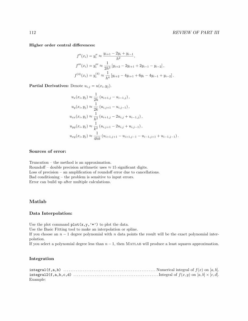
112 REVIEW OF PART III
Higher order central differences:
f ′′(xi) = y′′i ≈yi+1 − 2yi + yi−1
h2,
f ′′′(xi) = y′′′i ≈1
2h3[yi+2 − 2yi+1 + 2yi−1 − yi−2] ,
f (4)(xi) = y(4)i ≈ 1
h4[yi+2 − 4yi+1 + 6yi − 4yi−1 + yi−2] .
Partial Derivatives: Denote ui,j = u(xi, yj).
ux(xi, yj) ≈1
2h(ui+1,j − ui−1,j) ,
uy(xi, yj) ≈1
2k(ui,j+1 − ui,j−1) ,
uxx(xi, yj) ≈1
h2(ui+1,j − 2ui,j + ui−1,j) ,
uyy(xi, yj) ≈1
k2(ui,j+1 − 2ui,j + ui,j−1) ,
uxy(xi, yj) ≈1
4hk(ui+1,j+1 − ui+1,j−1 − ui−1,j+1 + ui−1,j−1) .
Sources of error:
Truncation – the method is an approximation.Roundoff – double precision arithmetic uses ≈ 15 significant digits.Loss of precision – an amplification of roundoff error due to cancellations.Bad conditioning – the problem is sensitive to input errors.Error can build up after multiple calculations.
Matlab
Data Interpolation:
Use the plot command plot(x,y,’*’) to plot the data.Use the Basic Fitting tool to make an interpolation or spline.If you choose an n − 1 degree polynomial with n data points the result will be the exact polynomial inter-polation.If you select a polynomial degree less than n− 1, then Matlab will produce a least squares approximation.
Integration
integral(f,a,b) . . . . . . . . . . . . . . . . . . . . . . . . . . . . . . . . . . . . . . . . . . . . . . . . . . . . Numerical integral of f(x) on [a, b].integral2(f,a,b,c,d) . . . . . . . . . . . . . . . . . . . . . . . . . . . . . . . . . . . . . . . . . . . . . . . . Integral of f(x, y) on [a, b]× [c, d].Example:

113
f = @(x,y) sin(x.*y)/sqrt(x+y)
I = integral2(f,0,1,0,2)
Matlab uses an advanced form of Simpson’s method.
Integration over non-rectangles:
Redefine the function to be zero outside the region. For example:
f = @(x,y) sin(x.*y).^3.*(2*x + y <= 2)
I = integral2(f,0,1,0,2)
Integrates f(x, y) = sin3(xy) on the triangle with corners (0, 0), (0, 2), and (1, 0).
Triangles:Matlab stores triangulations as a matrix of vertices V and triangles T.T = delaunay(V) (or delaunay(x,y)) . . . . . . . . . . . . . . . . . . . . . . . . . . . . . . . . . Produces triangles from vertices.trimesh(T,x,y)
trimesh(T,x,y,z)
trisurf(T,x,y)
trisurf(T,x,y,z)
Logical expressions
(2*x + y <= 2), (x.^2+y.^2<=1) are examples of logical expressions.If a logical expression is true it is given the value 1. If false, then it is assigned the value 0.

114 REVIEW OF PART III

Part IV
Differential Equations
c©Copyright, Todd Young and Martin Mohlenkamp, Department of Mathematics, Ohio University, 2017

Lecture 29
Reduction of Higher Order Equations toSystems
The motion of a pendulum
Consider the motion of an ideal pendulum that consists of a mass m attached to an arm of length `. If weignore friction, then Newton’s laws of motion tell us
mθ = −mg`
sin θ,
where θ is the angle of displacement. tAAAAAAAAw`θ
Figure 29.1: A pendulum.
If we also incorporate moving friction and sinusoidal forcing then the equation takes the form
mθ + γθ +mg
`sin θ = A sin Ωt.
Here γ is the coefficient of friction and A and Ω are the amplitude and frequency of the forcing. Usually,this equation would be rewritten by dividing through by m to produce
θ + cθ + ω sin θ = a sin Ωt, (29.1)
where c = γ/m. ω = g/` and a = A/m.
This is a second order ODE because the second derivative with respect to time t is the highest derivative. Itis nonlinear because it has the term sin θ and which is a nonlinear function of the dependent variable θ. A
116
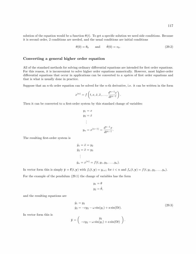
117
solution of the equation would be a function θ(t). To get a specific solution we need side conditions. Becauseit is second order, 2 conditions are needed, and the usual conditions are initial conditions
θ(0) = θ0 and θ(0) = v0. (29.2)
Converting a general higher order equation
All of the standard methods for solving ordinary differential equations are intended for first order equations.For this reason, it is inconvenient to solve higher order equations numerically. However, most higher-orderdifferential equations that occur in applications can be converted to a system of first order equations andthat is what is usually done in practice.
Suppose that an n-th order equation can be solved for the n-th derivative, i.e. it can be written in the form
x(n) = f
(t, x, x, x, . . . ,
dn−1x
dtn−1
).
Then it can be converted to a first-order system by this standard change of variables:
y1 = x
y2 = x
...
yn = x(n−1) =dn−1x
dtn−1.
The resulting first-order system is
y1 = x = y2
y2 = x = y3
...
yn = x(n) = f(t, y1, y2, . . . , yn).
In vector form this is simply y = f(t,y) with fi(t,y) = yi+1 for i < n and fn(t,y) = f(t, y1, y2, . . . , yn).
For the example of the pendulum (29.1) the change of variables has the form
y1 = θ
y2 = θ,
and the resulting equations are
y1 = y2
y2 = −cy2 − ω sin(y1) + a sin(Ωt).(29.3)
In vector form this is
y =
(y2
−cy2 − ω sin(y1) + a sin(Ωt)
).
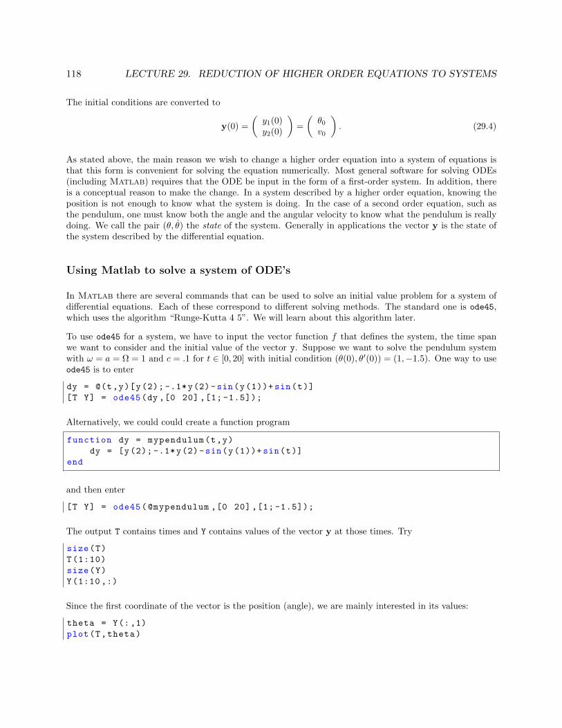
118 LECTURE 29. REDUCTION OF HIGHER ORDER EQUATIONS TO SYSTEMS
The initial conditions are converted to
y(0) =
(y1(0)y2(0)
)=
(θ0v0
). (29.4)
As stated above, the main reason we wish to change a higher order equation into a system of equations isthat this form is convenient for solving the equation numerically. Most general software for solving ODEs(including Matlab) requires that the ODE be input in the form of a first-order system. In addition, thereis a conceptual reason to make the change. In a system described by a higher order equation, knowing theposition is not enough to know what the system is doing. In the case of a second order equation, such asthe pendulum, one must know both the angle and the angular velocity to know what the pendulum is reallydoing. We call the pair (θ, θ) the state of the system. Generally in applications the vector y is the state ofthe system described by the differential equation.
Using Matlab to solve a system of ODE’s
In Matlab there are several commands that can be used to solve an initial value problem for a system ofdifferential equations. Each of these correspond to different solving methods. The standard one is ode45,which uses the algorithm “Runge-Kutta 4 5”. We will learn about this algorithm later.
To use ode45 for a system, we have to input the vector function f that defines the system, the time spanwe want to consider and the initial value of the vector y. Suppose we want to solve the pendulum systemwith ω = a = Ω = 1 and c = .1 for t ∈ [0, 20] with initial condition (θ(0), θ′(0)) = (1,−1.5). One way to useode45 is to enter
dy = @(t,y)[y(2); -.1*y(2)-sin(y(1))+ sin(t)]
[T Y] = ode45(dy ,[0 20] ,[1; -1.5]);
Alternatively, we could could create a function program
function dy = mypendulum(t,y)
dy = [y(2); -.1*y(2)-sin(y(1))+ sin(t)]
end
and then enter
[T Y] = ode45(@mypendulum ,[0 20] ,[1; -1.5]);
The output T contains times and Y contains values of the vector y at those times. Try
size(T)
T(1:10)
size(Y)
Y(1:10 ,:)
Since the first coordinate of the vector is the position (angle), we are mainly interested in its values:
theta = Y(:,1)
plot(T,theta)
119
In the next two sections we will learn enough about numerical methods for initial value problems to under-stand roughly how Matlab produces this approximate solution.
Exercises
29.1 Consider the pendulum system but with no friction or forcing, i.e. γ = A = 0. What would equation(29.3) become in this case? Use the last example to solve the system with the initial condition [θ0, 0]′
for θ0 = .1π. Use the plot of the solution to find the frequency of the pendulum with this initialcondition. Do the same for θ0 = .5π and .9π. How does the frequency depend on the amplitude of apendulum?
29.2 Transform the ODE...x + x2 − 3x3 + cos2 x = e−t sin(3t)
into a first order system. Suppose the initial conditions for the ODE are x(1) = 1, x(1) = 2, andx(1) = 0. Find a numerical solution of this IVP using ode45 and plot the first coordinate (x). Try timeintervals [1 2] and [1 2.1] and explain what you observe. (Remember to use entry-wise operations,.* and .^, in the definition of the vector function.)

Lecture 30
Euler Methods
Numerical Solution of an IVP
Suppose we wish to numerically solve the initial value problem
y = f(t,y), y(a) = y0, (30.1)
on an interval of time [a, b].
By a numerical solution, we must mean an approximation of the solution at a finite number of points, i.e.
(t0,y0), (t1,y1), (t2,y2), . . . , (tn,yn),
where t0 = a and tn = b. The first of these points is exactly the initial value. If we take n steps as above,and the steps are evenly spaced, then the time change in each step is
h =b− an
, (30.2)
and the times ti are given simply by ti = a+ ih. This leaves the most important part of finding a numericalsolution: determining y1,y2, . . . ,yn in a way that is as consistent as possible with (30.1). To do this, firstwrite the differential equation in the indexed notation
yi ≈ f(ti,yi), (30.3)
and then replace the derivative y by a difference. There are many ways we might carry this out and in thenext section we study the simplest.
The Euler Method
The most straight forward approach is to replace yi in (30.3) by its forward difference approximation. Thisgives
yi+1 − yih
= f(ti,yi).
Rearranging this gives us a way to obtain yi+1 from yi known as Euler’s method:
yi+1 = yi + hf(ti,yi). (30.4)
With this formula, we can start from (t0,y0) and compute all the subsequent approximations (ti,yi). Thisis very easy to implement, as you can see from the following program (which can be downloaded from theclass web site).
120

121
function [T , Y] = myeuler(f,tspan ,y0,n)
% function [T , Y] = myeuler(f,tspan ,y0,n)
% Solves dy/dt = f(t,y) with initial condition y(a) = y0
% on the interval [a,b] using n steps of Euler s method.
% Inputs: f -- a function f(t,y) that returns a column vector of the
% same length as y
% tspan -- a vector [a,b] with the start and end times
% y0 -- a column vector of the initial values , y(a) = y0
% n -- number of steps to use
% Outputs: T -- a n+1 column vector containing the times
% Y -- a (n+1) by d matrix where d is the length of y
% Y(j,i) gives the ith component of y at time T(j)
a = tspan (1); b = tspan (2); % parse starting and ending points
h = (b-a)/n; % step size
t = a; T = a; % t is the current time and T will record all times
y = y0; % y is the current variable values , as a column vector
Y = y0 ’; % Y will record the values at all steps , each in a row
for i = 1:n
y = y + h*f(t,y); % Euler update of y to next time
t = a + i*h; % The next time.
T = [T; t]; % Record t and y into T and Y.
Y = [Y; y’];
end
end
To use this program we need a function, such as the vector function for the pendulum:
dy = @(t,y)[y(2); -.1*y(2)-sin(y(1))+ sin(t)]
Save this and then type
[T Y] = myeuler(dy ,[0 20] ,[1; -1.5] ,5);
Here [0 20] is the time span you want to consider, [1;-1.5] is the initial value of the vector y and 5 is thenumber of steps. The output T contains times and Y contains values of the vector as the times. Try
size(T)
size(Y)
Since the first coordinate of the vector is the angle, we only plot its values:
theta = Y(:,1);
plot(T,theta)
In this plot it is clear that n = 5 is not adequate to represent the function. Type
hold on
122 LECTURE 30. EULER METHODS
then redo the above with 5 replaced by 10. Next try 20, 40, 80, and 200. As you can see the graph becomesincreasingly better as n increases. We can compare these calculations with Matlab’s built-in function withthe commands
[T Y]= ode45(dy ,[0 20] ,[1; -1.5]);
theta = Y(:,1);
plot(T,theta ,’r’)
The problem with the Euler method
You can think of the Euler method as finding a linear approximate solution to the initial value problem oneach time interval. An obvious shortcoming of the method is that it makes the approximation based oninformation at the beginning of the time interval only. This problem is illustrated well by the following IVP:
x+ x = 0 with x(0) = 1 and x(0) = 0 . (30.5)
You can easily check that the exact solution of this IVP is
x(t) = cos(t).
If we make the standard change of variables
y1 = x and y2 = x,
then we gety1 = y2 and y2 = −y1.
Then the solution should be y1(t) = cos(t) and y2(t) = sin(t). If we then plot the solution in the (y1, y2)plane, we should get exactly a unit circle. We can solve this IVP with Euler’s method:
dy = @(t,y)[y(2);-y(1)]
[T Y] = myeuler(dy ,[0 4*pi] ,[1;0] ,20)
y1 = Y(:,1);
y2 = Y(:,2);
plot(y1 ,y2)
As you can see the approximate solution goes far from the true solution. Even if you increase the numberof steps, the Euler solution will eventually drift outward away from the circle because it does not take intoaccount the curvature of the solution.
The Modified Euler Method
An idea which is similar to the idea behind the trapezoid method would be to consider f at both thebeginning and end of the time step and take the average of the two. Doing this produces the Modified (orImproved) Euler method represented by the following equations:
k1 = hf(ti,yi)
k2 = hf(ti + h,yi + k1)
yi+1 = yi +1
2(k1 + k2) .
(30.6)
123
Here k1 captures the information at the beginning of the time step (same as Euler), while k2 is the informationat the end of the time step.
A program mymodeuler.m that implements the Modified method may be downloaded from the class website.
Test this program on the IVP above:
[T Ym] = mymodeuler(dy ,[0 4*pi] ,[1;0] ,20)
ym1 = Ym(:,1);
ym2 = Ym(:,2);
plot(ym1 ,ym2)
You will find that the results are much better than for the plain Euler method.
Exercises
30.1 Download the files myeuler.m and mymodeuler.m from the class web site.
(a) Type the following commands:
dy = @(t,y) sin(t)*cos(y);
hold on
[T Y] = myeuler(dy ,[0 ,12] ,.1 ,20);
plot(T,Y)
Position the plot window so that it can always be seen and type
[T Y] = myeuler(dy ,[0 ,12] ,.1 ,30);
plot(T,Y)
(You can use the up button to reduce typing.) Continue to increase the last number in the aboveuntil the graph stops changing (as far as you can see). Record this number and print the finalgraph. Type hold off and kill the plot window.
(b) Follow the same procedure using mymodeuler.m .
(c) Describe what you observed. In particular compare how fast the two methods converge as n isincreased (h is decreased).
Lecture 31
Higher Order Methods
The order of a method
For numerical solutions of an initial value problem there are two ways to measure the error. The first is theerror of each step. This is called the Local Truncation Error or LTE. The other is the total error for thewhole interval [a, b]. We call this the Global Truncation Error or GTE.
For the Euler method the LTE is of order O(h2), i.e. the error is comparable to h2. We can show this directlyusing Taylor’s Theorem:
y(t+ h) = y(t) + hy(t) +h2
2y(c)
for some c between t and t+ h. In this equation we can replace y(t) by f(t,y(t)), which makes the first two
terms of the right hand side be exactly the Euler method. The error is then h2
2 y(c) or O(h2). It would beslightly more difficult to show that the LTE of the modified Euler method is O(h3), an improvement of onepower of h.
We can roughly get the GTE from the LTE by considering the number of steps times the LTE. For anymethod, if [a, b] is the interval and h is the step size, then n = (b−a)/h is the number of steps. Thus for anymethod, the GTE is one power lower in h than the LTE. Thus the GTE for Euler is O(h) and for modifiedEuler it is O(h2).
By the order of a method, we mean the power of h in the GTE. Thus the Euler method is a 1st ordermethod and modified Euler is a 2nd order method.
Fourth Order Runge-Kutta
The most famous of all IVP methods is the classic Runge-Kutta method of order 4:
k1 = hf(ti,y)
k2 = hf(ti + h/2,yi + k1/2)
k3 = hf(ti + h/2,yi + k2/2)
k4 = hf(ti + h,yi + k3)
yi+1 = yi +1
6(k1 + 2k2 + 2k3 + k4) .
(31.1)
Notice that this method uses values of f(t,y) at 4 different points. In general a method needs n values of f toachieve order n. The constants used in this method and other methods are obtained from Taylor’s Theorem.
124
125
They are precisely the values needed to make all error terms cancel up to hn+1f (n+1)(c)/(n+ 1)!.
Variable Step Size and RK45
If the order of a method is n, then the GTE is comparable to hn, which means it is approximately Chn,where C is some constant. However, for different differential equations, the values of C may be very different.Thus it is not easy beforehand to tell how small h should be to get the error within a given tolerence. Forinstance, if the true solution oscillates very rapidly, we will obviously need a smaller step size than for asolution that is nearly constant.
How can a program then choose h small enough to produce the required accuracy? We also do not wish tomake h much smaller than necessary, since that would increase the number of steps. To accomplish this aprogram tries an h and tests to see if that h is small enough. If not it tries again with a smaller h. If it istoo small, it accepts that step, but on the next step it tries a larger h. This process is called variable stepsize.
Deciding if a single step is accurate enough could be accomplished in several ways, but the most commonare called embedded methods. The Runge-Kutta 45 method, which is used in ode45, is an embeddedmethod. In the RK45, the function f is evaluated at 5 different points. These are used to make a 5th orderestimate yi+1. At the same time, 4 of the 5 values are used to also get a 4th order estimate. If the 4thorder and 5th order estimates are close, then we can conclude that they are accurate. If there is a largediscrepency, then we can conclude that they are not accurate and a smaller h should be used.
To see variable step size in action, we will define and solve two different ODEs and solve them on the sameinterval. Create this script and run it:
dy1 = @(t,y) [-y(2);y(1)];
dy2 = @(t,y) [-5*y(2);5*y(1)];
[T1 Y1] = ode45(dy1 ,[0 20] ,[1;0]);
[T2 Y2] = ode45(dy2 ,[0 20] ,[1;0]);
y1 = Y1(:,1);
y2 = Y2(:,1);
plot(T1 ,y1 ,’bx -’)
hold on
plot(T2 ,y2 ,’ro -’)
size(T1)
size(T2)
Why order matters
Many people would conclude on first encounter that the advantage of a higher order method would be thatyou can get a more accurate answer than for a lower order method. In reality, this is not quite how thingswork. In engineering problems, the accuracy needed is usually a given and it is usually not extremely high.Thus getting more and more accurate solutions is not very useful. So where is the advantage? Consider thefollowing example.
Suppose that you need to solve an IVP with an error of less than 10−4. If you use the Euler method, which

126 LECTURE 31. HIGHER ORDER METHODS
has GTE of order O(h), then you would need h ≈ 10−4. So you would need about n ≈ (b − a) × 104 stepsto find the solution.
Suppose you use the second order, modified Euler method. In that case the GTE is O(h2), so you wouldneed to use h2 ≈ 10−4, or h ≈ 10−2. This would require about n ≈ (b − a) × 102 steps. That is a hundredtimes fewer steps than you would need to get the same accuracy with the Euler method.
If you use the RK4 method, then h4 needs to be approximately 10−4, and so h ≈ 10−1. This means youneed only about n ≈ (b− a)× 10 steps to solve the problem, i.e. a thousand times fewer steps than for theEuler method.
Thus the real advantage of higher order methods is that they can run a lot faster at the same accuracy. Thiscan be especially important in applications where one is trying to make real-time adjustments based on thecalculations. Such is often the case in robots and other applications with dynamic controls.
Exercises
31.1 There is a Runge-Kutta 2 method, which is also known as the midpoint method. It is summarized bythe following equations:
k1 = hf(ti,yi)
k2 = hf(ti + h/2,yi + k1/2)
yi+1 = yi + k2.
(31.2)
(a) Modify the program mymodeuler into a program myRK2 that does the RK2 method.
(b) Test myRK2 and mymodeuler on the following IVP with time span [0, 4π]:
x+ x = 0 with x(0) = 1 and x(0) = 0.
Using format long, make a table with yn+1 for each of the two programs for n = 10, 100, and1000. Compute the difference between yn+1 and the true solution y(4π) = (1, 0).
Turn in the modified program and a summary of the results.

Lecture 32
Multi-step Methods*
Exercises
32.1
127

Lecture 33
ODE Boundary Value Problems and FiniteDifferences
Steady State Heat and Diffusion
If we consider the movement of heat in a long thin object (like a metal bar), it is known that the temperature,u(x, t), at a location x and time t satisfies the partial differential equation
ut − uxx = g(x, t), (33.1)
where g(x, t) is the effect of any external heat source. The same equation also describes the diffusion of achemical in a one-dimensional environment. For example the environment might be a canal, and then g(x, t)would represent how a chemical is introduced.
Sometimes we are interested only in the steady state of the system, supposing g(x, t) = g(x) and u(x, t) =u(x). In this case
uxx = −g(x).
This is a linear second-order ordinary differential equation. We could find its solution exactly if g(x) isnot too complicated. If the environment or object we consider has length L, then typically one would haveconditions on each end of the object, such as u(0) = 0, u(L) = 0. Thus instead of an initial value problem,we have a boundary value problem or BVP.
Beam With Tension
Consider a simply supported beam with modulus of elasticity E, moment of inertia I, a uniform load w,and end tension T (see Figure 33.1). If y(x) denotes the deflection at each point x in the beam, then y(x)satisfies the differential equation
y′′
(1 + (y′)2)3/2− T
EIy =
wx(L− x)
2EI, (33.2)
with boundary conditions y(0) = y(L) = 0. This equation is nonlinear and there is no hope to solve itexactly. If the deflection is small then (y′)2 is negligible compared to 1 and the equation approximatelysimplifies to
y′′ − T
EIy =
wx(L− x)
2EI. (33.3)
This is a linear equation and we can find the exact solution. We can rewrite the equation as
y′′ − αy = βx(L− x), (33.4)
128

129
t t -T T
? ? ? ? ?
w
Figure 33.1: A simply supported beam with a uniform load w and end tension T .
where
α =T
EIand β =
w
2EI, (33.5)
and then the exact solution is
y(x) =2β
α2
e√αL
e√αL + 1
e−√αx +
2β
α2
1
e√αL + 1
e√αx +
β
αx2 − βL
αx+
2β
α2. (33.6)
Finite Difference Method – Linear ODE
A finite difference equation is an equation obtained from a differential equation by replacing the variablesby their discrete versions and derivatives by difference formulas.
First we will consider equation (33.3). Suppose that the beam is a W12x22 structural steel I-beam. ThenL = 120 in., E = 29 × 106lb./in.2 and I = 121in.4. Suppose that the beam is carrying a uniform load of100, 000 lb. so that w = 120, 000/120 = 10, 000 and a tension of T = 10, 000 lb.. We calculate from (33.5)α = 2.850× 10⁻⁶ and β = 1.425× 10⁻⁶. Thus we have the following BVP:
y′′ = 2.850× 10⁻⁶y + 1.425× 10−6x(120− x), y(0) = y(120) = 0. (33.7)
First subdivide the interval [0, 120] into four equal subintervals. The nodes of this subdivion are x0 = 0,x1 = 30, x2 = 60, . . . , x4 = 120. We will then let y0, y1, . . . , y4 denote the deflections at the nodes. Fromthe boundary conditions we have immediately:
y0 = y4 = 0.
To determine the deflections at the interior points we will rely on the differential equation. Recall the centraldifference formula
y′′(xi) ≈yi+1 − 2yi + yi−1
h2.
In this case we have h = (b− a)/n = (120− 0)/4 = 30. Replacing all the variables in the equation (33.4) bytheir discrete versions we get
yi+1 − 2yi + yi−1 = h2αyi + h2βxi(L− xi).
Substituting in for α, β and h we obtain:
yi+1 − 2yi + yi−1 = 900× 2.850× 10−6yi + 900× 1.425× 10−6xi(120− xi)= 2.565× 10⁻³yi + 1.2825× 10⁻³xi(120− xi).

130 LECTURE 33. ODE BOUNDARY VALUE PROBLEMS AND FINITE DIFFERENCES
This equation makes sense for i = 1, 2, 3. At x1 = 30, the equation becomes:
y2 − 2y1 + y0 = 2.565× 10⁻³y1 + 1.2825× 10−3 × 30(90)
⇔ y2 − 2.002565y1 = 3.46275.(33.8)
Note that this equation is linear in the unknowns y1 and y2. At x2 = 60 we have:
y3 − 2y2 + y1 = .002565y2 + 1.2825× 10−3 × 602
⇔ y3 − 2.002565y2 + y1 = 4.617.(33.9)
At x3 = 90 we have (since y4 = 0)
−2.002565y3 + y2 = 3.46275. (33.10)
Thus (y1, y2, y3) is the solution of the linear system: −2.002565 1 0 3.462751 −2.002565 1 4.6170 1 −2.002565 3.46275
.
We can easily find the solution of this system in Matlab:
A = [ -2.002565 1 0 ; 1 -2.002565 1 ; 0 1 -2.002565]
b = [ 3.46275 4.617 3.46275 ]’
y = A\b
To graph the solution, we need define the x values and add on the values at the endpoints:
x = 0:30:120
y = [0 ; y ; 0]
plot(x,y,’d’)
Adding a spline will result in an excellent graph.
The exact solution of this BVP is given in (33.6). That equation, with the parameter values for the W12x22I-beam as in the example, is in the program myexactbeam.m on the web site. We can plot the true solutionon the same graph:
hold on
myexactbeam
Thus our numerical solution is extremely good considering how few subintervals we used and how very largethe deflection is.
An amusing exercise is to set T = 0 in the program myexactbeam.m; the program fails because the exactsolution is no longer valid. Also try T = .1 for which you will observe loss of precision. On the other handthe finite difference method still works when we set T = 0.

131
Exercises
33.1 Derive the finite difference equations for the BVP (33.7) on the same domain ([0, 120]), but with eightsubintervals and solve (using Matlab) as in the example. Plot your result, together on the same plotwith the exact solution (33.6) from the program myexactbeam.m.
33.2 By replacing y′′ and y′ with central differences, derive the finite difference equation for the boundaryvalue problem
y′′ + y′ − y = x on [0, 1] with y(0) = y(1) = 0
using 4 subintervals. Solve them and plot the solution using Matlab.

Lecture 34
Finite Difference Method – Nonlinear ODE
Heat conduction with radiation
If we again consider the heat in a metal bar of length L, but this time consider the effect of radiation as wellas conduction, then the steady state equation has the form
uxx − d(u4 − u4b) = −g(x), (34.1)
where ub is the temperature of the background, d incorporates a coefficient of radiation and g(x) is the heatsource.
If we again replace the continuous problem by its discrete approximation then we get
ui+1 − 2ui + ui−1h2
− d(u4i − u4b) = −gi = −g(xi). (34.2)
This equation is nonlinear in the unknowns, thus we no longer have a system of linear equations to solve, buta system of nonlinear equations. One way to solve these equations would be by the multivariable Newtonmethod. Instead, we introduce another interative method.
Relaxation Method for Nonlinear Finite Differences
We can rewrite equation (34.2) as
ui+1 − 2ui + ui−1 = h2d(u4i − u4b)− h2gi.
From this we can solve for ui in terms of the other quantities:
2ui = ui+1 + ui−1 − h2d(u4i − u4b) + h2gi.
Next we add ui to both sides of the equation to obtain
3ui = ui+1 + ui + ui−1 − h2d(u4i − u4b) + h2gi,
and then divide by 3 to get
ui =1
3(ui+1 + ui + ui−1)− h2
3
(d(u4i − u4b) + gi
).
Now for the main idea. We will begin with an initial guess for the value of ui for each i, which we canrepresent as a vector u0. Then we will use the above equation to get better estimates, u1, u2, . . . , and hopethat they converge to the correct answer.
132
133
If we letuj = (uj0, u
j1, u
j2, . . . , u
jn−1, u
jn)
denote the jth approximation, then we can obtain that j + 1st estimate from the formula
uj+1i =
1
3
(uji+1 + uji + uji−1
)− h2
3
(d((uji )
4 − u4b) + gi
).
Notice that gi and ub do not change. In the resulting equation, we have ui at each successive step dependingon its previous value and the equation itself.
Implementing the Relaxation Method
In the following program we solve the finite difference equations (34.2) with the boundary conditions u(0) = 0and u(L) = 0. We let L = 4, n = 4, d = 1, and g(x) = sin(πx/4). Notice that the vector u always containsthe current estimate of the values of u.
% mynonlinheat (lacks comments)
% Purpose:
L = 4; %
n = 4; %
h = L/n; %
hh = h^2/3; %
u0 = 0; %
uL = 0; %
ub = .5; %
ub4 = ub^4; %
x = 0:h:L; %
g = sin(pi*x/4); %
u = zeros(1,n+1); %
steps = 4; %
u(1)=u0; %
u(n+1)=uL; %
for j = 1: steps
%
u(2:n) = (u(3:n+1)+u(2:n)+u(1:n -1))/3 + hh*(-u(2:n).^4+ ub4+g(2:n));
end
plot(x,u)
If you run this program with the given n and steps the result will not seem reasonable.
We can plot the initial guess by adding the command plot(x,u) right before the for loop. We can alsoplot successive iterations by moving the last plot(x,u) before the end. Now we can experiment and see ifthe iteration is converging. Try various values of steps and n to produce a good plot. You will notice thatthis method converges quite slowly. In particular, as we increase n, we need to increase steps like n2, i.e. ifn is large then steps needs to be really large.
134 LECTURE 34. FINITE DIFFERENCE METHOD – NONLINEAR ODE
Exercises
34.1 (a) Modify the script program mynonlinheat to plot the initial guess and all intermediate approx-imations. Add complete comments to the program. Print the program and a plot using largeenough n and steps to see convergence.
(b) Modify your improved mynonlinheat to mynonlinheattwo that has the boundary conditions
u(0) = 5 and u(L) = 10.
Fix the comments to reflect the new boundary conditions. Print the program and a plot usinglarge enough n and steps to see convergence.

Lecture 35
Parabolic PDEs - Explicit Method
Heat Flow and Diffusion
In the previous sections we studied PDE that represent steady-state heat problem. There was no timevariable in the equation. In this section we begin to study how to solve equations that involve time, i.e. wecalculate temperature profiles that are changing.
The conduction of heat and diffusion of a chemical happen to be modeled by the same differential equation.The reason for this is that they both involve similar processes. Heat conduction occurs when hot, fast movingmolecules bump into slower molecules and transfer some of their energy. In a solid this involves moles ofmolecules all moving in different, nearly random ways, but the net effect is that the energy eventually spreadsitself out over a larger region. The diffusion of a chemical in a gas or liquid simliarly involves large numbersof molecules moving in different, nearly random ways. These molecules eventually spread out over a largerregion.
In three dimensions, the equation that governs both of these processes is the heat/diffusion equation
ut = c∆u ,
where c is the coefficient of conduction or diffusion, and ∆u(x, y, z) = uxx+uyy +uzz. The symbol ∆ in thiscontext is called the Laplacian. If there is also a heat/chemical source, then it is incorporated a functiong(x, y, z, t) in the equation as
ut = c∆u+ g.
In some problems the z dimension is irrelevent, either because the object in question is very thin, or u doesnot change in the z direction. In this case the equation is
ut = c∆u = c(uxx + uyy).
Finally, in some cases only the x direction matters. In this case the equation is just
ut = cuxx, (35.1)
or
ut = cuxx + g(x, t). (35.2)
In this lecture we will learn a straight-forward technique for solving (35.1) and (35.2). It is very similar tothe finite difference method we used for nonlinear boundary value problems.
135

136 LECTURE 35. PARABOLIC PDES - EXPLICIT METHOD
It is worth mentioning a related equation
ut = c∆(uγ) for γ > 1 ,
which is called the porus-media equation. This equation models diffusion in a solid, but porus, material,such as sandstone or an earthen structure. We will not solve this equation numerically, but the methodsintroduced here would work. Many equations that involve 1 time derivative and 2 spatial derivatives areparabolic and the methods introduced here will work for most of them.
Explicit Method Finite Differences
The one dimensional heat/diffusion equation ut = cuxx, has two independent variables, t and x, and so wehave to discretize both. Since we are considering 0 ≤ x ≤ L, we subdivide [0, L] into m equal subintervals,i.e. let
h = L/m
and
(x0, x1, x2, . . . , xm−1, xm) = (0, h, 2h, . . . , L− h, L).
Similarly, if we are interested in solving the equation on an interval of time [0, T ], let
k = T/n
and
(t0, t1, t2, . . . , tn−1, tn) = (0, k, 2k, . . . , T − k, T ).
We will then denote the approximate solution at the grid points by
uij ≈ u(xi, tj).
The equation ut = cuxx can then be replaced by the difference equations
ui,j+1 − ui,jk
=c
h2(ui−1,j − 2ui,j + ui+1,j). (35.3)
Here we have used the forward difference for ut and the central difference for uxx. This equation can besolved for ui,j+1 to produce
ui,j+1 = rui−1,j + (1− 2r)ui,j + rui+1,j (35.4)
for 1 ≤ i ≤ m− 1, 0 ≤ j ≤ n− 1, where
r =ck
h2. (35.5)
The formula (35.4) allows us to calculate all the values of u at step j + 1 using the values at step j.
Notice that ui,j+1 depends on ui,j , ui−1,j and ui+1,j . That is u at grid point i depends on its previous valueand the values of its two nearest neighbors at the previous step (see Figure 35.1).

137
x x x x xx | | | xx x ui,j+1
x xx x x x x
6
tj
tj+1
xi−1 xi xi+1
Figure 35.1: The value at grid point (i, j+1) depends on its previous value and the previous valuesof its nearest neighbors.
Initial Condition
To solve the partial differential equation (35.1) or (35.2) we need an initial condition. This represents thestate of the system when we begin, i.e. the initial temperature distribution or initial concentration profile.This is represented by
u(x, 0) = f(x).
To implement this in a program we let
ui,0 = f(xi).
Boundary Conditions
To solve the partial differential equation (35.1) or (35.2) we also need boundary conditions. Just as in theprevious section we will have to specify something about the ends of the domain, i.e. at x = 0 and x = L.One possibility is fixed boundary conditions, which we can implement just as we did for the ODE boundaryvalue problem.
A second possibility is called variable boundary conditions. This is represented by time-dependentfunctions,
u(0, t) = g1(t) and u(L, t) = g2(t).
In a heat problem, g1 and g2 would represent heating or cooling applied to the ends. These are easilyimplemented in a program by letting u0,j = g1(tj) and um,j = g2(tj).

138 LECTURE 35. PARABOLIC PDES - EXPLICIT METHOD
Implementation
The following program (also available on the web page) implements the explicit method. It incorporatesvariable boundary conditions at both ends. To run it you must define functions f , g1 and g2. Notice thatthe main loop has only one line. The values of u are kept as a matrix. It is often convenient to define amatrix of the right dimension containing all zeros, and then fill in the calculated values as the program runs.Run this program using L = 2, T = 20, f(x) = .5x, g1(t) = 0, and g2(t) = cos(t).
function [t x u] = myheat(f,g1,g2,L,T,m,n,c)
% function [t x u] = myheat(f,g1,g2,L,T,m,n,c)
% solve u_t = c u_xx for 0<=x<=L, 0<=t<=T
% BC: u(0, t) = g1(t); u(L,t) = g2(t)
% IC: u(x, 0) = f(x)
% Inputs:
% f -- function for IC
% g1 ,g2 -- functions for BC
% L -- length of rod
% T -- length of time interval
% m -- number of subintervals for x
% n -- number of subintervals for t
% c -- rate constant in equation
% Outputs:
% t -- vector of time points
% x -- vector of x points
% u -- matrix of the solution , u(i,j)~=u(x(i),t(j))
% Also plots.
h = L/m; k = T/n; % set space and time step sizes
r = c*k/h^2; rr = 1 - 2*r;
x = linspace(0,L,m+1); % set space discretization
t = linspace(0,T,n+1); % set time discretization
%Set up the matrix for u:
u = zeros(m+1,n+1);
% evaluate initial conditions
u(:,1) = f(x);
% evaluate boundary conditions
u(1,:) = g1(t); u(m+1,:) = g2(t);
% find solution at remaining time steps
for j = 1:n
% explict method update at next time
u(2:m,j+1) = r*u(1:m-1,j) + rr*u(2:m,j) + r*u(3:m+1,j);
end
% plot the results
mesh(x,t,u’)
end

139
Exercises
35.1 Run the program myheat.m with L = 2π, T = 20, c = .5, g1(t) = sin(t), g2(t) = 0 and f(x) =− sin(x/4). Set m = 20 and experiment with n. Get a plot when the program is stable and one whenit isn’t. Turn in the plots.
35.2 Make a version of the program myheat.m that does not input n or T but instead has inputs:
% k -- size of the time steps
% tempthresh -- keeps stepping in time until the maximum temperature
% in the bar is less than tempthresh
For L = 2π, c = .01, g1(t) = 0, g2(t) = 10, f(x) = 100 and m = 10, set k so that the method will bestable. Run it with tempthresh = 20. When does the temperature in the bar drop below 20?

Lecture 36
Solution Instability for the Explicit Method
As we saw in experiments using myheat.m, the solution can become unbounded unless the time steps aresmall. In this lecture we consider why.
Writing the Difference Equations in Matrix Form
If we use the boundary conditions u(0) = u(L) = 0 then the explicit method of the previous section has theform
ui,j+1 = rui−1,j + (1− 2r)ui,j + rui+1,j for 1 ≤ i ≤ m− 1 and 0 ≤ j ≤ n− 1 ,
where u0,j = 0 and um,j = 0. This is equivalent to the matrix equation
uj+1 = Auj , (36.1)
where uj is the column vector (u1,j , u2,j , . . . , um,j)′ representing the state at the jth time step and A is the
matrix
A =
1− 2r r 0 · · · 0
r 1− 2r r. . .
...
0. . .
. . .. . . 0
.... . . r 1− 2r r
0 · · · 0 r 1− 2r
. (36.2)
Unfortunately, this matrix can have a property which is very bad in this context. Namely, it can causeexponential growth of error unless r is small. To see how this happens, suppose that Uj is the vector ofcorrect values of u at time step tj and Ej is the error of the approximation uj , then
uj = Uj + Ej .
From (36.1), the approximation at the next time step will be
uj+1 = AUj +AEj ,
and if we continue for k steps,uj+k = AkUj +AkEj .
The problem with this is the term AkEj . This term is exactly what we would do in the power method forfinding the eigenvalue of A with the largest absolute value. If the matrix A has eigenvalues with absolutevalue greater than 1, then this term will grow exponentially. Figure 36.1 shows the largest absolute value ofan eigenvalue of A as a function of the parameter r for various sizes of the matrix A. As you can see, forr > 1/2 the largest absolute eigenvalue grows rapidly for any m and quickly becomes greater than 1.
140
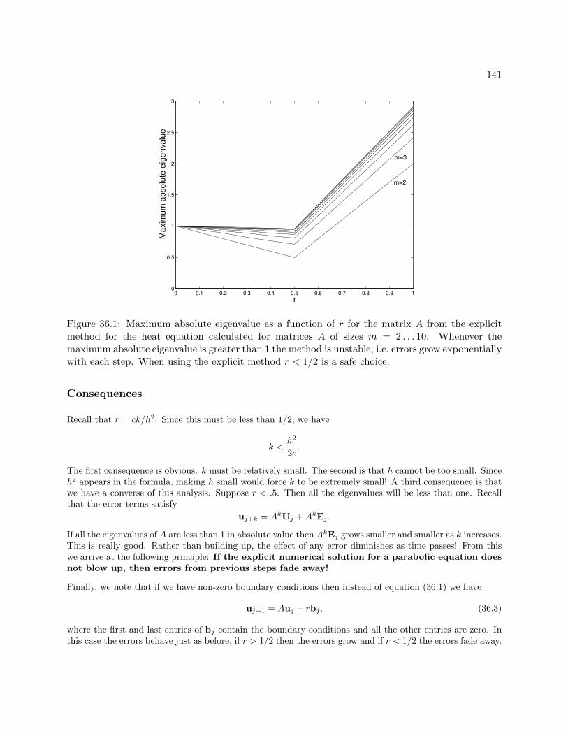
141
0 0.1 0.2 0.3 0.4 0.5 0.6 0.7 0.8 0.9 10
0.5
1
1.5
2
2.5
3
r
Maxim
um
absolu
te e
igenvalu
e
m=2
m=3
Figure 36.1: Maximum absolute eigenvalue as a function of r for the matrix A from the explicitmethod for the heat equation calculated for matrices A of sizes m = 2 . . . 10. Whenever themaximum absolute eigenvalue is greater than 1 the method is unstable, i.e. errors grow exponentiallywith each step. When using the explicit method r < 1/2 is a safe choice.
Consequences
Recall that r = ck/h2. Since this must be less than 1/2, we have
k <h2
2c.
The first consequence is obvious: k must be relatively small. The second is that h cannot be too small. Sinceh2 appears in the formula, making h small would force k to be extremely small! A third consequence is thatwe have a converse of this analysis. Suppose r < .5. Then all the eigenvalues will be less than one. Recallthat the error terms satisfy
uj+k = AkUj +AkEj .
If all the eigenvalues of A are less than 1 in absolute value then AkEj grows smaller and smaller as k increases.This is really good. Rather than building up, the effect of any error diminishes as time passes! From thiswe arrive at the following principle: If the explicit numerical solution for a parabolic equation doesnot blow up, then errors from previous steps fade away!
Finally, we note that if we have non-zero boundary conditions then instead of equation (36.1) we have
uj+1 = Auj + rbj , (36.3)
where the first and last entries of bj contain the boundary conditions and all the other entries are zero. Inthis case the errors behave just as before, if r > 1/2 then the errors grow and if r < 1/2 the errors fade away.
142 LECTURE 36. SOLUTION INSTABILITY FOR THE EXPLICIT METHOD
We can write a function program myexppmatrix that produces the matrix A in (36.2), for given inputs mand r. Without using loops we can use the diag command to set up the matrix:
function A = myexpmatrix(m,r)
% produces the matrix for the explicit method for a parabolic equation
% Inputs: m -- the size of the matrix
% r -- the main parameter , ck/h^2
% Output: A -- an m by m matrix
u = (1-2*r)*ones(m,1); % make a vector for the main diagonal
v = r*ones(m-1 ,1); % make a vector for the upper and lower diagonals
A = diag(u) + diag(v,1) + diag(v,-1); % assemble
end
Test this using m = 6 and r = .4, .6. Check the eigenvalues and eigenvectors of the resulting matirices:
A = myexpmatrix (6 ,.6)
[v e] = eig(A)
What is the “mode” represented by the eigenvector with the largest absolute eigenvalue? How is thatreflected in the unstable solutions?
Exercises
36.1 Let L = π, T = 20, f(x) = .1 sin(x), g1(t) = 0, g2(t) = 0, c = .5, and m = 20, as used in the programmyheat.m. What value of n corresponds to r = 1/2? Try different n in myheat.m to find preciselywhen the method works and when it fails. Is r = 1/2 the boundary between failure and success? Handin a plot of the last success and the first failure. Include the values of n and r in each.
36.2 Write a well-commented Matlab script program that produces the graph in Figure 36.1 for m = 4.Your program should:
• define r values from 0 to 1,
• for each r
– create the matrix A by calling myexppmatrix,
– calculate the eigenvalues of A,
– find the max of the absolute values, and
• plot these numbers versus r.

Lecture 37
Implicit Methods
The Implicit Difference Equations
By approximating uxx and ut at tj+1 rather than tj , and using a backwards difference for ut, the equationut = cuxx is approximated by
ui,j+1 − ui,jk
=c
h2(ui−1,j+1 − 2ui,j+1 + ui+1,j+1).
Note that all the terms have index j + 1 except one and isolating this term leads to
ui,j = −rui−1,j+1 + (1 + 2r)ui,j+1 − rui+1,j+1 for 1 ≤ i ≤ m− 1, (37.1)
where r = ck/h2 as before. The entries involved in (37.1) are illustrated in Figure 37.1.
Now we have uj given in terms of uj+1. This seems like a problem, since uj+1 is the solution at a later timethan uj , so we could never know uj+1 before we knew uj . However, the relationship between uj+1 and ujis linear. Using matrix notation, we have
uj = Buj+1 − rbj+1,
where bj+1 represents the boundary condition. Thus to find uj+1 from uj , we need only solve the linearsystem
Buj+1 = uj + rbj+1 , (37.2)
where uj and bj+1 are given and
B =
1 + 2r −r−r 1 + 2r −r
. . .. . .
. . .
−r 1 + 2r −r−r 1 + 2r
. (37.3)
Using this scheme is called the implicit method since uj+1 is defined implicitly. Since we have to solve alinear system at each step, the implicit is more work per step than the explicit method.
Since we are solving (37.2), the most important quantity is the maximum absolute eigenvalue of B−1, whichis 1 divided by the smallest eigenvalue of B. Figure 37.2 shows the maximum absolute eigenvalues of B−1
as a function of r for various size matrices. Notice that this absolute maximum is always less than 1. Thuserrors are always diminished over time and so this method is always stable. For the same reason it is alsoalways as accurate as the individual steps.
143
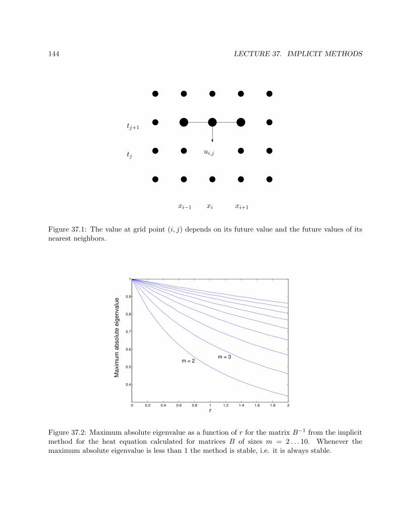
144 LECTURE 37. IMPLICIT METHODS
x x x x xx x ui,j
x xx | | | xx x x x x
?
tj
tj+1
xi−1 xi xi+1
Figure 37.1: The value at grid point (i, j) depends on its future value and the future values of itsnearest neighbors.
0 0.2 0.4 0.6 0.8 1 1.2 1.4 1.6 1.8 2
0.4
0.5
0.6
0.7
0.8
0.9
1
r
Ma
xim
um
ab
so
lute
eig
en
va
lue
m = 2m = 3
Figure 37.2: Maximum absolute eigenvalue as a function of r for the matrix B−1 from the implicitmethod for the heat equation calculated for matrices B of sizes m = 2 . . . 10. Whenever themaximum absolute eigenvalue is less than 1 the method is stable, i.e. it is always stable.

145
Both this implicit method and the explicit method in the previous lecture make O(h2) error in approximatinguxx and O(k) error in approximating ut, so they have total error O(h2 + k). Thus although the stabilitycondition allows the implicit method to use arbitrarily large k, to maintain accuracy we still need k ∼ h2.
Crank-Nicholson Method
Now that we have two different methods for solving parabolic equation, it is natural to ask, “can we improveby taking an average of the two methods?” The answer is yes.
We implement a weighted average of the two methods by considering an average of the approximations ofuxx at j and j + 1. This leads to the equations
ui,j+1 − ui,jk
=λc
h2(ui−1,j+1 − 2ui,j+1 + ui+1,j+1) +
(1− λ)c
h2(ui−1,j − 2ui,j + ui+1,j). (37.4)
The implicit method contained in these equations is called the Crank-Nicholson method. Gatheringterms yields the equations
−rλui−1,j+1 + (1 + 2rλ)ui,j+1 − rλui+1,j+1 = r(1− λ)ui−1,j + (1− 2r(1− λ))ui,j + r(1− λ)ui+1,j .
In matrix notation this isBλuj+1 = Aλuj + rbj+1,
where
Aλ =
1− 2(1− λ)r (1− λ)r
(1− λ)r 1− 2(1− λ)r (1− λ)r. . .
. . .. . .
(1− λ)r 1− 2(1− λ)r (1− λ)r(1− λ)r 1− 2(1− λ)r
and
Bλ =
1 + 2rλ −rλ−rλ 1 + 2rλ −rλ
. . .. . .
. . .
−rλ 1 + 2rλ −rλ−rλ 1 + 2rλ
.
In this equation uj and bj+1 are known, Auj can be calculated directly, and then the equation is solved foruj+1.
If we choose λ = 1/2, then we are in effect doing a central difference for ut, which has error O(k2). Ourtotal error is then O(h2 + k2). With a bit of work, we can show that the method is always stable, and so wecan use k ∼ h without a problem.
To get optimal accuracy with a weighted average, it is always necessary to use the right weights. For theCrank-Nicholson method with a given r, we need to choose
λ =r − 1/6
2r.
This choice will make the method have truncation error of order O(h4 +k2), which is really good consideringthat the implicit and explicit methods each have truncation errors of order O(h2 + k). Surprisingly, we can
146 LECTURE 37. IMPLICIT METHODS
do even better if we also require
r =
√5
10≈ 0.22361,
and, consequently,
λ =3−√
5
6≈ 0.12732.
With these choices, the method has truncation error of order O(h6), which is absolutely amazing.
To appreciate the implications, suppose that we need to solve a problem with 4 significant digits. If we usethe explicit or implicit method alone then we will need h2 ≈ k ≈ 10−4. If L = 1 and T ≈ 1, then we needm ≈ 100 and n ≈ 10, 000. Thus we would have a total of 1, 000, 000 grid points, almost all on the interior.This is a lot.
Next suppose we solve the same problem using the optimal Crank-Nicholson method. We would needh6 ≈ 10−4 which would require us to take m ≈ 4.64, so we would take m = 5 and have h = 1/5. For kwe need k = (
√5/10)h2/c. If c = 1, this gives k =
√5/250 ≈ 0.0089442 so we would need n ≈ 112 to get
T ≈ 1. This gives us a total of 560 interior grid points, or, a factor of 1785 fewer than the explicit or implicitmethod alone.
Exercises
37.1 Modify the program myexppmatrix from exercise 36.2 into a function program myimpmatrix thatproduces the matrix B in (37.3) for given inputs m and r. Modify your script from exercise 36.2 touse B−1 for m = 4 and to plot for r ∈ [0, 2]. It should produce a graph similar to that in Figure 37.2for m = 4. Turn in the programs and the plot.
Lecture 38
Insulated Boundary Conditions
Insulation
In many of the previous sections we have considered fixed boundary conditions, i.e. u(0) = a, u(L) = b. Weimplemented these simply by assigning uj0 = a and ujn = b for all j.
We also considered variable boundary conditions, such as u(0, t) = g1(t). For example, we might haveu(0, t) = sin(t) which could represents periodic heating and cooling of the end at x = 0.
A third important type of boundary condition is called the insulated boundary condition. It is so namedbecause it mimics an insulator at the boundary. Physically, the effect of insulation is that no heat flowsacross the boundary. This means that the temperature gradient is zero, which implies that we should requirethe mathematical boundary condition u′(L) = 0.
To use it in a program, we must replace u′(L) = 0 by a discrete version. Recall that in our discrete equationswe usually have L = xn. Recall from the section on numerical derivatives, that there are three different waysto replace a derivative by a difference equation, left, right and central differences. The three of them at xnwould be
u′(xn) ≈ un − un−1h
≈ un+1 − unh
≈ un+1 − un−12h
.
If xn is the last node of our grid, then it is clear that we cannot use the right or central difference, but arestuck with the first of these. Setting that expression to zero implies
un = un−1.
This restriction can be easily implemented in a program simply by putting a statement u(n+1)=u(n) insidethe loop that updates values of the profile. However, since this method replaces u′(L) = 0 by an expressionthat is only accurate to first order, it is not very accurate and is usually avoided.
Instead we want to use the most accurate version, the central difference. For that we should have
u′(L) = u′(xn) =un+1 − un−1
2h= 0.
or simplyun+1 = un−1.
However, un+1 would represent u(xn+1) and xn+1 would be L + h, which is outside the domain. This,however, is not an obstacle in a program. We can simply extend the grid to one more node, xn+1, and letun+1 always equal un−1 by copying un−1 into un+1 whenever un−1 changes. The point xn+1 is “fictional”,but a computer does not know the difference between fiction and reality! This idea is carried out in thecalculations of the next section and illustrated in Figure 38.1.
147
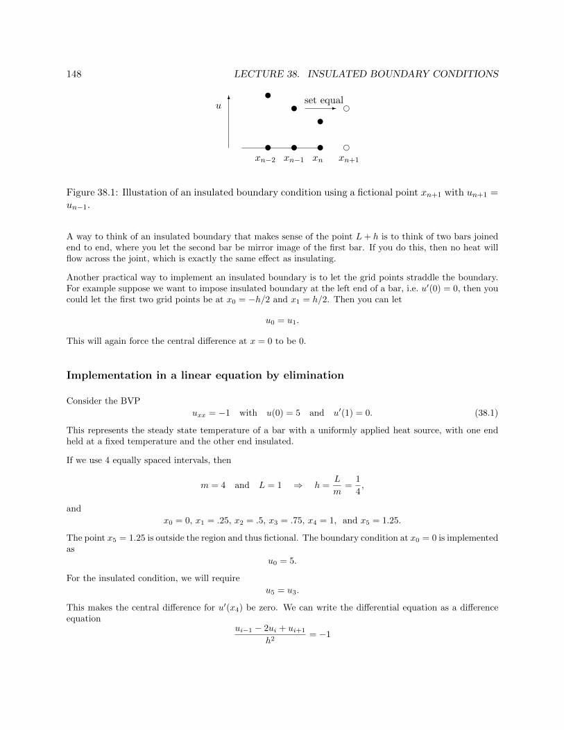
148 LECTURE 38. INSULATED BOUNDARY CONDITIONS
6u
u u u e
u u u e-set equal
xn−2 xn−1 xn xn+1
Figure 38.1: Illustation of an insulated boundary condition using a fictional point xn+1 with un+1 =un−1.
A way to think of an insulated boundary that makes sense of the point L+ h is to think of two bars joinedend to end, where you let the second bar be mirror image of the first bar. If you do this, then no heat willflow across the joint, which is exactly the same effect as insulating.
Another practical way to implement an insulated boundary is to let the grid points straddle the boundary.For example suppose we want to impose insulated boundary at the left end of a bar, i.e. u′(0) = 0, then youcould let the first two grid points be at x0 = −h/2 and x1 = h/2. Then you can let
u0 = u1.
This will again force the central difference at x = 0 to be 0.
Implementation in a linear equation by elimination
Consider the BVP
uxx = −1 with u(0) = 5 and u′(1) = 0. (38.1)
This represents the steady state temperature of a bar with a uniformly applied heat source, with one endheld at a fixed temperature and the other end insulated.
If we use 4 equally spaced intervals, then
m = 4 and L = 1 ⇒ h =L
m=
1
4,
and
x0 = 0, x1 = .25, x2 = .5, x3 = .75, x4 = 1, and x5 = 1.25.
The point x5 = 1.25 is outside the region and thus fictional. The boundary condition at x0 = 0 is implementedas
u0 = 5.
For the insulated condition, we will require
u5 = u3.
This makes the central difference for u′(x4) be zero. We can write the differential equation as a differenceequation
ui−1 − 2ui + ui+1
h2= −1
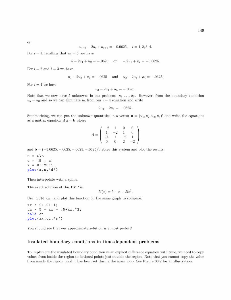
149
orui−1 − 2ui + ui+1 = −0.0625, i = 1, 2, 3, 4.
For i = 1, recalling that u0 = 5, we have
5− 2u1 + u2 = −.0625 or − 2u1 + u2 = −5.0625.
For i = 2 and i = 3 we have
u1 − 2u2 + u3 = −.0625 and u2 − 2u3 + u4 = −.0625.
For i = 4 we haveu3 − 2u4 + u5 = −.0625 .
Note that we now have 5 unknowns in our problem: u1, . . . , u5. However, from the boundary conditionu5 = u3 and so we can eliminate u5 from our i = 4 equation and write
2u3 − 2u4 = −.0625 .
Summarizing, we can put the unknown quantities in a vector u = (u1, u2, u3, u4)′ and write the equationsas a matrix equation Au = b where
A =
−2 1 0 01 −2 1 00 1 −2 10 0 2 −2
and b = (−5.0625,−.0625,−.0625,−.0625)′. Solve this system and plot the results:
u = A\b
u = [5 ; u]
x = 0:.25:1
plot(x,u,’d’)
Then interpolate with a spline.
The exact solution of this BVP is:U(x) = 5 + x− .5x2.
Use hold on and plot this function on the same graph to compare:
xx = 0:.01:1;
uu = 5 + xx - .5*xx.^2;
hold on
plot(xx ,uu ,’r’)
You should see that our approximate solution is almost perfect!
Insulated boundary conditions in time-dependent problems
To implement the insulated boundary condition in an explicit difference equation with time, we need to copyvalues from inside the region to fictional points just outside the region. Note that you cannot copy the valuefrom inside the region until it has been set during the main loop. See Figure 38.2 for an illustration.

150 LECTURE 38. INSULATED BOUNDARY CONDITIONS
y y y yy y y yy y y yy y y y
6 6 6 6
6 6 6 6
6 6 6 6
@@
@@I
@@
@@I
@@@@I
@@
@@I
@@
@@I
@@
@@I
@@@@I
@@
@@I
@@
@@I
@@
@@I
@@@@I
@@
@@I
@@
@@I
AAAAAAAAK
BBBBBBBBBBBBM
CCCCCCCCCCCCCCCCCCO
tj
tj+1
xm−2 xm−1 xm = L g2
y y y y iy y y y iy y y y iy y y y i
6 6 6 6
6 6 6 6
6 6 6 6
@@
@@I
@@
@@I
@@@@I
@@
@@I
@@
@@I
@@
@@I
@@
@@I
@@@@I
@@
@@I
@@
@@I
@@
@@I
@@
@@I
@@@@I
@@
@@I
@@
@@I
R
R
R
R
tj
tj+1
xm−2 xm−1 xm = L
fictional
Figure 38.2: Illustration of information flow for the explicit method near the right boundary atx = L. The top figure shows a fixed boundary condition, where um,j is set to be g2(tj). Thebottom figure shows an insulating boundary condition. Now um,j is updated in the same way asthe general ui,j and an additional entry um+1,j is used with its value set by copying um−1,j .

151
An example
The steady state temperature u(r) (given in polar coordinates) of a disk subjected to a radially symmetricheat load g(r) and cooled by conduction to the rim of the disk and radiation to its environment is determinedby the boundary value problem
∂2u
∂r2+
1
r
∂u
∂r= d(u4 − u4b)− g(r) with u(R) = uR and u′(0) = 0. (38.2)
Here ub is the (fixed) background temperature and uR is the (fixed) temperature at the rim of the disk.
The class web site has a program myheatdisk.m that implements these equations for parameter values R = 5,d = .1, uR = ub = 10 and g(r) = (r − 5)2. Notice that the equations have a singularity (discontinuity) atr = 0. How does the program avoid this problem? How does the program implement uR = 10 and u′(0) = 0?Run the program.
Exercises
38.1 Redo the calculations for the BVP (38.1) except do not include the fictional point x5. Instead, let x4be the last point and impose the insulated boundary by requiring u4 = u3. (Your system of equationsshould be 3 × 3.) Compare this solution with the true solution and the better approximation in thelecture. Illustrate this comparison on a single plot.
38.2 Modify the program myheat.m to have an insulated boundary at x = L (rather than u(L, t) = g2(t)).You will need to change the domain to: x = 0:h:L+h and change the dimensions of all the otherobjects to fit this domain. Run the program with L = 2π, T = 20, c = .5, g1(t) = sin(t) andf(x) = − sin(x/4). Set m = 20 and experiment with n. Get a plot when the program is stable. Turnin your program and plots.

Lecture 39
Finite Difference Method for Elliptic PDEs
Examples of Elliptic PDEs
Elliptic PDE’s are equations with second derivatives in space and no time derivative. The most importantexamples are Laplace’s equation
∆u = uxx + uyy + uzz = 0
and the Poisson equation∆u = f(x, y, z).
These equations are used in a large variety of physical situations such as: steady state heat problems, steadystate chemical distributions, electrostatic potentials, elastic deformation and steady state fluid flows.
For the sake of clarity we will only consider the two dimensional problem. A good model problem in thisdimension is the elastic deflection of a membrane. Suppose that a membrane such as a sheet of rubber isstretched across a rectangular frame. If some of the edges of the frame are bent, or if forces are applied tothe sheet then it will deflect by an amount u(x, y) at each point (x, y). This u will satify the boundary valueproblem:
uxx + uyy = f(x, y) for (x, y) in R,
u(x, y) = g(x, y) for (x, y) on ∂R,(39.1)
where R is the rectangle, ∂R is the edge of the rectangle, f(x, y) is the force density (pressure) applied ateach point and g(x, y) is the deflection at the edge.
The Finite Difference Equations
Suppose the rectangle is described by
R = a ≤ x ≤ b, c ≤ y ≤ d.
We will divide R in subrectangles. If we have m subdivisions in the x direction and n subdivisions in the ydirection, then the step size in the x and y directions respectively are
h =b− am
and k =d− cn
.
We obtain the finite difference equations for (39.1) by replacing uxx and uyy by their central differences toobtain
ui+1,j − 2uij + ui−1,jh2
+ui,j+1 − 2uij + ui,j−1
k2= f(xi, yj) = fij (39.2)
152
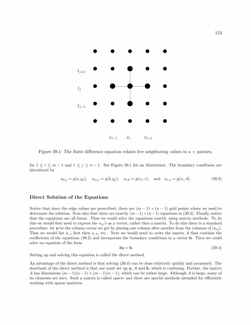
153
x x x x xx x | x xx | | | xx x | x xx x x x x
tj−1
tj
tj+1
xi−1 xi xi+1
Figure 39.1: The finite difference equation relates five neighboring values in a + pattern.
for 1 ≤ i ≤ m − 1 and 1 ≤ j ≤ n − 1. See Figure 39.1 for an illustration. The boundary conditions areintroduced by
u0,j = g(a, yj), um,j = g(b, yj), ui,0 = g(xi, c), and ui,n = g(xi, d). (39.3)
Direct Solution of the Equations
Notice that since the edge values are prescribed, there are (m − 1) × (n − 1) grid points where we need todetermine the solution. Note also that there are exactly (m−1)× (n−1) equations in (39.2). Finally, noticethat the equations are all linear. Thus we could solve the equations exactly using matrix methods. To dothis we would first need to express the uij ’s as a vector, rather then a matrix. To do this there is a standardprocedure: let u be the column vector we get by placing one column after another from the columns of (uij).Thus we would list u:,1 first then u:,2, etc.. Next we would need to write the matrix A that contains thecoefficients of the equations (39.2) and incorporate the boundary conditions in a vector b. Then we couldsolve an equation of the form
Au = b. (39.4)
Setting up and solving this equation is called the direct method.
An advantage of the direct method is that solving (39.4) can be done relatively quickly and accurately. Thedrawback of the direct method is that one must set up u, A and b, which is confusing. Further, the matrixA has dimensions (m− 1)(n− 1)× (m− 1)(n− 1), which can be rather large. Although A is large, many ofits elements are zero. Such a matrix is called sparse and there are special methods intended for efficientlyworking with sparse matrices.

154 LECTURE 39. FINITE DIFFERENCE METHOD FOR ELLIPTIC PDES
Iterative Solution
A usually preferred alternative to the direct method described above is to solve the finite difference equationsiteratively. To do this, first solve (39.2) for uij , which yields
uij =1
2(h2 + k2)
(k2(ui+1,j + ui−1,j) + h2(ui,j+1 + ui,j−1)− h2k2fij
). (39.5)
This method is another example of a relaxation method. Using this formula, along with (39.3), we can updateuij from its neighbors, just as we did in the relaxation method for the nonlinear boundary value problem.If this method converges, then the result is an approximate solution.
The iterative solution is implemented in the script program mypoisson.m on the class web site. Downloadand read it. You will notice that maxit is set to 0. Thus the program will not do any iteration, but will plotthe initial guess. The initial guess in this case consists of the proper boundary values at the edges, and zeroeverywhere in the interior. To see the solution evolve, gradually increase maxit.
Exercises
39.1 Modify the program mypoisson.m (from the class web page) in the following ways:
• Change x = b to be an insulated boundary, i.e. ux(b, y) = 0.
• Change the force f(x, y) to a negative constant −p.
Experiment with various values of p and maxit. Obtain plots for small and large p. Tell how manyiterations are needed for convergence in each. For large p plot also a couple of intermediate steps.

Lecture 40
Convection-Diffusion Equations*
Exercises
40.1
155
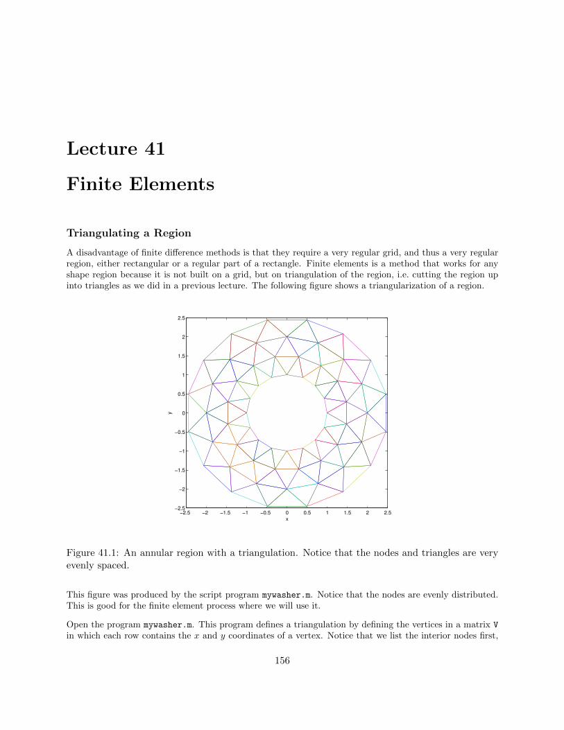
Lecture 41
Finite Elements
Triangulating a Region
A disadvantage of finite difference methods is that they require a very regular grid, and thus a very regularregion, either rectangular or a regular part of a rectangle. Finite elements is a method that works for anyshape region because it is not built on a grid, but on triangulation of the region, i.e. cutting the region upinto triangles as we did in a previous lecture. The following figure shows a triangularization of a region.
−2.5 −2 −1.5 −1 −0.5 0 0.5 1 1.5 2 2.5−2.5
−2
−1.5
−1
−0.5
0
0.5
1
1.5
2
2.5
x
y
Figure 41.1: An annular region with a triangulation. Notice that the nodes and triangles are veryevenly spaced.
This figure was produced by the script program mywasher.m. Notice that the nodes are evenly distributed.This is good for the finite element process where we will use it.
Open the program mywasher.m. This program defines a triangulation by defining the vertices in a matrix V
in which each row contains the x and y coordinates of a vertex. Notice that we list the interior nodes first,
156

157
t
DDDDDDDD
t
BBBBBBBB
t
AAAAAAAA
t
AAAAAAAA
t
BBBBBBBB
tFigure 41.2: The finite elements for the “triangulation” of a one dimensional object.
then the boundary nodes.
Triangles are defined in the matrix T. Each row of T has three integer numbers indicating the indices of thenodes that form a triangle. For instance the first row is 43 42 25, so T1 is the triangle with vertices v43,v42 and v25. The matrix T in this case was produced by the Matlab command delaunay. The commandproduced more triangles than desire and the unwanted ones were deleted.
A three dimensional plot of the region and triangles is produced by having the last line be trimesh(T,x,y,z).
What is a finite element?
The finite element method is a mathematically complicated process. However, a finite element is actuallya very simple object. To each node vj we associate a function Φj that has the properties Φj(vj) = 1 andΦj(vi) = 0 for i 6= j. Between nodes, Φj is a linear function. This function is the finite element. (There arefancier types of finite elements that we will not discuss.)
If we consider one dimension, then a triangulation is just a subdivision into subintervals. In Figure 41.2 weshow an uneven subdivision of an interval and the finite elements corresponding to each node.
In two dimensions, Φj is composed of triangular piece of planes. Thus Φj is a function whose graph is apyramid with its peak over node vj .
What is a finite element solution?
A finite element (approximate) solution is a linear combination of the elements:
U(x) =
n∑j=1
CjΦj(x). (41.1)
Thus finding a finite element solution amounts to finding the best values for the constants Cjnj=1.
In the program mywasher.m, the vector z contains the node values Cj . These values give the height at eachnode in the graph. For instance if we set all equal to 0 except one equal to 1, then the function is a finiteelement. Do this for one boundary node, then for one interior node.
Notice that a sum of linear functions is a linear function. Thus the solution using linear elements is a
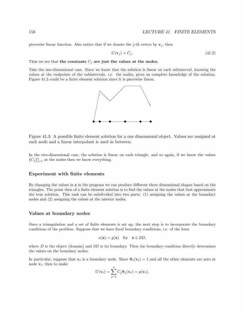
158 LECTURE 41. FINITE ELEMENTS
piecewise linear function. Also notice that if we denote the j-th vertex by vj , then
U(vj) = Cj . (41.2)
Thus we see that the constants Cj are just the values at the nodes.
Take the one-dimensional case. Since we know that the solution is linear on each subinterval, knowing thevalues at the endpoints of the subintervals, i.e. the nodes, gives us complete knowledge of the solution.Figure 41.3 could be a finite element solution since it is piecewise linear.
t
t
@@@
t
t t
AAAAAA
tFigure 41.3: A possible finite element solution for a one dimensional object. Values are assigned ateach node and a linear interpolant is used in between.
In the two-dimensional case, the solution is linear on each triangle, and so again, if we know the valuesCjnj=1 at the nodes then we know everything.
Experiment with finite elements
By changing the values in z in the program we can produce different three dimensional shapes based on thetriangles. The point then of a finite element solution is to find the values at the nodes that best approximatethe true solution. This task can be subdivided into two parts: (1) assigning the values at the boundarynodes and (2) assigning the values at the interior nodes.
Values at boundary nodes
Once a triangulation and a set of finite elements is set up, the next step is to incorporate the boundaryconditions of the problem. Suppose that we have fixed boundary conditions, i.e. of the form
u(x) = g(x) for x ∈ ∂D,
where D is the object (domain) and ∂D is its boundary. Then the boundary condition directly determinesthe values on the boundary nodes.
In particular, suppose that v` is a boundary node. Since Φ`(v`) = 1 and all the other elements are zero atnode v`, then to make
U(v`) =
n∑j=1
CjΦj(v`) = g(v`),

159
we must chooseC` = g(v`).
Thus the constants Cj for the boundary nodes are set at exactly the value of the boundarycondition at the nodes.
Thus, if there are m interior nodes, then
Cj = g(vj), for all m+ 1 ≤ j ≤ n.
In the program mywasher the first 32 vertices correspond to interior nodes and the last 32 correspond toboundary nodes. By setting the last 32 values of z, we achieve the boundary conditions. We could do thisby adding the following commands to the program:
z(33:64) = .5;
or more elaborately we might use functions:
z(33:48) = x(33:48).^2 - .5*y(33:48).^2;
z(49:64) = .2*cos(y(49:64));
Exercises
41.1 Generate an interesting or useful 2-d object and a well-distributed triangulation of it.
• Plot the region.
• Plot one interior finite element.
• Plot one boundary finite element.
• Assign values to the boundary using a function (or functions) and plot the region with theboundary values.
Turn in your code and the four plots.

Lecture 42
Determining Internal Node Values
As seen in the previous section, a finite element solution of a boundary value problem boils down to findingthe best values of the constants Cjnj=1, which are the values of the solution at the nodes. The interiornodes values are determined by variational principles. Variational principles usually amount to minimizinginternal energy. It is a physical principle that systems seek to be in a state of minimal energy and thisprinciple is used to find the internal node values.
Variational Principles
For the differential equations that describe many physical systems, the internal energy of the system is anintegral. For instance, for the steady state heat equation
uxx(x, y) + uyy(x, y) = g(x, y) (42.1)
the internal energy is the integral
I[u] =
∫∫R
u2x(x, y) + u2y(x, y) + 2g(x, y)u(x, y) dA, (42.2)
where R is the region on which we are working. It can be shown that u(x, u) is a solution of (42.1) if andonly if it is minimizer of I[u] in (42.2).
The finite element solution
Recall that a finite element solution is a linear combination of finite element functions:
U(x, y) =
n∑j=1
CjΦj(x, y),
where n is the number of nodes. To obtain the values at the internal nodes, we will plug U(x, y) into theenergy integral and minimize. That is, we find the minimum of
I[U ]
for all choices of Cjmj=1, where m is the number of internal nodes. In this as with any other minimizationproblem, the way to find a possible minimum is to differentiate the quantity with respect to the variables
160

161
and set the results to zero. In this case the free variables are Cjmj=1. Thus to find the minimizer we shouldtry to solve
∂I[U ]
∂Cj= 0 for 1 ≤ j ≤ m. (42.3)
We call this set of equations the internal node equations. At this point we should ask whether the internalnode equations can be solved, and if so, is the solution actually a minimizer (and not a maximizer). Thefollowing two facts answer these questions. These facts make the finite element method practical:
• For most applications the internal node equations are linear.
• For most applications the internal node equations give a minimizer.
We can demonstrate the first fact using an example.
Application to the steady state heat equation
If we plug the candidate finite element solution U(x, y) into the energy integral for the heat equation (42.2),we obtain
I[U ] =
∫∫R
Ux(x, y)2 + Uy(x, y)2 + 2g(x, y)U(x, y) dA. (42.4)
Differentiating with respect to Cj we obtain the internal node equations
0 =
∫∫R
2Ux∂Ux∂Cj
+ 2Uy∂Uy∂Cj
+ 2g(x, y)∂U
∂CjdA for 1 ≤ j ≤ m. (42.5)
Now we have several simplifications. First note that since
U(x, y) =
n∑j=1
CjΦj(x, y),
we have∂U
∂Cj= Φj(x, y) .
Also note that
Ux(x, y) =
n∑j=1
Cj∂
∂xΦj(x, y),
and so∂Ux∂Cj
= (Φj)x.
Similarly,∂Uy
∂Cj= (Φj)y. The integral (42.5) then becomes
0 = 2
∫∫Ux(Φj)x + Uy(Φj)y + g(x, y)Φj(x, y) dA for 1 ≤ j ≤ m.

162 LECTURE 42. DETERMINING INTERNAL NODE VALUES
Next we use the fact that the region R is subdivided into triangles Tipi=1 and the functions in questionhave different definitions on each triangle. The integral then is a sum of the integrals:
0 = 2
p∑i=1
∫∫Ti
Ux(Φj)x + Uy(Φj)y + g(x, y)Φj(x, y) dA for 1 ≤ j ≤ m.
Now note that the function Φj(x, y) is linear on triangle Ti and so
Φij(x, y) = Φj |Ti(x, y) = aij + bijx+ cijy.
This gives us the simplifications
(Φij)x(x, y) = bij and (Φij)y(x, y) = cij .
Also, Ux and Uy restricted to Ti have the form
Ux =
n∑k=1
Ckbik and Uy =
n∑k=1
Ckcik.
The internal node equations then reduce to
0 =
p∑i=1
∫∫Ti
(n∑k=1
Ckbik
)bij +
(n∑k=1
Ckcik
)cij + g(x, y)Φij(x, y) dA for 1 ≤ j ≤ m.
Now notice that (∑nk=1 Ckbik) bij is just a constant on Ti, and, thus, we have
∫∫Ti
(n∑k=1
Ckbik
)bij +
(n∑k=1
Ckcik
)cij =
[(n∑k=1
Ckbik
)bij +
(n∑k=1
Ckcik
)cij
]Ai,
where Ai is just the area of Ti. Finally, we apply the Three Corners rule to make an approximation to theintegral ∫∫
Ti
g(x, y)Φij(x, y) dA .
Since Φij(xk, yk) = 0 if k 6= j and even Φij(xj , yj) = 0 if Ti does not have a corner at (xj , yj), we get theapproximation
Φij(xj , yj)g(xj , yj)Ai/3.
If Ti does have a corner at (xj , yj) then Φij(xj , yj) = 1.
Summarizing, the internal node equations are
0 =
p∑i=1
[(n∑k=1
Ckbik
)bij +
(n∑k=1
Ckcik
)cij +
1
3g(xj , yj)Φij(xj , yj)
]Ai for 1 ≤ j ≤ m.
While not pretty, these equations are in fact linear in the unknowns Cj.
163
Experiment
Download the program myfiniteelem.m from the class web site. This program produces a finite elementsolution for the steady state heat equation without source term:
uxx + uyy = 0 .
To use it, you first need to set up the region and boundary values by running a script such as mywasher ormywedge. Try different settings for the boundary values z. You will see that the program works no matterwhat you choose.
Exercises
42.1 Study for the final!
Review of Part IV
Methods and Formulas
Initial Value Problems
Reduction to First order system:
For an n-th order equation that can be solved for the n-th derivative
x(n) = f
(t, x, x, x, . . . ,
dn−1x
dtn−1
)(42.6)
use the standard change of variables:
y1 = x
y2 = x
...
yn = x(n−1) =dn−1x
dtn−1.
(42.7)
Differentiating results in a first-order system:
y1 = x = y2
y2 = x = y3
...
yn = x(n) = f(t, y1, y2, . . . , yn).
(42.8)
Euler’s method:
yi+1 = yi + hf(ti,yi).
Modified (or Improved) Euler method:
k1 = hf(ti,yi)
k2 = hf(ti + h,yi + k1)
yi+1 = yi +1
2(k1 + k2)
164
165
Boundary Value Probems
Finite Differences:
Replace the Differential Equation by Difference Equations on a grid.Review the lecture on Numerical Differentiation.
Explicit Method Finite Differences for Parabolic PDE (heat):
ut 7→ui,j+1 − uij
kand uxx 7→
ui−1,j − 2uij + ui+1,j
h2(42.9)
leads toui,j+1 = rui−1,j + (1− 2r)ui,j + rui+1,j ,
where h = L/m, k = T/n, and r = ck/h2. The stability condition is r < 1/2.
Implicit Method Finite Differences for Parabolic PDE (heat):
ut 7→ui,j+1 − uij
kand uxx 7→
ui+1,j+1 − 2ui,j+1 + ui−1,j+1
h2(42.10)
leads toui,j = −rui−1,j+1 + (1 + 2r)ui,j+1 − rui+1,j+1,
which is always stable and has truncation error O(h2 + k).
Crank-Nicholson Method Finite Differences for Parabolic PDE (heat):
−rui−1,j+1 + 2(1 + r)ui,j+1 − rui+1,j+1 = rui−1,j + 2(1− r)ui,j + rui+1,j ,
which is always stable and has truncation error O(h2 + k2).
Finite Difference Method for Elliptic PDEs:
uxx + uyy = f(x, y) 7→ ui+1,j − 2uij + ui−1,jh2
+ui,j+1 − 2uij + ui,j−1
k2= f(xi, yj) = fij ,
Finite Elements:
Based on triangles instead of rectangles.Can be used for irregularly shaped objects.An element: Pyramid shaped function at a node.A finite element solution is a linear combination of finite element functions:
U(x, y) =
n∑j=1
CjΦj(x, y),
166 REVIEW OF PART IV
where n is the number of nodes, and where U is an approximation of the true solution.Cj is the value of the solution at node j.Cj at the boundary nodes are given by boundary conditions.Cj at interior nodes are determined by variation principles.The last step in determining Cj ’s is solving a linear system of equations.
Matlab
Initial value problem solver that uses the Runge-Kutta 45 method, which has error O(h5) . The input y0 isthe initial vector and tspan is the time span. You can either make f a vector valued anonymous functionand do
df = @(t,y)[-y(2);y(1)]
[T Y ] = ode45(dy,tspan ,y0)
or make a function program that outputs a vector
function dy = myf(t,y)
dy = [-y(2);y(1)];
end
and then do
[T Y ] = ode45(@myf ,tspan ,y0)
The program ode45 and other Matlab IVP solvers use adaptive step size to achieve a desired local andglobal accuracy, with a default of tol = 10−6 for the global error.
The chief benefit of higher order methods and variable step size is that they allow a program to take onlyas few steps as necessary.

Part V
Appendices
c©Copyright, Todd Young and Martin Mohlenkamp, Department of Mathematics, Ohio University, 2017

Appendix A
Glossary of Matlab Commands
Mathematical Operations
+ Addition. Type help plus for information.
- Subtraction. Type help minus for information.
* Scalar or matrix multiplication. Type help mtimes for information.
/ Scalar or right matrix division. Type help slash for information.
For matrices, the command A/B is equivalent to A*inv(B).
^ Scalar or matrix powers. Type help mpower for information.
.* Element by element multiplication. Type help times for information.
.^ Element by element exponentiation. Type help power for information.
./ Element by element division.
Built-in Mathematical Constants
eps Machine epsilon, i.e. approximately the computer’s floating point roundoff error.
i√−1.
Inf ∞.
NaN Not a number. Indicates an invalid operation such as 0/0.
pi π = 3.14159 . . ..
Built-in Mathematical Functions
abs(x) Absolute value|x|.acos(x) Inverse cosine arccosx.
168
169
asin(x) Inverse sine arcsinx.
atan(x) Inverse tangent arctanx.
cos(x) Cosine cosx.
cosh(x) Hyperbolic cosine coshx.
cot(x) Cotangent cotx.
exp(x) Exponential function ex = expx.
log(x) Natural logarithm lnx = loge x.
sec(x) Secant secx.
sin(x) Sine sinx.
sinh(x) Hyperbolic sine sinhx.
sqrt(x) Square root√x.
tan(x) Tangent tanx.
tanh(x) Hyperbolic tangent tanhx.
max Computes maximum of the rows of a matrix.
mean Computes the average of the rows of a matrix.
min Computes the minimum of the rows of a matrix.
Built-in Numerical Mathematical Operations
fzero Tries to find a zero of the specified function near a starting point or on
a specified interval.
inline Define a function in the command window.
ode113 Numerical multiple step ODE solver.
ode45 Runga-Kutta 45 numerical ODE solver.
quad Numerical integration using an adaptive Simpson’s rule.
dblquad Double integration.
triplequad Triple integration.
Built-in Symbolic Mathematical Operations
collect Collects powers of the specified variable is a given symbolic expression.
compose Composition of symbolic functions.
diff Symbolic differentiation.
double Displays double-precision representation of a symbolic expression.
dsolve Symbolic ODE solver.

170 APPENDIX A. GLOSSARY OF MATLAB COMMANDS
expand Expands an algebraic expression.
factor Factor a polynomial.
int Symbolic integration; either definite or indefinite.
limit Finds two-sided limit, if it exists.
pretty Displays a symbolic expression in a nice format.
simple Simplifies a symbolic expression.
subs Substitutes for parts a a symbolic expression.
sym or syms Create symbolic variables.
symsum Performs a symbolic summation, possibly with infinitely many entries.
taylor Gives a Taylor polynomial approximation of a given order at a specified point.
Graphics Commands
contour Plots level curves of a function of two variables.
contourf Filled contour plot.
ezcontour Easy contour plot.
loglog Creates a log-log plot.
mesh Draws a mesh surface.
meshgrid Creates arrays that can be used as inputs in graphics commands
such as contour, mesh, quiver, and surf.
ezmesh Easy mesh surface plot.
plot Plots data vectors.
ezplot Easy plot for symbolic functions.
plot3 Plots curves in 3-D.
polar Plots in polar coordinates.
quiver Plots a vector field.
semilogy Semilog plot, with logarithmic scale along the vertical direction.
surf Solid surface plot.
trimesh Plot based on a triangulation
trisurf Surface plot based on a triangulation

171
Special Matlab Commands
: Range operator, used for defining vectors and in loops.
Type help colon for information.
; Suppresses output. Also separates rows of a matrix.
= Assigns the variable on the left hand side the value of the right hand side.
ans The value of the most recent unassigned.
cd Change directory.
clear Clears all values and definitions of variables and functions. You may also use to clear only
specified variables.
diary Writes a transcript of a Matlab session to a file.
dir Lists the contents in the current working directory. Same as ls.
help
inline Define an inline function.
format Specifies output format, e.g. > format long.
load Load variables from a file.
save Saves workspace variables to a file.
Matlab Programming
== Is equal?
~= Is not equal?
< Less than?
> Greater than?
<= Less than or equal?
break Breaks out of a for or while loop.
end Terminates an if, for or while statement.
else Alternative in an if statement.
error Displays and error message and ends execution of a program.
for Repeats a block of commands a specified number of times.
function First word in a function program.
if Checks a condition before executing a block of statements.
return Terminates execution of a program.
warning Displays a warning message.
while Repeats a block of commands as long as a condition is true.

172 APPENDIX A. GLOSSARY OF MATLAB COMMANDS
Commands for Matrices and Linear Algebra
Matrix arithmetic:
A = [ 1 3 -2 5 ; -1 -1 5 4 ; 0 1 -9 0] . . . . . . . . . . . . . . . . . . . . . Manually enter a matrix.
u = [ 1 2 3 4]’
A*u
B = [3 2 1; 7 6 5; 4 3 2]
B*A . . . . . . . . . . . . . . . . . . . . . . . . . . . . . . . . . . . . . . . . . . . . . . . . . . . . . . . . . . . . . . . . . . . . . . . . .multiply B times A.
2*A . . . . . . . . . . . . . . . . . . . . . . . . . . . . . . . . . . . . . . . . . . . . . . . . . . . . . . . . . . . . . . . multiply a matrix by a scalar.
A + A . . . . . . . . . . . . . . . . . . . . . . . . . . . . . . . . . . . . . . . . . . . . . . . . . . . . . . . . . . . . . . . . . . . . . . . . . . . . . add matrices.
A + 3 . . . . . . . . . . . . . . . . . . . . . . . . . . . . . . . . . . . . . . . . . . . . . . . . . add a number to every entry of a matrix.
B.*B . . . . . . . . . . . . . . . . . . . . . . . . . . . . . . . . . . . . . . . . . . . . . . . . . . . . . . . . . . . . component-wise multiplication.
B.^3 . . . . . . . . . . . . . . . . . . . . . . . . . . . . . . . . . . . . . . . . . . . . . . . . . . . . . . . . . . . .component-wise exponentiation.
Special matrices:
I = eye(3) . . . . . . . . . . . . . . . . . . . . . . . . . . . . . . . . . . . . . . . . . . . . . . . . . . . . . . . . . . . . . . . . . . . . . identity matrix
D = ones(5,5)
O = zeros(10,10)
C = rand(5,5) . . . . . . . . . . . . . . . . . . . . . . . . . . . . . . . random matrix with uniform distribution in [0, 1].
C = randn(5,5) . . . . . . . . . . . . . . . . . . . . . . . . . . . . . . . . . . . . . . . random matrix with normal distribution.
hilb(6)
pascal(5)
General matrix commands:
size(C) . . . . . . . . . . . . . . . . . . . . . . . . . . . . . . . . . . . . . . . . . . . . . . . . . . . . . gives the dimensions (m× n) of A.
norm(C) . . . . . . . . . . . . . . . . . . . . . . . . . . . . . . . . . . . . . . . . . . . . . . . . . . . . . . . . . . . gives the norm of the matrix.
det(C) . . . . . . . . . . . . . . . . . . . . . . . . . . . . . . . . . . . . . . . . . . . . . . . . . . . . . . . . . . .the determinant of the matrix.
max(C) . . . . . . . . . . . . . . . . . . . . . . . . . . . . . . . . . . . . . . . . . . . . . . . . . . . . . . . . . . . . . . . the maximum of each row.
min(C) . . . . . . . . . . . . . . . . . . . . . . . . . . . . . . . . . . . . . . . . . . . . . . . . . . . . . . . . . . . . . . . the minimum in each row.
sum(C) . . . . . . . . . . . . . . . . . . . . . . . . . . . . . . . . . . . . . . . . . . . . . . . . . . . . . . . . . . . . . . . . . . . . . . . . . . sums each row.
mean(C) . . . . . . . . . . . . . . . . . . . . . . . . . . . . . . . . . . . . . . . . . . . . . . . . . . . . . . . . . . . . . . . . the average of each row.
diag(C) . . . . . . . . . . . . . . . . . . . . . . . . . . . . . . . . . . . . . . . . . . . . . . . . . . . . . . . . . . . . . just the diagonal elements.
inv(C) . . . . . . . . . . . . . . . . . . . . . . . . . . . . . . . . . . . . . . . . . . . . . . . . . . . . . . . . . . . . . . . . . . . . inverse of the matrix.

173
Matrix decompositions:
[L U P] = lu(C)
[Q R] = qr(C)
[U S V] = svd(C) . . . . . . . . . . . . . . . . . . . . . . . . . . . . . . . . . . . . . . . . . . . . . . . . singular value decomposition.

174 APPENDIX A. GLOSSARY OF MATLAB COMMANDS