introduction - university of california, irvinein terms of savage’s discussion of small worlds and...

INDUCTIVE LEARNING IN SMALL AND LARGE WORLDS

SIMON M. HUTTEGGER

1. Introduction

Bayesian treatments of inductive inference and decision making presuppose thatthe structure of the situation under consideration is fully known. We are, however,often faced with having only very fragmentary information about an epistemicsituation. This tension was discussed in decision theory by Savage (1954) in termsof ‘small worlds’ and ‘large worlds’ (‘grand worlds’ in Savage’s terminology). Largeworlds allow a more fine grained description of a situation than small worlds. Theadditional distinctions may not be readily accessible, though. Savage realized thatplanning ahead is difficult, if not impossible, whenever we don’t have sufficientknowledge of the the basic structure of an epistemic situation. Since planning isat the heart of Bayesian inductive inference and decision making, it is not easyto see how a Bayesian—or any learner, for that matter—can deal with incompleteinformation.

The aim of this paper is to outline how the mathematical and philosophical foun-dations of inductive learning in large worlds may be developed. First I wish to showthat there is an important sense in which Bayesian solutions for inductive learningin large worlds exist. The basic idea is the following: Even if one’s knowledge ofa situation is incomplete and restricted, Bayesian methods can be applied basedon the information that is available. This idea is more fully developed in §§4, 5and 6 for two concrete inductive learning rules that I introduce in §2. Importantly,however, this does not always lead to fully rational inductive learning: the analysisof a learning rule within the confines of the available information is by itself notsufficient to establish its rationality in larger contexts. In §3 I couch this problemin terms of Savage’s discussion of small worlds and large worlds. I take this threadup again in §7, where inductive learning in small and large worlds is examinedin the light of bounded rationality and Richard Jeffrey’s epistemology of ‘radicalprobabilism’.

2. Two Learning Rules

In order to fix ideas we introduce two abstract models of learning. Both modelsprovide rules for learning in a decision context. The decision context is convenientfor developing a theory of learning in large and small worlds, but it is by no meansnecessary, as I hope to make clear at the end of this section.

Suppose that nature has K states {1, . . . ,K} which are chosen repeatedly, result-ing in a sequence of states. We don’t make any assumptions about the process that

Date: July 2015.I would like to thank Brian Skyrms, Elliott Wagner and Kevin Zollman for comments on earlierdrafts of this paper. This paper was presented at the University of Groningen, where the audienceprovided helpful .

1

2 SIMON M. HUTTEGGER

generates this sequence. For example, in a stationary environment nature mightchoose each state i with a fixed probability pi, the choices being independent. Al-ternatively, the sequence of states of nature could be a stationary Markov chain.But mother nature need not be stationary: the states might also be the strategicchoices of players in a game theoretic environment.

We assume also that there is an agent who can choose among M acts {1, . . . ,M}.The outcome of a choice by nature and a choice by the agent is a state-act pair.For each such pair there is assumed to be a von Neumann-Morgenstern utilitywhich represents the agent’s preferences over outcomes.1 Suppose that the agentcan observe states of nature. She may then have predictive probabilities about thestate that will be observed on the next trial. Let Xn denote the state of nature atthe nth trial. In the language of probability theory, Xn is a random variable thattakes on values in {1, . . . ,K}. For a sequence of states X1, . . . , Xn, let ni be thenumber of times state i has been observed. Then the following is a natural way tocalculate the predictive probability of observing state i on trial n+ 1:

(1) P[Xn+1 = i|X1, . . . , Xn] =ni + αi

n+∑j αj

for i = 1, . . . ,K and some non-negative constants αj . This rule is a generalization ofLaplace’s rule of succession. If all αi are equal to zero, (1) is Reichenbach’s straightrule (Reichenbach, 1949). Provided that some αj are positive, then prior to makingobservations (n = 0) the predictive probability for state i is equal to αi/

∑j αj . By

calculating the expected utility of each act relative to the predictive probabilities(1), the agent can choose an act that maximizes this expected utility. Such anact is called a (myopic) best response. The resulting rule is called fictitious play.Fictitious play was originally conceived as a device for calculating Nash equilibriain games. Since then it has become one of the most important rules studied in thetheory of learning in games, and many of its properties are well understood.2

Fictitious play is a simple form of the dominant Bayesian paradigm; it combinesBayesian conditioning with maximizing expected payoffs. As such, it assumes thatthe agent has the conceptual resources for capturing what states of nature thereare. Note, however, that fictitious play is a fairly simple type of Bayesian learning—Bayesian learners can be vastly more sophisticated. A Bayesian might not justchoose a myopic best response, but might also contemplate the effects of her choiceon future payoffs. Moreover, a Bayesian agent is not required to have predictiveprobabilities that are given by a rule of succession; in general, posterior probabilitiesmight have a much more complex structure.

Some modes of learning need less fine-grained information. The rule we con-sider here does not need information about states but only about acts and payoffs.Suppose that there are L possible payoffs π1 < π2 < · · · < πL (which can againbe thought of as von Neumann-Morgenstern utilities of consequences, ordered fromthe least to the most preferred). Now suppose that the agent has chosen her ithaction ni times, nij of which resulted in payoff πj . Then our second learning rule

1Von Neumann-Morgenstern utilities are given by a cardinal utility function. The utility scale

determined by such a function is unique up to a choice of a zero point and the choice of a unit.See von Neumann and Morgenstern (1944).2Fictitious play was introduced by Brown (1951). For more information see Fudenberg and Levine(1998) and Young (2004). Strictly speaking, one also needs to specify a rule for breaking payoff

ties. In the present context it doesn’t matter which one is adopted.

INDUCTIVE LEARNING IN SMALL AND LARGE WORLDS 3

recommends to choose an act i that maximizes

(2)

∑j πjnij +

∑j πjαij

ni +∑j αij

.

Up to the parameters αij , this is the average payoff that was obtained by act i.If the αij are positive, then

∑j πjαij/

∑j αij can be viewed as the agent’s initial

estimate of act i’s future payoff.The rule (2) is a type of reinforcement learning scheme, where

∑j πjαij is the

agent’s initial propensity for choosing act i and∑j πjnij is the cumulative payoff

associated with act i. After having chosen an act i, the payoff is added to thecumulative payoff for i. The total reinforcement for an act is the sum of the initialpropensity and the cumulative payoff for that act. The act with maximum averagepayoff is then chosen in the next trial. For this reason we call this rule averagereinforcement learning.3 Averaging mitigates the effect of choosing an act veryoften. Such an act may accrue a large cumulative reinforcement even if the payoffsat each trial are very small, and so may look attractive despite not promising asignificant payoff on the next trial.

Fictitious play can also be regarded as a reinforcement learning scheme; but itis of a quite different kind, known as ‘hypothetical reinforcement learning’. In hy-pothetical reinforcement learning cumulative payoffs are not just gotten by addingactually obtained payoffs; the agent also adds the ‘counterfactual’ payoffs she wouldhave gotten if she had chosen other acts (Camerer and Ho, 1999). Fictitious play canuse counterfactual payoff information because knowing the state of nature allowsher to infer what the alternative payoffs would have been. Average reinforcementlearning does not have the conceptual resources to make these inferences.

The difference between average reinforcement learning and fictitious play can alsobe expressed in another way by looking again at their inputs. One fundamentalclassification of learning rules for decision situations is whether or not they arepayoff based.4 Fictitious play is not payoff based because it does not just keep trackof the agent’s own payoffs. Average reinforcement learning, on the other hand, ispayoff based since its only input is information about payoffs.

Both fictitious play and average reinforcement learning choose an act that seemsbest from their point of view. And both rules are inductive in the sense that theytake into account information about the history before choosing an act. Thereare other inductive rules, to be sure. In repeated decision problems of the kinddescribed above, any inductive learning rule has

(i) a ‘conceptual system’ capturing the information that must be available inorder to use that rule and

(ii) a specification of how the rule maps information about the past to futurechoices.

The conceptual system of fictitious play consists of a set of states, a set of acts and aset of outcomes. The conceptual system of average reinforcement learning consistsof a set of acts and a set of outcomes. Fictitious play maps finite sequences of statesto acts (up to a rule that applies when two acts have the same expected utility).Average reinforcement learning maps sequences of pairs of acts and outcomes to

3Rules such as (2) are well known in the literature on bandit problems as ‘greedy’ learning rules,

because they always choose what currently seems best (Berry and Fristedt, 1985).4See Fudenberg and Levine (1998) and Young (2004).


acts (again up to a rule that breaks ties). Alternatively, both rules may be thoughtof as mapping histories to vectors whose components represent the values of acts(expected values and average reinforcements, respectively), or as ordering acts.Other learning rules use different kinds of inputs and map them to choices, eitherdeterministically or probabilistically.

Inductive learning is of course not restricted to repeated decision problems. Ingeneral, we may take an inductive learning rule as a map from finite sequences ofinputs to some types of outputs so that the rule is always defined for increasingsequences of inputs. More formally, let us say that the conceptual system of alearning rule is an ordered set C of sets S1, . . . , Sk, where the elements of each Siare objects that are in some way epistemically accessible to an agent using that rule.The inputs are given by S1, . . . , Sm and the outputs are given by Sm+1, . . . , Sk. Afinite history of inputs is a sequence of elements in S1 × · · · × Sm. An inductivelearning rule maps each finite history to an output (an element in, or a subset ofSm+1 × · · · × Sk). Roughly speaking, sequences of inputs describe what the agenthas learned, while outputs specify what is adjusted in response to learning.5

In the following section we refer to fictitious play, average reinforcement learning,and a decision context. But keep in mind that the approach developed here appliesto inductive learning more generally.

3. Small and Large Worlds

Our two learning rules are interesting not just because of their relevance tolearning in repeated decision situations, but also because the conceptual system ofaverage reinforcement learning is a ‘coarsening’ of the conceptual system of fictitiousplay. This can be seen as follows. We may think of states, acts, and outcomes aspropositions, as Richard Jeffrey does in his logic of decision (Jeffrey, 1965). Thenthe sets of states, acts, and outcomes together define a partition. This partitioncaptures the knowledge structure underlying fictitious play. The conceptual systemof average reinforcement learning, on the other hand, only has the set of actsand the set of outcomes as elements. The partition determined by these two setsis a coarsening of the partition underlying fictitious play. Thus the knowledgestructure of fictitious play is more refined than the knowledge structure of averagereinforcement learning.

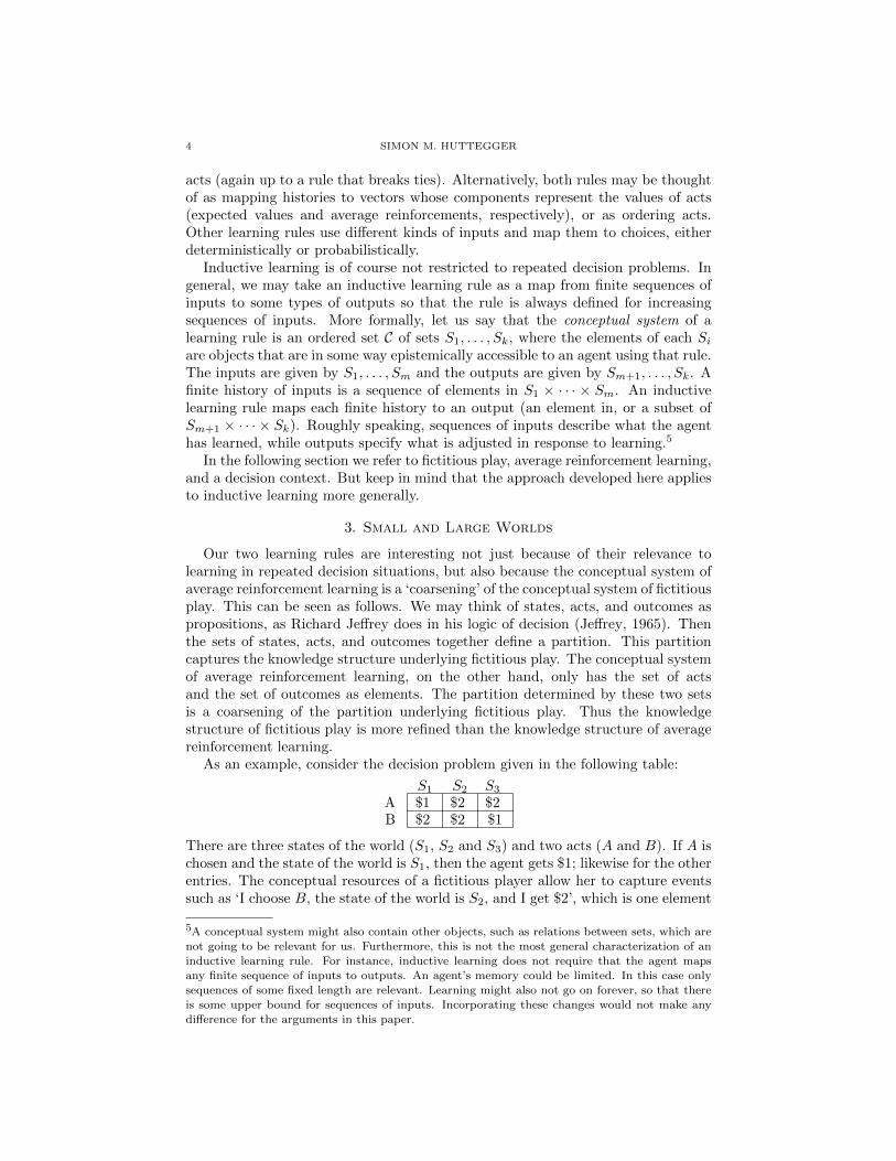
As an example, consider the decision problem given in the following table:

S1 S2 S3

A $1 $2 $2B $2 $2 $1

There are three states of the world (S1, S2 and S3) and two acts (A and B). If A ischosen and the state of the world is S1, then the agent gets $1; likewise for the otherentries. The conceptual resources of a fictitious player allow her to capture eventssuch as ‘I choose B, the state of the world is S2, and I get $2’, which is one element

5A conceptual system might also contain other objects, such as relations between sets, which are

not going to be relevant for us. Furthermore, this is not the most general characterization of aninductive learning rule. For instance, inductive learning does not require that the agent maps

any finite sequence of inputs to outputs. An agent’s memory could be limited. In this case only

sequences of some fixed length are relevant. Learning might also not go on forever, so that thereis some upper bound for sequences of inputs. Incorporating these changes would not make any

difference for the arguments in this paper.


in the partition given by states, acts and outcomes. If she is told that the true stateis neither S1 nor S3, she knows that she cannot win $1. If she is told that she wins$1, then she knows that she cannot be in state S2. The information available toaverage reinforcement learning is less fine grained. Here we can only express eventssuch as ‘I choose B and I get $2’. Each such event is a proper superset of a fictitiousplay event. If in the new partition you are told that you don’t get $1, you onlyknow that you get $2 without knowing which state of the world is the true one.Thus, in a very precise sense, average reinforcement learning does in general notrequire as much information about a decision situation as fictitious play. This istrue for all payoff based learning rules in any decision problem where states are notuniquely identifiable in terms of acts and payoffs, which will be the case wheneverthe payoff of an act is the same in more than one state.

Using a term introduced by Savage (1954), the conceptual system of a payoffbased learning rule may be thought of as a small world. Savage distinguishes smallworlds from large worlds. The large world that pertains to a decision situationis a fully considered description of the decision problem at hand. This meansthat every potentially relevant act, state of the world or outcome has entered thedescription of the decision problem.6 If we again view a decision problem in termsof its associated partition, the large world is the finest partition that is relevantfor a given decision situation. Any small world, on the other hand, is a coarseningof that finest partition that ignores some large world distinctions. In between thelarge world and a particular small world we may have worlds that are smaller orlarger relative to one another. In particular, the world underlying a payoff basedlearning rule such as average reinforcement learning is a smaller world than theworld of fictitious play or other non-payoff based learning methods.

The distinction between small and large worlds is related to another impor-tant topic in decision theory: bounded rationality.7 Bounded rationality goes backmainly to the work of Herbert Simon, who maintained that real world reasoningand decision making is not captured adequately by the standards of high rationalitymodels (e.g. Simon, 1955, 1957). To illustrate this point, consider the extreme caseof a large world, namely, a person’s whole life (Savage, 1954, p. 83). In this largeworld one is choosing how to live, once and for all. This choice is made after havingconsidered the decision situation in full detail. This is evidently unrealistic evenfor agents with fairly sophisticated reasoning powers. For most kinds of agents itis possible to find less extreme large worlds that are beyond the bounds given byplausible epistemic constraints for that type of agent.

What we should take from this discussion is that decision making and inductivelearning nearly always takes place in a small world, that is, a coarsening of anunderlying large world. This allows us to discuss the rationality of learning rulessuch as fictitious play or average reinforcement learning at the small world level orthe large world level. At the small work level we may ask whether a learning ruleis rational within its conceptual system. The kind of rationality I am referring tohere aims at identifying the principles underlying a learning rule. Consider fictitious

6In other words, for a large world decision problem we require that there is no proposition that,when added to the description of the decision situation, would disrupt the agent’s preferences.See Joyce (1999, p. 73) for a more precise definition.7This relationship was recently discussed by, e.g., Binmore (2009), Gigerenzer and Gaissmaier(2011) or Brighton and Gigerenzer (2012).


play, and take its take its conceptual systems as given. We may wonder whetherthe way it calculates predictive probability is just arbitrary or can be based onreasonable principles. The same can be asked with regard to average reinforcementlearning.

This part of the project is to some extent a purely mathematical venture. Itsmethodology is the axiomatic method, which was used very successfully in manyfields of modern mathematics, starting with Hilbert’s foundations of geometry andused by Kolmogorov in his theory of probability. The probabilistic theories ofinductive inference due to Bruno de Finetti and Rudolf Carnap are especially salientfor our project. Both de Finetti and Carnap derive inductive learning rules from aset of basic postulates. In the next section (§4) I explain how these postulates can beused to apply the axiomatic method to fictitious play. At this level, the resultingtheory of inductive learning could be treated as a mathematical theory withoutinterpretation. This would not be satisfying from a philosophical perspective, andboth Carnap and de Finetti thought of their projects as normative epistemologicaltheories. I’ll explain their positions briefly in §5, arguing for a position very closeto de Finetti’s view. On this view, the postulates from which a learning rule canbe derived are inductive assumptions about the basic structure of the learningsituation. If an agent’s beliefs conform to those inductive assumptions, then—sincefictitious play follows deductively from the postulates—it is the only admissiblelearning rule. The agent should adopt fictitious play on pain of inconsistency.

What is new about my approach is that the same methodology can be appliedto average reinforcement learning. Given the differences between average reinforce-ment learning and fictitious play, it might not be immediately obvious that this ispossible. In §6 I show two things: (i) Based on the conceptual system of averagereinforcement learning there is a set of plausible postulates from which that learn-ing rule can be derived, and (ii) these postulates can be thought of as inductiveassumptions. Given that an agent believes a particular set of inductive assump-tions, she has to be an average reinforcement learner on pain of inconsistency. Thisyields the same kind of theory of rational learning as for fictitious play, but for alearning rule with bounded resources.

The normative status of different modes of inductive learning (fictitious play,average reinforcement learning) is based on the consistency between inductive as-sumptions and the learning procedure. Rationality here is correct reasoning withinan abstract small world model of a learning situation. But, as in the case of decisiontheory, the question of whether learning procedures are rational goes beyond thesmall world context. Are the inferences that are judged to be rational in the smallworld also rational in larger worlds? And how is this related to the conceptualabilities of agents? These questions are especially relevant for payoff based learningrules because of their coarse conceptual basis.

The relationship between small and large worlds is an important but also verycomplex question8, and I don’t claim to have a fully satisfying answer to all theseissues. For now let me set aside this discussion. I’ll pick it up again after havinglaid out the small world foundations of learning rules which was outlined in thissection. This will put us in a better position to gain some qualitative insights intothe more complex issues.

8Cf. the discussion in Savage (1954, p. 82-91) and Joyce (1999, p. 70-77).


4. De Finetti’s Theorem and Inductive Logic

The well-known key for providing a foundation for fictitious play is the notionof exchangeability. Exchangeability originated with W. E. Johnson’s permutationpostulate (Johnson, 1924). But not before Bruno de Finetti’s work on exchangeablesequences of random events was it used with full force.

Suppose that X1, X2, . . . is an infinite sequence of random variables (whichmay as in §2 be thought of as recording the occurrences of the states of nature{1, . . . ,K}). The sequence X1, X2, . . . is said to be exchangeable if the probabilityP of any finite initial sequence of states only depends on the number of times eachstate occurs and not on their order. More precisely, let (j1, . . . , jn) be a vector whosecomponents ji are elements of {1, . . . ,K}. Then the sequence is exchangeable if

P[X1 = j1, X2 = j2, . . . , Xn = jn] = P[X1 = jσ(1), X2 = jσ(2), . . . , Xn = jσ(n)]

for any permutation σ of {1, . . . , n} and any n = 1, 2, . . .. If, for example, K = 3,then

P[1, 2, 3] = P[3, 1, 2] = P[2, 3, 1] = P[1, 3, 2] = P[3, 2, 1] = P[2, 1, 3]

because all these sequences have one state 1, one state 2, and one state 3. But itneed not be the case that, e.g., P[1, 1, 2] = P[1, 2, 3].

If the sequence X1, X2, . . . is exchangeable, then de Finetti’s celebrated represen-tation theorem states that the probability measure P is a mixture of independentmultinomial probabilities.9 For i = 1, . . . ,K, let ni be the number of times i isfound among (j1, . . . , jn). Also, let ∆K be the set of all probability distributions(p1, . . . , pK) on the set {1, . . . ,K}, where pi is the probability of i. If X1, X2, . . .is exchangeable, then there exists a unique prior measure dµ on ∆K such that forevery n and every (j1, . . . , jn)

(3) P[X1 = j1, X2 = j2, . . . , Xn = jn] =

∫∆K

pn11 · · · p

nK

K dµ(p)

with n1 + · · ·nK = n and p = (p1, . . . , pK) ∈ ∆K . This theorem has severalremarkable consequences.10 One concerns the metaphysics of chance. A radicalsubjectivist such as de Finetti thinks of objective chances as illusions. Because ofthe representation theorem, a subjectivist is nonetheless licensed to use chances ifher subjective probabilities are exchangeable. The elements in ∆K can be viewedas chance parameters. Given the chance parameters, the agent believes that obser-vations are like trials which are independently and identically distributed accordingto those chance parameters. The mixing measure dµ can be viewed as the agent’sprior beliefs over chances. Yet again, a strict subjectivist would insist that themeasure dµ is nothing but a useful fiction that one is allowed to entertain becauseof the representation theorem.11 An agent does not need to believe in true chances.But if her degrees of beliefs are exchangeable, the agent behaves as if she did.

Another consequence of de Finetti’s theorem is relevant for inductive reasoning.The formula (3) can be used to calculate the conditional probability of observing acertain state given past observations. The past observations determine a posterior

9See de Finetti (1937). There are much more general versions of the theorem. For an excellentsurvey see Aldous (1985).10See Zabell (1989).11This is the main difference between classical Bayesians, such as Laplace and Bayes himself, andmodern subjective Bayesians.


from the prior dµ. The conditional probability of a state given past observations isthen just the chance expectation relative to the posterior.

One concrete instance of this conditional probability turns out to be especiallysalient for our purposes. Suppose the prior measure dµ has a Dirichlet distributionon ∆K .12 A straightforward calculation shows that the conditional probability ofobserving state i at time n+ 1 given all past observations is equal to

ni + αin+

∑j αj

.

Thus, the predictive probabilities in (1) result from the representation theoremwhenever one’s degrees of belief are exchangeable and one has a Dirchlet prior overchances.

De Finetti himself emphasizes the qualitative implications of his theorem for theproblem of induction, and the artificiality of particular choices of prior distributionsover chances.13 This is in line with the view that chance priors are only usefulfictions. Now, Dirichlet priors are certainly mathematically convenient—but isthere a deeper reason for using them as one’s mixing measure?

Inductive logic provides an answer to this question. The type of inductive logicI’m referring to goes back to W. E. Johnson, and was later independently developedby Rudolf Carnap. Inductive logic also starts with exchangeability. But insteadof using Dirichlet priors, Johnson and Carnap assume what is often referred toas ‘Johnson’s sufficientness postulate.’ The sufficientness postulate states that theprobability of observing category i on the next trial only depends on i, the numberni of i’s observed to date, and the total number of trials n:

(4) P[Xn+1 = i|X1, . . . , Xn] = fi(ni, n)

In order for the conditional probabilities in (4) to be well defined, we must have

(5) P[X1 = j1, . . . , Xn = jn] > 0 for all j1, . . . , jn ∈ {1, . . . ,K}.The regularity condition (5) says that each finite initial sequence of observationshas positive prior probability.

It can be proved that if K ≥ 3 the predictive probabilities given in (1) followfrom exchangeability together with (4) and (5).14 Johnson’s sufficientness postulatecan thus be viewed as a characterization of Dirichlet priors. If an agent thinks thatknowledge of i, ni and n is sufficient for determining the probability of i on the

12That is, dµ is

Γ(∑K

j=1 αj

)∏Kj=1 Γ (αj)

pα1−11 · · · pαK−1

K dp1 · · · dpK−1,

where Γ is the gamma function.13E.g. de Finetti (1938). On p. 203 of the translation (where Φ denotes the prior) he writes:“It must be pointed out that precise applications, in which Φ would have a determinate analyticexpression, do not appear to be of much interest: as in the case of exchangeability, the principal

interest of the present methods resides in the fact that the conclusions depend on a gross, qual-itative knowledge of Φ, the only sort we can reasonably suppose to be given (except in artificial

examples).”14For details, see Zabell (1982), who reconstructs the proof sketch from Johnson’s posthumouslypublished article (Johnson, 1932). It has to be assumed that there are at least three states, for

otherwise the sufficientness postulate is empty. If there are only two states, one can either assumethat the predictive probabilities are linear in ni, or consider relevance quotients as in Costantini(1979).


next trial given the outcomes so far, then she acts as if she has a Dirchlet priorover the unknown chances of the K types of observations.

5. Rational Foundations

We see that there are two main approaches to deriving the probabilities usedby fictitious play. One rests on subjective Bayesian probability theory. The otherone is based on inductive logic.15 Both attempts succeed in providing an axiomaticbasis for fictitious play (together with von Neumann-Morgenstern utility theory).However, going beyond the purely mathematical aspect of the theories, we may askin what sense we get a rational foundation from the axiomatic approach.

One view is that assumptions like exchangeability, the sufficientness postulate, orregularity are requirements of rationality—something rational beliefs have to con-form to. Let’s consider exchangeability as an example. At least in his early workon inductive logic, Carnap seems to have thought of exchangeability as a logicalprinciple. Carnap was working within the context of probability functions on sen-tences of a first-order language. In this context exchangeability is the invariance ofprobability under permutations of the individual constants of the language. Basedon the idea of Alfred Lindenbaum and Alfred Tarski that logical properties have tobe invariant under certain transformations of the elements of the language, Carnapviewed exchangeability as a basic a priori principle of inductive logic. Accordingly,one is rationally required to have exchangeable probabilities (Carnap, 1950, §§90,91).

The problem with this idea is that in applications to problems of inductiveinference exchangeability has usually a temporal component, or otherwise refersto known and unknown observations. The information conditioned on involvesobservations that have already been made, and what is predicted is unknown as ofyet. Within the context of inductive logic on a first-order language this means thatthe individual constants are temporally ordered. This results in what Carnap callsa ‘coordinate language.’ But in such a language the principle of exchangeabilityloses its innocence and makes a substantial claim about what the agent expects toobserve.16 The claim is that the observations one expects to make are homogenous.It is not easy to see how one can uphold the logicality of exchangeability or othersymmetry principles in the face of the very concrete claims they make about randomprocesses.17

De Finetti and other subjective Bayesians offer a different vision of the ratio-nality of learning rules. On this view, exchangeability or Johnson’s sufficientnesspostulate are not taken as having the status of necessary principles. Instead, theyare an agent’s personal judgements, or inductive assumptions, regarding the basicstructure of her observations.18 Inductive assumptions are basic facts about anagent’s prior probability. They express the agent’s beliefs about the whole learningsituation rather than just some aspects of it. Exchangeability is a prime example ofan inductive assumption. It says that all trials are completely analogous; it doesn’tmake a difference whether you observe an outcome on the first trial or on a later

15The two are closely related; see Skyrms (1996).16Carnap was well aware of this point; see Carnap (1971, 118-120)17For a thorough discussion of these issues see Zabell (1989).18I borrow the term ‘inductive assumptions’ from Howson (2000).


trial. Exchangeability is thus a symmetry or invariance principle. Inductive as-sumptions are often expressed as symmetry principles. Such principles tell us whatan agent thinks is of relevance about the whole learning situation.

What distinguishes de Finetti’s subjectivistic view from the logical view of Car-nap is that an agent is not required to have exchangeable degrees of belief butis allowed to use other symmetries (like the one discussed in the next section).But then, what makes inductive learning rational on the subjectivistic view if in-ductive assumptions (exchangeability, sufficientness postulate) are not themselvesrequirements of rationality? The rationality of an inductive learning rule is dueto its being consistent with the agent’s inductive assumptions. For instance, theCarnapian predictive probabilities (1) follow from exchangeability, Johnson’s suffi-cientness postulate, and regularity. If the agent accepts these assumptions, she isbound to learn from experience according to a generalized rule of succession. Infact, it is easy to see that all three conditions are necessary for Carnapian predictiveprobabilities. It would be inconsistent to claim that one’s conditional probabilitiesare Carnpian predictive probabilities while to deny at the same time that, say, one’sunconditional probabilities are exchangeable.

The modest subjectivist understanding of rational learning is thus not as sweep-ing as some might wish. This is not the place to explain why it is the correctposition; de Finetti and others have forcefully argued for it in many places.19 I’monly going to make a few remarks concerning the epistemic status of inductive as-sumptions. If they are not rationality postulates, how are they justified? Let’sagain consider exchangeability. It is a property of an agent’s degrees of belief. Howdoes an agent come to hold exchangeable degrees of belief? In some cases, she mighthave good reasons for it. For example, our agent ’s judgment that a sequence of coinflips is exchangeable might be based on past experiences with similar coins. Butde Finetti and other subjective Bayesians do not insist upon inductive assumptionshaving this kind of epistemic warrant. The reason is that subjective Baysianismis not a foundationalist epistemology (like Carnap’s early inductive logic) wherebeliefs must be grounded on some bedrock of fundamental beliefs and principles.20

Bayesians take a much more permissive attitude towards inductive assumptions.They may be just what you currently happen to believe. On this picture inductiveassumptions don’t need to have an ultimate foundation. They are taken as a start-ing point for learning from experience. But of course, they are themselves revisableas well. If you detect a pattern in a sequence of coin flips—the sequence you observeis, say, 10101010 . . .—you may give up the assumption of exchangeability at somepoint. Bayesian epistemology thus shares features with what Harman (2002) calls a‘general foundations theory’.21 In a general foundations epistemology at least someof an agent’s beliefs at a time are taken to be justified by default or until provenincorrect. Belief revision changes initial beliefs only in the face of sufficiently strongevidence. The rational justification a subjective Bayesian gets for a learning rule(such as Carnapian predictive probabilities) is therefore a relative one: it is relativeto her inductive assumptions, which are beliefs that she currently holds.

19E.g. de Finetti (1930, 1937, 1959), Savage (1967), Jeffrey (1992), or Howson (2000).20For a location of Carnap’s program as a foundational theory see the opening essay in Jeffrey

(1992).21Harman traces it back to Goodman (1955) and Rawls (1971). See also Harman (2007).


Even if you think that the subjectivistic position is too weak, and that there ismore to rational learning, we can take that position as a minimally plausible onefor our next goal—developing the foundations for average reinforcement learning.My claim is that average reinforcement learning can be approached with the sameaxiomatic methodology as fictitious play. Now, if there is a defensible stronger senseof rational induction than the one underlying the subjectivistic point of view—something along the logical position of Carnap—that sense could then also beused for average reinforcement learning or other learning rules. Thus, while thefollowing axiomatic theory is based on the subjective Bayesian understanding ofrational learning, it could be made to fit a stricter approach.

6. Foundations of Average Reinforcement Learning

We now show that average reinforcement learning involves predictive probabili-ties for payoff events that are based on a generalization of exchangeability and someadditional inductive assumptions.

Suppose that the agent has chosen her ith action ni times, nij of which resultedin payoff πj . Given that she chooses i on trial n+ 1, the conditional probability ofobtaining payoff πj on this trial may be equal to

(6)nij + αijni +

∑j αij

for i = 1, . . . ,M and j = 1, . . . , L.

The αij are non-negative parameters. With respect to the predictive probabilities,the agent’s expected payoff when choosing act i is

(7)∑j

πjnij + αijni +

∑j αij

=

∑j πjnij +

∑j πjαij

ni +∑j αij

.

The expression on the right side is the central quantity of average reinforcementlearning (2). Hence, an agent using (2) chooses acts that maximize expected payoffsrelative to the predictive probabilities (6).

In order to examine the predictive probabilities in (6) more thoroughly we con-sider a generalization of exchangeability called ‘partial exchangeability’. This no-tion goes back to de Finetti, too (de Finetti, 1938, 1959). Partial exchangeability isimportant in various developments of Bayesian inductive logic.22 The basic idea ofpartial exchangeability is that exchangeability obtains only within particular typesof outcomes and not across types. De Finetti gives the example of tossing twocoins which might not look altogether the same. The tosses of each coin are ex-changeable, while the tosses of both coins together need not be. Persi Diaconis andDavid Freedman discuss an example of observations of patients that fall into fourcategories (given by two pairs of distinctions, male-female and treated-untreated).Again, observations within each category may be judged exchangeable without as-suming exchangeability across categories. Exchangeability is a limiting case wherecategories are judged to be completely analogous, whereas partial exchangeabilityallows us to express weaker kinds of analogies.

To be more precise, suppose that there are M types {1, . . . ,M}. For averagereinfrocement learning a type is an act i. For each type i there is an infinite sequenceof random variables Xi1, Xi2, . . . taking values in a set of outcomes {1, . . . , L}. Theintended interpretation of outcome j is that a payoff πj is obtained. Types and

22See for instance Freedman (1962) or Diaconis and Freedman (1980).


outcomes might in general capture other aspects of a random process. Notice thatwe assume that each type is observed infinitely often. The observations can bethought of as an infinite array:

X11, X12, . . .

X21, X22, . . .(8)

...

XM1, XM2, . . .

Let ni be the number of times type i was observed in the first n trials, and let nijbe the number of times outcome j was observed together with type i. Naturally,∑i ni = n and

∑j nij = ni. Then the array (8) is partially exchangeable if, for

any n, all finite arrays X11, . . . , X1,n1 ;X21, . . . , X2,n2 ; . . . ;XM1, . . . , XM,nMthat

have the same counts nij (i = 1, . . .M, j = 1, . . . L) have the same probability.The numbers nij are a sufficient statistic for a partially exchangeable probabilitydistribution. Thus the array (8) is partially exchangeable if the probability P of anyfinite initial sequence only depends on the number of times each outcome occurswithin each type and not on their order.

de Finetti showed that his representation theorem for exchangeable randomvariables extends to partial exchangeability (de Finetti, 1938, 1959). Let (∆L)M

be the M -fold product of the set of probability distributions ∆L on {1, . . . , L}.Let X11, X12, . . . ;X21, X22, . . . ; . . . ;XM1, XM2, . . . be a partially exchangeable ar-ray where each type i occurs infinitely often. Let the components of

(j11, . . . , j1,n1; j21, . . . , j2,n2

; . . . ; jM1, . . . , jM,nM)

be elements of {1, . . . , L}, and denote by nij the number of events j of type i. Thenthere exists a unique probability measure µ on (∆L)M such that

P[X11 = j11, . . . , X1,n1 = j1,n1 ; . . . ;XM,1 = jM,1, . . . , XM,nM= jM,nm ](9)

=

∫(∆L)M

M∏i=1

pni1i1 · · · p

niL

iL dµ(p1, . . . ,pM),

where pi = (pi1, . . . , piL) ∈ ∆L for i = 1, . . . ,M . This means that partially ex-changeable sequences of random variables also are mixtures of independent trials.But, unlike the exchangeable case, the probabilities of the independent trials canbe unequal. Equiprobability only obtains within each type i. Different types mayhave different probabilities.

We want to predict the probability of getting the payoff πj for the next timeact i is chosen. Under the assumption of partial exchangeability, the conditionalprobability of obtaining πj is

(10)

∫(∆L)M

pij∏Mk=1 p

nk1

k1 · · · pnkL

kL dµ(p1, . . . ,pM)∫(∆L)M

∏Mk=1 p

nk1

k1 · · · pnkL

kL dµ(p1, . . . ,pM).

We now show how the probabilities (6) can be derived from this expression. If themixing measure dµ is a product measure dµ1 × · · · × dµM , then∫

(∆L)M

M∏k=1

pnk1

k1 · · · pnkL

kL dµ(p1, . . . ,pM) =

M∏k=1

∫∆L

pnk1

k1 · · · pnkL

kL dµk(pk),


and the conditional probability (10) reduces to

(11)

∫∆L pijp

ni1i1 · · · p

niL

iL dµi(pi)∫∆L p

ni1i1 · · · p

niL

iL dµi(pi).

Let’s also assume that each measure dµi has a Dirichlet distribution on ∆L. Thatis, the measure dµ is given by the product

M∏i=1

Γ (∑αij)∏

j Γ (αij)pαi1−1i1 · · · pαiL−1

iL dpi1 · · · dpi,L−1.

Then, just as in §4, the predictive probabilities (6) of average reinforcement learningfollow from (11). Notice the key assumption that dµ is a product measure. Thismeans that choosing act i does not influence opinions about payoffs resulting fromchoosing some other act k. This assumption essentially brings us back to the caseof exchangeability (as noted in de Finetti, 1938).

One might wonder if inductive logic could again be used to provide a deeperfoundation for a product of Dirichlet priors. To see that this is possible, we againassume that the infinite array (8) is partially exchangeable. Then a version ofJohnson’s sufficientness postulate expresses the idea that only payoffs obtainedwhenever act i is chosen are relevant for predicting payoffs when i is chosen thenext time:

(12) P [Xi,ni+1 = j|X11, . . . , X1,n1 ; . . . ;XM1, . . . , XM,nM] = fij(nij , ni)

In words, the probability of observing j the next time ni+1 that type i obtains onlydepends on i, j, nij , and ni. For these conditional probabilities to be well definedwe assume that

(13) P[X11 = j11, . . . , X1,n1 = j1,n1 ; . . . ;XM,1 = jM,1, . . . , XM,nM= jM,nM

] > 0

for all possible combinations of elements j11, . . . , j1,n1; . . . ; jM1, . . . , jM,nM

of out-comes in {1, . . . , L}.

In the appendix I show that the predictive probabilities in (6) can be derivedfrom these assumptions. The leading idea is this: Observe that the subsequencesof payoffs for each type are infinitely exchangeable sequences. Applying the suffi-cientness postulate (12) to these subsequences then reduces the setup to the casedescribed in §4. The sufficientness postulate (12) can therefore be viewed as asubjective characterization of a prior product measure of Dirichlet distributions.

The arguments presented here make a number of significant assumptions. First,we assume a finite number of possible payoffs. To deal with other types of situationswe would need to use a more general kind of inductive logic, such as the onesuggested by Skyrms (1993). A second requirement is that the mixing measure dµbe a product measure. It would be interesting to investigate more general cases thatallow analogical influences between different types of outcomes. Both assumptionscould be relaxed by using a more general approach to predictive probabilities.23

With an axiomatic foundation of the predictive probabilities (7) in place, the av-erage reinforcement learner can, just like the fictitious player, be viewed as choosingacts that maximize expected payoffs with respect to these predictive probabilities.This choice rule can be built on the von Neumann-Morgenstern theory of expectedutility where the agent considers her acts as lotteries. If the agent’s preferences

23On analogical predictive rules, see Romeijn (2006) and references therein.


meet the von Neumann-Morgenstern axioms, then there is a cardinal utility func-tion for each outcome and she will choose an act that maximizes expected utilityrelative to this function and her predictive probabilities. This can be modified invarious ways; we need not suppose that our agents are expected utility maximizers.Predictive probabilities can be used in other ways for making choices.24

The assumptions underlying average reinforcement learning—partial exchange-ability, the modified sufficientness postulate and regularity—can also be thought ofas inductive assumptions as explained in §5. On that view, any agent whose be-liefs conform to these inductive assumptions is bound to learn according to averagereinforcement learning.

7. Radical Probabilism and Bounded Rationality

What we have seen is that our inductive learning rules can be given the samekind of foundation in terms of inductive assumptions, even though one of them ismore bounded than the other. One might object that we have only shown thisfor two special learning rules. Let me indicate how the methodology outlined forfictitious play and average reinforcement learning can also be applied to totherlearning rules. In particular, I have in mind payoff based learning rules such asother types of reinforcement learning or trial and error learning rules25

A learning rule maps inputs to outputs (see §2). Thus, prior to developing anaxiomatic foundation we need to specify the conceptual resources it needs for inputsand outputs. The resulting conceptual system captures the basic structure of thelearning process. Once the conceptual system is in place, the next and crucial stepis to derive the learning rule from a set of postulates. The postulates should beassumptions that (partially) describe an agent’s degrees of belief about the learningprocess. Like exchangeability or partial exchangeability, they can be thought of asinductive assumptions. As such, they can be interpreted as those conditions on anagent’s beliefs that mandate a belief dynamics which follows the learning rule.

This is a very general outline, and I do not claim that its strategy will always besuccessful. There may be learning rules that are too complex to find an underlyingset of plausible and simple inductive assumptions. Even if it is possible in principleto do this, it could be very hard to actually prove the desired result. Nonetheless,it seems clear that our methodology can be implemented for many learning rules.Substantiating this claim is a task for future research, but there are some relatedissues that I’d like to say a bit more about. One set of issues was discussed aboveand is about the relationship between small and large worlds and rationality. Theother one (not unrelated) aims at identifying a general epistemological frameworkthat can be used as an umbrella for our learning rules. Let’s start with the secondissue and work our way to the first.

Many payoff based learning rules are quite non-Bayesian, much more so thanaverage reinforcement learning. Can they be fit within the kind of Bayesian frame-work we have appealed to so far? An answer surely depends on what exactly wemean by ‘Bayesian framework’. Both average reinforcmement learning and fictitious

24One could use, for example, a randomized form of expected utility maximization where an agentchooses suboptimally with some probability.25The probably most important kind of reinforcement learning, Herrnstein-Erev-Roth learning,is discussed in Young (2004). An example for a trial and error rule is probe and adjust, which isintroduced in Skyrms (2010).


play maximize expected payoffs relative to predictive probabilities. Many learningrules will not have that feature, and so will not be optimal in a decision theoreticsense. But since they are learning procedures it might be possible to relate themto Bayesian learning and establish them as rational learning procedures.

Indeed, the variant of Bayesianism dubbed ‘radical probabilism’ by Richard Jef-frey allows us to subsume many inductive learning rules under a coherent episte-mological program. One central aspect of radical probabilism is its rejection ofBayesian conditioning as the only legitimate form of learning from experience.26

Bayesian conditioning presupposes that there is an observational proposition thatis learned for certain. If this is the case, then conditioning requires one to adopt asone’s new probability the prior probability conditional on the observational propo-sition. As an example think of the formation of predictive probabilities in thefictitious play process where the agent conditions posterior probabilities on obser-vations of states of the world.

Now Jeffrey points out that learning an observational proposition is not the onlymode of learning from experience. His generalization of Bayesian conditioning,known as ‘probability kinematics’ or ‘Jeffrey conditioning’, provides an alternativerule for uncertain evidence (Jeffrey, 1965). Uncertain evidence does not come interms of factual propositions. Rather, what is learned is expressed by how proba-bilities change. Jeffrey did not think that radical probabilism ends with probabilitykinematics. He suggested that there might be many other forms of learning fromexperience that are legitimate under various kinds of assumptions (Jeffrey, 1992).

Radical probabilism allows us to give a more definite interpretation of averagereinforcement learning. Strictly speaking, payoffs or utilities are not facts that canbe observed like a state of the world. They are the result of choosing an act and anunknown state of the world. And while they do not express the factual content ofan agent’s learning experience, payoffs register the effects of learning on the averagereinforcement learner. Hence, it can be thought of as a probabilistic learning ruleeven though there is no factual proposition that expresses its dynamics. As suchaverage reinforcement learning is a mode of learning in the radical probabilist’ssense, just like Jeffrey conditioning. We can say more, in fact: The axiomaticfoundation specifies those epistemic situations where it is adequate as a learningrule.

Radical probabilism also encompasses other payoff based learning rules or otherprobabilistic learning methods. Each such method gives rise to a probability spacethat captures an agent’s beliefs about the dynamics of learning with increasinginformation. For some of them it is possible to provide a deeper foundation interms of inductive assumptions.

Everything considered so far takes place within a given conceptual system. Ifthat conceptual system fully exhausts an agent’s conceptual abilities, then we have afairly convincing account of rational learning. Even if from the outside one might beable to say that the agent’s conceptual system is not ideal for capturing a learningsituation, this seems to be irrelevant for judging the agent’s internal rationality.Her mode of learning is rational given her non-ideal conceptual abilities. Let’s callthis ‘learning at full capacity’.

But what if our agent is not learning at full capacity? By this I mean the fol-lowing. An agent’s conceptual abilities often allow for a wide variety of conceptual

26On this and other aspects see various essays in Jeffrey (1992) and also Bradley (2005).


systems, some of them being more fine grained and richer then others. Now, for agiven learning situation she might adopt a learning rule whose conceptual systemis not as fine grained as could be—her conceptual abilities would allow her to learnbased on a richer conceptual system. Both in this case and the full capacity settingthe agent may be called boundedly rational, but there is an important difference:A full capacity agent exhausts her conceptual apparatus, and the boundedness isdue to inherent conceptual limits. In the language of small and large worlds, thelearning process is set in what is from the agent’s perspective the large world. Inthe second case, however, the boundedness is something the agent could overcome,at least in principle. The learning process takes place in what is from the agent’sperspective a small world.

To illustrate the difference between the two cases, consider two average reinforce-ment learners. One of them learns at full capacity. That is, the conceptual systemof average reinforcement learning is her large world. The other agent has the con-ceptual abilities to make more distinctions. Maybe she can also observe states ofthe world. But for whatever reasons she also learns according to average reinforce-ment learning. In the tradition of Herbert Simon both agents may be viewed asboundedly rational since they don’t process all the information that could possiblybe exploited. But in the full capacity case that is a judgement that we make froman external perspective—the full capacity learner cannot do better—while in theother case the judgement can be made from the agent’s perspective.

Let’s look at this a bit more closely. For the agent that learns at less than fullcapacity it is not clear whether she learns rationally even if her learning rule is con-sistent with her inductive assumptions in the small world. There are larger worldsin which her small world assessments could change. Consider again an averagereinforcement learner who is not learning at full capacity. This learner probablycould refine the partition given by acts and consequences. A refinement may alsoyield a more refined learning dynamics with more acts or more consequences. Anagent might be capable to refine more radically, for example by throwing in statesof the world. In this case we could have an average reinforcement learner who mightin principle be a fictitious player, provided that she refines her conceptual systemaccordingly.

This shows that an agent who does not learn at full capacity has the option oflearning quite differently in larger worlds. It is plausible that the agent would bebetter off learning in the larger world, all other things being equal, since it is amore considered version of the learning situation. From the large world perspectivethe small world estimates of probabilities and choices seem less than ideal becausethese estimates don’t take into account all the information available in the largerworld.

We arguably find ourselves often in a situations that. We don’t take into accountall the information that could potentially be relevant because it does not seem worthit or because the situation does not lend itself to obtain that information easily.In particular, an exhaustive list of relevant states of the world might be difficultto come by except in the most simple decision problems—hence the significance ofpayoff based learning rules. On the other hand, we often feel that the small worldis largely sufficient for our purposes. This is the point where Herbert Simon’sbounded rationality becomes crucial. It allows us to put the small world rationalityof learning methods (consistency with inductive assumptions) in perspective. The


inductive inferences drawn might be correct within the small world of the learningrule without claiming that they would continue to be correct in a larger world. If anagent learns at less than full capacity, then her inductive inferences are boundedlyrational since they need not hold up to the standards of larger worlds. This kindof “non-optimality” is a hallmark of bounded rationality (Selten, 2001). What weget in our new approach is a minimal condition on boundedly rational learningprocedures: that they be rational in their small worlds.

Sometimes it might be possible to claim more. This point is stressed by Joyce(1999, p. 74–77) in the closely related context of decision theory. Joyce argues thatfor a small world decision to be rational it should meet two requirements. First,it should be rational in the small world; and second, the decision maker must becommitted to the view that she would make the same decision in the large world.We can think about inductive learning in much the same way. An agent could becommitted to the view that her small world inductive inferences, or some of theirrelevant qualitative features, would be the same if she was learning at full capacity(i.e. in the large world). For an agent who is so committed, small world inductiveinferences are a kind of best estimate of their large world counterparts. If the agentthought that in the large world her inferences would be different, she couldn’t becommitted to her small world inferences in that way.

I’d like to emphasize that the full commitment is not necessary for a boundedlyrational agent. We can be rational in a small world without thinking that ourviews are best estimates in the large world. This might be the most plausible viewif we don’t have a sense of about what the largest world that would potentially beaccessible to us might be. In a situation like that we could still be able to think somerefinements ahead to larger worlds which are not the large world. Concerning theselarger worlds our small world opinions may be our best estimates for larger worlds.Taking this into consideration, there is not a simple dichotomy between boundedrationality learning (no commitment to the large world) and full rationality learning(full commitment to the large world). We instead can be committed to some morerefined scenarios than the one we actually adopt without having that commitmentfor all larger ones.

This gives us a more nuanced understanding of rationality and bounded rational-ity. Bounded rationality is a graded concept ranging from small world rationalityto large world rationality. That we have gradations does not mean that we canalways compare different kinds of learners concerning the extent of their boundedrationality. The reason is that even if we have two learners with the same smallworld, their more fine grained partitions need not be comparable—neither partitionis a refinement or a coarsening of the other.27 Even so, what we have is an expli-cation of bounded rationality in terms of small world rationality and commitmentsto larger worlds.

8. Conclusion

Bounded rationality has two sources: access to information and computationalcapacities (Simon, 1955). By considering learning rules where one has strictlyless information than the other, we have focused on access to information. Wehave shown that there is an important sense in which both learning rules canbe thought of as rational. Each learning rule can be consistent with an agent’s

27A set of refinements of a given small world partitions is in general only partially ordered.


inductive assumptions. We have also explained how our learning procedures can beunderstood as learning from experience in the radical probabilist’s sense. Finally,we have analyzed the concepts of bounded rationality and rationality with respectto our treatment of the two learning rules in terms of small and large worlds.

There are a number of open questions. Although we have indicated how ourmethodology carries over to other learning rules, much work remains to be doneto fill out the details. On the formal side many learning rules await an axiomatictreatment. On the conceptual side it is open whether they can be fit within radicalprobabilism and what bounded rationality means in these cases.

Appendix: Inductive Logic

We assume that the following statements are true:

(1) The infinite array (8) is partially exchangeable.(2) The sufficientness postulate (12) holds for all n1, . . . , nM .(3) The regularity axiom (13) holds for all n1, . . . , nM and for all possible

combinations of elements j11, . . . , j1,n1; . . . ; jM1, . . . , jM,nM

of outcomes in{1, . . . , L}.

In addition, we suppose that there are at least three outcomes (L ≥ 3). Oth-erwise, like in the original Johnson-Carnap continuum of inductive methods, thesufficientness postulate is empty.

With these assumptions in place, we wish to prove that for all for all n1, . . . , nM :

(14) P[Xi,ni+1 = j|X11, . . . , X1,n1; . . . ;XM1, . . . , XM,nM

] =nij + αijni +

∑j αij

The proof is a slight variant of an argument by Sandy Zabell for Markov exchange-able sequences.28 By (1) there is an infinite number of occurrences of type i. LetYn = Xi,n. Then the resulting embedded sequence is exchangeable.

Lemma. The sequence Y1, Y2, . . . is exchangeable.

Proof. Suppose that the array (8) is independently distributed with parameterspij , where pij is the probability that j occurs when the trial belongs to group i (sooutcomes are identically distributed within a group). Then the probability of thecylinder set {Y1 = j1, . . . , Yn = jn} is

P[Y1 = j1, . . . , Yn = jn] = pij1 · · · pijnsince at each time type i occurs the probability of outcome jm is pijm for m =1, . . . , n. In this case the embedded sequence is i.i.d. Now suppose that the array(8) is partially exchangeable. By de Finetti’s theorem for partial exchangeability thearray is a mixture of independently distributed sequences. Hence the distributionof the embedded sequence is a mixture of i.i.d. trials by the above argument andthus exchangeable. �

The goal now is to show that (i) the embedded sequence Y1, Y2, . . . satisfiesJohnson’s sufficientness postulate, and (ii) to apply the Johnson-Zabell theorem toit (Johnson, 1932; Zabell, 1982).

Let (j1, . . . , jn) be a sequence of outcomes in {1, . . . , L}. Consider the cylinderset {Y1 = j1, . . . , Yn = jn}. This event corresponds to observing the outcomesj1, . . . , jn in the first n trials of a fixed type i. Now consider all finite arrays that

28See Zabell (1995).


have exactly n outcomes of type i which result in the sequence j1, . . . , jn. To eachsuch finite array there corresponds a cylinder set, and the resulting countable familyof cylinder sets {Em} is a countable partition of the event {Y1 = j1, . . . , Yn = jn}.We now need the following lemma (a proof can be found in Zabell (1995)).

Lemma. If {Em} is a countable partition of B such that P[B ∩Em] > 0 for all mand P[A|B ∩ Em] has the same value for all m, then P[A|B] = P[A|B ∩ Em].

The sufficientness postulate (2) implies that

P[Yn+1 = j|{Y1 = j1, . . . , Yn = jn} ∩ Em]

is independent of m. By the regularity axiom, P[{Y1 = j1, . . . , Yn = jn} ∩ Em] > 0for all m. It follows from the lemma that

P[Yn+1 = j|Y1 = j1, . . . , Yn = jn] = P[Xi,n+1 = j|X11, . . . , X1,n1 ; . . . ;XM1, . . . , XM,nM].

The expression on the left side depends only on ni = n and on nij . In addition, bythe first lemma, the sequence Y1, Y2, . . . is an infinite exchangeable sequence. Thusthe predictive probabilities (14) follow from the Johnson-Zabell theorem applied tothe infinite sequence Y1, Y2, . . .. The parameters αij must be nonnegative.

References

Aldous, D. J. (1985). Exchangeability and related topics. Ecole d’Ete de Proba-bailites de Saint-Fleur XIII – 1983. Lecture Notes in Mathematics, 1117:1–198.

Berry, D. A. and Fristedt, B. (1985). Bandit Problems: Sequential Allocation ofExperiments. Chapman & Hall, London.

Binmore, K. (2009). Rational Decisions. Princeton University Press, Princeton.Bradley, R. (2005). Radical probabilism and Bayesian conditioning. Philosophy of

Science, 72:342–364.Brighton, H. and Gigerenzer, G. (2012). Are rational actor models “rational” out-

side small worlds. In Okasha, S. and Binmore, K., editors, Evolution and Ratio-nality, pages 84–109. Cambridge, Cambridge University Press.

Brown, G. W. (1951). Iterative solutions of games by fictitious play. In Koopmans,T. C., editor, Activity Analysis of Production and Allocation, pages 374–376.Wiley, New York.

Camerer, C. and Ho, T. (1999). Experience-weighted attraction learning in normalform games. Econometrica, 67:827–874.

Carnap, R. (1950). Logical Foundations of Probability. University of Chicago Press,Chicago.

Carnap, R. (1971). A basic system of inductive logic, part 1. In Rudolf Carnap andRichard C. Jeffrey, editors, Studies in Inductive Logic and Probability I, pages33–165. University of California Press, Los Angeles.

Costantini, D. (1979). The relevance quotient. Erkenntnis, 14:149–157.de Finetti, B. (1930). Probabilismo. Saggio critico sulla teoria delle probabilit‘a

e sul valore della scienza. Logos (Biblioteca di Filosofia, diretta da A. Alivera),pages 163–219. Translated as ‘Probabilism. A Critical Essay on the Theory ofProbability and on the Value of Science’ in Erkenntnis, 31:169–223, 1989.

de Finetti, B. (1937). La prevision: ses lois logiques ses sources subjectives. Annalesd l’institut Henri Poincare, 7:1–68. Translated in Kyburg, H. E. and Smokler,H. E., editors, Studies in Subjective Probability, pages 93–158, Wiley, New York,1964.


de Finetti, B. (1938). Sur la condition d’equivalence partielle. In Actualites Scien-tifiques et Industrielles No. 739: Colloques consacre a la theorie des probabilites,VIieme partie, pages 5–18. Paris. Translated in Jeffrey, R. C., editor, Studies inInductive Logic and Probability II, pages 193–205, University of California Press,Los Angeles, 1980.

de Finetti, B. (1959). La probabilita e la statistica nei raporti con l’induzione,secondo i dwersi punti di vista. In Corso C.I.M.E su Induzione e Statistica. Cre-mones, Rome. Translated in de Finetti, B, Probability, Induction and Statistics,chapter 9, Wiley, New York, 1974.

Diaconis, P. and Freedman, D. (1980). De Finetti’s generalizations of exchangeabil-ity. In R. C. Jeffrey, editor, Studies in Inductive Logic and Probability II, pages233–249. University of California Press, Los Angeles.

Freedman, D. (1962). Mixtures of Markov processes. Annals of MathematicalStatistics, 33:114–118.

Fudenberg, D. and Levine, D. K. (1998). The Theory of Learning in Games. MITPress, Cambridge, Mass.

Gigerenzer, G. and Gaissmaier, W. (2011). Heuristic decision making. AnnualReview of Psychology, 62:451–482.

Goodman, N. (2000). Fact, Fiction, and Forecast. Cambridge University Press,Cambridge.

Harman, G.. (2002). Reflections on Knowledge and its Limits. The PhilosophicalReview, 111:417–428.

Harman, G. and S. Kulkarni (2007). Reliable Reasoning: Induction and StatisticalLearning Theory. MIT Press, Cambridge.

Howson, C. (2000). Hume’s Problem. Induction and the Justification of Belief.Clarendon Press, Oxford.

Jeffrey, R. C. (1965). The Logic of Decision. McGraw-Hill, New York. 3rd revisededition Chicago: University of Chicago Press, 1983.

Jeffrey, R. C. (1992). Probability and the Art of Judgement. Harvard UniversityPress, Cambridge MA.

Johnson, W. E. (1924). Logic, Part III: The Logical Foundations of Science. Cam-bridge University Press, Cambridge, UK.

Johnson, W. E. (1932). Probability: The deductive and inductive problems. Mind,41:409–423.

Joyce, J. M. (1999). The Foundations of Causal Decision Theory. CambridgeUniversity Press, Cambridge.

Rawls, J. (1971). A Theory of Justice. Harvard University Press, Cambridge MA.Reichenbach, H. (1949). Theory of Probability. University of California Press, Los

Angeles.Romeijn, J.-W. (2006). Analogical predictions for explicit similarity. Erkenntnis,

2006:253–280.Savage, L. J. (1954). The Foundations of Statistics. Dover Publications, New York.Savage, L. J. (1967). Implications of personal probability for induction. The Journal

of Philosophy, 64:593–607.Selten, R. (2001). What is bounded rationality? In G. Gigerenzer and R. Sel-

ten, editors, Bounded rationality: The adaptive toolbox, pages 13–36, MIT Press,Cambridge MA.


Simon, H. A. (1955). A behavioral model of rational choice. Quarterly Journal ofEconomics, 69:99–118.

Simon, H. A. (1957). Models of Man. Wiley, New York.Skyrms, B. (1993). Carnapian inductive logic for a value continuum. Midwest

Studies in Philosophy, 18:78–89.Skyrms, B. (1996). Carnapian inductive logic and Bayesian statistics. In T. S. Fer-

guson, L. S. Shapley, J. B. M., editor, Statistics, Probability, And Game Theory:Papers in Honor of David Blackwell, pages 321–336. Institute of MathematicalStatistics, Hayward, CA.

Skyrms, B. (2010). Signals: Evolution, Learning, and Information. Oxford Univer-sity Press, Oxford.

von Neumann, J. and Morgenstern, O. (1944). Theory of Games and EconomicBehavior. Princeton University Press, Princeton, N. J.

Young, H. P. (2004). Strategic Learning and its Limits. Oxford University Press,Oxford.

Zabell, S. L. (1982). W. E. Johnson’s “sufficientness” postulate. The Annals ofStatistics, 10:1091–1099.

Zabell, S. L. (1989). The Rule of Succession. Erkenntnis, 31:283–321.Zabell, S. L. (1995). Characterizing Markov exchangeable sequences. Journal of

Theoretical Probability, 8:175–178.

Department of Logic & Philosophy of Science, UC Irvine

introduction - university of california, irvinein terms of savage’s discussion of small worlds and...

Documents