intsta2 introductory statistics 2 -...

LECTURE NOTES

INTSTA2Introductory Statistics 2

Francis Joseph H. Campena,De La Salle University

Manila

Contents

1 Normal Distribution 21.1 Normal Distribution . . . . . . . . . . . . . . . . . . . . . . . 2

2 Sampling and Sampling Distribution 82.1 Sampling and Sampling Distribution . . . . . . . . . . . . . . 8

3 Estimation 123.1 Estimating the Population Mean (µ) . . . . . . . . . . . . . . 133.2 Estimating the Population Proportion (π) . . . . . . . . . . . 143.3 Estimating the Population Variance (σ2) . . . . . . . . . . . . 163.4 Errors in Estimation and Sample Size Determination . . . . . 16

4 Estimation of Two Parameters 214.1 Estimating Difference of Two Means . . . . . . . . . . . . . . 214.2 Estimating Difference of Two Proportions . . . . . . . . . . . 23

4.3 Estimating the Ratio of Two variances:σ21

σ22

. . . . . . . . . . . 24

5 Statistical Test of Hypothesis 295.1 Hypothesis Testing . . . . . . . . . . . . . . . . . . . . . . . . 29

Bibliography 34

1

Chapter 1Normal Distribution

Recall that a continuous random variable has a probability of zero of assum-ing exactly any of its values. And due to the nature of the random variable,we cannot enumerate all of its possible values. Thus when we consider contin-uous random variables and their probabilities, we only look at probabilitiesof the random variable have a value in a specified interval. However, we willonly consider one type of continuous random variable, the Normal randomvariable and its associated probability distribution.

1.1 Normal Distribution

The normal distribution is one of the most important continuous distributionin the entire field of statistics. And the graph of this distribution is calledthe normal curve. This distribution is sometimes called the Gaussiandistribution in honor of Karl Friedrich Gauss, who derived its equation.

2

CHAPTER 1. NORMAL DISTRIBUTION 3

Remark

Properties of the normal curve:

1. It has a bell-shaped curve.

2. The mode, which is the point on the horizontal axis where the curve isa maximum, occurs at x = µ .

3. The curve is symmetric about a vertical axis through the mean, µ .

4. The normal curve approaches the horizontal axis asymptotically as weproceed in either direction away from the mean. (The graph approachesthe x-axis but the graph will never intersect the x-axis).

5. The total area under the curve and above the horizontal axis is equalto 1.

Definition

A continuous random variable X having the bell-shaped distribution is calleda normal random variable. The mathematical equation for the probabilitydistribution of the normal random variable depends on two parameters µ andσ ; its mean and standard deviation. Thus we denote the probability densityof X by N(x;µ;σ).If X is a normal random variable with mean µ and variance σ2 , then theequation of the normal curve is

N(x;µ;σ) =1√2πσ

e12(x−µσ )

2

for −∞ < x <∞.

Remark

It is difficult to compute for the probabilities of a normal random variableusing the above formula. However, another way of calculating such prob-abilities is through the transformation of a normal random variable to itscorresponding standard normal random variable. By transforming a normalrandom variable to a standard normal random variable we can now deter-mine probabilities of the said random variable. Thus we define the standardnormal random variable and its distribution.


Definition

The distribution of a normal random variable with mean µ = 0 and standarddeviation σ = 1 is called a standard normal distribution. In order totransform a normal random variable to a standard normal one, we use thefollowing formula:

Z =X − µσ

.

By using the table for the standard normal random variable, we can nowdetermine the probability of any normal random variable by transforming thegiven random variable to its corresponding standard normal random variable.Example

Given a normally distributed random variable X with mean 18 and standarddeviation of 2.5, find

1. P (X < 15). 2. P (17 < X < 21).

Solution:

(a) P (X < 15) = P

(Z <

15− 18

2.5

)= P (Z < −1.2) = 0.1151

Refer to the standard normal table:

(b) P (17 < X < 21) = P

(17− 18

2.5< Z <

21− 18

2.5

)= P (0.4 < Z < 1.2) =

P (Z < 1.2)− P (−0.4) = 0.8849− 0.3446 = 0.5403


Example

An electrical firm manufacturers light bulbs that have a length of life that isnormally distributed with mean equal to 800 hours and standard deviationof 40 hours. Find the probability that the bulb burns between 778 and 834hours.Solution:The distribution of the light bulbs is illustrated by the figure below:

The z values corresponding to x1 = 778 and x2 = 834 are

z1 =778− 800

40= −0.55,

z2 =834− 800

40= 0.85.

Hence,

P (778 < X < 834) = P (−0.55 < Z < 0.85)= P (Z < 0.85)− P (Z < −0.55)= 0.8023− 0.2912= 0.5111


Exercises

(1) Given a normally distributed random variable X with mean 18 and stan-dard deviation of 2.5, find the value of k such that

(2) A certain type of storage battery last on the average 3.0 years, with astandard deviation of 0.5 years. Assuming that the battery lives arenormally distributed, find the probability that a given battery will lastless than 2.3 years.

(3) An electrical firm manufactures light bulbs that have a length of life thatis normally distributed with mean equal to 800 hours and a standarddeviation of 40 hours. Find the probability that a bulb burns between778 and 834 hours.

(4) If the average height of miniature poodles is 30 centimeters, with a stan-dard deviation of 4.1 cm, what percentage of miniature poodles exceeds35 cm in height, assuming that the height follows a normal distributionand can be measured to any desired degree of accuracy?

(5) A set of final examination grades in an introductory statistics course wasfound to be normally distributed, with a mean of 73 and a variance of64.

(a) What is the probability of getting a grade of 91 or less in this exam?

(b) What percentage of students scored between 81 and 89?

(c) Only 5% of the students taking the test scored higher than whatgrade?

(6) Plastic bags used for packaging produce re manufactured so that thebreaking strength of the bag is normally distributed with a mean of 5pounds per square inch and a standard deviation of 1.5 pounds per squareinch.

(a) What proportion of the bags produced have a mean breaking strengthof between 5 and 5.5 pounds per square inch?

(b) What is the probability that a randomly selected bag will have amean breaking strength of at least 6 pounds per square inch?


(c) What percentage of the bags have a mean breaking strength of lessthan 4.17 pound per square inch?

(d) Between what two values symmetrically distributed around the meanwill 95% of the breaking strengths fall?

(7) If we know that the length of time it takes a college student to find aparking spot in the university parking lot follows a normal distributionwith a mean of 3.5 minutes and a standard deviation of 1 minute, findthe probability that if we select 36 randomly selected college students,the average time it would take for them to find a parking spot is

(a) less than 3.2 minutes?

(b) between 3.4 and 3.7 minutes?

(c) more than 3.8 minutes?

(8) The time needed to complete a final exam in a particular college courseis normally distributed with mean 80 minutes and standard deviation of10 minutes.

(a) What is the probability of completing the exam in an hour or less?

(b) What is the probability that a student will complete the exam inmore than 60 minutes but less than 75 minutes?

(c) Assume that the class has 60 students and that the examinationperiod is 90 minutes in length. How many of the students do youexpect will be unable to complete the exam in the allotted time?

Chapter 2Sampling and Sampling Distribution

Recall that one of the objectives of statistics is to make inferences concern-ing a population. And these inferences are based only in partial informationregarding the population, since the information of the statistics is based onthe sample. And the value of our statistics may vary from sample to sample.Because of this, we need to understand first the variations that are associatedwith the statistic involved in our inference.

Another concern regarding inference based on sample information is thefactor of how the samples are taken and how large the sample size is so thatmeaningful interpretations can be drawn from the sample. This concern isaddressed in specialized study of statistics, Sampling Theory, which is be-yond the scope of our study in this course. But an overview of terms andconcepts in sampling theory are discussed in section 6.2.

2.1 Sampling and Sampling Distribution

A statistic is a numerical descriptive measure derived from a sample. How-ever, there are random samples thus producing different values for a certainstatistic. Since statistic varies from sample to sample then we can say thata statistic is also a random variable.

Recall that we can construct a probability distribution for a random vari-able hence probability distribution for a statistic can also be constructed.We call the probability distribution of a statistic a sampling distribution.

8

CHAPTER 2. SAMPLING AND SAMPLING DISTRIBUTION 9

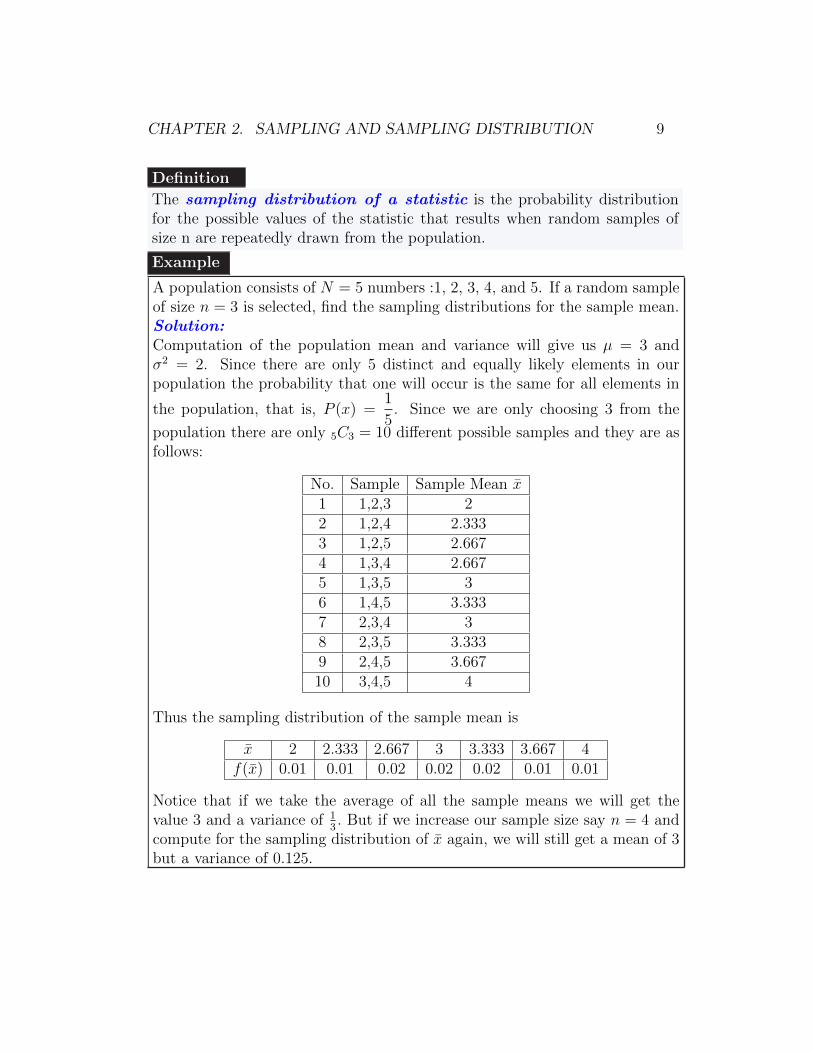
Definition

The sampling distribution of a statistic is the probability distributionfor the possible values of the statistic that results when random samples ofsize n are repeatedly drawn from the population.

Example

A population consists of N = 5 numbers :1, 2, 3, 4, and 5. If a random sampleof size n = 3 is selected, find the sampling distributions for the sample mean.Solution:Computation of the population mean and variance will give us µ = 3 andσ2 = 2. Since there are only 5 distinct and equally likely elements in ourpopulation the probability that one will occur is the same for all elements in

the population, that is, P (x) =1

5. Since we are only choosing 3 from the

population there are only 5C3 = 10 different possible samples and they are asfollows:

No. Sample Sample Mean x1 1,2,3 22 1,2,4 2.3333 1,2,5 2.6674 1,3,4 2.6675 1,3,5 36 1,4,5 3.3337 2,3,4 38 2,3,5 3.3339 2,4,5 3.66710 3,4,5 4

Thus the sampling distribution of the sample mean is

x 2 2.333 2.667 3 3.333 3.667 4f(x) 0.01 0.01 0.02 0.02 0.02 0.01 0.01

Notice that if we take the average of all the sample means we will get thevalue 3 and a variance of 1

3. But if we increase our sample size say n = 4 and

compute for the sampling distribution of x again, we will still get a mean of 3but a variance of 0.125.


Remark

We can notice that µx the mean of the sample means is equal to the popula-tion mean, and the variance σ2

x or the standard deviation σxwill decrease asour sample size increases.If all possible random samples of size n are drawn, without replacement, froma finite population of size N with mean µ and standard deviation σ, then thesampling distribution of the sample mean will be approximately normallydistributed and the mean and standard deviation is given by

µx = µ and σx =σ√n

√N − nN − 1

.

The factor√

N−nN−1

is called the finite correction factor. For large or

infinite populations , this correction factor will be approximately equal to 1.Hence σx = σ√

n

The above notion regarding the sampling distribution of the sample meangives us the foundation of the next theorem; the central limit theorem. Thecentral limit theorem states that in general situations and condition sums andmeans of samples of random observations that are drawn from a populationof any distribution tends to possess, approximately, a bell shaped distributionin repeated sampling. And thus the distribution can be assumed approxi-mately normal.

One of the significance of the central limit theorem is that it explains whysome of the observations in the real world tends to possess an approximatelya normal distribution. To illustrate this significance, consider the weight ofa person. Weight can be affected by many factors whether environmental orgenetics for instance, family lineage such as the parents weights. Anotherfactor can be the physical activities of the person. All this possibilities mayreally affect the weight of a person but the central limit theorem togetherwith other theorems applicable to the normal distribution provides an expla-nation of this events.

Another significance of the central limit theorem and probably the mostimportant attribute is its application to statistical inference. Many statis-tical estimators that are used to make inferences about a population haveparameters that are sums and averages of sample observations.


Theorem

Central Limit Theorem If random samples of size n are drawn from alarge or infinite population with mean µ and variance σ2, then the samplingdistribution of the sample mean is approximately normally distributed withmean and standard deviation

µx and σx =σ√n

where µ and sigma are the mean and standard deviation of the population,respectively.

Thus, z =x− µx(σx = σ√

n

) is a value of a standard normal random variable Z.

Remark

1. If samples are taken from a population having a normal distribution,then the sampling distribution of the sample mean will have a normaldistribution no matter what n is.

2. If samples are taken from a population which is not normally dis-tributed, then the sampling distribution of the sample mean will havean approximate normal distribution only for large samples, that is,when n ≥ 30

3. The standard deviation of the sampling distribution of x ,σx , is calledthe standard error of the sample mean .

Chapter 3Estimation

Procedures and formulas used in estimating values of unknown populationparameters that are based on information provided in a sample data are basedon the theory of sampling distributions and the methods used to collect thesesample. The sampling distributions allow us to associates specific levels ofconfidence with each statistical inference. And thus enabling us to quantifyhow much confidence we place in a sample statistic correctly estimating thepopulation parameter.

Definition

An estimator is a rule, usually expressed as a formula that tells us how tocalculate an estimate based on information in the sample.

We can classify estimators into two, point estimators and interval esti-mators.

1. Point estimation - Based on sample data, a single number is cal-culated to estimate the population parameter. The rule or formulathat describes this calculation is called the point estimator, and theresulting number is called the point estimate.

2. Interval estimation - Based on sample data, two numbers are calcu-lated to form an interval within which the parameter is expected to lie.The rule or formula that describes this calculation is called the inter-val estimator, and the resulting pair of numbers is called an intervalestimate or confidence interval.

12

CHAPTER 3. ESTIMATION 13

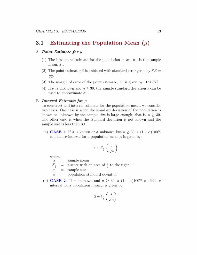
3.1 Estimating the Population Mean (µ)

A. Point Estimate for µ

(1) The best point estimate for the population mean, µ , is the samplemean, x .

(2) The point estimator x is unbiased with standard error given by SE =σ√n.

(3) The margin of error of the point estimate, x , is given by±1.96SE.

(4) If σ is unknown and n ≥ 30, the sample standard deviation s can beused to approximate σ.

B. Interval Estimate for µTo construct and interval estimate for the population mean, we considertwo cases. One case is when the standard deviation of the population isknown or unknown by the sample size is large enough, that is, n ≥ 30.The other case is when the standard deviation is not known and thesample size is less than 30.

(a) CASE 1: If σ is known or σ unknown but n ≥ 30, a (1 − α)100%confidence interval for a population mean,µ is given by:

x± Zα2

(σ√n

)where:x = sample meanZα

2= z-score with an area of α

2to the right

n = sample sizeσ = population standard deviation

(b) CASE 2: If σ unknown and n ≥ 30, a (1 − α)100% confidenceinterval for a population mean,µ is given by:

x± tα2

(s√n

)


where:x = sample meantα

2= critical t-value with an area of

α2

to the right and a degree of freedom n− 1n = sample sizes = sample standard deviation

Remark

(1) If x is used as an estimate of µ , we can then be (1− α)100% confident

that the error will not exceed Zα2

(σ√n

).

(2) If x is used as an estimate of µ , we can then be (1− α)100% confidentthat the error will not exceed a specified amount e when the sample size

is n =(Zα

2σ

e

)2

.

Example

The mean and standard deviation for the quality grade point averages of arandom sample of 36 college seniors are calculated to be 2.6 and 0.3 respec-tively. Find the 95% confidence interval for the mean of the entire senior class.Solution: The following are known:

x = 2.6, s = 0.3 , n = 36, α = 5% for a 95% C.I.

A 95% confidence interval for the quality grade point average of the entiresenior class is given by:

x± Zα2

(σ√n

)⇒ 2.6± Z 0.05

2

(0.3√

36

)⇒ 2.6± 1.96

(0.3√

36

)= (2.502, 2.698)

3.2 Estimating the Population Proportion (π)

A. Point Estimate for π

(1) The best point estimate for the population proportion,π , is the sam-ple proportion, p .

(2) The point estimator p is unbiased with standard error given by SE =√pq

n.

(3) The margin of error of the point estimate, p , is given by±1.96SE.


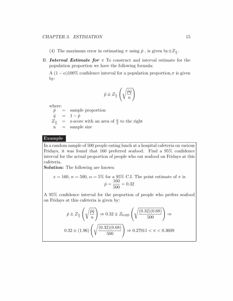
(4) The maximum error in estimating π using p , is given by±Zα2.

B. Interval Estimate for π To construct and interval estimate for thepopulation proportion we have the following formula:

A (1−α)100% confidence interval for a population proportion,π is givenby:

p± Zα2

(√pq

n

)where:p = sample proportionq = 1− pZα

2= z-score with an area of α

2to the right

n = sample size

Example

In a random sample of 500 people eating lunch at a hospital cafeteria on variousFridays, it was found that 160 preferred seafood. Find a 95% confidenceinterval for the actual proportion of people who eat seafood on Fridays at thiscafeteria.Solution: The following are known:

x = 160, n = 500, α = 5% for a 95% C.I. The point estimate of π is

p =160

500= 0.32

A 95% confidence interval for the proportion of people who prefers seafoodon Fridays at this cafeteria is given by:

p± Zα2

(√pq

n

)⇒ 0.32± Z0.025

(√(0.32)(0.68)

500

)⇒

0.32± (1.96)

(√(0.32)(0.68)

500

)⇒ 0.27911 < π < 0.3609


3.3 Estimating the Population Variance (σ2)

Suppose a sample of size n is drawn from a normal population with varianceσ2. The point estimate for the population variance,σ2, is the sample variance,s2 and a (1−α)100% confidence interval for the population variance is givenby

(n− 1)s2

χ2α2

< σ2 <(n− 1)s2

χ21−α

2

where χ2α2

and χ21−α

2are values with n − 1 degrees of freedom leaving areas

of α2

and 1− α2, respectively, to the right.

Example

The following are the volumes, in deciliters, of 10 cans of peaches distributedby a certain company: 46.4, 46.1, 45.8, 47.0, 46.1, 45.9, 45.8, 46.9, 45.2,and 46.0. Find a 95% confidence interval for the variance of all such cans ofpeaches distributed by this company, assuming that the volume is normallydistributed random variable.Solution: The following are known: n = 10, α = 0.05. We compute s2

to be 0.2934 and the chi-square values to be χ2α2

= χ20.025 = 19.023 and

χ21−α

2= χ2

0.975 = 2.700. Using these values, a95% confidence interval for the

variance of the volume of canned peaches by this company is:

(9)(0.2934)

19.023< σ2 <

(9)(0.2934)

2.700⇒ 0.2018 < σ2 < 0.5357

3.4 Errors in Estimation and Sample Size De-

termination

We note that a (1− α)100% confidence interval provides an estimate of theaccuracy of our point estimates. If the parameter is actually at the centerof the interval estimate then the “point estimate”’ estimates the parameterwithout error. However, this will not always be the case. Hence, we providethe following theorems.


Theorem

Error in Estimating µ If x is used as an estimate of µ, we can then be

(1− α)100% confident that the error will not exceed Zα2

(σ√n

).

Theorem

Sample Size for Estimating µ If x is used as an estimate of µ, we canthen be (1−α)100% confident that the error will not exceed a specified amount

e when the sample size is n =(Zα

2

σ

e

)2

.

Theorem

Error in Estimating π If p is used as an estimate of π, we can then be

(1− α)100% confident that the error will not exceed Zα2

(√pq

n

).

Theorem

Sample Size for Estimating π If p is used as an estimate of π, we canthen be (1−α)100% confident that the error will not exceed a specified amount

e when the sample size is n = Z2α2

(pq

e2

).


Exercises

1. A scientist interested in monitoring chemical contaminants in food, andthereby the accumulation of contaminants in human diets, selected a ran-dom sample of n = 50 male adults. It was found that the average dailyintake of dairy products was 756 grams per day with a standard deviationof 35 grams per day. Construct a 95% confidence interval for the meandaily intake of dairy products for men.

2. A random sample of 12 female students in a certain dormitory showedan average weekly expenditure of P400 for snack foods, with a standarddeviation of P12.50. Construct a 90% confidence interval for the averageamount spent on snack foods by female students living in this dormitory,assuming the expenditures to be normally distributed.

3. The contents of 7 similar containers of sulfuric acid are 9.8, 10.2, 10.4,9.8, 10.0, 10.2, and 9.6 liters. Find a 95% confidence interval for themean content of all such containers, assuming an approximate normaldistribution for container contents.

4. The mean and standard deviation for the quality grade point averages ofa random sample of 36 college seniors are calculated to be 2.6 and 0.3respectively. Find the 95% and 99% confidence intervals for the mean ofthe entire senior class.

5. The following data were collected based from a sample in an experiment:n = 64,x = 22.5 and s = 3.4.

(a) What is the point estimate of µ?

(b) What is the margin of error associated with the point estimate of µ?

(c) Construct a 99% confidence interval for µ.

(d) What is the maximum error of the estimate for (c)?

6. A telephone answering service completes a report in which the length ofthe call is recorded, at the end of each call. A random sample of 9 reportsyields a mean length of call of 1.2 minutes. Construct a 95% confidenceinterval for the mean length of call for the whole telephone answeringservice company if it is known that the population is normally distributedwith a standard deviation of 0.6 minutes.


7. A random sample of 10 chocolate bars has an average of 230 calories witha standard deviation of 15 calories. Assuming that the distribution of thecalories is approximately normal.

(a) Construct a 99% confidence mean calories content of this chocolatebar.

(b) How large a sample is needed if we wish to be 99% confident that oursample mean will be within 5 calories of the true mean?

8. A sample selected from a population gave a sample proportion equal to0.73

(a) Make a 99% confidence interval for π assuming n = 100.

(b) Make a 99% confidence interval for π assuming n = 600.

(c) Make a 99% confidence interval for π assuming n = 1500.

(d) Does the width of the confidence interval constructed for a-c decreaseas the sample size increases? If yes, explain why.

9. In poll of 617 workers conducted for Ernst and Young, 25% said thatthey had observed their co-workers stealing products or cash from theiremployers.

(a) What is the point estimate of the corresponding population propor-tion?

(b) What is the margin of error associated with the point estimate?

(c) Find a 95% confidence interval for the proportion of all such workerswho have observed their co-workers stealing productgs or cash fromtheir employers.

10. In a random sample of 500 teenagers 12 to 17 years old, it was found that330 have regular access to computers and the Internet.

(a) What is the point estimate of the corresponding population propor-tion?

(b) Construct a 95%confidence interval for the true proportion of teenagers12 to 17 years old who have regular access to computers and the In-ternet.


(c) What can you assert with 95% confidence about the possible size ofthe error e if you estimate the true proportion of teenagers 12 to 17years old who have regular access to computers and the Internet tobe equal to = 0.66?

11. A random sample of 985 likely voters who are likely to vote in the up-coming election were polled during a phonathon conducted by the Liberalparty. Of those surveyed, 592 indicated ha they intend to vote for theLiberal candidate in the upcoming election.

(a) Construct a 90% confidence interval for the proportion of likely votersin the population who intend to vote for a liberal candidate.

(b) What can we assert with a 90% confidence about the possible size oferror if we estimate the fraction of voters who intend to vote for theLiberal candidate is 0.601.

(c) How large a sample is needed if we want to be 90% confident that ourestimate of p is within 0.1?

Chapter 4Estimation of Two Parameters

4.1 Estimating Difference of Two Means

Let µ1 and σ1 be the mean and standard deviation, respectively, of the firstpopulation and µ2 and σ2 be the mean and standard deviation, respectively,of the second population. Random samples of size n1 are taken from thefirst population and random samples of size n2 are taken from the secondpopulation.

A. Point estimation for µ1 − µ2:

(1) The best point estimate for the difference between two populationmeans, µ1−µ2, is given by the difference between their sample means,x1 − x2 .

(2) The point estimator, x1 − x2 , is unbiased with standard error given

by SE =

√σ2

1

n1

+σ2

2

n2

.

(3) The margin of error of the point estimate is given by 1.96SE.

(4) If σ21 and σ2

2 are unknown but both n1 and n2 are 30 are more, thenthe sample variances s2

1 and s22 can be used.

B. Interval estimation for µ1 − µ2:We consider four cases in constructing a (1−α)100% Confidence Intervalfor the difference between two population means.

21

CHAPTER 4. ESTIMATION OF TWO PARAMETERS 22

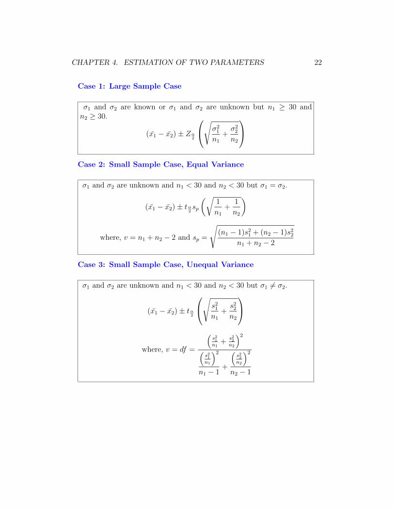
Case 1: Large Sample Case

σ1 and σ2 are known or σ1 and σ2 are unknown but n1 ≥ 30 andn2 ≥ 30.

(x1 − x2)± Zα2

√σ21

n1

+σ2

2

n2

Case 2: Small Sample Case, Equal Variance

σ1 and σ2 are unknown and n1 < 30 and n2 < 30 but σ1 = σ2.

(x1 − x2)± tα2sp

(√1

n1

+1

n2

)

where, v = n1 + n2 − 2 and sp =

√(n1 − 1)s2

1 + (n2 − 1)s22

n1 + n2 − 2

Case 3: Small Sample Case, Unequal Variance

σ1 and σ2 are unknown and n1 < 30 and n2 < 30 but σ1 6= σ2.

(x1 − x2)± tα2

√ s21

n1

+s2

2

n2

where, v = df =

(s21n1

+s22n2

)2

(s21n1

)2

n1 − 1+

(s22n2

)2

n2 − 1


Case 4: Paired Sample

σ1 and σ2 are unknown and n1 < 30 and n2 < 30 but σ1 6= σ2.

d± tαa

sd√n

where, d is the mean of the differences and sd is the standard deviation

of the differences computed as d =

n∑i=1

di

nand

sd =

√√√√√√√√√n∑i=1

d2i −

(n∑i=1

di

)2

n

n− 1

4.2 Estimating Difference of Two Proportions

Suppose independent random samples of size n1 and n2 are taken from twopopulations and let x1 and x2 be the number of successes in the first andsecond populations, respectively.

A. Point estimation for π1 − π2:

(1) The best point estimate for the difference between two populationproportion, π1 − π2, is given by the difference between their sampleproportions, p1 − p2 .

(2) The point estimator, p1 − p2 , is unbiased with standard error given

by SE =

√p1q1

n1

+p2q2

n2

.

(3) The margin of error of the point estimate is given by 1.96SE.

B. Interval estimation for π1 − π2:We consider four cases in constructing a (1−α)100% Confidence Intervalfor the difference between two population proportion.


(p1 − p2)± Zα2

(√p1q1

n1

+p2q2

n2

)

4.3 Estimating the Ratio of Two variances:σ21σ22

For any two independent random samples of size n1 and n2 selected from two

normal populations, the ratio of the sample variances,s2

1

s22

, is computed and

the following (1− α)100% confidence interval forσ21

σ22

is given by

s21

s22

1

fα2(v1, v2)

<σ2

1

σ22

<s2

1

s22

fα2(v2, v1)

where fα2(v1, v2) is an f value with a v1 = n1 − 1 and v2 = n2 − 1 degrees of

freedom leaving an area of α2

to the right.

Exercises

1. The wearing qualities of two types of automobile tires were compared byroad testing samples of 100 tires of each type. The number of miles untilwear out was defined as a specific amount of tire wear. The test resultsare given below:

Tire1 Tire2x1 = 26, 000 x1 = 25, 100

s21 = 1, 440, 000 s2

2 = 1, 960, 000

Estimate the difference in mean miles to wear out, µ1 − µ2.

2. A standardized chemistry test was given to a random sample of 50 girls and75 boys. The girls made an average grade of 76 with a standard deviationof 6 while the boys made an average grade of 82 with a standard deviationof 8. Find a 90% confidence interval for the difference µ1−µ2 where µ1 isthe mean sore of all boys and µ2 is the mean of all girls who might takethe test.


3. A course in Mathematics is taught to 12 students by the conventionalclassroom procedure. A second group of 10 students was given the samecourse by means of programmed materials. At the end of the term, thesame examination was given to each group. The 12 students meeting inthe classroom made an average group of 85 with a standard deviation of4 while the 10 students using programmed materials made an average of81 with a standard deviation of 5. Find a 90% confidence interval forthe difference between the population means, assuming the populationapproximates a normal distribution with equal variances.

4. Records for the past 15 years have shown the average rainfall in a certainregion of the country for the month of May to be 4.93 cm with a standarddeviation of 1.14 cm. A second region of the country has had an averagerainfall in May of 2.64 cm with a standard deviation of 0.06 cm duringthe past 10 years. Find a 95% confidence interval for the difference of thetrue average rainfalls in these two regions assuming that the observationscome from normal populations with different variances.

5. It is claimed that a new diet will reduce a persons weight by 4.5 kilogramson the average in a period of 2 weeks. The weights of 7 women whofollowed this diet were recorded before and after a 2-week period:

1 2 3 4 5 6 7Before 58.5 60.3 61.7 69.0 64.0 62.6 56.7After 60.0 54.9 58.1 62.1 58.5 59.9 54.4

(a) Find the average of the differences in weights before and after theweight loss program for the 4 women who participated.

(b) Find a 95% Confidence interval for the differences in weights beforeand after the weight loss program for the 4 women who participated.

(c)

6. A poll is taken among the residents of a city and the rounding countyto determine the feasibility of a proposal to construct a civic center. If2400 of 5000 city residents favor the proposal and 1200 of 2000 countyresidents favor it, find a 90% confidence interval for the true difference inthe fractions favoring the proposal to construct the civic center.


7. A geneticist is interested in the proportion of males and females in thepopulation that have a certain minor blood disorder. In a random sampleof 100 males, 24 are found to be afflicted, whereas 13 out of 100 femalestested appear to have the disorder. Compute a 99% confidence intervalfor the difference between proportion of males and females that have thisblood disorder.

8. In a study of the relationship between birth order and college success,an investigator found that 126 in a sample of 180 college students werefirstborn or only child. In a sample of 100 non-graduates of comparableage and socio-economic background, the number of firstborn or only childwas 54. Find a point estimate for the difference between the proportionsof firstborn or only child in the two populations from which these sampleswere drawn.

9. An efficiency expert wishes to determine the average time that it takes todrill 3 holes in a certain metal clamp. How large should a sample will beneeded for the expert to be 95% confident that his sample mean will bewithin 15 seconds of the true mean?

10. The government awarded grants to the agricultural departments of nineuniversities to test the yield capabilities of two new varieties of wheat.Each variety was planted on plots of equal area at each university and theyields, in kilograms per plot, were recorded as follows:

1 2 3 4 5 6 7 8 9V ariety1 38 23 35 41 44 29 37 31 38V ariety2 45 25 31 38 50 33 36 40 43

Find a 95% confidence interval for the mean difference between the yieldsof the two varieties assuming the distributions of yileds to be approxi-mately normal.

11. A random sample of 12 female students in a certain dormitory showed anaverage weekly expenditure of Php 800.00 for snack foods, with a standarddeviation of Php 175.00.

(a) What is the point estimate for the average weekly expenditure offemales in this dormitory?


(b) What is the standard error in estimating the average weekly expen-diture of females in this dormitory?

(c) Construct a 90% confidence interval for the average amount spendeach week on snack foods by female students living in this dormitory,assuming the expenditures to be approximately normally distributed.

12. Two kinds of thread are being compared for strength. Fifty pieces ofeach type of thread are tested under similar conditions. Brand A hadan average tensile strength of 78.3 kilograms with a standard deviationof 5.6 kilograms, while Brand B had an average tensile strength of 87.2kilograms with a standard deviation of 6.3 kilograms. (Use µ1 for BrandA and µ2 for Brand B )

(a) What is the point estimate for the difference in the average tensilestrength of the two threads?

(b) What is the standard error in estimating the difference of the averagetensile strength of the two kinds of thread ?

(c) Construct a 95% confidence interval for the difference of the popula-tion means.

(d) What is the maximum error in estimating the difference of the averagetensile strength of the two kinds of thread ?

13. A new rocket-launching system is being considered for deployment of smallshort-range launches. The existing system has π = 0.8 as the probabilityof a successful launch. A sample of 40 experimental launches is made withthe new system and 34 are successful.

(a) Construct a 95% confidence interval for π.

(b) Would you conclude that the new system is better? Explain youranswer.

14. A study is made to determine if a cold climate results in more studentsbeing absent from school during a semester than for a warmer climate.Two groups of students are selected at random, one group from Vermontand the other groups from Georgia. Of the 300 studnets from Vermont,64 were absent at least 1 day during the semester, and of the 400 studentsfrom Georgia, 51 were absent 1 day or more days. Find a 95% confidence


interval for the difference between the fractions of the students who areabsent in the two states.

15. A random sample of 100 homes in a certain city, it is found that 628 areheated by natural gas. Find the 98% confidence interval for the fractionof homes in this city that are heated by natural gas.

16. A random sample of 75 colleges students is selected and 16 are foundto have cars on campus. Use a 95% confidence interval to estimate thefraction of students who have cars on campus.

Chapter 5Statistical Test of Hypothesis

In a certain perspective, we can view hypothesis testing just like a jury in acourt trial. In a jury trial, the null hypothesis is similar to the jury making adecision of not- guilty, and the alternative is the guilty verdict. Here we as-sume that in a jury trial that the defendant isn’t guilty unless the prosecutioncan show beyond a reasonable doubt that defendant is guilty. If it has beenestablished that there is evidence beyond a reasonable doubt and the jurybelieves that there is enough evidence to refute the null hypothesis, the jurygives a verdict in favor of the alternative hypothesis, which is a guilty verdict.

In general, when performing hypothesis testing, we set up the null (Ho)and alternative (Ha) hypothesis in such a way that we believe that Ho is trueunless there is sufficient evidence (information from a sample; statistics) toshow otherwise.

5.1 Hypothesis Testing

A statistical hypothesis is an assertion or conjecture concerning one ormore populations.

29

CHAPTER 5. STATISTICAL TEST OF HYPOTHESIS 30

Remark

1. Null hypothesis - the hypothesis that we wish to focus our attentionon. Generally this is a statement that a population parameter has aspecified value.

• The hypothesis that is tested and the one which the researcherwishes to reject or not to reject.

• Specifies an exact value of the population parameter.

• Denoted by Ho.

2. Alternative hypothesis - the hypothesis that is accepted if the nullhypothesis is rejected.

• Allows for the possibility of several values.

• Denoted by Ha or H1.

• May be directional (quantifier < or >) or non-directional (quan-tifier is 6=).

A test of hypothesis is the method to determine whether the statisticalhypothesis is true or not. In performing statistical test of hypothesis we con-sider the following situations:

NullHypothesis

REJECTDO NOT REJECT

TRUE FALSETypeIError CorrectDecision

CorrectDecision TypeIIError

The probability of committing a TYPE I error is also called the level ofsignificance and is denoted by a small Greek symbol ”alpha”, α . Some ofthe common values used for the level of significance are 0.1, 0.05, and 0.01.For example, if α = 0.1 for a certain test, and the null hypothesis is rejected,then it means that we are 90% confident that this is the correct decision.


Remark

The following are some important properties pertaining to α and β.

• The Type I error and Type II error are related. A decrease in theprobability of one results in the increase in the porbability of the other.

• The size of the critical region, and therefore the probability of com-mitting a Type I error, can always be reduced by adjusting the criticalvalues.

• An increase in the sample size will reduce α and β simultaneously.

• If the null hypothesis is false, β is a maximum when the true value of aparameter is close to the hypothesized value. The greater the distancebetween the true value and the hypothesized value, the smaller β willbe.

Remark


The following are some important terms and concepts in performing a testof hypothesis.

1. Level of significance,α.The level of significance,α , is the probability of committing an error ofrejecting the null hypothesis when, in fact, it is true.

2. One-tailed tests v.s. Two-tailed tests.

• One Tailed Test.A one tailed test is performed when the alternative hypothesis isconcerned with values specifically below or above an exact value ofthe null hypothesis. The alternative hypothesis is directional(i.e.< or >).

• Two Tailed Test.A two-tailed test is performed when the alternative hypothesis isconcerned with values that are not equal to an exact value of thenull hypothesis. The alternative hypothesis is non-directional.

3. Test StatisticThe value generated from sample data. Test value to be compared withthe critical values.

4. Critical Region (Region of rejection/region of acceptance)

• Depends on the type of test to be performed. If test is one tailed, thenthe critical region is concentrated on either the left tail (for<) or theright tail of the distribution (for >). If test is two tailed, then thecritical region is distributed on each tail of the distribution.

• Critical values are obtained depending on the type of test to be per-formed. If the test is one tailed, the significance level will be the areaeither on the left tail or on the right tail of the distribution. If thetest is two tailed, the area in each tail of the distribution will be α

2.


The following are the steps in performing a test of hypothesis:

(1) Setup the null and alternative hypothesis.

(2) Indicate the level of significance.

(3) Determine the critical region and the corresponding critical values.

(4) Compute the value of the test statistic.

(5) Make a decision.

(6) Draw appropriate conclusion.

Bibliography

[1] R. Walpole Introduction to Statistics. Pearson Education South Asia PteLtd.2004.

[2] R. Walpole, R. Myers, K. Ye , and S. Myers Probability and Statistics forEngineers and Scientists. Pearson Education International.2007.

[3] L. Stephens Schaums’s Outline of Theory and Problems in BeginningStatistics. The McGraw-Hill Companies, Inc.1998.

[4] L. Kazmier Schaums’s Easy Outlines: Business Statistics. The McGraw-Hill Companies, Inc.2003.

[5] L. Gonick and W. Smith Cartoon Guide to Statistics. HarperCollins Pub-lisher, 1993.

[6] A. Graham Developing Thinking in Statistics Paul Chapman Publishing2006.

[7] R. Khazanie Elementary Statistics: In a World of Applications. GoodyearPublishing Inc., 1979.

34

intsta2 introductory statistics 2 -...

Documents