inventory management (session 3,4) - ximb.ac. · pdf fileinventory management (session 3,4) 1....
TRANSCRIPT
Inventory ManagementInventory Management(Session 3,4)(Session 3,4)
1
OutlineOutline
Elements of Inventory ManagementInventory Control SystemsEconomic Order Quantity ModelsThe Basic EOQ ModelThe EOQ Model with Non-Instantaneous ReceiptThe EOQ Model with ShortagesQuantity DiscountsReorder PointDetermining Safety Stocks Using Service LevelsOrder Quantity for a Periodic Inventory System
2
Elements of Inventory ManagementRole of Inventory
Inventory is a stock of items kept on hand used to meet Inventory is a stock of items kept on hand used to meet customer demand.customer demand.A level of inventory is maintained that will meet anticipated A level of inventory is maintained that will meet anticipated demand.demand.If demand not known with certainty, safety (buffer) stocks If demand not known with certainty, safety (buffer) stocks are kept on hand.are kept on hand.Additional stocks are sometimes built up to meet seasonal Additional stocks are sometimes built up to meet seasonal or cyclical demand.or cyclical demand.
3

Elements of Inventory ManagementRole of Inventory
Large amounts of inventory sometimes purchased to take Large amounts of inventory sometimes purchased to take advantage of discounts.advantage of discounts.InIn--process inventories maintained to provide independence process inventories maintained to provide independence between operations.between operations.Raw materials inventory kept to avoid delays in case of Raw materials inventory kept to avoid delays in case of supplier problems.supplier problems.Stock of finished parts kept to meet customer demand in Stock of finished parts kept to meet customer demand in event of work stoppage.event of work stoppage.
4
Elements of Inventory ManagementDemand
Inventory exists to meet the demand of customers.Inventory exists to meet the demand of customers.Customers can be external (purchasers of products) or Customers can be external (purchasers of products) or internal (workers using material).internal (workers using material).Management needs accurate forecast of demand.Management needs accurate forecast of demand.Items that are used internally to produce a final product are Items that are used internally to produce a final product are referred to as referred to as dependent demand items.dependent demand items.
Items that are final products demanded by an external Items that are final products demanded by an external customer are customer are independent demand independent demand itemsitems..
5
Elements of Inventory ManagementInventory Costs
Carrying costs Carrying costs -- Costs of holding items in storageCosts of holding items in storage..
Vary with level of inventory and sometimes with length Vary with level of inventory and sometimes with length of time held.of time held.Include facility operating costs, record keeping, Include facility operating costs, record keeping, interest, etc.interest, etc.Assigned on a per unit basis per time period, or as Assigned on a per unit basis per time period, or as percentage of average inventory value (usually percentage of average inventory value (usually estimated as 10% to 40%).estimated as 10% to 40%).
6

Elements of Inventory ManagementInventory Costs
Ordering costsOrdering costs -- costs of replenishing stock of inventory.costs of replenishing stock of inventory.Expressed as dollar amount per order, independent of Expressed as dollar amount per order, independent of order size.order size.Vary with the number of orders made.Vary with the number of orders made.Include purchase orders, shipping, handling, Include purchase orders, shipping, handling, inspection, etc.inspection, etc.
7
Elements of Inventory ManagementInventory Costs
Shortage, or stockoutShortage, or stockout costs costs -- Costs associated with Costs associated with insufficient inventory.insufficient inventory.
Result in permanent loss of sales and profits for items Result in permanent loss of sales and profits for items not on hand.not on hand.Sometimes penalties involved; if customer is internal, Sometimes penalties involved; if customer is internal, work delays could result.work delays could result.
8
Inventory Control Systems
An inventory control system controls the level of inventory by determining how much (replenishment level) and whento order.Two basic types of systems -continuous (fixed-order quantity) and periodic (fixed-time).In a continuous system, an order is placed for the same constant amount when inventory decreases to a specified level.In a periodic system, an order is placed for a variable amount after a specified period of time.
9
Inventory Control SystemsContinuous Inventory System
A continual record of inventory level is maintained.Whenever inventory decreases to a predetermined level, the reorder point, an order is placed for a fixed amount to replenish the stock.
The fixed amount is termed the economic order quantity, whose magnitude is set at a level that minimizes the total inventory carrying, ordering, and shortage costs.
Because of continual monitoring, management is always aware of status of inventory level and critical parts, but system is relatively expensive to maintain.
10
Inventory Control SystemsPeriodic Inventory System
Inventory on hand is counted at specific time intervals and an order placed that brings inventory up to a specified level.Inventory not monitored between counts and system is therefore less costly to track and keep account of.Results in less direct control by management and thus generally higher levels of inventory to guard against stockouts.System requires a new order quantity each time an order is placed.Used in smaller retail stores, drugstores, grocery stores and offices.
11

Economic Order Quantity Models
Economic order quantity, or economic lot size, is the quantity ordered when inventory decreases to the reorder point.Amount is determined using the economic order quantity (EOQ) model.Purpose of the EOQ model is to determine the optimal order size that will minimize total inventory costs.Three model versions to be discussed:
Basic EOQ modelEOQ model without instantaneous receiptEOQ model with shortages
12

Economic Order Quantity ModelsBasic EOQ Model
A formula for determining the optimal order size that minimizes the sum of carrying costs and ordering costs.Simplifying assumptions and restrictions:
Demand is known with certainty and is relatively constant over time.No shortages are allowed.Lead time for the receipt of orders is constant.The order quantity is received all at once and instantaneously.
13

Economic Order Quantity ModelsBasic EOQ Model
Figure The Inventory Order Cycle 14

Basic EOQ ModelCarrying Cost
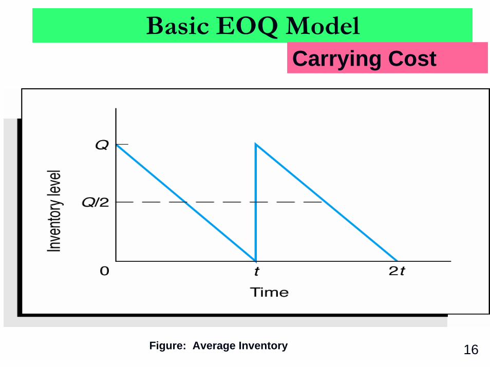
Carrying cost usually expressed on a per unit basis of time, traditionally one year.Annual carrying cost equals carrying cost per unit per year times average inventory level:
Carrying cost per unit per year = Cc
Average inventory = Q/2Annual carrying cost = CcQ/2.
15
Basic EOQ ModelCarrying Cost
Figure: Average Inventory 16
Basic EOQ ModelOrdering Cost
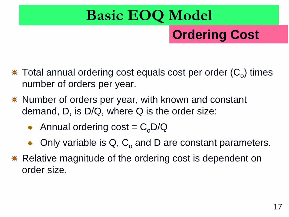
Total annual ordering cost equals cost per order (Co) times number of orders per year.Number of orders per year, with known and constant demand, D, is D/Q, where Q is the order size:
Annual ordering cost = CoD/QOnly variable is Q, Co and D are constant parameters.
Relative magnitude of the ordering cost is dependent on order size.
17
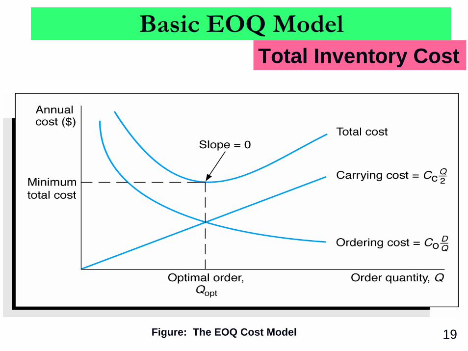
Basic EOQ ModelTotal Inventory Cost
2Q
cCQD
oCTC +=
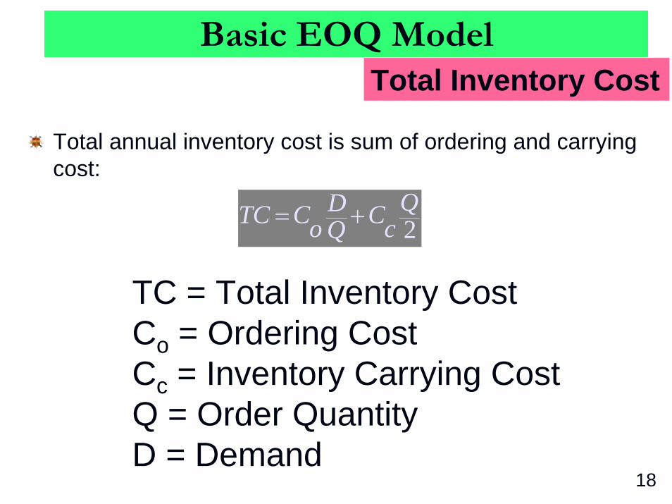
Total annual inventory cost is sum of ordering and carrying cost:
TC = Total Inventory CostCo = Ordering CostCc = Inventory Carrying CostQ = Order QuantityD = Demand
18
Basic EOQ ModelTotal Inventory Cost
Figure: The EOQ Cost Model 19

Basic EOQ ModelEOQ and Min. Total Cost
EOQ occurs where total cost curve is at minimum value and carrying cost equals ordering cost:
The EOQ model is robust because Q is a square root and errors in the estimation of D, Cc and Co are dampened.
cCDoC
optQ
optQcC
optQDoC
TC
2
2min
=
+=
20
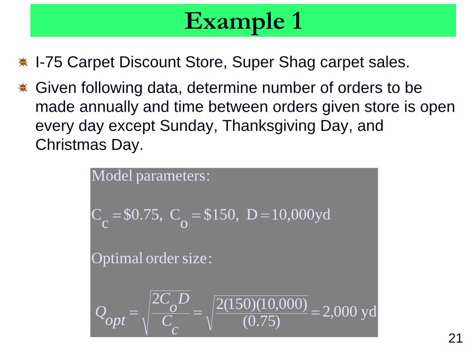
Example 1
I-75 Carpet Discount Store, Super Shag carpet sales.Given following data, determine number of orders to be made annually and time between orders given store is open every day except Sunday, Thanksgiving Day, and Christmas Day.
yd 000,2)75.0()000,10)(150(22
:sizeorder Optimal
10,000yd D $150, oC $0.75, cC
:parameters Model
===
===
cCDoC
optQ
21

days store 62.2 5311
/days 311 timecycleOrder
5000,2000,10
:yearper orders ofNumber
500,1$2)000,2()75.0(000,2
000,10)150(2min
:costinventory annual Total
===
==
=+=+=
optQD
optQD
optQcC
optQD
oCTC
22
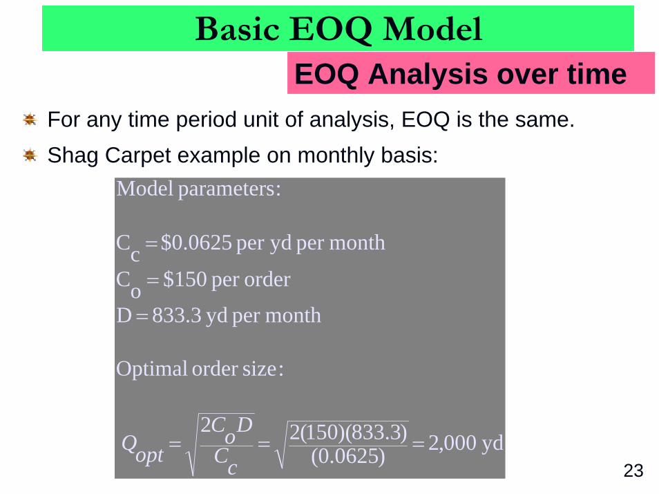
Basic EOQ ModelEOQ Analysis over time
For any time period unit of analysis, EOQ is the same.Shag Carpet example on monthly basis:
yd 000,2)0625.0()3.833)(150(22
:sizeorder Optimal
monthper yd 833.3 Dorderper $150 oC
monthper ydper $0.0625 cC
:parameters Model
===
=
=
=
cCDoC
optQ23

$1,500 ($125)(12) cost inventory annual Total
monthper 125$
2)000,2()0625.0(000,2
)3.833()150(2min
:costinventory monthly Total
==
=
+=+= optQcC
optQD
oCTC
Basic EOQ ModelEOQ Analysis over time
24

EOQ ModelNon-Instantaneous Receipt Description
In the non-instantaneous receipt model the assumption that orders are received all at once is relaxed. (Also known as gradual usage or production lot size model.)The order quantity is received gradually over time and inventory is drawn on at the same time it is being replenished.
25

EOQ ModelNon-Instantaneous Receipt Description
Figure: The EOQ Model with Non-Instantaneous Order Receipt 26
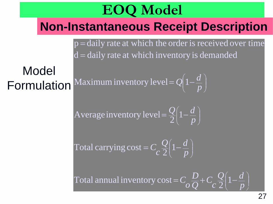
EOQ ModelNon-Instantaneous Receipt Description
⎟⎟⎠
⎞⎜⎜⎝
⎛
⎟⎟⎠
⎞⎜⎜⎝
⎛
⎟⎟⎠
⎞⎜⎜⎝
⎛
⎟⎟⎠
⎞⎜⎜⎝
⎛
−+=
−=
−=
−=
==
pdQ
cCQD
oC
pdQ
cC
pdQ
pdQ
12costinventory annual Total
12 cost carrying Total
12 levelinventory Average
1 levelinventory Maximum
demanded isinventory at which ratedaily dover timereceivedisorder heat which tratedaily p
ModelFormulation
27

EOQ ModelNon-Instantaneous Receipt Description
)/1(2
:sizeorder Optimal
curvecost totalofpoint lowest at 12
pdcCDoC
optQ
QD
oCpdQ
cC
−=
=− ⎟⎟⎠
⎞⎜⎜⎝
⎛
Equation shown above is the optimal order size under non-Instantaneous receipt
28
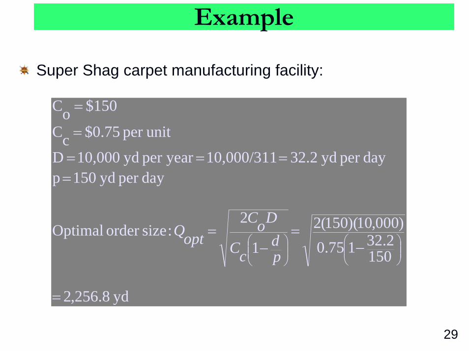
Example
Super Shag carpet manufacturing facility:
yd 8.256,2
1502.32175.0
)000,10)(150(21
2 :sizeorder Optimal
dayper yd 150 pdayper yd 32.2 10,000/311 year per yd 10,000 D
unitper $0.75 cC
$150 oC
=
−=
−=
====
=
=
⎟⎟⎠
⎞⎜⎜⎝
⎛⎟⎟⎠
⎞⎜⎜⎝
⎛pd
cC
DoCoptQ
29
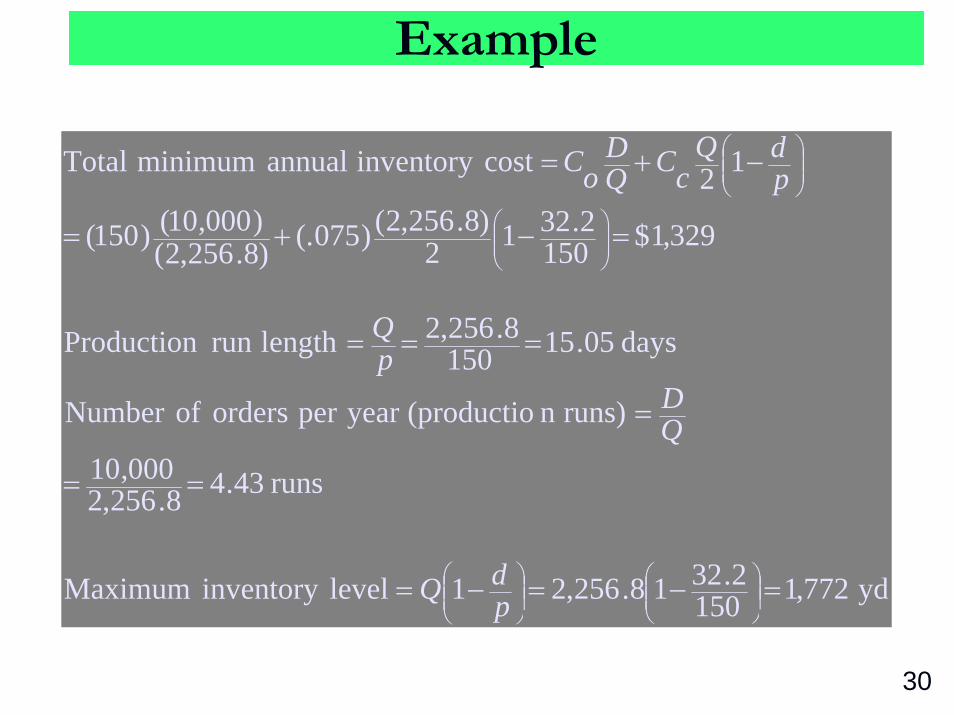
Example
yd 772,11502.3218.256,21 levelinventory Maximum
runs 43.48.256,2000,10
runs)n (productioyear per orders ofNumber
days 05.151508.256,2 length run Production
329,1$1502.3212
)8.256,2()075(.)8.256,2()000,10()150(
12costinventory annual minimum Total
=−=−=
==
=
===
=−+=
−+=
⎟⎟⎠
⎞⎜⎜⎝
⎛⎟⎟⎠
⎞⎜⎜⎝
⎛
⎟⎟⎠
⎞⎜⎜⎝
⎛
⎟⎟⎠
⎞⎜⎜⎝
⎛
pdQ
QD
pQ
pdQ
cCQD
oC
30

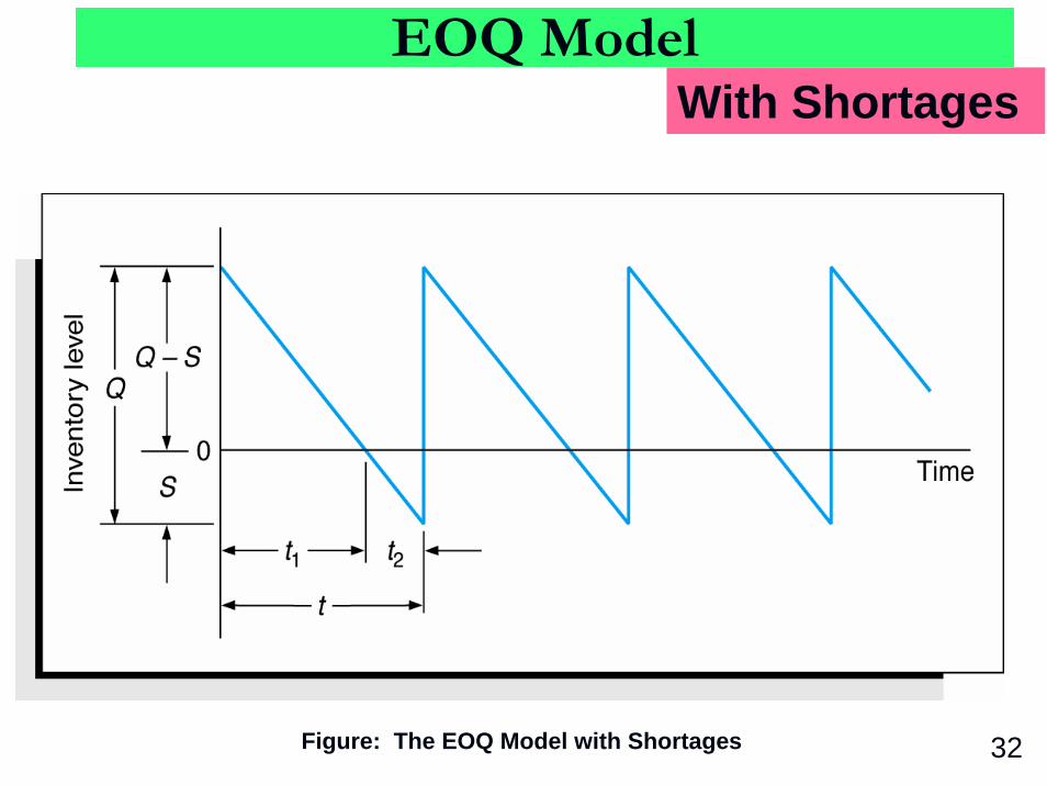
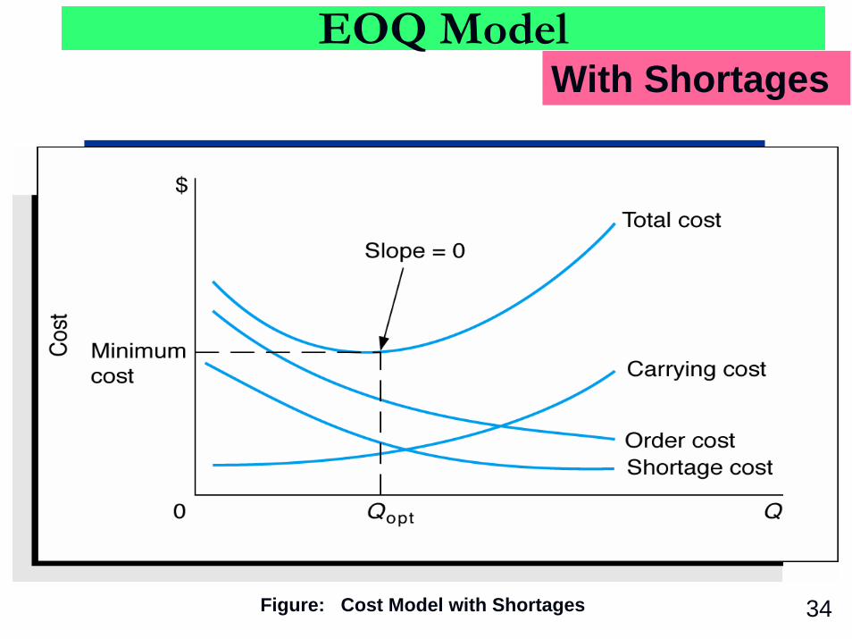
EOQ ModelWith Shortages
In the EOQ model with shortages, the assumption that shortages cannot exist is relaxed.
Assumed that unmet demand can be backordered with all demand eventually satisfied.
31
EOQ ModelWith Shortages
Figure: The EOQ Model with Shortages 32
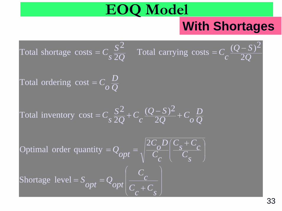
EOQ ModelWith Shortages
⎟⎟⎟
⎠
⎞
⎜⎜⎜
⎝
⎛
⎟⎟
⎠
⎞
⎜⎜
⎝
⎛
+==
+==
+−+=
=
−==
sCcCcC
optQoptS
sCcCsC
cCDoC
optQ
QD
oCQSQ
cCQS
sC
QD
oC
QSQ
cCQS
sC
level Shortage
2quantityorder Optimal
22)(
22
costinventory Total
cost ordering Total
22)( costs carrying Total 2
2 costs shortage Total
33
EOQ ModelWith Shortages
Figure: Cost Model with Shortages 34
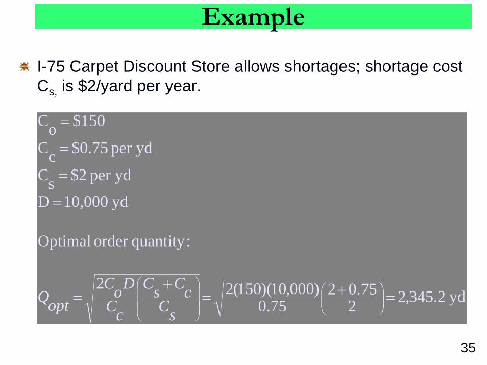
Example
I-75 Carpet Discount Store allows shortages; shortage cost Cs, is $2/yard per year.
yd 2.345,2275.02
75.0)000,10)(150(22
:quantityorder Optimal
yd 10,000 Dydper $2 sC
ydper $0.75 cC
$150 oC
=+=+
=
=
=
=
=
⎟⎟⎠
⎞⎜⎜⎝
⎛
⎟⎟⎟
⎠
⎞
⎜⎜⎜
⎝
⎛
sCcCsC
cCDoC
optQ
35

Example
$1,279.20 639.60 465.16 $174.44
2.345,2)000,10)(150(
)2.345,2(22)6.705,1)(75.0(
)2.345,2(22)6.639)(2(
22)(
22
:costinventory Total
yd 6.63975.0275.02.345,2
:level Shortage
=++=
++=
+−+=
=+=+= ⎟⎟⎠
⎞⎜⎜⎝
⎛
⎟⎟⎟
⎠
⎞
⎜⎜⎜
⎝
⎛
QD
oCQSQ
cCQS
sCTC
sCcCcC
optQoptS
36

Example
days 19.9or year 0.064 10,000639.6
D 2 t
shortage a is re which theduring Time
days 53.2or 0.17110,000639.6-2,345.2 1 t
handon isinventory which during Time
days 0.7326.4311
orders ofnumber yearper days t ordersbetween Time
yd 6.705,16.6392.345,2 levelinventory Maximum
yearper orders 26.42.345,2000,10 orders ofNumber
====
==−==
====
=−=−=
===
S
DSQ
SQ
QD
37
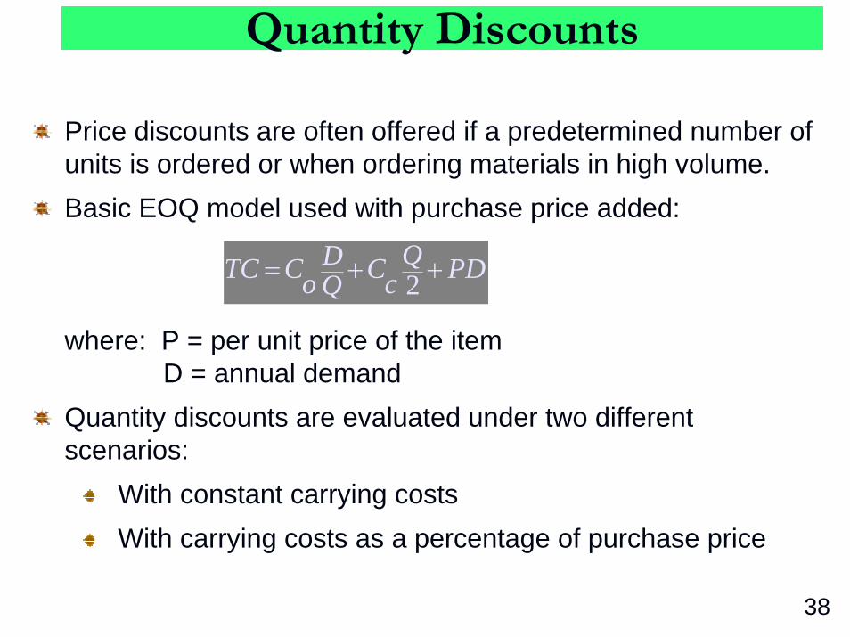
Quantity Discounts
Price discounts are often offered if a predetermined number of units is ordered or when ordering materials in high volume.Basic EOQ model used with purchase price added:
where: P = per unit price of the itemD = annual demand
Quantity discounts are evaluated under two different scenarios:
With constant carrying costsWith carrying costs as a percentage of purchase price
PDQcCQ
DoCTC ++= 2
38

Quantity Discounts with Constant Cc
Optimal order size is the same regardless of the discount price.The total cost with the optimal order size must be compared with any lower total cost with a discount price to determine which is the lesser.
39
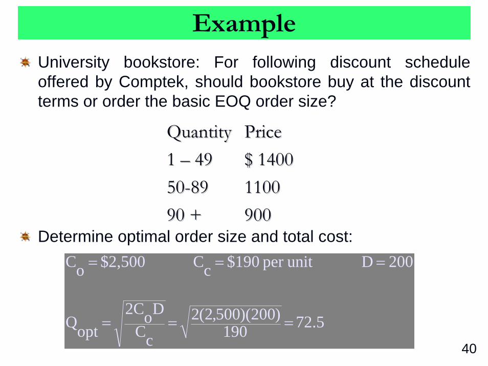
University bookstore: For following discount schedule offered by Comptek, should bookstore buy at the discount terms or order the basic EOQ order size?
Determine optimal order size and total cost:
5.72190)200)(500,2(2
cCDo2C
optQ
200D unit per $190cC $2,500 oC
===
===
Example
Quantity Quantity PricePrice1 1 –– 4949 $ 1400$ 14005050--8989 1100110090 + 90 + 900900
40
Example
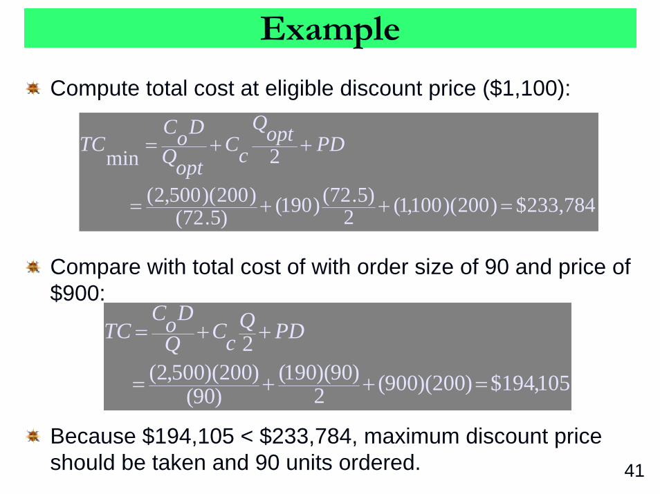
Compute total cost at eligible discount price ($1,100):
Compare with total cost of with order size of 90 and price of $900:
Because $194,105 < $233,784, maximum discount price should be taken and 90 units ordered.
784,233$)200)(100,1(2)5.72()190()5.72(
)200)(500,2(
2min
=++=
++= PDoptQcC
optQDoC
TC
105,194$)200)(900(2)90)(190(
)90()200)(500,2(
2
=++=
++= PDQcCQ
DoCTC
41

Quantity Discounts with Cc
% of Price
University Bookstore example, but a different optimal order size for each price discount.Optimal order size and total cost determined using basic EOQ model with no quantity discount.This cost then compared with various discount quantity order sizes to determine minimum cost order.This must be compared with EOQ-determined order size for specific discount price.Data:
Co = $2,500D = 200 computers per year
42

Compute optimum order size for purchase price without discount and Cc = $210:
Compute new order size:
Quantity Price Carrying Cost0 - 49 $1,400 1,400(.15) = $21050 - 89 1,100 1,100(.15) = 16590 + 900 900(.15) = 135
69210)200)(500,2(22===
cCDoC
optQ
8.77165)200)(500,2(2 ==optQ
Quantity Discounts with Cc
% of Price
43

Compute minimum total cost:
Compare with cost, discount price of $900, order quantity of 90:
Optimal order size computed as follows:
Since this order size is less than 90 units , it is not feasible,thus optimal order size is 90 units.
845,232$
)200)(100,1(2)8.77(1658.77
)200)(500,2(2
=
++=++= PDQcCQ
DoCTC
6301912009002
9013590
2005002 ,$))(())(())(,( =++=TC
1.86135)200)(500,2(2 ==optQ
Quantity Discounts with Cc
% of Price
44

Reorder Point
The reorder point is the inventory level at which a new order is placed.Order must be made while there is enough stock in place to cover demand during lead time.Formulation:
R = dLwhere d = demand rate per time period
L = lead timeFor Carpet Discount store problem:
R = dL = (10,000/311)(10) = 321.54
45

Reorder Point
Figure: Reorder Point and Lead Time 46

Reorder Point
Figure: Inventory Model with Uncertain Demand
Inventory level might be depleted at slower or faster rate during lead time.When demand is uncertain, safety stock is added as a hedge against stockout.
47

Reorder Point (4 of 4)Reorder Point
Figure: Inventory model with safety stock 48
Determining Safety Stock by Service Level
Service level is probability that amount of inventory on hand is sufficient to meet demand during lead time (probability stockout will not occur).
The higher the probability inventory will be on hand, the more likely customer demand will be met.
Service level of 90% means there is a .90 probability that demand will be met during lead time and .10 probability of a stockout.
49
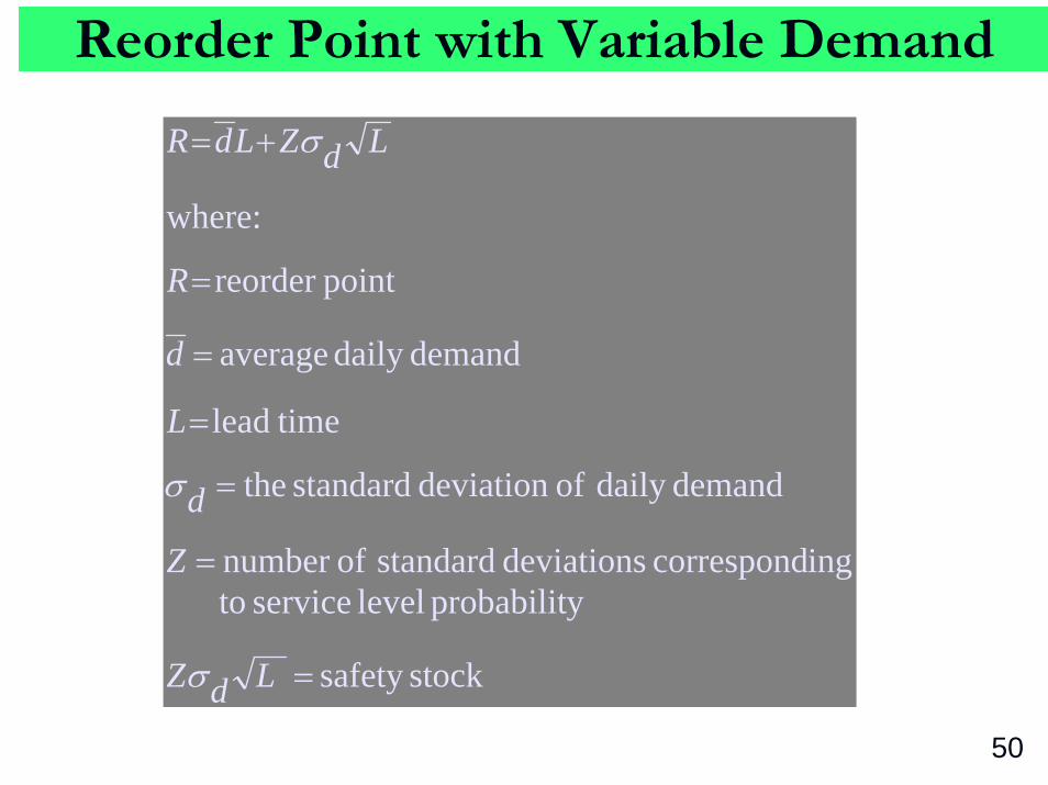
Reorder Point with Variable Demand
stocksafety
yprobabilit level service toingcorrespond deviations standard ofnumber
demanddaily ofdeviation standard the
timelead
demanddaily average
pointreorder
:where
=
=
=
=
=
=
+=
LdZ
Z
d
L
d
R
LdZLdR
σ
σ
σ
50
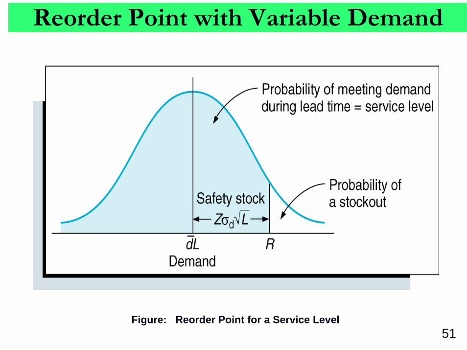
Reorder Point with Variable Demand
Figure: Reorder Point for a Service Level51
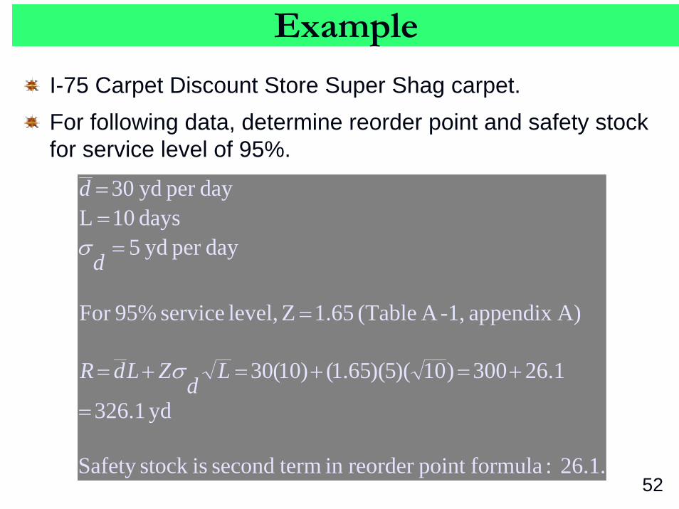
Example
I-75 Carpet Discount Store Super Shag carpet.For following data, determine reorder point and safety stock for service level of 95%.
26.1. : formulapoint reorder in termsecond isstock Safety
yd 1.326
1.26300)10)(5)(65.1()10(30
A)appendix 1,-A (Table 1.65 Zlevel, service 95%For
dayper yd 5 days 10 L
dayper yd 30
=
+=+=+=
=
===
Ld
ZLdR
d
d
σ
σ
52
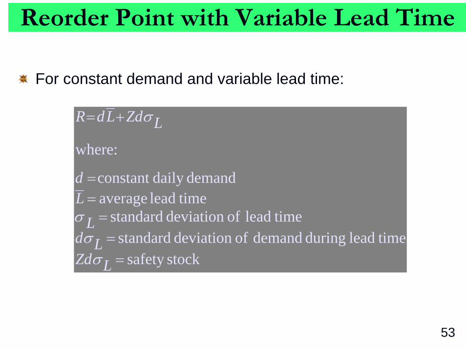
Reorder Point with Variable Lead Time
stocksafety timelead during demand ofdeviation standard
timelead ofdeviation standard timelead average
demanddaily constant
:where
===
==
+=
LZdLd
LLd
LZdLdR
σσ
σ
σ
For constant demand and variable lead time:
53
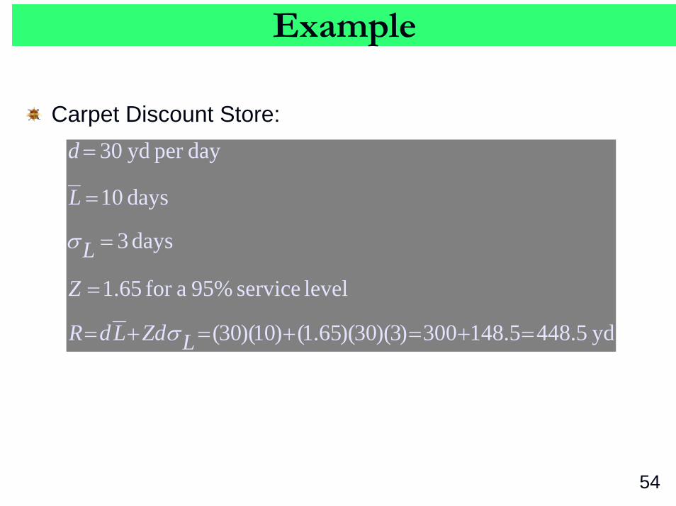
Example
yd 5.4485.148300)3)(30)(65.1()10)(30(
level service 95% afor 1.65
days 3
days 10
dayper yd 30
=+=+=+=
=
=
=
=
LZdLdR
Z
L
L
d
σ
σ
Carpet Discount Store:
54
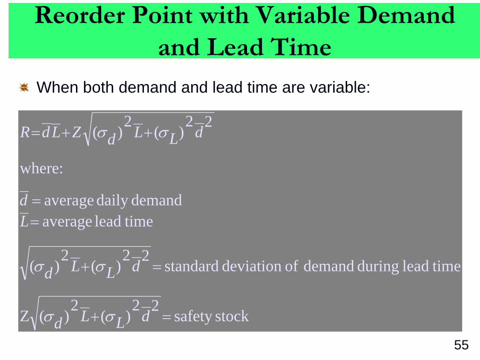
Reorder Point with Variable Demand and Lead Time
When both demand and lead time are variable:
stocksafety 22)(
2)(Z
timelead during demand ofdeviation standard 22)(
2)(
timelead average demanddaily average
:where
22)(
2)(
=+
=+
==
++=
dLLd
dLLd
Ld
dLLdZLdR
σσ
σσ
σσ
55

Example
Carpet Discount Store:
yds 450.8 150.8 300
(30)(3)(3)(30) (5)(5)(10)(1.65) (30)(10)
22)(
2)(
level service 95%for 1.65 days 3days 10
dayper yd 5 dayper yd 30
=+=
++=
++=
==
=
==
dLLdZLdR
ZL
Ld
d
σσ
σ
σ
56

Order Quantity for a Periodic Inventory System
A periodic, or fixed-time period inventory system is one in which time between orders is constant and the order size varies.Vendors make periodic visits, and stock of inventory is counted.An order is placed, if necessary, to bring inventory level back up to some desired level.Inventory not monitored between visits.At times, inventory can be exhausted prior to the visit, resulting in a stockout.Larger safety stocks are generally required for the periodic inventory system. 57
Order Quantity for Variable Demand
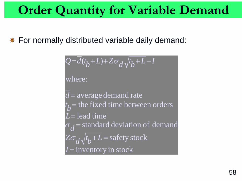
For normally distributed variable daily demand:
stockin inventory stocksafety
demand ofdeviation standard timelead
ordersbetween timefixed therate demand average
:where
)(
==+
====
−+++=
ILbtdZ
dLbtd
ILbtdZLbtdQ
σσ
σ
58

Order Quantity for Variable Demand
Corner Drug Store with periodic inventory system.Order size to maintain 95% service level:
bottles398 85 60)(1.65)(1.2 5) (6)(60
)(
level service 95%for 1.65 bottles 8 days 5
days 60 bottles 1.2
dayper bottles 6
=−+++=
−+++=
=====
=
ILbtdZLbtdQ
ZILbtd
d
σ
σ
59
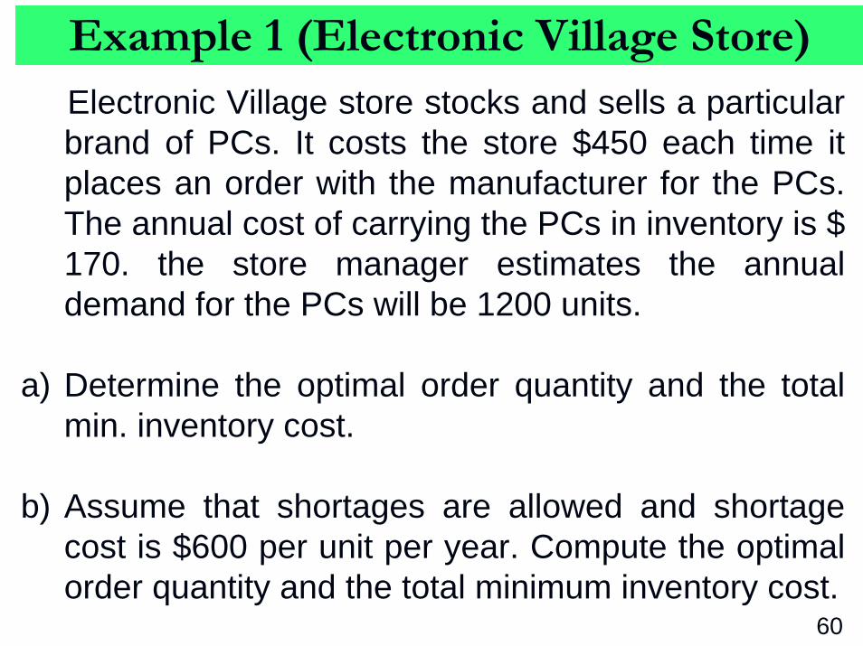
Example 1 (Electronic Village Store)Electronic Village store stocks and sells a particular brand of PCs. It costs the store $450 each time it places an order with the manufacturer for the PCs. The annual cost of carrying the PCs in inventory is $ 170. the store manager estimates the annual demand for the PCs will be 1200 units.
a) Determine the optimal order quantity and the total min. inventory cost.
b) Assume that shortages are allowed and shortage cost is $600 per unit per year. Compute the optimal order quantity and the total minimum inventory cost.
60

Example 1
For data below determine:Optimal order quantity and total minimum inventory cost.Assume shortage cost of $600 per unit per year, compute optimal order quantity and minimum inventory cost.
Step 1 (part a): Determine the Optimal Order Quantity.
computers personal 7.79170)200,1)(450(22
450$
$170 computerspersonal 1,200
===
=
==
cCDoC
Q
oCcC
D
61

Example 1
Step 2 (part b): Compute the EOQ with Shortages.
$13,549.91
7.79200,14502
7.791702cost Total
=
==+= ⎟⎟⎠
⎞⎜⎜⎝
⎛⎟⎟⎠
⎞⎜⎜⎝
⎛QD
oCQcC
computers personal 3.90
600170600
170)1200)(450(22
600$
=
+=+
=
=
⎟⎟⎠
⎞⎜⎜⎝
⎛
⎟⎟⎟
⎠
⎞
⎜⎜⎜
⎝
⎛
sCcCsC
cCDoC
Q
Cs
62

Example 1
$11,960.98
3.90200,1450)3.90(2
2)9.193.90(170)3.90(22)9.19)(600(
22)(
2
2 cost Total
computers personal 19.96001701703.90
=
+−+=
+−+=
=+=+=
⎟⎟⎠
⎞⎜⎜⎝
⎛
⎟⎟⎠
⎞⎜⎜⎝
⎛
⎟⎟⎟
⎠
⎞
⎜⎜⎜
⎝
⎛
QDoC
QSQ
cCQSsC
sCcCcC
QS
63

Example 2 (Computer Product Store)
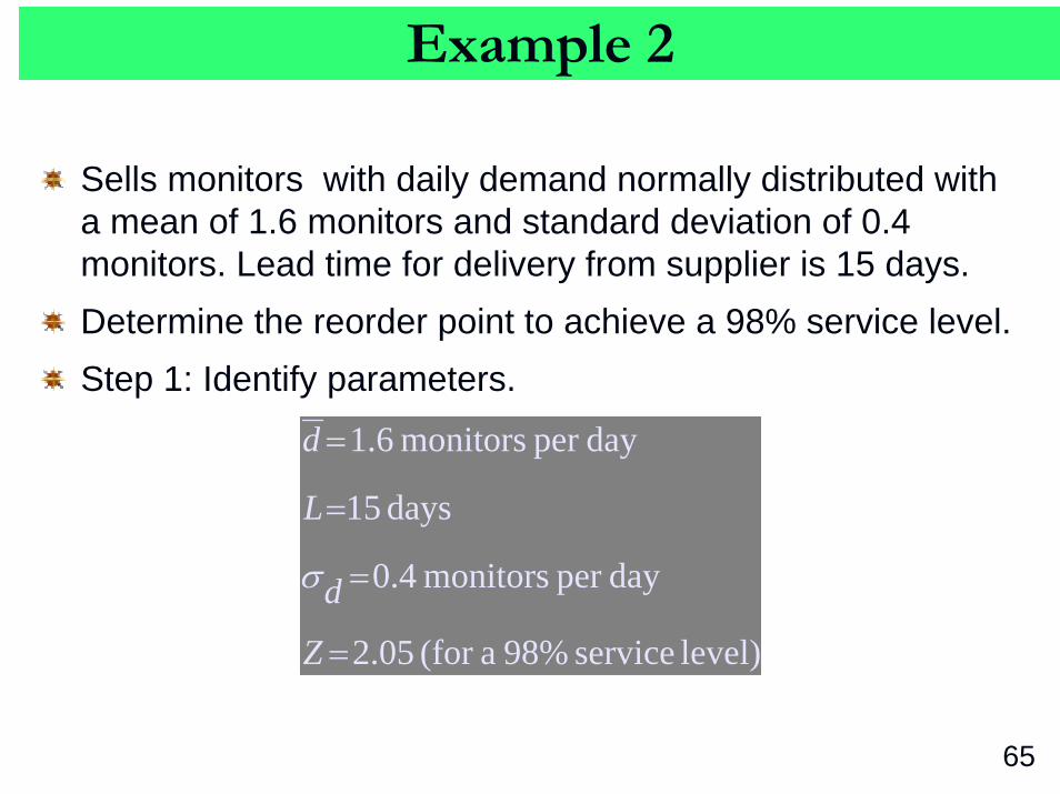
A computer products store stocks color graphics monitors, and the daily demand is normally distributed with a mean of 1.6 monitors and a standard deviation of 0.4 monitors. The lead time to receive an order from the manufacturer is 15 days.
Determine the reorder point that will achieve a 98% service level.
64
Example 2
level) service 98% a(for 05.2
dayper monitors 0.4
days 15
dayper monitors 1.6
=
=
=
=
Z
d
L
d
σ
Sells monitors with daily demand normally distributed with a mean of 1.6 monitors and standard deviation of 0.4 monitors. Lead time for delivery from supplier is 15 days.Determine the reorder point to achieve a 98% service level.Step 1: Identify parameters.
65
Example 2
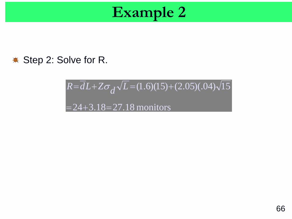
Step 2: Solve for R.
monitors18.2718.324
15)04)(.05.2()15)(6.1(
=+=
+=+= LdZLdR σ
66
ABC Classification System
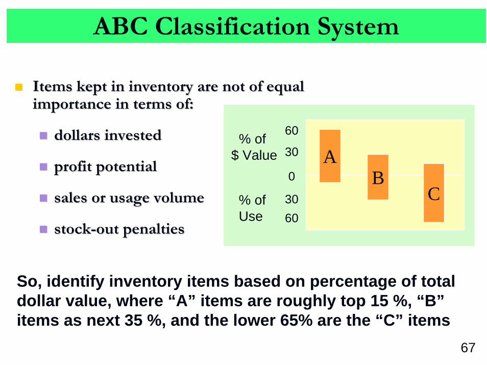
Items kept in inventory are not of equal Items kept in inventory are not of equal importance in terms of:importance in terms of:
dollars investeddollars invested
profit potentialprofit potential
sales or usage volumesales or usage volume
stockstock--out penalties out penalties
0
3060
30
60
AB
C
% of $ Value
% of Use
So, identify inventory items based on percentage of total dollar value, where “A” items are roughly top 15 %, “B”items as next 35 %, and the lower 65% are the “C” items
67
Inventory Accuracy and Cycle CountingInventory Accuracy and Cycle Counting
DefinedDefined
Inventory accuracy refers to how well the Inventory accuracy refers to how well the inventory records agree with physical inventory records agree with physical countcount
Cycle Counting is a physical inventoryCycle Counting is a physical inventory--taking technique in which inventory is taking technique in which inventory is counted on a frequent basis rather than counted on a frequent basis rather than once or twice a yearonce or twice a year
68
End of Session
69