1 © 2018 IOP Publishing Ltd Printed in the UK

Reports on Progress in Physics

S Cocco et al

Inverse statistical physics of protein sequences: a key issues review

Printed in the UK

032601

RPPHAG

© 2018 IOP Publishing Ltd

81

Rep. Prog. Phys.

ROP

10.1088/1361-6633/aa9965

3

Reports on Progress in Physics

1. Introduction

Proteins are essential in almost all cellular processes. In the course of evolution, genomic mutations cause changes in their primary amino-acid sequences. However, these changes are not completely random: only substitutions conserving the biological functionality of a protein are accepted by natural selection. Since the function of a protein relies strongly on its three-dimensional (3D) structure, also the latter has to be evo lutionary conserved. Following energy landscape theory

[1, 2], amino-acid sequences are selected such that their folded state corresponds to a deep free-energy minimum, which can be efficiently reached via a funneled free-energy landscape. We find ourselves in an apparently paradoxical situation: on the one hand, two proteins of common evolutionary ances-try (so-called homologs) may differ in more than 70 or 80% of their amino acids, but they still have highly similar three-dimensional structure and biological functions. On the other hand, even very few random mutations may destabilize a pro-tein’s fold or disrupt its biological function.

Inverse statistical physics of protein sequences: a key issues review

Simona Cocco1, Christoph Feinauer2, Matteo Figliuzzi2, Rémi Monasson3 and Martin Weigt2

1 Laboratoire de Physique Statistique de l’Ecole Normale Supérieure-UMR 8549, CNRS and PSL Research, Sorbonne Universités UPMC, Paris, France2 Sorbonne Universités, UPMC, Institut de Biologie Paris-Seine, CNRS, Laboratoire de Biologie Computationnelle et Quantitative UMR 7238, Paris, France3 Laboratoire de Physique Théorique de l’Ecole Normale Supérieure-UMR 8549, CNRS and PSL Research, Sorbonne Université UPMC, Paris, France

E-mail: martin.weigt@upmc.fr

Received 29 January 2016, revised 7 July 2017Accepted for publication 9 November 2017Published 11 January 2018

Corresponding Editor Professor Robert H Austin

AbstractIn the course of evolution, proteins undergo important changes in their amino acid sequences, while their three-dimensional folded structure and their biological function remain remarkably conserved. Thanks to modern sequencing techniques, sequence data accumulate at unprecedented pace. This provides large sets of so-called homologous, i.e. evolutionarily related protein sequences, to which methods of inverse statistical physics can be applied. Using sequence data as the basis for the inference of Boltzmann distributions from samples of microscopic configurations or observables, it is possible to extract information about evolutionary constraints and thus protein function and structure. Here we give an overview over some biologically important questions, and how statistical-mechanics inspired modeling approaches can help to answer them. Finally, we discuss some open questions, which we expect to be addressed over the next years.

Keywords: inverse problems, inverse Ising / Potts problem, statistical inference, protein sequence analysis, coevolution, protein structure prediction, protein–protein interaction

(Some figures may appear in colour only in the online journal)

Key Issues Review

IOP

2018

1361-6633

1361-6633/18/032601+17$33.00

https://doi.org/10.1088/1361-6633/aa9965Rep. Prog. Phys. 81 (2018) 032601 (17pp)

Key Issues Review

2

Over the last decades, it has been a central issue of bio-logical physics to relate the amino-acid sequence and its three-dimensional (3D) structure: in one direction, this means to solve the protein-folding problem, i.e. to determine the native 3D structure of a given sequence [1–3] . In the opposite direction, it has been asked what sequences fold into a given 3D structure, i.e. to solve the protein-design problem [4, 5]. Very precise models including the physicochemical proper-ties of amino acids and their detailled interactions have been designed and simulated [6]. While enormous progress has been made in this direction (as witnessed by the 2013 Nobel price to Karplus, Levitt and Warshel), the computational cost of realistic molecular modeling limits the length of treatable amino-acid sequences and time scales significantly.

Much more recently, an important alternative based on the progress in sequencing technology and the increasing availability of protein sequences has emerged. To date, about 70 000 complete genomes have been sequenced [7]. Instead of considering single amino-acid sequences within a detailled biophysical model, we can therefore consider entire families of homologous proteins, i.e. ensembles of diverse sequences believed to have common structure and function in different species (or different pathways inside the same species). In current databases many of these families contain more than 103 different sequences and in some cases more than 105 sequences [8]. The aim of the inverse statistical physics of proteins is to capture the sequence variability in ensembles of homologous sequences, to unveil statistical constraints act-ing on this variability, and to relate them to the conserved biological structure and function of the proteins in this fam-ily. In this sense, the inverse statistical physics of protein sequences tries to benefit from the apparent paradox between sequence variability and structural and functional conserva-tion mentioned in the first paragraph, thereby offering ideas to resolve it.

We start from a multiple-sequence alignment (MSA) of an entire protein family [9]. Note that the construc-tion of large MSA is a hard and not completely solved problem on its own, but here we assume it to be given for the sake of simplicity. An MSA is a rectangular matrix A = {aµi |i = 1, ..., L,µ = 1, ..., M}, containing M sequences, which are aligned over L positions. Each entry aµ

i of the matrix is either one of the 20 natural amino acids, or the alignment gap ‘−’ introduced to treat amino-acid insertions or deletions in some sequences. For simplicity, we will consider the gap as a 21st amino acid throughout this article, and speak about q = 21 amino acids. Each row of the MSA A is thus a single protein sequence and each column a specific position in the proteins (identifiable, e.g. via a specific location in the con-served three-dimensional protein fold).

The basic assumption of modeling this MSA using inverse methods from statistical physics [10–19] is that it constitutes a (not necessarily identically and independently distributed) sample of a Boltzmann distribution (inverse temperature β = 1 without loss of generality)

P(a1, ..., aL) =1Z exp{−βH(a1, ..., aL)} (1)

associating a probability to each full-length amino-acid sequence a = (a1, ..., aL). While this assumption is a simpli-fication of the biological reality, it will provide a useful and mathematically well-defined way to to extract information from data.

The main task of inverse statistical physics is to reconstruct the Boltzmann distribution P using a sample A drawn from P. However, in the specific situation of protein sequences this task is complicated by two opposing facts: on one side, we do not know the correct analytical form of the Hamiltonian H (e.g. in terms of local fields, two-spin or higher-order couplings etc), i.e. a priori qL − 1 free parameters are to be inferred. On the other side, even the largest MSA cover only a tiny fraction of all possible qL sequences. Parameter-reduced models have to be used in order to avoid overfitting.

We can solve these problems at least partially by assuming a specific analytical form of H and inferring the numerical val-ues of its defining parameters (e.g. local fields, pairwise cou-plings), for example by maximum likelihood. Alternatively, we can decide on a number of observables (e.g. frequencies, pair-wise correlations) whose data-derived empirical values should coincide with the thermodynamic averages in our model given by H, and use the maximum-entropy principle [20] to fix the analytical form of H. Both cases contain an important subjec-tive element: the decision on a specific model is largely driven by data availability (more data allow for more parameters) and the biological question under study. To illustrate this point, we will list a series of more and more involved questions, together with an idea about the adequate level of statistical modeling.

1.1. Homology detection and sequence annotation

Belong to the classical bioinformatic questions and are usu-ally answered using statistical models of aligned sequences [9]. Given a new natural sequence of unknown biological function, can we assign it to a known family of homologous proteins, i.e. to a given MSA? As discussed before, these fam-ilies tend to conserve important parts of the biological struc-ture and function, so the assignment of the new sequence to a previously known protein family automatically provides a prediction of its potential role in biology. Classically homol-ogy detection is done using so-called profile models, which are equivalent to independent-site Potts models in a heteroge-neous external field,

H(a1, ..., aL) = −L∑

i=1

hi(ai) . (2)

The local fields are able to capture site-specific patterns of amino-acid conservation. This may pertain to a single pos-sible amino acid in the active site of a protein (corre sponding to a column in the MSA), or to conserved physical amino-acid properties (e.g. hydrophilic amino acids in an exposed position at the protein’s surface, or hydrophobic amino acids buried inside its core). A more sophisticated version of these models, called profile Hidden Markov model [21], is able to analyze unaligned sequences and detect insertions and

Rep. Prog. Phys. 81 (2018) 032601

Key Issues Review

3

deletions while maintaining the independence of amino acids at different aligned positions.

1.2. Protein-structure prediction and the topology of coevo-lutionary networks

The assumption of independence in profile models limits the amount of information that can be extracted from an MSA since, in practice, amino acids at different positions do not evolve independently. Most single-site mutations are deleteri-ous and often perturb the physical compatibility with the sur-rounding residues in the folded protein. One may imagine that compensatory mutations in neighboring sites may repair the damage done by the first mutation; we say that residues in contact coevolve [22].

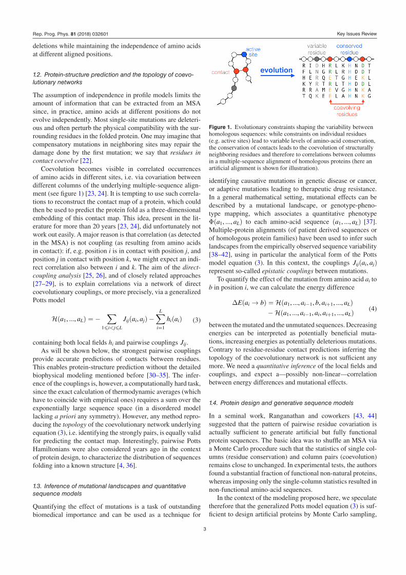
Coevolution becomes visible in correlated occurrences of amino acids in different sites, i.e. via covariation between different columns of the underlying multiple-sequence align-ment (see figure 1) [23, 24]. It is tempting to use such correla-tions to reconstruct the contact map of a protein, which could then be used to predict the protein fold as a three-dimensional embedding of this contact map. This idea, present in the lit-erature for more than 20 years [23, 24], did unfortunately not work out easily. A major reason is that correlation (as detected in the MSA) is not coupling (as resulting from amino acids in contact): if, e.g. position i is in contact with position j, and position j in contact with position k, we might expect an indi-rect correlation also between i and k. The aim of the direct-coupling analysis [25, 26], and of closely related approaches [27–29], is to explain correlations via a network of direct coevolutionary couplings, or more precisely, via a generalized Potts model

H(a1, ..., aL) = −∑

1!i<j!L

Jij(ai, aj)−L∑

i=1

hi(ai) (3)

containing both local fields hi and pairwise couplings Jij.As will be shown below, the strongest pairwise couplings

provide accurate predictions of contacts between residues. This enables protein-structure prediction without the detailed biophysical modeling mentioned before [30–35]. The infer-ence of the couplings is, however, a computationally hard task, since the exact calculation of thermodynamic averages (which have to coincide with empirical ones) requires a sum over the exponentially large sequence space (in a disordered model lacking a priori any symmetry). However, any method repro-ducing the topology of the coevolutionary network underlying equation (3), i.e. identifying the strongly pairs, is equally valid for predicting the contact map. Interestingly, pairwise Potts Hamiltonians were also considered years ago in the context of protein design, to characterize the distribution of sequences folding into a known structure [4, 36].

1.3. Inference of mutational landscapes and quantitative sequence models

Quantifying the effect of mutations is a task of outstanding biomedical importance and can be used as a technique for

identifying causative mutations in genetic disease or cancer, or adaptive mutations leading to therapeutic drug resistance. In a general mathematical setting, mutational effects can be described by a mutational landscape, or genotype-pheno-type mapping, which associates a quantitative phenotype Φ(a1, ..., aL) to each amino-acid sequence (a1, ..., aL) [37]. Multiple-protein alignments (of patient derived sequences or of homologous protein families) have been used to infer such landscapes from the empirically observed sequence variability [38–42], using in particular the analytical form of the Potts model equation  (3). In this context, the couplings Jij(ai, aj) represent so-called epistatic couplings between mutations.

To quantify the effect of the mutation from amino acid ai to b in position i, we can calculate the energy difference

∆E(ai → b) = H(a1, ..., ai−1, b, ai+1, ..., aL)

−H(a1, ..., ai−1, ai, ai+1, ..., aL) (4)

between the mutated and the unmutated sequences. Decreasing energies can be interpreted as potentially beneficial muta-tions, increasing energies as potentially deleterious mutations. Contrary to residue-residue contact predictions inferring the topology of the coevo lutionary network is not sufficient any more. We need a quantitative inference of the local fields and couplings, and expect a—possibly non-linear—correlation between energy differences and mutational effects.

1.4. Protein design and generative sequence models

In a seminal work, Ranganathan and coworkers [43, 44] suggested that the pattern of pairwise residue covariation is actually sufficient to generate artificial but fully functional protein sequences. The basic idea was to shuffle an MSA via a Monte Carlo procedure such that the statistics of single col-umns (residue conservation) and column pairs (coevolution) remains close to unchanged. In exper imental tests, the authors found a substantial fraction of functional non-natural proteins, whereas imposing only the single-column statistics resulted in non-functional amino-acid sequences.

In the context of the modeling proposed here, we speculate therefore that the generalized Potts model equation (3) is suf-ficient to design artificial proteins by Monte Carlo sampling,

Figure 1. Evolutionary constraints shaping the variability between homologous sequences: while constraints on individual residues (e.g. active sites) lead to variable levels of amino-acid conservation, the conservation of contacts leads to the coevolution of structurally neighboring residues and therefore to correlations between columns in a multiple-sequence alignment of homologous proteins (here an artificial alignment is shown for illustration).

Rep. Prog. Phys. 81 (2018) 032601

Key Issues Review

4

while the profile model equation (2) is not. For this to be true, the inferred model needs to be generative. This means that the model must not only reproduce perfectly the empirical single- and pair-column statistics (within the possibilities of the fitting algorithm), but should generate sequences that are indistinguishable from the natural sequences also in higher-order characteristics, which are not explicitly fitted using equation  (3). The above mentioned results [43, 44] suggest that this can be actually achieved using models including only local fields and pairwise couplings, while fields on their own are insufficient. Analogous ideas have been presented in [45] in the context of rewiring protein–protein interactions.

2. Statistical physics of the inverse Potts problem

We start from data given as a multiple-sequence align-ment A = {aµi |i = 1, ..., L,µ = 1, ..., M}, which contains M sequences of aligned length L. We model the statistical vari-ability in these data using generalized Potts models defined in equations (2) or (3). In this section we will provide some background on the underlying inference methodology that connects data and model, in particular on how to infer the model parameters (local fields hi(a) and couplings Jij(a, b)). A more exhaustive methodological review was recently pro-vided in [19].

This methodology will allow us to infer a specific model for each family of homologous proteins. The corre sponding MSA are freely available in public data bases, such as Pfam [8].

2.1. From data to empirical amino-acid frequencies

The statistical modeling of protein sequences relies on the fit-ting of the empirical low-order statistics of the MSA A, where each row is a protein sequence, and each column a specific aligned residue position in the proteins. In particular we esti-mate the frequencies of the occurrence of single amino acids a in the MSA column i, and of the co-occurrence of amino acids a and b in columns i and j inside the same protein:

fi(a) =1

Meff

M∑

m=1

wm δa,ami,

fi,j(a, b) =1

Meff

M∑

m=1

wm δa,amiδb,am

j,

(5)

with δa,b = 1 being the Kronecker symbol, which equals one if amino acids a and b are equal, and zero otherwise.

Note that in the sum we have introduced a sequence-specific weight wm, as well as the effective sequence number Meff =

∑m wm [26]. The reason is that sequences in an MSA

cannot be considered as independent configurations drawn from the statistical model P. The MSA collects homologous sequences that have a common ancestry. This ancestry is often relatively recent, and as a consequence sequences can be atypically similar to each other because there was no time for them to evolve further apart. While this similarity can be

used to reconstruct the evolutionary history (i.e. the phyloge-netic tree) of these sequences [46], in terms of probabilistic modeling it is a sampling bias introducing correlations not related to the structure and function of the proteins. A further bias results from the uneven selection of sequenced species—species close to model species or important pathogens tend to be more frequently sequenced than species without any direct scientific or biomedical interest.

While a proper removal of this bias remains an important open question, it can be counterbalanced by reducing the weight wm of similar sequences in the empirical frequency counts in equation (5). In a commonly used definition of the weights in the context of residue-contact prediction, wm equals to the inverse of the number of sequences aℓ of Hamming dis-tance dH(aℓ, am) (number of positions with distinct amino acids) smaller than xL. It has been shown that x ≃ 0.2− 0.3 leads to accurate and robust results. Note that ℓ = m has to be counted, too, so the weight for an isolated sequence is wm = 1, while it is smaller for any close-to-repeated sequence [26].

The empirical frequencies of equations (5) allow for quanti-fying the level of correlation between the amino-acid occu-pancies of any pair of positions (i, j). The mutual information

MIij =∑

a,b

fij(a, b) logfij(a, b)

fi(a) fj(b). (6)

is zero if and only if sites i and j are statistically independent, and positive else. It might be tempting to use the mutual infor-mation as a simple proxy for pairwise couplings. However, in the context of proteins this leads to inaccurate results since correlations emerge from networks of couplings. Inverse methods are needed to disentangle direct couplings from indi-rect correlations.

2.2. From amino-acid frequencies to Potts models

After extracting the empirical statistics from the MSA we can use it to estimate the parameters of the Potts model. This means enforcing the model to reproduce the relevant empiri-cal statistics, which can be only the first-order statistics given by the fi(a) in the independent-site case or the second-order statistics given by the fij(a, b) in the case of a pairwise Potts model. The latter constraints lead to a model with pairwise couplings Jij(a, b). This is expected to be more realistic, but comes at a high computational cost since exact inference requires the calculation of thermodynamic averages and thus the partition function Z as a sum over an exponential number qL of amino-acid sequences a = (a1, ..., aL). In this subsection we will ignore this technical difficulty, discussing the general setting of inverse Potts models. We leave the question of effi-cient approximations to the next subsection.

2.2.1. The independent-site case (IND). In the profile case of equation (2), all positions in the model distribution P are inde-pendent from each other and the joint probability is factorized over positions. We can therefore easily fit the fields hi(a) to satisfy

Rep. Prog. Phys. 81 (2018) 032601

Key Issues Review

5

fi(a) =ehi(a)

∑b ehi(b) (7)

for all positions i = 1, ..., L and all amino acids a. This equation  can be, up to a constant, easily inverted through hi(a) = ln fi(a) + const. To avoid fields to become (minus) infinite in the case of unobserved amino acids, a regular-ization or a pseudocount can be introduced, see below. This model will not reproduce the second-order statistics fij(a, b) and the probability of co-occurrence of amino acids a and b in the positions i and j is equal to fi(a) fj(b) in the model distribution.

2.2.2. Inference of pairwise Potts models. The parameters of the pairwise model equation (3), the local fields hi(a) and the couplings {Ji,j(a, b)}, have to be inferred in such a way that first and second moments of the Boltzmann distribution P correspond to the empirical frequencies. The following equa-tions have to be satisfied,

fi(a) = ⟨δa,ai⟩Pfi,j(a, b) = ⟨δai,aδaj,b⟩P (8)

for all i, j, a, b. This ensures that the marginal single- and two-site frequencies of the Potts model are equal to the empirical frequency counts derived from the original data set. In this equation, ⟨·⟩P denotes the average over the Boltzmann distri-bution P in equation (1):

⟨O(a)⟩P ≡∑

aP(a)O(a) (9)

for any observable O(a) depending on the amino-acid sequence a = (a1, ..., aL). The Np = Lq + L(L−1)

2 q2 equations  in equa-tions (8) are coupled and have to be solved simultaneously.

2.2.3. Overparametrization and gauge invariance. Note that equations  (8) are not independent. As each site i car-ries one amino acid a, the frequencies fi(a) sum up to one. Hence there are only L(q− 1) independent one-point fre-quencies. Similarly, for each one of the L(L−1)

2 pairs i, j, only (q− 1)2 pairwise frequencies fij(a, b) are independent, as marginalizing over b allows us to recover the single-site frequencies:

∑b fij(a, b) = fi(a). The number of indepen-

dent constraints coming from equation  (8) is therefore only Nc = L(q− 1) + L(L−1)

2 (q− 1)2.The number of parameters, hi(a) and Jij(a, b), defin-

ing Hamiltonian H in equation (3) equals Np and, therefore, exceeds the number of independent equations in equation (8). This overparametrization gives rise to the following gauge invariance: the probability P(a) remains unchanged under the (gauge) transformation

Jij(a, b)← Jij(a, b) + Kij(a) + Kji(b),

hi(a)← hi(a) + gi −∑

j( ̸=i)

(Kij(a) + Kji(a)

).

(10)

Here, Kij(a) and gi are arbitrary quantities. Note that Kij(a) and Kji(b) are not independent since any (ij)-dependent quanti ty

added to the first and subtracted from the second leaves the transformation invariant. The total number of independent parameters defining the above transformation equals therefore Nq = L + L(L−1)

2 × (2q− 1).Since each gauge transformation leaves the Boltzmann dis-

tribution P unchanged, the number of parameters to be fitted to the empirical data actually reduces to Np − Nq. This equals the number Nc of independent equations in equations (8), and the inference problem is well defined once the gauge is fixed. Two widely used gauges are:

• The lattice-gas gauge, in which hi(q) = Jij(a, q) =Jij(q, a) = 0 for all i, j, a, measures all energies with respect to the ‘empty’ configuration (q, ..., q), and con-siders q− 1 different ‘particle’ types a = 1, ..., q− 1.

• The zero-sum gauge (or Ising gauge) assumes that ∑a hi(a) =

∑a Jij(a, b) = 0 for all i, j, b. This gauge

generalizes the well-known case of Ising models (Jij(si, sj) = Jijsisj, hi(si) = hisi, si,j = ±1) to q-state Potts spins. Contrary to the lattice-gas gauge above, this gauge does not arbitrarily break the symmetry between the q states of the Potts variables.

As is the case with standard Ising and lattice-gas models, the two formulations are related through a simple (gauge) trans-formation of the underlying local variables, and are therefore equivalent.

2.2.4. Cross-entropy minimization and Bayesian interpreta-tion. In this section we rewrite the inverse problem in equa-tions (8) in a simpler and more interpretable way. We introduce the cross entropy

Sc({h, J}) = − 1Meff

∑

m

wm logP(am1 , am

2 , ..., amL )

= logZ −∑

i,a

hi(a) fi(a)

−∑

i<j,a,b

Jij(a, b) fij(a, b) .

(11)

This quantity gives—up to an additive P-independent con-stant equal to the entropy of the empirical distribution f (a1, ..., aL) =

∑m wm

∏i δai,am

i of the sequences in the

MSA—the Kullback–Leibler (KL) divergence

DKL( f∥P) =∑

af (a) log f (a)

P(a) (12)

between the empirical distribution f (of which fi(a) and fij(a, b) are marginals) and the Boltzmann distribution P. Within the class of pairwise Potts models defined by equa-tion  (3), a possible parameter choice is the one minimizing DKL and, hence, the cross entropy Sc. It is easy to check that the minimization with respect to fields hi(a) and couplings Jij(a, b) leads back to equations  (8). Note that the Hessian matrix of Sc is nonnegative. Zero eigenvalues correspond to directions in which the cross entropy has a minimum for parameters going to (minus) infinity; they make regularization necessary as explained in the next section.

Rep. Prog. Phys. 81 (2018) 032601

Key Issues Review

6

After minimization, the cross entropy Sc becomes a func-tion of the empirical one- and two-point amino-acid fre-quencies; more precisely it is the Legendre transform of the negative free energy logZ . The Potts parameters (fields, couplings) act as conjugated parameters to observables (one- and two-point frequencies), in the same way as pressure or chemical potential are conjugated to volume and number of particles in thermodynamical statistical ensembles. One of the basic properties of Legendre transforms is that the derivative of the potential with respect to its control parameters leads to the conjugate parameters.

Minimizing of the cross entropy is equivalent to maximiz-ing the log-likelihood in a Bayesian framework. Bayes’ theo-rem in fact allows one to express the posterior probability of the model parameters given the data, P({h, J}|{am}), starting from the probability of the data given the model, P({am}|{h, J}):

P({h, J}|{am}) = P({am}|{h, J}) P0 ({h, J})P({am}) , (13)

where P0 is a prior distribution over the Potts model param-eters. When the prior is uniform and the sequences are inde-pendently drawn from P, maximizing the posterior distribution over all couplings and fields is equivalent to minimizing the cross entropy Sc with uniform weights wm = 1

M. In the pres-ence of a non-uniform prior a term − logP0({h, J}) is added to the cross entropy, which plays the role of a regularization for the Potts parameters. In the example of a Gaussian prior P0, this penalty term is equivalent to a L2 regularization, see next subsection.

2.2.5. Regularization. Typical proteins (or protein domains, which constitute the alignable modules mak-ing a protein) have a length of L ≃ 50− 500. This leads to Nc ≃ 5 · 105 − 5 · 107 parameters to be inferred. Combined with limited sampling (M ≃ 102 − 105 for typical MSA), this large number of parameters makes regularization to avoid overfitting necessary.

Consider as an illustration the case of two amino acids, a and b, that are rarely encountered on their respective sites i and j. Assuming their frequencies to be fi(a) = fj(b) = 0.01 (note that the average frequency of amino acids is 1/q ≃ 0.048) and that they evolve independently from each other, the prob-ability of finding both amino acids in a sequence is equal to 0.0001. For MSAs with less than 10 000 sequences, such a sequence is typically not encountered. This results in an apparent anticorrelation, and ultimately, an infinitely nega-tive coupling between the two sites and amino acids. On the contrary, if the combination is found in a single out of much less than 10 000 sequences, it will lead to a large positive but statistically unsupported coupling.

To avoid such sampling effects, various regularization schemes can be used. In practice, a penalty ∆Sc({h, J}) is added to the cross entropy (11) during the minimization of the parameters {h, J}. Standard examples are the L1 norm, where

∆SL1c ({h, J}) = γ1

∑

i,a

|hi(a)|+ γ2∑

i<j,a,b

|Jij(a, b)| . (14)

The non-analyticity in zero penalizes small fields and cou-plings, forcing them to become exactly zero in value and thus favors sparse networks to be inferred. The L2 norm,

∆SL2c ({h, J}) = γ1

∑

i,a

hi(a)2 + γ2∑

i<j,a,b

Jij(a, b)2, (15)

penalizes large absolute values of parameters. This is found to be efficient in the context of protein MSA since it removes the spu-riously large parameter values based on insufficient sampling.

Another frequently used procedure to limit undersampling effects consists of adding a pseudocount to the empirical one- and two-point frequencies (justifiable via a Dirichlet prior on frequency counts):

fi(a)← (1− α) fi(a) +α

q,

fij(a, b)← (1− α) fij(a, b) +α

q2 .

(16)

The introduction of a pseudocount is—up to finite-sample effects—equivalent to assuming that the MSA is extended with a fraction α/(1− α) of sequences with amino acids sampled uniformly. Regularization parameters γ1, γ2 and α should in principal vanish as the number of data increases; values for these parameters used in practice will be discussed later on. An alternative way to regularize the inference prob-lem is to reduce the number of Potts states and keep well sam-pled amino acids only, for example with frequencies larger than some threshold values. The number of Potts states then depends on the site. This can drastically reduce the number of parameters to infer, and a weaker regularization on the remaining parameters can be used.

2.3. Methods of approximate inference

The convexity of the properly regularized cross entropy guar-antees the uniqueness of the minimum and the optimal param-eter values h, J . This minimum can be found by local convex optimization techniques. A problem is that calculating the averages in equations  (8) exactly requires the calculation of the partition function Z . This is in practice intractable for pro-teins with hundreds of residues since it includes a sum over all qN sequences. We therefore resort to approximation schemes to solve the inference problem [10–18]. Their relative advan-tages and disadvantages in the context of protein sequences will be discussed in the Results section.

2.3.1. Boltzmann machine learning (BM). The most straight-forward approximation to solve equations  (8) is called Boltzmann machine learning [47]. Starting from an initial guess for the values of the couplings and fields (e.g. the solu-tion of the independent-site model described above), the one- and two-point marginals of P are estimated by Monte Carlo Markov Chain (MCMC) sampling. They are then compared

Rep. Prog. Phys. 81 (2018) 032601

Key Issues Review

7

with the empirical one- and two-point frequencies, and the fields and couplings are modified according to

hi(a)← hi(a) + ϵ(

fi(a)− ⟨δai,a⟩P),

Jij(a, b)← Jij(a, b) + ϵ(

fij(a, b)− ⟨δai,a δaj,b⟩P),

(17)

where ε is a small parameter. The direction of the update fol-lows the gradient of the cross entropy Sc. In the case of suf-ficiently precise MCMC sampling and a sufficiently small ε, this iterative procedure is guaranteed to converge towards the solution of the fixed-point equations (8).

This procedure cannot be used directly due to its high com-putational cost. Efficient implementation going beyond simple gradient descent makes Boltzmann machine learning applica-ble to protein families smaller than about L = 200 [48–50]. Large-scale studies for hundreds or even thousands of protein families remains therefore out of reach.

2.3.2. Gaussian approximation. Using the lattice-gas gauge mentioned before, we can represent each Potts variable a by a (q− 1)-dimensional vector (s1, ..., sq−1) with entries sb(a) = δb,a. Amino acids a = 1, ..., q− 1 are thus represented by unit vectors in direction a, while the reference amino acid (or the gap) is represented by the zero vector (0, ..., 0). The MSA becomes a matrix of M rows and (q− 1)L columns with binary entries {0, 1}. The average of the column corre-sponding to position i, amino acid a equals the empiri-cal frequency fi(a), the (q− 1)L-dimensional covariance matrix Cij(a, b) = fij(a, b)− fi(a) fj(b), i, j = 1, ..., L, a, b = 1, ..., (q− 1).

The Gaussian approximation ignores the binary nature of the s-variables and treats them as continuous variables having the same means and covariances [29, 51]. The pairwise Potts model is transferred into a multivariate Gaussian model with parameters Jij(a, b). The cross-entropy can be calculated ana-lytically (up to a coupling-independent normalization),

SGc = −1

2log Det (−J)−

∑

i<j,a,b

Jij(a, b) Cij(a, b) . (18)

Equation (18) can be easily minimized over J, giving

Jij(a, b) = −(C−1)

ij (a, b) . (19)

The original exponential-time inference problem (time qL) is replaced by a simple inversion of the empirical covariance matrix, a task requiring ∼L3 operations. It can be achieved on a standard desktop computer even for long proteins of L ≃ 1000 amino acids.

2.3.3. Mean-field approximation (MF). The standard MF approximation allows one to estimate one-point marginals self-consistently. Plugging in equations  (8), which equate empirical and model derived frequencies, we find

fi(a)fi(q)

= exp

⎧⎨

⎩hi(a) +∑

j,b

Jij(a, b) fj(b)

⎫⎬

⎭ (20)

within the lattice-gas gauge. Covariances can be calculated using linear response, i.e. ∂Pi(a)/∂hj(b) = Cij(a, b). This

again leads to equation (19) and the couplings can be obtained by inverting the covariance matrix [10, 26]. The fields can then be obtained by resolving equations (20) with given single-site frequencies and couplings.

Together with the Gaussian approximation, MF is cur-rently the computationally most efficient approximative infer-ence scheme for the inverse Potts problem. However, it will not converge to the exact solution even with infinite data, and no rigorous bounds on inference errors are known. One can also formulate refined mean-field approximations, based on e.g. the Thouless–Anderson–Palmer or Bethe–Peierls approx-imations, but they have not found to be of advantage when applied to protein MSAs.

2.3.4. Pseudolikelihood maximization (PLM). In the PLM technique [15, 52, 53], the log probability of the data given the parameters in equation (11) is replaced by a sum of site-dependent terms:

M∑

m=1

wm logP(am1 , ..., am

L )→L∑

i=1

M∑

m=1

wm logP(ami |am

−i). (21)

Here, i denotes a site and a−i denotes the sequence a with-out the ith site. Note that the sum contains one term for each i and these terms contain probability distributions over a single amino acid (given the others). This means that for normal-izing these terms we need to calculate L individual sums over q amino acids instead of one sum over qL sequences. Setting

SPLMc (i) = −

M∑

m=1

wm logP(ami |am

−i), (22)

the cross entropy is the sum

SPLMc =

L∑

i=1

SPLMc (i) (23)

over the site-dependent terms. In terms of couplings and fields these terms can be written as

SPLMc (i) =

M∑

m=1

wm

[log

{∑

a

ehi(a)+∑

j( ̸=i) Jij(a,amj )

}

− hi(ami )−

∑

j( ̸=i)

Jij(ami , am

j )

⎤

⎦ .

(24)

While SPLMc is not an approximation for the cross-entropy

Sc, the method of minimizing SPLMc can be shown to be statisti-

cally consistent [52]: the true couplings and fields are recov-ered in the limit of infinite data if the data are indeed sampled from a pairwise Boltzmann distribution.

Interestingly, this statistical consistency remains valid if the SPLM

c (i) are minimized independently. While this allows for a parallel and efficient implementation, it leads for finite data to asymmetric couplings Jij(a, b) ̸= Jji(b, a). In practice, we infer each coupling as the mean of the asymmetric esti-mates [Jij(a, b) + Jji(b, a)]/2.

The key advantage of PLM is that the cross entropy is cal-culated from the sampled sequences, and there is therefore

Rep. Prog. Phys. 81 (2018) 032601

Key Issues Review

8

no need for an exponential-time calculation of the partition function. However, SPLM

c does not depend only on the empiri-cal single- and two-site frequencies, but on the complete set of sampled configurations. PLM becomes therefore slower for larger samples and the running time grows linearly with the number M of sequences.

2.3.5. Adaptive cluster expansion (ACE). The minimal cross entropy Sc can be formally written as a sum of 2L − 1 cluster contributions [14], each depending only on the empirical fre-quencies fi and fij of the sites inside the cluster:

SACEc =

∑

i

∆Si( fi) +∑

i<j

∆Sij( fi, fj, fij)

+∑

i<j<k

∆Sijk( fi, fj, fk, fij, fjk, fik) + . . . . (25)

Here, ∆S denotes the contribution to the cross entropy from a cluster that cannot be deduced from the contributions of all its subclusters [54]. Expansion (25) is, however, of limited use if not truncated to a small number (compared to 2L) of terms. A convenient truncation scheme is obtained by sum-ming only contributions ∆S exceeding (in absolute value) an arbitrary threshold θ, as large cluster contributions automati-cally identify groups of strongly interacting variables. In prac-tice, clusters are recursively constructed, starting from small size ones (2 sites) through progressive inclusion of sites. The process is iterated until all newly created clusters have |∆S| smaller than θ. The derivatives of SACE

c with respect to the frequencies { fi(a), fij(a, b)} give access to the Potts param-eters {hi(a), Jij(a, b)}. The threshold θ is tuned such that the inferred model reproduces the data statistics, as can be verified through Monte Carlo sampling, up to finite-sampling errors.

ACE, similarly to Boltzmann-machine learning and dif-ferently from the Gaussian, mean-field and pseudolikelihood approximations, accurately reproduces the sampled frequen-cies and correlations by construction [54, 55]. Due to the prop-erties of the inverse susceptibility (Fisher information) matrix, the convergence of the expansion depends on the structure of the interaction graph rather than on the magnitude of data cor-relation. The threshold θ acts as a regularizer: the complexity of the network is adapted to the level of sampling, in particular it will be sparse for bad sampling. The disadvantage of ACE is that it is computationally more involved than any of the other approximative methods: it requires the exact calculation of the partition function for each cluster. The computational bur-den is largely decreased by the compression of the number of Potts states to restrict the inferred model to only well observed amino acids, as described above, and by the possibility to run it in combination with Boltzmann-machine learning [55].

2.3.6. Other approaches. There are several other interest-ing methods, e.g. minimal probability flow [56] or Bayesian networks [27], which have been applied to protein sequence modelling.

3. Modeling families of protein sequences

After having adressed inverse models in statistical physics from the methodological point of view, we will give a few exemplary results from using these methodologies with real protein sequence data.

3.1. Homologous protein families and profile models

State-of-the-art techniques for homology detection and sequence alignments are based on the patterns of amino-acid conservation in individual positions [9]. A class of statistical models are independent-site profile models, which assume all positions (or columns in an alignment) to be statistically inde-pendent. In the case of unaligned sequences, profile models can be generalized to profile hidden Markov models. These combine residue conservation patterns with the possibility of identifying insertions and deletions in a sequence and are among the most successful statistical models in bioinformati-cal sequence analysis. They are at the basis of databases of homologous protein families such as Pfam. The Pfam data-base (release 28.0 in 2015) contains 16 230 protein domain families, out of which 6783 contain more than 1000 sequences [8]. This number of sequences is empirically known to be a lower bound to the size of an input MSA providing accurate and robust predictions by pairwise statistical modeling. Only 10 years ago, there were about 600 families (release 20.0 in 2006) in Pfam, and the number of accessible families contin-ues to grow quickly. Approaches from inverse statistical phys-ics that go beyond profile models can now be applied to the majority of protein families.

3.2. Potts models: accurate fitting versus topological inference

The inference of the couplings and fields of a pairwise Potts model (3) from aligned amino-acid sequences is a computa-tionally hard task. It is expected that the approximate inference methods vary in quality of the resulting predictions. Since a ‘true’ model does not exist—evolution is not a Monte Carlo simulation of a Boltzmann distribution—it is not clear how to assess the accuracy of the inferred model. A straight forward benchmark would be to check if equation (8), which equate empirical and model statistics, are well fitted. Using the pro-tein family PF00014 (Trypsin inhibitor: L = 53, M = 4915) as an example, we apply the different approaches discussed in the last section for parameter inference. Subsequently we sample artificial sequences from the inferred statistical model P(a1, ..., aL) using MCMC, in order to estimate the model sta-tistics. In figure 2 we show the results: while mean-field infer-ence [26] and pseudo-likelihood maximisation [53] reproduce the empirical statistics badly (mean-field actually leads to serious problems in equilibration MCMC simulations), BM [57] and ACE [55] are much more precise.

Rep. Prog. Phys. 81 (2018) 032601

Key Issues Review

9

Does this mean that MF and PLM are of no use for analys-ing large MSA? As argued in the introduction, the answer is not so easy. When predicting residue contacts in the three-dimensional fold of a protein, we do not need the fine sta-tistics of the empirical data to be reproduced. We need to correctly capture the topology of the network of coevolution-ary couplings.

To assess the topology, we need to map the q× q coupling matrix Jij(a, b) for each pair (i, j) onto a scalar quantity meas-uring the coupling strength between the two sites i and j. A quantity often used [53] is the Frobenius norm of the coupling matrices for each (i, j),

Fij =

√∑

a,b

Jij(a, b)2 . (26)

Since the Frobenius Norm is gauge dependent, we have to specify in which gauge we calculate it. A sensible choice is the zero-sum gauge discussed above. It minimises the Frobenius norm and explains thereby ‘as much as possible’ by fields, and ‘as little as necessary’ by pairwise couplings. Contact predic-tions improve furthermore when using the average-product correction (APC) [58]:

FAPCij = Fij −

∑k Fik

∑k Fkj∑

k,ℓ Fkℓ. (27)

This correction is identical to the measure of modularity com-monly used for describing networks [59], and amounts to sub-stracting from the Frobenius norm a null-model contribution for the pair i, j due to the single-site properties of i and j [60].

The resulting FAPC-values are highly correlated for differ-ent methods. In particular the largest values, which character-ize the sub-network of the strongest coevolutionary couplings, are found to strongly overlap. As an example, out of the top 50 coupled pairs found by BM, 80% (resp. 70% / 62%) are also within the first 50 pairs identified by PLM (resp. MF / ACE); these fractions rise to 100% (resp. 88% / 76%) if we look for these 50 top-scoring BM predictions within the first 100 PLM (resp. MF / ACE) pairings. The lower overlap between ACE and the other methods results from the weaker regulariza-tion used, which allows for a better fitting but at the cost of introducing a number of strong couplings between rare amino acids. A random selection of 50 pairs for each method would result in an mean overlap of less than 4%, illustrating the high significance of the reported overlaps.

We conclude that if the aim of the inference is the identifi-cation of pairs with substantial coevolution, then even simple and computationally efficient methods like MF and PLM can provide accurate results. If, on the contrary, model energies or probabilities have to be accurate, then more precise methods such as ACE or BM are required. This is for example the case if one wants to sample from the inferred distribution.

Figure 2. Comparison of different methods: covariances (main panels) and single-point frequencies of the model P as commpared to the empirical values resulting from the original MSA. While the Boltzmann machine (BM) is guaranteed to accurately fit the empirical values after e sufficient number of iterations of equation (17), all others are based on approximations. MF does not reproduce the empirical statistics (it actually has important ergodicity problems when sampling by MCMC), while PLM shows a clear improvement. ACE accurately fits the single-sire frequencies and large enough covariances, deviations for small covariances result from lumping together all symbols a with probabilities fi(a) < 0.05, such covariances have therefore low statistical support and large relative error, see [55]).

Rep. Prog. Phys. 81 (2018) 032601

Key Issues Review

10

Another interesting observation is reported in figure  3, which shows histograms of Hamming distances of sequences to the consensus sequence (a⋆1 , ..., a⋆

L) given by the most frequent amino acids a⋆

i = arg maxafi(a) in each column i, comparing natural sequences from the original MSA to sequences sampled from different inferred models. While the independent model IND reproduces the average distance (by definition of IND and the linearity of the Hamming distance), the histogram is visibly more concentrated than for natural sequences. PLM shows systematic deviations due to the lack of fitting accuracy, while ACE and BM accurately reproduce the empirical histograms. This is astonishing since the histo-gram measures quantities which are not fitted via the Potts model, and illustrates the capacity of statistical models with pairwise couplings to well capture the sequence variability even beyond pairwise observables.

3.3. Residue-residue contact prediction and tertiary structure

The original motivation underlying the use of Potts models for describing the sequence variability across evolutionary related proteins is the prediction of residue-residue contacts [25]. This task is considered hard but important in bioinformatics: experimental determination of protein structures (x-ray crys-tallography, NMR, cryo-electron microscopy) is expensive, time consuming, and frequently of uncertain outcome. On the

other hand, freely accessible sequence databases are growing fast. If it were possible to use such sequence data for predict-ing contacts between residues, this information could in turn help to predict protein structures (intra-protein contacts) or to assemble multi-protein complexes (inter-protein contacts). Since protein function typically relies on protein structure (e.g. via binding of other molecules to well defined interfaces on the protein surface), this would provide crucial informa-tion about the operation of the proteins and the biological pro-cesses they participate in. The validity of contact predictions is assessed by comparison with known structures of proteins belonging to the family under consideration. This structural information is complementary to the sequence data and only available for a fraction of protein families.

Within DCA, residue position pairs (i, j) are sorted accord-ing to their interaction strengths as measured by FAPC

ij . We expect the most coupled pairs to be in contact. High scores are thought to indicate compensatory mutations in neighbouring residues in a protein structure (see Introduction).

Pairs of residues i, j with short separation |i− j| along the backbone frequently possess large FAPC

ij -values. These large scores often come from the presence of stretches of gaps, and are not very much relevant as far as structural predictions are concerned. For this reasons and since long-range (along the protein backbone) contacts are more informative about the tertiary structure most predictors do not include pairs with

Figure 3. Comparison of different methods: the panels show histograms of Hamming distances of natural and model-generated sequences from the consensus sequence. The blue curves show the histograms for natural sequences (sampled from the initial MSA with frequencies proportional to the sequence weights), the orange ones for the different models (IND, PLM, ACE, BM). While IND and PLM show significant deviations, ACE and BM accurately reproduce the empirical histograms. Note that the measured distance is not fitted by the Potts model and therefore not automatically reproduced even by an accurately inferred Potts model.

Rep. Prog. Phys. 81 (2018) 032601

Key Issues Review

11

|i− j| ! 4 into the evaluation, a distance corresponding to one turn in an α-helix.

Figure 4 shows an example for this procedure. Results obtained for 4915 sequences of length 53 amino acids, all belonging to the Pfam protein family PF00014 (trypsin inhibitor), are mapped onto the corresponding x-ray crys-tal structure (PDB ID 5PTI [61]). The left panel shows that the prediction by the strongest correlations (as measured by mutual information (6)) includes a large fraction of false pos-itives (green lines). Predictions based on the strongest cou-plings, shown in the right panel, lead to a significantly better prediction (red lines).

While here we present only one example, the predictive performance has been tested for thousands of protein families [26, 35]. A consistent improvement of DCA over correlations has been shown. Interestingly, the quality of the inference has only a small impact on the contact prediction. The reason is that in order to obtain a good performance in contact predic-tion, it is sufficient to infer the topological aspects of the net-work reasonably well. While approximate methods like MF or PLM may have a larger error in the inference of the exact parameter values than more exact methods like BM or ACE, they robustly predict network topology, see the last section. In fact, PLM is currently the best stand-alone method for effi-cient contact prediction.

The observation that the strongest coevolutionary cou-plings—i.e. the strongest pairwise evolutionary constraints—correspond to residue-residue contacts can be interpreted as a sequence-data driven support for so-called structure-based models (SBM) [62, 63], which themselves are motivated by the energy landscape theory [1, 2] mentioned in the Introduction: SBM assume that the folding process is mainly guided by native residue contacts. In turn, the central use for the residue contacts extracted from MSAs with DCA is in the prediction of protein structures. While the structure of a protein is usually

defined by its amino-acid sequence (Anfinsen’s principle [64]), the general process of protein folding in vivo is not fully understood. Setting this question aside for the moment, one can also ask the easier questions on how to computationally infer the folded structure of a protein from its sequence. In the last decades, this was a central question in computational biol-ogy and many methods have been devised. Even though the performance of these methods has made impressive advances, the problem is still considered as unsolved in general [3].

In this context, DCA has been shown to provide valuable information. The predicted residue contacts can be used as prior information on the structures. Such information restricts the number of possible structures and makes the task thus eas-ier. The importance of predicted contacts in the field can be illustrated by the fact that many of the top-performing groups in the last CASP challenge (http://predictioncenter.org/) have made use of them. Hundreds of novel protein structures have been predicted using coevolutionary contact predictions [32, 35]: to this aim, global pairwise contact predictions guide the assembly of local but higher-order structural elements like secondary structures (see [31, 34]) or protein fragments (see [35]).

As a last point, we note that the best performing methods for predicting residue contacts are meta-methods. These meth-ods use other methods like DCA as input and combine them using machine-learning techniques for an improved predic-tion [65–67]. Since they use supervised learning techniques to model the input-output relation between MSA and contact map, it is not surprising that they outperform any unsuper-vised method in this task.

3.4. Predicting interaction partners and inter-protein residue contacts in protein–protein interaction

The formalism of Potts models and DCA can be used to extract biological information on different scales. While we focused above on how to infer contacts between residues within a pro-tein, we now describe how to use the same formalism to infer interactions between proteins [68, 69]. When extended to all proteins in a genome, this can then be used to infer an organ-ism-wide protein–protein interaction network.

The model in equation  (3) defines a probability P(a) for finding sequence a for a specific protein belonging to pro-tein family A in an organism. We now define a probability P(a, b) for finding sequence a for a protein belonging to fam-ily A and sequence b for a protein belonging to family B in the same organism. The general idea is that if the members of the two protein families interact in all or most organisms, they have to be mutually compatible. Therefore, one would expect P(a, b) ̸= P(a)P(b) in such cases.

An intuitive extension of equation  (3) for two protein sequences a and b is

H(a, b) = HA(a) +HB(b) +HAB(a, b),

where HA(a) and HB(b) are of the form of equation (3) and model the coevolution between residues within the proteins A and B. The additional interaction term

Figure 4. Residue-residue contact prediction based on ranking of correlations (left) and Potts couplings (right) for the PF00014 protein family (trypsin inhibitor). Top 30 values of the mutual information (i.e. correlations) and FAPC (i.e. couplings) scores are mapped onto the protein structure (PDB ID: 5PTI), excluding trivial predictions with separation |i− j| ! 4 along the amino-acid sequence. Red bars correspond to residue pairs in contact (distance below 8Å, true positives), green bars to distant residue pairs (false positives). Inference was done using the mean-field approximation.

Rep. Prog. Phys. 81 (2018) 032601

Key Issues Review

12

HAB(a, b) = −La∑

i=1

Lb∑

j=1

Jij(ai, bj)

contains LaLbq2 coupling parameters, with La and Lb being the length of the sequences a and b. These parameters describe the coevolution between residue pairs in different proteins.

The model including the interaction term defines a prob-ability for a pair of sequences in the same organism. As data for the inference process we therefore need two MSAs, one for protein family A and one for protein family B. We then search for pairs of sequences (one from A and one from B) that come from the same organism and treat their concatenation as a single configuration of the composed Potts model.

A problem can arise when there are several sequences belonging to the same protein family inside a single organ-ism (such sequences are called paralogs). The problem which sequences to pair in such cases is called matching and can be solved either by biological prior information [68, 69] or by another layer of probabilistic modeling [70, 71].

As an interaction score for residue pairs between two pro-teins the FAPC scores of equation  (27) can be used. A pos-sible interaction score for two proteins is then the average of the n largest FAPC scores between the proteins. It has been shown that n = 4 gives a good performance, since it takes into account the strongest signals, but averages over a few pairs to be less susceptible to noise.

In figure  5 we represent as an example the inference results for the two ribosomal subunits. The units consists of 49 proteins and within the experimentally determined struc-ture (PDB: 2Z4K, 2Z4L [72]) 50 pairs are interacting, i.e. only 8.4% out of the 596 intra-unit protein pairs. We use the approach outlined above to fit a Potts model to each of the corresponding 596 protein-family pairs and calculated inter-action scores with n = 4. Of the ten pairs with the largest interaction scores in each unit, 16 are interacting in the struc-ture, covering most pairs with large interaction interfaces (i.e. fat lines in the figure). This predictive precision of 80% has to be compared with the 8.4% to be expected on average in a random prediction, i.e. only 1.68 interacting pairs would have been found on average when extracting 20 random pairs, with no preference for large interfaces.

Since one Potts model has to be inferred per protein pair, the method is computationally expensive for large sets of pro-teins. It has nonetheless been applied to large-scale datasets, such as all protein pairs within an operon (a set of co-localized genes expressed together) in a genome [68].

The same method can also be used to infer residue-residue contacts between proteins. Such predictions are useful when searching for the structure of a protein complex when the structures of the single proteins are known [30, 68, 73–75]. It has been seen that large protein–protein interfaces, which are widely conserved across species, show reliable coevo-lutionary signals, while smaller interfaces or those being only conserved in part of a protein family cannot be easily detected by a global statistical modeling of a protein family [75].

3.5. Potts model for scoring: from single mutations to entire sequences

The Potts model inferred from the MSA of a protein family defines a distribution over all sequences, assigning higher probabilities to sequences likely to belong to this family. It can thus be used to quantitatively predict whether a sequence is similar in structure and function to the sequences the model has been trained on. In this way the model becomes a tool for assessing the effect of mutations in protein sequences, for pre-dicting whether synthetic sequences fold into a known struc-ture or for generating new synthetic sequences by sampling from the model.

Figure 5. Protein–protein interaction network of the small ribosomal subunit (SRU, top) and the large ribosomal subunit (LRU, bottom). Circles represent proteins, grey and green lines represent interactions found in the experimental structure (PDBs: 2Z4K/2Z4L). The 10 colored lines represent the 10 strongest interaction scores according to DCA. Green indicates a true positive, red a false positive. The width of the lines is proportional to the number of residue contacts between the proteins. Reproduced from [69]. CC BY 4.0.

Rep. Prog. Phys. 81 (2018) 032601

Key Issues Review

13

A natural quantity to score sequences in these applications is their energy. By definition, equation (3) is minus the log-probability of the sequence (up to an additive constant coming from normalization). We now show that this score leads to very promising results when tested on experimental data.

A local test checks if energy differences (i.e. differences in log-probability of the Potts model) actually can quantify the fitness effect of mutations. This has been done successfully in a number of situations, ranging from viral over bacterial to human proteins [38–42, 76]. Such predictions are of great biomedical interest, since they help to find mutations related to virulence or drug resistance of pathogens to the identifica-tion of disease-causing mutations in between the multitude of neutral polymorphisms observable in human.

On a more global level, the energy of the Potts model can be seen as a measure in how far a new (e.g. artificially designed) amino-acid sequence is compatible with the natural sequence variability extracted via our Potts model from known sequences (i.e. the MSA used to infer the model parameters). This was first done in [28] using PLM-based inference and experimental data from [43, 44]. The latter works are based on a method called statistical couplings analysis (SCA), which was used for generating computationally non-natural members of the WW protein domain family (PFAM family PF00397, with an MSA of currently M = 12 742 sequences).

The SCA sampling process is based only on the statisti-cal properties of an MSA of natural members of the family; the resulting non-natural sequences were expressed and tested experimentally. The properties determined were thermody-namic stability in [44], and the peptide binding specificity for a subset of stable proteins in [43].

The starting point for the generation of artifical sequences was a small and curated alignment of 120 natural sequences of the WW domain family (length 35 residues), 42 of which were included in the experiments (called NAT—natural). To generate artificial sequences, the alignment was shuffled in three different ways:

• (R—random): a random permutation was applied to all entries in the matrix, thereby destroying any pattern of site-specific conservation (i.e. ‘magnetization’) or covariation between sites. 19 sequences were tested experimentally.

• (IC—independent conservation): sequences were obtained by shuffling each column of the original MSA. Statistical features of individual positions are therefore unchanged, while covariation patterns are destroyed. The IC shuffling procedure corresponds to a sampling from the independent-site model equation  (2). 43 sequences were tested experimentally.

• (CC—coupled conservation): starting from the IC data set, a Monte-Carlo annealing was used to to approxi-mately reproduce the pairwise amino acid frequencies fij(a, b) of the original MSA of natural sequences. The CC dataset is closely related to a sampling from the Potts model in equation (3), see [77]. 43 sequences were tested experimentally.

Denaturation experiments showed that none of the R or IC sequences folded into the correct structure. On the contrary, 31% of the CC sequences and 67% of the NAT sequences folded correctly in the experimental conditions used. These results are a strong indication that limited sequence infor-mation might be sufficient for defining the structural con-straints acting on the evolution of the WW domain family. Considering the complexity of interactions between amino acids, illustrated by the notorious difficulty of solving the pro-tein folding problem [3], this may come as a surprise. More exactly, reproducing the pairwise correlations in the amino-acid distribution, in addition to the single-site frequencies, seems to be necessary and (almost) sufficient to specify the native fold.

However, the SCA algorithm was not able to score single sequences, but only the entire shuffled alignement. On the contrary, single sequences can be assessed by the Potts-model energies described before. It was first noted in [28], that these energies are effectively an excellent predictor which of the sequences fold, and which not.

Using the couplings Jij(a, b) and fields hi(a) inferred with a recent Pfam release, sequence energies for the different sets were calculated. We compare them to energies of sequences sampled from the same Potts model and the independent model in figure  6. In the top panel, the energy distribution of sequences generated from a Monte Carlo sampling of the inferred Potts model (blue) is compared to the distribu-tion of energies of sequences generated by the independent model (green) and from random sequences (red). In the bot-tom panel, the sequences tested experimentally in [44] are shown—by red bars if they were folding in the experiments, by grey bars if not.

As a first observation, we see that also the IC sequences (as well as the sequences sampled from the independent model) have significantly smaller energies than the random sequences, even if these are evaluated with the pairwise Potts model. The energy spectra of the sample from the Potts and the independent model are partially overlapping, resulting also in overlapping energy values of the CC and IC sequences. The most striking observation is, however, that most folding CC and N sequences have energies smaller than those achieved by IC and independent-model sequences, while the CC and N sequences with higher energies, in the range of IC energies, are mostly non folding. The energy turns out to be an excel-lent discriminator between folding and not folding sequences across the NAT, CC, IC and R data sets.

Figure 6 shows the results obtained using ACE for model inference. While the other inference techniques (MF, PLM, BM) show some quantitative differences, their performance in discriminating folding from non folding sequences is very comparable: the performance of Potts models in such clas-sification tasks does not depend much on the inference tech-nique used. This is probably due to the fact that the inferred parameters have to be only good enough to rank the sequences correctly, such that a more precise inference does not lead to a better performance in sequence ranking.

Rep. Prog. Phys. 81 (2018) 032601

Key Issues Review

14

3.6. Generative aspects and entropy: from lattice proteins to HIV

An ambitious goal is to generate new and functional protein sequences, e.g. by Monte Carlo sampling from the inferred model, along the lines of the study of the WW domain by Ranganathan and collaborators [43, 44], see figure 6.

Important intuition can be gained from the highly idealized case of lattice proteins, a model of 27 amino-acid long chains folding on discrete 3× 3× 3 cubic structures [78]. In this set-ting, protein families are defined as the set of sequences fold-ing into one of the ∼105 structures on the cube. Jacquin et al [79] found that new sequences generated by MCMC from the ACE-inferred Potts model describing a structural family have high probability to fold into the same structure (but not for less precise Potts models based on MF and PLM inference). On the contrary, sequences sampled from the independent model rarely fold. These results confirm—in the simple case of lattice proteins—the claim of [43, 44] that keeping 2-point statistical information is necessary and sufficient for generat-ing structurally valid proteins.

In addition the study of [79] shows that couplings Jij(a, b) are, to lowest order approximation, proportional to the prod-uct of a site-dependent structural matrix, cij − cij, and of the knowledge-based Miyazawa-Jernigan interaction matrix, E(a, b), expressing the physico-chemical interactions between neighbouring amino acids [80]. Here, cij is simply the contact map of the native fold, while cij is the average contact map of the competing folds. This result is in remarkable agreement with the prescriptions followed in [4] for protein design. Note that the similarity between the Miyazawa-Jernigan matrix and the (a, b) dependence of statistical couplings also holds for real proteins, as shown in [81].

However, while lattice proteins are valuable as non-trivial but still fully controlled benchmark models for novel algorithmic

ideas, the transfer of results to real proteins has to be taken with care. An example is given by the negative design observable in lattice proteins [79]: residues not in contact in a given structure frequently show a coevolutionary coupling Jij, which is anti-correlated to biophysical interactions between residues. The formation of contacts between these residues is therefore phy-cially disfavored, and consequenctly also the risk to fold into a competing structure. An easily understandable example is given by the preference for charged residues of same sign leading to electrostatic repulsion. While this finding is very intuitive, neg-ative design has not yet been observed in the coevolutionary couplings inferred from MSA of real proteins.

As discussed above, the cross-entropy is an estimate of the Gibbs-Shannon entropy of the sequence distribution of proteins belonging to the same family, based on the limited sample of known functional sequences. Roughly speaking, the entropy can be thought of as the logarithm of the num-ber of sequences in the family. This definition is approximate, as some sequences may express the biological function with varying degrees. Computing the value of the entropy is of interest, since it allows us to quantify the diversity of possible proteins sharing a common biological function. The size of a protein family is expected to be much larger than the size of the available MSA. Considering again lattice proteins on the 3× 3× 3 cube allows one to obtain a quantitative understand-ing of thses concepts in an idealized case [79]. Calculations show that the ∼105 families defined by the possible structures contain each a variable number of protein sequences. The numbers range between 1020 and 1025 [82] and depend on the designability of the native fold [83, 84]. The total number of sequences in any of the structures represents thus a tiny frac-tion of the total number of sequences, 2027 ≃ 1035.

Unfortunately, estimating the entropy of real protein families is a daunting, not well-defined task. However,

Figure 6. WW sequences: Potts energies and folding qualities. Top: distribution of Potts energies (couplings and fields inferred by the ACE algorithm) of sequences, which are sampled by MCMC from the coupled Potts (blue) and the independent-site (green) models. The red histogram corresponds to random sequences, which display much higher energies. Bottom: first row: energies of the 43 CC sequences, among which 12 well folded (red) and 31 (gray) not well folded according to denaturation tests. Second row: energy of the 43 IC sequences; none of them folds. Third row: energies of 19 random R sequences; none folds. Last row: the 42 natural sequences, among which 28 are well folded (red) and 14 (gray) not. Note the coherence between energy values in the top and the bottom plots.

Rep. Prog. Phys. 81 (2018) 032601

Key Issues Review

15

approximate results can be obtained from the cross-entropy when using ACE to infer Potts models [82]. For the case of the WW domain discussed before, this amounts to approximately 1.2 nats per residue position, i.e. to about e1.2 ≃ 3.3 different amino acids per site. As the Potts model takes into account only the one- and two-point statistics, we expect the true entropy, which reflects higher order statistical constraints, to be smaller (note that the independent-site model, which does not take into account pairwise correlations, gives a higher entropy density of about ln 5.5 ≃ 1.7 nats). All these esti-mates are obviously much smaller than the value ln 20 ≃ 2.99 nats, which would be obtained for purely random amino-acid sequences. They are closer to the value of 1.9 nats obtained by Shakhnovich an collaborators from purely thermodynamical considerations [36].

The concept of entropy was also recently used in the study of HIV viral sequence variability. HIV is characterized by a large sequence mutability: the viral population constantly escapes from the immune system by mutating amino acids in the epitope, a subsequence of about 10 amino acids, which is recognized by antibodies. Understanding the mutational land-scape of HIV sequences is therefore of fundamental impor-tance in the hope to design drugs or vaccines that block as many escape mutations as possible. As compensatory muta-tions (i.e. epistasis couplings between amino acids, as included in the Potts models of protein sequences) play a central role in the escape mutations, it is important to use predictive models that take into account couplings between amino acids. In the following we illustrate a few studies, allowing to more accu-rately characterize the mutational landscape.

In figure 7, we plot the cross entropies of all the 14 proteins encoded in the HIV virus genome. These quantities allow us to identify the viral proteins that are more conserved and therefore less inclined to mutations [82]. Interestingly, among the three more conserved proteins, the reverse transcriptase and integrase are not frequently targeted by the immune sys-tem, and therefore not under its selective pressure. On the con-trary, protein p24, which forms the viral capsid, is frequently targeted by the host immune system. Its large conservation despite this immune pressure suggests that this protein is tightly constrained. Epitopes in this region have been shown to be frequently targeted by individuals that efficiently control the viral infection [85]. In addition one can predict to what extent variations in amino acids at individual sites contrib-ute to the total entropy of the protein. Neglecting couplings between sites, this can be easily obtained from data [86] using the single site entropy as estimated from the empirical frequen-cies of amino acids on the sites, Ssite(i) = −

∑a fi(a) log fi(a).

Corrections to these estimates can be done once the Potts cou-plings are inferred, as shown in [82].

More results were obtained by applying the Potts approach to HIV sequence data. In [38], the energy cost of sequence mutations with respect to the wild type sequence has been estimated by the inferred Potts model and compared to in vitro measures of the viral replicative power, which is a direct measure of this fitness. A correlation coefficient of −0.76 was observed. In [87], data consisting of samples of the viral sequences and antibody populations in the same patients over time have been analyzed and compared to Potts model

prediction. It has been shown that two patients, in which the same epitope is targeted in the same protein, have escaping times that are very different. Such observations are explained by the fact that the overall viral sequence is different in the two patients and therefore the cost of the escaping mutations, according to the energy cost estimated by the Potts model, is different due to the coupling terms. The energy cost is there-fore a good estimator for the time for the escaping mutations.

4. Conclusion and outlook

In this review, we have illustrated how methods borrowed from (inverse) statistical physics are gaining influence in the analysis of massive sequence data. Such data become avail-able at an unprecedented pace thanks to next-generation sequencing. The large amounts of data pose both a challenge and an opportunity for sophisticated methods of data analysis and modeling:

• From the point of view of bioinformatics, computational methods are needed to analyse data and gain insight into specific systems of biological and biomedical interest. An example is the use of sequence data to predict the three-dimensional structure of a folded protein.

• From the point of view of statistical biological physics, such large amounts of data help to gain deep insight into general principles governing biological systems and their evolution. As an example, analysing the sequence variability between evolutionary related proteins provides information about how and which structural and func-tional characteristics of proteins constrain its evolution over millions of years.

Within the statistical modeling of large biological data sets, both viewpoints meet and reinforce each other, placing the area of research at the interface between statistical physics, bioinformatics and biology.

Despite the success of modeling protein sequences via Potts models, there are important limitations, which require substantial theoretical and applied work in the years to come:

• The success of pairwise models is astonishing—there is no fundamental reason why higher-order statistical fea-

Figure 7. Entropies of the 14 protein families of the HIV virus, as estimated by the ACE algorithm extracted from the alignments (Los Alamos data base), versus length of the protein. Results are shown for Clade B of the HIV virus, and are similar to what is found for Clade C, see [82].

Rep. Prog. Phys. 81 (2018) 032601

Key Issues Review

16

tures (and thus higher-order statistical couplings) should not play a role. It is interesting to unveil the reasons of this success, as well as its limitations. This question is particularly important in the context of the discussed gen-erative models—a true generative model should produce sequences which, by no statistical means, are distinguish-able from natural sequences.

• Current modeling schemes assume amino-acid sequences to be configurations of abstract symbols, which have no meaning on their own. Obviously, there is much prior knowledge about amino-acids, there are many methods to predict, e.g. the secondary structure of a protein based on its sequence, the solvent accessibilty of a residue, or the propensity of two residues to form a contact based on their physicochemical properties. So far, such complementary knowledge is not taken into account. As is illustrated by metapredictors using machine-learning techniques for combining coevolutionary scores with prior knowledge, the integration of different data sources is of the utmost importance. Systematic approaches combining heterog-enous sources of information in a principled way have to be developped within the statistical-physics community.

• Up to empirical statistical corrections (reweighting), cur-rent models assume sequences to be an independently and identically distributed sample drawn from some unknown probability distribution. For sequence data, this assump-tion is wrong—biological sequences have a non-trivial phylogenetic distribution, and the independent evolution between two recently divided species is typically not ‘at equilibrium’, i.e. the sequences cary memory about the common ancestor. What is the correct treatment of such sampling biases?

• Last but not least, the methods have been tested in gen-eral on sample cases with known answer. Large-scale predictions of, e.g. unknown protein structure, are still comparatively rare.

In the meanwhile, databases are growing and more and more biological systems become amenable to statistical-physics inspired approaches. Similar approaches have been applied to systems as different as gene-regulatory networks [88–90], retinal and hippocampal neural spiking data [91–94] and the collective behavior of animal groups [95, 96]. We are certain that more systems will be added to this list.

Acknowledgments

SC, RM and MW acknowledge funding by the ANR proj-ect COEVSTAT (ANR-13-BS04-0012-01). This work was undertaken partially (MF and MW) in the frame-work of CALSIMLAB, supported by the grant ANR-11-LABX-0037-01 as part of the ‘Investissements d’Avenir’ program (ANR-11-IDEX-0004-02). We thank J P Barton for his help on figure 4.

References

[1] Bryngelson J D, Onuchic J N, Socci N D and Wolynes P G 1995 Proteins: Struct., Funct., Bioinf. 21 167

[2] Onuchic J N and Wolynes P G 2004 Curr. Opin. Struct. Biol. 14 70

[3] Dill K A and MacCallum J L 2012 Science 338 1042 [4] Shakhnovich E I and Gutin A M 1993 Proc. Natl Acad. Sci.

90 7195 [5] Kuhlman B, Dantas G, Ireton G C, Varani G, Stoddard B L

and Baker D 2003 Science 302 1364 [6] Karplus M and McCammon J A 2002 Nat. Struct. Mol. Biol.

9 646 [7] Mukherjee S et al 2017 Nucl. Acids Res. 45 D446 [8] Finn R D et al 2016 Nucl. Acids Res. 44 D279 [9] Durbin R, Eddy S R, Krogh A and Mitchison G 1998

Biological Sequence Analysis: Probabilistic Models of Proteins and Nucleic Acids (Cambridge: Cambridge University Press)

[10] Roudi Y, Tyrcha J and Hertz J 2009 Phys. Rev. E 79 051915 [11] Sessak V and Monasson R 2009 J. Phys. A: Math. Theor.

42 055001 [12] Mézard M and Mora T 2009 J. Physiol. Paris 103 107 [13] Cocco S, Monasson R and Sessak V 2011 Phys. Rev. E

83 051123 [14] Cocco S and Monasson R 2011 Phys. Rev. Lett. 106 090601 [15] Aurell E and Ekeberg M 2012 Phys. Rev. Lett. 108 090201 [16] Nguyen H C and Berg J 2012 J. Stat. Mech. P03004 [17] Nguyen H C and Berg J 2012 Phys. Rev. Lett. 109 050602 [18] Decelle A and Ricci-Tersenghi F 2014 Phys. Rev. Lett.

112 070603 [19] Nguyen H C, Zecchina and Berg J 2017 Adv. Phys. 66 197–261 [20] Jaynes E T 1957 Phys. Rev. 106 620 [21] Eddy S R 1998 Bioinformatics 14 755 [22] De Juan D, Pazos F and Valencia A 2013 Nat. Rev. Genet.

14 249 [23] Göbel U, Sander C, Schneider R and Valencia A 1994

Proteins: Struct., Funct., Bioinf. 18 309 [24] Neher E 1994 Proc. Natl Acad. Sci. 91 98 [25] Weigt M, White R A, Szurmant H, Hoch J A and Hwa T 2009

Proc. Natl Acad. Sci. 106 67 [26] Morcos F, Pagnani A, Lunt B, Bertolino A, Marks D S,

Sander C, Zecchina R, Onuchic J N, Hwa T and Weigt M 2011 Proc. Natl Acad. Sci. 108 E1293

[27] Burger L and Van Nimwegen E 2010 PLoS Comput. Biol. 6 e1000633

[28] Balakrishnan S, Kamisetty H, Carbonell J G, Lee S I and Langmead C J 2011 Proteins: Struct., Funct., Bioinf. 79 1061

[29] Jones D T, Buchan D W, Cozzetto D and Pontil M 2012 Bioinformatics 28 184

[30] Schug A, Weigt M, Onuchic J N, Hwa T and Szurmant H 2009 Proc. Natl Acad. Sci. 106 22124

[31] Marks D S, Colwell L J, Sheridan R, Hopf T A, Pagnani A, Zecchina R and Sander C 2011 PloS One 6 e28766

[32] Hopf T A, Colwell L J, Sheridan R, Rost B, Sander C and Marks D S 2012 Cell 149 1607

[33] Nugent T and Jones D T 2012 Proc. Natl Acad. Sci. 109 E1540

[34] Sułkowska J I, Morcos F, Weigt M, Hwa T and Onuchic J N 2012 Proc. Natl Acad. Sci. 109 10340

[35] Ovchinnikov S, Park H, Varghese N, Huang P S, Pavlopoulos G A, Kim D E, Kamisetty H, Kyrpides N C and Baker D 2017 Science 355 294

Rep. Prog. Phys. 81 (2018) 032601

Key Issues Review

17

[36] Shakhnovich E I 1998 Folding Des. 3 R45 [37] de Visser J A G and Krug J 2014 Nat. Rev. Genet. 15 480 [38] Mann J K, Barton J P, Ferguson A L, Omarjee S, Walker B D,

Chakraborty A and Ndung’u T 2014 PLoS Comput. Biol. 10 e1003776

[39] Morcos F, Schafer N P, Cheng R R, Onuchic J N and Wolynes P G 2014 Proc. Natl Acad. Sci. 111 12408

[40] Figliuzzi M, Jacquier H, Schug A, Tenaillon O and Weigt M 2016 Mol. Biol. Evol. 33 268

[41] Hopf T A, Ingraham J B, Poelwijk F J, Schärfe C P, Springer M, Sander C and Marks D S 2017 Nat. Biotechnol. 35 128–35

[42] Feinauer C and Weigt M 2017 (arXiv:1701.07246) [43] Russ W P, Lowery D M, Mishra P, Yaffe M B and

Ranganathan R 2005 Nature 437 579 [44] Socolich M, Lockless S W, Russ W P, Lee H, Gardner K H

and Ranganathan R 2005 Nature 437 512 [45] Cheng R R, Morcos F, Levine H and Onuchic J N 2014 Proc.

Natl Acad. Sci. 111 E563 [46] Felsenstein J 2004 Inferring Phylogenies vol 2 (Sunderland:

Sinauer Associates) [47] Ackley D H, Hinton G E and Sejnowski T J 1985 Cogn. Sci.

9 147 [48] Sutto L, Marsili S, Valencia A and Gervasio F L 2015 Proc.

Natl Acad. Sci. 112 13567 [49] Haldane A, Flynn W F, He P, Vijayan R and Levy R M 2016

Protein Sci. 25 1378–84 [50] Barrat-Charlaix P, Figliuzzi M and Weigt M 2016 Sci. Rep.

6 37812 [51] Baldassi C, Zamparo M, Feinauer C, Procaccini A, Zecchina R,

Weigt M and Pagnani A 2014 PloS One 9 e92721 [52] Ravikumar P et al 2010 Ann. Stat. 38 1287 [53] Ekeberg M, Lövkvist C, Lan Y, Weigt M and Aurell E 2013

Phys. Rev. E 87 012707 [54] Cocco S and Monasson R 2012 J. Stat. Phys. 147 252 [55] Barton J P, De Leonardis E, Coucke A and Cocco S 2016

Bioinformatics 32 3089 [56] Sohl-Dickstein J, Battaglino P B and DeWeese M R 2011

Phys. Rev. Lett. 107 220601 [57] Figliuzzi M, Barrat-Charlaix P and Weigt M 2017 Mol. Biol.

Evol. submitted [58] Dunn S D, Wahl L M and Gloor G B 2008 Bioinformatics

24 333 [59] Jacquin H 2015 private communication [60] Newman M 2006 Proc. Natl Acad. Sci. USA 103 8577 [61] Wlodawer A, Walter J, Huber R and Sjölin L 1984 J. Mol.

Biol. 180 301 [62] Clementi C, Nymeyer H and Onuchic J N 2000 J. Mol. Biol.

298 937 [63] Whitford P C, Noel J K, Gosavi S, Schug A,

Sanbonmatsu K Y and Onuchic J N 2009 Proteins: Struct., Funct., Bioinf. 75 430

[64] Anfinsen C and Scheraga H 1975 Adv. Protein Chem. 29 205 [65] Skwark M J, Raimondi D, Michel M and Elofsson A 2014

PLoS Comput. Biol. 10 e1003889 [66] Jones D T, Singh T, Kosciolek T and Tetchner S 2015

Bioinformatics 31 999 [67] Wang S, Sun S, Li Z, Zhang R and Xu J 2017 PLoS Comput.

Biol. 13 e1005324

[68] Ovchinnikov S, Kamisetty H and Baker D 2014 Elife 3 e02030 [69] Feinauer C, Szurmant H, Weigt M and Pagnani A 2016 PloS

one 11 e0149166 [70] Gueudré T, Baldassi C, Zamparo M, Weigt M and Pagnani A

2016 Proc. Natl Acad. Sci. 113 12186 [71] Bitbol A F, Dwyer R S, Colwell L J and Wingreen N S 2016

Proc. Natl Acad. Sci. 113 12180 [72] Borovinskaya M A, Pai R D, Zhang W, Schuwirth B S,

Holton J M, Hirokawa G, Kaji H, Kaji A and Cate J H D 2007 Nat. Struct. Mol. Biol. 14 727

[73] Dago A E, Schug A, Procaccini A, Hoch J A, Weigt M and Szurmant H 2012 Proc. Natl Acad. Sci. 109 E1733

[74] Hopf T A, Schärfe C P, Rodrigues J P, Green A G, Kohlbacher O, Sander C, Bonvin A M and Marks D S 2014 Elife 3 e03430

[75] Uguzzoni G, John Lovis S, Oteri F, Schug A, Szurmant H and Weigt M 2017 Proc. Natl Acad. Sci. 114 E2662–71

[76] Cheng R R, Nordesjö O, Hayes R L, Levine H, Flores S C, Onuchic J N and Morcos F 2016 Mol. Biol. Evol. 33 3054

[77] Bialek W and Ranganathan R 2007 (arXiv:0712.4397) [78] Shakhnovich E and Gutin A 1990 J. Chem. Phys. 93 5967 [79] Jacquin H, Gilson A, Shakhnovich E, Cocco S and

Monasson R 2016 PLoS Comput. Biol. 12 e1004889 [80] Miyazawa S and Jernigan R L 1985 Macromolecules 18 534 [81] Coucke A, Uguzzoni G, Oteri F, Cocco S, Monasson R and

Weigt M 2016 J. Chem. Phys. 145 174102 [82] Barton J P, Chakraborty A K, Cocco S, Jacquin H and

Monasson R 2016 J. Stat. Phys. 162 1267 [83] Li H, Tang C and Wingreen N S 2002 Proteins: Struct., Funct.,

Bioinf. 49 403 [84] England J L and Shakhnovich E I 2003 Phys. Rev. Lett.

90 218101 [85] Dahirel V et al 2011 Proc. Natl Acad. Sci. 108 11530 [86] Ferrari G et al 2011 PLoS Pathogens 7 e1001273 [87] Barton J P, Goonetilleke N, Butler T C, Walker B D,

McMichael A J and Chakraborty A K 2016 Nat. Commun. 7 11660

[88] Lezon T R, Banavar J R, Cieplak M, Maritan A and Fedoroff N V 2006 Proc. Natl Acad. Sci. 103 19033

[89] Margolin A A, Nemenman I, Basso K, Wiggins C, Stolovitzky G, Dalla Favera R and Califano A 2006 BMC Bioinf. 7 S7

[90] Bailly-Bechet M, Braunstein A, Pagnani A, Weigt M and Zecchina R 2010 BMC Bioinf. 11 355

[91] Schneidman E, Berry M J, Segev R and Bialek W 2006 Nature 440 1007

[92] Tkacik G, Schneidman E, Berry M J II and Bialek W 2006 arXiv:q-bio/0611072

[93] Cocco S, Leibler S and Monasson R 2009 Proc. Natl Acad. Sci. 106 14058

[94] Posani L, Cocco S, Jezek K and Monasson R 2017 J. Comput. Neurosci. 43 17–33

[95] Bialek W, Cavagna A, Giardina I, Mora T, Silvestri E, Viale M and Walczak A M 2012 Proc. Natl Acad. Sci. 109 4786

[96] Cavagna A, Giardina I, Ginelli F, Mora T, Piovani D, Tavarone R and Walczak A M 2014 Phys. Rev. E 89 042707

Rep. Prog. Phys. 81 (2018) 032601