inversion of gravity data with application to density modeling · pdf file ·...
TRANSCRIPT

Inversion of gravity data withapplication to density modeling of
the Hellenic subduction zone
Krzysztof Snopek

ii
Die vorliegende Arbeit wurde von der Fakultät für Geowissenschaften der Ruhr Univer-
sität Bochum als Dissertation im Fach Geophysik zur Erlangung des Grades eines Doktors
der Naturwissenschaften anerkannt.
1. Gutachter: Prof. Dr. U. Casten
2. Gutachter: Prof. Dr. W. Friederich
3. Gutachter: Prof. Dr. H. Fleer
Tag der Disputation: 25. Mai. 2005

Acknowledgments
I would like to thank Prof Dr Uwe Casten for his support, understanding, patience and for
his effort put in corrections of this thesis.
I especially thank my family and parents. Without them nothing would be possible.
I thank all my friends for helping me, supporting me and distracting me, when I was
working on my thesis.
This thesis was financed by the German Research Foundation (DFG) within the frame of
the Collaborative Research Institute SFB 526 “Rheology of the Earth - from Upper Crust
to the subduction zone” at the Ruhr-University Bochum.
iii

iv

Contents
1 Introduction 1
1.1 Inversion of geophysical data . . . . . . . . . . . . . . . . . . . . . . . . 1
1.2 Goals and structure of the thesis . . . . . . . . . . . . . . . . . . . . . . 5
1.3 Nomenclature . . . . . . . . . . . . . . . . . . . . . . . . . . . . . . . . 5
I Forward and inverse solutions in gravimetry 7
2 3GRAINS: A new software for interpretation of gravity data. 9
2.1 Introduction . . . . . . . . . . . . . . . . . . . . . . . . . . . . . . . . . 9
2.2 Parameterization and forward solutions in gravimetry . . . . . . . . . . . 10
2.2.1 Geometric methods . . . . . . . . . . . . . . . . . . . . . . . . . 10
2.2.2 Rectangular prisms methods . . . . . . . . . . . . . . . . . . . . 12
2.3 Solution of the forward problem in 3GRAINS . . . . . . . . . . . . . . . 14
2.3.1 The Method . . . . . . . . . . . . . . . . . . . . . . . . . . . . . 14
2.3.2 Compressing of the kernel array. . . . . . . . . . . . . . . . . . . 15
2.3.3 Accuracy of the method . . . . . . . . . . . . . . . . . . . . . . 15
2.4 Structure of the program . . . . . . . . . . . . . . . . . . . . . . . . . . 17
2.4.1 The gravity model module. . . . . . . . . . . . . . . . . . . . . . 17
2.5 Notes about 3GRAINS . . . . . . . . . . . . . . . . . . . . . . . . . . . 21
3 Inversion of gravity data by means of evolution strategies 23
3.1 Introduction . . . . . . . . . . . . . . . . . . . . . . . . . . . . . . . . . 23
3.2 Evolution Strategies - global optimum searching algorithm. . . . . . . . . 24
3.2.1 Introduction to evolutionary computations . . . . . . . . . . . . . 24
v

vi CONTENTS
3.2.2 Basic Evolution Strategies algorithm. . . . . . . . . . . . . . . . 26
3.3 Application of Evolution Strategies to interpretation of gravity data. . . . 29
3.3.1 Infinite horizontal cylinder . . . . . . . . . . . . . . . . . . . . . 29
3.3.2 3D layered subspace - 3GRAINS connection . . . . . . . . . . . 39
3.4 Summary . . . . . . . . . . . . . . . . . . . . . . . . . . . . . . . . . . 52
II Analysis of gravity anomalies from the Hellenic subduction zone55
4 Tectonics and geophysical observations of the Hellenic subduction
zone 57
4.1 Introduction . . . . . . . . . . . . . . . . . . . . . . . . . . . . . . . . . 57
4.2 Geographical and tectonic division of the Hellenic subduction zone. . . . 57
4.3 Geodynamics . . . . . . . . . . . . . . . . . . . . . . . . . . . . . . . . 59
4.4 Seismicity . . . . . . . . . . . . . . . . . . . . . . . . . . . . . . . . . . 61
4.5 Active seismic investigations of the Hellenic subduction zone. . . . . . . 64
4.5.1 Expanding Spread Profiles . . . . . . . . . . . . . . . . . . . . . 64
4.5.2 IMERSE . . . . . . . . . . . . . . . . . . . . . . . . . . . . . . 66
4.5.3 PRISMED . . . . . . . . . . . . . . . . . . . . . . . . . . . . . 67
4.5.4 WARRP . . . . . . . . . . . . . . . . . . . . . . . . . . . . . . 67
4.6 Summary . . . . . . . . . . . . . . . . . . . . . . . . . . . . . . . . . . 71
5 Gravity field of the Hellenic subduction zone 73
5.1 Introduction . . . . . . . . . . . . . . . . . . . . . . . . . . . . . . . . . 73
5.2 Data acquisition . . . . . . . . . . . . . . . . . . . . . . . . . . . . . . . 73
5.2.1 Land measurements on Crete . . . . . . . . . . . . . . . . . . . . 73
5.2.2 Marine data . . . . . . . . . . . . . . . . . . . . . . . . . . . . 75
5.2.3 Satellite altimetry . . . . . . . . . . . . . . . . . . . . . . . . . . 75
5.3 Free-air anomalies. . . . . . . . . . . . . . . . . . . . . . . . . . . . . . 76
5.4 Bouguer reduction . . . . . . . . . . . . . . . . . . . . . . . . . . . . . 79
5.4.1 Development of a new program for calculation of terrain correc-
tions. . . . . . . . . . . . . . . . . . . . . . . . . . . . . . . . . 79

CONTENTS vii
5.4.2 Digital Elevation Model . . . . . . . . . . . . . . . . . . . . . . 81
5.4.3 Bouguer gravity field of the Hellenic subduction zone . . . . . . 81
5.5 Notes about the accuracy of gravity data . . . . . . . . . . . . . . . . . . 84
6 Interpretation of gravity data. 87
6.1 Introduction . . . . . . . . . . . . . . . . . . . . . . . . . . . . . . . . . 87
6.2 3GRAINS modeling . . . . . . . . . . . . . . . . . . . . . . . . . . . . 88
6.2.1 Model characteristics . . . . . . . . . . . . . . . . . . . . . . . . 88
6.2.2 Lithospheric model and field separation. . . . . . . . . . . . . . . 90
6.2.3 Crustal model . . . . . . . . . . . . . . . . . . . . . . . . . . . . 94
6.3 Grid search analysis and alternative model of western Crete . . . . . . . . 107
6.4 Conclusions . . . . . . . . . . . . . . . . . . . . . . . . . . . . . . . . . 108
7 Resume of the thesis 113
7.1 Review . . . . . . . . . . . . . . . . . . . . . . . . . . . . . . . . . . . 113
7.2 Final conclusions . . . . . . . . . . . . . . . . . . . . . . . . . . . . . . 114
A 3GRAINS 117
A.1 Kernel compressing technique. . . . . . . . . . . . . . . . . . . . . . . . 117
A.2 The main windows and functions of the program . . . . . . . . . . . . . 118
A.2.1 Main window . . . . . . . . . . . . . . . . . . . . . . . . . . . . 118
A.2.2 Other important windows . . . . . . . . . . . . . . . . . . . . . 120
A.2.3 Input-output functions . . . . . . . . . . . . . . . . . . . . . . . 121
B ES inversion 123
B.1 Parallel computing . . . . . . . . . . . . . . . . . . . . . . . . . . . . . 123
B.2 Random numbers generator . . . . . . . . . . . . . . . . . . . . . . . . . 126
Bibliography 127

Chapter 1
Introduction
Geophysics is the science that deals with the physical properties of the Earth. Focusing
on the solid Earth geophysics, we can say that geophysicists try to understand the Earth’s
interior using data collected on its surface. Gravimetry is a part of geophysics dealing with
the gravity field. From gravity anomalies measured on the earth’s surface one can deduce
distribution of masses below it. The main goal of this thesis is an attempt to interpret the
gravity anomalies of the active plate boundary in the Hellenic subduction zone.
1.1 Inversion of geophysical data
In the interpretation of geophysical data, one can distinguish three main steps:
• Parameterization of the model: discovery of a minimal set of model parameters,
which characterize the model.
• Forward modeling: discovery of the physical laws which provide the means for
computing the theoretical data for the parameters of the model.
• Inverse modeling: reconstruction of the model parameters from a set of measure-
ments.
All these steps depend one from another. In the beginning of the interpretation one must
consider what parameterization fits best to a given problem. The choice of parameters
of the model naturally determines the solution of the forward problem. Once the model
is prepared, data (observations) are collected and the forward problem is solved, one can
proceed inverse calculations.
1

2 1.1. Inversion of geophysical data
Within this thesis, inversion is defined as every activity aiming to recover the parame-
ters of the model from the observed data. After this definition, the term inversion can
be used synonymously with optimization, which means that one’s goal is to optimize the
parameters of the initial model in order to achieve a good match with the observed data.
Actually, one can never infer the real model from the data. The values of the calculated
parameters always refer to the estimated model. There are three main reasons that explain
why the estimated model differs from the real one:
1. Non-uniqueness of the physical process which causes that several models fit the
data. In gravimetry, for example, one tries to estimate the distribution of masses
inside the earth, having a gravity field measured on its surface. It is known from the
Gauss theorem that infinitely many different density distributions inside the sphere
(or any given body) produce an identical gravity field on its surface. Therefore, it is
not possible to deduce about masses inside the earth using only gravity data. One
needs additional information, for example some a priori assumptions or constraints
e.g. from seismic observations.
2. The real model is usually a continuous function of the space coordinates and there-
fore has infinitely many degrees of freedom. In realistic inverse problems one has
finite amount of data. This causes that the inverse problem is underdetermined and
again, an infinite number of models fit the surface data. Therefore, the choice of
parameters that define the estimated model is very crucial.
3. The observations are always contaminated with errors and the estimated model is
affected by these errors as well.
One should have these problems in mind during geophysical investigation, and every
inversion method must deal with them.
Figure 1.1 shows the most popular optimization (inversion) methods. The basic and most
popular method in gravimetry is the trial and error method, which should be read as "trial
and correction of error".
Let m represent an arbitrary model, dobs the observed data values, dcalc the predicted data
values for the model m and g the operator defined by the solution of the forward problem.
Then
dcalc = g(m)
In the trial and error method, the interpreter starts from an initial model m0, computes
the predicted data values and compares them with the observed ones. Then, considering

CHAPTER 1. Introduction 3
CALCULUS BASEDTRIAL AND ERROR
RANDOM
OPTIMIZATION TECHNIQUES
NEWTON GRADIENT
EVOLUTION STRATEGIES GENETIC ALGORITHMS MONTE CARLO
NEURAL NETWORKS EVOLUTIONARY ALGORITHMS
GUIDED NON GUIDED
Figure 1.1: Overview of the most popular optimization methods in geophysics
all available information and using his intuition, the interpreter applies corrections to the
model m0 to minimize the misfits between calculated and observed data. The procedure
is repeated until a satisfying result is obtained. It is usually done with computer by means
of programs providing a comfortable graphical user interface and enabling a fast and easy
way of changing values of the model parameters.
As shown in Figure 1.1 there exist many other techniques of automatic inversion of geo-
physical data. The calculus based methods solve the inverse problem analytically, for
instance if the function solving the forward problem is differentiable then the very power-
ful gradient and Newton methods can be used to optimize the parameters of the model (see
e.g. Tarantola, 1987). These methods are suitable for problems described by analytical
objective functions with one local minimum.
In the case the objective function has several local minimums the global optimum search
methods can be applied. The most popular ones are methods that use a random (or pseudo
random) generator at any stage. They can be divided into guided and non-guided meth-
ods. The non-guided methods are generally called Monte Carlo methods after the famous
casino. The main idea of these methods is to search the model space randomly for the best
solutions. They are very well suited for solving non-linear problems with a small number
of parameters (e.g. simulated annealing, see e.g. Tarantola, 1987).
The second group of random methods are guided methods. They are represented by the
most popular: neural networks and evolutionary algorithms. Simplifying, neural net-
works are systems that simulate the ability of neurons to self organize and learn in respect
to given external parameters.

4 1.1. Inversion of geophysical data
This thesis focuses on methods using evolutionary algorithms to optimize parameters of
the model. These methods apply some known principles of biological evolution (e.g. sur-
viving of the fittest) to find the best possible solutions for a given problem. As global op-
timum search methods, these methods (in contradiction to e.g. gradient methods) explore
the whole space of parameters. This feature makes evolutionary algorithms very suitable
to solve the gravimetry inverse problem, which on account of the non-uniqueness, may
have several local minimums.
There is one more interpretation technique not displayed in Figure 1.1. When a model
space is defined only by few parameters and not a very robust forward solution (or enough
powerful computer is available) one can calculate the predicted data values for every
combination of parameters (with correct discretization of the model space and assumed
extreme values for each parameter). The resulting misfits between the observed and pre-
dicted data values are plotted and analyzed. Such an approach is called grid search anal-
ysis. It has the advantage that the interpretation depends only on the interpreter and all
local minimums can be explored. One can also exclude all combinations of the model
parameters which do not fit into the observed data. The disadvantage of this technique is
the need of minimizing the number of parameters. This method was applied to investigate
alternative density models of the Hellenic subduction zone.
The main goal of this thesis is the attempt to combine the trial and error method with
automatic inversion methods to interpret gravity anomalies. This goal is achieved by
developing a gravity modeling software that uses the rectangular blocks approach to cal-
culate gravity anomalies of a given density structure. It means that the model space is
divided into a number of relative small blocks. By summing the gravity effect of each
block one gets the gravity effect of the whole structure.
The same forward solution is used in the inverse algorithm. Therefore it is possible to join
manual modeling and automatic inversion into one interpretation process. The example
interpretation procedure may look as follows. By means of the modeling software, the
interpreter creates an initial density model using his knowledge about the region of inves-
tigation. The initial model is then send to the automatic inversion program. The model
resulting from the inversion is then analyzed and eventual corrections are applied. The
procedure can be repeated in order to get alternative models.

CHAPTER 1. Introduction 5
1.2 Goals and structure of the thesis
This thesis is the result of a project concerning the investigation of the lithospheric struc-
ture of the Hellenic subduction zone. The gravimetry part of this project was to collect and
interpret gravity data from this region. During this work several new computer programs
were developed. These programs, which deal with the processing and interpretation of
gravity data, can also be applied in other project or even used as educational tools. The
process of development of the new software was quite independent from the actual inter-
pretation of gravity data. The structure of the thesis follows this logical division and is
also divided into two parts.
The first part discusses forward and inverse solutions applied in gravimetry and presents
the new developed computer programs which apply some of them. Firstly, possible pa-
rameterizations of density model are discussed. Secondly, a solution of the forward prob-
lem relating to a given parameterization is described and analyzed. Finally a gravity
modeling program named 3GRAINS is presented. Next, an automatic inversion tech-
nique based on the idea of evolution strategies is presented. Evolution strategies are a part
of the family of the optimization methods under a common name: evolutionary compu-
tation. A short review of general algorithms of evolutionary computation is given. The
algorithm based on evolution strategies is presented and discussed and its application to
inversion of gravity data is proposed.
The techniques described in the first part are then applied to interpret gravity anomalies of
the Hellenic subduction zone in the second part of this thesis. Firstly, the tectonic situation
of the region is described. Seismological, active seismic and geodetic observations are
presented. Secondly, the process of collecting and processing of gravity data is described.
Finally, the results of the interpretation of the gravity anomalies are presented.
The issues that deals with programming techniques are excluded from the main part of
the thesis and are described in the appendixes.
1.3 Nomenclature
Within this thesis a lot of abbreviations appear which scope is limited to one section. The
abbreviations which are crucial for this document and appear in two or more sections are
listed together with a reference to the page with their detailed description:
2D Two-dimensional (11)

6 1.3. Nomenclature
3D Three-dimensional (10)
ES Evolution Strategies (25)
EC Evolutionary Computation(24)
FA Free Air reduction or anomalies (76)
IGMAS Interactive Gravity and Magnetic Application System (11)
HSZ Hellenic subduction zone (57)
GMT Generic Mapping Tools
GPS Global Positioning System
GUI Graphical User Interface (17)
RMS Root Mean Square (29)
As units of gravity field miligals are used: 1 mGal = 10−5m/s2.

Part I
Forward and inverse solutions in
gravimetry
7


Chapter 2
3GRAINS: A new software for
interpretation of gravity data.
2.1 Introduction
The goal of gravimetric methods is to determine the mass density ρ(x, y, z) within the
earth from anomalies that are measured on the earth’s surface. Due to the problems dis-
cussed in Chapter 1 it is not possible to create an interpretation technique which would
generate a right solution to a given problem without assistance of a human arbiter. There-
fore, it is crucial to have a software which enables an interactive control over the interpre-
tation process by means of a graphical user interface (GUI).
3GRAINS stands for 3 dimensional GRAvity INterpretation Software. It is a new devel-
oped program to process forward and inverse gravity modeling and plays the central role
in this thesis. The solution of the forward problem applied in 3GRAINS is employed by
all other interpretation techniques described in the following chapters. That implies also
that the same data structures are used in the different algorithms. It gives the possibility
to perform several different inversions of the same model. Hence, the results from each
method can be verified or used as initial models by other methods.
This chapter discusses some commonly used interpretation methods in gravimetry. Sub-
sequently, as a main theme, 3GRAINS is presented and its main functions are described.
9

10 2.2. Parameterization and forward solutions in gravimetry
2.2 Parameterization and forward solutions in gravime-
try
Many methods have been proposed to calculate the gravity effect of the given mass dis-
tribution. The solutions depend on a stated problem and almost approximate geological
structures with a simple bodies. The gravity effect of the used bodies is known from
precise, analytic, mathematical expressions. The existing forward modeling methods can
be grouped into two categories for which two-dimensional (2D) and three-dimensional
(3D) cases can be distinguished. The methods belonging to the first group approximate
geological structures with bodies of arbitrary shape, e.g. polygons (2D) or polyhedrons
(3D). The density of each body is constant and modeling is processed by means of chang-
ing positions of vertices that define the bodies. These methods will be called geometric
methods.
The methods belonging to the second group divide a modeled subspace into a number of
small bodies (cells) of constant shape e.g. rectangular prisms. Through changing density
of the selected cells, the interpreter changes the modeling structure. In this case, the
geometric part of the model is constant (do not undergoes inversion) and densities of the
cells are the only parameters to find. Since rectangular prisms are commonly used bodies,
these methods will be called rectangular prisms methods.
Besides these two general parameterizations, several other methods have been developed
to solve particular geological problems. For example, in modeling of a topography of
a basement of sedimentary basins, several formulas are applied. They take into account
increase of density of sediments with depth. For instance, Granser (1987) gave a solu-
tion for the gravity anomaly of a sedimentary basin with an exponential density-depth
function. Chakravarthi et al. (2002) proposed division of the modeled subspace into long
vertical prisms of different height and with parabolic density contrast. Summarizing, for
almost every geological problem, one can develop a unique modeling technique. Because
geometric and rectangular prisms methods have the most common application, they are
reviewed and discussed in the following.
2.2.1 Geometric methods
Approximation of geological structures with polygon-shaped bodies is a very effective
way of modeling. In simple cases, the gravity effect of only one body can fit into the
observed gravity anomalies. More complicated geological problems can be solved with

CHAPTER 2. 3GRAINS: A new software for interpretation of gravity data. 11
Figure 2.1: Scheme of IGMAS model structure. The modeling is done by means of verticalplanes, which are used to define the location of the vertex coordinates of polyhedrons.
use of a few bodies. The gravity effect of each body is calculated and all effects are
summed up to give the gravity anomalies of the modeled structure. Several solutions
for the gravity attraction of bodies of an arbitrary shape have been proposed. Talwani
et al. (1959) and Won and Bevis (1987) gave the very known solution for 2D bodies of
a polygonal shape. A body is called two-dimensional if it extends infinitely along one
of the horizontal axes. 2D techniques can be applied to situations where the length of
the geologic structure is five (or more) times greater than its maximum width. In other
cases a 3D approach must be applied. Talwani and Ewing (1960) gave a solution for
thin lamina of polygonal horizontal shape. Holstein et al. (1999) published a comparison
of different formulas for uniform polyhedrons. One of the well known solutions for a
polyhedron was given by Götze and Lahmeyer (1988). They solved the problem by a line
integration along the edges of a polyhedron. Their ideas found a practical application in
the interactive computer program IGMAS.
IGMAS is a very good example of a software which uses the geometric methods in the
density modeling. The main idea of this program is shown in Figure 2.1. Before the actual
interactive modeling, the interpreter must consider how many geological bodies have to be
modeled. This parameter is constant during the whole modeling process. Other constant
parameters are: position and number of vertical planes, connections of vertices to lines
and connections of lines to layer boundaries. Hence, the preparation of a good initial

12 2.2. Parameterization and forward solutions in gravimetry
model is not easy and needs a lot of experience from the interpreter. Once prepared, the
IGMAS structure can be easily modified. The interactively changeable parameters are:
coordinates of the vertices, number and densities of the bodies. The algorithm used to
calculate the gravity effect of the modeled structure is very fast and the software requires
neither a powerful computer processor nor a big memory capacity.
2.2.2 Rectangular prisms methods
The most popular solutions for the gravity attraction of a rectangular prism was given
by Nagy (1966) and Cordell and Henderson (1968). Both solutions require integration
over three dimensions and are time intensive. The normal practice is to calculate the
geometrical part of the gravity effect of a prism only once and to save it in computer
memory. During the interpretation, the saved coefficients are multiplied with the densities
of the prisms to get the gravity field of the modeled structure.
Subdivision of the modeling space into a set of rectangular blocks of constant size (see
Figure 2.2) enables a linearization of the forward problem. Because the geometry of
the modeled structure remains constant, the only variable parameters are densities of the
blocks. Hence, this approach is very well suited for development of objective and auto-
matic inversion techniques. A more detailed description of gravity modeling by means of
rectangular prisms is given in the next section.
Table 2.1 gives a brief comparison between the rectangular prisms and polyhedron mod-
Figure 2.2: Geological structure approximated with rectangular blocks.

CHAPTER 2. 3GRAINS: A new software for interpretation of gravity data. 13
eling methods. The major drawback of the methods based on rectangular prisms is the
limitation of the maximum number of blocks. This limitation depends on computer speed
and memory. The memory required to save the geometrical coefficients of all prisms is
proportional to the product of the blocks count and the observations count. Several years
ago only rough structures could be modeled with rectangular prisms. The progress in the
computer industry in the last few years made processors faster and memory chips very
cheap. With an average modern computer (e.g. 1GHz CPU with 256 MB of RAM) one
can process a real time modeling of quite smooth structures.
The next section describes a new computer program designed to perform forward and
inverse gravity modeling using the rectangular prisms approach.
Polyhedrons Rectangular prisms
Shape of anomalous sources can be mod-
eled without approximation.
Shape of non-rectangular bodies is approx-
imated with rectangular prisms.
Produce exact gravity anomalies. Formulas used to calculate the gravity ef-
fect of a prism have some singularities.
Therefore, the calculated anomaly is not
exact.
Not all structural parameters are interac-
tively changeable. The modeled struc-
ture depends on the structure of the initial
model.
Fully interactive modeling.
Not applicable to objective, automatic in-
version. Only densities of modeled can be
inverted.
Suitable for various methods of automatic
inversion (e.g. linear inversion)
Works well on almost every personal com-
puter.
Large models requires powerful computers
with a big memory capacity.
Table 2.1: Comparison of forward solution based on polyhedrons and rectangular prisms.

14 2.3. Solution of the forward problem in 3GRAINS
2.3 Solution of the forward problem in 3GRAINS
2.3.1 The Method
The vertical component of the gravitational attraction of a rectangular prism can be ex-
pressed after Nagy (1966):
FZ = γ ρ
∣∣∣∣∣∣
∣∣∣∣∣
∣∣∣∣∣x ln(y + r) + y ln(x + r) − z arcsinx2 + y2 + yr
(y + r)√
y2 + z2
∣∣∣∣∣x2
x1
∣∣∣∣∣y2
y1
∣∣∣∣∣∣
z2
z1
(2.1)
where γ is the gravitational constant, ρ is the density of the prism, the limits x1, x2; y1, y2;
z1, z2 are distances from the block edges to the observation point, and r =√
x2 + y2 + z2
is the distance (see Figure 2.3 for details).
x2
x1
y1 y2
z2
z1
Y
Z
X
Fz
r
Figure 2.3: A right rectangular prism in Cartesian coordinate system.
The gravitational attraction is a linear function of the density and a nonlinear function of
the geometry of the prism. Calculating and saving of the geometrical part of equation
2.1 allows a very fast computation of the gravimetric attraction of the prism, just by
multiplication it with the density of the prism. The gravity anomaly of a model built
of M prisms and computed for a station i is expressed as follows:
di = γ
M∑j=1
ρj Gij (2.2)
where Gij is the geometrical effect of j prisms for station i and ρj is the density of j

CHAPTER 2. 3GRAINS: A new software for interpretation of gravity data. 15
prism. For N stations it can be rewritten in a matrix equation:
d = G ρ (2.3)
where d = (d1, d2, d3, ..., dN) is the stations vector, ρ = (ρ1, ρ2, ρ3, ..., ρM) the densities
vector and G the MxN kernel matrix which transforms densities to gravity anomalies.
2.3.2 Compressing of the kernel array.
Calculation of G can take a long time since it requires summing over three spatial
coordinates. To allow an interactive modeling or inversion it should be computed only
once, held in RAM and/or saved to a hard disc. For high resolution models e.g. 100000
blocks and 2000 station, the kernel matrix may become very large. Each component
should be a real value number; standard C++ codes high precision double numbers in 8
bytes. Therefore, the size of matrix G is 100000 x 2000 x 8 = 1.6e9 bytes, that is almost
1.6 GB. It will not fit into RAM of a standard PC. Additional operations have to be
undertaken to overcome this problem. The array G includes only a small number (in
comparison to its total size) of different component values. Moreover, some elements of
G (usually from 10 to 40% of array size) are so small that, without losing accuracy, they
can be set to zero. Utilizing these two characteristics of G allows to minimize the usage
of computer memory. The detailed description of the compressing technique is given in
Appendix A.1
2.3.3 Accuracy of the method
There are to reasons that explain why the employed method does not provide exact gravity
anomalies of the modeled structures. The first one is the nature of the formula used in the
calculations. It assumes that the station is outside the body. If we assume that in Figure
2.3, the station is in the center of the coordinate system, then the prism can not cross any
axis, and every coordinate of the prism must be greater then zero. If this requirement
is not fulfilled, the prism must be either divided or the zero coordinate must be replaced
with a slightly greater value e.g. 1e-6. The second effect influencing the accuracy of the
computations is the applied compression algorithm (see Appendix A).
The accuracy of the program was tested in two steps. First, an “infinite” horizontal layer
(Bouguer slab) was constructed and its gravity field was compared with the theoretical
value for such a body . The second test was a comparison between the anomalies of

16 2.3. Solution of the forward problem in 3GRAINS
0
50
100 0
50
100
0
20
40
60
80
Figure 2.4: The structure and its gravity field used to test an accuracy of the program.
simple bodies computed by 3GRAINS with those computed by the polyhedron based
software IGMAS. The anomalies calculated with IGMAS are results of a precise analytic
formula, therefore they could be used as the reference for the comparison.
The structure which was used in the test, was built of two blocks with a density contrast of
+1 g/cm3 and one block with a density contrast of −1 g/cm3, all of them with different
size and depth (see Figure 2.4 ). The dimensional units were meters (micro-structure) and
kilometers (macro-structure). The anomaly units were normalized with the maximum
value of 0.46 mGal (micro-structure) and 460 mGal (macro-structure). The 3GRAINS
model was built of blocks of size: 2.5 × dimensional unit. The tests were performed for
the micro and macro-structure. They should give information about the accuracy in two
field cases: microgravimetry and regional gravity investigations. The results are shown in
Table 2.2.
Both tests proved that the inaccuracy of the program does not exceed 0.005 mGal for
microgravimetry and 0.5 mGal for regional gravimetry. These values should be sufficient
Structure Mean error[mGal]
Max error[mGal]
Std. dev oferrors [mGal]
100 m Bouguer slab 0.016 0.002 0.000110 km Bouguer slab 0.36 0.49 0.05
Micro-structure 0.00006 0.0002 0.00003Macro-structure 0.06 0.18 0.06
Table 2.2: Misfits between theoretical and 3GRAINS gravity fields for different structures.

CHAPTER 2. 3GRAINS: A new software for interpretation of gravity data. 17
for most gravity modeling works.
2.4 Structure of the program
3GRAINS is written in C++ and employs all benefits of the object oriented programming.
This means that the program is built of several more or less independent modules which
can be used as standalone applications or replaced by other modules. Figure 2.5 shows
the structure of the program. It consists of two main parts: the gravity model module
and the graphical module. The model part is independent from its graphical interface
and can be used as a core for other programs. All modeling operations as well as input-
output functions (IO) are realized within the model module. The graphical module calls
functions of the gravity model module and provides tools (by means of GUI) for a fast
and interactive modification of its parameters .
The model module is used by other programs presented in this thesis. Because of its
importance, the model module is described in the following. The description of the other
modules is given in Appendix A.2.
2.4.1 The gravity model module.
The model in 3GRAINS is defined as the object containing information about:
Station layout Information about the spatial distribution of stations and observed gravity
anomalies. Each station is defined by five values: its x,y,z coordinate and a value of
the observed and calculated gravity field at this point. 3GRAINS takes into account
the elevation of the station. This means that the z coordinate in Equation 2.1 is
calculated with the formula: z = prism depth + station elevation. Stations can
have an arbitrary distribution i.e. they do not need to form a regular grid or profile.
Subsurface layout Information about the blocks used in modeling. Each block is defined
by nine parameters: six spatial coordinates x1, x2, y1, y2, z1, z2 (as in Figure 2.3 on
page 14), its density, layer number and block ID . Layer number is a reference
number to a table of defined layers. ID is a unique number assigned to each block.
Layers layout Information about the defined layers. Blocks belonging to the same layer
are distinguishable from blocks belonging to the other layers. Each layer is defined
by:

18 2.4. Structure of the program
• name,
• minimum and maximum density which can be assigned to blocks belonging
to it,
• interval of the density scale,
• colors assigned to minimum and maximum density, interpolated colors will be
assigned to densities between the extreme values; these colors define a color
scale which is used to display the modeled structure
The layers in 3GRAINS do not need to have a geological sense and they do not
need referring to horizontal structures.
Kernel The compressed kernel array that translates information about density distribu-
tion from Subsurface layout to gravity anomaly in Station layout.
����������������������������������������������������������������������������������������������������������������������������������������������������������������������������������������������������������������������������������������������������������������������������������������������������������������������������������������������������������������������������������������������������������������������������������������������������������������������������������������������������������������������������������������������������������������������������������������������������������������������������������������������������������������������������������������������������������������������������������������������������������������������������������������������������������������������������������������������������������������������������������������������������������������������������������������������������������������������������������������������������������������������������������������������������������������������������������������������������������������������������������������������������������������
����������������������������������������������������������������������������������������������������������������������������������������������������������������������������������������������������������������������������������������������������������������������������������������������������������������������������������������������������������������������������������������������������������������������������������������������������������������������������������������������������������������������������������������������������������������������������������������������������������������������������������������������������������������������������������������������������������������������������������������������������������������������������������������������������������������������������������������������������������������������������������������������������������������������������������������������������������������������������������������������������������������������������������������������������������������������������������������������������������������������������������������������������������������
����������������������������������������������������������������������������������������������������������������
����������������������������������������������������������������������������������������������������������������
��������������������������������������������������������������������������������������������������������������������������������������������������������������������������������������������������������������������������������������������������������������������������������������������������������������������������������������������������������������������������������������������������������������������������������������������������
��������������������������������������������������������������������������������������������������������������������������������������������������������������������������������������������������������������������������������������������������������������������������������������������������������������������������������������������������������������������������������������������������������������������������������������������������
��������������������������������������������������������������������������������������������������������������������������������������������������������������������������������������������������������������������������������������������������������������������
��������������������������������������������������������������������������������������������������������������������������������������������������������������������������������������������������������������������������������������������������������������������
x y z g_obs g_calc. . . . .. . . . .. . . . .
x1 x2 y1 y2 z1 z2 rho Lyr_Nr ID. . . . . . . . . . . . . . . . . .. . . . . . . . .
Subsurface LayoutStations Layout
Reference Density
Shift Value
KERNEL
Layers LayoutMODEL
IO FUNCTIONS3GRAINS
GUI
Anomaly Plots
Structure Plot
Layers P
lot
Figure 2.5: Structure of 3GRAINS

CHAPTER 2. 3GRAINS: A new software for interpretation of gravity data. 19
Reference density This value is subtracted from the density of blocks during the calcu-
lation of the gravity anomaly of the model. It can be interpreted as an additional
layer. Initially all blocks of a new model are assigned to the reference density layer.
Shift value The level of the measured and calculated gravity fields are usually different.
That is caused by the following:
• the observed field refers to some defined datum while the calculated field
refers only to the relative anomalies of the model,
• the observed field is often a residual (e.g filtered) field,
• the calculated anomalies depend on the difference between applied densities
and the arbitrary chosen reference density.
In order to enable a comparison between these two fields a constant shift value is
added to the calculated anomalies. The user can set assumed shift value or it can be
calculated automatically
To set up a new model two ASCII files are needed: a Station layout file and a Sub-
surface layout file. Both should use the same spatial dimension: meters or kilome-
ters. The Station layout file has four columns with x, y, z coordinate of each station,
and a measured gravity anomaly in mGal. The fifth column with the observed grav-
ity anomaly is added automatically by the program. The Subsurface layout has eight
columns: x1, x2, y1, y2, z1, z2, density and layer ID of each block. Initially, to all blocks
the layer ID = -1 is assigned (no layer). The program does not check after correctness
of input data. There should be neither gaps nor overlaps in the structure. Therefore,
the Subsurface layout file is supposed to be generated by the external program called
prism_generator. The structures generated by this program have the following features:
all blocks at the same depth have the same size; height, width and length of the blocks can
vary with depth. The program automatically extends the edge blocks into “infinity”. That
means that the width or length of these blocks is multiplied by the product of model size
and some big, predefined value e.g. 10000. The structure is extended only horizontally.
The vertical size remains the same as initially defined. By preparation of the new Subsur-
face layout one should put attention to the resolution of the model. The proper size of the
blocks should enable a comfortable modeling of relative smooth bodies. If the size of the
blocks is too big, the resulting structure will be rough and not precise. On the other hand,
the use of too small blocks will generate a large amount of prisms and make the modeling
process a very laborious task. The model resolution and number of the observation points

20 2.4. Structure of the program
influence the physical size of the model. The amount of memory in bytes, needed by the
model can be calculated with the following expression:
M = 8 ∗ (stations ∗ 4 + blocks ∗ 9) + stations ∗ blocks ∗ 2 ∗ CR + R (2.4)
where:
M total physical size of the model
stations, blocks number of stations and blocks. Each station needs four double precision
numbers (eight bytes). Each blocks needs 9 double precision numbers.
CR Kernel compression ratio. Its value usually lies between 0.3 and 1. CR = 1
means no compression. Compressed kernel is coded with short integer values
(two bytes).
R size of the additional arrays used by compressing of the kernel.
For example, consider a model of 50,000 blocks and 2000 stations. Assuming that CR =
0.6, then the total size of the model would be about 120MB.
Once the files with the Stations and the Subsurface layout are prepared, the Kernel can
be calculated. There are two ways to do this. One can use the external program named
"newGRAINS" or use the program menu File->New Model. In both cases, after definition
of the input files, the Kernel is calculated. This can be a long process. Depending on the
size of the model and computer CPU it can take up to several hours, but normally the
calculations last less then one hour (on Pentium III 700MHz). There are no programmed
limitations for the size, the number of the blocks or stations used in the interpretation.
One should have in mind that the size of the model as well as the time needed to calculate
its gravity anomaly is proportional to the product of the number of stations and prisms;
however, normally it is not more than 20 sec. for large models (e.g. 100 000 blocks and
2000 stations).
The Layers layout is defined after the model is established. It is done by means of the
program menu Model->Modify layers. One can also edit the layers using the external
program named 3layers. The Layers layout can be saved and loaded from a file.

CHAPTER 2. 3GRAINS: A new software for interpretation of gravity data. 21
2.5 Notes about 3GRAINS
The presented program was originally developed as a tool that should enable creation of
initial models for the automatic inversion program. During its development, however,
more and more functions were added to it. The program has then evolved to a stan-
dalone gravity modeling application. The gravity modeling presented in the second part
of this thesis required very often application of constraints and assumptions that could
be introduced only by means of manual modeling. Therefore, work with 3GRAINS was
sometimes the only way to construct an acceptable density model or to test alternative
hypotheses.
3GRAINS is written under Linux environment in standard C++ with use of Matlab C++
and Qt library by Trolltech. The Qt environment allows effectively programming the
graphical user interface. Matlab arrays were used in the early phase of the project to carry
out very fast matrix operations and to enable compatibility with the Matlab (see Röcher,
2002). The Matlab C++ library is, however, no more maintained by the MathWorks i.e.
the are no updates for this product. Therefore in the next version of 3GRAINS, the Matlab
arrays will be replaced with memory and time effective structures of the STL (Standard
Template Library). It will enable compiling of 3GRAINS on a wide range of systems.
The software was tested on a computer with CPU of 700 MHz and 256 MB RAM, running
under Linux 2.4. Thanks to the application of the Qt graphical interface, it can be also
compiled on a Windows system.

22 2.5. Notes about 3GRAINS

Chapter 3
Inversion of gravity data by means of
evolution strategies
3.1 Introduction
The most common inversion technique in gravimetry, the trial and error method to which
the previous chapter was devoted, is often the only rational interpretation method. How-
ever, manual modeling of three-dimensional structures is often a very laborious task.
Therefore, since the beginning of the digital era, a lot of scientists have tried to develop an
automatic inversion tool, which should speed up the interpretation process. Most of the
proposed methods utilize the fact that, as shown in equation 2.3 on page 15, by constant
geometry the gravimetric problem becomes linear. Having a linear function, one can em-
ploy a wide range of linear inversion methods. For example, Silva et al. (2001) gave an
overview of the existing linear inversion methods. The major disadvantage of such meth-
ods is the difficulty of introducing constraints into the calculations. Depending on the
investigated geological structure, different constraints have to be used. These constraints
can be applied in a number of different ways. In effect, several solution can be applied
to a given geological problem. Regarding to the analysis of Silva et al. (2001), 63 papers
were devoted to potential field inversion methodology only in GEOPHYSICS between
1977 and 1997.
In most cases the interpreter has a general vision of the solution which is based on his
experience and available information. According to this vision, in the first phase of the
interpretation, he can construct a model by means of modeling software, e.g. 3GRAINS.
Such a model, however, fits roughly to given anomalies. To improve this model the inter-
preter has to spend much time on the manual modeling. This second phase of interpre-
23

24 3.2. Evolution Strategies - global optimum searching algorithm.
tation - optimization - suits very well to be done automatically by a computer. After the
optimization phase, the interpreter can check and eventually correct the obtained results.
In this thesis an alternative method of solving the optimization problem is proposed. The
presented method is based on the idea of evolutionary computation and employs well
known principles of biological evolution. It is a universal technique and can be applied to
a broad range of problems (both linear and nonlinear).
3.2 Evolution Strategies - global optimum searching al-
gorithm.
3.2.1 Introduction to evolutionary computations
Evolutionary computation is an area of computer science which uses ideas from organic
evolution to solve computational problems. Evolution in biology is a process of deve-
lopment of species as an adaptation to changing environments. The rules of evolution
are very simple: species evolve by means of random variation in their genotype (e.g.
mutation, recombination), followed by natural selection in which the fittest tend to survive
and reproduce. This way, the genetic material of the best individuals propagates to the
next generations. A cumulation of positive adaptations leads to creation of new species,
which are adapted to the particular environment. These simple rules are responsible for
the variety and complexity of the biosphere. Evolution, however, is “blind”: all living
forms are rather a result of random processes than some plan. Still, observable effects of
evolution seem to be almost perfectly fitted into their environments. It may be hardly to
imagine and accept that such a complex organism as Homo sapiens developed from the
primitive form to its actual state just by means of random processes and not as an effect
of some creation plan. A human body is not perfect as we could wish ourselves (see e.g.
Williams (1997) where this problem is discussed). Still, it enabled humans to expand all
over the world. Actually, mankind reached probably the highest level of evolution. It can
now change its environment instead of adapting itself to it.
Resuming, biological evolution is, in effect, a method of searching among an enormous
number of possibilities (e.g. a set of possible gene sequences) for “solutions” that al-
low species to survive and reproduce in their environments. By means of random pro-
cesses and natural selection species evolve and adapt to their environments. This power-
ful method of seeking for the best solutions (species) of a given problem (environment)
can be well adapted to solve a broad range of inverse problems. The idea to use princi-

CHAPTER 3. Inversion of gravity data by means of evolution strategies 25
Initialization
Evaluation
Mutation
END
Parent Selection
Evaluation
Survivor Selection
Check end conditions
Recombination
Figure 3.1: Scheme of Evolutionary Algorithm
ples of organic evolution as rules for optimum seeking algorithms emerged independently
on both sides of the Atlantic ocean in the 60’s of the last century. In the USA Holland
(1975) introduced Genetic Algorithms (GA) and Rechenberg (1973) in Germany devel-
oped Evolution Strategies (ES). Both methods share the same major working scheme (Fig
3.1). In the beginning, a random population of individuals is generated. Each individual
represents a potential solution to the problem being solved. In an evaluation step, every
individual is assigned, by means of an objective function, a measure of its fitness. Se-
lection is often performed in two steps: parents selection and survival. Parents selection
decides which individuals become parents and how many children have the parents. Off-
spring is created via recombination, which exchanges information between parents, and
mutation, which further perturbs the children. The children are then evaluated. Finally,
the survival step decides who survives in the population i.e. forms the next generation.
The main difference between GA and ES is the numerical representation of the solutions.
GA operate on domain independent bit-strings (the real values of the model parameters

26 3.2. Evolution Strategies - global optimum searching algorithm.
are coded to a binary form) while ES use real value vectors. In other words, GA model
evolution on the level of genetic chromosomes and ES model evolution on the phenotype
level. The other significant difference between these two methods of Evolutionary Algo-
rithms (EA) is the way the parents selection operator works, and the role of mutation. GA
use proportional selection: reproduction rates are dynamically assigned to the individuals
with respect to their relative fitness. For example, an individual with the fitness twice
the population average will tend to have twice as many children as an average individual.
Still, even the worst individual has a minor chance to reproduce. Parents are automati-
cally replaced by the children. In ES a survival operator saves N best individuals, which
is based on the relative ordering of fitness. All survived individuals are selected to be
parents.
Mutation plays a minor role in GA but is a very important operator in ES. The comparison
analysis between GA and ES is given, for instance, by Hoffmeister and Bäck (1991).
Because in this project only ES are employed to solve the gravimetric inverse problem,
the details of this method are presented in the next section.
3.2.2 Basic Evolution Strategies algorithm.
Evolution Strategies were developed by Rechenberg (1973), with selection, mutation, and
a population of size one. Schwefel (1981) introduced recombination and population with
more than one individual. He investigated two variants: (µ + λ) − ES and (µ, λ) − ES.
In (µ + λ) − ES µ parents produce λ offspring which are reduced again to µ parents.
Selection operates on the joined set of parents and children. Thus, parents survive until
they are replaced by better offspring. It is possible that very well adapted individuals will
survive forever. This can lead to an early convergence in the local minimum. This type of
ES is also called Elitist ES.
In (µ, λ) − ES (Non-elitist ES) only the offspring undergo selection, i.e. the life time of
every individual is limited to one generation. This may result in short phases of reces-
sion, but avoids long stagnation phases. The common schema of ES can be expressed
mathematically:
(µ, λ)ES = (P 0, µ, λ; r, m, s; ∆σ; f, g, t) (3.1)
where
P 0 = (a01, ..., a
0µ) population

CHAPTER 3. Inversion of gravity data by means of evolution strategies 27
ai = (xt, σt) individual (xt− objective parameter, σt− mutation size)
µ ∈ N number of parents
λ ∈ N number of offspring
r : Iµ → I recombination operator
m : I → I mutation operator
s : Iλ → Iµ selection operator
in case of case of (µ + λ) − ES s: s : Iµ+λ → Iµ
∆σ ∈ R step size control
f : Rn → R objective function
g : Rn → R constraining function
t : Iµ → {0, 1} termination criterion
The important characteristic of that algorithm is the handling of the mutation size σ,
which is incorporated into the genetic information of an individual. It allows individuals
to “learn” a proper scaling of the variables. Therefore, reproduction and mutation not
only works on x but also on σ. The reproduction operator r can have two forms, discrete
and intermediate:
a′ = r(P t) = (x′, σ′) ∈ I
x′i = xa,i or xb,i
σ′i = σa,i or σb,i
or (3.2)
x′i =
1
2(xa,i + xb,i)
σ′i =
1
2(σa,i + σb,i)
where a = (xa, σa), b = (xb, σb) are two parents chosen by the operator r from the pop-
ulation of µ individuals. In the discrete reproduction component values are copied from
one of the parents (randomly chosen). In the intermediate reproduction the values are
averaged. The intermediate reproduction eliminates extreme and rare values of parame-
ters and is a mean to avoid over-adaptation of individuals especially with respect to the
strategy parameter σ. On the other hand it tends to reduce the “genetic diversity” of the

28 3.2. Evolution Strategies - global optimum searching algorithm.
population. Numerical experiments done by Schwefel (1981) showed that the best perfor-
mance was obtained with different recombination types for the object variables (discrete)
and the strategy parameters (intermediate).
The mutation operator is applied to all components of the object parameter xt. According
to the biological observation that offspring are similar to their parents and that smaller
changes occur more often than the large ones, mutation is realized by normally distributed
random numbers. As already mentioned, the strategy parameter (mutation size) σ also
undergoes mutation:
a′ti = r(P t)
m(a′ti ) = a
′′ti = (x
′′t, σ′′t)
σ′′t = σ
′t eN0(∆σ) (3.3)
x′′t = x
′t + N0(σ′′t)
Resuming, the algorithm of Evolution Strategies works as follows. From the µ-membered
population parents are determined with an uniform probability to produce λ offspring by
means of recombination and mutation. The intermediate population consists of λ children
(Non-elitist) or λ + µ children and parents (Elitist). From this intermediate population µ
best individuals are selected to form the next generation. This form of selection is referred
as the ranking selection (only the rank of individuals is of importance) and uniform (all
survived individuals become parents). The size (µ) of the population and the ratio λ/µ
are values of big importance. The size of the population depends mainly on a number of
parameters of an inverse problem. If the population is too small, the algorithm will not
explore the whole searching space. The convergence ratio of the algorithm depends on the
λ/µ factor. If this factor is too big, the algorithm will fall very fast to a local minimum. If
λ/µ is too small the algorithm will explore the searching space but will hardly reach any
convergence. The numerical experiments by Schwefel (1981) showed that the best λ/µ
ratio is about 5 or 6. That means, for example, that from the population of 10 parents, 50
or 60 children are generated in every generation.

CHAPTER 3. Inversion of gravity data by means of evolution strategies 29
3.3 Application of Evolution Strategies to interpretation
of gravity data.
3.3.1 Infinite horizontal cylinder
In order to apply ES to solve the gravimetric problem one must define a model and pa-
rameters which values are to find. Let us consider a simple two-dimensional model of
a horizontal cylinder (see Figure 3.2 ). It can work as a model of an underground tun-
nel. The parameters that will undergo inversion are: density of the ground (i.e. relative
cylinder density), depth and radius of the cylinder. It can be then formalized:
C = C(ρ, r, z) (3.4)
We assume that the value x is known as it can be easily recognized from the measured
anomalies. The gravity anomaly of a horizontal, infinite cylinder is given by:
Fz = 2πGρr2
(1 + (xz)2)
(3.5)
where γ is the gravitational constant, x is the horizontal distance between the station and
the center of the cylinder, and ρ, x, r, z as shown in Figure 3.2. The test calculations
were done for the cylinder of a relative density ρ = −2g/cm3, radius r = 5m and depth
z = 20m. To simulate the observations, the calculated anomaly of the cylinder was
corrupted with normal distributed errors with the standard deviation of 5 µGal.
The goal of the inversion was to find values of the parameters of a cylinder C that min-
imize the objective function f(C) which was defined as a rms (root mean square) of
differences between the measured and calculated anomalies:
f(C) = rms(C) =
√√√√ 1
N
N∑i=1
(di,obs − di,calc(xi, C))2 = min (3.6)
where di,obs - the observed and di,calc- the calculated gravity anomaly at station i.
The test inversions was done for two cases. In the first case the theoretical error-free
anomalies were used. This gave an opportunity to test ES on an objective function f(C)
with several local minimums but one global minimum (Figure 3.3). In the second case the
error-corrupted anomalies were used. In this case one can not define the global minimum
with the assumed accuracy of 5 µGal (Figure 3.4).

30 3.3. Application of Evolution Strategies to interpretation of gravity data.
Figure 3.2: Infinite horizontal cylinder, its theoretical anomaly (green line) and observedgravity (black points).

CHAPTER 3. Inversion of gravity data by means of evolution strategies 31
Figure 3.3: Objective function of a horizontal cylinder for error-free observations.

32 3.3. Application of Evolution Strategies to interpretation of gravity data.
Figure 3.4: Objective function of a horizontal cylinder for error-corrupted observations.

CHAPTER 3. Inversion of gravity data by means of evolution strategies 33
Figures 3.3 and3.4 show the response of the objective function for different values of
density. The plot c) of each figure was produced by calculation of the minimum:
f(C(r, z)) = min(C(ρ, r, z)), ρ ∈ [−2.3, −1.7] (3.7)
Error-free case
The analysis of the objective function shows that the acceptable solutions (f(C) < 1 µGal)
for the error-free case should lay in the “valley” defined by r ∈ [4.5 − 5.5] and z ∈[19.5 − 20.5]. Within this region all possible values of density are allowed. The global
minimum is defined:
min(f(C)) = 0 <=> C(ρ, r, z) = C(−2, 5, 20) (3.8)
Figure 3.5 shows a performance of the algorithm for µ = 6, λ = 36 and the non-elitist
variant of ES, and Figure 3.6 shows a performance for the elitist variant. The “evolution”
lasted 100 generations. Each plot shows the population of models from one generation.
Each model is represented by a vector with its origin in the point of coordinates deter-
mined by values of the radius and the depth. The density of each model is indicated by
the direction of the vector. The searching space for each parameter was set and each
parameter could have the discrete values defined by dρ, dr and dz:
ρ ∈ [−2.3, 1.7], dρ = 0.005
r ∈ [1, 20], dr = 0.1 (3.9)
z ∈ [0, 50], dz = 0.1
The starting population (Generation 0) contained λ(+µ) randomly generated models. In
every step of the “evolution”, µ best models (red vectors) were selected to be the parents
of the next generation. The intermediate form of reproduction was applied to the objective
parameters and mutation steps (see Equation 3.2). The mutation operator worked as in
equation 3.3 with σ0 = 1 and ∆σ = 0.5. In both cases the solutions converged very
fast to the point C(r, z) ≈ C(40, 6) (non-elitist) and C(r, z) ≈ C(30, 5.5)(elitist) and
from this starting point, the population of solutions migrated slowly towards the global
minimum. The slow migration rate was due to the small values of σ, which evolved to
≈ 0.5 (evolution prefers small mutations to the big ones). With (µ + λ) − ES the global
minimum was reached within 100 generations and with (µ, λ) − ES the population was
in the region of the acceptable solutions and very close to the global minimum. If the

34 3.3. Application of Evolution Strategies to interpretation of gravity data.
evolution had lasted longer the global minimum would be reached also by the non-elitist
variant of ES. Both examples showed cases when the convergence was reached very fast
and quite far from the global minimum. This early convergence depends mainly on the
starting population, which is generated randomly. In order to test a general performance
of the algorithm, the procedure was repeated 100 times for the four cases: (4, 6), (4 +
6), (6, 6) and (6 + 6) . The results are presented in Figure 3.7 and Figure 3.8. Figure
3.7 shows rms of the best individual in each generation and Figure 3.8 shows the best
models resulted from every run of ES. The figures show that ES with µ = 6 perform
better then ES with µ = 4 and for each value of µ the elitist variant has a significant
greater probability of reaching the global minimum then the non-elitist variant. These
results agree with the expectations since the objective function has one global minimum,
and in such a situation the elitist variant will always perform better then the non-elitist one.
However, there is always a chance that the mutation factor of the population will decrease
too fast and the migration towards the minimum is halted or has a very slow rate. This
is the explanation for runs of which P1 > 1 µGal and particular for the run which ended
with rms ≈ 5.5 µGal . In such a situation the non-elitist variant of ES performs better
because the individuals with very small mutation rates are eliminated. Nevertheless, the
results were quite satisfactory and for both variants with µ = 6 the probability of the
successful convergence was 99%.
Error-corrupted case
The same test was performed for the case with the error corrupted anomalies. That time
the “evolution” would be called successful if the final value of the objective function was
less or equal 5 µGal i.e. the value of the standard deviation of errors. Figure 3.4 shows
that the models that would fulfill this requirement are within the region: r ∈ [4.5 − 5.5]
and z ∈ [17.5 − 20]. The test calculations were done for the elitist and non-elitist variant
of ES with µ = 6 and λ = 36. The results are presented in Figures 3.9 and 3.10. The
algorithm performed even better (in a relative way) than for the error-free case. Both
variants of ES reached the assumed minimal values with 100% probability of success
(elitist variant) and 98% (non-elitist variant). The convergence rate of the two worst runs
of the non-elitist ES allows expecting that the assumed minimum would be reached within
the next 100 generations. Figure 3.10 shows that the 100 runs of the two variants resulted
in almost the same, five equivalent models.
One should notice that for the error-corrupted case the real model is on the edge of the
region of acceptance (see Figure 3.4). This illustrates very well the problems the gravi-

CHAPTER 3. Inversion of gravity data by means of evolution strategies 35
Figure 3.5: Performance of one run of the (µ = 6, λ = 36) − ES. The minimum of theobjective function is in point C(ρ, r, z) = C(−2, 5, 20)

36 3.3. Application of Evolution Strategies to interpretation of gravity data.
Figure 3.6: Performance of one run of the (µ = 6 + λ = 36)−ES. The minimum of theobjective function is in point C(ρ, r, z) = C(−2, 5, 20)

CHAPTER 3. Inversion of gravity data by means of evolution strategies 37
Figure 3.7: Performance of 100 runs of ES for the error-free case. P0- probability ofreaching of the global minimum, P1- probability of reaching of the solution which rms isless then 1 µGal.

38 3.3. Application of Evolution Strategies to interpretation of gravity data.
Figure 3.8: Performance of 100 runs of ES for the error-free case. Vectors indicate thebest solution from each run.
Figure 3.9: Performance of 100 runs of ES for the error-corrupted case. P5- probabilityof reaching of the solution which rms is less then 5 µGal.

CHAPTER 3. Inversion of gravity data by means of evolution strategies 39
Figure 3.10: Performance of 100 runs of ES for the error-corrupted case. Vectors indicatethe best solution from each run.
metric interpretation deals with. Nevertheless, the ES inversion performed very well and
for both variants the depth and radius of the interpreted models were found with a high
accuracy. The model of the horizontal cylinder was presented in the sake of demonstra-
tion how the ES work and to analyze their success rate. However, the goal of this thesis
is the interpretation of three-dimensional structures. Therefore, in the following, a trial
of application of ES to interpretation of structures prepared with 3GRAINS will be pre-
sented.
3.3.2 3D layered subspace - 3GRAINS connection
Most of the linear inversion methods solve the linear equation 2.3 on page 15. In order
to obtain the proper unique solution one must introduce constraints. In many cases, the
applied constraints are of geometrical nature e.g. the geological structures are assumed
to be compact or/and smooth. The other way leading to a relative unique solution is the
reduction of the number of objective parameters. In the linear inversion technique the
reduction of parameters is usually done be means of reducing a number of prisms. Un-
fortunately this leads to a lower resolution of the model. In order to get a high resolution
model with a reduced number of parameters the investigated subspace must be divided
into other elementary bodies than rectangular prisms. However, to allow preparation and
visualization of the models with 3GRAINS, the new parameterization should enable an
easy transformation to the rectangular prisms layout.
A geological structure usually consists of horizontal layers. The classical division of the
modeled subspace into layers assumes that each layer has a constant density. In reality,

40 3.3. Application of Evolution Strategies to interpretation of gravity data.
however, the density of layers varies (due to compactness of sediments with depth, for in-
stance). Taking this into account, one can divide a modeled subspace into vertical columns
(as shown in Figure 3.11). All columns should share the same informations about layers
as defined with 3GRAINS. So the model which consists of i layers and j columns can be
formalized:
M = M(Li, Cj)
L = L(ρmin, ρmax, dρ) (3.10)
C = C(x, y, ztop, zbottom, Li, ρi, zi )
where
M(Cj , Li) model
L(ρmin, ρmax, dρ) layer
C(x, y, ztop, zbottom, Li, ρi, zi) column
x, y horizontal coordinates of a column
ρj density of i layer of a column
ztop, tbottom vertical limits of a column
zi coordinates of bottom of layer i of a column
The objective parameters of each column C are ρj and zi. For every column j the follow-
ing constraints are applied:
ρj,i ∈ [ρi min, ρimax]
zj ∈ [zj,i−1, zj+1] (3.11)
The structure defined in this way consists of maximum 2 × i × j parameters and can be
easily exported and re-imported to the 3GRAINS prisms layout. As shown in Figure 3.11,
the z values of each column have only discrete values as defined in 3GRAINS layout. This
feature allows reducing a number of degrees of freedom for the objective parameter z. The
anomaly of a model built of layered columns is calculated with the following formula:
g(M) =∑
j
∑i
gj,i (3.12)
where gj,i is the gravity effect of a sub-column of column j defined by layer i. The number
of parameters is reduced but the problem becomes now nonlinear (due to the variable z,

CHAPTER 3. Inversion of gravity data by means of evolution strategies 41
z1
z2
z3
ρ3
layer 1
layer 3
layer 2
ρ1
ρ2
Figure 3.11: Division of 3GRAINS structure into vertical columns.
the parameters gj,i are not constant). The application of ES to solve this problem will be
presented with the following example.
Synthetic model
Let us consider a model which consists of two layers: sediments and a crystalline base-
ment in form of a local depression (Figure 3.12). As before, the theoretical anomalies of
this structure were corrupted with normal distributed errors to simulate the observations.
In the sake of presentation assume that both layers have a constant density. The goal of
the inversion was to find the top of the basement and its maximal depth (in the central part
of the model i.e. where the anomalies reach their minimum). The synthetic structure pro-
duced with 3GRAINS (see Figure 3.12a) was built of 12×12×20 blocks and every prism
had the size 10 × 10 × 5 m. The edge blocks were not included in the inversion process
- the boundary parameters should be defined as constraints. Therefore the inverted model
could be divided into j = 10 × 10 = 100 columns and within each column the boundary
depth could have the following discrete values: 0, 5, 10...100m.
The general algorithm of ES remained the same as for the horizontal cylinder case. The
ES operated on the population of models M and optimized values of 100 parameters. The
starting population was created by means of perturbation of the starting model which is
presented in Figure 3.13 i.e. the model with a constant depth of the top of the basement
z = 50m. Due to the greater number of objective parameters the following ES parameters
were used: µ = 10 and λ = 60. The only difference to the standard ES algorithm was
the modification of the mutation operator. The boundary surface was supposed to have a

42 3.3. Application of Evolution Strategies to interpretation of gravity data.
b)
2g/cm
2.6g/cm
a)
3
3
Figure 3.12: a) Vertical cross-section b) 3D view of the same structure of the test syntheticmodel

CHAPTER 3. Inversion of gravity data by means of evolution strategies 43
2.6g/cm3
2g/cm
a)
3
b)
Figure 3.13: a) Vertical cross-section b) 3D view of the starting structure for the ESinversion of the synthetic model.

44 3.3. Application of Evolution Strategies to interpretation of gravity data.
smooth shape and if the mutation operator was allowed to freely change the depths of the
layers, the result would not have a geological sense. Therefore the additional smoothing
operation was added to the mutation operator.
The smoothing operator works by means of convolution of the array of depths Z(x, y)
with a Gaussian filter G(i, j):
Z(x, y) = Z(x, y) � G(i, j) (3.13)
It is the same technique as used in digital image processing (see e.g. Jain, 1986). The
smoothing factor can be adjusted by the parameter σ of the Gaussian filter which has a
form of the 3 × 3 array G:
G(i, j, σ) =1
2πσ2e−
(i−1)2+(j−1)2
2σ2 (3.14)
The greater the σ the stronger is the smoothing. For example for σ = 0.5 the filter has
form:
G =
0.026 0.11 0.026
0.11 0.46 0.11
0.026 0.11 0.026
(3.15)
As example the smoothing operation with σ = 0.5 is presented in Figure 3.14.
Figure 3.15 shows the performance of 100 runs of the non-elitist variant of ES. As the
evaluation function the rms between the observed and calculated gravity field was used.
The plotted values represent the rms of the best model of each generation. The algorithm
reached a fast convergence at about 5 µGal (i.e. the accuracy level) after 20-30 generation
and further “evolution" did not bring any improvement. The non-elitist variant of ES
was used in order to assure that the algorithm would investigate the whole parameters
space. If one looks for the best solution it would be more accurate to change to the
elitist variant after 50 generations. On the other hand, the application of the non-elitist
variant can profit in a broader selection of the final, equivalent models. Figure 3.16 shows
some of the models resulted from the presented experiment. All of them produce similar
anomalies and have different structures, though. Depth of the basement in the central
part was found with the accuracy of ±5 m. Characteristic is the fact that the shapes of
the calculated anomalies are similar to the original (error-free) synthetic anomalies and
not to the anomalies that were actually used in the calculations (i.e. error-corrupted).
To understand this, one has to consider that as the objective function the rms was used.
The rms is the estimator of the standard deviation (see e.g. Brandt, 1970). Therefore,

CHAPTER 3. Inversion of gravity data by means of evolution strategies 45
Figure 3.14: a) Original boundary surface and b) the same surface after the Gaussiansmoothing with σ = 0.5.

46 3.3. Application of Evolution Strategies to interpretation of gravity data.
Figure 3.15: Performance of 100 runs of ES for the synthetic model.

CHAPTER 3. Inversion of gravity data by means of evolution strategies 47
Figure 3.16: Example equivalent models resulting from the ES inversion.

48 3.3. Application of Evolution Strategies to interpretation of gravity data.
minimizing of the rms of the errors leads to the solution having the minimal standard
deviation.
The inversion of densities works analogically. In order to invert depths and densities of
the layers one can apply two methods. In the first one, depths and densities constitute
one space of the objective variables and ES optimize both parameters in the same time.
In practice, however, one group of parameters is known better than the other e.g. density
of a layer is known with a better accuracy than its thickness. In such a situation, better
results brings a sequential inversion. In the first place, the less known parameters are
optimized e.g. depth of the layer and the result of the first inversion are used as input for
the optimization of the other parameters e.g. densities or depths of the other layers (in the
case of multi-layered structure).
Buried valley
This approach was used in a real case to solve a gravity problem defined by the anomalies
presented in Figure 3.17. The observed positive anomalies are supposed to be produced
by sediments of a buried valley. Buried valleys are post-glacial structures usually filled
out with sands and gravels. Because of their porosity and permeability they can be excel-
lent reservoirs for groundwater (see e.g. Carmichael and Henry, 1977). In the presented
case, the material filling out the buried valley has a positive density contract to the sur-
rounding rocks. The results from other methods applied in this case suggested that the top
of the buried valley sediments is at about 50 m and their relative density is approximately
+0.05 g/cm3. Applying this constraints a starting model was created with 3GRAINS
(Figure 3.18). The model was built of 31 × 31 × 52 prisms. Three layers were defined:
overlying rocks, buried valley sediments and a basement. Only the bottom of the sedi-
ments and their density were the objects of inversion. As shown in Figure 3.17, strong
negative anomalies appear on the edges of the region. These anomalies were modeled
manually with negative densities of the background. Also the positive edge anomalies
were modeled manually and subsequently all edge blocks i.e. columns were excluded
from the ES inversion. Hence, the column model which was the object of the inversion
was built of 29 × 29 = 841 columns.
The inversion was done by means of the non-elitist variant of ES with µ = 16, λ =
96. The “evolution” was performed in two steps. First the depths were inverted and
then the best model was selected to undergo the density inversion. The allowed range
for the densities was [0.04 − 0.06 g/cm3]. For both parameters the evolution lasted 100
generations. The result of these calculations is presented in Figures 3.19 and 3.20. The

CHAPTER 3. Inversion of gravity data by means of evolution strategies 49
Figure 3.17: Anomalies of a buried valley.

50 3.3. Application of Evolution Strategies to interpretation of gravity data.
3
3
0.0 g/cm3
0.05 g/cm3
0.0 g/cm−0.2 g/cm
Figure 3.18: Starting model of the buried valley inversion (vertical cross-section, planex-z, y=10.8 km).
Figure 3.19: Vertical cross-section of the model resulting from the inversion of the buriedvalley anomalies.

CHAPTER 3. Inversion of gravity data by means of evolution strategies 51
Figure 3.20: a) calculated anomalies and b) depth (contours) and densities (colors) ofthe final model resulting from the inversion of the buried valley anomalies.

52 3.4. Summary
rms of the misfits between the measured and calculated anomalies was about 9 µGal.
As shown in Figure 3.19 the largest misfits are in the regions of the negative or zero-
near gravity field. This is due to the fact that the inversion operated only on the positive
values of the buried valley sediments. In order to fit the calculated field into the negative
anomalies one should invert the densities of the surroundings rocks. Nevertheless, also
this time ES produced the acceptable model, that has a geological sense and fits well into
the observed gravity field. The inverted densities of the sediments show some correlation
with their depths. This feature was not constrained but resulted from the nature of the
problem. Both, depth and densities are positive correlated with the gravity anomalies.
On account of the applied smoothing factor, the calculated anomalies resulting from the
depths inversion could not achieve the satisfying accuracy. The required fitness can only
be achieved with the increased densities of the sediments.
3.4 Summary
The presented examples of solving the gravimetric problems by means of ES proved that
the algorithm based on this approach performed very well. It is worth to notice that every
algorithm based on the idea of EC does not necessarily locate the optimal solution to a
problem (or find it with a limited probability). The advantage of such methods is that they
find an “acceptable good” solution “acceptable quickly”. The other advantage of these
methods is that they are relatively immune to data errors and are very universal: almost
the same algorithm was applied to solve the horizontal cylinder case and to invert the
real 3D problem of the buried valley. The other important characteristic of all methods
that employ randomness is that one “never” gets the same results from the same starting
model. It can be regarded as a benefit of ES. Even from a single evolution process one
gets several equivalent models. Running the inversion several times, one can explore a
wide range of possible solutions to a problem.
In the presented example of the layered columns model, the only applied constraints were
the boundary condition and the smoothing factor. Introduction of other constraints is yet
very easy. For example when the parameters of a particular column are known, one can
model it with 3GRAINS and simply exclude that column from the inversion.
The calculation of one generation (iteration) in the ES based inversion requires evaluation
and processing of many models. Depending on the model size it can be a time intensive
operation. On the other hand, each model in a population can be processed independently
from the others. This allows a very easy implementation of this type of inversion on par-

CHAPTER 3. Inversion of gravity data by means of evolution strategies 53
allel systems. The presented example of the buried valley was processed on a PC cluster
what allowed reducing time of the calculations. The details of the parallel implementation
are given in Appendix B.1.

54 3.4. Summary

Part II
Analysis of gravity anomalies from the
Hellenic subduction zone
55


Chapter 4
Tectonics and geophysical observations
of the Hellenic subduction
zone
4.1 Introduction
The Hellenic subduction zone is a region of a very complicated tectonic situation. The
most significant role plays here the subduction of the African plate beneath the Eurasian
plate along the Hellenic Arc. Other important tectonic activities in the region are the
westward motion of Turkey along the North Anatolian fault and the south-east motion of
the Aegean micro-plate. These processes are indicated also by the seismicity which is the
highest in Europe. This chapter reveals the main tectonic structures of the Hellenic region
and presents results from several geophysical observations.
4.2 Geographical and tectonic division of the Hellenic sub-
duction zone.
Figure 4.1 presents the topography with bathymetry and outlines the main geographical
and tectonic units of the area. The earth’s surface relief is characterized by strong height
variations from -5000 m in the Hellenic trench to about +2500 m on Crete within a hor-
izontal distance of only a few hundred kilometers. The HSZ can be divided into four
regions from south to north: African continent, Mediterranean Ridge, Hellenic Arc and
Cretan Sea with volcanic islands. The Mediterranean Ridge is characterized by a bathy-
57

58 4.2. Geographical and tectonic division of the Hellenic subduction zone.
Figure 4.1: Topography with bathymetry and main geographical and tectonic units of thesouth Aegean region. Dashed lines indicate the borders of the Mediterranean Ridge (seetext).

CHAPTER 4. Tectonics and geophysical observations of the Hellenic subductionzone 59
metric height and is commonly interpreted as an accretionary complex composed mainly
of sediments that have been accreted from the subducting African plate (Truffert et al.,
1993; Pichon et al., 1995; Westbrook and Reston, 2002). The crystalline crust beneath
the central unit of the Mediterranean Ridge is probably mostly oceanic. To the south, the
accretionary complex collides with the continental margin of Africa (Figure 4.1 - solid
line with triangles). The northern border of the Mediterranean Ridge defines the bound-
ary between the African and Aegean domain (Figure 4.1 - dashed line with triangles).
Truffert et al. (1993) and Lallemant et al. (1994) interpret the crust north of the accre-
tionary complex as a continental backstop. The boundary between the backstop and the
accretionary complex was determined at several points by seismic investigations (Truffert
et al., 1993; Bohnhoff et al., 2001; Brönner, 2003). South of the mountain chain, rep-
resented by the Peloponessos, Crete and Rhodes, deep water structures - trenches - are
present. The Hellenic trench strikes south-east i.e. almost perpendicular to the movement
of the Aegean plate. It is an extensional fore-arc basin structure with a thin sedimentary
fill. The other trenches (Ptolemy, Plini, Strabo) strike north-east. Plini and Strabo have
been interpreted as strike slip faults by Huchon et al. (1982) and Chaumillon and Mascle
(1997). The Ptolemy trench seems to be an extensional feature
The Hellenic Arc connects the Peloponessos with Western Anatolia and is a non-volcanic
fore-arc rise. The island of Crete represents a horst structure developed within the last 10
million years (e.g. Meier et al., 2004a). As part of the fore-arc Crete plays a significant
role in the tectonics of the HSZ. North of Crete is the Cretan Sea (forearc basin) followed
by the Cyclades which form the volcanic arc of the subduction. A detailed description of
the crustal structure of these regions is given in the following sections.
4.3 Geodynamics
Figure 4.2 shows movements and deformations of the main tectonic units of the eastern
Mediterranean as given by McClusky et al. (2000). On a broad scale the kinematics of
the region can be described by the counterclockwise rotation of the Aegean and Anato-
lian plates, relative to the fixed Eurasian plate. The process is mainly determined by the
northward migration of the Arabian and African plates that drives the motion of Anatolia
along the North-Anatolian fault system. Additionally to this movement an independent
south-westward motion of the southern Aegean is observed.
Other prominent geodynamic factors, besides the Arabia-Eurasia collision, are the north
directed subduction of the African plate underneath the Eurasian one and the extension

60 4.3. Geodynamics
Figure 4.2: Plate motions and deformations of the eastern Mediterranean after McCluskyet al. 2000.

CHAPTER 4. Tectonics and geophysical observations of the Hellenic subductionzone 61
in the Aegean Sea and western Anatolia (Angelier et al., 1982; Pichon et al., 1995). It
is not clear what causes this extension. Some models propose the gravitational retreat of
the subducted slab. Other theories use an idea of a gravitational collapse of the thickened
lithosphere generated by previous subduction stages. All mentioned plate movements
describe the process of subduction of the African oceanic plate. Together with the north-
wards motion of the African continent the relative velocity of SW directed movement of
the southern Aegean is 35-40 mm/yr.
Additionally to the horizontal movements, geological and archaeological records give
the evidence on the uplift of the southern Hellenic arc with Crete (see e.g. Lambeck,
1995;Meulenkamp et al., 1994). According to Lambeck, 1995 the whole Hellenic arc is
subject to tectonic uplift with the maximum rates for Crete. The uplift rates for western
Crete locally exceed 4 mm/a.
4.4 Seismicity
HSZ is the most active seismic region in Europe. Figure 4.3 shows a distribution of the
earthquakes of magnitude greater then 4 within the last 60 years. The seismicity has
been investigated very well in the last 30 years. The distribution of intermediate depth
(20-100km) earthquakes indicates the arc-shaped Wadati-Benioff zone (Papazachos and
Comninakis, 1971, Papazachos et al., 2000). The Wadati-Benioff zone starts at a depth of
20 km beneath the southern border of the Hellenic Arc and dips towards the back-arc area
where it reaches a depth of 150 km below the volcanic arc. The distribution of shallow
earthquakes (0-50km) in the outer side of the arc traces the southern border of the Aegean
continental crust. These earthquakes are mainly due to overriding of the African by the
Aegean lithospheric plate, which moves fast as shown before by the geodetic data.
Tomographic studies (Papazachos et al., 1995; Papazachos and Nolet, 1997) reveal a com-
plicated lithospheric structure of the Aegean area with strong variations of thickness of the
crust and significant upper mantle velocity anomalies. The thickness of the crust varies
from 40 km below the Peloponnesos to about 20 km below the Cretan Sea. Moho depth
below the Hellenic Arc is about 30 km. The analysis of seismic waves velocities from
the same studies displays the subduction process. The African lithosphere appears as a
higher-velocity dipping zone of either an amphitheatrical shape (Papazachos et al., 1995)
or divided into two wings that form more or less a right angle (Papazachos and Nolet,
1997). The dipping angle of the the western part of the slab varies from 10% at shallow
depths to 25% at greater depths. The dipping angle of the eastern part is steeper then of

62 4.4. Seismicity
Figure 4.3: Hypocenters of earthquakes of magnitude M > 3.5 between 1961 and 2004from the Advanced National Seismic System (ANSS) catalog. The thick dashed lines indi-cate the Wadati-Benioff zone as given by Papazachos et al. (2000).

CHAPTER 4. Tectonics and geophysical observations of the Hellenic subductionzone 63
Figure 4.4: Receiver function analysis (Endrun et al., 2004)
the western part and is about 35%.
Additionally to the investigation of the earthquakes of greater magnitude, Meier et al.
(2004b) analyzed the micro-seismicity recorded by the temporary local seismic networks
installed on central and western Crete and on the island Gavdos. South of western Crete
they observed a high inter-plate seismicity along the interface between the subducting
African and the Aegean lithosphere. The interface is located at a depth of 20-40 km. A
significant decrease of seismicity of the Ptolemy trench is also observed.
Endrun et al. (2004) and Meier et al. (2004a) analyzed receiver functions and surface
waves of the seismic events. They indicate the oceanic Moho below Crete at a depth of
50-55 km (Fig 4.4 ). The intra-plate discontinuity between the upper and lower crust is
observed at a depth of 20 km below Crete . The crust beneath central Crete has a thickness
of about 30-35 km and is significantly thicker under western Crete. Below western Crete,
however, the continental Moho is not observed.

64 4.5. Active seismic investigations of the Hellenic subduction zone.
4.5 Active seismic investigations of the Hellenic subduc-
tion zone.
Several seismic surveys were carried out in the southern Aegean region. Figure 4.5 shows
the location of three of them:
• ESP 8,9,11 - Expanding Spread Profiles : a two ship refraction and oblique reflec-
tion seismic surveys in the Western Mediterranean (Pasiphae cruise, e.g. de Voogd
et al., 1992 and Truffert et al., 1993),
• WARRP 1,2,3 - Wide Aperture Reflection and Refraction Profiling: onshore-offshore
seismic surveys carried out in 1997 under the direction of the Institute of Geo-
physics, University of Hamburg (e.g. Bohnhoff et al., 2001),
• WARRP 4,5,6 - continuation of the seismic surveys carried out in 1999 (e.g. Brön-
ner, 2003).
Other important seismic surveys were:
• IMERSE (International MEditerranean Ridge Seismic Experiment) carried out in
1993 and 1994 (Fruehn et al., 2002; ) and concerned mainly with the structure of
the western Mediterranean Ridge,
• PRISMED - MCS (multichannel seismics) conducted in 1993 across the Mediter-
ranean Ridge (PRISMED 1, Chaumillon and Mascle (1997)) continued in 1998
(PRISMED 2, Huguen et al., 2001).
4.5.1 Expanding Spread Profiles
Several ESPs were shot along a traverse extending from the African margin to the Hel-
lenic trench across the western Mediterranean Ridge. Figure 4.5 shows the location of the
midpoints of three of them, which lie at the boundary between the African and Aegean
plates. The results and interpretation of these three ESPs are given in Truffert et al. (1993).
Figure 4.6 shows 1D velocity models of the ESP midpoints. Velocities of 1.5 km/s indi-
cate seawater. A significant difference exists between the southern ESP 8 and the northern
ESP 9 and 11:

CHAPTER 4. Tectonics and geophysical observations of the Hellenic subductionzone 65
Figure 4.5: Location of seismic experiments in the southern Aegean region.
Figure 4.6: One-dimensional velocity models at the ESP midpoints after Truffert et al.(1993).

66 4.5. Active seismic investigations of the Hellenic subduction zone.
ESP 8 Below the sea bottom a sequence of unconsolidated sediments (300 m thick) is
followed by a high velocity layer interpreted as evaporites. Below the evaporites
follows a 8-9 km thick sequence of sediments which is subdivided into two parts:
the top one with a velocity gradient (generally from 3 to 4 km/s) and the deeper
one with a constant velocity (4.2 km/s). At a depth of 12-13 km the oceanic crust
is indicated. The Moho discontinuity is not resolved but the results of the ESPs
located on the southern flank of the Mediterranean Ridge (not shown here, see e.g.
de Voogd et al., 1992) indicate about 10 km thick oceanic crust . Hence, the Moho
at ESP 8 can be placed at a depth of 22-23 km.
ESP 9 The unconsolidated sediments are very thin (less then 100 m). The 1 km thick
high velocity layer (4 km/s) can be interpreted either as a consolidated material or
as an evaporate sequence. Contrary to ESP 8, no velocity inversion exists here. The
high velocity material (4.75 - 6.6 km/s) is found between 4.5 and 11 km depth. This
is characteristic to a continental crust and is interpreted as the continental backstop
to the accretionary complex. Below this sequence, low velocity material (4.3 km/s)
is followed by a high velocity layer. It is interpreted as consolidated sediments
subducted with the African plate. The velocity model is rather speculative here,
though.
ESP 11 A 2 km thick unconsolidated sedimentary layer (velocity 2.0-4.1 km/s) overlies
high-velocity material of the continental crust. Due to the rough topography this
ESP was short and is not resolved at greater depths.
4.5.2 IMERSE
During 1994, 20 reflection profiles were shot along a 50 km-wide corridor across the
western Mediterranean Ridge. Figure 4.7 shows the interpretation of the data collected
during this experiment (Westbrook and Reston, 2002). It shows that the outermost, 50
km-wide part of the accretionary edge is composed mainly of evaporites overlying older
sediments of the subducting oceanic crust. In the crestal region of the Mediterranean
Ridge evaporites of varying thickness lie above deformed accreted sediments. In the
forearc basin the evaporites overlay a 1-2 km thick layer of sediments which rest on the
crystalline crust of the Aegean plate. The top of the oceanic crust (7-10 km thickness)
is at a depth of 10-15 km below the accretionary complex and reaches 25 km below the
Hellenic arc.

CHAPTER 4. Tectonics and geophysical observations of the Hellenic subductionzone 67
Figure 4.7: Cross-section across the western Mediterranean Ridge (after Westbrook andReston, 2002) resulted from joined interpretation of data collected during the IMERSEproject and ESP profiles.
4.5.3 PRISMED
The PRISMED surveys were conducted in 1993 and 1998 across the Mediterranean Ridge
and were addressed to investigate the sedimentary structure of the Mediterranean Ridge.
The results from these projects show that the division of the Mediterranean Ridge into
the accretionary complex and the continental backstop (as shown in Figure 4.7) continues
(with small modification) eastward: south and south-east of Crete.
4.5.4 WARRP
During two campaigns conducted in 1997 and 1999 six WARRP lines were measured
(Bohnhoff et al., 2001, Brönner, 2003). Figures 4.8-4.10 show velocity models of the
1997 campaign and Figures 4.11-4.13 show velocity models of the 1999 campaign. The
analysis of these results reveals the structure of the crust below Crete and its vicinity. The
continental Moho below Crete was found at a depth of about 30 km. The high velocity
layer underlying the continental crust was interpreted by both authors as the subducted
oceanic crust. This contradicts the results from the analysis of micro-seismicity given by
Endrun et al. (2004) and Meier et al. (2004a). They found the oceanic Moho at a depth of
50 km below Crete. The high velocity layer found by the WARRP surveys can then be a
low density mantle wedge.
To the south the continental crust thins out gradually to about 17 km in thickness and

68 4.5. Active seismic investigations of the Hellenic subduction zone.
Figure 4.8: Velocity model of WARRP 4 profile (Bohnhoff et al., 2001).
Figure 4.9: Velocity model of WARRP 2 profile (Bohnhoff et al., 2001).

CHAPTER 4. Tectonics and geophysical observations of the Hellenic subductionzone 69
Figure 4.10: Velocity model of WARRP 3 profile (Bohnhoff et al., 2001).
123456789111213151617181920212224252628303132333435363738394041424345484950515253545658606162636466
0.0
0.0
1.49 1.59 1.63 1.76 2.15 2.54 2.93 3.32 3.71 4.10 4.49 4.88 5.27 5.96 6.65 6.84 7.13 7.52 7.91
WARRPI, Version 3.0.17
Libyan Margin
mantle
7.9
Mediterranean Ridge
6.8
lower Cust 6.8
6.8
6.8
4.8 4.8
4.6 4.6
3.13.0
4.74.7 4.6
lower Crust
upper Crust
6.15.84.6
6.15.9
6.2
upper Crust
4.6
6.76.5
oceanic Crust
overlapped area with Crete Seismic Experiment’97
NS
vertical exaggeration: 3.0
0.0
0.0
20.0
30.0
10.0
250.0200.0150.0100.050.0
Distance [km]
Vp [km/s]
Dep
th [
km]
6.9
6.2
6.8
6.7
Figure 4.11: Velocity model of WARRP 4 profile (Brönner, 2003).

70 4.5. Active seismic investigations of the Hellenic subduction zone.
1 2 3 4 5 6 7 8 9 10 11 12 13 14 15 17 18 20 21 22 23 24 25 26 27 28 29 30 31 32 34 35 36 37 38 39 40 41 42 43 44 45 46 47 48 49 51 52 53 54 55 56 58 59 60 61 62 63 64 65 66 676869707172737475767778808182838485
0.0
0.0
1.49 1.51 1.63 1.76 2.15 2.54 2.93 3.32 3.71 4.10 4.49 4.88 5.27 5.96 6.65 6.84 7.13 7.52 7.91
WARRPI, Version 3.0.17
mantle
upper Crust
200.0100.0 300.0
NECrete
6.5
6.9
5.8
6.3
6.0
6.1
6.23.3
4.4 4.5
4.6
4.43.7
4.9
4.7
4.8
CSE´97Profile#2
CSE´97Profile#1
oceanic Crust
upper cont. Crust
Distance [km]
Vp [km/s]
7.9
6.3
6.5
6.4 6.6
6.36.5
6.7
6.9
6.8
4.9
5.8
Mediterranean Ridge
6.9
lower cont. Crust
SW
Dep
th [
km]
lower cont. Crust
vertical exaggeration: 3.5
6.2
6.7
3.63.2
3.54.5
2.5
0.0
0.0
10.0
20.0
30.0
4.6
Libyan margin
upper cont. Crust
Figure 4.12: Velocity model of WARRP 5 profile (Brönner, 2003).
Figure 4.13: Velocity model of WARRP 6 profile (Brönner, 2003).

CHAPTER 4. Tectonics and geophysical observations of the Hellenic subductionzone 71
extends to: 100 km south of central Crete, 140 km south-west of the island and about 60
km south-east from the eastern coast of the island. To the south it contacts with the thick
sediments of the Mediterranean Ridge. It gives a similar picture as the results from the
previously presented experiments (IMERSE and PRISMED).
North of Crete the continental crust thins out rapidly and the Moho boundary is found at
a depth of about 15 km below the Cretan sea.
The sedimentary part of the continental crust of onshore Crete is built mainly of lime-
stones. Limestones are present also on the southern offshore part of the continental crust.
The crystalline crust is subdivided into the upper and lower crust with the intra-crustal
discontinuity at an average depth of 10 km.
This seismic profiling did not found any zone of lower velocities above the subducted
oceanic slab which could be interpreted as sediments which undergo subduction. That can
imply that all sediments of the sedimentary basin are accreted within the Mediterranean
Ridge.
4.6 Summary
The presented observations give constraints which can be used to construct a density
model of the region by means of gravity modeling. The most significant result is a clear
division into three plates: African continental, African oceanic and Eurasian continental.
The boundaries between these plates are recognized very well in several points by the
seismic experiments. The same data determine also the thickness of the crust along the
seismic profiles. Seismological observations give a quite good image of the subducting
oceanic plate. Unfortunately, the seismic data, which provide most detailed information
about the lithospheric structure of the HSZ, covers only a small part of the region. The
only geophysical methods that can be used to produce a regional image of the subduction
zone are seismology and gravimetry. The results of seismological analysis were shortly
reviewed in this chapter. The rest of this thesis will deal with interpretation of the gravity
field.

72 4.6. Summary

Chapter 5
Gravity field of the Hellenic subduction
zone
5.1 Introduction
In this chapter the process of collection and processing of gravity observations from the
Hellenic subduction zone is presented. Resulting free-air and Bouguer gravity fields are
presented and discussed.
5.2 Data acquisition
In order to produce a new gravity map of the Aegean region several sources have been
used. Figure 5.1 presents the distribution of the observation points that were used to
compile the gravity map. The data was gained from three sources:
• land data of Crete from the Bochum University.
• land data of Peloponessos and shipborne observations from the Hamburg University
• gravity field of off-shore regions derived from satellite altimetry
5.2.1 Land measurements on Crete
The Geophysical Department of Bochum University carried out two field campaigns in
1997 and 1998. The observations were done using LaCoste-Romberg(G) gravimeters.
73

74 5.2. Data acquisition
Figure 5.1: Distribution of the gravity observation points.

CHAPTER 5. Gravity field of the Hellenic subduction zone 75
The stations coordinates (including the altitude) were measured with GPS receivers ap-
plying differential observations. The average distance between stations was about 2.5 km.
The mean accuracy of the obtained gravity values was 0.55 mGal.
5.2.2 Marine data
The marine area north of Crete (Cretan Sea) was investigated during several surveys in the
late 80’s. The shipborne observations were performed with the Bodenseewerke gravity
meter system Kss 31 of the Hamburg University, which gave cross-over accuracies of
better than 1 mGal with ship-track distances of 1 sm in the central and 3 sm in the outer
region. In 1999 a new survey was performed mainly around Crete (see e.g. Ilinski et al.,
2001). These shipborne observations, again with the Hamburg equipment, were tied to
the land observations through a harbor point at Agia Gallini at the south coast of Crete.
Additionally, the Hamburg University provided land data of the Peloponessos.
5.2.3 Satellite altimetry
Marine areas that were not covered by the shipborne observations had to be filled out
with gravity data derived from satellite altimetry measurements. The surface of the ocean
is an “equipotential surface” (without variations caused by waves, winds, tides currents
etc). To a first approximation, this equipotential surface of the earth is a sphere. However
because the earth is rotating, the equipotential ocean surface is more nearly matched by
an ellipsoid of revolution. While this ellipsoidal shape fits the earth remarkably well, the
actual ocean surface deviates by up to 100 meters from this ideal ellipsoid. These local
variations in the ocean surface are caused by minute anomalies in the earth’s gravitational
field. These anomalies are due to bathymetry or distribution of masses within the Earth’s
interior. In other words the mean sea surface describes the geoid. Knowing topography
of the ocean surface one can convert it into gravity anomalies.
The surface of the ocean was surveyed by radar altimeters aboard the ERS-1/2, Geosat
and Topex/Poseidon spacecrafts (see e.g. Smith and Sandwell, 1997). The height of the
satellite above the closest ocean surface was measured with a microwave radar operating
in a pulse mode on a carrier frequency of 13 GHz (the ocean surface is a good reflector
at this frequency). The area covered by the radar pulse must be large enough to average
out the local irregularities in the surface due to waves. The final grid of the mean sea
level is compiled from data from several missions. This enables reducing the random and
periodic effects of winds and tides.

76 5.3. Free-air anomalies.
The algorithms used for conversion from the ocean level heights to gravity anomalies are
based on laws of physics, geometry and statistics. Since the data sets are large, diverse,
and contaminated with errors, many sophisticated computer operations are required. The
average, world-wide accuracy of gravity anomalies is about 5 mGal (e.g. Chapin, 1998).
During the data collection phase of this study two world-wide altimetry derived gravity
grids (2’ grid spacing) were available. The first one was prepared by the Topex/Poseidon
team under D. Sandwell and W. Smith (Sandwell and Smith, 1997). The second data set
came from the Raytheon company and its responsible scientist Y.M. Wang (e.g. Koblinsky
et al., 1999). Both data sets were calculated from the same altimetry sources but by means
of slightly different algorithms.
In order to select the better grid, a comparison with the Hamburg shipborne gravity
anomalies was done. Figure 5.2 shows a spatial (in form of maps) and statistical (his-
tograms) distribution of the differences between shipborne and altimetry gravity field:
∆g = gship − gsat. Both data sets have a very high inaccuracy in the near-coast areas.
South of Crete, the altimetry derived gravity field is generally lower then the one mea-
sured by ships. The gravity anomalies from Y.M. Wang have a smaller mean error value
and significantly lower standard deviation of the misfits. Hence, this grid was selected for
the further investigation.
The gravity field derived from satellite altimetry was used only in regions that were not
covered by surface measurements. In order to reduce an artificial effect resulting from
joining different observations, a 10 km wide zone around the surface observations was
left empty. This empty places were filled out with interpolated values.
5.3 Free-air anomalies.
The land, sea and satellite observations from the HSZ - linked to the IGSN71 gravity
datum - were combined to form a uniform data set covering the whole region. Figure
5.3 presents the resulting map of the free air (FA) gravity anomalies. The map was con-
structed on the base of a 1’ grid. The gravity field extends from almost -300 mGal over
the Hellenic trench to nearly +300 mGal over the mountains of Crete. To explain so big
difference between the minimum and maximum one must understand the nature of FA
anomalies. FA correction accounts for decrease in gravity field due to change (increase)
in elevation. It however does not take into account the masses between the station and
the datum level (Figure 5.4a ). Hence, the gravity anomalies in the FA reduction show a
strong positive correlation with the topography. It explains the high gravity anomalies of

CHAPTER 5. Gravity field of the Hellenic subduction zone 77
Figure 5.2: Spatial and histogram distribution of differences between the shipborne grav-ity measurements and the gravity field derived from satellite altimetry and provided by a)Sandwell and Smith and b) Wang

78 5.3. Free-air anomalies.
Figure 5.3: Free air gravity anomalies of the Hellenic subduction zone

CHAPTER 5. Gravity field of the Hellenic subduction zone 79
the mountains regions of Crete and Peloponessos. Negative anomalies of marine areas are
due to the big difference between density of water ( 1.03 g/cm3) and surrounding rocks
(2.0 − 2.6 g/cm3). Variations of the gravity field due to seawater masks the field effects
from the source of interest (lithosphere). Therefore, the Bouguer reduction is required to
remove these effects.
5.4 Bouguer reduction
5.4.1 Development of a new program for calculation of terrain cor-
rections.
Figure 5.4 presents the principles of the corrections applied to the observed gravity data.
As already mentioned, the FA correction (Figure 5.4a) does not reduce the gravity effect
of the masses between the observation point and the datum level. In order to remove this
effect the following corrections are applied:
Bouguer correction Accounts for masses (rocks) responsible for elevation change be-
tween the observation point and datum level. It is normally applied using the for-
mula for an infinite horizontal slab (Figure 5.4c) of assumed density (Bouguer den-
sity).
Terrain correction The Bouguer correction assumes the terrain near the station is flat.
In the presence of a rough topography the terrain correction must be applied. Any
masses above the observation point and any lack of masses below it reduces the
vertical component of the measured gravity field. The positive terrain correction
must be added to the observed anomaly to eliminate this effect (Figure 5.4b). When
the station lies on sea or on land near the seashore also seawater should be replaced
with material of a density equal to the land reduction density.
Earth curvature correction If the gravity survey extends more then several tens of kilo-
meters, the Bouguer reduction should also contain a correction for the curvature of
the earth. It can be applied together with the terrain correction (Figure 5.4b ) or
together with the Bouguer reduction.
The calculation of terrain correction is a computationally intensive task. Typically it is
achieved by dividing the topography around each station into a series of sections and
summing their gravitational attraction. A new MATLAB program was developed in order

80 5.4. Bouguer reduction
������������������������������������������������������������������������������������
������������������������������������������������������������������������������������
������������������������������������������������������������������������������������������
������������������������������������������������������������������������������������������
������������������
������������������
����������������������������������������������������������������������������������������
����������������������������������������������������������������������������������������
����������������������������������������������������������������������
����������������������������������������������������������������������
���������������������������������������������������������������������������������������������������������������������������
���������������������������������������������������������������������������������������������������������������������������
�����������������������������������������������������������������������������
�����������������������������������������������������������������������������
������������������������������������������������������������������
������������������������������������������������������������������
Datum level ~ sea level
H
Gravity observation pointLand terrain correction
Earth curvature correction
Seawater terrain correction
H
Bouguer correction
Gravity observation point
Datum level
H
a)
b)
c)
Gravity observation point
Datum level ~ sea level
Figure 5.4: Principles of corrections applied to the observed gravity field: a) FA correc-tion b) terrain correction c) Bouguer correction

CHAPTER 5. Gravity field of the Hellenic subduction zone 81
to calculate the terrain corrections. DEM (Digital Elevations Models) data files were
used to produce local grids (with reference to a station) of the topography. The method
employed by this program divides the region surrounding a gravity station into prisms
of a shape and size depending on their distance from the station (Figure 5.5). The DEM
data are re-sampled to form a local grid mesh centered on the station. The minimum cell
size of the grid is equal to the sampling interval of the DEM data. The bodies used to
approximate the topography are grouped in four zones: inner, near, intermediate and far.
The inner zone (adjoining the station) consists of four triangular, sloping sections (Figure
5.5c). The other zones consist of right rectangular prisms and their size is determined by
two radius values: R1 and R2 (Figure 5.5). Prisms within the near zone have a size equal
to the cell size of the topography grid. Moving out, size of the prisms in each subsequent
zone is doubled. The gravity effect of each prism is calculated using the Nagy (1966)
formula (see equation 2.1 on page 14). The algorithm calculates also correction for the
curvature of the earth as shown in Figure 5.4b (i.e. the height of prisms is increased
according to their distance from the station ).
5.4.2 Digital Elevation Model
The calculation of terrain corrections needs high resolution topography data. The DEM
file used in this project was compiled from two sources. The land data came from the
GLOBE (The Global Land One-km Base Elevation) database provided in a 30” grid. The
2’ grid with bathymetric depths was derived from the satellite altimetry data and came
from the same source as the gravity data discussed before (see Smith and Sandwell, 1997).
These two grids were compiled and transformed into a 1 km grid. One should be aware
that 1’ on the latitude of Crete is about 1.5 km. That means the original bathymetric grid
was over-interpolated to get the common 1 km DEM grid.
5.4.3 Bouguer gravity field of the Hellenic subduction zone
The Bouguer reduction was calculated with the use of the presented Matlab program and
DEM data. The following parameters were applied: R1 = 10 km, R2 = 22 km, ρBouguer =
2.67 g/cm3 (see Figure 5.5). Prisms in the near zone had 1 km width and prisms in the in-
termediate and far zone had a width of 2 km and 4 km respectively. The Bouguer gravity
field resulting from this calculation is presented in Figure 5.6. In comparison to the free-
air anomalies, the extrema over marine and land regions are reduced. However, the range
of anomalies remains big: from -20 mGal south of western Crete to nearly +200 mGal
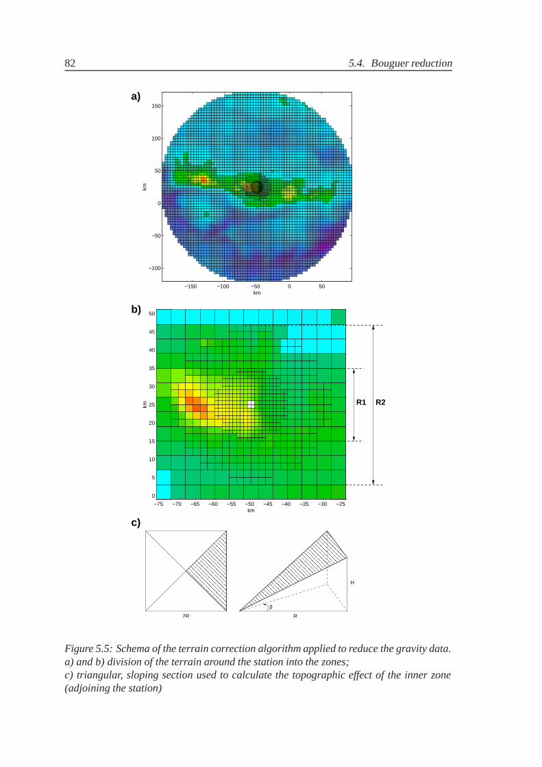
82 5.4. Bouguer reduction
�����������������������������������������������������������������������������
�����������������������������������������������������������������������������
2R ���������������������������������������������������������������������������������������������������������������������������������������������������������������������
���������������������������������������������������������������������������������������������������������������������������������������������������������������������
β
R
H
−150 −100 −50 0 50
−100
−50
0
50
100
150
km
km
−75 −70 −65 −60 −55 −50 −45 −40 −35 −30 −25
0
5
10
15
20
25
30
35
40
45
50
km
km
a)
b)
c)
R1 R2
Figure 5.5: Schema of the terrain correction algorithm applied to reduce the gravity data.a) and b) division of the terrain around the station into the zones;c) triangular, sloping section used to calculate the topographic effect of the inner zone(adjoining the station)

CHAPTER 5. Gravity field of the Hellenic subduction zone 83
Figure 5.6: Bouguer gravity field. Reduction density ρBouguer = 2.67g/cm3
84 5.5. Notes about the accuracy of gravity data
north of the island and in the southern corners of the region. The characteristic feature
of the Bouguer field is the arc-shaped zone of the relative low gravity field that extends
from the Peloponessos, through Crete and Rhodos to Anatolia. This zone is followed to
the north by a quasi arc-shaped zone of the gravity high. The anomalies south of Crete
are not so regular. High gravity anomalies are divided by two regions of significant low
gravity field. Moreover, the anomalies show very high horizontal gradients. At a distance
of less then 100 km the gravity field raises from -20 mGal to nearly +150 mGal (south of
Crete). The southernmost gravity field is characterized by high anomalies with a zone of
the relative low gravity field in the central part.
5.5 Notes about the accuracy of gravity data
It is difficult to estimate a general accuracy of the collected gravity anomalies. The fact
that the observations come from different sources causes that the accuracy extends from
less then 1 mGal (land observations on Crete) to more than 5 mGal of the satellite derived
gravity field. Figure 5.2 shows that the inaccuracy of the satellite data extends 10 mGal.
One should notice that the satellite observations have their maximal errors at the areas
covered by surface measurements. Therefore, the actual inaccuracy of this data set can be
estimated to be in a range of 5-10 mGal. However, one should be aware that local errors
in the satellite derived gravity field can be greater.
The other factor that can increase the inaccuracy of the Bouguer anomalies is the applied
terrain correction. The topography surrounding each gravity station was approximated by
prismatic bodies of 1 km minimum width. The relief of the region adjacent to a gravity
station was approximated by sloping sections which improved the accuracy. However, in
the presence of a very rough topography this approximation may be not sufficient. An
escarpment of 200 m height in a distance of 200 m from an observation point can produce
a gravity effect of about 10 mGal. Such a situation exists only in some areas of the HSZ
and possible errors have a local character and can be easily eliminated.
Figure 5.7 shows two gravity profiles crossing Crete. They present free-air and Bouguer
gravity anomalies with distinction to different sources of these data. The plots show that
the gravity field derived from the satellite altimetry is on the relative same level as the
shipborne gravity field. The significant discrepancy in the FA anomalies, which exists
between the shipborne and land observations at the WE profile is due to the steep coast of
Crete. This discrepancy is no more observed in the Bouguer anomalies.

CHAPTER 5. Gravity field of the Hellenic subduction zone 85
Figure 5.7: FA and Bouguer anomalies from different sources: red - satellite derived data,blue - shipborne data, green - land data.a) SN profile crossing central Creteb) WE profile crossing Crete

86 5.5. Notes about the accuracy of gravity data

Chapter 6
Interpretation of gravity data.
6.1 Introduction
The gravity anomalies presented in the previous chapter cover the whole investigated area.
The geophysical observations presented in the Chapter 4 gave local information about the
structure of the lithosphere of the HSZ . Seismic surveys provide usually 1D (e.g. ESP)
or 2D (e.g. WARRP profiles) data. Geological investigation of marine areas with seismic
or seismological methods is sometimes a very difficult task. GPS measurements, on the
other hand, give a very general overview about the tectonics of the southern Aegean.
Therefore, gravimetric methods can be applied to fill out the gap between these data
sources. Using the information from geology and other geophysical methods, gravimetry
is able to deliver a 3D continuous density model of the subduction zone. The cooperation
with other methods is very important because gravimetry as a method dealing with a
potential field suffers from non-uniqueness of the interpretation.
One of the first attempts to apply gravity modeling to investigate the structure of the crust
in the HSZ was done by Truffert et al. (1993). They constructed a 2D density model to
test the structure deduced from the ESP observations. Within the present project, first
gravity modelings were done by means of IGMAS. The model resulting from this early
part of the project (see Casten and Snopek, 2004) gave a general overview of the main
structural units of the subduction zone. That model, however, was constructed with the
assumption that the modeled geological layers have constant density. Moreover, modeling
with a program based on the polyhedron approach requires a clear vision of the modeled
structure. On account of the tectonic complexity of the Hellenic subduction zone and
relative few seismic constraints on densities it was very difficult to prepare one universal
starting model with IGMAS. The approach used by 3GRAINS gives more freedom in
87

88 6.2. 3GRAINS modeling
modeling and, what is more important, enables application of automatic analysis methods:
ES inversion and grid search analysis.
6.2 3GRAINS modeling
Modeling with 3GRAINS was concerned with the lithosphere and was addressed to solve
the following problems:
• thickness of the continental crust below Crete and its vicinity i.e. existence of the
mantle wedge between the Cretan crust and the subducting oceanic plate,
• Moho depth below the Cretan Sea and Cyclades,
• density variations of the crust and mantle,
• source of the very strong horizontal gradient in the gravity anomalies south of Crete.
6.2.1 Model characteristics
The model covered the area of 300×400 km with Crete in the central position (see Figure
6.1). Although the stated problems deal mainly with the upper part of the lithosphere
(≈ 50 km depth) the model must include also the deeper parts of the earth. The reason
for that is a very high curvature of the Wadati-Benioff zone (see Figure 4.3 on page 62)
and probably a significant gravity effect of the subducting African lithosphere. The slab
is observed at a depth of 150 km below the northern part of the region, so the vertical size
of the model was also set to 150 km.
The Bouguer anomalies used in the modeling were averaged on a 10× 10 km grid giving
2091 data points. The model should compromise the acceptable good resolution with its
reasonable size. The width and length of blocks constituting the model was the same as
the interval of gravity stations i.e. 10 km (see Figure 6.1, upper plot). The height of the
blocks varied with depth and reflected the complexity and relief of the modeled structural
units. The height of the blocks within the first 5 km was set to 1km which was enough to
model the sea bottom. The blocks that were used to model the crust (between 5 and 55
km) had a height of 2.5 km. Finally the blocks constituting the upper mantle had heights:
5 km (between 55 and 100 km) and 10 km at the deepest part of the model (see Figure 6.1
lower plot). Hence, the model was divided into 50 × 40 × 39 = 78000 blocks.

CHAPTER 6. Interpretation of gravity data. 89
10 x 10 km
x = 400 kmy
= 5
00 k
mz
= 1
50 k
m
1km
2.5 km
5 km
10 km
Figure 6.1: Layout of the 3GRAINS model of the HSZ (numbers next to the bracketsindicate the vertical size of blocks).

90 6.2. 3GRAINS modeling
Each block could be assigned to one of the defined layers: seawater, sediments, upper and
lower continental crust, oceanic crust, upper mantle (divided into the African and Aegean
one) and asthenosphere (see Table 6.1). Densities of the crustal layers were estimated
from the WARRP profiles applying the Nafe&Drake relation between P-wave velocities
and densities (e.g. Ludwig et al., 1971). The following assumptions were included by the
determination of mantle densities:
• the African continental mantle has a standard mantle density ( ρAM(c) = 3.35 −3.4 g/cm3, e.g. PREM by Dziewonski and Anderson, 1981),
• density of the old and “cold” African oceanic mantle is increased to ρAM(O) =
3.4 g/cm3,
• density of the “hot” Aegean mantle is decreased to ρEM = 3.25 − 3.35 g/cm3,
• and density of the asthenosphere is ρA = 3.35 g/cm3.
It is important to stress that by gravity modeling only relations between densities of the
particular layers are important. The densities of the mantle layers can differ from the real
ones but their relative values are similar to the values observed in other subduction zones
(e.g. Grow and Brown, 1975) and should enable a correct modeling of the mantle gravity
effect. Table 6.1 gives a summary of the modeled layers, observed P-wave velocities and
applied densities. The initial density means the density which was used during the model
creation. In the following, the term crust will refer only to the crystalline crust i.e. the
crust of density greater than 2.6 g/cm3. The term Moho, if not specified, will refer to the
continental Moho i.e. the LC-EM boundary.
The relief of the sea bottom was automatically imported from the available bathymetric
data and of course was not the object of the interpretation. The described model (i.e.
including all defined layers and extending to 150 km depth) will be referred as the litho-
spheric one in the following.
The reference density used in the interpretation was equal to the initial density of the
Aegean mantle: ρref = 3.3 g/cm3
6.2.2 Lithospheric model and field separation.
The presented model consisted of a great number of blocks and stations. The work
with such a model required a very powerful computer (the size of the model after equa-
tion 2.4 on page 20 was almost 300 MB). It was still possible to work with such a model

CHAPTER 6. Interpretation of gravity data. 91
LAYERP WAVE VELOCITY
[km/s]
INITIAL DENSITY
[g/cm3]
DENSITY RANGE
[g/cm3]
Seawater (SW) - 2.67(*) -
Sediments (S) 2.5-4.9 1.9-2.6 1.9-2.6
Upper crust (UC) 5.8-6.4 2.67 2.6 -2.75
Lower crust (LC) 6.5-6.9 2.85 2.75-2.95
Oceanic crust (OC) 6.9-7.1 2.95 2.95
African mantle (AM) 7.9 3.35 3.35-3.4
European mantle (EM) 7.7 3.3 3.25-3.35
Asthenosphere (A) - 3.35 3.35
Table 6.1: Modeled layers. (*)Topographic reduction density.

92 6.2. 3GRAINS modeling
AM
AM
LC
S
A
EM
OC
UCS
SW
EM
S
Figure 6.2: Layers layout
but a smaller one would have speed up the calculations. The rational solution would be a
reduction of the model size. The model should clear up the crustal structure of the HSZ.
Therefore it should deal with a depth of up to 50 km. The length and width of the mod-
eled area was several hundreds of kilometers and the gravity effect of the deeper parts of
the model could not be neglected. The standard procedure in such a case is a separation
of the gravity field by means of filtering.
The most common filtering methods applied in gravimetry is spatial filtering (by means
of polynomials) and frequency domain operations: low pass filtering or upward contin-
uation of the field. All these methods assume that the gravity effect from deeper parts
is, in general, represented by anomalies of longer wavelengths then the gravity field of
surface-near parts. The HSZ is, however, dominated by a very strong topographic and
bathymetric relief. The terrain correction was calculated with the constant Bouguer den-
sity of 2.67 g/cm3. This is the standard reduction density applied with Bouguer reduction
(see e.g. Hinze, 2003). The surface rocks e.g. marine sediments have very often different
densities than that assumed one. Therefore the topographic effect is still present in the
resulting Bouguer anomalies. This is not a problem for modeling, since the sea bottom
is known and could be modeled very accurately. This phenomenon, however, makes the
standard filtering techniques useless. The sea bottom is, with the exception of trenches,
a quite smooth surface and its gravity field would be dominated by long period anoma-
lies. Figure 6.3 shows the gravity effect of the water masses and its power spectrum. The

CHAPTER 6. Interpretation of gravity data. 93
Figure 6.3: a) Gravity effect of water masses and b) its power spectrum.

94 6.2. 3GRAINS modeling
very strong response at wave lengths of 100 km and more shows that, if the long period
anomalies of the mantle were filtered out, the remained anomalies would be disturbed.
The other way to separate the mantle gravity field from the crustal one is modeling of
the mantle effect and subtracting it from the observed field. The shape and depth of the
Wadati-Benioff zone as well as the boundary between the African and European plate is
known from the seismological and seismic observations. Basing on this information the
subducted slab was modeled (see Figure 6.4). The model did not include any information
about crustal densities (except the subducted oceanic crust). In order to obtain the gravity
effect of structures deeper than 50 km, densities of all blocks above this depth were set
to the reference density. The resulted field was subtracted from the original Bouguer
anomalies. The residual field (see Figure 6.5 ) was used in the further modeling i.e. will
be called the observed field.
On account of the presented field separation, the model depth was reduced to 50 km.
The structure of the model remained unchanged. In the obtained crustal model the upper
part of the slab was still present but its geometry remained fixed and could be used as
a constraint. Hence, the structures resulted from the crustal model could be easily re-
imported into the lithospheric model.
6.2.3 Crustal model
Constraints and inversion technique
Besides the limitation resulting from the morphology of the slab, the crustal model in-
cluded the following constraints and assumptions:
• depth of the Moho varies from 30 to 40 km below the mountain chain (the Pelo-
ponessos, Crete) and below the southern vicinity of the island,
• thickness of the crust is increased beneath western Crete,
• below the Cretan sea, thickness of the crust varies between 15-25 km,
• the crust under the Cyclades has a thickness of about 25-30 km,
• the southern boundary of the Aegean continental crust is about 100 km south of
Crete and shows a characteristic back-thrust south of western Crete ( as shown in
Figure 4.1 on page 58),
• sedimentary cover of the continental crust extends to an average depth of 5 km,

CHAPTER 6. Interpretation of gravity data. 95
Figure 6.4: a) 3D and b) contour view of top of the subducting oceanic lithosphere.

96 6.2. 3GRAINS modeling
Figure 6.5: a) Gravity field of masses below 50 km (slab effect) b) residual field.

CHAPTER 6. Interpretation of gravity data. 97
• sediments of the Mediterranean Ridge have a thickness of 15 km and are underlaid
by 7.5 km crystalline oceanic crust,
• in order to simplify modeling a boundary between UC and LC (intra-crustal bound-
ary) was set to a constant depth of 10 km (as an average value resulted from WARRP
interpretation).
A starting model was constructed using these assumptions and its gravity anomalies were
calculated. The calculated field was on a different level than the observed (i.e. residual)
anomalies. The original anomalies were measured with reference to a specific gravity
datum which take into account the whole Earth. The model, however, included only the
first 50 km of the Earth radius. On account on this phenomenon and those described on
page 19 a constant shift value must be added to the calculated field. This shift value was
equal to a mean difference between the observed and calculated field: shift = 720 mGal.
The constructed model fitted roughly into the observed gravity field. In order to get a
better match between the modeled and observed anomalies, modifications to the param-
eters of the model (Moho depth and densities of the particular layers) were applied. The
inversion was done in two steps:
• Firstly, by means of an inverse, manual modeling depth of the Moho was modeled.
In this step slight modification to the depth of the intra-crustal boundary as well as
top of UC were also applied.
• Secondly, the densities of the sediments, upper crust and the Aegean mantle were
inverted by means of automatic inversion based on ES. Densities of LC were not
inverted on account of the previous modeling of the Moho.
The available constraints did not allow to invert both parameters: density and depths of the
particular layers. Therefore, in the case of LC only its depth was modeled. The boundary
between S and UC was better constrained and only horizontal distribution of densities
within each layer was the object of inversion.
Results
Figures 6.6-6.8 present the results of the first step of the inversion (the manual inverse
modeling). The resulting crustal structure is presented in Figure 6.6 and 6.7. Figure 6.6
shows a relief of the top of the crust (upper plot) and Moho (lower plot). Division into the
oceanic and continental crust is shown by means of different color scales for the different

98 6.2. 3GRAINS modeling
Figure 6.6: 3D view of the modeled a) top and b) bottom of the continental crystallinecrust

CHAPTER 6. Interpretation of gravity data. 99
Figure 6.7: Contours of depth of the continental Moho draped on the map of depths tothe subducting slab.

100 6.2. 3GRAINS modeling
Figure 6.8: Residual anomalies resulting from the first (manual) step of inversion.
types of the crust. As already mentioned, all boundaries except the continental Moho
were generally modeled as constraints (i.e. without reference to the gravity field). The
depth of the continental Moho is the effect of the compromise between the considered
assumptions and the requirement that the modeled anomalies must fit to the observed
ones. Nevertheless, the resulting residual anomalies (Figure 6.8 ) show that both fields
coincide well with each other. The distribution of the misfits has a local character and the
standard deviation, still more than twice greater than the assumed accuracy of the gravity
data, is relative small if one consider the amplitude of the modeled anomalies (from -100
up to almost 200 mGal, see Figure 6.5).
During the automatic inversion of densities no particular constraints were applied. The
goal of that process was to obtain as good as possible match between the calculated and
observed gravity field. Densities of each layer were allowed to vary as defined in Table
6.1. Depending on a depth of a layer different smoothing factors were applied: biggest for
the mantle and smallest for the sediments. The inversion was done in the following order:
first mantle densities were optimized (Figure 6.10), than densities of the crust (Figure
6.11) and finally the densities of the sedimentary layer (Figure 6.12). The accuracy of the
final model is quite high (Figure 6.9 ). The standard deviation of 7 mGal is comparable
with the accuracy of the gravity data. The resulting densities of the particular layers are
presented in Figures 6.10-6.12.

CHAPTER 6. Interpretation of gravity data. 101
Figure 6.9: Residual anomalies resulting from the second (automatic) step of inversion.
The interpretation of the results is not straightforward. The obtained densities of the upper
crust and sediments can be explained by real changes in density or by changes in depth
of boundaries between particular layers. Gravimetry can not tell it. Moreover, in some
points the density of sediments (to which a compression, i.e. increase of density with
depth, must be considered) can not be interpreted as an average density of the column.
The shallow layers influence a gravity field much more than the deeper ones. Therefore
the inverted density of sediments should be interpreted as a kind of weighted mean density
of a column. Although these limitations, several general conclusions can be judged. Three
near-surface (of S and UC) density zones related to the tectonic division of the region can
be distinguished:
• The low density zone of the Mediterranean ridge. Low density of S is probably
due to the existence of evaporites. Because these evaporites lie near the surface,
they have more significant effect on the average density than the deeper, compacted
sediments. The lower density of UC of the Mediterranean ridge can be related to
an increased thickness of sediments (greater than assumed).
• Increased densities of UC and S of the Hellenic Arc. This is probably due to lime-
stones which were indicated by seismic experiments.
• The high density zone of the volcanic arc. Increased densities of both layers can be

102 6.2. 3GRAINS modeling
Figure 6.10: Densities of the upper mantle
caused by magmatic intrusions related to volcanism.
Besides these regional density anomalies, a local density high of the island of Gavdos is
observable. This is probably due to the crustal uplift in that place.
According to the applied smoothing factor when inverting the densities of the Aegean
mantle, the results (Figure 6.10) do not show any rapid variations. Nevertheless, the
resulting densities vary from 3.28−3.34 g/cm3. High densities of the oceanic mantle were
not inverted. Figure 6.10 shows only densities of the not-subducted slab. Lower densities
of the southern edge of the investigated region indicate African continental mantle.
The answers to questions stated in the beginning of this section can be easily read from
the vertical cross-sections of the modeled structure presented in Figures 6.13-6.15. Each

CHAPTER 6. Interpretation of gravity data. 103
Figure 6.11: Densities of the upper crust

104 6.2. 3GRAINS modeling
Figure 6.12: Densities of the sediments.

CHAPTER 6. Interpretation of gravity data. 105
EM
S
OMAM
LC
UC
SWCRETE GREECES N
OC
Figure 6.13: Lower part: Vertical S-N cross-section of the modeled structure throughwestern CreteUpper part: corresponding gravity profile: green line - the observed anomalies, red line- the calculated anomalies.
figure presents the modeled structure and gravity anomalies together with the schematic
position of the profile. Figure 6.13 and Figure 6.14 give an explanation of the strong
horizontal gradient south of Crete. In the cross-section of western Crete the continental
crust expands not so far south as in that one of central Crete. The oceanic crust, however,
has a similar structure in both cross-sections. It leads to the increased thickness of the
accreted sediments south of western Crete. Additionally, continental crust south of central
Crete is thinner than south of western Crete. Superposition of these two phenomena
causes the strong variation in the gravity field (from -90 mGal to 90 mGal at a distance of
100 km).
Depth of the crust below Crete is in agreement with expectations. It has an average value
of 30 km and is increased below western Crete. Further to the North, the crust thins out
to less than 20 km below the Cretan sea and thickens again to about 25 km below the
Cyclades (i.e. the volcanic arc).

106 6.2. 3GRAINS modeling
EM
S
OMAM
LC
UC
SWCRETES N
OC
CYCLADES
Figure 6.14: Vertical S-N cross-section of the modeled structure through central Crete.
LC
UC
W E
OC
EM
SSW
CRETE
OC
Figure 6.15: Vertical W-E cross-section of the modeled structure through Crete.

CHAPTER 6. Interpretation of gravity data. 107
6.3 Grid search analysis and alternative model of west-
ern Crete
The model presented in the previous section coincides with almost all non-gravimetric
geophysical data presented in Chapter 4. The results of the detailed seismological in-
vestigation by means of receiver functions analysis suggest, however, a different crustal
structure for western Crete (see Figure 4.4 on page 63). Endrun et al. (2004) do not ob-
serve a mantle wedge below this part of the island. In order to test whether the density
model could be varied and eventually coincide with this interpretation, a detailed analysis
of the crust in the region presented in Figure 6.16 was done.
The analysis was done by means of searching on a grid of all possible combinations of
crustal thickness and density. The programs and routines developed during the work on
ES inversion (e.g. division of a model into layered columns) could be easily adapted to
perform this kind of inversion. Searching on a grid means that model properties are ap-
proximated by a small number of parameters. The quality of the model is then calculated
for every possible combination of values of these parameters. Besides the limited num-
ber of inverted parameters, such a method of investigation requires also a not very robust
solution of the forward problem.
Figure 6.16 shows the region and parameters which were the object of the grid search
analysis. The upper plot presents a schematic view of the investigated area. Two vertical
cross-sections in the lower part of the figure give a picture of the applied technique. The
grid search analysis was done in the following way:
1. The 3GRAINS density structure was transformed into the layered column structure.
A new, local model was built only of columns inside the region of interest (Figure
6.16 - high contrast part of the vertical cross-sections). The gravity anomalies of
the outer part of the 3GRAINS model were calculated only once and then added to
the anomalies of the new model.
2. The local model included all the layers defined in the 3GRAINS model (see Table
6.1) but only three parameters were variable: density and thickness of the continen-
tal crust (LC) and density of the mantle wedge (EM) below it.
3. The grid search was done for four values of density of EM (see Figure 6.17). In
each step Moho depth was shifted from its original position and than the gravity
field of the new structure was calculated for every density of LC in the defined

108 6.4. Conclusions
range. The resulting anomalies were compared with the observed ones and the
standard deviation of misfits between these two fields was plotted as a function
of density and thickness of the crust. The whole operation was repeated for four
different values of EM.
The results of the grid search are presented in Figure 6.17. Each plot shows the results for
one value of mantle density. The white color indicates the models of minimal standard
deviation. The parameters of the original model are marked with a cross. The parameters
of one of the models which coincide with the receiver function analysis are marked with a
star. Vertical cross-sections of this alternative model are shown in Figures 6.18 and 6.19.
The grid search analysis showed one more time the non-uniqueness of gravity interpreta-
tion. The alternative model assumes an increased density of the lower crust. The average
density ρ = 2.95 g/cm3 is, however, still probable for the lower crust. Moreover, Endrun
et al. (2004) also observe increased velocities of seismic waves below western Crete. As
shown in Figure 6.17 there exist other models which would agree with the receiver func-
tion interpretations (indicated with white colors below the Moho depth of 45 km). On
account of the fact that the the originally applied density of the EM was based more on
assumptions than real constraints, these models should be also taken into consideration.
6.4 Conclusions
The interpretation of gravity data presented in this chapter included two inversion tech-
niques: trial and error and ES inversion. Most important, however, was the step of the
manual modeling. On account of the tectonic complexity of the HSZ, the density struc-
ture had to be divided into many layers and the automatic inversion could be applied only
in the limited scope. Still, the ES optimization enabled the generation of a density model
which fits almost perfectly into the observed gravity field. Certainly, one could stop the
inversion process after the manual modeling phase. Similar conclusions to these stated
on page 101 could be issued from the analysis of misfits in Figure 6.8. These misfits give
information of the qualitative nature whereas the ES optimization enabled the quantitative
interpretation.
The resulted density model included the whole knowledge gained from the other methods
presented in Chapter 4. The density model allowed to test if these local datasets coincide
with each other and with the gravity field. Such an approach seems to be the only reason-
able method of application of gravimetry in regions of complicated tectonics. Gravimetry

CHAPTER 6. Interpretation of gravity data. 109
EM {3.275; 3.3; 3.325; 3.35}
EM {3.275; 3.3; 3.325; 3.35}
W
S N
E
LC [2.75 3.0]
LC [2.75 3.0]
Figure 6.16: Region and parameters of the grid search analysis

110 6.4. Conclusions
Figure 6.17: Results of the grid search for densities below western Crete. Symbols indi-cate the parameters of the original model ( +) and the alternative model (�).

CHAPTER 6. Interpretation of gravity data. 111
AM
GREECE N
OC
OM
LC
SW CRETE
S
2.95
EM
S
2.852.85
UC
Figure 6.18: Vertical S-M cross-section of the alternative model of western Crete.
E
2.95
UCS
SW
LC
EM
2.852.85
CRETE
OC OC
W
Figure 6.19: Vertical W-E cross-section of the alternative model of western Crete.

112 6.4. Conclusions
can test and eventually exclude hypotheses from other fields, and this goal was achieved
with the presented model.
On account of the fact that the model is built of rectangular blocks, one can divide it into
smaller models and perform a detailed analysis of selected sub-regions. The presented
grid search analysis is a very effective way of exploring the parameters space in small
regions. Such an analysis requires, however, a regional model to which the local variations
of parameters can be compared. Hence, the lithospheric model can be used as a basis for
further investigation.
The presented model should be updated as soon as new constraining data (e.g. from
seismic or seismology) or gravity data are available. Some doubts about this model will
exist as long as certain regions are not covered with accurate gravity data. As shown in
Figure 5.1 on page 74, great parts of the model are covered with the altimetry derived
data. Replacement of these data with ship- or airborne measurements will improve and
verify the density model of the Hellenic subduction zone.

Chapter 7
Resume of the thesis
7.1 Review
This thesis discussed the following steps of processing and interpretation of gravity data:
• data acquisition and processing,
• parameterization and solution of the forward problem,
• inversion.
Some computations were done by means of the available functions provided with GMT
or Matlab (e.g. data interpolation or field separation). The use of Matlab was sometimes
very sophisticated, for example in the form of the terrain correction program. However,
the most important operations: gravity modeling and inversion, were done with the new
developed C++ programs. Programming and testing of the new software was a very time
consuming task. However, the effort put in this work was repaid. 3GRAINS, for example,
was not only used in the interpretation of the HSZ, but is still used by the gravimetry
working group of the institute (see e.g. Staackmann, 2004). The algorithms and functions
of ES inversion were successfully applied to invert the gravity anomalies of a buried
valley.
From the scientific point of view, the problems regarding the gravity inverse problem had
the central position in the thesis. The example of a simple three-parameter model of a
horizontal cylinder showed that there is no unique solution of the gravimetric problem.
The manual inverse modeling will remain for a long time the most important method in
113

114 7.2. Final conclusions
gravity interpretation. In some simple cases, however, the automatic inversion can sig-
nificantly speed up the interpretation. The applied rectangular blocks method enabled to
combine manual and automatic inversion methods. In the interpretation of the anomalies
of a buried valley, the the model consisted of two layers of a relative constant density
contrast. In this case, the manual modeling was limited to the preparation of the starting
model, particularly to the modeling of the edge cross-sections of the model. The auto-
matic inversion enabled a fast optimization of the columns depths inside the model.
A quite different interpretation procedure had to be applied during the inversion of gravity
data from the Hellenic subduction zone. The most important part of this interpretation was
the introduction of constraints into the density model. The automatic inversion could be
applied only in a limited scope to optimize the densities of the layers.
The new modeling software - 3GRAINS was very helpful in both cases. However, during
the work on data from HSZ the experience gained from the IGMAS modeling was very
useful. The new possibilities of the rectangular prisms method enabled faster and easier
testing of various density models.
7.2 Final conclusions
The geophysical interpretation of gravity data is a complicated and often time intensive
task. Although relative simple solution of a forward problem, the gravity inversion re-
quires a lot of experience from an interpreter. For a long time, manual and automatic
inversions were performed separately. Generally it was due to the fact that the most com-
mon parameterization used in the automatic inversion was the division of the model into a
set of small rectangular blocks while the modeling software like IGMAS applied the poly-
hedron approach. Moreover, limitations of computer power and memory suppressed the
application of rectangular blocks methods in modeling of high resolution density struc-
tures. Nowadays computers, however, enable to unify these two inversion methods. This
allows to overcome some limitations of each method:
• The severe drawback of every automatic inversion method is the introduction of
constraints. The simplest and most effective constraining method is a good prepared
(by means of the manual modeling) starting model.
• A machine is not a god. The model resulting from the automatic inversion is only
one of the possible solutions. Instant visualization of the resulting structures enables
fast estimation of the model quality and application of eventual corrections.

CHAPTER 7. Resume of the thesis 115
• The manual modeling may be a very complex task, particularly in 3D cases. The
modeling of the 3D structures is usually done by means of software that enables
operations on 2D cross-sections. Working with the one cross-section (and its gravity
profile) one must consider that the modeled masses affect also the gravity field of
the other profiles. In such cases the automatic inversion can significantly reduce the
interpretation time.
The proposed method of automatic inversion of gravity data is an universal tool. The al-
gorithm based on Evolution Strategies does not require any particular mathematical char-
acteristics of the objective function ( e.g. it does not need to be linear or differentiable).
On account of the non-uniqueness of a gravity problem, the random nature of such an
algorithm can be seen as a benefit. The randomness of the calculations may cause that
some runs do not reach a convergence but on the other hand it enables exploration of a
wide range of possible solutions.

116 7.2. Final conclusions

Appendix A
3GRAINS
A.1 Kernel compressing technique.
The compressing of the kernel array is done in two steps. In the first one, the array of real
values is recoded into the array of integer numbers. In the second one, the recoded array
is compressed with the RLE (Run Length Encoding) algorithm.
The recoding is done in the following way. For each of N stations, a real number column
vector Gi(1, ..., M) is calculated. Gi is analyzed and L different components are saved
into the array V . Two numbers are assumed to be the same if the difference between them
is smaller then some given significance threshold; elements less than the calculated or
assumed threshold value are set to zero. Gi becomes now an integer number vector Ki
with elements being positions of values Gi in the array V . For example, assume:
Gi = (3.2, 2.2, 1.0001, 1.0002, 0.000014, 0.0000026, 0.0000043,
0.99999, 0.01, 0.01001, 0.009996, 2.3, ..., GiM)
and
Gi < 0.0001 => Gi = 0
abs(Gi − Gj) < 0.0001 => Gi = Gj
then (A.1)
Ki = (1, 2, 3, 3, 0, 0, 0, 3, 4, 4, 4, 5, ..., KiM)
and
V = (0, 3.2, 2.2, 1.0, 0.01, 2.3, ..., VN)
Notice that the array V is indexed from zero !
117

118 A.2. The main windows and functions of the program
As an integer number, every component of Ki needs 2 bytes of memory. L normally does
not exceed 20 000. To win additional memory space, Ki is then compressed with the RLE
compressing algorithm.
RLE works by reducing the physical size of repeating numbers called “run”. It finds
sequences of the same elements and saves it as a pair: {run, run count}. In our example,
the compressed array Ki has the form:
Ci = ({1, 1}{2, 1}{3, 2}{0, 3}{3, 1}{4, 3}{5, 1}...) (A.2)
The run count is encoded as one byte number so each pair has the size of three bytes.
The numerical experiments show that, for example, the initial matrix G of 1.6 GB, can be
compressed to about 200 MB, which is a reasonable quantity. The compression method
presented here contains a risk that the compressed array is greater than the initial one. The
nature of the kernel matrix G allows us to expect that it is not the problem in this situation.
In the worst case the compressed kernel has the same size as the uncompressed one and
the compressing ratio increases with the size of G. The use of this compression method
allows also reducing time of computation of the model anomaly: zero components are
skipped and no needless multiplications by zero are carried out.
The first part of the presented compressing technique influences the accuracy of the pro-
gram. Replacing the real values of the kernel G with the smaller number of values V
(Equation A.1) causes very small changes in the resulting gravity field. The RLE algo-
rithm is a non-losing method so it does not produce any effects on anomalies.
A.2 The main windows and functions of the program
A.2.1 Main window
The main window of 3GRAINS (Figure A.1) contains the classical elements used in grav-
ity modeling. The modeled structure (structure plot) is accessible through two perpendic-
ular vertical cross-sections or a horizontal one. The grid showing a structure of used
prisms is visible but it can be disabled. If a vertical cross-section is selected, the gravity
anomalies of the related profile are displayed above it. The anomaly plot contains two
lines showing the measured (green, solid line) and calculated gravity field (red, dashed
line). Above the plot, on its right side the information about the actual profile is dis-
played. That is: the plane of the profile (xz, yz or xy) and its coordinates. If the actual

CHAPTER A. 3GRAINS 119
Figure A.1: Main window of 3GRAINS.
plane is xy (horizontal cross-section) the anomaly plot is hidden automatically. It can be
also hidden manually to enable more space for the modeling.
On the right side of the main window three objects are accessible: selector of layers
(combo box), reference density button and density color scale. The layers combo box
is used to select one of the predefined layers. The density color scale refers always to
the actual layer and uses the information contained in the Layers layout. The reference
density button is used to set an actual density to a reference density.
Once the actual density is selected, it can be used to change the parameters of blocks
selected on the structure plot. The selection can be done by means of one of three shape
tools (left part of the task bar). The shapes are: rectangle, ellipse and polygon. If the
rectangle shape tool is selected, the single blocks or group of blocks forming a rectangle
are marked. If the ellipse shape tool is selected, the blocks inside an ellipse are marked.
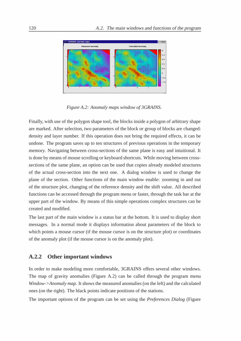
120 A.2. The main windows and functions of the program
Figure A.2: Anomaly maps window of 3GRAINS.
Finally, with use of the polygon shape tool, the blocks inside a polygon of arbitrary shape
are marked. After selection, two parameters of the block or group of blocks are changed:
density and layer number. If this operation does not bring the required effects, it can be
undone. The program saves up to ten structures of previous operations in the temporary
memory. Navigating between cross-sections of the same plane is easy and intuitional. It
is done by means of mouse scrolling or keyboard shortcuts. While moving between cross-
sections of the same plane, an option can be used that copies already modeled structures
of the actual cross-section into the next one. A dialog window is used to change the
plane of the section. Other functions of the main window enable: zooming in and out
of the structure plot, changing of the reference density and the shift value. All described
functions can be accessed through the program menu or faster, through the task bar at the
upper part of the window. By means of this simple operations complex structures can be
created and modified.
The last part of the main window is a status bar at the bottom. It is used to display short
messages. In a normal mode it displays information about parameters of the block to
which points a mouse cursor (if the mouse cursor is on the structure plot) or coordinates
of the anomaly plot (if the mouse cursor is on the anomaly plot).
A.2.2 Other important windows
In order to make modeling more comfortable, 3GRAINS offers several other windows.
The map of gravity anomalies (Figure A.2) can be called through the program menu
Window->Anomaly map. It shows the measured anomalies (on the left) and the calculated
ones (on the right). The black points indicate positions of the stations.
The important options of the program can be set using the Preferences Dialog (Figure

CHAPTER A. 3GRAINS 121
Figure A.3: Preferences dialog of 3GRAINS
A.3). It enables modification of the following parameters :
Instant anomaly calculation If set to yes the anomaly is calculated after every modifica-
tion of the modeled structure. Otherwise the anomaly is calculated when the menu
Model->Calculate anomaly is called or the anomaly button is clicked.
Profile steps Define the value of which the cross-section coordinate will be changed
when the user moves between cross-sections of the same plane.
Anomaly y-axis Defines limits of the anomaly axis. Enables automatic or manual modes.
Calculate separate layers effect If set to yes only anomaly of blocks belonging to the
selected layer is calculated. Otherwise the effect of all blocks is calculated.
Model parameters Enables modification of reference density and shift value. A button
for automatic calculation of shift value is provided.
A.2.3 Input-output functions
Operations that enable saving the results and exchanging data between the main program
and other programs are a very important part of every geophysical application. 3GRAINS
provides several exporting options that allow saving (to ASCII file) of:

122 A.2. The main windows and functions of the program
• calculated anomaly of the whole structure or the particular layer,
• the whole numerical model of the modeled structure,
• depths of boundaries between the defined layers,
• densities of the selected layer,
• densities of a horizontal slice of the selected depth.
The main goal of these functions is to provide data for external graphical programs.
3GRAINS does not offer any options for viewing 3D structures. This task should be
accomplished by means of external programs e.g. GMT (Generic Mapping Tools). Such
programs offer advanced techniques to produce 2D or 3D plots of various data sets. The
exporting functions are available not only from 3GRAINS main window, but exist also as
standalone shell1 programs. The syntax of these programs is similar to GMT commands.
Hence, visualization of models prepared with 3GRAINS can be automatized and done
outside the graphical module of the program.
The only graphical export option is the possibility of saving the image of the actual se-
lected cross-section (with its anomaly plot) to a graphic file.
The exported structures can be modified outside 3GRAINS (i.e. by means of an auto-
matic inversion program) and re-imported to the program. The user can also import the
anomalies from ASCII files.
1Shell: in Unix based systems (e.g. Linux), the command interpreter used to pass commands to anoperating system; so called because it is the part of the operating system that interfaces with the outsideworld

Appendix B
ES inversion
B.1 Parallel computing
The ES based inversion is a very time intensive task. During the inversion of HSZ data
each model consisted of almost 2000 columns and the population of λ = 16, µ = 96 was
used. In every generation each model need to be evaluated (i.e. its gravity response is
calculated), mutated and recombinated. Processing of only one model lasted about one
minute, and the time needed for the whole population would be almost two hours. There-
fore the calculations were processed on a parallel computer which enabled calculations of
the models simultaneously.
The GMG institute of Ruhr University of Bochum uses a LAN-based cluster built of
18 2CPU units (see Röcher, 2002). PC clusters are a cheap alternative to conventional
supercomputers. A PC cluster is made by linking inexpensive PCs and writing software
(usually under Linux) that allows these ordinary computers to act as one supercomputer.
It usually consists of one control PC (master) and number of nodes (or “slaves”) (see e.g.
Sterling et al., 1999; Hoffman and Hargrove, 1999).
The strategy of parallel computing is to divide a problem into small tasks that can be
maintained simultaneously. Not every algorithm can be rewritten in a parallel form. Most
methods of inversion or parameter optimization e.g. gradient methods are inherently se-
quential due to their iterative nature or may be only parallelized by vectorizing some of
their internal operations.
The evolutionary algorithms are very suitable for parallel implementation. Operations
like evaluation, mutation and partially recombination are independent from each other
and can be processed at the same time. The efficiency of parallel processing on a PC clus-
123

124 B.1. Parallel computing
ter depends on the nature of the problem. An important consideration is how often the
nodes must communicate to coordinate their work and to share intermediate results. Some
problems need to be divided into a large number of sub-tasks with low computational re-
quirements but with high demands on communication between nodes. These fine-grained
problems are not very well suited for parallel processing on PC clusters. The other class of
problems are coarse-grained ones. They consists of a few compute-intensive tasks with a
little communication demand. Depending on a problem and a implementation the EA can
fall into one of these groups. This theme is discussed by Hoffmeister and Bäck (1991).
The implementation which was applied to invert the anomalies of the buried valley and
HSZ looks like it is shown in Figure B.1. A single control process (master) generates the
population and selects the parents of the next generations. The selected parents are sent
to other processors (slaves) in pairs where all robust calculations are processed simulta-
neously. The evaluated offspring is sent back to the master where the selection of the next
generation is done. Such an approach requires communication between the master and
slaves two times per generation. Because mutation, recombination and evaluation takes
more than 90% of time needed to process one generation, this implementation enables to
reduce significantly computation time.
If every processor maintained a pair of individuals then the maximum size of population
would be 18 × 2 × 2 = 72 (the PC cluster consists of 18 computers). Greater population
could be used if slaves processed 4,6.. individuals (the even number is required in order
to enable recombination). In the presented example 16 processors were used and every
one maintained 2 pairs i.e. 4 individuals.

CHAPTER B. ES inversion 125
Primergy
Primergy
Primergy
Primergy
Primergy
Primergy
Evaluation
Initialization
Parent Selection
Recombination
Mutation
Evaluation
Survivor Selection
Check end conditions END
MASTER SLAVES
Figure B.1: Parallel implementation of ES.

126 B.2. Random numbers generator
B.2 Random numbers generator
A generator of random numbers is an essential part of every algorithm of Evolutionary
Computation. In this thesis the Mersenne Twister random number generator developed by
Matsumoto and Nishimura (1998) was used. The C++ implementation of this algorithm
was developed by Richard J. Wagner Copyright (C) 2002.
The Mersenne Twister algorithm generates uniformly distributed random numbers in the
range [0, 1]. To proceed the mutation, the normal distributed numbers were needed. These
were generated using the following pseudo code:
rand(); // Mersenne Twister generator
normal() // Gaussian generator
{
x = 0;
for(int i=0;i<12;i++)
x = x + rand();
return x-6;
}
The function normal() returns normally distributed random numbers with the mean µ = 0
and the standard deviation σ = 1. In order to generate numbers with another mean and
standard deviation the following function was used:
normal(µ, σ)
{
return µ + σ ∗ normal()
}

Bibliography
Advanced National Seismic System, ANSS. http://quake.geo.berkeley.edu/anss.
Angelier, J., Lybéris, N., Pichon, X. L., Barrier, E., Huchon, P., 1982. The tectonic de-
veleopment of the Hellenic arc and the Sea of Crete: a synthesis. Tectonophysics 86,
159–196.
Bohnhoff, M., Makris, J., Papanikolaou, D., Stavrakakis, G., 2001. Crustal investigation
of the Hellenic subduction zone using wide aperture seismic data. Tectonophys. 343 (3-
4), 239–262.
Brandt, S., 1970. Statistical and Computational Methods in Data Analysis. North-Holland
Publishing Company, Amsterdam.
Brönner, M., 2003. Untersuchung des Krustenaufbaus entlang des Mediterranen Rückens
abgeleitet aus geophysikalischen Messungen. In: Berichte aus dem Zentrum für Meeres
und Klimaforschung, Reihe C: Geophysik Nr. 21. Universität Hamburg, p. 170.
Carmichael, R., Henry, G., 1977. Gravity exploration for groundwater and bedrock to-
pography in glaciated areas. Geophysics 42 (4), 850–859.
Casten, U., Snopek, K., 2004. Gravity modelling of the Hellenic subduction zone - a
regional study. Submitted to Tectonophysics.
Chakravarthi, V., Raghuram, H. M., Singh, S., 2002. 3-D forward gravity modeling of
basement interfaces above which the density contrast varies continously with depth.
Geophysics 28, 53–57.
Chapin, D., 1998. Gravity instruments: Past, present, future. The Leading Edge 17, 100–
112.
Chaumillon, E., Mascle, J., 1997. From foreland to forearc domain: New multichannel
seismic reflection surveys of the Mediterranean ridge accrectionary complex (Eastern
Mediterranean). Marine Geology 138, 237–259.
127

128 BIBLIOGRAPHY
Cordell, L., Henderson, R., 1968. Iterative three-dimensional solution of gravity anomaly
data using a digital computer. Geophysics 33, 596–601.
de Voogd, B., Truffel, C., Chamot-Rooke, N., Huchon, P., Lallemant, S., Pichon, X. L.,
1992. Two-ship deep seismic soundings in the basin of the Eastern Mediterranean Sea
(Pasiphae Cruise). Geophys. J. Int. 109, 536–552.
Dziewonski, A., Anderson, D., 1981. Preliminary Reference Earth Model. Phys. Earth
planet. Inter. 25, 297.
Endrun, B., Meier, T., Bischoff, M., Harjes, H.-P., 2004. Lithospheric structure in the area
of Crete constrained by receiver functions and dispersion analysis of Rayleigh phase
velocities. Geophys. J. Int. 158, 592–608.
Fruehn, J., Reston, T., von Huene, R., Bialas, J., 2002. Structure of the Mediterranean
Ridge accretionary complex from seismic velocity information. Marine Geology 186,
43–58.
Generic Mapping Tools, GMT. http://gmt.soest.havaii.edu.
Götze, H.-J., Lahmeyer, B., 1988. Application of three-dimensional interactive modelling
in gravity and magnetics. Geophysics 53, 1096–1108.
Granser, H., 1987. Three-dimensional interpretation of gravity data from sedimentary
basins using an expotential density-depth function. Geophysical Prospecting 35 (9),
1030–1041.
Grow, J. A., Brown, C., 1975. Evidence for high-density crust and mantle beneath th Chile
trench to to descnending lithopshere. J. Geophys. Res. 80, 1449–1458.
Hinze, W. J., 2003. Bouguer reduction density, why 2.67. Geophysics 68 (5), 1559–1560.
Hoffman, F. M., Hargrove, W., 1999. Cluster Computing: Linux Taken to the Extreme.
Linux Magazine 1 (1), 56–59.
Hoffmeister, F., Bäck, T., 1991. Genetic algorithms and evolution strategies: similari-
ties and differences. In: Parallel Problem Solving from Nature - Proceedings of 1st
Workshop, PPSN 1. Vol. 496 of Lecture Notes in Computer Science. Springer-Verlag,
Berlin.
Holland, J., 1975. Adaptation in natural and artificial systems. University of Michigan
Press, Ann Arbor, MI.

BIBLIOGRAPHY 129
Holstein, H., Schürholz, P., Starr, A. J., Chakraborty, M., 1999. Comparison of gravimet-
ric formulas for uniform polyhedra. Geophysics 64 (5), 1438–1446.
Huchon, P., Lyberis, N., Angelier, J., Pichon, X. L., Renard, V., 1982. Tectonics of the
Hellenic Trench: A synthesis of Sea-Beam and submersible observations. Tectono-
physics 86, 69–112.
Huguen, C., Mascle, J., Chaumilion, E., Woodside, J. M., Benkhelil, J., Kopf, A.,
Volkonkaia, A., 2001. Deformational styles of the eastern Mediterranean Ridge and
surroundings from combined swath mapping and seismic reflection profiling. Tectono-
physics 343, 21–47.
Ilinski, D., Makris, J., Casten, U., 2001. A density model of the Hellenic collision zone
at the island of Crete. . European Geophysical Society, 26th General Assembly, Nice,
France, 25-30 March 2001. Geophysical Research Abstracts 3 (CD).
Interactive Gravity and Magnetic Application System, IGMAS. http://userpage.fu-
berlin.de/˜sschmidt/Sabine_IGMAS.html.
Jain, A., 1986. Fundamentals of Digital Image Processing. Prentice-Hall.
Koblinsky, C., Beckley, B., Ray, R., Wang, Y.-M., Brenner, A., Apr. 1999. NASA Ocean
Altimeter Pathfinder Project. In: Report 1: Data Processing Handbook. NASA/TM-
1998-208605.
Lallemant, S., Truffert, C., Jolivet, C., Henry, P., Chamot-Rooke, N., de Voogd, B., 1994.
Spatial transition from compression to extension in the Western Mediterranean Ridge
accretionary complex. Tectonophysics 234, 33–52.
Lambeck, K., 1995. Late Pleistocene and Holocene sea-level change in Greece and south-
western Turkey: a separation of eustatic, isostatic and tectonic contributions. Geophys.
J. Int. 122, 1022–1044.
Ludwig, W. J., Nafe, J., Drake, C., 1971. Seismic refraction. In: A.E. Maxwell(ed) The
Sea. Vol. 4. John Wiley & Sons, New York, pp. 53–84.
Matsumoto, M., Nishimura, T., Jan. 1998. "Mersenne Twister: A 623-Dimensionally
Equidistributed Uniform Pseudo-Random Number Generator. ACM Transactions on
Modeling and Computer Simulation 8 (1), 3–30.

130 BIBLIOGRAPHY
McClusky, A., Balassanian, S., Barka, A., Demir, C., Ergintav, S., Georgiev, I., Gurkan,
O., Hamburger, M., Hurst, K., Kahle, H., Kastens, K., Kekelidze, G., King, R., Kotzev,
V., Lenk, O., Mahmoud, S., Mishin, A., Nadariya, M., Ouzounis, A., Paradissis, D., Pe-
ter, Y., Prilepin, M., Reilinger, R., Sanli, I., Seeger, H., Tealeb, A., Toksoz, M. N., Veis,
G., 2000. Global Positioning System constraints on plate kinematics and dynamics in
the eastern Mediterranean and Caucasus. J. Geophys. Res. 105 (B3), 5695–5719.
Meier, T., Dietrich, K., Stöckhert, B., Harjes, H.-P., 2004a. One-dimensional models
of shear wave velocity for the estern Mediterranean obtained from the inversion of
Rayleigh wave phase velocities and tectonic implications. Geophys. J. Int. 156, 45–58.
Meier, T., Rische, M., Endrun, B., Vafidis, A., Harjes, H.-P., 2004b. Seismicity of the Hel-
lenic subduction zone in the area of western and central Crete observed by temporary
local seismic networks. Tectonophysics 383, 149–169.
Meulenkamp, J., van der Zwaan, G., van Wamel, W., 1994. On Late Miocene to Recent
vertical motions in the Cretan segement of the Hellenic arc. Tectonophysics 234, 53–
72.
Nagy, D., 1966. The gravitational attraction of a right rectangular prism. Geophysics 31,
362–371.
Papazachos, B., Comninakis, P., 1971. Geophysical and Tectonic Features of the Aegean
Arc. J. Geophys. Res. 76 (35), 8517–8533.
Papazachos, B., Karakostas, V., Papazachos, C., Scordilis, E., 2000. The geometry of the
Wadati-Benioff zone and litospheric kinematics in the Hellenic arc. Tectonophysics
319, 275–300.
Papazachos, C., Nolet, G., 1997. P and S deep velocity of the Hellenic area obtained by
robust nonlinear inversion of travel times. J. Geophys. Res. 102, 8349–8367.
Papazachos, C. B., Hatzidimitriou, P. M., Panagiotopoulos, D. G., Tsokas, G. N., 1995.
Tomography of the crust and upper mantle in southeast Europe. J. Geophys. Res. 100,
12405–12422.
Pichon, X. L., Chamot-Rooke, N., Lallemant, S., Noomen, R., Veis, G., 1995. Geodetic
determination of the kinematics of central Greece with respect to Europe: Implications
for eastern Mediterranean tectonics. J. Geophys. Res. 100, 12675–12690.

BIBLIOGRAPHY 131
Rechenberg, I., 1973. Evolutionsstrategie: optimierung technischer systeme nach prinzip-
ien der biologischen evolution. Frommann-Holzboog, Stuttgart.
Röcher, D.-J., 2002. A parallel algorithm for three-dimensional gravity modellilng and
inversion. Diploma thesis, Ruhr Univercity Bochum.
Sandwell, D., Smith, W., 1997. Marine Gravity from Geosat and ERS 1 Satellite Altime-
try. J. Geophys. Res. 102 (B5), 10039–10054.
Schwefel, H. P., 1981. Numerical Optimisation of Computer Models. Wiley, Chichester.
Silva, J. B. C., Medeiros, W., Barbosa, V. C. F., 2001. Potential field inversion: Choosing
the appropiate technique to solve a geologic problem. Geophysics 66 (2), 511–520.
Smith, W. H. F., Sandwell, D. T., 26 September 1997. Global Seafloor Topography from
Satellite Altimetry and Ship Depth Soundings. Science 277, 1956–1962.
Staackmann, M., 2004. 3D gravimetrische Modellierung der Oberkruste von Kreta.
Diploma thesis, Ruhr University Bochum.
Sterling, T., Salmon, J., Becker, D. J., Savarese, D. F. (Eds.), 1999. How to Build a
Beowulf: A Guide to the Implementation and Application of PC Clusters. MIT Press.
Talwani, M., Ewing, M., 1960. Rapid computation of gravitational attraction of three-
dimensional bodies of arbitrary shape. Geophysics 25, 203–225.
Talwani, M., Worzel, J., Landisman, M., 1959. Rapid gravity computations for two-
dimensional bodies with application to the Mendocino submarine fracture zone. J. Geo-
phys. Res. 64, 49–59.
Tarantola, A., 1987. Inverse Problem Theory: Methods for Data Fitting and Model Pa-
rameter Estimation. Elsevier, Amsterdam.
The Global Land One-km Base Elevation, GLOBE. http://www.ngdc.noaa.gov.
Trolltech, Qt. http://www.trolltech.com.
Truffert, C., Chamot-Rooke, N., Lallemant, S., Voogd, B. D., Huchon, P., Pichon, X. L.,
1993. The crust of the Western Mediterranean Ridge from seismic data and gravity
modelling. Geophys. J. Int. 114 (2), 360–372.

132 BIBLIOGRAPHY
Westbrook, G., Reston, T., 2002. The accretionary complex of the Mediterranean Ridge:
tectonics, fluid flow and the information of brine lakes - an introduction to the special
issue of Marine Geology. Marine Geology 186, 1–8.
Williams, G., 1997. The Pony Fish’s Glow and Other Clues to Plan and Purpose in Nature.
Orion Publishing Group Ltd., UK.
Won, I. J., Bevis, M. G., 1987. Computing the gravitational and magnetic anomalies due
to a polygon: Algorithms and Fortran subroutines. Geophysics 52, 232–238.