investment return assumptions for non-fixed income...
TRANSCRIPT

Members should be familiar with educational notes. Educational notes describe but do not recommend practice in illustrative situations. They do not constitute Standards of Practice and are, therefore, not binding. They are, however, intended to illustrate the application (but not necessarily
the only application) of the Standards of Practice, so there should be no conflict between them. They are intended to assist actuaries in applying Standards of Practice in respect of specific matters.
Responsibility for the manner of application of Standards of Practice in specific circumstances remains that of the members in the life insurance practice area.
Educational Note
Investment Return Assumptions for Non-Fixed Income Assets
for Life Insurers
Committee on Life Insurance Financial Reporting
March 2011
Document 211027 Ce document est disponible en français
© 2011 Canadian Institute of Actuaries
Memorandum
To: All Life Insurance Practitioners
From: Tyrone G. Faulds, Chair Practice Council
Edward Gibson, Chair Committee on Life Insurance Financial Reporting
Date: March 1, 2011
Subject: Educational Note – Investment Return Assumptions for Non-Fixed Income Assets for Life Insurers
The Committee on Life Insurance Financial Reporting (CLIFR) had previously issued guidance in its November 2009 educational note on Guidance for the 2009 Valuation of Policy Liabilities of Life Insurers (and earlier years) relating to the application of paragraphs 2340.11 and 2340.13 of the Standards of Practice on the use of benchmarks in setting expected returns, and the establishment of an additional margin through the assumption of a percentage reduction in the market value for non-fixed income assets. This educational note presents considerations and examples of the application of the Standards of Practice to the valuation of insurance liabilities that are matched in, part or whole, by non-fixed income assets.
In accordance with the Canadian Institute of Actuaries’ (CIA) Policy on Due Process for the Approval of Guidance Material Other than Standards of Practice, this educational note has been prepared by the Committee on Life Insurance Financial Reporting and has received final approval for distribution by the Practice Council on November 25, 2010.
As outlined in subsection 1220 of the Standards of Practice, “The actuary should be familiar with relevant Educational Notes and other designated educational material.” That subsection explains further that a “practice which the Educational Notes describe for a situation is not necessarily the only accepted practice for that situation and is not necessarily accepted actuarial practice for a different situation.” As well, “Educational Notes are intended to illustrate the application (but not necessarily the only application) of the Standards, so there should be no conflict between them.”
We would like to thank the members of CLIFR subcommittee who were primarily responsible for the development of this educational note: David Campbell, Edward Gibson, Martin Labelle, Leonard Pressey and Jim Snell.
If you have any questions or comments regarding this educational note, please contact Edward Gibson at his CIA Online Directory address, [email protected].
TGF, EG

Educational Note March 2011
3
TABLE OF CONTENTS
1. INTRODUCTION..................................................................................................................... 5
1.1 Purpose and Scope ........................................................................................................... 5
1.2 General Considerations .................................................................................................... 6
1.3 Overview of Approach ..................................................................................................... 8
1.4 Other Non-Fixed Income Assets ...................................................................................... 9
2. SELECTION OF BENCHMARKS ........................................................................................ 10
2.1 Class and Characteristics ................................................................................................ 10
2.2 Historical Period ............................................................................................................. 10
2.3 Benchmarks Meeting Criteria ........................................................................................ 11
3. BEST ESTIMATE INVESTMENT RETURNS .................................................................... 12
3.1 Geometric vs. Arithmetic Mean ..................................................................................... 12
3.2 Currency Exchange Rates .............................................................................................. 12
3.3 Investment Expenses ...................................................................................................... 12
3.4 Multiple Non-Fixed Income Assets ............................................................................... 12
3.5 Allowance for Recent Market Experience ..................................................................... 13
3.6 Frequency of Updates ..................................................................................................... 13
4. COMMON SHARE DIVIDEND AND REAL ESTATE RENTAL INCOME ..................... 14
4.1 Dividend Yields .............................................................................................................. 14
4.2 Impact of Market Shift on Projected Dividends and Rental Income ............................. 17
4.3 Taxation of Dividends and Rental Income ..................................................................... 18
4.4 Margins for Adverse Deviations .................................................................................... 19
5. MARGINS FOR ADVERSE DEVIATIONS FOR COMMON SHARE AND REAL ESTATE CAPITAL GAINS .......................................................................................... 19
5.1 Relative Volatility .......................................................................................................... 19
5.2 Diversified North American Portfolio ............................................................................ 19
5.3 Selection of Market Shift Assumption ........................................................................... 21
5.4 Net Risk Premiums ......................................................................................................... 22
5.5 Higher Relative Volatilities ............................................................................................ 23
5.6 Real Estate Market Shifts ............................................................................................... 25
5.7 Timing of Change in Market Shift ................................................................................. 25
5.8 Increase or Decrease in Market Shift ............................................................................. 25

Educational Note March 2011
4
5.9 Other Considerations ...................................................................................................... 26
APPENDICES A: DESCRIPTIONS OF BENCHMARK INDICES – EQUITIES ............................................... 27
1. Canadian Equities – S&P/TSX Composite .................................................................... 27
2. U.S. Equities – S&P 500 ................................................................................................ 28
3. U.S. Equities – NASDAQ Composite ............................................................................ 28
4. Foreign Equities – UK .................................................................................................... 29
5. Foreign Equities – MSCI EAFE ..................................................................................... 30
6. Foreign Equities – Japanese ........................................................................................... 31
7. Foreign Equities – Hong Kong ....................................................................................... 31
B: DESCRIPTIONS OF BENCHMARK INDICES – REAL ESTATE ....................................... 33
1. Canadian Real Estate – ICREIM/IPD Canada ............................................................... 33
2. U.S. Real Estate – NCREIF Property ............................................................................. 33
C: ILLUSTRATION OF PROJECTED EQUITY RETURNS ...................................................... 35
D: STOCHASTIC INVESTMENT MODEL PARAMETERS ..................................................... 38
1. S&P/TSX Composite Index ........................................................................................... 38
2. Hang Seng Index ............................................................................................................ 38
E: EXAMPLE OF EQUITY RETURNS FOR EMERGING MARKETS .................................... 40
Educational Note March 2011
5
1. INTRODUCTION 1.1 Purpose and Scope This educational note describes considerations for selecting best estimate investment return assumptions and margins for adverse deviations (MfADs) for non-fixed income assets when used in deterministic scenarios for the valuation of policy liabilities of life insurers. Paragraphs 2340.11 through 2340.14 of the Standards of Practice read,
.11 The actuary’s best estimate of investment return on a non-fixed income asset would not be more favourable than a benchmark based on historical performance of assets of its class and characteristics.
.12 The low and high margins for adverse deviations in the assumptions of common share dividends and real estate rental income would be respectively 5% and 20%.
.13 The margin for adverse deviations in the assumption of common share and real estate capital gains is 20% of the best estimate plus an assumption that those assets change in value at the time when the change is most adverse. That time would be determined by testing, but usually would be the time when their book value is largest. The assumed change as a percentage of market value
of a diversified portfolio of North American common shares would be 30%, and of any other portfolio would be in the range of 25% to 40% depending on the relative volatility of the two portfolios.
.14 Whether the assumed change is a gain or loss would depend on its effect on benefits to policy owners. A capital loss may reduce insurance contract liabilities as a result of that effect.
Non-fixed income assets include
equities, primarily common stocks that could be part of a broad-based portfolio of Canadian or US common stocks, but could also be stocks within a foreign market, or private equities, real estate, including commercial properties, timber holdings, and agriculture, and other assets such as futures, exchange-traded funds or unit trusts.
This educational note applies to non-fixed income investment returns when using deterministic scenarios for the valuation of insurance policy liabilities, for example, when equities are used to back Term to 100 insurance products or to match equity-related options within Universal Life products. This educational note focuses on broad portfolios of common stocks and real estate. It is equally applicable to investments in futures, exchange-traded funds or unit trusts that generate similar investment returns. Many exchange-traded funds or unit trusts are similar to portfolios of stocks and would be treated in accordance with their underlying assets by the actuary.
The actuary is reminded that paragraph 2130.06.1 of the Standards of Practice states, “The actuary should ensure that the application of margins for adverse deviations [...] results in an increase to the value of the liability net of reinsurance.” The best estimate of investment returns

Educational Note March 2011
6
and margins for adverse deviations selected for non-fixed income assets may be either higher or lower than historical experience depending on the impact on the policy liabilities. Although the focus of the educational note is on the average historical return for non-fixed income investments, the actuary’s best estimate of investment return would not be more favourable than the benchmark. In this educational note, the selection of lower best estimates of investment returns for non-fixed income assets (i.e., decreases to historical performance of a benchmark) is generally referred to as being less favourable since a lower return assumption will usually increase policy liabilities. However, in some instances, the selection of a higher best estimate investment return assumption may be less favourable depending on its effect on policy liabilities. It is suggested that overall impact on the policy liabilities be tested due to the interactions of the assumptions.
Certain sections of this educational note apply to all non-fixed income assets, and in those situations, the term “non-fixed income assets” is used. As well, the term “market shift” is used for references to the change in the asset values in an adverse direction (i.e., either a decrease or increase) at the most adverse time.
The actuary is reminded that if a stochastic equity model is used for the valuation of insurance policy liabilities, then the actuary would ensure that the stochastic model returns meet the calibration criteria as specified in the March 2002 Report of the CIA Task Force on Segregated Fund Investment Guarantees.
The tables and graphs are based on an analysis of data from Bloomberg and other sources.
1.2 General Considerations The selection of investment return assumptions for non-fixed income assets can have a significant impact on the valuation of policy liabilities under CALM. Investment returns on equities and real estate assets are typically higher than returns on corporate bonds and other fixed income investments due to the nature and risk characteristics of these investments. However, these returns exhibit a higher level of volatility, which increases the risk that the expected cash flows will not materialize or capital losses will occur.
Table 1 below illustrates the effect of the investment strategy and investment return assumptions on the present value of different maturity benefits for $1,000 payable at the end of 10, 20, 30, 40 or 50 years assuming that the liabilities are backed entirely by fixed income assets or Canadian equities. For benefits backed entirely by fixed income assets, an average interest rate of 4.80% was assumed, which is illustrative of long-term historical averages as of December 31, 2008. For benefits backed entirely by Canadian equities, an expected return of 9.0% less MfADs for capital depreciation and an immediate market shift was assumed based on the long-term historical return for the Canadian equities from January 1956 to December 2008. The table shows that the effect of investing in equities lowers the present value of the maturity benefits by 28% to 54% with durations of 30 years or longer. For maturity benefits with shorter durations, the market shift assumed for equities effectively offsets the effect of the higher equity returns. For longer duration benefits, the higher returns assumed for equities more than offsets the market shift in the present value calculation.

Educational Note March 2011
7
Table 1: Present Value of $1,000 Maturity Benefit Term Investment Strategy Ratio
(Years) Fixed Income (4.8%)
Equities (9.0%)*
Equities/ Fixed
10 626 713 114%
20 392 356 91%
30 245 177 72%
40 153 89 58%
50 96 44 46%
* Projections are net of 20% MfAD and an immediate 30% market shift.
The returns for equity investments are characterized by relatively long periods of capital gains followed by shorter periods of capital losses. Graph 1 below illustrates the annualized total returns for the S&P/TSX Composite index during consecutive economic cycles from January 1956 to December 2008. On average, the S&P/TSX Composite index increased 28% annually (76% cumulative) over 31 months during periods of economic growth while decreasing 33% annually (24% cumulative) over nine months during periods of economic downturns.
Graph 1
Similarly, the returns for real estate investments are characterized by long periods of capital gains followed by shorter periods of capital losses. The pattern of returns is smoother than those for equities since a higher proportion of the total return is attributed to rental income that has a more stable nature and real estate properties are typically reappraised on an annual basis. Graph 2 below illustrates the annualized total returns for U.S. commercial properties from the National Council of Real Estate Investment Fiduciaries (NCREIF) index during consecutive economic cycles from January 1978 to December 2008. On average, the NCREIF index increased 12%
S&P/TSX Composite IndexEconomic Cycles from Jan 1956 to Dec 2008
-75%
-50%
-25%
0%
25%
50%
75%
1956 1961 1966 1971 1976 1981 1986 1991 1996 2001 2006
Year
Annu
aliz
ed T
otal
Ret
urns
S&P/TSXComposite

Educational Note March 2011
8
annually (367% cumulative) over 170 months during periods of economic growth while decreasing 9% annually (15% cumulative) over 20 months during periods of economic downturns.
Graph 2
For deterministic scenarios, these patterns of returns during economic cycles are approximated by a one-time market shift together with conservative growth and income assumptions. Risk factors could reasonably be expected to vary in response to these economic cycles, so a deterministic scenario does not fully reflect all relevant forms of policyholder behavior and persistency. Thus, the MfADs for these assumptions may need to be higher than would be otherwise normally selected for liabilities backed solely by fixed income assets.
1.3 Overview of Approach For equity investments, the actuary would generally select a benchmark return based on a broad-based market index. For mature markets, such as Canada, United States, United Kingdom, Japan and Hong Kong, the available data are generally of sufficient quality and credibility to establish appropriate benchmarks. Appropriate benchmark indices would include the following equity indices: S&P/TSX Composite, S&P 500, NASDAQ Composite, FTSE All-Shares, MCSI EAFE, Nikkei 225, Topix and Hang Seng as discussed in section 2. For markets with multiple broad-based indices, such as the U.S., the actuary would either compare the investment objectives or the correlation of the returns for the company’s portfolio of investments to the available benchmarks when selecting the benchmark. For less stable or emerging markets, the availability of reliable historical data spanning a sufficiently long period is unlikely. In these situations, the benchmark return would be reduced to be consistent with lower net risk premiums available in Canada or the market shift may be increased to reflect the higher volatility of returns as discussed later in this educational note. The use of a specialized market index or sub-index would not usually be appropriate since data are not generally available for a sufficiently long period of time.
NCREIF IndexEconomic Cycles from Jan 1978 to Dec 2008
-75%
-50%
-25%
0%
25%
50%
75%
1978 1983 1988 1993 1998 2003 2008
Year
Annu
aliz
ed T
otal
Ret
urns
NCREIF

Educational Note March 2011
9
Table 2 illustrates the total return assumption for several types of portfolios of North American equity investments. A portfolio’s equity return will vary depending on the class and characteristics of the investments, level of diversification and the time period used to monitor returns. The actual equity returns of specific portfolios may be higher or lower than the benchmark return for the comparable period of time. The historical benchmark return is based on the longest available historical period, so may differ significantly from both the portfolio’s and benchmark’s recent performance over the last few years. The selected best estimate return assumption would not be more favourable than the historical benchmark return. These investment returns are illustrative only and intended to show the wide of range of situations that may arise.
Table 2: Best Estimate Return Assumption North American Equity Investments
Period Returns
Investment Class and Characteristics Dividend Oriented 2004 to 2008 3% to 9%
Broad Based 2004 to 2008 1% to 7%
Aggressive 2004 to 2008 -4% to 3%
Recent Benchmark Return 2004 to 2008 4%
Historical Benchmark Return 1956 to 2008 9% For real estate investments in North American markets, the data are not available for as long a period of time as those for equities, but are generally of sufficient quality and credibility to establish appropriate benchmarks. The actuary would generally select a benchmark using broad-based market indices such as the Institute of Commercial Real Estate Investment Managers/Investment Property Databank (ICREIM/IPD) or NCREIF as discussed in section 2. Since historical data are not usually available for a sufficiently long period of time for other categories of real estate investments, the use of a specialized market index or sub-index would not usually be appropriate. For real estate investments in other markets, the actuary would consider data from IPD or other meaningful sources of data for specific countries. However, when historical data are not available or it is not justifiable to use them, then some adjustments (e.g., net risk premium approach discussed in section 5.4) would be required as discussed later in this educational note. In no event would the benchmark be based directly on the company’s real estate investments.
The following sections discuss the general factors that the actuary would consider for the selection of benchmarks, best estimate investment returns and MfADs.
1.4 Other Non-Fixed Income Assets The actuary would exercise appropriate judgement in applying the Standards of Practice to other non-fixed income assets not specifically described in this educational note. For these types of assets, the assumed net risk premiums would not exceed the historical net risk premiums available for equities in a) the same jurisdiction when appropriate benchmarks are available, or b) Canada, when appropriate benchmarks are not available in the same jurisdiction, as discussed in section 5.4 of this educational note.

Educational Note March 2011
10
2. SELECTION OF BENCHMARKS Paragraph 2340.11 of the Standards of Practice bounds the upper limit of the best estimate of investment return on a non-fixed income asset to a benchmark based on historical performance of assets of its class and characteristics. For the selection of a benchmark with similar class and characteristics, the actuary would consider:
a broad portfolio of assets available in the market or industry with similar performance, geography or sector rather than the company’s specific assets, and the availability of data for sufficiently long periods, such as 30 years.
2.1 Class and Characteristics The company’s investment policy for the specific assets, its asset allocation implied by the asset performance objective, the history of asset performance and trading activities would be examined prior to the selection of the benchmark.
The performance of the company’s equity investments may be broadly classified into dividend income, broad-based diversified and aggressive categories, which reflect the expected volatility of the returns on the company’s specific assets.1
2.2 Historical Period
A dividend income fund would contain a significant proportion of equities paying material and regular dividends that are automatically reinvested. A broad-based diversified fund would be invested in a well-diversified mix of Canadian, U.S. or global equities. An aggressive fund would comprise assets invested in underdeveloped markets, uncertain markets, with a high volatility of returns or narrow focus (i.e., specific market sectors). Generally, the actuary would select a benchmark based on a broad-based market index such as the S&P/TSX Composite or S&P 500.
The use of a specialized market index or sub-index would not usually be appropriate since the mean and volatility will vary significantly and would not be representative of expected returns for longer periods of time.
Real estate investments are broadly classified into industrial, office, retail, apartments, and hotels categories, which reflect the underlying nature of the properties. Generally, the actuary would select a benchmark based on a total universe index to encompass the full breadth of the real estate market. The use of specialized indices for real estate investments that do not fit into the regular real estate categories (for example, timber and agricultural properties) would not usually be appropriate since the mean and volatility will vary significantly and would not be representative of expected returns for longer periods of time.
The Committee on Life Insurance Financial Reporting (CLIFR) has investigated how to define the most appropriate historical period to determine the best estimate of investment return and has concluded that the longest possible period would be the most appropriate because the projection period for valuations is often very long and possibly even longer than the longest reliable historical period. This approach provides for a more stable projection. It runs over multiple growth periods and market downturns will no doubt recur although in an unexpected fashion. An ideal historical period would also cover both increasing and decreasing interest rate periods.
1 For discussion of mapping to proxy funds, please refer to March 2002 Report of the CIA Task Force on Segregated Fund Investment Guarantees.

Educational Note March 2011
11
In the Canadian market, equity data prior to 1956 are limited and do not provide the same market coverage as more recent data. They may also be considered more volatile due to events such as the Great Depression in the 1930s and the fiscal restraints imposed during World War II. Therefore, for practical considerations and for the reasons cited above, CLIFR recommends using January 1956 to the current year as the historical period to establish the upper limit on the best estimate return for Canadian equities.
For other jurisdictions, the actuary would consider the quality and credibility of the historical return data, the relative sophistication of the economy during the period under study, and the correlation of the market in question with other global markets. For mature markets such as the United States, United Kingdom, Japan, and many countries in Western Europe, CLIFR recommends determining a historical period consistent with that recommended above for Canadian equities. For less stable or emerging markets, the availability of reliable historical data spanning a sufficiently long period is unlikely.
For real estate investments in North American markets, similar considerations would apply although the data are not available for as long a period of time as those for equities. The data are available for NCREIF only from 1978 and the ICREIM/IPD index from 1985. While these data are not sufficient to cover multiple growth periods and economic downturns, they are generally of sufficient quality and credibility to establish appropriate benchmarks.
2.3 Benchmarks Meeting Criteria The following equity indices would meet the above criteria for selection as a benchmark.
S&P/TSX Composite index is appropriate for a Canadian equity portfolio. S&P 500 index is appropriate for portfolios of large publicly traded American companies. NASDAQ Composite index is widely accepted as a benchmark for technology and growth companies. FTSE All-Shares index is appropriate for a diversified UK equity portfolio. MSCI EAFE index is designed to measure the equity performance of developed markets other than the U.S. and Canada. Nikkei 225 index or TOPIX index may be considered for Japanese equities. Hang Seng index is the main index of overall market performance in Hong Kong.
More details on these indices are provided in appendix A: Descriptions of Benchmark Indices – Equities.
The following real estate indices would meet the above criteria for selection as a benchmark.
ICREIM/IPD index is widely accepted as a benchmark for Canadian commercial real estate investments. NCREIF index is widely accepted as the benchmark for U.S. commercial real estate investments.
More details on these indices are provided in appendix B: Descriptions of Benchmark Indices – Real Estate.
The actuary may select other indices as benchmarks provided they represent broad-based portfolios with returns with sufficient quality and credibility for at least 30 years.
Educational Note March 2011
12
3. BEST ESTIMATE INVESTMENT RETURNS The following are some elements that the actuary would consider when selecting the best estimate investment return assumption for non-fixed income assets.
3.1 Geometric vs. Arithmetic Mean When using deterministic scenarios, the historical benchmark return is the geometric average of returns over the entire historical period for the selected benchmark. It is appropriate to use the geometric mean rather than the arithmetic mean because of how the returns are used to model investment performance.
Consider the following example with successive stock market returns of 10.0%, -9.09%, 25.0% and -20.0% for four years. The geometric mean and arithmetic mean returns during the four-year period are 0.0% and 1.5% respectively. For deterministic testing, the gains are fully offset by losses so it is appropriate to assume a best estimate return of 0%, which is consistent with the compound return over the four-year period.
3.2 Currency Exchange Rates When foreign indices are used to establish the benchmark return, currency exchange rates would also be considered. The actuary is referred to the December 2009 Educational Note on Currency Risk in the Valuation of Policy Liabilities for Life and Health Insurers for considerations leading to the selection of currency rate assumptions.
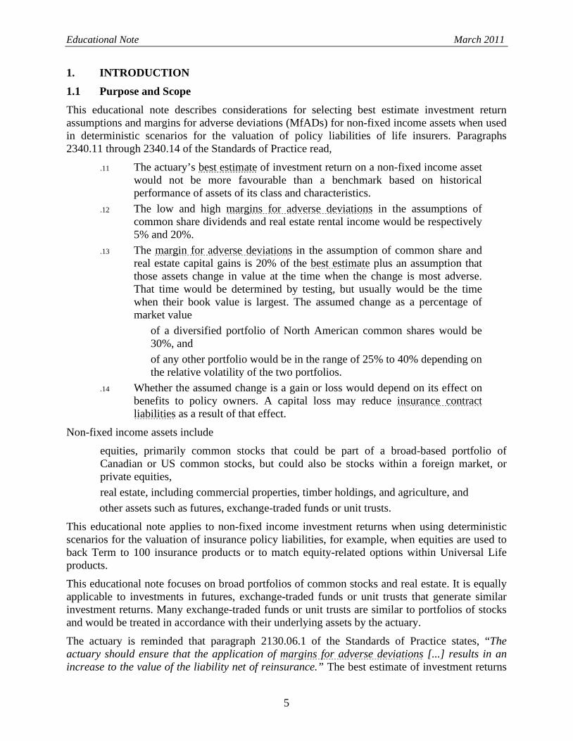
3.3 Investment Expenses No allowance would be made for investment expenses in determining the historical benchmark returns. Assumptions for investment expenses and associated MfADs would be explicitly determined based on guidance provided in other educational notes. Assumptions for management expense and brokerage fees would be based on actual company experience or contractual agreements. The table below presents an example of the development of the investment assumptions net of investment expenses and fees.
Table 3: Investment Expense Assumptions Expected Valuation*
Benchmark Return 9.00% 7.20%
Investment Expenses -0.20% -0.24%
Management Fees -1.25% -1.25%
Net Return 7.55% 5.71%
* Market shift applied separately.
3.4 Multiple Non-Fixed Income Assets Care would be taken when a company invests in several classes of non-fixed assets. This could apply to Term to 100 or Long-Term Care products that are backed by several different portfolios of assets, while for Universal Life products, policyholders may have several funds from which to choose.
For general account non-fixed income assets, the proportion of each of the different classes may be set by the actuary based on the investment mix as of the valuation date as well as a long-term

Educational Note March 2011
13
view of the investment strategy. As an alternative, the actuary may define reinvestment and disinvestment rules and allow the mix by asset class to emerge through the CALM modelling. The actuary would ensure that the projected mix of assets meets any limitations on the proportion of assets invested in one asset class, and in all other ways is consistent with the company’s investment policy.
For Universal Life products, the actuary may create a blended return using some or all of the equity-linked funds based on assumptions about policyholder fund mixes in future years. A blended assumption implicitly assumes that assets will be rebalanced to maintain a similar mix of assets in future years. Alternatively, the actuary may model each equity fund separately and make explicit assumptions about fund transfers made by policyholders to achieve a target mix in the future years. The actuary is referred to the November 2006 Draft Educational Note on Valuation of Universal Life Policy Liabilities for additional considerations.
3.5 Allowance for Recent Market Experience A related issue that receives a significant amount of discussion is whether the investment return assumption may explicitly allow for recent market experience and reflect an assumption that following a period of significant appreciation, a future correction is more likely and vice versa. This is a form of state dependent models so such economic assumptions are reasonable provided the resulting best estimate investment return does not exceed the historical benchmark return.
Appendix C: Illustration of Projected Equity Returns has been reproduced from the November 2006 Educational Note on Use of Actuarial Judgment in Setting Assumptions and Margins for Adverse Deviations. It illustrates different approaches that the actuary may take in setting the best estimate equity return assumption at successive valuation dates, and the effect that changes in equity markets between those valuation dates may have on the assumption and the policy liabilities.
3.6 Frequency of Updates The benchmark returns would be updated at least annually, ideally at the end of the same month, to provide consistency in the historical benchmark returns. The lag between the valuation date and calculation date would be reasonably short and would not exceed 12 months in any event. A lag exceeding 12 months would not adequately recognize recent changes in market values, particularly during periods of economic downturns. Table 4 below illustrates the quarterly changes in the S&P/TSX Composite index from December 2006 to December 2008. Although the historical benchmark is based on an average of returns for a period exceeding 50 years, the benchmark return may change by over 100 bps during periods of sustained economic downturns such as that experienced during the last half of 2008.

Educational Note March 2011
14
Table 4: Quarterly Changes in Historical Benchmark Return S&P/TSX
Composite Index Period Jan 1956 to Date Dec 2006 9.97% Mar 2007 9.98% June 2007 10.06% Sep 2007 10.05% Dec 2007 9.97% Mar 2008 9.86% June 2008 9.99% Sep 2008 9.52% Dec 2008 8.95% 4. COMMON SHARE DIVIDEND AND REAL ESTATE RENTAL INCOME Common share dividends and real estate rental income are important components of non-fixed income investment returns. There needs to be an appropriate balance between the dividend and capital appreciation components of the investment return assumption. Too much weight to the dividend component may overstate the value of the tax preferred status of Canadian corporate dividends or understate the resulting provisions for adverse deviations. Too little weight may understate the cash flows related to dividends. The sections provide guidance on the proportion of the total return that will be allocated to dividends or rental income.
4.1 Dividend Yields The dividend yield reported by the S&P/TSX Composite index is defined as the expected dividend payable for the next 12 months as a percentage of the market value of the index. When using deterministic scenarios, the historical dividend yield would be determined as the arithmetic average of the historical dividend yields of the selected benchmark over the selected historical period.
Generally, the most appropriate historical period to determine the best estimate of dividend yield is the longest possible period because it provides for a more stable projection. The actuary would assume a higher or lower dividend yield if this is a more appropriate representation of future dividend patterns.
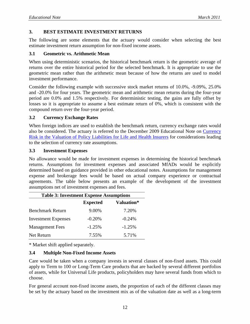
Graph 3 shows the historical dividend yields for the S&P/TSX Composite index from January 1956 to December 2008. From 1956 to 1971, dividend yields averaged between 3.0% and 4.0%. From 1974 to 1982, dividend yields increased in response to rising interest rates. The yields returned to historical levels from 1983 to 1991. From 1991 to 2004, dividend yields decreased due to the effect of high-tech stocks with no corporate dividends. Since 2005, the inclusion of Income Trusts in the S&P/TSX Composite index has increased the published dividend yield.
Educational Note March 2011
15
Graph 3
Table 5 summarizes the actual historical dividend yields for the three periods, January 1956 to December 2008, January 1979 to December 2008 and January 1991 to December 2004. Over the longest period, the dividend yield averaged just over 3.0% of the price index. For the more recent period from January 1979 to December 2008, the historical average decreased to 2.72%. For the period just prior to the inclusion of income trusts from January 1991 to December 2004, the dividend yield average was lowest at 2.04%.
Table 5: S&P/TSX Composite Index Month-end Dividend Yields
Jan 1956 to Dec 2008
Jan 1979 to Dec 2008
Jan 1991 to Dec 2004
Average 3.09 2.72 2.04
Standard Deviation 0.95 0.98 0.63 When income trusts were added to the S&P/TSX Composite index, the TSX developed an Equity index that excluded the income trusts. The graph below compares the dividend yields of the two indices, Composite and Equity. The dividend yields were estimated retrospectively using the sum of the monthly differences of the changes of the total return index less the changes in the price index. The graph below illustrates that the increase in the dividend yield from late 2005 to mid 2008s was primarily related to the introduction of income trusts. However, the effect on the historical dividend yield has not been material at less than 0.08% of the price index.
S&P/TSX Composite IndexDividend Yield from Jan 1956 to Dec 2008
0.0%
1.0%
2.0%
3.0%
4.0%
5.0%
6.0%
7.0%
1956 1961 1966 1971 1976 1981 1986 1991 1996 2001 2006Year
Divi
dend
Yie
ld
DividendYield

Educational Note March 2011
16
Graph 4
A similar approach would generally be used to determine the best estimate dividend return for other benchmarks.
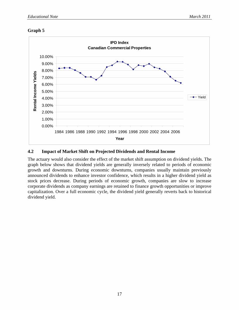
For real estate investments, rental income yields are more stable than dividend yields for equity investments since rental income comprises a greater proportion of the total return for real estate and real estate properties are typically reappraised on an annual basis. The graph below illustrates the Canadian rental income as a percentage of the IPD price index for the period January 1984 to December 2008. The rental income has varied from about 6.0% to 9.0% per year over the period. The average rental income yield over this period was 8.0% with a standard deviation of 0.9%.
S&P/TSX Dividend YieldsComposite vs. Equity Indices
-
0.50
1.00
1.50
2.00
2.50
3.00
3.50
4.00
1996 1998 2000 2002 2004 2006 2008
Year
Div
iden
d Y
ield
EquityIndexCompositeIndex
Educational Note March 2011
17
Graph 5
4.2 Impact of Market Shift on Projected Dividends and Rental Income The actuary would also consider the effect of the market shift assumption on dividend yields. The graph below shows that dividend yields are generally inversely related to periods of economic growth and downturns. During economic downturns, companies usually maintain previously announced dividends to enhance investor confidence, which results in a higher dividend yield as stock prices decrease. During periods of economic growth, companies are slow to increase corporate dividends as company earnings are retained to finance growth opportunities or improve capitalization. Over a full economic cycle, the dividend yield generally reverts back to historical dividend yield.
IPD Index Canadian Commercial Properties
0.00%
1.00%
2.00%
3.00%
4.00%
5.00%
6.00%
7.00%
8.00%
9.00%
10.00%
1984 1986 1988 1990 1992 1994 1996 1998 2000 2002 2004 2006
Year
Ren
tal I
ncom
e Yi
elds
Yield

Educational Note March 2011
18
Graph 6
The dividend component is usually expressed as a constant percentage of the market value of the benchmark, which proportionately decreases the projected dividend income when the market shift assumption is applied. This is a reasonably conservative approach that recognizes that dividend yields will return to historical levels over a full economic cycle.
Alternatively, an assumption that the projected dividends could be assumed to remain level or the reduction is less than a proportional decrease (i.e., the dividend percentage increases) at the time of the market shift may be selected. However, the actuary would ensure that the total return, including the dividend yield after the market shift, would not be more favorable than the historical benchmark return.
Similar considerations apply to rental income for real estate investments.
4.3 Taxation of Dividends and Rental Income In Canada, Canadian corporate dividends are non-taxable when received by another Canadian corporation.
Prior to 2005, the dividend income for S&P/TSX Composite index was fully non-taxable. Starting in late 2005, income trusts were phased into the S&P/TSX Composite index. While Income Trusts have increased the published dividend yield, most of the increase is not from pure dividends but rather from distribution of the normal income of the income trusts, which is fully taxable.
Using data from the Composite and Equity indices, the non-taxable portion of the dividend yield can be estimated for the S&P/TSX index. As of September 30, 2009, the Equity index represented about 92.5% of the total market value of the Composite (160 of the 204 companies in the Composite). The Equity index dividend yield was 2.47% or about 85% of the 2.90% dividend yield of the Composite index. Thus, about 78% (92.5% times 85%) of the current dividend yield is non-taxable.
S&P/TSX Composite Index Dividend Yields vs. Annualized Total Returns
-75%
-50%
-25%
0%
25%
50%
75%
1956 1961 1966 1971 1976 1981 1986 1991 1996 2001 2006
Year
Annu
aliz
ed T
otal
Ret
urns
0%
1%
2%
3%
4%
5%
6%
Divi
dend
Yie
lds
AnnualizedReturn
DividendYield

Educational Note March 2011
19
The taxable portion of the dividend yield is anticipated to change by 2011 as income tax changes for income trusts announced on October 31, 2006 become effective. The actuary would take into consideration the impact of the proposed changes to tax regulations on income trusts and its associated distributions of taxable and non-taxable income.
Caution would be used when setting the dividend assumption for foreign investments. The dividends likely do not generate the same tax-free status as Canadian corporate dividends and if they are being used to back Canadian liabilities, they are likely subject to withholding taxes, which may not generate a Canadian tax offset. If such is the case, the dividend component of the return would be reduced accordingly.
For real estate investments, the actuary would reflect tax-timing differences that may arise between statutory and taxable income.
4.4 Margins for Adverse Deviations Paragraph 2340.12 of the Standards of Practice provides that the low and high margins in the assumptions of common share dividends and real estate rental income are 5% and 20%. The actuary would review the November 2006 Educational Note on Use of Actuarial Judgment in Setting Assumptions and Margins for Adverse Deviations for considerations leading to the selection of a MfAD.
5. MARGINS FOR ADVERSE DEVIATIONS FOR COMMON SHARE AND REAL ESTATE CAPITAL GAINS
For the assumption of common share and real estate capital gains, the MfAD is 20% of the best estimate investment return. The market shift as a percentage of market value of a diversified portfolio of North American common shares is 30%, and of any other portfolio is in the range of 25% to 40% depending on the relative volatility of the two portfolios. Whether the assumed change is a gain or loss depends on its effect on benefits to policyholders. Usually, a capital loss increases policy liabilities as a result of that effect, however, in some situations, a capital gain may increase policy liabilities.
5.1 Relative Volatility The volatility for a benchmark would usually be determined as the standard deviation of the monthly total returns. Due to the relative stability of the dividend component of most equity indices, the volatility of the price index is often very close to the volatility of the total return index and may be used when total return data are unavailable. For example, for the period from January 1956 to December 2008, the annualized volatility of the S&P/TSX Composite Price index was 15.56% whereas it was 15.50% for the Total Return index. Similarly, for the S&P 500 index, the values were 14.59% for the Price index and 14.60% for the Total Return index.
5.2 Diversified North American Portfolio For a diversified portfolio of North American common shares, the MfAD is 20% of the capital gains and a 30% assumed market shift. Generally, the MfADs for scenario-tested assumptions, including the market shift, would be selected to approximate a CTE(60) to CTE(80) policy liability.
Graphs 7 and 8 below compare the deterministic valuation assumptions for North American equities to projected equity returns determined using stochastic equity models for the S&P/TSX Composite index. The graphs were developed using historical data for the S&P/TSX Composite

Educational Note March 2011
20
index from January 1956 to December 2008 (see appendix D for the deterministic valuation assumptions and log normal (LN) and regime-switching log normal (RSLN) parameters).
The projected annual equity returns for the deterministic valuation assumptions are compared to the CTE(40), CTE(60) and CTE(80) level returns for the stochastic models. The graphs illustrate that the deterministic assumptions approximate CTE(60) level returns generated by a lognormal stochastic model, but are slightly higher than the CTE(60) returns compared to a regime switching lognormal model. Since the CTE(60) level does not provide a margin for parameter uncertainty, basis risk or other model risks (dynamic lapses), the actuary would consider increasing the MfAD. A decrease to the historical benchmark return in the range of 0.00% to 1.50% would result in projected equity returns in the range of CTE(60) to CTE(80) for varying projection periods.
Graph 7
S&P/TSX Composite Index LN Model
-4.0%
-2.0%
0.0%
2.0%
4.0%
6.0%
8.0%
10.0%
12.0%
0 5 10 15 20 25 30 35 40 45 50
Projection Period
Proj
ecte
d Av
erag
e An
nual
Ret
urns
DeterministicCTE(40)CTE(60)CTE(80)

Educational Note March 2011
21
Graph 8
5.3 Selection of Market Shift Assumptions For equity portfolios other than well-diversified North American portfolios, the MfAD is 20% of the capital gains and an assumed market shift in the range of 25% to 40% depending on the relative volatility of the portfolio to a diversified portfolio of North American common shares.
The following table illustrates that the volatility for the selected benchmarks described in section 2 ranges from approximately 15% to 35%. For a diversified portfolio of North American common shares, such as the S&P/TSX Composite index and the S&P 500, the annualized volatility is approximately 15% while a portfolio of equities invested in high-tech or foreign markets ranges from 17% to 35%.
S&P/TSX Composite IndexRSLN Model
-4.0%
-2.0%
0.0%
2.0%
4.0%
6.0%
8.0%
10.0%
12.0%
0 5 10 15 20 25 30 35 40 45 50
Projection Period
Proj
ecte
d Av
erag
e An
nual
Ret
urns
DeterministicCTE(40)CTE(60)CTE(80)

Educational Note March 2011
22
Table 6: Equity Benchmark (Total Return – Local Currency – December 2008)
Benchmark Data From Frequency Annualized Geometric
Mean
Annualized Volatility
S&P/TSX Composite Jan. 1956 Monthly 8.97% 15.56%
S&P 500 Jan. 1956 Monthly 9.28% 14.59%
NASDAQ Feb. 1971* Monthly 7.75% 21.86%
FTSE All-Shares May 1962* Monthly 8.77% 19.27%
MSCI EAFE Jan. 1970 Monthly 9.66% 16.85%
Nikkei 225 Feb. 1970* Monthly 3.85% 19.15%
Hang Seng Dec. 1969* Monthly 12.66% 34.20%
* The data series combines information from a price and total return series.
The market shift assumption for a non-North American benchmark would be based on the directional impact of the relative volatilities for the benchmark to the range of 25% to 40% rather than being directly proportional to the North American equity market volatility of 15%. Table 7 below illustrates the selection of the market shift assumption for different investment classes with volatilities ranging from 10% to 30%.
Table 7: Relative Volatilities and Assumed Market Shift Investment Class Volatility Assumed Market Shift
Directly Proportional
Directional Impact
Balanced 10% 20% 25%
Dividend Income 12% 25% 27.5% Broad-Based Diversified North American 15% 30% 30%
Intermediate Risk 20% 40% 33.3%
Aggressive or Foreign 30% 60% 40% When the annualized volatility is greater than 20%, the actuary may consider selecting a lower benchmark return or a higher market shift assumption so that the projected returns are consistent with returns at a CTE(60) to CTE(80) level as discussed below.
5.4 Net Risk Premiums The availability of reliable historical data of a sufficiently long period or credibility is unlikely for sub-sectors of established markets (for example, equity sub-indices or timberland properties), less developed geographical markets or other types of non-fixed income assets. The returns and volatilities for these markets or assets may be higher than those observed for equities in the same jurisdiction due to the smaller capitalization of the markets, less diversification, higher risk and shorter observation periods. It would be reasonable to select returns higher than those observed for equities in the same jurisdiction as long as higher volatility, MfADs or market shifts are
Educational Note March 2011
23
assumed for the markets or assets in question. Recognizing the uncertainty around the data, the actuary would be cautioned against assuming that a significant net risk premium can be earned over the risk-free interest rates in the base scenario. In any event, the implied net risk premium assumed by the actuary, reduced by the chosen MfAD, would not exceed the equivalent result assumed for equities in a) the same jurisdiction when appropriate benchmarks are available, or b) Canada, when appropriate benchmarks are not available in the same jurisdiction.
Appendix E provides a detailed example of the net risk premium calculation for equities in a market with unreliable historical experience. The actuary initially uses available data and chooses appropriate MfADs for dividend income and capital growth, including the market shift assumption. However, the resulting net risk premium over risk-free rates is 4.22% compared to 2.00% for Canada. Using this calculation, the actuary would then reduce the best estimate capital growth assumption from 17.0% to 14.08% (or alternatively increase the MfAD), which reduces the resulting net risk premium to 2.00%. Therefore, the actuary would not use a capital growth assumption in excess of 14.08% for this asset portfolio.
Note that the net return “cap” referred to in the appendix is based on the Canadian Equity benchmark, not on the net returns that the actuary assumes for an existing Canadian Equity portfolio. For example, suppose the Canadian benchmark return is 10%, but the actuary selects a 9% return for a portfolio of Canadian assets (along with the prescribed 30% shift). The “net risk premium” benchmark would be based on the original 10% benchmark and not the actuary’s assumption of 9%. In this way, every company will have the same benchmark for assets with unreliable historical data.
Similar considerations would apply to net risk premium after margins for investments in sub-sectors of established markets (for example, equity sub-indices or timberland properties) less developed geographical markets, or other types of non-fixed income assets.
5.5 Higher Relative Volatilities When the annualized volatility is greater than 20%, a market shift assumption greater than 40% may be required to approximate a CTE(60) to CTE(80) liability. As an example, the volatility of the Hang Seng index is approximately 35%, which is significantly greater than a volatility of 15% for a well-diversified North American index. Graphs 9 and 10 below show that the projected average annual returns of the deterministic valuation assumptions for the Hang Seng index with a 20% MfAD and a 40% market shift (shown as deterministic A) is generally in the range of CTE(40) to CTE(50), and would therefore be inconsistent with a CTE(60) to CTE(80) policy liability. On the other hand, if the deterministic assumption is developed with a 65% market shift (shown as deterministic B), then the returns generated are now in the range of CTE(60) to CTE(65) and, therefore, would be appropriate.

Educational Note March 2011
24
Graph 9
Graph 10
Hang Seng Index LN Model
-4.0%
-2.0%
0.0%
2.0%
4.0%
6.0%
8.0%
10.0%
12.0%
0 5 10 15 20 25 30 35 40 45 50
Projection Period
Proj
ect A
vera
ge A
nnua
l Ret
urns
Deterministic ADeterministic BCTE(40)CTE(60)CTE(80)
Hang Seng Index RSLN Model
-4.0%
-2.0%
0.0%
2.0%
4.0%
6.0%
8.0%
10.0%
12.0%
0 5 10 15 20 25 30 35 40 45 50
Projection Period
Proj
ecte
d Av
erag
e An
nual
Ret
urns
Deterministic ADeterministic BCTE(40)CTE(60)CTE(80)

Educational Note March 2011
25
In order to select a market shift assumption that is higher than the “high” margin of 40%, the actuary would follow the approach outlined in subsection 1330 of the Standards of Practice. In any event, the net risk premiums after margin would still be less than those available for equities in the same jurisdiction or in the Canadian market, as appropriate.
5.6 Real Estate Market Shifts For real estate indices, the annualized volatility is approximately 5%, which is significantly lower than that for equity funds. Since real estate values for the ICREIM/IPD and NCREIF indices are based on appraisal values rather than actual transactions, the resulting returns are inherently smoothed, which lowers the volatility of the indices. CLIFR believes that a minimum market shift assumption of 25% is appropriate for real estate investments.
Table 8: Real Estate Benchmark (Total Return – Local Currency – December 2008)
Benchmark Data From Frequency Annualized Geometric
Mean
Annualized Volatility
ICREIM/IPD (Canada) Jan. 1985 Annual 9.43% 7.08%
NCREIF (US) Jan. 1978 Quarterly 9.71% 3.87% 5.7 Timing of Market Shifts The actuary would perform tests to assess when the timing of the market shift has the largest increase in the policy liability. The largest increase in the policy liability usually occurs when the projected value of the non-fixed income assets is largest. For mature blocks of Universal Life business with significant amounts of equity-linked investment options, the market shift will usually be assumed to occur as the cash values start to decrease at a time relatively close to the valuation date. For Term to 100 or Long-Term Care policies, the assets backing liabilities may increase for many years before declining, so a relatively long period may be required.
Policies with different risk characteristics would be considered in aggregate to evaluate the risk exposure to the insurance company. As the actual investment experience is not likely to differ between non-fixed investments in different asset segments, a market shift determined in aggregate better captures the aggregate risk. The actuary would review the September 2003 Educational Note on Aggregation and Allocation of Policy Liabilities for additional considerations.
5.8 Increase or Decrease for Market Shifts Whether the assumed market shift is an increase or decrease depends on its effect on benefits to policyholders. A decrease market value usually increases the policy liabilities for universal life or Term to 100 businesses since the net amount at risk increases or additional assets will be required to support the liabilities. However, in some situations, an increase in market values will increase policy liabilities. For example, for accumulation annuities with guaranteed annuity purchase rates, an increase in the account values just prior to annuitization would increase the guaranteed value of annuity payments.
Policies with different risk characteristics would be considered in aggregate to evaluate the risk exposure to the insurance company. The actuary would review the September 2003 Educational Note on Aggregation and Allocation of Policy Liabilities for additional considerations.

Educational Note March 2011
26
5.9 Other Considerations The actuary would review the November 2006 Educational Note on Use of Actuarial Judgment in Setting Assumptions and Margins for Adverse Deviations for considerations leading to the selection of a MfAD.
For practical purposes, the market shift assumption is sometimes expressed as an equivalent level deduction to the expected return based on the average duration for the liabilities backed by the equity investments. Table 9 below illustrates the resulting net annualized returns at specific durations using this approach. Generally, the net annualized returns for earlier durations are overstated while the net annualized returns are understated at later durations. For example, the equivalent level annualized return for a term of 30 years is 5.89%, which is greater than the equivalent level return of 3.40% for a duration of 10 years. The actuary would use caution when using this approach to ensure that this approach does not overstate the expected return assumption for short-term liabilities.
Table 9: Equivalent Level Market Shift Assumptions
Duration BE Return 20% MfAD Equivalent
Level Market Shift
Equivalent Level Annual
Return 5 8.95% -1.79% -7.38% -0.22%
10 8.95% -1.79% -3.75% 3.40%
15 8.95% -1.79% -2.52% 4.64%
20 8.95% -1.79% -1.89% 5.26%
25 8.95% -1.79% -1.52% 5.64%
30 8.95% -1.79% -1.27% 5.89%
35 8.95% -1.79% -1.09% 6.07%
40 8.95% -1.79% -0.95% 6.20%
45 8.95% -1.79% -0.85% 6.31%
50 8.95% -1.79% -0.76% 6.39%

Educational Note March 2011
27
APPENDIX A: DESCRIPTIONS OF BENCHMARK INDICES – EQUITIES 1. Canadian Equities – S&P/TSX Composite
Overview The S&P/TSX Composite index is maintained by Standard and Poor’s and the Toronto Stock Exchange. It is regarded as a good general indicator of stock price movements for Canada. The index is market capitalization weighted and includes common stocks and income trust units.
Total return information is available monthly back to 1956. The Canadian data prior to 1956 are limited and do not provide the same market coverage. They may also be considered more volatile due to events such as the Great Depression in the 1930s and the fiscal restraints imposed during World War II. Therefore, for practical considerations, January 1956 is used as the starting point of the historical period to establish historical returns for Canadian equities.
Although this is a broad-based index, the financial, energy and material sectors are predominant as they represent almost 80% of the total market capitalization of the index.
History This index replaced the TSE 300 Composite index on May 1, 2002. On that date, its constituents and the index calculation method were exactly the same as before. With ongoing quarterly revisions, companies that do not meet size and liquidity requirements are dropped from the index while newly qualifying ones are brought in. Since May 2002, the number of companies has dropped from 300, and was 269 as of September of 2007. The number of companies had dropped to just over 200 until income trusts were added in the fall of 2005.
The TSE 300 composite price index was created in 1977, replacing the old Toronto Stock Exchange indices, with a base level of 1,000 as of 1975. The new indices were calculated on a monthly basis back to 1956 and on a daily basis back to 1971. Through the years the index consisted of a sample of 300 companies, though the companies that comprised the index varied from year to year. Stocks were dropped when they no longer met exchange requirements.
Data Series The monthly total return data series are available from the Scotia Capital Handbook (up to 2005) and Bloomberg (post 2005).
The Common Stock index values in the CIA’s Canadian Economic Statistics for 1957 and later years are based on the December month-end values for the Total Return version of this index.
Other Notes Constituents of the S&P/TSX Composite are also members of either the S&P/TSX Equity indices (the S&P/TSX Equity, the S&P/TSX Equity 60, and the S&P/TSX Equity Completion) or the suite of indices which include income trusts (the S&P/TSX Income Trust, the S&P/TSX Capped REIT, and the S&P/TSX Capped Energy Trust), or both. The S&P/TSX SmallCap index is a completely separate index from the S&P/TSX Composite family of indices.
References http://www2.standardandpoors.com/spf/pdf/index/SP_TSX_Canadian_Indices_Methodology_Web.pdf

Educational Note March 2011
28
2. U.S. Equities – S&P 500 Overview The S&P 500 index is considered to be an appropriate guide to returns on most well-diversified portfolios of publicly traded American stock. Widely regarded as the best single gauge of the U.S. equities market, this world-renowned index includes 500 leading companies in leading industries of the U.S. economy. The index is market capitalization weighted and covers approximately 75% of the total U.S. equity market.
The components of the S&P 500 are selected by committee. The committee selects the companies in the S&P 500 so they are representative of the industries in the U.S. economy. In addition, companies that do not trade publicly (such as those that are privately or mutually held) and stocks that do not have sufficient liquidity are not in the index.
History The S&P 500 index was computed back to 1928. The S&P 500’s base period is 1941 to 1943. The actual total market value of the index during the base period has been set equal to a value of 10.
On March 4, 1957 the S&P 500 daily composite stock price index was launched. It is based on 500 stocks consisting of 425 industrials, 15 rails and 60 utilities, computed at one-minute intervals and published as of each hour in S&P’s Corporation Records Service. Daily High, Low and Close of the indices are published in the weekly The Outlook and the monthly Current Statistics. Components of the daily 90 stock indices were standardized with the 500 stock index as of March 1, 1957.
On October 9, 2007, the index closed at an all-time high of 1,565; the decline from this peak signalled the beginning of the more recent financial crisis. At the end of December 2008, the index closed at 903.
Data Series The monthly total return data series are available from Bloomberg. This data series goes all the way back to 1928.
The annual total returns of the S&P500, in U.S. and Canadian dollars, are available in the CIA’s Canadian Economic Statistics for 1938 and later years.
References http://www2.standardandpoors.com/spf/pdf/index/SP_500_Factsheet.pdf
http://en.wikipedia.org/wiki/S%26P_500
http://www2.standardandpoors.com/spf/pdf/index/SP500_Internal_Records_Timeline_Web.pdf
3. U.S. Equities – NASDAQ Composite Overview The NASDAQ Composite index is a market capitalization weighted index of all of the common stocks and similar securities (e.g., American Depositary Receipts (ADR), limited partnership interests, etc.) listed on the NASDAQ stock market. It has over 3,000 components. It is highly followed in the U.S. as an indicator of the performance of stocks of technology companies and growth companies. Since both U.S. and non-U.S. companies are listed on the NASDAQ stock market, the index is not exclusively a U.S. index.

Educational Note March 2011
29
History On February 5, 1971, the NASDAQ Composite index began with a base of 100.00. On March 10, 2000, the index closed at an all-time high of 5,049; the decline from this peak signalled the beginning of the end of the technology sector bubble. At the end of December 2008, the index closed at 1,577.
Data Series The monthly total return data series is available from Bloomberg, which is available since inception of the index.
The index is not provided in the CIA’s Canadian Economic Statistics.
Other Notes
Launched in January 1985, the NASDAQ-100 index represents the largest non-financial domestic and international securities listed on the NASDAQ Stock Market based on market capitalization. The NASDAQ-100 index is calculated under a modified capitalization-weighted methodology. The methodology is expected to retain in general the economic attributes of capitalization weighting while providing enhanced diversification. To accomplish this, NASDAQ will review the composition of the NASDAQ-100 index on a quarterly basis and adjust the weightings of index components using a proprietary algorithm, if certain pre-established weight distribution requirements are not met.
References http://en.wikipedia.org/wiki/Nasdaq_Composite
http://dynamic.nasdaq.com/dynamic/nasdaq100_activity.stm
4. Foreign Equities – UK Overview The FTSE All-Share is a market capitalization weighted index representing the performance of all eligible companies listed on the London Stock Exchange’s main market which pass screening for size and liquidity. Today the FTSE All-Share index represents approximately 98% of the UK’s market capitalization.
History The FTSE All-Share index was originally called the FT Actuaries All-Share index at its inception back in 1962. The index was then enhanced with the addition of two new sub-indices, namely the FTSE 100 and FTSE 250 in January 1984 and October 1992 respectively.
Prior to the launch in 1962, the FT30 index was the barometer of the investor sentiment. It is based on the share prices of 30 British companies from a wide range of industry. Similar to the Dow Jones Industrial Average, this index is using a price weighted methodology.
Data Series The monthly total return data series is only available from December 31, 1985 on Bloomberg. Prior to this date, only price return information (i.e., ignores the return earned from dividends) is available. Using the price index is reasonable for calculating the volatility of the FTSE All-Share. However, it would be conservative for determining the benchmark return.
The index is not provided in the CIA’s Canadian Economic Statistics.
Educational Note March 2011
30
Other Notes
The All-Share index can be broken down into a smaller family of indices,
FTSE 100 which comprises the largest 100 companies in the FTSE All-Share index,
FTSE 250 which comprises the next largest 250 (Mid-Cap) companies in the FTSE All-Share index, and
FTSE Small Cap which comprises the companies within the FTSE All-Share index that are not large enough to be constituents of the FTSE 100 and FTSE 250 indices.
The indices are only available from 1984.
The MCSI-UK index may also be considered as a broad-based index for the U.K. equity market. The index values are correlated at 99% with the FTSE All-Share index. The total return information for this index has been calculated since December 31, 1969 and can be retrieved from the MSCI website.
References http://www.ftse.com/Indices/UK_Indices/Downloads/FTSE_All-Share_Index_Factsheet.pdf
5. Foreign Equities – MSCI EAFE Overview The MSCI EAFE index (Europe, Australasia, and Far East) is a free float-adjusted market capitalization index that is designed to measure the equity market performance of developed markets, excluding the U.S. and Canada. Investment returns are typically expressed in U.S. dollars. MSCI aims to include in its international index 85% of the free float-adjusted market capitalization in each industry group, within each country.
History The index has been calculated since December 31, 1969, making it one of the oldest truly international stock indices. It is one of the most common benchmarks for foreign stock funds.
Recently, the weights of the various regions were approximately
40–45% for Europe (excluding United Kingdom),
20–25% for United Kingdom,
20–25% for Japan, and
8–12% for Australasia (excluding Japan).
Since 2007, the MSCI EAFE index consists of the following 21 developed market country indices: Australia, Austria, Belgium, Denmark, Finland, France, Germany, Greece, Hong Kong, Ireland, Italy, Japan, the Netherlands, New Zealand, Norway, Portugal, Singapore, Spain, Sweden, Switzerland, and the United Kingdom. These indices were calculated retroactively back to 1969.
In the mid 1990s, MSCI introduced indices for emerging markets, such as the Philippines, China, Peru, etc. The indices were calculated retroactively back to 1992.
Data Series The monthly total return data series is available from the MSCI website: http://www.mscibarra.com/products/indices/equity/levels.jsp. Similar data is also available through Bloomberg.

Educational Note March 2011
31
The index is not provided in the CIA’s Canadian Economic Statistics.
References http://www.mscibarra.com/products/indices/international_equity_indices/definitions.html
http://en.wikipedia.org/wiki/MSCI_EAFE
6. Foreign Equities – Japanese Overview Nikkei 225 Average is a stock market index for the Tokyo Stock Exchange (TSE). It is the most widely quoted average of Japanese equities. Similar to the Dow Jones Industrial Average, it is a price-weighted average index and its components are reviewed once a year. The 225 components of the Nikkei 225 are among the most actively traded issues on the first section of the TSE.
History The index has been calculated daily since September 7, 1950. The Nikkei 225 hit its all-time high on December 29, 1989, during the peak of the Japanese asset price bubble, when it closed at 38,916. On July 9, 2007, prior to the start of the most recent financial crisis, the index closed at a high of 18,262. At the end of December 2008, the index closed at 8,860.
Data Series The monthly total return data series is only available from December 31, 1969 on Bloomberg.
Other Notes TOPIX may also be considered as a broad-based index for the Japanese equity market. TOPIX is the acronym for the TOkyo stock Price IndeX. The index values are available since 1968. It covers all the companies on the first section of the Tokyo Stock Exchange. There are approx 1,700 companies listed on the first section of the TSE. The TOPIX index values are correlated at 98% with the Nikkei 225.
As well, the MCSI-Japan index is another index that could be considered. The index values are correlated at 94% with the Nikkei 225.
The total return information for this index has been calculated since December 31, 1969 and can be retrieved from the MSCI website.
References http://en.wikipedia.org/wiki/Nikkei_225
http://www.finfacts.com/Private/curency/nikkei225performance.htm
http://www.tse.or.jp/english/market/topix/history/index.html
7. Foreign Equities – Hong Kong Overview The Hang Seng index (HSI) is a free float-adjusted market capitalization-weighted stock market index in Hong Kong. It is used to record and monitor daily changes of the largest companies of the Stock Exchange of Hong Kong (SEHK) and is the main indicator of the overall market performance in Hong Kong.

Educational Note March 2011
32
Only companies with a primary listing on the Main Board of the SEHK are eligible as constituents. Mainland enterprises that have H-share listing in Hong Kong will be eligible for inclusion in the HSI when they meet various requirements.
History The HSI is one of the earliest stock market indices in Hong Kong. It was publicly launched on November 24, 1969. When the HSI was first published, its base of 100 points was set equivalent to the stocks’ total value as of the market close on July 31, 1964. The HSI closed above the 10,000 point milestone for the first time in its history on December 10, 1993, and, 13 years later, closed above the 20,000 point milestone on December 28, 2006. It closed at an all-time high (31,368) on October 30, 2007. At the end of December 2008, the index closed at 17,251.
Data Series The monthly total return data series is only available from November 30, 2004 on Bloomberg. Prior to this date, only price return information is available going back to the inception of the index.
Other Notes The MCSI – Hong Kong index may also be considered as a broad-based index for the Hong Kong market. The index values are correlated at 99% with the HSI. The total return information for this index has been calculated since December 31, 1969 and can be retrieved from the MSCI website.
References http://en.wikipedia.org/wiki/Hang_Seng_Index

Educational Note March 2011
33
APPENDIX B: DESCRIPTIONS OF BENCHMARK INDICES – REAL ESTATE 1. Canadian Real Estate – ICREIM/IPD Canada Overview The index is maintained by the Investment Property Databank (IPD). IPD is a global information business, dedicated to the objective measurement of commercial real estate performance. They operate in over 20 countries including most of Europe, the US, Canada, South Africa, Australia, New Zealand and Japan. Their indices are also the basis for the developing commercial property derivatives market.
The index is composed of data received from institutional owners of directly held properties. The data are from standing properties only and therefore exclude those under construction. The index breaks down returns into the following sectors: retail, office, industrial, residential and others. It also provides separate data series for the rental income and growth component of the total return.
Since the value of real estate properties is not measured constantly, index users should be aware that the index results reflect some approximations. In 2008, the percentage of total index quarter-end capital value appraised for each quarter was as follow: 24.2% in Q1, 41.9% in Q2, 23.2% in Q3 and 81.4% in Q4. When no quarter end valuation is available, the property value is held down at the last actual valuation, adjusted only for capital expenditure or receipts. This means that the reported index movement will lag the actual market to varying degree in each sector.
As at December 2008, the ICREIM/IPD Canadian property index was based upon 2,569 properties worth $96.5 billion.
History Data were first available from Frank Russell, which produced annual information from 1985 to 1999. IPD established its service in Canada in 2002. This was done in consultation with the Institute of Commercial Real Estate Investment Managers (ICREIM). ICREIM/IPD has produced results for the Canadian market from 2000 to 2008.
Data Series The annual return data series is available for purchase through IPD. Additional details can be found at http://www.ipd.com. In addition, quarterly return data are available since January 1, 2000.
References http://www.ipd.com
2. U.S. Real Estate – NCREIF Property Overview The index is maintained by the National Council of Real Estate Investment Fiduciaries (NCREIF). NCREIF is a non-profit organization that was established to serve the institutional real estate investment community as a non-partisan collector, processor, validator and disseminator of real estate performance information. It is supported by a membership base that includes investment managers, pension plan sponsors, academicians, consultants, appraisers, accountants and other service providers who have a significant involvement in institutional estate investments.
The NCREIF is a quarterly time series measuring the investment performance of a very large pool of individual commercial real estate properties acquired in the private market for investment purposes only. All properties in the NCREIF have been acquired, at least in part, on behalf of tax-exempt

Educational Note March 2011
34
institutional investors, with the great majority being pension funds. As such, all properties are held in a fiduciary environment. The investment returns are reported on a non-leveraged basis.
NCREIF requires that properties included in the index be valued at least quarterly, either internally or externally, using standard commercial real estate appraisal methodology. Each property must be independently appraised a minimum of once every three years.
NCREIF breaks down returns into apartments, hotels, industrial properties, office buildings, and retail sectors. It also breaks down returns by regions of East, South, Midwest and West. In addition, NCREIF publishes Timberland and Farmland indices.
History The index contains data back to 1977 when it was started as a project of the Frank Russell Company. It was first published in 1981, when it was called the Frank Russell Company Property index, or FRC Property index.
In 1982, NCREIF was established and started partnering with Frank Russell Company to collect data and publish the index under joint sponsorship. In 1991, the name of the index was renamed the Russell-NCREIF Property index.
On January 1, 1995, NCREIF assumed full responsibility for the index, and it was renamed the NCREIF Property index (NPI).
In December 2004, the NPI was based upon 4,152 properties worth US$ 145.4 billion.
Data Series The quarterly total return data series are available at: http://secure.ncreif.org/ncreif.org/index.aspx. Additional data are available for purchase through NCREIF.
References http://secure.ncreif.org/public_files/Users_Guide_to_NPI.pdf
http://secure.ncreif.org/property-index-returns.aspx

Educational Note March 2011
35
APPENDIX C: ILLUSTRATION OF PROJECTED EQUITY RETURNS This appendix has been reproduced from the November 2006 Educational Note on Use of Actuarial Judgment in Setting Assumptions and Margins for Adverse Deviations.
The following examples illustrate different approaches in setting the best estimate equity return assumption on a consistent basis period to period and their implications. Similar approaches could be used for the asset volatility assumption.
The following examples assume the historical return over the last 50 years is 9.5%. The current index is at 1,000 and was 900 one period prior and 850 two periods prior.
Company A decides to set its best estimate return at this historical average and updates this each period as the historical average changes.
Company B decides to set its best estimate return at a prudent historical long-term average. This prudent long-term average is reviewed from time to time to assess its ongoing appropriateness. For this example this rate is assumed to be 8.5%.
Company C also uses a prudent long-term average as its best estimate but assumes an initial market shift by projecting each of this year and the previous two years market levels to the end of this year. The expected first-year return is set to reproduce the average of these projections. This results in a return of 7.67% for the first year and 8.5% thereafter.
Company D also uses a prudent long-term average as its best estimate but adjusts its rate for the first 25 years dependent on recent market performance. Similar to C, Company D solves for a return for the first 25 years that reproduces the average of the last three years’ actual returns projected to the same point. This results in best estimate assumptions of 8.47% for 25 years, and 8.5% thereafter.
The resultant projected levels for each company are illustrated below.
T T+1 T+2 T+3 T+5 T+10 T+25 T+50 A 1,000 1,095 1,199 1,313 1,574 2,478 9,668 93,477 B 1,000 1,085 1,177 1,277 1,504 2,261 7,687 59,086 C 1,000 1,077 1,168 1,268 1,492 2,244 7,628 58,636 D 1,000 1,085 1,177 1,276 1,501 2,254 7,628 58,636
The following year (T+1) the actual market return is 15%.
For Company A the historical long-term average (51-year geometric return) increased to 9.61%. It revised its best estimate to this return.
Company B reviewed its prudent estimate and determined no changes were required. It continued to use 8.5%.
Company C continued its previous process with no change to the 8.5%. This resulted in a return of 3.6% in year one and 8.5% thereafter.
Company D continued its previous process with no change to the 8.5%. This resulted in a return of 8.3% for 25 years and 8.5% thereafter.
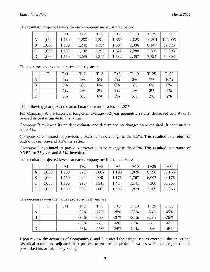
Educational Note March 2011
36
The resultant projected levels for each company are illustrated below.
T T+1 T+2 T+3 T+5 T+10 T+25 T+50 A 1,000 1,150 1,260 1,382 1,660 2,625 10,391 102,906 B 1,000 1,150 1,248 1,354 1,594 2,396 8,147 62,626 C 1,000 1,150 1,192 1,293 1,522 2,288 7,780 59,803 D 1,000 1,150 1,245 1,349 1,582 2,357 7,794 59,803
The increases over values projected last year are
T T+1 T+2 T+3 T+5 T+10 T+25 T+50 A 5% 5% 5% 5% 6% 7% 10% B 6% 6% 6% 6% 6% 6% 6% C 7% 2% 2% 2% 2% 2% 2% D 6% 6% 6% 5% 5% 2% 2%
The following year (T+2) the actual market return is a loss of 20%.
For Company A the historical long-term average (52-year geometric return) decreased to 8.94%. It revised its best estimate to this return.
Company B reviewed its prudent estimate and determined no changes were required. It continued to use 8.5%.
Company C continued its previous process with no change to the 8.5%. This resulted in a return of 31.5% in year one and 8.5% thereafter.
Company D continued its previous process with no change to the 8.5%. This resulted in a return of 9.34% for 25 years and 8.5% thereafter.
The resultant projected levels for each company are illustrated below.
T T+1 T+2 T+3 T+5 T+10 T+25 T+50 A 1,000 1,150 920 1,002 1,190 1,826 6,598 56,166 B 1,000 1,150 920 998 1,175 1,767 6,007 46,176 C 1,000 1,150 920 1,210 1,424 2,141 7,280 55,963 D 1,000 1,150 920 1,006 1,203 1,879 7,169 55,963
The decreases over the values projected last year are
T T+1 T+2 T+3 T+5 T+10 T+25 T+50 A -27% -27% -28% -30% -36% -45% B -26% -26% -26% -26% -26% -26% C -23% -6% -6% -6% -6% -6% D -26% -25% -24% -20% -8% -6%
Upon review the actuaries of Companies C and D noticed their initial return exceeded the prescribed historical return and adjusted their process to ensure the projected values were not larger than the prescribed historical, thus yielding,

Educational Note March 2011
37
for Company C, a return of 8.94% for approximately 49 years and 8.5% thereafter, and
for Company D, a return of 8.94% for approximately 49 years and 8.5% thereafter.
The resultant projected levels for each company are illustrated below.
T T+1 T+2 T+3 T+5 T+10 T+25 T+50 A 1,000 1,150 920 1,002 1,190 1,826 6,598 56,166 B 1,000 1,150 920 998 1,175 1,767 6,007 46,176 C 1,000 1,150 920 1,002 1,190 1,826 6,598 55,963 D 1,000 1,150 920 1,002 1,190 1,826 6,598 55,963
This revised approach gives a decrease over the values projected last year of
T+2 T+3 T+5 T+10 T+25 T+50 A -27% -27% -28% -30% -36% -45% B -26% -26% -26% -26% -26% -26% C -23% -22% -22% -20% -15% -6% D -26% -26% -25% -23% -15% -6%

Educational Note March 2011
38
APPENDIX D: STOCHASTIC INVESTMENT MODEL PARAMETERS 1. S&P/TSX Composite Index The model was calibrated for the period January 1956 to December 2008. For the log normal (LN) model, the parameters for the models are based on actual monthly index values. The volatilities were adjusted to meet the calibration criteria of the March 2002 Report of the CIA Task Force on Segregated Fund Investment Guarantees. For the regime-switching log normal (RSLN) model, the parameters were calibrated using a maximum likelihood estimator. No adjustment was needed to meet the segregated fund calibration criteria mentioned above. The parameters for the models are:
S&P/TSX Composite LN Parameters as of December 31, 2008
μ 8.94%
σ 15.6%
Adjusted σ 18.4%
S&P/TSX Composite RSLN Parameters as of December 31, 2008
Regime 1 Regime 2
μ 15.3% -24.8%
σ 11.8% 25.9%
p 16.4% 79.4% 2. Hang Seng Index The model was calibrated for the period November 1969 to December 2008. For the LN model, the parameters for the models are based on actual monthly index values. The volatilities were adjusted to meet the calibration criteria of the March 2002 Report of the CIA Task Force on Segregated Fund Investment Guarantees. For the RSLN model, the parameters were calibrated using a maximum likelihood estimator. No adjustment was needed to meet the segregated fund calibration criteria mentioned above. The parameters for the models are:
Hang Seng Price Index LN Parameters as of December 31, 2008
μ 12.2%
σ 34.4%
Adjusted σ 37.6%

Educational Note March 2011
39
Hang Seng Price Index RSLN Parameters as of December 31, 2008
Regime 1 Regime 2
μ 22.83% -3.61%
σ 17.88% 47.99%
p 31.79% 42.87%

Educational Note March 2011
40
APPENDIX E: EXAMPLE OF EQUITY RETURNS FOR EMERGING MARKETS This appendix illustrates how to test that the net risk premium over the risk-free interest rates for the best estimate return assumption for equities in a market with unreliable historical experience does not exceed the net risk premium implied for Canadian equities. Similar considerations would apply to net risk premium after margins for investments in sub-sectors of established markets (for example, equity sub-indices or timberland properties), less developed geographical markets, or other types of non-fixed income assets.
The attached table has been reproduced from the November 2009 Educational Note on Guidance for the 2009 Valuation of Policy Liabilities of Life Insurers. The actuary initially uses the available data to develop historical returns for capital growth and dividends for Canadian equities and the emerging market (XYZ). Data is available with a period of 50 years for Canada and limited to 20 years for XYZ. The volatilities are 22% and 37% for Canada and XYZ respectively. Then, appropriate MfADs are selected for dividend income and capital growth (including the market value shift at worst time) for each market. The risk-free rates are selected from the base scenario for CALM testing. A 10-year period was selected for the test, which reflects the mean duration of the liability cash flows for the base scenario.
For Canadian equities, the resulting net risk premium over risk-free rates is 2.00%. However, for the XYZ market, the net risk premium is 4.22%, which is in excess of the Canadian net risk premium. Recognizing this net risk premium is inappropriate given the uncertainty around the data for XYZ, the best estimate capital growth assumption would be decreased from 17.00% to 14.08%, which reduces the resulting net risk premium to the equivalent result of 2% for Canadian equities. Therefore, the capital growth rate assumption would not exceed 14.08% for this market.
The length of the projection period selected for the test will impact the calculation of the net risk premium and the resulting limit on the capital growth rate for the XYZ market. A longer projection period will generally increase the net risk premium over the risk-free interest rates where the yield curve is relatively flat for Canadian equities. However, the resulting capital growth rate for XYZ may be lower depending on the relative volatilities of the two markets.

Educational Note March 2011
41
Canada (50 yrs) XYZ (20 yrs)Historical return - capital growth (given) 9.50% 17.00% - dividends (given) 2.50% 3.00% Total 12.00% 20.00%
Risk-free rate (given) 4.00% 6.00%
Implied Spread: 8.00% 14.00%
Volatility (given - information only): 22% 37%
MfADs (given): - on dividends 10% 20% - on capital growth 20% 20% - shock (applied in year 5): 30% 40%
0 1 2 3 4 5 6 7 8 9 10Canada
Capital Growth 7.60% 7.60% 7.60% 7.60% 7.60% 7.60% 7.60% 7.60% 7.60% 7.60%Dividends 2.25% 2.25% 2.25% 2.25% 2.25% 2.25% 2.25% 2.25% 2.25% 2.25%Net Return (before shock) 9.85% 9.85% 9.85% 9.85% 9.85% 9.85% 9.85% 9.85% 9.85% 9.85%Shock 0.00% 0.00% 0.00% 0.00% -30.00% 0.00% 0.00% 0.00% 0.00% 0.00%Cumulative (after shock) 1,000.00 1,098.50 1,206.70 1,325.56 1,456.13 1,119.69 1,229.98 1,351.13 1,484.22 1,630.42 1,791.01
Net Spread over Risk Free (incl. dividends) 2.00%
XYZ (Initial, using unmodified empirical estimate of capital growth)Capital Growth 13.60% 13.60% 13.60% 13.60% 13.60% 13.60% 13.60% 13.60% 13.60% 13.60%Dividends 2.40% 2.40% 2.40% 2.40% 2.40% 2.40% 2.40% 2.40% 2.40% 2.40%Net Return (before shock) 16.00% 16.00% 16.00% 16.00% 16.00% 16.00% 16.00% 16.00% 16.00% 16.00%Shock 0.00% 0.00% 0.00% 0.00% -40.00% 0.00% 0.00% 0.00% 0.00% 0.00%Cumulative (after shock) 1,000.00 1,160.00 1,345.60 1,560.90 1,810.64 1,260.20 1,461.84 1,695.73 1,967.05 2,281.78 2,646.86
Net Spread over Risk Free (incl. dividends) 4.22%
XYZ (Revised)Revised b.e. capital growth assumption 14.08%
Capital Growth 11.26% 11.26% 11.26% 11.26% 11.26% 11.26% 11.26% 11.26% 11.26% 11.26%Dividends 2.40% 2.40% 2.40% 2.40% 2.40% 2.40% 2.40% 2.40% 2.40% 2.40%Net Return (before shock) 13.66% 13.66% 13.66% 13.66% 13.66% 13.66% 13.66% 13.66% 13.66% 13.66%Shock 0.00% 0.00% 0.00% 0.00% -40.00% 0.00% 0.00% 0.00% 0.00% 0.00%Cumulative (after shock) 1,000.00 1,136.60 1,291.87 1,468.34 1,668.92 1,138.14 1,293.61 1,470.32 1,671.17 1,899.45 2,158.92
Net Spread over Risk Free (incl. dividends) 2.00%
Test Projection
Data, Assumptions and Comments
This exhibit illustrates how the actuary might test to ensure the best estimate assumption for equity returns for a geography with unreliable historical experience. Here, the actuary initially uses what data he has and chooses appropriate MfADs for dividend income and capital growth (including the shock at worst time per SOP 2340.13).
However, the resulting 'net' risk premium over risk-free rates is 4.22% compared to 2% for Canada. Recognizing this result to be inappropriate given the uncertainty around the data, he then reduces the best estimate capital growth assumption from 17% to 14.08%, which reduces the resulting net risk premium to 2%. Therefore, he would not use a capital growth assumption in excess of 14.08% for this market.