research papers

Acta Cryst. (2018). D74, 519–530 https://doi.org/10.1107/S2059798318002425 519

Received 11 November 2017

Accepted 9 February 2018

Keywords: model building; real-space

refinement; molecular dynamics; visualization;

ISOLDE.

Supporting information: this article has

supporting information at journals.iucr.org/d

ISOLDE: a physically realistic environment formodel building into low-resolution electron-densitymaps

Tristan Ian Croll*

Cambridge Institute for Medical Research, University of Cambridge, Wellcome Trust/MRC Building, Cambridge CB2 0XY,

England. *Correspondence e-mail: tic20@cam.ac.uk

This paper introduces ISOLDE, a new software package designed to provide

an intuitive environment for high-fidelity interactive remodelling/refinement

of macromolecular models into electron-density maps. ISOLDE combines

interactive molecular-dynamics flexible fitting with modern molecular-graphics

visualization and established structural biology libraries to provide an

immersive interface wherein the model constantly acts to maintain physically

realistic conformations as the user interacts with it by directly tugging atoms

with a mouse or haptic interface or applying/removing restraints. In addition,

common validation tasks are accelerated and visualized in real time. Using the

recently described 3.8 A resolution cryo-EM structure of the eukaryotic

minichromosome maintenance (MCM) helicase complex as a case study, it is

demonstrated how ISOLDE can be used alongside other modern refinement

tools to avoid common pitfalls of low-resolution modelling and improve the

quality of the final model. A detailed analysis of changes between the initial and

final model provides a somewhat sobering insight into the dangers of relying on

a small number of validation metrics to judge the quality of a low-resolution

model.

1. Introduction

As the resolution of a crystallographic or cryo-EM data set

degrades, the challenge faced by the model builder increases

rapidly as first individual atoms, then small bonded groups and

eventually entire residues become effectively unidentifiable

from the density alone. The difficulty is further compounded

by the fact that low-resolution structures often tend to also be

large structures (Supplementary Fig. S1), with thousands or

even tens of thousands of residues to contend with. It is

unsurprising, then, that the rate of residual errors in published

structures similarly grows steeply with decreasing resolution.

This fact has long been recognized (Kleywegt & Jones, 1995),

and over the past two decades it has been common to see

3–4 A resolution structures published with outlier rates 1–2

orders of magnitude higher than would be expected from

atomic resolution structures (Croll & Andersen, 2016). While

standards have improved over time (aided in no small part by

an ever-increasing supply of high-resolution structures to mine

for reference models), it remains common for novel low-

resolution structures (with no useful high-resolution

homology templates) to be published with statistics indicating

high levels of residual error.

1.1. Current model-building and refinement tools

Starting from the state where the practitioner has obtained

at least a preliminary map, current methods can be loosely

grouped into four partially overlapping categories: automated

ISSN 2059-7983

building of new residues into the map, flexible fitting of an

existing structure into a new conformation defined by the map,

local refinement and manual inspection/rebuilding. A

pioneering (and still current) example of the former is ARP/

wARP (Langer et al., 2008), which is available as a standalone

package or via the CCP4 suite (Winn et al., 2011). More recent

packages include phenix.autobuild (Terwilliger et al., 2008),

which is distributed with the PHENIX suite (Adams et al.,

2010), and Buccaneer (Cowtan, 2006), which is available via

CCP4. These packages are often capable of building >90% of

residues into maps with a resolution of 3 A or better, with

success rates decreasing rapidly beyond this threshold

(Terwilliger et al., 2008; Cowtan, 2006; Langer et al., 2008).

The concept of applying molecular dynamics (MD) to the

task of crystallographic structure refinement dates back

almost three decades to the release of X-PLOR (Brunger,

1992). In more recent times, MD flexible fitting or MDFF

(Trabuco et al., 2008) was introduced to refit atomic models

into low-resolution cryo-EM density by reimagining the

electron-density map as a potential energy field causing atoms

in a running MD simulation to be attracted into local density

maxima. Two notable recent extensions of this concept are

Flex-EM (Joseph et al., 2016) and CryoFIT (Kirmizialtin et al.,

2015), which each use more complex energy functions based

upon cross-correlation between experimental and simulated

density maps to reduce the tendency for trapping in local

minima. While such methods can be extremely powerful in

their ability to ‘morph’ structures from one conformation to

another, they tend to implicitly assume that the starting model

is essentially ‘perfect’: that is, that any residual errors can be

corrected by sufficient MD equilibration and/or annealing.

Unfortunately this is by no means guaranteed, particularly in

the somewhat common case where the starting model was

itself built into a low-resolution map, where it is common to

find errors that are sufficiently large that unaided correction is

intractable on any currently achievable MD timeframe. An

obvious example is cases where portions of the model have

been built out of register by one or more residues (Branden &

Jones, 1990).

Local refinement methods such as REFMAC (Murshudov et

al., 2011), phenix.refine and phenix.real_space_refine (Afonine

et al., 2012) perform far more local searches that aim to

simultaneously optimize stereochemical restraints and fit to

the data. Such methods by their nature are prone to trapping

in local minima, and are explicitly designed to be iterated with

(re-)building methods.

Arguably the state of the art in automated model rebuilding

is ROSETTA (Wang et al., 2016), which uses extensive,

massively parallel fragment-based search methods to optimize

a structure, often achieving impressive results even in low-

resolution maps. This comes at a substantial computational

cost, requiring for example approximately 5000 CPU hours to

re-refine a 2392-residue cryo-EM structure, as described in the

above reference.

Despite the various successes and continued improvement

of the above and similar methods, it remains true now (and

arguably for the foreseeable future) that human inspection

and, where necessary, adjustment of the model fit to the data is

an indispensable part of the model-building workflow. It is

thus vital to ensure that the necessary tools improve and

evolve alongside automated methods to improve not only the

quality of the final outcome, but also the speed and ease with

which that outcome is achieved. Recently, I demonstrated the

use of interactive MDFF simulations to improve models built

into challenging low-resolution crystallographic maps (Croll et

al., 2016; Croll & Andersen, 2016; Focht et al., 2017). Here, I

introduce ISOLDE (Interactive Structure Optimization by

Local Direct Exploration), an entirely rebuilt, extensible and

scriptable interactive MDFF environment designed for

intuitive and high-fidelity remodelling in low-resolution

crystallographic or cryo-EM maps. As an illustrative example,

I demonstrate its use in rebuilding an existing large 3.8 A

resolution cryo-EM model, and note some surprising obser-

vations in the comparison between the starting and final

models.

2. Overview of the ISOLDE design philosophy

2.1. Support for nonspecialist users

While improving the standards of structures produced into

the future is of course an important goal in itself, it is also very

important to consider the ever-growing existing structural

resource in the wwPDB (134 656 entries at the time that this

article was written) in the context of end users. These struc-

tures are regularly used by non-expert structural biologists in

MD simulations, computational docking/drug design,

homology modelling etc., and are typically used ‘as is’ with the

expectation that they are essentially correct. While the

problem of experimental structures being treated as ‘gospel’

by many end users was noted in the literature almost three

decades ago (Branden & Jones, 1990), it is concerning that

even now many homology-modelling pipelines make no

attempt to assess or rank potential templates by quality or

resolution.

Substantial effort by others has already gone into addres-

sing this issue, and the recent decision by the wwPDB to allow

depositors to submit updated versions of existing structures

(http://www.wwpdb.org/news/news) is a promising develop-

ment. In particular, the PDB-REDO server (Joosten et al.,

2014) implements an automated pipeline of optimized

refinement and local rebuilding (peptide-bond flips and

rotamer adjustments) which can often significantly improve

upon deposited models. PDB-REDO will not attempt

rebuilding of data sets with resolutions beyond 3.5 A or with

less than 2.5 reflections per atom, and does not attempt to

diagnose or fix larger-scale errors such as register shifts. While

it often yields impressive improvements in, for example, the

Ramachandran plot, particularly for models in the 2–3.3 A

resolution range, beyond about 2.5 A resolution the typical

quality of the final model remains well below that expected at

higher resolutions (Joosten et al., 2012). Thus, PDB-REDO

alone cannot currently fully substitute for human-guided

rebuilding, and like other refinement tools is at its most

research papers

520 Croll � ISOLDE Acta Cryst. (2018). D74, 519–530

powerful when used in between rounds of human inspection

and manual rebuilding.

My goal in the development of ISOLDE is therefore

twofold: not only should it be powerful enough to act as a

workhorse tool for dedicated structural biologists, but it

should also provide a gentle learning curve to allow a non-

expert to open and inspect a structure and its map(s), and

quickly learn how to make meaningful corrections where

necessary.

A corollary to this design criterion arises from the fact that

many of the target users will not have ready access to high-

performance computing resources. Therefore, it is important

to ensure that ISOLDE can be run usefully on readily avail-

able consumer hardware: for example a laptop or desktop

computer with one OpenCL or CUDA-capable graphical

processing unit (GPU) and at least 8 GB of RAM.

2.2. High-quality visualization

The field of structural biology has its roots in an era when

computing power, and in particular graphical rendering ability,

was limited and expensive. Software designers were therefore

forced to make compromises between rendering quality and

speed, and so packages designed for publication-quality

rendering were generally separated from the task of model

building, where simple, fast line graphics dominated. Thanks

in large part to the consumer graphics industry, this separation

is no longer necessary: fully rendered scenes of hundreds of

thousands to millions of triangles can be readily animated at

>30 frames per second on low-cost hardware. The quality of

visualization becomes particularly important at low resolution:

whereas at high resolution the source of a problem and its

solution are usually contained within the space of 1–3 residues,

identifying the root cause of an error in a low-resolution

structure may require a careful inspection of many dozens of

residues at once. It is therefore very important to provide

methods to quickly isolate and visualize in a meaningful way

any arbitrary selection of residues.

2.3. Physically realistic environment

Interactive modelling environments have historically also

been limited in their handling of atomic interactions, in large

part owing to the same computational constraints that applied

to graphical rendering. Typically only bonded interactions

(bond lengths, angles and dihedrals) are considered, while the

far more computationally demanding van der Waals and

electrostatic interactions are excluded. Given high-resolution

data this is often sufficient to yield an excellent result, but as

resolution degrades it can lead to an increasingly frustrating

and baffling task as atoms slide through each other into

physically impossible configurations. The explicit inclusion of

nonbonded interactions avoids this issue and makes the

model-building experience somewhat more akin to working

with a real-world physical model, particularly when combined

with the use of a suitable three-dimensional haptic interface,

the advantages of which have been discussed in previous work

(Croll et al., 2016; Croll & Andersen, 2016).

2.4. Real-time validation

One great boon from the rapid growth of the wwPDB has

been the ability to mine the subset of atomic resolution

structures for statistical information about the real-world

distribution of biomolecule conformations. From the extensive

early work by various pioneers (Hooft et al., 1996; Kleywegt,

2000; Laskowski et al., 1998) has grown near-comprehensive

resources such as MolProbity (Chen et al., 2010; Hintze et al.,

2016) and the wwPDB validation pipeline (Read et al., 2011),

providing very well defined probability distributions, for

example, for protein and nucleic acid backbone and side-chain

conformations. These are extremely valuable tools, but when

(as is somewhat common in a low-resolution structure) the

flagged problems in a comprehensive validation plot/table

number in the hundreds or even thousands, the task of

working through them all can appear insurmountable. With

ISOLDE I aim to provide fast implementations of these

validation metrics, allowing them to be calculated in real time

and mapped directly on to the molecule visualization,

providing immediate feedback on the results of manipulations

without the need to stop and check a separate report.

2.5. Scriptability

While the primary focus of my development is currently on

user interaction, the MDFF environment clearly provides

many opportunities for the automation of key tasks. To

facilitate future development, all of the unit operations

described below (including model manipulation, validation

and checkpointing) are accessible via a Python API.

3. Implementation and workflow

ISOLDE is implemented as a Python 3.6 plugin to UCSF

ChimeraX (Goddard et al., 2017) and can be installed on Linux

and Mac operating systems via its ToolShed (Tools/More Tools

in the ChimeraX menu). Handling of reciprocal-space data

and crystallographic symmetry is provided via a ChimeraX

plugin to Clipper-Python (McNicholas et al., 2017). MD

calculations are handled by OpenMM 7.1 (Eastman et al.,

2017) using the AMBER ff14sb force field (Maier et al., 2015)

in GB-Neck2 implicit solvent (Nguyen et al., 2013) with grid-

based protein backbone corrections (Perez et al., 2015).

Preliminary support for three-dimensional haptic interaction

via the CHAI3D library (Conti et al., 2003) is available on

request. While a CPU-only implementation is provided, in

practice an OpenCL- or CUDA-capable GPU (with all

necessary drivers correctly installed) is required for adequate

performance. Illustrative benchmarks for two machines with

very different capabilities (a MacBook Air using its onboard

GPU and a desktop-replacement gaming laptop with a

NVIDIA GTX1070 GPU) are provided in the Supporting

Information (xS3). The former supports somewhat interactive

simulations up to a few thousand atoms (sufficient for small-

scale local remodelling tasks) and is capable of non-interactive

settling of the entire 60 000-atom MCM-2 complex. The latter

research papers

Acta Cryst. (2018). D74, 519–530 Croll � ISOLDE 521

allows interactive speeds up to about 20 000 atoms (on the

order of 1000 protein residues).

3.1. Preparing for a simulation

The minimal input for ISOLDE is a macromolecular

structure consisting of a protein and/or nucleic acid with all

atoms (including H atoms) present. Small-molecule ligands

other than water and metal ions are not yet supported, and

metal ions should be treated with care (as will be discussed

further below). It is allowable (and in fact preferable) for the

termini of partially built chains to have a missing bond [i.e.

N-termini built as —C(O)—NH and C-termini as —C�(R)—

CO] unless it is expected that they are true terminal residues.

While neither ChimeraX nor ISOLDE currently include tools

for building in missing heavy atoms, H atoms can be con-

veniently added using the AddH command in ChimeraX.

Secondary structure may be recalculated at any time using the

ChimeraX dssp command.

While it is possible to run interactive simulations in the

absence of a map, in most cases at least one electron-density

map is desirable. While in future I plan to provide a unified

environment with a similar interface for real-space maps and

those generated from structure factors, currently only the

latter are supported. Real-space

maps may be converted via the

use of phenix.map_to_structure_

factors (Afonine et al., 2012).

Multiple maps (for example cryo-

EM maps with different shar-

pening parameters, or crystallo-

graphic 2Fo – Fc and Fo – Fc

maps) should be bundled into a

single MTZ file.

ISOLDE starts by default in

‘Map Fitting mode’, which should

be used for all tasks involving

maps of crystallographic or cryo-

EM origin. ‘Free mode’ allows

simulation in the absence of any

map. With the starting model

loaded in ChimeraX, the user

should click ‘Initialize model/

MTZ combo’, make sure that the

correct model appears in the

‘Atomic model’ drop-down box,

and then click the ‘Map MTZ’

button and choose an MTZ file

containing at least one set of

amplitudes and phases. Finally,

clicking ‘Initialize’ will load and

associate the map with the model

and provide a visualization

involving a scrolling sphere of

density similar to that provided

by Coot (Emsley & Cowtan,

2004) or CCP4mg (McNicholas et

al., 2011).

If the model is correctly

prepared as described above,

starting a simulation involves

selecting one or more atoms in

the main ChimeraX window and

then clicking ‘Go’ in the ISOLDE

window. The selection will be

automatically expanded along the

chain (by default by three resi-

dues in each direction) and

further to include all residues

research papers

522 Croll � ISOLDE Acta Cryst. (2018). D74, 519–530

Figure 1Common annotations and unit operations used during ISOLDE simulations. (a, b) Cis peptide bonds(marked with asterisks) are filled with a red trapezoid, while twisted peptide bonds (not shown) are filled inyellow. C� atoms are coloured according to their current Ramachandran status, with outliers (arrowheads)appearing in maroon, marginal conformations shaded from maroon to yellow and preferred conformationsshaded from yellow to green with increasing probability. Scripted cis–trans and peptide-plane flips act onthe peptide bond N-terminal to the selected residue. (c, d) Flipping a peptide plane involves imposingtemporary restraints on the ’ and dihedrals. Dihedral restraints are annotated by a ring-and-posts motifaround each axial bond (marked with daggers), where the angle between the posts gives the currentdeviation from the target and the colour denotes the level of satisfaction of the restraint. (e, f ) Secondary-structure restraints combine ’ and restraints, with distance restraints between On and Nn+4 and betweenC�n and C�n+2 displayed as purple dotted pseudobonds (marked with double daggers). (g, h, i) Previews ofrotamer options (marked with section symbols) are shown in a thinner stick representation and cycle inorder of probability for the given secondary structure. The chosen rotamer coordinates may be committeddirectly, but it is generally preferable to instead apply the target as dihedral restraints, allowing the atoms toapproach the target conformation smoothly without risking clashes. Any heavy atom may be restrained to agiven location with a user-defined spring constant (j) and/or tugged directly with the mouse or a three-dimensional input device (k). All panels are screen captures taken from the ISOLDE environment duringrebuilding of the MCM2-7 model.

with atoms within 5 A of this selection. These become mobile

in the MD simulation, while a further shell of surrounding

residues is fixed in space to ensure that the simulation remains

in context with its surroundings. When first working with a

new structure it is advisable to initially select the entire

structure for simulation to relieve any bad clashes, which may

otherwise yield destabilizing forces. At any time during the

simulation it is possible to store a checkpoint (a snapshot of

atomic positions and all custom restraints) which may be

returned to (discarding all subsequent changes) at any time.

Saving a checkpoint via the GUI overwrites any previous one,

but any number of checkpoints may be stored via the scripting

interface. To end a simulation the user may choose to keep the

current state, revert to the last checkpoint or discard all

changes and revert to the initial state. Since a checkpoint is a

snapshot of the running simulation, all stored checkpoints

become invalid once the simulation is terminated.

3.2. Low-resolution visualization options

For any structure, it is generally advisable that human eyes

should assess every residue against the density at least once

(Wlodawer et al., 2013); quite apart from the need to reduce

errors, this increases the chances of identifying unusual sites of

potential biological interest. This becomes ever more impor-

tant as reducing resolution leads to an increased probability of

gross modelling errors. Diagnosis of errors in register in

particular can become problematic at low resolution when

using the commonly used ‘sphere-of-density’ view. The

essential problem here is that the error may encompass many

dozens of residues along the length of the chain, such that a

sphere large enough to cover the whole problem may

encompass a vastly larger amount of information irrelevant to

the task of diagnosis and correction. A useful alternative

visualization approach involves masking the map to within a

reasonable distance from a given selection of arbitrary shape

(for example a �-hairpin and its immediate surrounds): large

enough to provide local context, but small enough to cut out

most extraneous detail. This is performed automatically upon

starting a simulation, with the mask updated periodically to

account for atom movements. Additionally, menu options are

provided to mask to any arbitrary selection while viewing the

static model, and an additional tool allows the user to ‘step

through’ the structure in overlapping steps, each covering two

defined secondary-structure elements and any flanking

unstructured residues.

3.3. Real-time validation

Real-time validation and visualization of protein backbone

geometry is implemented as shown in Figs. 1(a) and 1(b).

Peptide bonds in the cis conformation are highlighted by

filling the C�—C—N—C� dihedral with a red trapezoid,

similar to their representations in Coot (Emsley & Cowtan,

2004) and KiNG (Chen et al., 2009); twisted peptide bonds

(not shown) are similarly filled in yellow. An interactive list of

all cis and twisted peptides in the structure is available through

the ISOLDE interface. The status of each mobile protein

residue on the Ramachandran plot is mapped to the colour of

its C� atom, varying as the log of its probability from maroon

(P < 0.05%; arrowheads) through yellow (0.05% � P < 2%;

arrows) to green (P� 2%). Ramachandran scores are updated

every ten simulation frames (approximately once per second

under typical use conditions). Note that this annotation

provides visual feedback only: no artificial Ramachandran

restraints are applied beyond the normal tendency of the MD

simulation to settle towards favoured conformations.

3.4. Restraints and interactive manipulations

Most manipulations of the model in ISOLDE are achieved

via the addition and removal of dihedral, position and/or

distance restraints to smoothly guide atoms into new config-

urations. This allows the surrounding atoms to move as

necessary to accommodate each change, automatically

excluding physically impossible clashes. Upon loading a

model, only peptide-bond geometry is restrained by default; a

necessity given that the large forces involved in interactive

MD can otherwise easily cause inadvertent trans–cis flips.

It is important to remember that from the perspective of

ISOLDE there is no difference between a restraint and a

target. All of the restraints described below may be used

equally to restrain the model to a given starting configuration

or to steer large conformational changes.

3.4.1. Dihedral restraints. Given that MD parameteriza-

tions are already tuned to match observed equilibrium di-

hedral distributions as closely as possible, it is important to

ensure that any restraints allow a reasonable range of motion

around any given equilibrium angle. For example, analysis of

structures obtained at ultrahigh resolution has found that

peptide bonds can regularly twist 10–20� from planar, and that

twists of over 30� are possible (albeit extremely rare; Brereton

& Karplus, 2016). Dihedrals are therefore restrained via a flat-

bottomed potential,

Edihe ¼�k cosð��cutoffÞ j��j<��cutoff

�k cosð��Þ otherwise

�; ð1Þ

where Edihe is the restraint energy, �� is the difference

between the dihedral angle and target and k is a proportion-

ality constant defining the strength of the restraint. By default

��cutoff is set to 30� for backbone ’, and ! dihedrals and 15,�

for all side-chain � dihedrals. I chose the cosine instead of the

simpler harmonic potential Edihe = k��2 to improve the

stability of results when the target is 180� away from the

current angle, since the latter form leads to a discontinuity in

the energy gradient here leading to unstable behaviour. While

use of the cosine potential in principle creates a potentially

problematic metastable state (dE/d� = 0) when �� = 180�, in

practice this is negligible for useful values of k.

Flipping a peptide bond from cis to trans (Figs. 1a and 1b) is

thus achieved programmatically by changing the value of the

associated ! dihedral restraint from 0 to 180�, while flipping

the peptide plane (Figs. 1c and 1d) involves adding temporary

dihedral restraints to ’ and , with targets 180� away from

their starting values. These restraints are automatically

research papers

Acta Cryst. (2018). D74, 519–530 Croll � ISOLDE 523

removed once the targets are satisfied, or with a printed

warning if the targets are not met within a defined number of

steps. For all dihedrals other than !, an active dihedral

restraint is displayed via a ‘ring-and-posts’ motif surrounding

the axial bond, indicating the current distance from the target

by colour and by the angle between the posts. Dihedral

restraints are also combined to restrain secondary structures

(Figs. 1e and 1f) and rotamers (Figs. 1g, 1h and 1i).

3.4.2. Distance and position restraints. Distance restraints

(between a pair of atoms) and position restraints [between an

atom and a defined (x, y, z) position] are conceptually very

similar. When close to the target, each is defined as a simple

harmonic spring, switching to a constant force at larger

distances to avoid destabilization of the simulation,

jjFjj ¼ kðr� r0Þ r<Fmax

kFmax otherwise

(; ð2Þ

where F is the magnitude of the applied force, k is the spring

constant, r is the distance between bonded atoms (or the atom

and target positions), r0 is the target distance (zero for position

restraints) and Fmax is the maximum allowed force. At present,

distance restraints are only used in secondary-structure

restraints (Figs. 1e and 1f), but will be extended in future to

support metal-ion coordination sites and other situations

where classical MD parameterization is insufficient.

Position restraints may be applied to any heavy atom with

per-atom user-defined spring constants, and are visualized as a

dotted pseudobond connecting the restrained atom to a pin

(Fig. 1j).

3.4.3. Direct tugging. While the use of interactive restraints

often allows fast and/or precise rearrangement, in some cases

it is preferable to simply ‘tug’ a given atom into place. Any

heavy atom may be tugged using the mouse (Alt + right

click/drag) or using a three-dimensional haptic interface if

available. In either case, tugging is achieved via the application

of a moving position restraint of the same form as described

above and visualized as a green arrow that rotates and scales

according to the direction and magnitude of the tugging force

(Fig. 1k).

4. Case study: rebuilding the 3.8 A resolution MCM2-7complex

The recently published 3787-residue yeast MCM2-7 hetero-

hexamer (PDB entry 3ja8; Li, Zhai et al., 2015) was built into

3.8 A resolution cryo-EM density starting from homology

models generated from a distantly related archaeal homo-

hexamer using CHAINSAW (Stein, 2008), followed by

extensive iterations of manual rebuilding in Coot and refine-

ment with phenix.real_space_refine using Ramachandran and

rotamer restraints. Particularly given the scale of the chal-

lenge, a cursory glance at the validation statistics provided on

any of the PDB webservers suggested no serious cause for

alarm: while the clashscore of 28 is certainly high, the numbers

of Ramachandran outliers (1.1%) and in particular side-chain

outliers (0.1%) are very low for a structure of this resolution.

Closer inspection, however, revealed a somewhat more

problematic reality.

4.1. Model preparation and general refinement strategy

Since ISOLDE is currently unable to handle ligands, the six

ADP molecules that are present were removed for simulation

purposes and replaced before each refinement in phenix.

real_space_refine (version dev-2947). Extra care was taken

during simulations to prevent adjacent residues from

migrating into the vacated density. Missing side chains were

added using Coot, with no attempt at this stage to optimize

geometry other than avoiding bad clashes. In later rounds, zinc

ions associated with the five zinc-finger domains and one

lysine residue (described below) were placed using Coot. H

atoms were added using the AddH command in ChimeraX.

The deposited electron-density map was converted to struc-

ture factors and the sharpening B-factor was optimized using

phenix.auto_sharpen (Adams et al., 2010).

4.2. Initial settling and analysis

As mentioned above, when working on a new model in

ISOLDE it is almost always advisable to first run a short, non-

interactive simulation of the entire structure in order to

resolve bad clashes and other unphysical, high-energy

features. In this case I was concerned to note an immediate

and significant degradation in the Ramachandran plot

(Figs. 2a and 2b), with outliers increasing by approximately

2% and favoured residues decreasing by almost 4%. In my

experience this is highly unusual: in almost all other cases I

have found that settling in the MDFF environment tends to

yield an immediate improvement in the Ramachandran plot.

Most of the newly created outliers originated from an

unusually large clustering of residues in the marginally

allowed regions around ’ = 30�, suggesting that the use of

Ramachandran restraints in the original model had led to

force-fitting of many residues into ‘allowed’ but incorrect

regions of (’, ) space. A further indication of potentially

serious problems was found in the presence of 116 (3.2%)

nonproline cis peptide bonds, which is a rather common

affliction of structures from this era (Croll, 2015), and a further

19 severely twisted peptide bonds.

Since nonproline cis bonds are in reality vanishingly rare, at

approximately five in 10 000 residues (Stewart et al., 1990;

Croll, 2015), tend to be strongly stabilized and well resolved

when they do occur, and owing to their unusual conformation

may reduce the visibility of other errors, it is sensible to check

and where necessary correct these as early as possible. The

‘Peptide bond geometry’ widget on the ‘Validate’ tab of

ISOLDE can aid in this process. Clicking on any entry in its

list of cis or twisted peptide bonds selects the associated

residue and focuses on it in the main view. Clicking ‘Go’ will

then start a localized simulation as described in x3.1. In most

cases the extent of this simulation is sufficient to check and,

where necessary, correct the issue by selecting an atom from

the residue C-terminal to the cis bond, and clicking the ‘cis <->

trans’ button on the ‘Rebuild’ tab. In each case it is advisable

research papers

524 Croll � ISOLDE Acta Cryst. (2018). D74, 519–530

to carefully check the local

density for evidence of systematic

problems (for example register

errors) extending beyond the

boundary. If such a problem is

suspected, it is best to stop the

simulation and restart with a

larger initial selection. In this

case, none of the cis nonprolines

nor the five cis prolines found in

the structure appeared to be

justifiable. Many cases appeared

in flexible loop or random-coil

regions where a cis bond is

unsupportable (owing to the

aforementioned need for strong

stabilization of the strained cis

conformation), while for those

appearing in more rigid/well

resolved regions modelling in

trans led to clear improvements in

density fit, hydrogen bonding

and/or Ramachandran statistics.

4.3. Correction of large-scaleerrors

At this stage it is advisable to

step through the structure using

the tools described in x3.2, diag-

nosing and correcting any gross

errors (for example rotamers/

segments that are obviously out of

density, register errors etc.). Until

this inspection is complete it is

generally not productive to focus

on correcting every small issue,

since it is possible that your work

will be undone by some later

major adjustment nearby. While

stepping through the structure in

this manner I identified one clear

register error in chain 4, presum-

ably arising from a misalignment

between the sequence and

the homology template (Figs. 3a

and 3b). Here the sequence

jumped from Lys467 to Val469

in the middle of well defined

density, with no room available

for the intervening residue.

The structure and fit N-terminal

to the break appeared to be

reasonable, whereas the following

stretch of approximately 30 resi-

dues revealed various examples

of poor fit to the map and some-

what questionable contacts.

research papers

Acta Cryst. (2018). D74, 519–530 Croll � ISOLDE 525

Figure 2Ramachandran plots for general residues at key stages of rebuilding/refinement. (a) PDB entry 3ja8 wasoriginally refined from a largely hand-built model with the aid of Ramachandran and rotamer restraints,achieving a MolProbity score of 2.51. Such restraints can be problematic when the nearest allowed region ofthe plot is not the true conformation for a given residue. (b) After energy minimization and 3000 MD stepsin ISOLDE the number of outliers had increased substantially, suggesting that portions of the originalmodel were indeed overfitted into energetically unfavourable conformations. (c) Extensive remodellingand restrained refinement yielded a final model with no Ramachandran outliers and an overall MolProbityscore of 1.44.

Figure 3Examples of regions where bulk remodelling was necessary. (a) Presumably owing to an erroneoussequence alignment to the homology template, Lys468 of chain 4 was missing, with the following 27residues shifted in register by one residue to fill the gap. This was corrected using ISOLDE’s register-shiftfunction prior to adding the missing residue in Coot. (b) Final conformation after refinement against theautosharpened map. (c) The zinc-finger domain in chain 6 is found in weak and fragmented density, andwas originally modelled as a polyalanine trace with the cysteine residues out of position. (d)Autosharpening of the map significantly improved interpretability in this region, allowing hand-modellingof this domain into the canonical fold with the coordinated zinc ion present in the centre of the highestdensity peak.

Before attempting a large remodelling task such as this one

it is advisable to record a checkpoint, since in many cases

finding the correct solution may require testing and discarding

a range of hypotheses. Shifts in register are aided by the

‘Register Shift’ widget found on ISOLDE’s ‘Rebuild’ tab. The

user must select a continuous stretch of protein (which may be

grown/shrunk at either end using the tools provided with the

widget) and the number of residues to shift by (where a

negative number indicates a shift towards the N-terminus). All

existing restraints on the selected sequence are removed and

three-dimensional parametric splines are fitted to the (x, y, z)

positions of N, C, C� and (where present) C� atoms as func-

tions of residue position along the sequence. Moving position

restraints are then applied to the corresponding atoms to tug

them smoothly towards their final target. Target positions are

updated at every coordinate update (20 simulation timesteps),

traversing one register unit every ten updates. The restraints

remain active at their final target position until dismissed by

the user via the widget, allowing the inspection and re-

modelling of side chains prior to final release. In principle, in

the absence of disulfide bonds and other branching

modifications, any protein strand of arbitrary length and fold

may be shifted in this manner.

The MCM2-7 hexamer contains five Cys4 zinc-finger

domains. Although discussed in the original manuscript, the

deposited structure did not include the coordinated zinc ions,

and the most weakly resolved zinc finger (in chain 6) was

presented with residues truncated to polyalanine and the

cysteines well away from their canonical positions (Fig. 3c).

With improved connectivity in the map provided by

phenix.auto_sharpen combined with the methods described

above (in particular the extensive use of temporary position

restraints to maintain tentative configurations while remo-

delling adjacent residues) I was able to ‘hand-fold’ the solu-

tion shown in Fig. 3(d), with neither clashes nor

Ramachandran outliers and with the four cysteines coordi-

nated around a zinc ion placed on the highest density local

peak. Note: since metal-ion interactions in implicit-solvent

MD do not adequately represent real-world behaviour, it was

necessary to maintain permanent position restraints on the

zinc ion and the surrounding S atoms for each zinc finger. In

future versions of ISOLDE I plan to add metal-coordination

bond/angle restraints to improve the

handling of such situations. The need

for improved handling of metal inter-

actions is not unique to MD, as has been

recently discussed in the context of

crystallographic refinement of zinc-

coordination sites (Touw et al., 2016).

4.4. Finer-grained corrections

Once satisfied with the overall gross

fold of the model, the remainder of the

task is predominantly a matter of

working through the list of outliers.

Each point on ISOLDE’s Ramachan-

dran plot (Fig. 2), when clicked, will

select and focus on the associated

residue, allowing a workflow much the

same as working through the list of cis/

twisted peptide bonds. While this task

may seem daunting in such a large

structure, it is somewhat reassuring (if

not particularly surprising) to note that

outliers tend to cluster together in

space, such that starting a simulation

centred on a given outlier will often lead

to the correction of multiple others.

On a workstation with sufficient

performance it may be preferable to

instead perform a series of interactive

simulations covering selections of a few

hundred residues at a time, system-

atically correcting any errors identified

and highlighted by the real-time vali-

dation. This approach can be more

efficient in that it largely does away with

research papers

526 Croll � ISOLDE Acta Cryst. (2018). D74, 519–530

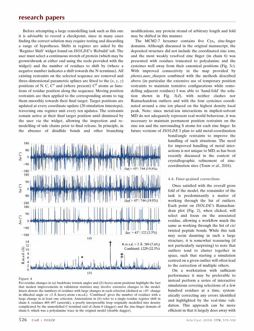
Figure 4Per-residue changes in (a) backbone torsion angles and (b) heavy-atom positions highlight the factthat modest improvements in validation statistics may involve extensive changes to the model.Insets denote the numbers of residues with large changes in each criterion (defined as >45� changein dihedral angle or >2 A heavy-atom r.m.s.d.). ‘Combined’ gives the number of residues with alarge change in at least one criterion. Annotations in (b) refer to a single-residue register shift inchain 4, residues 469–497 (asterisk), a poorly interpretable loop originally modelled into densitycomplicated by the unmodelled C-terminal end of chain 6 (dagger) and the zinc-finger domain ofchain 6, which was a polyalanine trace in the original model (double dagger).

the need to directly view the Ramachandran plot, and addi-

tionally reduces the overhead involved in repeatedly creating

and destroying simulations. To work through the 3ja8 model

once would require approximately 20–40 such simulations.

Once the number of Ramachandran outliers has been

reduced to the order of 0.1%, it is advisable to again equili-

brate the entire model against the map at some nonzero

temperature (the default is 100 K). It is common to see a

number of new outliers appear as formerly marginal residues

are pushed into disallowed conformations by their changed

surroundings. After two iterations of this approach, noting

that the proportion of residues in favoured Ramachandran

space remained below 90%, I saved the coordinates and [after

adding the missing ADP residues and the lysine described in

Fig. 3(b) using Coot] refined the model using phenix.real_

space_refine using its default settings (including the use of

Ramachandran and rotamer restraints). This improved the

proportion of favoured residues to 92% at the expense of a

slight increase in the number of outliers (0.43%) and the

introduction of a small number of twisted peptide bonds. After

re-equilibrating the result in ISOLDE I worked through the

remaining Ramachandran outliers as well as the lowest-

probability marginal residues. Re-equilibration at 100 K

followed by settling at 0 K left a single trans proline outlier on

the very edge of the �-helical region, which I was unable to

resolve in the ISOLDE environment. After running a final

round of phenix.real_space_refine without the use of Rama-

chandran restraints and using the input coordinates as a

reference model for backbone torsions, I obtained a final

result with the statistics described in Fig. 2(c), with an overall

MolProbity score of 1.44.

4.5. Analysis of changes

Looking only at the most commonly used overall validation

statistics, the nonspecialist reader may easily be led to the

conclusion that the changes made are quite modest. The

clashscore (defined as the number of steric clashes �0.4 A per

1000 atoms) has reduced from 32 to 2.35, the number of

Ramachandran outliers has reduced from 1.15% to zero and

the number of side-chain outliers has decreased from 0.1 to

0.03%. However, a more detailed residue-by-residue in-

spection (Fig. 4) reveals that obtaining a stable model with

these statistics required extensive changes throughout the

structure. Almost 20% of all ’ and dihedrals (and 3.5% of

all ! dihedrals) changed by more than 45�, while 7.6% of all

residues moved by more than 2 A on average. Overall, almost

a third of all residues in the model met at least one of the

above criteria. Perhaps most concerningly, re-refining the

deposited coordinates with the most recent available version

of phenix.real_space_refine with default parameters improved

the MolProbity score from 2.51 to 2.09 (most notably reducing

the clashscore to below 10), yet comparison of this with my

final structure yielded comparable results to those described

above.

research papers

Acta Cryst. (2018). D74, 519–530 Croll � ISOLDE 527

Figure 5Extensive rebuilding yields minimal changes in correlation to the map.Starting from the original model (blue), real-space refinement with thecurrent version of phenix.real_space_refine reduced the overall maskedFSC from 0.828 to 0.816, with some improvement in geometry. Rebuildingin ISOLDE followed by a tightly restrained phenix.real_space_refine runas described (black) increased the FSC to 0.821, while runningphenix.real_space_refine with default settings on the result (green)further increased the FSC to 0.830 with a slight degradation in geometry.These changes are far smaller than those arising from choice of mapsharpening or inclusion/exclusion of H atoms, for example. The verticaldotted line denotes the published resolution of the map.

Figure 6The relationship between model quality and fit to data breaks down indeposited 3.5–4 A resolution crystal (a) and cryo-EM (b) models. Thecrystal structure cohort was limited to models deposited from 2007 to thepresent, and Rfree values for data at �3.75 A and >3.75 A resolution areoffset by �0.0015 for clarity. All EM models in the resolution range withmasked CC � 0.5 were included in the analysis.

In light of the above, it is interesting to note that all changes

to the model described here yielded minimal changes to the

map–model Fourier shell correlation (FSC) as calculated using

phenix.model_vs_map (Fig. 5). This prompted me to perform a

brief analysis, comparing the MolProbity score with the fit to

data for all 3.5–4.0 A resolution crystal structures deposited in

the last decade and all 3.5–4.0 A resolution cryo-EM models

deposited to date (Fig. 6). All statistics other than EM model–

map correlation were gathered from the wwPDB validation

reports (Read et al., 2011); the latter were gathered from a

previous analysis (Afonine et al., 2018). The MolProbity score

was calculated from clashscore, rotamer outliers and

nonfavoured Ramachandran statistics as described previously

(Chen et al., 2010).

While it is indisputable that at high resolution model

geometric quality closely correlates with the fit to data, it is

clear that at these low resolutions this relationship has broken

down. This is perhaps not entirely surprising; after all, the fact

that many unphysical models may fit a low-resolution map is

the very reason restraints are necessary in the first place!

However, this does emphasize the ever-increasing need for

more restraints at low resolution, and in particular indicates

that the choice to accept a loss of geometric quality in return

for a slight gain in fit to the density is one that must be made

with great care.

5. Discussion

5.1. With great prestige comes great responsibility

Being the first to solve and publish the structure of an

important biological complex is a huge achievement which

rightly brings with it substantial prestige. The structure

discussed here is no exception: it is clearly the result of

extensive painstaking experimental and computational work,

deserving (in my opinion) of its publication in Nature.

However, when one is the first to publish a structure the

responsibility is greater than at any other time to ensure that

the structure is as correct as possible, since (at least until

substantially higher resolution data are collected) it is almost

certain to become the template upon which future studies of

the same complex are based. This case is no exception: since

the deposition of PDB entry 3ja8 in 2015 a further ten MCM-2

structures have been published by various authors, all of which

display a cohort of cis and twisted peptide bonds (mean 121,

minimum 87, maximum 140) which overlap substantially with

the original structure (Supplementary Fig. S4). As the pace of

structural biology depositions grows ever faster, this propa-

gation of errors through the database seems likely to become

more problematic.

5.2. Advantages and drawbacks of MD methods

The need for more and more prior information (in the form

of restraints) as the resolution of a data set decreases is a well

established truism in structural biology. In this context, MD

methods may be thought of as adding a very large yet difficult

to quantify set of additional restraints. Where traditional

model-building tools may consider only bonded interactions

and refinement tools aim to reduce nearest-neighbour atomic

clashes, in a typical MD simulation each individual atom ‘feels’

van der Waals and electrostatic force contributions from all

atoms within a 10 A radius: on the order of 1000 individual

pairwise forces for an atom in a well packed hydrophobic core.

Provided that the parameterization of these interactions is a

reasonable facsimile of reality, it is unsurprising that their

inclusion leads to improved results.

In particular, it can be argued that the clashscore is the most

sensitive of all of the standard conformational validation

metrics: whereas most Ramachandran and rotamer outliers

represent unusual strained conformations, a substantial

overlap of nonbonded atoms is a physical impossibility under

any conditions conducive to known life. Models with good

Ramachandran and rotamer statistics but poor clashscore

should therefore be treated with particular caution. I would

argue that this caution should extend to low-resolution models

with large numbers of missing side chains, since removing the

side chain gives the ability to achieve ‘allowed’ backbone

conformations that would cause severe clashes if the side-

chain atoms were present. The impossibility of clashes is

strictly reflected in the MD environment, with van der Waals

energy rising to infinity with 1/r12 for small interatomic

distances. Every step of an MD simulation therefore repre-

sents a structure with a clashscore very close to zero, which

combined with the strict inclusion of complete residues and

the explicit treatment of electrostatics leaves conformational

errors with fewer places to ‘hide’ compared with traditional

approaches.

A corollary to the above is that problems will arise where

classical MD parameterization is insufficient to replicate the

real-world behaviour of some chemical species. A well estab-

lished example is metal ions (Rode et al., 2005), where

substantial charge transfer (beyond the scope of classical MD)

often occurs between the ion and its neighbours. While

reasonable agreement with experiment is achievable with

careful parameterization in explicit solvent (Li, Song et al.,

2015), naive inclusion of these ions in an implicit solvent

environment leads to severe overestimation of long-range

electrostatic interactions, causing unmanageable distortion of

the surroundings. Given the many significant challenges facing

the use of explicit solvent in a model-building environment, it

appears prudent to carefully consider the best path forward

here. As a short-term (yet rather unsatisfying) measure, simply

artificially setting all metal-ion charges to +1.0 alleviates the

overestimation of long-range electrostatics while maintaining

reasonable van der Waals radii, allowing their use with the

careful application of suitable restraints with the aid of the

experimental map (as used here for handling the zinc-finger

domains). A near-term goal in ISOLDE is the addition of

automatically applied, user-adjustable distance and angle

restraints for metal centres. In the medium term, it may prove

valuable to develop a library of building blocks consisting of

metal–water clusters parameterized with varying levels of

completion of the first hydration shell. In the longer term, it

may be practical to provide an ab initio quantum-mechanical

research papers

528 Croll � ISOLDE Acta Cryst. (2018). D74, 519–530

treatment of these and other unusual sites, although it is likely

to be some time before single-workstation interactive perfor-

mance is possible.

It also must be noted that classical MD parameterizations

do not explicitly maintain the chirality of any given centre.

Rather, changes in chirality are blocked by energy barriers

that are effectively insurmountable under normal equilibrium

conditions. Chirality flips may occur under extreme conditions,

however; for example, in the vicinity of a complex multi-atom

clash in the starting model. While such events should be very

rare, I plan to add explicit chirality restraints in a future

version of ISOLDE. In the meantime, the chirality of all

centres in the final model should be checked with a tool such

as MolProbity.

6. Conclusions and future directions

For the purposes of this manuscript, I have demonstrated that

the ISOLDE environment combined with an existing refine-

ment package allows a single user, working on a moderately

priced workstation, to rebuild a large, low-resolution structure

to near-atomic resolution standards in approximately one

week of work, without reference to external information such

as reference models. This is not intended as a suggestion that

such extensive manual interaction is necessary or desirable. In

fact, it is likely that a majority of the improvements identified,

in particular those that involve simply flipping 1–2 adjacent

peptide bonds, should be readily manageable by automated

methods such as those recently described for use in moderate-

resolution crystal structures (Touw et al., 2015). In addition to

the many possible permutations in the use of ISOLDE with

external tools in a larger workflow, there is substantial scope

for the automation of various common tasks (and the imple-

mentation of existing successful algorithms) using combina-

tions of the various unit operations defined in ISOLDE itself.

A simple example of such a combination is the semi-

automated shifting of protein residues in register described in

x4.3, which is accomplished by the concerted action of many

moving position restraints.

Detailed inspection of the changes made to this model as

summarized in Fig. 4 presents some cause for concern, in

particular when contrasted against the minimal change in

correlation to the map (Fig. 5). While the number of outliers

by any standard validation metric changed by an apparently

modest amount (no more than 3.2% of residues/atoms) in

reality almost one third of all residues underwent a marked

change in backbone conformation and/or position. That the

conformation of the model can vary so substantially with such

modest changes in the resulting statistics strongly supports the

use of MD and similar environments, since these help to

exclude many configurations which are statistically ‘allowed’

but energetically unfavourable.

Acknowledgements

I thank Randy Read and Airlie McCoy (Cambridge) for their

many helpful discussions during the preparation of this

manuscript, and Tom Goddard (UCSF) for his extensive help

with the ChimeraX API.

Funding information

This work was supported by a Principal Research Fellowship

awarded to Randy J. Read by the Wellcome Trust (082961/Z/

07/Z).

References

Adams, P. D. et al. (2010). Acta Cryst. D66, 213–221.Afonine, P. V., Grosse-Kunstleve, R. W., Echols, N., Headd, J. J.,

Moriarty, N. W., Mustyakimov, M., Terwilliger, T. C., Urzhumtsev,A., Zwart, P. H. & Adams, P. D. (2012). Acta Cryst. D68, 352–367.

Afonine, P. V., Klaholz, B. P., Moriarty, N. W., Poon, B. K., Sobolev,O. V., Terwilliger, T. C., Adams, P. D. & Urzhumtsev, A. (2018).bioRxiv, https://doi.org/10.1101/279844.

Branden, C.-I. & Jones, T. A. (1990). Nature (London), 343, 687–689.

Brereton, A. E. & Karplus, P. A. (2016). Protein Sci. 25, 926–932.Brunger, A. T. (1992). X-PLOR Version 3.1. A System for X-ray

Crystallography and NMR. New Haven: Yale University Press.Chen, V. B., Arendall, W. B., Headd, J. J., Keedy, D. A., Immormino,

R. M., Kapral, G. J., Murray, L. W., Richardson, J. S. & Richardson,D. C. (2010). Acta Cryst. D66, 12–21.

Chen, V. B., Davis, I. W. & Richardson, D. C. (2009). Protein Sci. 18,2403–2409.

Conti, F., Barbagli, F., Balaniuk, R., Halg, M., Lu, C., Morris, D.,Sentis, L., Vileshin, E., Warren, J., Khatib, O. & Salisbury, K. (2003).EuroHaptics 2003: Proceedings, edited by I. Oakley, S. O’Modhrain& F. Newell, pp. 496–500. Dublin: Media Lab.

Cowtan, K. (2006). Acta Cryst. D62, 1002–1011.Croll, T. I. (2015). Acta Cryst. D71, 706–709.Croll, T. I. & Andersen, G. R. (2016). Acta Cryst. D72, 1006–

1016.Croll, T. I., Smith, B. J., Margetts, M. B., Whittaker, J., Weiss, M. A.,

Ward, C. W. & Lawrence, M. C. (2016). Structure, 24, 469–476.

Eastman, P., Swails, J., Chodera, J. D., McGibbon, R. T., Zhao, Y.,Beauchamp, K. A., Wang, L.-P., Simmonett, A. C., Harrigan, M. P.,Stern, C. D., Wiewiora, R. P., Brooks, B. R. & Pande, V. S. (2017).PLoS Comput. Biol. 13, e1005659.

Emsley, P. & Cowtan, K. (2004). Acta Cryst. D60, 2126–2132.Focht, D., Croll, T. I., Pedersen, B. P. & Nissen, P. (2017). Front.

Physiol. 8, 202.Goddard, T. D., Huang, C. C., Meng, E. C., Pettersen, E. F., Couch,

G. S., Morris, J. H. & Ferrin, T. E. (2017). Protein Sci. 27, 14–25.Hintze, B. J., Lewis, S. M., Richardson, J. S. & Richardson, D. C.

(2016). Proteins, 84, 1177–1189.Hooft, R. W. W., Vriend, G., Sander, C. & Abola, E. E. (1996). Nature

(London), 381, 272.Joosten, R. P., Joosten, K., Murshudov, G. N. & Perrakis, A. (2012).

Acta Cryst. D68, 484–496.Joosten, R. P., Long, F., Murshudov, G. N. & Perrakis, A. (2014).

IUCrJ, 1, 213–220.Joseph, A. P., Malhotra, S., Burnley, T., Wood, C., Clare, D. K., Winn,

M. & Topf, M. (2016). Methods, 100, 42–49.Kirmizialtin, S., Loerke, J., Behrmann, E., Spahn, C. M. T. &

Sanbonmatsu, K. Y. (2015). Methods Enzymol. 558, 497–514.Kleywegt, G. J. (2000). Acta Cryst. D56, 249–265.Kleywegt, G. J. & Jones, T. A. (1995). Structure, 3, 535–540.Langer, G., Cohen, S. X., Lamzin, V. S. & Perrakis, A. (2008). Nature

Protoc. 3, 1171–1179.Laskowski, R. A., MacArthur, M. W. & Thornton, J. M. (1998). Curr.

Opin. Struct. Biol. 8, 631–639.

research papers

Acta Cryst. (2018). D74, 519–530 Croll � ISOLDE 529

Li, P., Song, L. F. & Merz, K. M. Jr (2015). J. Phys. Chem. B, 119, 883–895.

Li, N., Zhai, Y., Zhang, Y., Li, W., Yang, M., Lei, J., Tye, B.-K. & Gao,N. (2015). Nature (London), 524, 186–191.

Maier, J. A., Martinez, C., Kasavajhala, K., Wickstrom, L., Hauser,K. E. & Simmerling, C. (2015). J. Chem. Theory Comput. 11, 3696–3713.

McNicholas, S., Croll, T., Burnley, T., Palmer, C. M., Hoh, S. W.,Jenkins, H. T., Dodson, E., Cowtan, K. & Agirre, J. (2017). ProteinSci. 27, 207–216.

McNicholas, S., Potterton, E., Wilson, K. S. & Noble, M. E. M. (2011).Acta Cryst. D67, 386–394.

Murshudov, G. N., Skubak, P., Lebedev, A. A., Pannu, N. S., Steiner,R. A., Nicholls, R. A., Winn, M. D., Long, F. & Vagin, A. A. (2011).Acta Cryst. D67, 355–367.

Nguyen, H., Roe, D. R. & Simmerling, C. (2013). J. Chem. TheoryComput. 9, 2020–2034.

Perez, A., MacCallum, J. L., Brini, E., Simmerling, C. & Dill,K. A. (2015). J. Chem. Theory Comput. 11, 4770–4779.

Read, R. J. et al. (2011). Structure, 19, 1395–1412.Rode, B. M., Schwenk, C. F., Hofer, T. S. & Randolf, B. R. (2005).

Coord. Chem. Rev. 249, 2993–3006.Stein, N. (2008). J. Appl. Cryst. 41, 641–643.Stewart, D. E., Sarkar, A. & Wampler, J. E. (1990). J. Mol. Biol. 214,

253–260.Terwilliger, T. C., Grosse-Kunstleve, R. W., Afonine, P. V., Moriarty,

N. W., Zwart, P. H., Hung, L.-W., Read, R. J. & Adams, P. D. (2008).Acta Cryst. D64, 61–69.

Touw, W. G., Joosten, R. P. & Vriend, G. (2015). Acta Cryst. D71,1604–1614.

Touw, W. G., van Beusekom, B., Evers, J. M. G., Vriend, G. & Joosten,R. P. (2016). Acta Cryst. D72, 1110–1118.

Trabuco, L. G., Villa, E., Mitra, K., Frank, J. & Schulten, K. (2008).Structure, 16, 673–683.

Wang, R. Y.-R., Song, Y., Barad, B. A., Cheng, Y., Fraser, J. S. &DiMaio, F. (2016). Elife, 5, e17219.

Winn, M. D. et al. (2011). Acta Cryst. D67, 235–242.Wlodawer, A., Minor, W., Dauter, Z. & Jaskolski, M. (2013). FEBS J.

280, 5705–5736.

research papers

530 Croll � ISOLDE Acta Cryst. (2018). D74, 519–530