j. stat. mech. - istituto nazionale di fisica nucleare

J. Stat. M

ech. (2015) P10010

Quasi equilibrium construction for the long time limit of glassy dynamics

Silvio Franz1, Giorgio Parisi2, Federico Ricci-Tersenghi2 and Pierfrancesco Urbani3

1 LPTMS, CNRS, Univ. Paris-Sud, Université Paris-Saclay, 91405 Orsay, France

2 Dipartimento di Fisica, INFN, Sezione di Roma I, and NANOTEC: CNR, Sapienza Universitá di Roma, P.le A. Moro 2, I-00185 Roma, Italy

3 Institut de physique théorique, Université Paris Saclay, CEA, CNRS, F-91191, Gif-sur-Yvette, France

E-mail: [email protected]

Received 15 June 2015Accepted for publication 20 August 2015 Published 9 October 2015

Online at stacks.iop.org/JSTAT/2015/P10010doi:10.1088/1742-5468/2015/10/P10010

Abstract. In this paper we review a recent proposal to understand the long time limit of glassy dynamics in terms of an appropriate Markov chain [1]. The advantages of the resulting construction are many. The first one is that it gives a quasi equilibrium description on how glassy systems explore the phase space in the slow relaxation part of their dynamics. The second one is that it gives an alternative way to obtain dynamical equations starting from a dynamical rule that is static in spirit. This provides a way to overcome the difficulties encountered in the short time part of the dynamics where current conservation must be enforced. We study this approach in detail in a prototypical mean field disordered spin system, namely the p-spin spherical model, showing how we can obtain the well known equations that describe its dynamics. Then we apply the same approach to structural glasses. We first derive a set of dynamical Ornstein-Zernike equations which are very general in nature. Finally we consider two possible closure schemes for them, namely the hypernetted chain approximation of liquid theory and a closure of the BBGKY hierarchy that has been recently introduced by Szamel. From both approaches we finally find a set of dynamical mode-coupling-like equations that are supposed to describe the system in the long time/slow dynamics regime.

Keywords: spin glasses (theory), slow dynamics and aging (theory), structural glasses (theory), slow relaxation and glassy dynamic

S Franz et al


Printed in the UK

P10010

JSMTC6

© 2015 IOP Publishing Ltd and SISSA Medialab srl

2015

15

J. Stat. Mech.

JSTAT

1742-5468

10.1088/1742-5468/2015/10/P10010

PAPERS

10

Journal of Statistical Mechanics: Theory and Experiment

© 2015 IOP Publishing Ltd and SISSA Medialab srl

ournal of Statistical Mechanics:J Theory and Experiment

IOP

1742-5468/15/P10010+19$33.00


2doi:10.1088/1742-5468/2015/10/P10010

J. Stat. M

ech. (2015) P10010

I. Introduction

Glass is an out of equilibrium state of matter. Left by themselves, the microscopic configurations and macroscopic properties of glass slowly change in a process known as physical aging, where the free-energy evolves towards lower and lower values. This process is very slow and is characterized by a separation of time scales, where fast degrees of freedom appear to be in thermal equilibrium in the background of the slow degrees of freedom. The evolution of the latter is sometimes described as an effective random walk in configuration space, depicted as a rough free-energy landscape, where the system wanders from one metastable state to another. The rules by which the metastable states are selected in the dynamical process determine the observed proper-ties of the systems. A leading role in the comprehension of slow off-equilibrium dynam-ics of glassy systems is played by mean field theory (see [2] for a review), which allows asymptotic aging regimes to be described through scaling laws and effective tempera-tures associated with the violations of the fluctuation dissipation theorem [3, 4]. The analysis performed in [5, 6] and in [7–11] related these effective temperatures to the quasi-equilibrium selection of metastable states during glassy dynamics. This notion of quasi-equilibrium exploration can be formalized through the introduction of a suit-able Markov chain where fast times are effectively coarse grained, and it is assumed the set of states available at any give time, which are the ones at a specific distance

Contents

I. Introduction 2

II. The Boltzmann pseudodynamics construction 3II.A. Response functions . . . . . . . . . . . . . . . . . . . . . . . . . . . . . . . . . . 4II.B. Equilibrium measure . . . . . . . . . . . . . . . . . . . . . . . . . . . . . . . . . 6

III. Mean-field glassy dynamics 7III.A. The long chain limit . . . . . . . . . . . . . . . . . . . . . . . . . . . . . . . . 9

IV. Replicas 10

V. Boltzmann pseudodynamics for supercooled liquids 13V.A. Closure schemes . . . . . . . . . . . . . . . . . . . . . . . . . . . . . . . . . . . 15

V.A.1. Dynamical HNC equation . . . . . . . . . . . . . . . . . . . . . . . . . 15V.A.2. MCT from BPDe . . . . . . . . . . . . . . . . . . . . . . . . . . . . . . 18

VI. Conclusions 18

Acknowledgments 19

References 19


3doi:10.1088/1742-5468/2015/10/P10010

J. Stat. M

ech. (2015) P10010

from the present state, are selected by a Boltzmann law [1]. This chain construction reproduces the results of long time relaxational dynamics within mean-field theory and it gives the correct long time dynamical equations whenever the system has a finite configurational entropy. We believe that it captures the principles of the explora-tion of configuration space in glasses also in realistic systems where metastable states are sufficiently long-lived. Moreover, since the short timescales are completely coarse grained, the method automatically produces time reparametrization invariant equa-tions. Thanks to the Boltzmann prescription, the chain shares many formal features with equilibrium systems. This observation straightforwardly suggests simple ways to treat long time dynamics of structural glassy systems taking advantage of standard approximation schemes originally devised to study equilibrium [12]. Moreover, since short times are coarse-grained, constraints such as energy and mass conservation that complicate short time analysis are not relevant here. In this contribution we review the main results of our approach and present some new results and derivations that were just hinted at in previous publications. The paper is organized as follows: in the first section we introduce the basic dynamical construction and we discuss the response properties of the system and its equilibrium measure. In the second section we discuss spin glass mean field theory, and we give a new derivation of the dynamical equa-tions through a probabilistic analysis. This avoids the use of replicas which were used in a previous publication [1]. Then we present the results of the direct integration of our equations that have never been published before. In the third section we review the applications to realistic liquid models. We present the derivation of a dynamical ver-sion of the Ornstein-Zernike equation. We complement this equation with two closure schemes that give both a final dynamical equation that is of the same kind of standard mode-coupling theory (MCT). Within this scheme we are able to predict the properties of the dynamics both in the equilibrium regime and in the aging one.

II. The Boltzmann pseudodynamics construction

In this section we review the Boltzmann pseudodynamics (BPD) construction recently introduced in [1] and we show some generalities about correlation and response functions that can be computed using this formalism. Let us consider a system described by a set of internal degrees of freedom that we call Si and that will be addressed as spin variables (our notation is very close to the one encountered in spin systems but can also be used to treat particles in a liquid where the internal degrees of freedom are the position of the particles). In the following we will define a dynamical rule to evolve such a system so that we will indicate with Si(t) the configuration of the system at time t. The BPD is a discrete time dynamics defined from the following dynamical rule: given the configuration of the spins at time t, the configuration at time t + 1 occur with a probability that is given by

( ( ) ( ))[ ( )]

( ( ) ( ( ) ( )))

[ ( )] ( ( ) ( ( ) ( )))

[ ( )]

( )

[ ( )]∑β

δ

β δ

_ + |_ =_

_ + − _ _ +

_ = _ + − _ _ +

∼

∼

β

β

+

− +

+_ +

− +

+

+

M S t S tZ S t

C t t q S t S t

Z S t C t t q S t S t

11

;e , 1 , 1

; e , 1 , 1

t

H S t

tS t

H S t

1

1

11

1

t

t

1

1

(1)


4doi:10.1088/1742-5468/2015/10/P10010

J. Stat. M

ech. (2015) P10010

The function ( )σ τq , is an overlap function that measures the similarity between the configurations σ and τ. For the spin system it is given simply by ( )σ τ στ= ∑q N, /i i i where σi and τi are the values of the spin in the two configurations. For particle systems instead one can choose between many different definitions. A simple possibility is to use the same function as for spin systems through a lattice gas coding of the liquid configurations, e.g. by dividing the volume in small cells and defining binary variables that code for occupation numbers of the cells4. The probability of a trajectory given an

initial configuration ( )_S 0 at time t = 0 is given by

[ ( ) ( ) ( ) ( )] ˆ[ ( )] ( ( ) ( ))∏_ _ − … _ |_ = _ _ + |_=

−P S t S t S S P S M S k S k, 1 , , 1 0 0 1

k

t

1

1

(3)

where P̂ is a given measure over the inital conditions. Note that in the above dynamics

we fix the set of variables { ( )}+∼C t t1, and { }βt from the outside. In glassy dynamics

the temperatures are naturally fixed to the value of the thermal bath, while ( )+∼C t t1,

should be chosen in a self-consistent way in order to achieve the right separation between fast and slow time scales. While in certain applications it can be interesting to consider a time dependence of the temperature, from now on in this paper we will consider the case of β constant in time. We will show in the following that this pseu-dodynamics provides a coarse grained description of real time dynamics in which fast

processes are seen as instantaneous. For finite values of the choosen values ( )+∼C t t1, ,

at each time step then the system chooses a configuration at a macroscopic distance from the previous one. This configuration is chosen as an equilbrium one at the pre-scribed distance. In this sense the ‘fast’ time scales that in real dynamics are needed to equilibrate within a metastable state are coarse-grained. The main assumption is

that all configurations satisfying the constraint =∼

q C are equally reachable by the fast relaxation processes. This assumption is fine if

∼C is properly chosen, e.g. a value close

to the typical overlap qEA.A computer implementation of (1) would require for each step of the chain a Monte

Carlo simulation in which the fast time scale is reinserted to achieve the prescribed sampling. For that reason we call it pseudodynamics. We will be interested in the long chain limit in which the relevant time scales are much larger than the unit of the elementary time step and the system moves to even larger distances than the ones reached in a single step.

II.A. Response functions

A fundamental characterization of a glassy dynamics is provided by the linear response functions. Their relation with fluctuations during aging shows, both in mean-field

4 Another popular choice in systems of particles is to use

( ) ( )∑= | − |q X YN

w x y,1

i ji j

,

(2)

where { }=X x x, ..., n1 and { }=Y y y, ..., N1 , are two configurations of N particles and where w is some positive short

ranged function, e.g. ( ) ( )σ= −w r rexp /2 2 .


5doi:10.1088/1742-5468/2015/10/P10010

J. Stat. M

ech. (2015) P10010

theory [3, 13] and in simulations [14] the emergence of effective temperatures ruling the exchanges of energy between slow degrees of freedom. It has been proposed in [15] that non trivial response and effective temperatures in non-equilibrium dynamics are pos-sible if trajectories (clones) starting in the same point and subject to different thermal noise get separated during their evolution. One can define the clone correlation function

of a simple observable as for example the magnetization ( ( ))_m S t as follows

( ) [ ( ( ) ( )) ( ( ) ( ))]( )E E E ≡ _ |_ |_ >Q t u m t S s m u S s t u s, for , .s S s

The internal expectations denoted by ( )E ⋅ are the averages over independent thermal

trajectories that start from the same initial configuration ( )_S s at time s, while ( )E_S s is the average over these initial configurations. In [15] the conjecture was put for-ward that non trivial effective temperatures are only possible for systems where large time separation Qs(t, u) tends to the same minimal value as the correlation C(t, u) itself. This is different from systems undergoing domain coarsening in phase separation where Q remains much larger then C and a non trivial response in the aging regime is absent. Unfortunately, despite empirical evidence, a formal relation between response and clone correlation function was lacking. In the dynamics we just introduced this relation emerges naturally for pseudo-times u = s + 1 and t > u corresponding to real times ≫t u and s, u such that C(u, s) is in the beta relaxation regime. Consider the

dynamics (1) in a time dependent field ht coupled with an observable ( ( ))_m S t , function

of the system configuration ( )_S t . The Hamiltonian in the presence of the field is

( ( )) ( ( )) ( ( ))_ = _ − _H S t H S t h m S t .h t (4)

The response function is defined as usual

( )⟨ ( ( ))⟩

∆ =∂ _

∂t s

m S t

h,

s (5)

where the average is done over the multiple realizations of the trajectories of the sys-tem. Because of the causal structure of the Markov chain (1), the response function is non zero only if t > s. To analyse this quantity we start from

hP S t S t S S m S s

m S s S s P S t S t S S

, 1 , ..., 1 0

1 , 1 , ..., 1 0

s( ( ) ( ) ( ) ( )) ( ( ( ))

[ ( ( )) ( )]) ( ( ) ( ) ( ) ( ))

β∂∂

− | =

− | − − |E

(6)

where

[ ( ( )) ( )][ ( )]

( ) ( ( ( )) ( ))( )E ∑βδ_ |_ − =

_ −_ _ _ _ − − −

∼′ ′β−

′

′m S s S sZ S s

m S q S S s C s s11

; 1e , 1 , 1 .

S

H S

(7)This leads to

(( ) [⟨ ( ( )) ( ( ))⟩ ⟨ ( ( )) [ ( ( )) ))⟩] [ ( ) ( )]β β∆ = − | − = −Et s m S t m S s m S t m S s S s C t s D t s, 1 , , (8)

where


6doi:10.1088/1742-5468/2015/10/P10010

J. Stat. M

ech. (2015) P10010

⟨ ( ( ))⟩ ( ( )) ( ( ) ( ) ( ) ( )) ˆ( ( ))

( ) ⟨ ( ( )) ( ( ))⟩ ( ) ⟨ ( ) ( ( ( )) ( ))⟩ ( )( ) ( )

∑ ∑= … − |

= = | − =′ −

A S s A S s P S t S t S S P S

C t s m S t m S s D t s m t E m S s S s Q t s

, 1 , ..., 1 0 0 ,

, , , 1 , .S t S

s

0

1

(9)

Notice that, by simple properties of conditional probability, if t < s one has D(t, s) = C(t, s) and the response is ( )∆ =t s, 0 as it should be. Equation (9) provides the announced relation between response and clone correlation: a response at large times is only pos-sible if Qs−1(t, s) = D(t, s) differs from C(t, s).

We would like now to make some remarks on the long chain (i.e. long time) limit. By

properly choosing the constraining value close to the typical overlap value, ≈∼C qEA, all the

fast dynamics are coarse-grained in a single step of the pseudodynamics. Consequently, we have ( ) ≈C t t q, EA and the equal time response ( ) [⟨ ( ) ⟩ ⟨ ( )⟩ ]β∆ = −t t m t m t, 2 2 , corre-sponding to the equilibrium-like response in the beta regime, is expected to be a quan-tity of order one, which coincides with [ ( ) ( )]β − +C t t C t t, 1, since D(t, t) should be close to C(t + 1, t). On the other hand if t > s (to be intended as ≫t s in real times) one can expect D(t, s) to be close to C(t, s). For a chain of length t the total susceptibility to a field that acts from time 1 to t, is ( ) ( )χ = ∑ ∆=t t s,s

t1 . This quantity remains finite

for → ∞t if ( ) ( )∆ =t s R t s s, , d is infinitesimal in the continuous time limit. In this way the sum converges to

( ) ( ) ( )∫χ = ∆ +t t t s R t s, d , ,t

0 (10)

where the first and second terms are respectively the responses from the fast and the slow dynamics. A non trivial response in the long time regime is thus associated with a non zero response function R(t, s), i.e. to decaying clone correlation function that in the continuum limit is ( ) ( ) ( )+ = −Q t s ds C t s s T R t s, , d ,s , since in the fast dynamics the fluctuation-dissipation relation ( ) ( )∂ =C t s T R t s, ,s holds.

II.B. Equilibrium measure

Despite the fact that we are interested in the applications of (1) to glassy dynamics and time scales where equilibration does not occur, in general, for time independent correla-

tions ( )+ =∼ ∼C s s C1, and finite system’s volumes, the Markov chain (1) is ergodic and

it is interesting to study its equilibrium measure. This is not the ordinary Boltzmann distribution. In fact we can observe that the detailed balance is verified with respect to the modified distribution

( ) ( )( )µ β= _ _β−SZ

Z S1

e ,H S

2 (11)

where

( ( ) )[ ( ) ( )]∑ δ= _ _ _ _ −∼

′β

_ _

− +

′

′Z q S S Ce ,S S

H S H S2

, (12)


7doi:10.1088/1742-5468/2015/10/P10010

J. Stat. M

ech. (2015) P10010

This is therefore the equilibrium distribution of the chain. Equivalently one can see that the measure for two configurations at consecutive times is

( ) ( ( ) )[ ( ) ( )]µ δ= −∼

′ ′β− + ′S SZ

q S S C,1

e , .H S H S2

2 (13)

III. Mean-field glassy dynamics

In this section we would like to analyse mean field spin glasses and show how to obtain a full characterization of the dynamics in terms of a single correlation function and its conjugated response function. The analysis was previously performed in [1] with the aid of a replica method that can be employed to treat analytically the denominators in (1). Here we propose an alternative derivation that avoids the use of replicas similar to the derivation of mean-field dynamical equations for Langevin dynamics presented in [16].

We consider specifically the spherical p-spin model which provides the canonical example of mean-field glassy dynamics. The Hamiltonian of the model is

[ ] [ ]∑ ∑ ∑= − … − = ∝ −<…<

…= =

…

−

…

⎡⎣⎢

⎤⎦⎥H S h J S S h S S N P J

N

pJ; exp

!J

i ii i i i

i

N

i ii

N

i i i

p

i i, ,1 1

21

2

p

p p p p

1

1 1 1 1

(14)where we have introduced a site dependent magnetic field in the system that is needed in order to compute the response function. In order to make the presentation as simple as possible we will restrict our analysis to the case p = 3 even if the general case is a straightforward generalization of this one.

Due to the mean field nature of the model, we can get closed dynamical equations in terms of two point correlation and response functions. Let us consider an arbitrary

function or operator ( )φ S dependent on a trajectory { ( )}= _ τ=

S uSu 0

and write the obvi-ous identity

S sP SS S Sd 0 0J

i( )[ ( ) ( ( ))]∫ φ∂

∂| =E (15)

where, EJ represents the average over the disordered couplings. In order to obtain equations for correlation and response functions it is enough to consider the insertion

of ( ) ( )φ τ=S Si and ( ) ( )φ = δδ τ

Shi

, which do not depend on the quenched variables J, we

can therefore average direcly the measure ( ( ))|_P SS 0

SP S J S S S

S S S P S

S

S S

01

2

1 1 1 0

.

Ji

Jj k

ijk j k i

i i i

,

1 }( )

( ( )) ( ) ( ) ( )

( ) [ ( ) ( ( ) ( ))] ( ( ))

E E

E

∑σβ σ σ µ σ

ν σ ν σ σ σ

∂∂

| = +

+ − + + − + | |

σ

σ σ+

⎪

⎪⎧⎨⎩

⎡⎣⎢⎢

⎤⎦⎥

(16)


8doi:10.1088/1742-5468/2015/10/P10010

J. Stat. M

ech. (2015) P10010

In order to simplify our analysis we suppose that ( )_S 0 is chosen randomly with uni-form probability on the sphere and ( ( ))_P S 0 is independent of J. In the case where

( ( ))_P S 0 depends of J additional terms would appear (see e.g. [16]). We can now integrate by part the Jijk in the first term of (16) which results in the substitution

J S S S S S S S 1ijk N i j k i j k3

2 β→ ∑ − −ε ε ε ε ε ε εε E[ ( ) ( ) ( ) ( ( ) ( ) ( )| ( ))] to get

}( )

( ( )) [ ( ) ( ) ( )

( ( ) ( ) ( ) ( ))] ( ) ( ) ( ) ( )

[ ( ) ( ( ) ( ))] ( ( ))

E E

E

E

ε ε ε

ε ε ε ε

ε∑ ∑σβ β

σ σ µ σ ν σ

ν σ σ σ

∂∂

| =

− | − + + −

+ + − + | |

σ σ

σ+

⎪

⎪⎧⎨⎩

⎡⎣⎢⎢

⎤⎦⎥

SP S

NS S S

S S S S S S S

S S P S

S

S

S S

03

2

1 1

1 1 0 .

Ji

Jj k

i j k

i j k j k i i

i i

2,

1

(17)

We will make at this point the crucial hypothesis that for typical trajectories

( ) ( )τ σ∑ S SN j i i1 and S S S 1

N i i i1 ( ) ( ( ) ( ))Eτ σ σ∑ | − are self-averaging quantities and coin-

cide respectively with ( )τ σC , and ( )τ σD , . This hypothesis is equivalent to the factor-ization, for ≠i j, ⟨ ( ) ( ) ( ) ( )⟩ ⟨ ( ) ( )⟩⟨ ( ) ( )⟩τ σ τ σ τ σ τ σ=S S S S S S S Si i j j i i j j and analogous formulas for more then two indices. The ‘clustering conditions’ of the correlation functions, which imply that the averages are dominated by a single pure state, exclude a priori replica symmetry breaking (RSB) effects. It is of course possible to include RSB effects even if in the long chain limit the RSB effects are indistinguishable from violations of fluctuation dissipation theorem (FDT) within the RS formalism. Using the factoriza-tion hypothesis we finally get

⎧⎨⎩⎡⎣⎢S

P S S C S D

S S S

S P S

S S

S S

03

2, 1 ,

1 1

1 0 .

Ji

J i i

i i i

i

2 2

1

}]

( )( ( )) [ ( ) ( ) ( ( ) ( )) ( ) ]

( ) ( ) [ ( )( ( ) ( ))] ( ( ))

∑σ

β β σ σ

µ σ ν σ ν σ

σ σ

∂∂

| = − | −

+ + − + +

− + | |σ σ σ+

ε ε ε ε εε

E E E

E

(18)

Inserting at this point ( ) ( )φ τ=S Si and ( ) ( )φ = δδ τ

Shi

and performing the sum over the

trajectories we get respectively:

( ) [ ( ) ( ) ( ) ( ) ]

( ) ( ) ( )

∑δ τ σ β τ σ τ σ

µ τ σ ν τ σ ν τ σ

− − = −

+ + − + ∆ +

τ

σ σ σ

=

+

ε ε ε εε

C C D D

C C

, , , ,

, , 1 , 1 ,

0

2 2

1

(19)

C D0 , , , ,

, 1 1, 1 .

2 2

, 1 1

( ) [ ( ) ( ) ] ( )

( ) ( )

∑ β τ σ σ µ τ σ

ν τ σ δ ν σ σ

= ∆ − + ∆

+ ∆ − + ∆ + +

τ

σ

σ

σ τ σ σ

=

+ +

ε ε εε

(20)

These equations have a causal structure that is inherited from the chain construc-tion and can be integrated iteratively step by step. In the next section we show that


9doi:10.1088/1742-5468/2015/10/P10010

J. Stat. M

ech. (2015) P10010

assuming the existence of a long chain limit, these equations reduce to the long time equations for the slow part of the Langevin dynamics of the same model. The consis-tency of this limit can be checked through explicit integration of the equations. At low

temperatures, one finds an aging regime where self-consistently ( ) →τ τ+∼C q, 1 EA while

→ντ 0 at large τ.

III.A. The long chain limit

The equations (19) and (20) can be easily generalized to arbitrary spherical long range

spin glass models with a Hamiltonian of p-spin mixture type [ ] [ ]_ = ∑ _H S a H Sp p p and

correlation function ( ( ) ( )) ( )= ⋅′ ′E H S H S Nf S S N/ , with ( ) = ∑f q a qp pp1

22 . It is inter-

esting to write them in the general case:

C f C D f D C

C

, , , , ,

, 1 , 1

0

1

( ) [ ( ) ( ( ) ( ) ( ( ))] ( )

( ) ( )

∑δ τ σ β τ σ τ σ µ τ σ

ν τ σ ν τ σ

− − = − +

+ − + ∆ +

′ ′τ

σ

σ σ

=

+

ε ε ε εε

(21)

f C f D0 , , , ,

, 1 1, 1 ., 1 1

( ) [ ( ( )) ( ( ))] ( )

( ) ( )

∑ β τ σ σ µ τ σ

ν τ σ δ ν σ σ

= ∆ − + ∆

+ ∆ − + ∆ + +

′ ′τ

σ

σ

σ τ σ σ

=

+ +

ε ε εε

(22)

In the continuum time limit, using ( ) ( ) ( )= −D t s C t s T R t s s, , , d for t > s, and fixing

ν = 0t , that corresponds to using the saddle-point value qEA for ( )−∼C t t, 1 , we get

( ) ( ) ( ( )) ( ) ( ( )) ( ) ( )

( ( ) ( )) ( ) ( ( ))( )

( ) ( ) ( ( )) ( ) ( )

( ( )) ( )( ) ( ( ) ( )) ( )( ) ( ( ) ( ))

( ( ( )) ( ) ( ( )) ( ) ( ))

∫ ∫

∫

∫

″

″

″

″

µ β β

β β

µ β

β βµ β

β

= +

+ − + −

=

+ − + −= + −

+ +

′

′ ′ ′

′ ′′ ′

′

t C t u s f C t s R u s s f C t s R t s C u s

f f q C t u f C t u q

t R t u sf C t s R t s R s u

f C t u R t u q f f q R t u

t T f f q

s f C t s R t s f C t s R t s C t s

, d , , d , , ,

1 , , 1

, d , , ,

, , 1 1 , ,

1

d , , , , ,

u t

EA EA

u

t

EA EA

EAt

0 02 2

2

0

(23)

where we used the condition ( ) =∼C t t, 1 and C(t, t) = qEA. These are well known equa-

tions that in the dynamic theory of mean field spin glasses, depending on the mod-els, have a dynamical phase transition below which there are aging solutions where fluctuation dissipation theorem and time translation invariance do not hold.

In order to check the consistency of the aging solutions and the long time limit of the original Markov chain, we have integrated explicitly the discrete BPD equa-

tions for the pure p-spin model for p = 3 with ( ) =f q q1

23 and for a mixture of p = 2

and p = 4 with ( ) = +f q q q1

22 1

204. It is interesting to consider both models since, as

is well known, the former has a one-step replica symmetry breaking (1RSB) phase


10doi:10.1088/1742-5468/2015/10/P10010

J. Stat. M

ech. (2015) P10010

and displays aging with a single (inverse) effective temperature [3] β β= Xeff while the latter has a full replica symmetry breaking (fRSB) phase and has a continuum set of effective temperatures q X q f q f q/eff

3/2( ) ( ) ( ) ( )″′ ″β β= = that during aging depend continuously on the value of the correlation function C(t, u) = q. We integrated the

equations in the low temperature regime with ( )−∼C t t, 1 fixed to the theoretical value

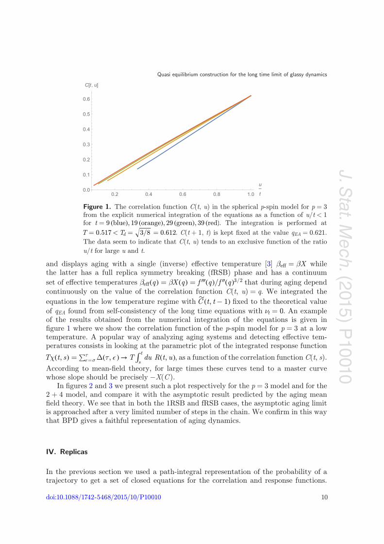
of qEA found from self-consistency of the long time equations with ν = 0t . An example of the results obtained from the numerical integration of the equations is given in figure 1 where we show the correlation function of the p-spin model for p = 3 at a low temperature. A popular way of analyzing aging systems and detecting effective tem-peratures consists in looking at the parametric plot of the integrated response function

( ) ( ) → ( )εε ∫χ τ= ∑ ∆στ=T t s T du R t u, , ,

s

t, as a function of the correlation function C(t, s).

According to mean-field theory, for large times these curves tend to a master curve whose slope should be precisely −X(C ).

In figures 2 and 3 we present such a plot respectively for the p = 3 model and for the 2 + 4 model, and compare it with the asymptotic result predicted by the aging mean field theory. We see that in both the 1RSB and fRSB cases, the asymptotic aging limit is approached after a very limited number of steps in the chain. We confirm in this way that BPD gives a faithful representation of aging dynamics.

IV. Replicas

In the previous section we used a path-integral representation of the probability of a trajectory to get a set of closed equations for the correlation and response functions.

Figure 1. The correlation function C(t, u) in the spherical p-spin model for p = 3 from the explicit numerical integration of the equations as a function of u/t < 1 for ( ) ( ) ( ) ( )=t 9 blue , 19 orange , 29 green , 39 red . The integration is performed at

= < = =T T0.517 3/8 0.612d . C(t + 1, t) is kept fixed at the value qEA = 0.621.

The data seem to indicate that C(t, u) tends to an exclusive function of the ratio

u/t for large u and t.


11doi:10.1088/1742-5468/2015/10/P10010

J. Stat. M

ech. (2015) P10010

In the case of systems with long range interactions an alternative way to produce the dynamical equations is by treating the denominators that appear in the definition (1) of the Boltzmann-Markov chain with the replica method. This consists of substituting all the theoretical computations of the denominator appearing in (1) by a positive power of the constrained partition function to get

Figure 2. The plot of rescaled susceptibility ( )χT t u, as a function of C(t, u) in the p-spin model for p = 3. The lines are computed at times t 9 blue , 19 orange , 29 green , 39 red( ) ( ) ( ) ( )= and the temperature is T = 0.517

( = =T 3/8 0.612d ). We also plot the FDT line 1 − C and the modified FD

prediction ( )− + −q X q C1 EA EA . The value of the fluctuation-dissipation ratio predicted by the long time dynamics of the Langevin equation is X = 0.610 and coincides well with the data.

Figure 3. The plot of the rescaled susceptibility ( )χT t u, as a function of C(t, u) for

( ) ( ) ( )=t 10 blue , 20 orange , 30 green in the 2 + 4 model with ( ) ( )= +f q q aq1

22 4 and

a = 0.1 at temperature T = 0.34. The critical temperature of the model is =T 1c . We also plot the FDT line 1 − C and the modified FD prediction from RSB, which show the good agreement of the BPD with the expected results for infinite time prediction.


12doi:10.1088/1742-5468/2015/10/P10010

J. Stat. M

ech. (2015) P10010

( ( ) ( )) [ ( )] ( ( ) ( ( ) ( )))[ ( )]β δ_ + |_ = _ _ + − _ _ +∼β− − +

++M S t S t Z S t C t t q S t S t1 ; e , 1 , 1n

n H S t1 1t

t1

1

(24)

The new chain depends on the parameters nt+1 that for each time t counts the ‘num-ber of replicas’. As usual in the replica method, these numbers are considered integers in intermediate computations, but set to zero in the replica limit where (24) coincides with (1). Renaming the ‘master replica’ S(t) = S0(t) and introducing nt − 1 ‘slave rep-licas’ Sa(t), a = 1, ..., nt − 1, we get:

M S t S t C t t q S t S t1 e , 1 , 1n

S t

H S t

a

na0 0

1

1

0

10

t

aa

nt

a

nt at

1

11 1

01 1 1

( ( ) ( )) ( ( ) ( ( ) ( ))){ ( )}

[ ( )]∑ ∏ δ+ | = + − +∼∑β

+

− +

=

−

+

=+ −

=+ − +

(25)

The dynamical equations for the correlations and response functions in the case of the p-spin spherical model (24) were first derived with this formalism in [1]. Within the replica method it is natural to introduce the total partition function up to time t

( ) ( ( ( ) ( )) ( ))( )

[ ]∑ ∏ δ= − − −∑β−Z t q S u S u C u ue , 1 , 1S u

H S

u a

atot

,

0

a

u a ta

,

(26)

where in the sum and the product u runs up to t and, for each u, a runs from 0 to nu − 1. This expression, complicated as it may be, has the same formal structure of a partition function of a replicated equilibrium system. The difference with the usual case is that here we have an explicit interaction between replicas at subsequent times due to the chain constraint. As in the usual case however, the finite nt system can be interpreted as a mixture of interacting particles of different kinds. In this way this is a good starting point for approximations. Indeed one can apply quite straightforwardly all existing approximations for equilibrium mixtures modulo parametrizations of the quantities of interest that allow for the analytic continuation needed to take the replica limit. As usual, considerations of symmetry under permutations of different replicas play an important role. In the present case, different from the equilibrium case where all replicas are equivalent, the partition function (26) is only invariant under independent permutations of groups of slave replicas with the same time index.

In replica calculations it is quite simple to see that a prominent role in manipulating (26) is played by the replica correlation function ( ) ⟨ ( ) ( )⟩=Q s u S s S u,ab

a b . This codes for both the correlation and the response functions of the previous section. Assuming rep-lica symmetry (i.e. invariance under the previously mentioned group of permutations), we can write the most generic replica symmetric parametrization for the overlap matrix

( ) ( ) ( ) ( ) ( )δ δ δ δ= + ∆ + ∆ + ∆Q s u C s u s u u s u u, , , , , .ab b a s u a b,1 ,1 , , (27)

In the long chain continuous time limit this becomes:

( ) ( ) ( ) ( ) ( ) ( ) [ ( ) ( )]θ δ θ δ δ δ= + − + − + −∼

Q s u C s u R s u u s u R u s s s u C u u C u u, , , d , d , , .ab b a s u a b,1 ,1 , ,

(28)

In [1] it has been shown that this parametrization reproduces the correct dynamical equations for this model in the slow dynamical regime. In the next section we will deeply use this form in the context of the replicated liquid theory in order to obtain a set of new dynamical equations for structural glasses [12].


13doi:10.1088/1742-5468/2015/10/P10010

J. Stat. M

ech. (2015) P10010

V. Boltzmann pseudodynamics for supercooled liquids

In this section we want to develop the BPD formalism to describe the slow regime of the dynamics of supercooled liquids undergoing a glass transition. As we emphasized in the previous section this can be done quite easily. Indeed the BPD construction can be directly applied to the replicated liquid theory that has been successfully employed to describe the glass transition [17–22]. In particular we can take the equations of the replicated liquid theory used to obtain the statics of structural glasses and plug the pseudodynamics ansatz inside them. Practically, in doing this we have to promote simple replica indices to BPD replica indices → ( )α t a, .

Let us see how all this procedure works. We start from the definition of the basic quan-tities that can be treated in the theory of the replicated liquid [18]. The simplest objects we need are the density field and its two point correlation function that are defined by

( ) ⟨ ( )⟩ ( ) ⟨ ( ) ( )⟩( )

[ ]

( ) ( )∑ ∑ρ δ ρ δ δ= − = − −αα

αβα β

=x x x x y x x y x;

i

N

iij

i j1

(29)

where the sum over [ij] runs on all i, j if α β≠ and over ≠i j if α β= . Moreover we define

( )( )

( ) ( )ρρ ρ

= −αβαβ

α βh x y

x y

x y,

,1 ; (30)

in what follows we will always look for a uniform solution for the density field such that ( )ρ ρ=α x .

We introduce also the direct correlation function ( )αβc x that is defined by the repli-cated Orstein-Zernike (OZ) equation:

( ) ( ) ( ) ( )∫∑ ρ= − −αβ αβγ

αγ βγ=

c x h x y h x y c yd .n

1

tot

(31)

It is convenient also to rewrite the same equations in Fourier space

( ) ( ) ( ) ( )∑ ρ= −αβ αβγ

αγ βγ=

c q h q h q c q .n

1

tot

(32)

In the glass phase and within a 1RSB picture, the static version of the OZ equation can be written as

˜( ) ˜( ) [ ˜( ) ˜( ) ( ) ( ) ( )]ρ= + + −h q c q h q c q m h q c q1 (33)

( ) ( ) [ ˜( ) ( ) ˜( ) ( ) ( ) ( ) ( )]ρ= + + + −h q c q h q c q c q h q m h q c q2 (34)

where m is the number of replicas. In the limit →m 1 we get the OZ equations that are needed to compute the dynamical MCT transition point

˜( ) ˜( ) ˜( ) ˜( )ρ= +h q c q h q c q (35)

( ) ( ) [ ˜( ) ( ) ˜( ) ( ) ( ) ( )]ρ= + + −h q c q h q c q c q h q h q c q (36)


14doi:10.1088/1742-5468/2015/10/P10010

J. Stat. M

ech. (2015) P10010

where c̃ and c are respectively the diagonal and off-diagonal parts of the matrix αβc and the same is true for αβh . These quantities can be thought of as the corresponding cor-relation functions for the supercooled liquid for times that are such that any dynami-cal correlation function is close to its plateau value. In particular they can be used to compute the MCT non ergodicity parameter.

We want to show that once the relevant generalization of (28) is considered for αβc and αβh , the equation (32) has formally the structure of a long time mode-coupling equation which can be used both to describe equilibrium slowing down as the glass transition is approached and the aging dynamics below the glass transition point.

As in the simple case of (28) where there is no space dependence, the replica depen-dence of h and c encode for correlation and response functions and

( ) ( ) ( ) ( ) ( ) ( )δ δ δ δ= = + ∆ + +αβh x h s u x h s u x h s s x R u s x s R s u x u, , , ; , ; , ; d , ; dab ab su a h b h1 1 (37)

( ) ( ) ( ) ( ) ( ) ( )δ δ δ δ= = + ∆ + +αβc x c s u x c s u x c s s x R u s x s R s u x u, , , ; , ; , ; d , ; d .ab ab su a c b c1 1

(38)

Plugging these forms inside equation (32), we get a dynamical version of the OZ equations

( ) ( ) [ ( ) ( ) ( ) ( ) ( ) ( )ρ= + + ∆ + ∆h q s u c q s u h q s c q u h q s u c q u u h q s s c q s u; , ; , ; , 0 ; 0, ; , ; , ; , ; ,

(39)

( ) ( ) ( ) ( )]∫ ∫β β+ +z h q s z R q u z z R q s z c q z u

1d ; , ; ,

1d ; , ; ,

u

c

s

h0 0

(40)

h q s s c q s s h q s s c q s s; , ; , ; , ; ,( ) ( ) ( ) ( )ρ∆ = ∆ + ∆ ∆ (41)

⎡⎣⎢

⎤⎦⎥

R q s u R q s u R q s u c q s s h q u u R q s u

z R q z u R q s z

, , ; , ; , ; , ; , ; ,

1d ; , ; ,

h c h c

u

s

h c

( ) ( ) ( ) ( ) ( ) ( )

( ) ( )∫

ρ

β

= + ∆ + ∆

+

(42)

These equations are not closed: we need to provide some kind of closure scheme in order to have a complete set of dynamical equations. This will be done in the following. For the moment, let us investigate the properties of these relations. It is quite simple to see that these equations are compatible with time translation invariance (TTI) and FDT:

( ) ( )

( ) ( ) ( )θ β

= −

= − ∂∂

−

h q s u h q s u

R q s u s uu

h q s u

; , ;

; , ; ,h (43)

and analogous relations for c and Rc. If TTI and FDT are inserted in the OZ equations, they reduce to the following equation (we can set u = 0 due to TTI):

⎡⎣⎢

⎤⎦⎥h q s c q s h q s c q h q c q s zR q s z c q z h q s c q; ; ; ;

1d ; ; ; ; 0

s

h0 00

( ) ( ) ( ) ( ) ( ) ( ) ( ) ( ) ( ) ( )∫ρβ

= + ∆ + ∆ + − + (44)

where we have introduced the following notation


15doi:10.1088/1742-5468/2015/10/P10010

J. Stat. M

ech. (2015) P10010

( ) ( ) ˜( ) ( ) ( ) ( ) ˜( ) ( )∆ = ∆ = − ∆ = ∆ = −h q s s h q h q h q c q s s c q c q c q; , ; 0 ; 0 ; , ; 0 ; 00 0 (45)

where ˜( )h q; 0 and h(q; 0) are nothing but a solution of the static OZ equations.

V.A. Closure schemes

The OZ relations alone are not enough to write a self-consistent system of equa-tions and we need to provide a closure scheme for them. Here we discuss two closure schemes: the first one is the standard hypernetted chain approximation (HNC) [23] that has been developed extensively to study glasses [17, 19]. The second one is a clo-sure scheme that has been introduced by Szamel [24] in order to derive the standard MCT equations for the non ergodicity parameter from the replica approach. Both the two approaches have advantages and disadvantages. On the one hand the HNC approximation is known to not provide a quantitative sensitive description of the glass transition [22]. On the other it is variational since it can be derived from a partial resummation of the diagrams that give the free energy. This makes it quite suitable for systematic improvements on top of it. The Szamel’s closure instead is an ad hoc scheme to obtain quantitatively the same non-ergodicity factor of standard MCT from the replica approach. The disadvantage is that this procedure is not variational and it needs the external input of the static structure factor as it is usual in MCT. However, quite remarkably, using the BPD construction we are able to derive from these purely static approximation/closure schemes a set of dynamical equations that are nothing but MCT equations in the long time regime.

V.A.1. Dynamical HNC equation. The HNC closure equation for a replicated system is given by

[ ( ) ] ( ) ( ) ( )βφ+ + = −αβ αβ αβ αβh x y x y h x y c x yln , 1 , , , (46)

where for us ( ) ( ) ( ) ( ) ( )φ φ δ δ φ δ δ ν σ≡ = − + −αβ τ σ τ σ τ σ+x y x y x y w x y, ,a b a b b; , , ,1 , 1 contains the inter particle potential at equal time and a replica indexes multiplier constraining the value of the overlap at consecutive times. Plugging the parametrization (37)–(38) into (46) we obtain for ≠s u

[ ( ) ] ( ) ( )+ = −h x s u h x s u c x s uln ; , 1 ; , ; , (47)

( ) ( ) ( )( )

=+

R x s u R x s uh x s u

h x s u; , ; ,

; ,

; , 1.c h (48)

The dynamical equations (39)–(42), (47) and(48) provide a complete set of equa-tions that can be solved in time [12].

It is quite evident from the BPD construction that the equations that we can get from it must be covariant under time reparametrization. Technically this means that if we have a solution h(q;s, u) and c(q;s, u) for these equations we can obtain another solution from this one in the following way: we consider a monotonically increasing function f (t); we can write a new solution as


16doi:10.1088/1742-5468/2015/10/P10010

J. Stat. M

ech. (2015) P10010

( ) ( ( ) ( )) ( ) ( ( ) ( ))= =′ ′h q s u h q f s f u c q s u c q f s f u; , ; , ; , ; , (49)

( ) ( ) ( ( ) ( )) ( ) ( ) ( ( ) ( ))= =′ ′R q s uf u

uR q f s f u R q s u

f u

uR q f s f u; ,

d

d; , ; ,

d

d; ,h h c c (50)

The striking consequence of this fact is that time here is just an arbitrary parameter. Reparametrization invariance plays the role of a gauge symmetry: if we want to obtain physical observables we need to fix the gauge. In this way we can reduce the degrees of freedom contained in the equations. A way to do it is to consider the equations in the regime where TTI and FDT hold. If we impose both of these conditions we get a unique relation that is given by

⎡⎣⎢

⎤⎦⎥c q s h q s h q s c q h q c q s z h q s z c q z h q s c q

W h z h q z c q s z c q s

0 , , ; ; d ˙ ; , ; ; 0

d ˙ , , ;

s

q

s

0 00

0

( ) ( ) ( ) ( ) ( ) ( ) ( ) ( ) ( ) ( )

[ ] ( )[ ( ) ( )]

∫∫

ρ

ρ

= − + ∆ + ∆ − − +

= − − −

(51)

where

W h c q s h q s h q s c q c q s h q c q h q s

h q s h q c q s

; ; ; ; ; 0 ;

, , 0 , .

q 0 0[ ] ( ) ( ) [ ( ) ( ) ( ) ( ) ( ) ( )( ( ) ( )) ( )]

ρ= − + ∆ + ∆ +

− −

(52)

We immediately note that this equation is nothing but an MCT equation where the MCT kernel is replaced by the direct correlation function. This has the consequence that different modes q in the system are coupled as it should be since the direct correla-tion function can be expressed in terms of a series expansion in h(q, t)

( ) ( )( ) ( )

( ) ( ) ( )∫ ∫∑ π π= − … … − − … −

=

∞−

− −c q tn

k kh k t h k t h q k k t;

1 d

2

d

2; , ; .

n

n D

D

Dn

D n n2

1 11 1 1 1

(53)

From this equation we can obtain the mode-coupling exponent parameter λMCT. This quantity encodes for the dynamical exponents that characterize the approach and the departure of the dynamical correlation functions from their plateau value. The sche-matic way to obtain this quantity is to expand the dynamical equations using

( ) ( ) ( ) ( ) ( ) ( )δ= + = +h q t h q G t G t Ak q t G t; ; 0 q qb

q0 (54)

where k0(q) is the zero mode eigenvector [21]. In this way we get

( )( ) ( )( ( ))

( )( ˜( ))∫

∫λ

ρ ρ≡ Γ +

Γ +=

− ∆+b

b

x

k q c q

1

1 2

d

2 1.

D k x

h x

q

MCT

21

03 3

03

2

(55)

This result has been derived also from a different perspective in [21, 22]. Moreover we can also use the dynamical equations in the aging regime where we have done a quench of the system from a high temperature configuration down to a temperature lower than the MCT one. Because we are in the aging time window, we can set to zero the term h(q; s, 0)c(q;u, 0) and the dynamical equations become


17doi:10.1088/1742-5468/2015/10/P10010

J. Stat. M

ech. (2015) P10010

⎡⎣⎢

⎤⎦⎥

h q s u c q s u h q s u c q h q c q s u zR q u z h q s z

zR q s z c q z u

; , ; , ; , ; ,1

d ; , ; ,

1d ; , ; ,

u

c

s

h

0

0

( ) ( ) ( ) ( ) ( ) ( ) ( ) ( )

( ) ( )

∫

∫

ρβ

β

= + ∆ + ∆ + +

+

(56)

⎡⎣⎢

⎤⎦⎥

R q s u R q s u R q s u c q h q R q s u

zR q z u R q s z

, , ; , ; , ; ,

1d ; , ; , .

h c h c

u

s

h c

( ) ( ) ( ) ( ) ( ) ( )

( ) ( )∫

ρ

β

= + ∆ + ∆

+

(57)

We can now consider the aging parametrization for the correlation functions

( )

( )

( )

( )

R

R

= _

=

= _

=

⎜ ⎟

⎜ ⎟

⎜ ⎟

⎜ ⎟

⎛⎝

⎞⎠

⎛⎝

⎞⎠

⎛⎝

⎞⎠

⎛⎝

⎞⎠

h q s u h qu

s

R q s us

qu

s

c q s u c qu

s

R q s us

qu

s

; , ;

; ,1

;

; , ;

; ,1

;

h h

c c

(58)

and setting λ = u s/ , the equations become

⎜ ⎟

⎜ ⎟

⎡⎣⎢

⎛⎝

⎞⎠

⎡⎣⎢⎢

⎛⎝

⎞⎠

⎤⎦⎥⎥⎤⎦⎥⎥

h q c q h q c q h q c q q h q

q c q

; ; ; ;1 d

; ;

1d ; ;

c

h

0

0

1 sgn

( ) ( ) ( ) ( ) ( ) ( ) ( )

( )( )

∫

∫

λ λ ρ λ λβ

λλ

λλ

λ

βλ λ λ

λ

= + ∆ + ∆ +

+

′ ′′

′ ′′

λ

λ λ− ′

R

R

(59)

( ) ( ) ( ) ( ) ( ) ( ) ( )∫λ λ ρ λ λβ

λλ

λλ

λ= + ∆ + ∆ +′

′ ′′

λR R R R R R⎜ ⎟

⎡⎣⎢

⎛⎝

⎞⎠

⎤⎦⎥q q q c q h q q q q, ; ; ;

1 d; ; .h c h c h c

1

(60)

By using the quasi-fluctuation dissipation ansatz

( ) ( )

( ) ( )

R

R

λ βλ

λ

λ βλ

λ

= _

= _

q x h q

q x c q

;d

d;

;d

d; .

h

c

(61)

we can obtain that the value of x is fixed by the marginal stability condition according to which the dynamical equations must have a zero mode that in replica theory is called the replicon [3, 21, 22]. In this way all the off-equilibrium dynamics follow closely the one of the p-spin glass model.


18doi:10.1088/1742-5468/2015/10/P10010

J. Stat. M

ech. (2015) P10010

V.A.2. MCT from BPD. It has been shown in [24] how to construct a consistent truncation scheme of the replicated BBGKY hierarchy in order to obtain from replicas the equation of the non ergodicity parameter that has been derived within MCT. In what follows we want to go beyond the non-ergodicity factor to obtain the whole MCT dynamical equation in the long time limit. We can do this exactly on the same lines as we did in the HNC approximation scheme. In this case the closure scheme is provided giving the non-diagonal elements of the replicated direct correlation function ( )α β≠c q in terms of the static direct correlation function c0(q):

( ) ( ) ( ) ( )∫= −αβ αβ αβc k q V k q h q h k qd , (62)

where the V(k, q) is the mode-coupling vertex function

( ) [ ˆ ( ( ) ( ) ( ))]π

−= ⋅ + −V k qk

c q c k qk q k q,1

16,

3 2 0 02

(63)

which is independent of the replica indexes. At this point we use again the mapping of replica indices on pseudo time indices → ( )α =a t1, , → ( )β = =a s1, 0 with t > 0. Within this scheme the direct static correlation function is supposed to come from equilibrium and this is the only regime we can have access to. By using TTI and FDT we get

( ) ( ) ( ) ( )∫= −c k t q V k q h q t h k q t, d , , , . (64)

Plugging this equation inside (44), after some simple algebra, we get the MCT equa-tions derived by Götze [25].

VI. Conclusions

In this paper we have reviewed the construction of the Boltzmann pseudodynamics and presented some new results for spin glasses and liquid theory. Among them we have:

A close relation between the response function and the clone correlation function, which shows analytically for the first time how anomalous response requires non trivial clone correlations.

The derivation of dynamical equations for spherical models that avoid the use of the replica method. This method can be generalized out of mean-field to obtain a hierarchical system of equations for multibody correlation and response functions.

The results of explicit integration of the equation of motion in spherical spin-glass models, confirming the asymptotic analysis of the long chain limit and showing that this limit is achieved in relatively short chains.

In addition we discussed the derivation of dynamical Ornstein-Zernike equations sug-gested by the formalism and we have shown that they have a structure that gener-alizes the one of the mode-coupling equations. These equations can be closed using


19doi:10.1088/1742-5468/2015/10/P10010

J. Stat. M

ech. (2015) P10010

schemes borrowed from equilibrium liquid theory. We showed that if the Szamel’s closure scheme is applied one recovers the Götze MCT equation. An alternative is the HNC approximation which allows in principle a quantitative description of aging phe-nomena in supercooled liquids.

Within BPD, all the available approximations allowing long time aging dynam-ics to be described coherently confirm the original analysis of simple mean-field spin glass models, in particular effective temperatures associated with mutual equilibration of slow degrees of freedom naturally emerge and are interpreted. We believe that the principle of quasi-equilibrium configuration space exploration formalized by Boltzmann pseudodynamics goes beyond the approximations and is at the heart of a description of slow dynamics in terms of effective temperatures.

Acknowledgments

Financial support has been provided by the European Research Council through grant agreement no. 247328 (CriPheRaSy project) and from the Italian Research Ministry through the FIRB Project No. RBFR086NN1. PU acknowledges the financial support of the ERC grant NPRGGLASS. He also acknowledges the Department of Physics of the University of Rome La Sapienza and the LPTMS of the University of Paris-Sud 11 where part of this work has been done.

References

[1] Franz S and Parisi G 2013 J. Stat. Mech 2013 P02003 [2] Cugliandolo L F 2003 Slow Relaxations and Nonequilibrium Dynamics in Condensed Matter (Berlin: Springer)

pp 367–521 [3] Cugliandolo L F and Kurchan J 1993 Phys. Rev. Lett. 71 173 [4] Cugliandolo L F, Kurchan J and Peliti L 1997 Phys. Rev. E 55 3898 [5] Franz S and Virasoro M A 2000 J. Phys. A: Math. Gen. 33 891 [6] Franz S 2003 J. Phys.: Condens. Matter 15 S881 [7] Barrat A, Kurchan J, Loreto V and Sellitto M 2000 Phys. Rev. Lett. 85 5034 [8] Franz S and Mézard M 1994 Europhys. Lett. 26 209 [9] Franz S and Mézard M 1994 Physica A 210 48 [10] Franz S, Mézard M, Parisi G and Peliti L 1998 Phys. Rev. Lett. 81 1758 [11] Franz S, Mezard M, Parisi G and Peliti L 1999 J. Stat. Phys. 97 459 [12] Franz S, Parisi G and Urbani P 2015 J. Phys. A: Math. Theor. 48 19FT01 [13] Cugliandolo L and Kurchan J 1994 J. Phys. A: Math. Gen. 27 5749 [14] Parisi G 1997 Phys. Rev. Lett. 79 3660 [15] Barrat A, Burioni R and Mézard M 1996 J. Phys. A: Math. Gen. 29 L81 [16] Franz S 2007 J. Stat. Phys. 126 765 [17] Parisi G and Zamponi F 2010 Rev. Mod. Phys. 82 789 [18] Mézard M and Parisi G 1996 J. Phys. A: Math. Gen. 29 6515 [19] Cardenas M, Franz S and Parisi G 1998 J. Phys. A: Math. Gen. 31 L163 [20] Cardenas M, Franz S and Parisi G 1999 J. Chem. Phys. 110 1726 [21] Franz S, Jacquin H, Parisi G, Urbani P and Zamponi F 2012 Proc. Natl Acad. Sci. 109 18725 [22] Franz S, Jacquin H, Parisi G, Urbani P and Zamponi F 2013 J. Chem. Phys. 138 12A540 [23] Hansen J-P and McDonald I R 1986 Theory of Simple Liquids (London: Academic) [24] Szamel G 2010 Europhys. Lett. 91 56004 [25] Götze W 2008 Complex Dynamics of Glass-Forming Liquids: a Mode-Coupling Theory: a Mode-Coupling

Theory vol 143 (Oxford: Oxford University Press)

j. stat. mech. - istituto nazionale di fisica nucleare

Documents