THE INFLUENCE OF DEMAND AND CAPITAL CONSTRAINTS

ON SPANISH UNEMPLOYMENT

j, ^^t ilfilfílf "Énlfilnif i

J.Andrés , J.J.Dolado , C.MoHnas , M.Sebastián and A.Zabalza

SGPE^Bi-88QQ5Mayo 1988

Revised Version, May 1988

* Ministerio de Economía y Hacienda and Universidad de Valencia** Bank of Spain*** Ministerio de Economía y Hacienda and Universidad de Barcelona**** Ministerio de Economía y Hacienda and Universidad Complutense

THE INFLUENCE OF DEMAND AND CAPITAL CONSTRAINTS

ON SPANISH UNEMPLOYMENT

J. Andres, J.J. Dolado, C. Molinas, M. Sebastián and A. Zabalza

Introduction

This paper reports some preliminary results on the estimation ofa structural model of the Spanish economy centered around the labourand production sectors. Section 1 describes the main facts to beexplained and presents an evaluation of how far the results obtained1n the paper can help us to understand the recent evolution ofunemployment 1n Spain. This section, therefore, includes both anIntroduction to the problem and a summary of the main findings.Section 2 presents the theoretical model on which the ¿..alysis isbased. Section 3 presents a brief outline of the empirical model,which follows closely the common framework agreed for the project"European Unemployment Programm". Section 4 presents the results.

1. Main facts and an attempted explanation

1.1 The facts

The main facts under explanation are summarized in Figure 1.1,which plots the evolution for the last 20 years of the labour forceand of employment. Until 1974, the increase in the labour force waseasily absorbed by a corresponding increase in employment. From 1964to 1974 the labour force Increased by 10.0 per cent, while employmentincreased by 7.3 per cent. Since then, however, the situation haschanged dramatically. In the last ten years, the labour force hasstabilized, with some oscillations, around the level 1t reached in1974. Employment, on the other hand, has fallen continuously until

1985, and only in the last two years shows some signs of recovery. In1974, there were over 13.2 million people employed; by 1985 thisfigure had fallen to under 10.6 millions. This means thedisappearance of over 2.5 millón jobs during the period (almost a 20per cent fall in employment).

The result of these labour market trends has been a dramaticincrease in the rate of unemployment, as can be seen in Figure 1.2.In 1965 the official unemployment rate stood at 1.5 per cent of thelabour force and by 1974 it had only increased to 2.6 percent. By1985, however, the number of unemployed were almost 3 million, whichrepresented a 21.9 per cent of the labour force.

These unprecedented rates have had as a consequence theappearance of a fairly large number of long-term unemployed and,therefore, of a substantial increase in the duration of unemploment.As Figure 1.3 shows, in 1964 about 80 per cent of the unemploymentCopulation had been out of job for less than 6 months, and only 10per cent had been unemployed for more than one year. In 1985, on theother hand, the former category represented only a 25 per cent of thetotal unemployed population, and the latter almost a 58 per cent.1

Things have began to improve in the last three years, with ahalt in the decline of employment which so far seems to beholding. In 1986 employment increased to 10,820 thousands .(a 2.4per cent increase with respect to 1985) and in 1987 it reached11,156 thousands (a 3.1 per cent annual increase). However,since the labour force has also increased substantially, thecreation of jobs is not reflected fully in the unemploymentrate, which only went down to 20.5 per cent in 1987 as comparedto the 21.9 per cent level it reached in 1985. In 1988 a 2.7point increase in employment is expected. The unemployment rate,however, is only expected to diminish to 20.0 per cent.

FIGURE 1.1

LABOUR FORCE AND EMPLOYMENT(IN LOGS)

9.SSO

9.529

9.498

9.467

9.436

9.4O5

9.374

9.343-

9.312-

9.281-

9.25OJ 1 1 1-1964 1967 197O 1973 1976 1979

1 1 1 11982 1985

EMPUQYMENt

LABOUR FORCE

.340

,21 ft- •

.1W- •

.0»»

.04»

-t f-

FIGURE 1.2UNEMPLOYMENT RATE

-t H H 1 1 1 1 1 < H- _| 1 1-I0«4 1MB Idee 1W7 1»M 1»»0 1»7O 1871 1»72 1»7» 1«7+ 1978 1O76 1»77 1»78 H7» «8«O 10«1 1P8S 1983 1»84 198S

In the second part of this section we attempt an explanation ofthese facts based on the empirical results obtained below. Beforediscussing these results, however, it may be interesting to give abrief account of the evolution of other economic factors which couldhave had an influence on the rise of unemployment and which give awider perspective to the problem under study.

One such factor is the substantial change that the Spanishoccupational structure has experienced during the last 20 years.There has been a big fall of employment in agriculture and acorresponding rise in services, while the share of building andindustry has remained fairly constant (see Figure 1.4). In 1964,agricultural employment represented 36 per cent of total employment,while in 1985 it had fallen to 16 per cent. On the other hand,employment in the service sector represented 31 per cent of totalemployment in 1964, while in 1985 it had risen to almost 50 per cent.This is a major structural change which has coincided with animportant economic crisis and could therefore have had a significanteffect on unemployment.

Another factor which could also have influenced unemployment isthe reversal in the flow of emigration that took place after thefirst oil price shock. Although it is difficult to give precisefigures, it has been estimated that in 1973 there were more than600,000 Spaniards working abroad. Since then this figure hasdecreased substantially. By 1978 it had been reduced to 350,000, andit could be even lower now. Again, the coincidence of this inflow ofworkers with the decline of the level of economic activity inside thecountry, must have meant added difficulties to absorb the availablelabour supply.

It is interesting to note that despite this inflow of workers,the labour force remained fairly constant. This suggests the presenceof some "discouraged worker" effect, particularly in the height ofthe crisis, when the labour force actually declined. The

80

70

6Ü

SO

*< 40-

30-

20-

10-

FIGURE 1.3UNEMPLOYMENT DURATION

X

-i—H H 1 1 1 1-

12 MOINfTH

6 MONTH

2-4 MONTH

106* 1066 Idea 107O 1072 1074 1076 I «78 10fiO 1ft£2 1OA4 1OA6

FIGURE 1.4-SECTORIAL EMPLOYMENT

too

•o

70

*« SO-

4O-

2O

SERVICES

CONSTRUCTION

INDUSTRY

AGRICULTURE

*~T ' - i 1 1 1 1 1 1 1 ( ( 1 | | i i i i i iIM4 1ÍMS6 1B6S )Í67 l««» ie«» 1*70 |97t 1»7J 1O7S 1*74 1S76 IP76 t«77 1»7« 197» «»80 1»81 1»M t««3 »»64

deceleration of the labour force that Figure 1.1 shows must be seenin the context of a participation rate which is the lowest in Europe.In 1984 only a 55.4 per cent of the population aged 15 to 64 were inthe labour force. This compares with a 72.8 rate in Great Britain,66.0 in France, 73.1 in Portugal and 60.0 in Italy.

1.2 An attempted explanation

1.2.1 Employment

Figure 1.1 shows that the main reason behind the increase inSpanish unemployment has to do not so much with the evolution of thelabour force, but with the loss of jobs. Therefore, an initial stepin the research strategy is to investigate what could explain thevery substantial fall of employment since 1974. We have some resultsabout the proximate causes of this fall, which we take from anestimated labour demand equation. This equation makes employment todepend on labour costs, the stock of capital in the economy, an indexof technical progress, which has labour augmenting characteristics,and an index of cyclical demand proxied by the degree of capacityutilization (see Annex 1).

Table 1.1 shows how the proximate causes have evolved during theperiod considered. We divide the whole period in three segments: thefirst one, 1966-1971, is the pre-crisis period; the second,1972-1978, includes the first oil price shock and the peak ofemployment; the third, 1979-1985, includes the second oil price shockand covers the years when most of the effects of the crisis werealready showing up. Real labour costs, defined as inclusive of SocialSecurity contributions and relative to the GDP deflator, haveincreased substantially in the last 20 years. The average for theperiod 1972-1978 was 35.1 per cent higher than the average for theperiod 1966-1971, and the average for the period 1979-1985 was 19.0per cent higher than that for the period 1972-1978. Figures 1.5 and

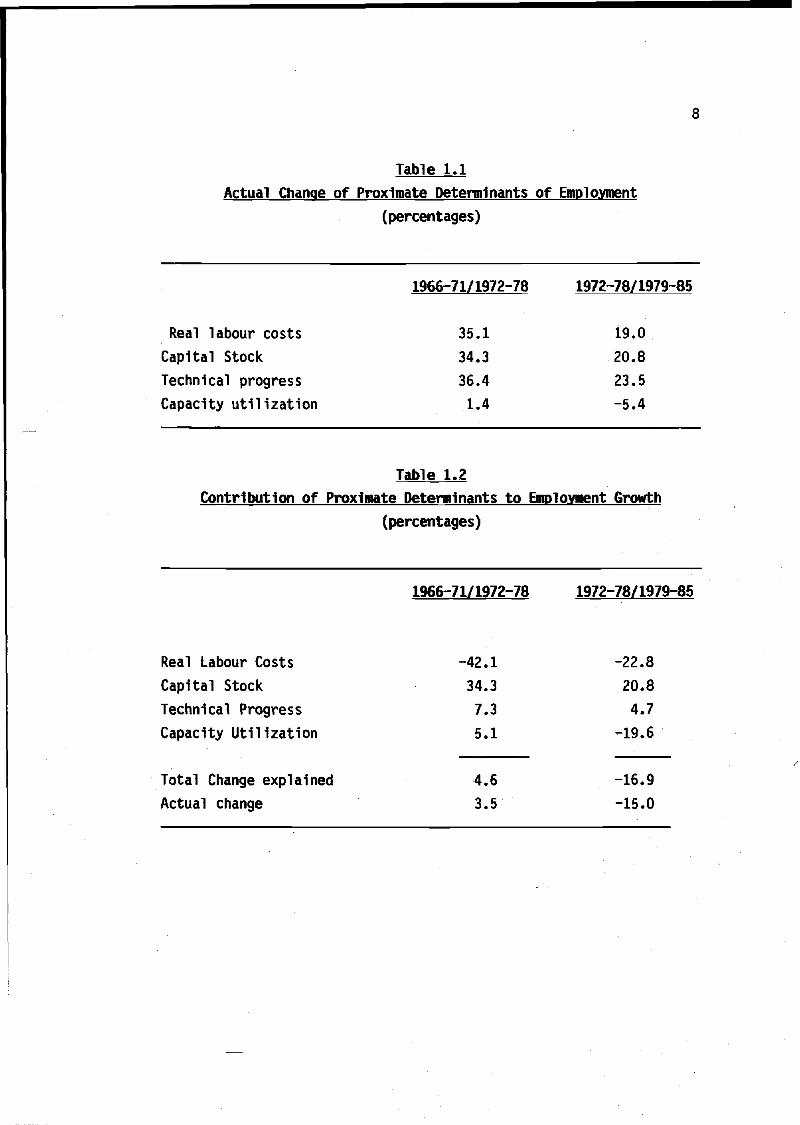
Table 1.1Actual Change of Proximate Determinants of Employment

(percentages)

Real labour costsCapital StockTechnical progressCapacity utilization

1966-71/1972-78

35.134.336.41.4

1972-78/1979-85

19.0

20.823.5-5.4

Table 1.2Contribution of Proximate Determinants to Employment Growth

(percentages)

1966-71/1972-78 1972-78/1979-85

Real Labour Costs -42.1 -22.8Capital Stock 34.3 20.8Technical Progress 7.3 4.7Capacity Utilization 5.1 -19.6

Total Change explained 4.6 -16.9Actual change 3.5 -15.0

FIGURE 1.5REAL GDP, EMPLOYMENT AND REAL LABOR COSTS

(ANNUAL RATES OF GROWTH).12

-1O- •

-.0»-

-.Oft-

.02-

ie«S19«6196719661»691»7O1»71 1872 19731974-1S761B7* 1>77 19781 «7» 19«01 »«1 1 »82198519O4-1»»5

PRODUCTIVITY,FIGURE 1.6

EMPLOYMENT AND REAL LABOR COSTS(ANNUAL RATES OF GROWTH)

.12

PRODUCTIVITY

EMPLOYMENT

COSTS

19«&19e818871»«»19O91»7O1»71 19721973 18741 676 I97Í 1977 1 97B 1979 1990 19«1 19821963196-41*86

10

1.6 show the annual rate of growth of real labour costs together withthat of employment, output and productivity. Leaving aside thepro-cyclical nature of real labour costs, perhaps the most remarkablefeature is their persistent increase during the second half of theseventies in the face of large falls of employment and very smallrates of output growth. However, there is a distinct deceleration oflabour costs in the last years of the period, which is clearly pickedup in Table 1.1.

Figure 1.7 shows the evolution of the rates of growth of theP

stock of capital and of its potential productivity . This figuresuggests the existence of a twenty-year cycle for the capital stockwhich was just completed in 1985. According to this interpretation,potential productivity would lead the rate of growth of the stock bysix to seven years. From 1965 to 1971, both the capital stock and itsmarginal productivity grew strongly. From 1972 to 1980, capital keptincreasing while potential marginal productivity declined reachingnegative rates of growth. This fall in productivity couid be thereason behind the big drop in the rate of growth of the stock after1974. By 1985 both variables have started to grow together again anda substantial recovery in the capital stock is expected . Table 1.1summarizes the behaviour of the capital stock, whose rate of growthbetween the period 1966-71 and 1972-78 was 34.3 per cent, while thatbetween 1971-78 and 1979-85 was 20.8 per cent. Table 1.1 also showsthat the index technical progress advanced more between the first twoperiods (36.4 per cent) than between the second and third (23.5 percent).

Finally, the index of capital utilization grew by 1.4 per centbetween the two periods, and fell by 5.4 per cent between the second

Potential productivity of capital is defined as the inverse ofthe capital to potential output ratio. Potential output, inturn, is defined as that level of output that would be obtainedat full capacity utilization. See below.

Fixed real investment grew 9.6 per cent in 1986, 14.5 per centin 1987 and is expected to grow around 12 per cent in 1988.

FIGURE 1.7CAPITAL STOCK AND POTENTIAL PRODUCTIVITY OF CAPITAL

(ANNUAL RATES ¿>r GROWTH)

11

YP/K

1986 1968 197O 1972 1974 1976 1978 19BO 1982 198+

FIGURE 1.8

CAPACITY UTILIZATION AND RATE OF GROWTH OF GDP.91

.73 J , ,_1965 1967

\

1 1 -I—19S9 1971

1 1 |1973 197»

-i (-1977 1979 1981

_l f-

GDP

CU

1985 198»

12

and third. Figure 1.8 plots the level of this variable and the rateof growth of output. The figure illustrates that this is a reasonablevariable to pick up the cycle, and that there is a clear fall indemand after 1975.

As can be seen in Table 1.2, the growth of employment betweenthe first two periods is largely explained by the increase ofcapacity utilization given that the negative effects due to thegrowth of labour costs is compensated by the positive effect of thecapital stock and technical progress. Similarly, the large fall ofemployment between the second and third period can be attributed tothe strong negative effect of cyclical demand (as proxied by capacityutilization), given that the smaller increase in labour costs isagain compensated by the weaker positive effects of the capital stockand technical progress.

1.2.2 Unemployment

The analysis so far, although instructive in order to see theeffect of labour costs, is unsatisfactory for two reasons: a) becauseit does not take into account factors that may have influencedunemployment via labour supply; and b) because it does not sayanything about what determines real labour costs and the capitalstock.

As we have seen in Figure 1.1, labour supply has been moreor less constant during the period in which unemployment hasincreased most. This, however, does not mean that labour supplyeffects have been absent in the determination of unemployment, asthey could have compensated one another as far as labour supply isconcerned. Also, we have identified the effect of labour costs onemployment, but real labour costs are endogneous to the model anddepend on all factors that determine the wages workers desire and thewages employers are prepared to pay.

13

We have been able to estimate the influence on unemployment ofsome of these factors and the overall results are promising. We haveidentified significative influences from Social Securitycontributions, indirect taxes and real import prices; that is, threeof the four elements (the fourth being direct taxes) that form thewedge between real labour costs and the consumption wage. Also, anindex of mismatch in the labour market, the replacement ratio and aproxy for union pressure show up as having significant effects on thelevel of unemployment.

Another satisfactory result of this exercise has been that wehave not been able to reject the hypothesis of absence of long-runeffects of the capital-labour ratio and of technical progress onunemployment. The strong effect of the capital stock on employmentdiscussed above should in theory be compensated by an equivalent andopposite effect coming from the labour force so that there is nolong-run influence on unemployment. The data clearly accept therestrictions implied by this hypothesis.

Table 1.3 shows the actual changes of the variables determiningdesired and feasible wages. We see that there has been a fairlysteady increase in Social Security contributions (although in thelast years they are practically stable), and a moderate fall inindirect taxes (although since 1983 they are rapidly increasing). Theimport price wedge has gone down by -3.9 per cent between the firstand second periods, and up by 1.9 per cent between the second andthird periods. The evolution of technical progress and capacityutilization has already been described in Table 1.1. The mismatchindex has grown less between the third and second periods thanbetween the second and the first, reflecting an improvement in theoccupational structure, whereas the replacement ratio shows anopposite and much higher pattern of growth. The growth of the unionpressure dummy has, by construction, opposite signs and the sameabsolute value in the two comparisons, increasing between the firsttwo periods and falling between the second and third. Finally, we see

14

that the capital labour ratio has increased substantially throughoutthe whole period, although, as expected, there is an importantdeceleration after the first oil crisis.

Table 1.4 shows the contribution of these variables tounemployment. Between the first two periods, of the six wage pushfactors, Social Security contributions, followed by the unionpressure variable are the main contributing factors, while theincrease in capacity utilization helped to moderate the rise inunemployment. The mild negative effect of the import price wedge isexplained by the policy of subsidising the domestic price of energyafter the first oil crisis, a policy which disappeared when thesecond oil price shock occurred. Concerning the comparison betweenthe last two periods, we see that the effect of Social Securitycontributions is slightly larger than that of the previouscomparison. In addition, the replacement ratio becomes a moreImportant contributing factor, while the indirect taxes and the unionpower dummy help to moderate the increase in unemployment. Cyclicaldemand (as proxied by capacity utilization) now becomes stronglycontractionary and exerts, by far, the most important influence onthe rise of unemployment.

According to these results, therefore, cyclical demand appearsas the major explanatory factor of the recent evolution ofunemployment in Spain. Had capacity utilization remained constantthroughout the whole period under consideration, unemployment wouldhave Increased by about 4 and a half points between the first andsecond periods and by about 3 points between the last two. This givesa total rise of 7.5 points, which is much lower than the 14 pointsrise obtained after considering the effect of demand.

15

Table 1.3Actual Change of Variables Determining Desired and Feasible Wages

(percentages)

1966-71/1972-78

Social Security contributionsIndirect taxesReal import prices*Capital -Labour ratioTechnical progressCapacity utilizationReplacement ratioMismatchUnion power dummy

4.41.3

-3.927.836.41.4

3.01.171.4

1972-78/1979-85

5.2-0.61.3

24.923.5-5.4

7.60.4

-71.4

*Weighted by share of imports in GDP.

Table 1.4Explanation of Actual Unemployment

(percentage points)

1966-71/1972-78

Social Security contributionsMismatchIndirect taxesReal import prices*Union power dummyReplacement ratioCapacity utilization

Total change explainedActual change

2.30.50.7-0.31.00.4-2.2

2.43.5

1972-78/1979-85

2.80.2-0.3

0.1-1.01.08.6

11.410.9

*Weighted by share of imports in GDP

16

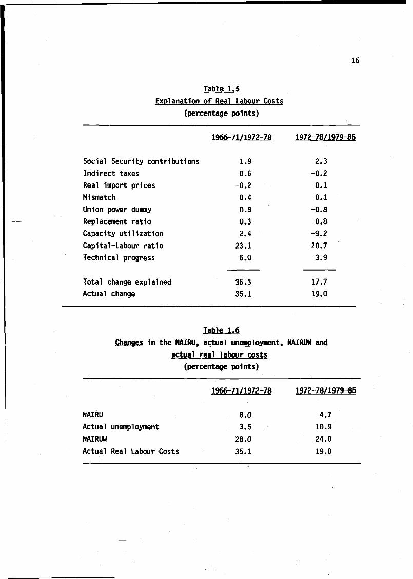
Table 1.5Explanation of Real Labour Costs

(percentage points)

Social Security contributionsIndirect taxesReal import pricesMismatchUnion power dummyReplacement ratioCapacity utilizationCapital -Labour ratioTechnical progress

Total change explainedActual change

1966-71/1972-78

1.90.6-0.20.40.80.32.4

23.16.0

35.335.1

1972-78/1979-85

2.3-0.20.10.1-0.80.8-9.220.73.9

17.719.0

Table 1.6Changes in the NAIRU. actual unemployment. NAIRUW and

actual real labour costs(percentage points)

NAIRU

Actual unemploymentNAIRUWActual Real Labour Costs

1966-71/1972-78

8.03.528.035.1

1972-78/1979-85

4.7

10.924.019.0

17

Table 1.5 repeats the previous exercise to explain the actualchange in real labour costs. Between the first two periods, reallabour costs grew 6.2 points in excess of what would be explained byproductivity factors (capital-labour ratio and technical progress).Of these 6.2 points, the wedge between real labour costs and theconsumption wage explains 2.3 points (mostly due to Social Securitycontributions, which alone explain 1.9 points), cyclical demand 2.4points, and the push factors (mismatch, union power and thereplacement ratio) the other 1.5 points. Between the second and thirdperiods, on the other hand, real labour costs grew 6.9 points lessthan what would be justified by productivity. Here push factorsplayed practically no role, as the depressing effect of union powerwas fully compensated by the positive effect of the replacementratio. The main explanatory factor of the fall in labour costs wascyclical demand, which induced a large fall of 9.2 points, more thansufficient to compensate the 2.2 rise due to the wedge. We have thenthat, according to these results, demand management has been acrucial factor for explaining both the substantial rise inunemployment and the control of labour costs (and thereforeinflation).

What are the implications of these results for thenon-inflationary rate of unemployment (NAIRU)? The main ones can begathered from Table 1.4, as the change in the NAIRU can be deducedfrom the figures presented there, excluding the influence of cyclicaldemand whose l:vel is set equal to the value taken during thebaseline period. This gives the changes shown in Table 1.6. Accordingto these results, the NAIRU would have grown more than actualunemployment between the first two periods (8.0 points versus 3.5points respectively), but less between the last two periods (4.7points versus 10.9 points). Similar considerations can be made withrespect to the rate of growth of labour costs which is consistentwith the NAIRU (NAIRUW). Between the first and second periods thechange in the NAIRUW was about 7 points lower than the actual change

18

FIGURE 1.9UNEMPLOYMENT AND NAIRU

23.O

20.7-

a.z -

NAIRU

/

/

-t- -+- -t- -t- _t_ -»- -t- •+• -+- -»- -+- -t- -t- -f- -»-1046 1««7 10M 1»6« 1»7O 1971 1972 1O73 1«74 1O75 1»7G 1B77 107* 1079 108O 1981 1»»2 1»»3 1044 1060

19

in real labour costs whereas between the second and third periods itwas 5 points higher.

Figure 1.9 presents the same information, but showing the levelof the NAIRU and its annual evolution4. We observe that the NAIRU hasincreased substantially over the whole period and has stayed above ornear actual unemployment for most of the sample period. It is onlyafter the beginning of the 80's that the NAIRU begins to slow downits rate of increase, to end in 1985 3.6 points below actualunemployment. It must be noted, however, that these conclusions aresomehow sensitive to the period used to define the initial value ofthe NAIRU. Had this been defined as the average of actualunemployment for the period 1966-73, then the NAIRU would have been4.2 points below the actual rate in 1985. For this reason, we feelthat the information about changes across periods given in Table1.6 may be more relevant than the plots of Figure 1.9.

.2.3 Demand and Capital constraints

In the previous sections we have seen that both cyclical demandand the capital stock have been relevant factors in the determinationof Spanish unemployment. The stock of capital has played an importantrole in labour demand, and capacity utilization (our proxy forcyclical demand) seems to have had a significant influence on thefeasib.e wage. Now we want to turn back to these two variables butfrom another perspective.

The stock of capital sets the size of the productive capacityand, therefore, establishes a limit to the amount of workers thatcould be employed when using fully this capacity. In the long run,with flexible relative prices, this capacity should adjust toaccommodate the available labour supply, but in the short run, a

4 The slightly peculiar evolution during the period 1973-1977 isdue to the transitory effect of the step dummy proxying unionpressure.

20

given capital stock may impose an effective restriction to the amountof workers that can be employed even in the presence of sufficientdemand. It is important therefore to find out to what extentunemployment is due to a deficient use of the available capacity, andby how much could employment increase if this capacity was fullyused. For this purpose we define the concept of potential employmentas the level of employment corresponding to full use of the availablecapital stock.

As far as demand is concerned, we could be in a situation inwhich altough there is capacity, the level of demand is so small thatthere is no incentive for firms to use fully the capital stockavailable. In this situation, aggregate demand sets the effectiveconstraint to employment. It is therefore instructive to identifyalso the extent to which this circumstance has been relevant inexplaining the recent evolution of the labour market, and for thispurpose we define the concept of Keynesian employment as the levelof employment corresponding to full satisfaction of u_,nand fordomestic output.

Figure 1.10 plots the evolution of potential employment (LP),Keynesian employment (LK), labour supply (LS) and observed employment(L). Potential employment follows an increasing trend until 1975,growing at an annual rate of 0.7 per cent, and then fallsmonotonically for the rest of the period, at an annual rate of 2.0per cent. This pattern can be explained by the evolution of theoptimal labour-capital ratio, given relative factor prices andproduction conditions, and by the evolution of the capital stock.Table 1.7 shows the contribution of these two factors. From 1965 to1975, the increase of the capital stock was 49.3 per cent and that ofthe optimal labour-capital ratio -41.7 per cent, which sums up to theestimated increase of potential employment of 7.4 per cent. From 1975to 1985, the optimal labour-capital stock maintained a similar rateof decline, but the capital stock grew much less than in the previous

21

period, not being able therefore to absorb the amount of workersfreed by the much lower requirement of labour per unit of capital.

TABLE 1.7

Decomposition of the Growth of Potential Employment

(percentages)

1965 - 1975 1975 - 1985

Optimal labour-capital ratio -41.7 -42.3Stock of capital 49.3 22.2

Potential employment 7.4 -20.1

We have then that what really explains the evolution ofpotential employment, is not so much the changes experienced by thefactor mix, which maintained a uniformly decreasing trend over thewhole period, but the much lower rate of increase of the capitalstock after 1975. Figure 1.7 above shows this deceleration in thestock of capital.

Keynesian employment follows a similar pattern as potentialemployment, although much more cyclical and reaching the peak twoyears earlier (1973). From 1965 to 1973 Keynesian employment grew atan annual rate of 1.4 per cent, while form 1973 to 1985 it fell at anannual rate of 2.3 per cent. Here again, the evolution of this typeof employment depends on two factors: the evolution of demand fordomestic output and the evolution of the labour-output ratio. Table1.8 shows that in this case the main reason for the big fall inKeynesian employment in the period 1973-85 is not the improvementproductivity (it in fact decelerated in the second period with anannual rate of increase of 3.9 per cent as compared to 4.4 per centin the first), but the dramatic fall in demand for domestic output,

22

which 1n the period 1965-1973 grew at an average annual rate of 5.7per cent while in the period 1973-1985 grew only at an average annualrate of 1.7 per cent.

TABLE 1.8

Decomposition of the Growth of Kevneslan Employment(percentages)

1965 - 1975 1975 - 1985

Demand for domestic output 45.8 20.3Labour-output ratio -35.5 -47.8

Keynesian employment 10.3 -27.5

Another interesting feature of Figure 1.10 is the relation thatLP and LK keep with one another and with observed employment (L) andlabour supply (LS). In this respect we can distinguish three periodswhich roughly coincide with the ones used in the previous section.From 1965 to 1971, LP and LK keep what we consider a normalrelationship, with LK above LP in the peak of the cycle and viceversain the trough. Besides, both LP and LK are above labour supply andemployment, thus indicating a fairly well functioning economy whereactual employment was very near labour supply and existed a certainamount of excess demand for labour, which in 1970 represented a 2.5per cent of the labour force. From 1971 to 1978 the relationshipbetween LP and LK is more or less maintained, but LP, practically forthe whole period, stays below labour supply, which can be interpretedas a signal of the appearance of some limitations as far as theamount of available capital is concerned. Also, after the peak of1973 and towards the end of the period, we observe a clear weakeningof Keynesian demand for labour, which ends up in 1978 at a level 2.0per cent below labour supply. The last period, 1978-1985 is

FIGURE 1.10L, LS, LP and LK

23

I3SOO-

130DO-

12ODO- •

1160O-

10600-

LS

._ LP

LK

980O-1 1 1 | 1 1 1 1 ( 1 1 1 1 1 1 1 1 1 1 1 (.10«S 196S 1»67 1MB 1SS6 107O 1971 1»72-1973 1«7* 1976 197S 1»77 1«78 1979 19«0 19«1 1»»2 1«W 16E4 1MB

FIGURE 1.11REGIMES SHARES

1.0

19«7 19«9 1971 1973 1975 1977 1979 1961 1983 19B5

24

completely different from the other two, and picks up the very strongeffects of the crisis upon employment. Here, LP stays above LK allthe years, thus suggesting that the main constraint to employmentgrowth has been deficient demand, which by 1985 was requiring a levelof employment 21.9 per cent below that of labour supply. However,according to our results, demand expansion alone could not havesolved this problem as the extra employment required would very soonhave met the capital constraint. In 1985, without increasing thecapital stock, the maximum amount of employment would still have been18.9 per cent below labour supply.

In order to analize the incidence of the different constraintson the evolution of actual employment we have decomposed its rates ofgrowth in four layers. These layers go from endogenous determinantsto more exogenous ones.

Layer one is presented in Table 1.9. The observed rate of growthof actual employment is decomposed as the rate of growth of thepotential labour-output ratio (i.e. the inverse of potentialproductivity) plus the rate of growth of observed output plus aresidual coming from the neglected cross-products and thesubstitution of potential productivity for the observed one. Theaverage of potential productivity in 1972-78 was 32.3 per cent higherthan the average in 1966-71, while the average in 1978-85 was only27.8 per cent higher than in 1972-78. Therefore the fall inemployment in the last subperiod is not explained by the evolution ofproductivity, but by the large fall in output growth. Output grewonly 12.7 per cent in 1979-85 with respect to 1972-78, and was unableto offset the effects of productivity growth as it did in 1972-78when compared with 1966-71.

Next we decompose output growth as determined by Keynesiandemand, full capacity (or potential) output and full employmentoutput. At any given moment of time firms produce what they produce,and no more, because they are restricted either by demand or by

25

TABLE 1.9

DECOMPOSITION OF CHANGES IN EMPLOYMENT

Effects of potential productivity and output growth(percentages)

1972-78/1966-71 1979-85/1972-78Estimated change in potentialproductivity of labour 32.3 27.8

Actual change in output 35.2 12.7

Explained change in employment 2.9 -15.1

Actual change in employment 3.5 -15.0

26

capacity or by the availability of labour supply. Therefore thegrowth in output is explained by the growth in demand in thedemand-restricted firms, the growth in capacity in the capacityrestricted ones and so on. This second layer is presented in Table1.10.

Keynesian demand grew, as an average, 35.9 per cent in 1972-78with respect to 1966-71. However, its contribution to output growthwas 10.7 points because roughly a third of firms were demandconstrained. Full capacity output grew 34.7 points in that period andits contribution to output growth was 17.4 points, as roughly half offirms were capacity constrained. Full employment output grew 38.9points, as only a sixth of firms were labour-supply constrained. Theannual evolution of regime shares of firms is shown in Figure 1.11.

When we compare the average of the period 1979-85 with theaverage of 1972-78 we see that Keynesian demand grew an 11.4 per centand its contribution to output growth was 8.6 points, reflecting thatthree fourths of firms were demand constrained in this period. Thecontribution of potential output was 3.6 points, less than one fifthof its growth, and the contribution of full employment output wasless than one tenth of its growth. The most generally bindingconstraint in this period is the demand one, followed closely bycapacity restrictions if we consider the situation depicted in Figure1.10. By the end of the period the labour supply constraint wasalmost negligible (see Table 4.7 or Figure 1.11).

In the third layer we address the decomposition of Keynesiandemand, potential output and full employment output. Table 1.11 showsthe changes in consumption, investment, government expenditure andnotional external balance. The comparison of the two columns of Table1.11 reflects the slowdown of the economy in 1979-85. Consumptionfell from a growth of 35.5 points to 11.3, diminishing itscontribution to Keynesian demand growth in 16.4 points. Investmenthad a negative contribution of 2.8 points in the last period compared

27

TABLE 1.10

DECOMPOSITION OF OUTPUT GROWTH

Estimated changes of output growth determinants(percentages)

1972-78/1966-71 1979-85/1972-78

Keyneslan demand 35.9 11.4

Full capacity output 34.7 15.4

Full employment output 38.9 26.2

Contributions to output growth(percentages)

1972-78/1966-71 1979-85/1972-78

Keyneslan demand 10.7 8.6

Full capacity output 17.4 3.6

Full employment output 7.8 2.6

Explained output growth 35.9 14.8

Actual output growth 35.2 12.7

28

to a positive one of 8.4 points in the middle period. Governmentexpenditure proved fairly constant both in its own rates of growthand in its contribution to Keynesian demand growth. The notionalexternal balance contributed decisively to sustaining demand in thelast period, contributing 3.5 points to demand growth while, in themiddle period, it had only contributed 0.5 points.

In Table 1.12 we decompose potential output in terms ofpotential productivity of capital and the capital stock. Both ratesof growth are depicted in Figure 1.7 on an annual basis. The fall inthe estimated change of potential output in the last period is dueboth to the fall in the rate of growth of capital and to the fall inthe potential productivity of capital which seems to be a sort ofleading Indicator of the former (see Figure 1.7). In the last periodthe capital stock grew 13.5 points less than in the middle period andpotential productivity of capital grew at a negative rate of 5.4 percent.

Full employment output is decomposed in Table 1.13 in terms oflabour supply and potential productivity of labour. The slowdown offull employment output is accounted for both by the decelaration ofpotential productivity growth and by the diminishing labour force inthe last period.

Finally, the fourth layer decomposes the changes in potentialproductivity of labour in terms of the effects of relative prices andtechnical progress. As can be seen in Table 1.14 both effects operate1n the same direction in determining the deceleration of potentialproductivity growth. The growth of the cost of labour with respect tothe cost of capital has been 6 points less 1n the last period than inthe middle one, but the contribution of relative prices of labourproductivity growth was only 3 points less in that period than in theformer. Technical progress also slowed down in the last period,diminishing its contribution to productivity growth from 18.5 points1n the middle period to 12.8 1n the last one.

Annual figures for the four layers are included in an Appendix.

29

TABLE 1.11

DECOMPOSITION OF KEYNESIAN DEMAND GROWTH

Actual Change in Keynesian Demand determinants

(Percentages)

1972-78/1966-71 1979-85/1972-78

Consumption 35.5 11.3

Investment 35.2 -11.6

Government expenditure 33.9 31.3

Notional exports(*) 60.1 41.5

Notional Imports (*) 55.1 26.3

Contributions to Keynesian Demand growth

(Percentage)

1972-78/1966-71 1979-85/1972-78

Consur.rt1on 24.0 7.6

Investment 8.4 -2.8

Government expenditure 2.9 2.7

Notional external balance 0.5 3.5

Explained growth ofKeynesian demand 35.8 11.0

Estimated change ofKeynesian demand 35.9 11.4

(*) Estimated

30

TABLE 1.12

DECOMPOSITION OF FULL CAPACITY OUTPUT

(Percentages)

1972-78/1966-71 1979-85/1972-78

Actual change in capital stock 34.3 20.8

Estimated change In potentialproductivity of capital 0.4 -5.4

Estimated change in potential output 34.7 15.4

TABLE 1.13

DECOMPOSITION OF FULL EMPLOYMENT OUTPUT

(Percentages)

1972-78/1966-71 1979-85/1972-78

Actual change in labour supply 6.6 -1.6

Estimated change in potentialproductivity of labour 32.3 27.8

Estimated change in full employment 38.9 26.2Output

31

TABLE 1.14

DESCOMPOSITION OF POTENTIAL PRODUCTIVITY OF LABOUR GROWTH

Actual changes in potential productivity determinants(Percentages)

1972-78/1966-71 1979-85/1972-78

Relative prices 32.4 26.4Technical progress5 36.4 23.5

Contributions to potential productivity growth(Percentages)

1972-78/1966-71 1979-85/1972-78

Relative pricesTechnical progressExplained change in potentialproductivity of labour

Estimated change in potentialproductivity of labour

15.918.5

34.4

32.3

12.912.8

25.7

27.8

Estimated

32

2. THE MODEL

High inflation and falling employment are the two main featuresof the recent stagflation period. Any suitable model of stagflationmust address these two issues. In this section we present a sketchof the theoretical model used in this paper and based on the work ofLayard and Nickell (1985), Sneessens and Dréze (1986) and Sneessens(1987). The empirical framework used and the results obtained arepresented in later sections.

Inflationary pressures are mainly caused by distorsions inthe distribution mechanism. Changes in the bargaining power of unionsand firms over the distribution of income lead, in a non-cooperativesetting, to inflationary pressures in the short-run and unemploymentin the long-run. Monopoly power on wage and price determination is afeature of our economies and lies behind the so called inflationarybias.

Employment, on the other hand, is affected by a variety offactors. It would be too naive to identify a single cause of theemployment slump. The Second Generation Disequilibrium Modelsconstitute a useful framework to assess the relative importance ofdifferent factors such as: capital shortages, low agrégate demand,labour supply developments, structural mismatches and long-runpermanent changes in relative prices . A simple version of this typeof models is presented in the last part of this section. Given theimportance of the determinants of aggregate demand, especiallyinvestment, the labour market block must be enlarged to account forthe evolution of investment, consumption, trade balance, etc. and the

By Second Generation we mean the set of models in which anoverall disequilibrium regime characterising the economy at apoint in time is substituted by a distribution of regimes acrossmarkets which hence can suffer from different disequilibriumsituations (see e.g. Muellbaur and Winter (1980)).

33

initial model becomes an small (albeit non-fully complete) macromodel.

The main assumptions of the model can be summarized as follows.

i) Firms and workers (unions) set wages before prices andemployment are known. Bargaining refers only to expected realwages (W/Pe) and the firm keeps the right to decide about pricesand employment.

ii) There are n firms which operate in a monopolistic competitionset up. Each firm faces a downward sloping demand curve on itsprice relative to the aggregate price level d(Pj/P). Aggregatedemand is given by YD. The firm sets its price as a mark-up overnormal unit costs, taking into account the expected price of itscompetitors (in aggregate, Pe), before the actual value of theexogenous demand (e ), capacity (ej) and labour supply (v )random disturbances are known.

iii) Technology is of the putty-clay type, with large ex-antesubstitution possibilities and fixed ex-post factor proportions.Assuming separability, the firm's value added is subject to thefollowing short run constraints (Sneesens (1987)):

Pi YDYÍ * d (—) ej (2.1)

Pe n

Y-j < A-LSi Vi (2.2)

YÍ <. B-Kj e-j (2.3)

r34

The firm chooses ex-ante the optimal technical proportions(A,B) and capacity (K-f) to minimize long-run costs. LS-¡ is thelabour supply exogenously given to the firm. In most of thepaper we shall take K^ as given by past investment decisions sothat we shall focus on the choice of A and B.

iv)

v)

Labour is the only variable factor and it is choosen once Pj/P,e-ji vj, ej are known. Given the ex-post rigidity, the employmentfunction is simply:

LT = A'1 YÍ (2.4)

Finally, we will consider a large number of firms, so thatsample moments are equal to population ones.From now on we define as YD^, YSj, YPj as the right hand sidesof (2.1), (2.2), (2.3) respectively.

2.1. Wages and Prices

Prices (Feasible mark-up)

Given the stochastic structure of the model we shall assumethat each firm sets its price as a mark-up over normal unit costsdefined at the full employment level of resources (E(YP )/E(LSj)).Firms also take into account the expected rival's price and henceprices are set according to:

PI = h ( u.W.-Ed-Sj)

E(YPi)Pe) (2.5)

where u is the mark-up and E(LS-¡) represents the expected availablelabour force and E(YPj) the expected output at full capacity orpotential output as defined in (2.3). If we assume (Nickell (1986))

35

that h is homogeneous of degree one on both arguments we can rewrite:

Piw = u

E(LSi)

E(YP!)• h (— P 1 )p.' (2.6)

The mark up will usually be a function of cyclical demandpressure which we will represent by:

E(YDi)y ( )

E(Yi)(2.7)

The sign of u'() is ambiguous, and several reasons can be foundin support of either a positive reaction or a negative one. Among themain factors behind the explanation that the mark-up movesprocyclically lies the increase in marginal costs as demand expands.Among the models that imply a countercyclical movement we can find,in the context of oligopolistic industries, theories based upon theview that collusion is more dificult when demand is high (seeRotemberg and Saloner (1986)) or on the attraction of more"unattached" customers, which increases the elasticity of demand (seeBils, (1985)).

If we now assume point expectations, and given that the randomdisturbances are distributed with mean equal to one, we can write:

YDi

Yi= & (DUK) Q'> 0 (2.8)

YPj

LSi

Kj

LSi(2.9)

36,

where DDK is the degree of capital utilization.

Aggregating over firms and taking logs, our price equationis as follows

p - w = OQ - «i (p~Pe) - 012 duk ~ a3 (k~ls) (2.10)

where lower case letters denote logs, and the coefficients arepositive except 012 which, according to._ the previous discussion, canbe either positive or negative.

Real Waoes (Desired mark-up)

We obtain our wage equation as the outcome of a bargainingprocess over ex-ante desired real wages. There is no uncertaintyabout the rival's fall back position so that the outcome can bethought of as coming from a Nash bargaining type model:

w - p = Po - Pi (P-P6) - P2 U + P3 (k-ls) + Z (2.11)

where U is the unemployment rate and Z is a vector of push factorsincluding the replacement ratio (rr), union power (PS), and thevariables driving a wedge between the producer's price (p) and theconsumer price index. Among these we find the income tax (t2)>indirect taxes (t$) and Social Security contributions (ti),as well assome function of the ratio of imported goods prices over the CPI,(Pm-F).

Z = Z (rr, PS, (Pm - P), ti, t2, t3) (2.12)

37

Inflation and the distribution of ir-come

Solving out (2.10) and (2.11) under the assumptions that

03 * <*3

P - Pe * A2 P (2-13)

we get the following unemployment-inflation trade-off .

1 1 <x2 1U = (p0 + OQ) (Pi + <*l) A¿P (duk) Z

P2 02 03 P2(2.14)

Expression (2.14) has the conventional Phillips Curveinterpretation where distributional factors are explicitly allowedfor. It is not a theory of unemployment, for it involves otherendogenous variables such as A p and duk. What this expression showsis how much inflation is required to make the desired and feasiblemark ups consistent for a given level of unemployment and demandpressure. If we want to turn (2.14) into an operative theory ofinflation we need independent explanations of unemployment anddemand. This is the main subject of the next pages, although thistask is only partially carried out. As we shall see we only explainone side of the unemployment rate leaving the labour supplyexoge. jus; similary demand pressure is explained in terms of a set ofvariables some of which are themselves endogenous (mainly duk).

Equation (2.14) captures the underlying inflationary pressureof an economy. In particular, it gives the amount of unemploymentneeded to keep inflation constant; i.e., the NAIRU. Keeping inflationconstant makes not only consistent the desired and feasible actualmark-ups, but the actual and perceived ones too. The determinants of

The underlying idea behind the approximation used for the pricesurprise is that the rate of inflation follows a random walk, ahypothesis which is not rejected by the data.

38

the NAIRU are the ultimate causes of inflation and (2.14) shows towhat extent inconsistent distributional demands could lie behind theinflationary bias of an economy.

Figure 2.1 gives an idea of the inflationary impact of a supplyshock represented by an increase in any of the push factors in Z. Ifwe start in a long-run equilibrium at EJ with p = pe (or A2p= 0), anincrease in Z shifts the wage equation rightwards.

In the short run (for a given U at NAIRUi) inflation must riseto make compatible the new distribution on expected terms. Noticethat workers are pushing for higher real wages and the firm tries torecover costs, at least partially, through price surprises. Thisoffsetting behaviour cannot be taken too far, for it may weaken thefirm's position in the goods market, and this leads to a situationlike E'i in which everybody accepts their expected income, althoughworkers are getting in real terms less than what they believe .

W-PFISURE 2.1

AZ

NAIRU, NAIRU0

39

This situation is not a stable one. In the long-run actual andperceived incomes cannot differ and the only way in which the newincome distribution can be made acceptable to workers is at a higherunemployment level such as NAIRU2- In other words, a depressingeffect on union's bargaining position (achieved through the rise inunemployment) must follow the increase in Z if firms are to keeptheir mark-up without accelerating inflation.

The wage-price formation mechanism just described is the crucialelement of the theory of inflation contained in this model. However,it is also an explanation of the evolution of relative factor prices,which are the main determinants of the technological and investmentdecisions described the employment block.

Unfortunately, we do not have at this stage a model to explaineither the price of investment goods, nor the user's cost of capital.These are considered exogenous to avoid the explicit -lodelling of thefinancial sector and the investment goods market. Therefore, in whatfollows, any impact of relative factor prices should be understood asbeing caused by changes in the underlying push factors in wage andprice formation.

40

2.2. The determinants of employment

The Production Function

The joint choice of factor proportions and firm's size is theoutcome of the following cost minimization problem (Gagey, Lambertand Ottenwaelter (1987)), where ex-ante substitution possibilitiesare represented by a CES function:

Min (W LPi + CC KÍ) (2.15)

s.t.

fi T R TYPi = ( T (e L LPi)'01 + (1-T) (e k W~a )~1/ct (2.16)

where U and CC are the nominal wage rate and user cost of capitalrespectively, LP-¡ is the level of employment corresponding to a fullutilization of K-j, which is required to produce YP-j. Finally, P|_ and0k are the labour and capital augmenting technical progresscoefficients, and T is a time trend.

Assumming that in the long-run prices are set as a mark upover total unit costs, the first-order conditions result in thefollowing expressions:

KÍ 1-T _ P.- PK (l-o T W( )a e L K (—)a (2.17)

LPi T CC

YPi (!-<0PkT CC a(1-T)° e (—) (2.18)

Ki P

where

«•TÍr

41

Equation (2.17) determines the optimal capital-labour ratio, and(2.18) can be interpreted either as an investment function or as acapacity (YP-j) equation (we will come back to this point).

FIGURE 2.2

Given constant returns to scale, to find out the desired level oflabour (LPf), we need to fix either K-j or the desired capacity (YPj).In the long-run K-j is going to be endogenous, and we shall establisha target capacity level which will turn (2.18) Into an investmentfunction. In the medium term however, we consider the installedcapacity as predetermined and therefore (2.17) and (2.18) give us theoptimal capital/labour ratio (K-j/LP-j) and capacity level (YP-j).This 1s shown diagramatically in Figure 2.3.

FIGURE 2.3K.

\

42

Expression (2.17) is therefore the potential labour demandconditional on the capital stock:

LPi - A'1 B KÍ (2.19)

where

1 K1 • w

A.B l = ( ) = g (T, 6(A)( )) (2.20)LPi CC

where actual (W/CC) has been substituted out by a distributed lag9(A) (where .A. is the lag operator) of relative prices. This worksas a proxy for relative price expectations as determinants of theex-post fixed proportions decisions. Notice that (2.19) and (2.20)look very much like a classical labour demand equation, in whichrelative prices do not have an inmediate impact given the sluggishtechnological adjustment. The smaller the mean lag in 8(-A_), thecloser the model to a conventional putty-putty competitive labourdemand equation. We can also write LP-j as a function of YPj:

LPi = A'1 YPi (2.21)

Eaplovaent Function

So far we have obtained an expression for labour demand when thefirm is only constrained by its past investment decisions. However,the firm can also be either unable to sell all its output or to hireas much labour as it wants to. Therefore these two other constraintsmust also be taken into account.

43

FIGURE 2.4

Classical Regime

Keynesian Regime

Repressed Inflation

The conventional representation of the three employment regimes,such as that shown 1n Figure 2.4, Is no longer approplate here, for1t 1s based on a putty-putty technology. Nevertheless, 1t 1s easy togain some intuition of the short run employment decisions of the firmas follows.

At a given point in time, t, the firm takes K^, A and B asgiven, and therefore there are no substitution possibilities. Theproduction set is then represented by right angle Isoquants as inF1g. 2.5.

FIGURE 2.5

LP.

44

If there are no constraints elsewhere, labour demand must liealong the ray through the origin. Clearly, installed capital is thebinding constraint. Employment is then given by the labour demand(ID^) at its potential level.

LÍ = LD-j = LPi = A"1 B KÍ if LDi < LSiYPi < YDi

(2.22)

Let us consider now the possibility of the firm being in asales constraint. Once prices are set and e-j and YÍ are realized, itmay be the case that the firm's demand (YD-¡) falls short of YP-j. Ifthat is the case, employment is no longer given by (2.22) but

LÍ = LDi * LKi = A"1 YDi if LDi < LSiYPj > YDi

This is the situation portrayed in Fig. 2.6:

(2.23)

FIGURE 2.6

KU.

45

where KU-j stands for used capital, and where we assume that thedegree of labour hoarding is constant so that effective labour inputis a constant proportion of employment . For the case of no rationingin the labour market, employment is given by the labour demand side,which can be represented in a more compact fashion by the traditionalmin condition,

LÍ = LDi = min (LPj, LK^), if LDj < LSi , (2.24)

which can also be written as,

LÍ = LDi - A"1 (min (YPi, YDi)) (2.24')

If the number of firms is very large, the aggregate demand for labouris given by:

L = LD = nE(LDi) = nA"1 E(min (YP , YDn-)) (2.25)

Under some assumptions about the joint distribution of e-j, e-¡, it canbe shown (Lambert (1987)) that (2.25) can be written as

-*, -*, -1/6!E(min (YP1f YDi)) = (E(YDi) 61 + E(YPi) 6* ) (2.26)

where (l/6i) is an increasing function of the variances andcovariances of the stochastic vector. Proceeding in the same way forEÍYDf), EÍYPí), E(Ki), (2.26) can be written as

LD - ( (A'1 YD)~61 + (A BK)"6! ) : (2.27)

ft0 This is assumed for simplicity. The whole argument would stillgo through in the presence of varying labour hoarding.

48

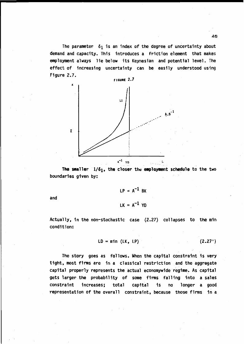
The parameter 6 is an index of the degree of uncertainty aboutdemand and capacity. This introduces a friction element that makesemployment always lie below its Keynesian and potential level. Theeffect of increasing uncertainty can be easily understood usingFigure 2.7.

FIGURE 2.7

LD

A.B-1

A"1 yo

The smaller l/6i, the closer the employment schedule to the twoboundaries given by:

andLP = A"1 BK

LK = A l YD

Actually, in the non-stochastic case (2.27) collapses to the mincondition:

LD = min (LK, LP) (2.271)

The story goes as follows. When the capital constraint is verytight, most firms are in a classical restriction and the aggregatecapital properly represents the actual economywide regime. As capitalgets larger the probability of some firms falling into a salesconstraint increases; total capital is no longer a goodrepresentation of the overall constraint, because those firms in a

47

Keynesian regime drive the employment schedule leftwards. It shouldbe clear that in the non-stochastic case all firms are in the sameregime and so employment must be given by either LP or LK. Similarly,as the variance of the shocks gets higher, for a given predominantregime, the proportion of firms in the alternative regime increases,and hence the whole employment schedule shifts to the left. At amacroeconomic level these stochastic disturbances mainly representstructural shifts and relative price changes among sectors.

So far we have been dealing with a labour market that shows norationing. When the labour supply lies, at the prevailing real wage,below the labour demand, employment is given by the labour supply.Therefore,

LÍ = min ( LDi, LS^) (2.28)

Following the same steps as before, the aggregate employment functiontakes the form

-1/02L- ( (LO) "62 + (LS)-«2 ) (2.29)

where (1/62) is an increasing function of the variances andcovarianees of the stochastic vector (e , e^, v ). It representsthe degree of labour market mismatch between demand and supply, whichIntroduces an additional friction. The larger the mismatch (1/62)»the smaller the observed employment for given levels of demand andsupply. Figure 2.8 represents diagramatically this case.

FIGURE 2,8

LD

/

XX//

48

The employment function can then be written as in Gagey,Lambert, Ottenwaelter (1987),

L =«2/«lr - «1 - « 1 1 ¿/ L ~ «2

[ (LK) + (LP) J + (LS)-l/62

(2.30 )

Q

and assuming that 61 = 62 -P

I = [ (A'1 YD)~f + (A BKrf + (LS)~P] (2.30')

Notice that each of the following changes will shift the L locusleftwards: a fall in the labour supply, a fall in LP, a fall in LKand an increase in the structural mismatch (measured by 1/p). Thefifth element behind the fall in L is the change in the technicalcoefficients A, B, induced by technical progress an-i long lastingchanges in relative prices. These are probably the two factors behindthe continuous fall in A~* and (A~*B), which in the context of thismodel can only be compensated by increases in aggregate demand andthe capital stock.

Demand and Investment

Let us now deal with two of the main determinants of L, namelyYO and K. If we want to explain the ultimate causes of the labourslump, we need to know the determinants of both notional demand andinvestment. YD itself is unobservable, so we start by searchingan operational expression for it.

Under this assumption we don't discriminate among the twodifferent sources of mismatch on an empirical basis. There is atrade off between a more sophisticated especification for^>, andthe discrimination among 6j and 62- We have chosen the firstoption, although further research will be done to deal withthe two alternatives at the same time.

49

Notional demand can be expressed as:

YD = CD + ID + GD + XD - MD (2.31)

We shall assume that domestic absorption, A, Is never rationedand that any potential excess demand is satisfied increasing importsor reducing exports. Hence:

YD = A + XD - MD (2.32)

orXD - X MD - M

YD = Y + X ( ) - ( ) M (2.32')X M

Taking logs, we can approximate this expression as follows

YD . XD - X MD - Mlog ( ) = SX ( ) - SM ( ) (2.33)

Y X M

where Sx, SM are the shares of exports and imports in total GDP.

The discrepancies among actual and notional values of foreigntrade will depend on how tight domestic markets are. Using thedeviations of DUK with respect to some the historical minimum valueas a proxy for such tightness, we can specify these discrepancies asfollows.

XD - X DUK*x log ( ) (2.34)

X DUKnrtn

50

MD - M DUK-4>M log ( ) (2.35)

M DUKmin

where XD and MD are functions of the fundamental determinants ofexports and imports, and $x» 4H should both be positive (as internaldemand overheats, actual exports go below their "notional" level, andactual imports go above theirs).

To isolate the spillover from the fundamental effects, we needan estimate of <jix, 4 . These are obtained from the followingregressions:

DUKlog X = log XD - 4>x log ( ) (2.36)

DUKm1n

DUKlog M = log MD + 4>M log ( ) (2.37)

DUKm1n

Therefore:

YD * Y + ( ¿x X + ¿M M) log ( D°i*1n )

or

log (- -) =(SX ¿x + SM ¿M) log ( "¡j ) (2.38)

51

Consumption and Investment are left unrationed and thereforethey have not been considered to correct GDP for spillovers .However, 1t is still interesting to analyze these two componentsof GDP, not only as major determinants of total demand, but also toprovide an explanation of the evolution of the stock of capital andof savings.

The departures from the long run relationship betweenconsumption expenditures (in both durables and non-durables) anddisposable income are specified as an error correction mechanism . Along run effect for inflation is also allowed, in the form of aninflation tax. Spillovers from other (presumably) rationed marketsare not considered in the long run, assuming that all these effectsare working through the permanent income effect.

C = C (Yd , IT) (2.39)

where Y*1 stands for disposable income and IT for the inflation tax.

Spillovers, however, are allowed in the short run, and inparticular we consider the possibility of changes in unemploymentdiminishing accumulated wealth by means of temporary disavings.

The investment function comes from (2.18), where we have takenan exogenously given desired capacity level. In such a case, (2.18)becomes an investment function where we have assumed that firms wishto satisfy expected total demand in the long run.

Actually, there exists some positive spillover from demandpressure to investment that should be used to correct (2.35):

yrj A

log (-f—) = ( Sx (|)X + SM <to - Sj <t>;Nevertheless we disregard this extension.

52

E(YD1) /i xo CC

= (l-T)a e^PT ( )a (2.40)K P

Aggregating over firms we have

YD CC(l-i)a e ( PT (—)° (2.41)

K P

Notice that 1n (2.40) an additional spillover effect appearsrunning from excess demand to accelerated investment.

K ptt / 1 X T P YD

= ( ) e -1)"' (—)° (—) (2.42)Y 1-T CC Y

Equation (2.41) 1s the basis of our empirical model, and can bereinterpreted as a proper investment function. Assuming that the rateof growth of the capital stock is small relative to the depreciationrate (6) and not too volatile, we can show (see Bean (1981)):

I . Klog (—) = log (—) + constant (2.43)

Y Y

The long run determinants of the I/Y ratio are those of K/Y. Then,using (2.38), the investment function can be written as

I I C Y D— = — (Trend, — , (DUX)) (2.44)Y Y P Y

r53

3. THE EMPIRICAL FRAMEWORK

This Section presents a synopsis of the model estimated inSection 4. It consists of nine equations arranged in two blocks.

3.1. Wages and Prices block

The wage equation (see (2.11)) takes the following general form:

(w+tr-p) = Po + Pl(w+trp)-i - P2(A)U - p3 2P + P4(k-ls) + p5Zi (3.1)

Where P(A) is a lag polynomial, w is the gross monthly wage peremployee, p is the value added deflator, ti is the employer's SocialSecurity contribution rate, U is the unemployment rate, (k-ls) anindex of trend productivity and Zj is a vector of wage push factors(it may include, among others, the tax wedge, the replacement ratio,an index of union pressure, an index of mismatch, the age structureof the labour force, etc.). Small letters denote logarithin» but forthe tax rates.

The "feasible" real wage is set by firms according to the priceequation which takes the form of a mark up on average labour costs(see (2.10)):

(p-w-tl) = oto + oi(p-w-tl)_i + a2(A)w + cqduk + ot4(k-ls) + 01512(3.2)

where o(A) is a polynomial 1nA, and <x(A)w allows for sluggish nomi-nal adjustment, duk is the logarithm of the degree of utilization ofcapital, which stands for a proxy of demand pressure, and 22 is avector of possible shift factors.

The unemployment rate is the only variable in (3.1) thathas a negative effect on the "target" real wage. Solving for U in thelong-run version of (3.1) and (3.2), setting to zero nominalsurprises and fixing duk at its average level, we get the NAIRU. That

54

1s, the unemployment rate which matrhes "feasible" and "target" realwages. If equilibrium unemployment is not to be affected by trendproductivity, then 047(1-01) = P4/(l~Pi).

3.2 Notional demand block

The exports equation, according to (2.36) and (2.37) has the form:

x + <|>x (duk - duk ) = 60 + &i wt + 62PRXI + 63Za (3.3)

where wt stands for real world trade, PRXI for exportscompetitiveness, 73 a vector of nominal surprises (a nominal exchangerate variation, the Inflation rate, etc.)

Similarly, notional Imports are a function of its fundamentaldeterminants.

m - 4>M (duk-dukm1n) « 60 + 61 y + 62(-A.)PRM (3.4)

where PRM is some import relative price index, y is real GDP.

The consumption function, according to (2.39) has an errorcorrection specification

C = 10 + diAyd + d2AIT - ds-AU - d4AR + d5ÍC - dgy

d - dylTJ (3.5)

Where y is disposable Income, IT Inflation tax, R the realInterest rate.

The Investment function has the error correctionspecification of (2.44):

I - eo + ei^y + e2 ACC + 63¿\ir + 64 I - 65 y - 65 CC

- 67 duk - 63 ir 1 (3.6)

where CC is user cost of capital.

55

3.3. Employment block

,We use a capital-labour relationship similar to that in Bean andGavosto (1987). As explained in Section 2, under a CES technology,cost minimization leads to a relationship between factor proportionsand relative factor prices (see (2.17)):

k -Ip = ao + oi r(JV) wpi + 02 trend (3.7)

where k is the capital stock, Ip is potential employment, wpi is therelative factor price variable, defined as wpi = log (W(l + ti)/CC),CC is the user cost of capital and r(A.) is a polynomial inAthatallows for slow adjustment of the capital-labour ratio to changes inrelative prices.

Following Bean and Gavosto (1987) we relate the (unobservable)potential employment Ip to actual unemployment 1 by means of ourcapacity underutilization variable (duk x ~ duk)

Ip - 1 +<f>3 (dukmax - duk) (3.8)

By substituting (3.8) into (3.7) we obtain:

k - 1 - a0 + ai T(A.) wpi + (dukmax - duk) + 02 trend (3.9)

Then, we can compute lp as

Ip = -(k - 1) + k (3.10)

where (k-1) is the fitted value of (k-1) in (3.9) with duk = duk .

The potential output YP is computed by fitting

y-l-a - f0 + fi (k-l-a) + f2 (duk x - duk) (3.11)

56

where a is an index of technical progress, and taking fitted valuesfor 1 = lp and duk = dukg .

Keynesian employment (LK) is that level of employment that couldsatisfy total demand for domestic output. If demand for domesticoutput is large and this generates shortages, these shortages will bemet by lower exports and larger imports. These spillovers ofinternal demand on exports and imports are the basis of divergencebetween Keynesian demand (YD) and actual demand (Y).

In order to compute the Keynesian labour demand Ik we need arelationship that shows how 1 would adjust in the short-run tochanges in Y. For this purpose we estimate the followingrelationship,

1-k-a = a0 + ai(l_i - k-a) + a2 (y - k) (3.12)

Then we can transform YD into the Keynesian demand for labour Ikas follows,

lk = T + _12_ (4l Sx + $2 SM) (duk - dulcen) (3.12)

Finally, the eaploynent function relates actual employment tokeynesian and potential labour demand and to labour supply when weaggregate over micromarkets where some uncertainty labour demand,capacity or labour force availability prevails.

1) If labour force (LS) 1s considered exogenous the employmentfunction 1s (see (2.30'):

L = (LK"A LP~f + LS'f H4° (3.14)

57

where is the inverse of the imputed mismatch variable that can bemodeled as

£ = b0 + bi trend + b£ 14 (3.15)

where 74 is a vector of mismatch variables that may includestructural change variables, industrial and global mismatch, etc.

It follows from (3.11) that the elasticities of employment withrespect to LK, LP and LS are less than one and correspond to theproportion of firms or micromarkets in Keynesian, Classical andRepressed Inflation regimes. Denoting by PK, PC and PRI theseproportions we have

uc-rPK

PC =

LK~f + LP~P + LS~P

LP-f

LK~P + LP~P + LS~P

LS-fPRI =

LIT*" + LP'f + LS~P

(3.16)

Also, if LK = LP = LS = L, then L = 3 "(Wl. implying an structuralunemployment rate in equilibrium (SURE) equal to

(LS - L)/LS = 1 - 3 "Wf) 3.17)

2) When we can differentiate between actual (LS) and effectivelabour force (LF), on the basis that only a subet of the former isactually searching for a job and exert a downward pressure on wages.Both the long-term unemployment (disenfranchisement effect) and

58

changes in the cost of being unemployed, measured by the replacementratio, rr, (search intensity effect) can be the variables to explainthe divergence between LF and IS:

LF = LS (OQ + 0!Z5) (3.18)

where Z§ includes replacement ratio, long term unemployment,mismatch, time trend, etc.

Therefore we estimate, in this case:

Li*- LK~f + LP~f + (LF(oo + aiZ5)"t9 (3.19)

59

4. EMPIRICAL RESULTS

The model of Section 3 has been estimated using instrumentalvariables. The wage and price equations have been estimated jointly,and so have been the exports and imports equations.

4.1 Wage and price equations

Table 4.1 shows the preferred specifications of the wage andprice equations.

The wage equation is estimated to be static since no lags of thedependent variable proved to be significant. Its explanatoryvariables try to capture: (i) the effect of trend productivity on thetarget wage, (11) the effect of unemployment, (111) shift factors and(iv) a nominal surprise effect.

(1) Trend productivity effect.Trend productivity is proxied by the capital-labor supplyratio (k-ls). Its positive coefficient is very robust todifferent specifications of the wage equation and has beenrestricted to yield neutrality with respect to theequilibrium unemployment rate obtained from the price andwage equations. Since in the long run, economic growth doesnot appear to have imparted any noticeable trend tounemployment in most Industrial economies, the assumptionseems quite sound and, as the low value of the chi-squaredtest indicates, it is easily accepted by the data. Similarconsiderations apply to the labour augmenting technicalprogress index a, which has a significant positive effecton wages, and turns out to be neutral with respect toequi11briurn unemployment.

60

(ii) Unemployment effect.Leaving aside price surprises, the unemployment rate is theonly variable in the wage equation that can lower thetarget wage. This effect is very significant and also veryrobust to different specifications. We have tried severallags of U, its logarithm, first and second differences,long term unemployment, and male unemployment as differentmeasures of labor market tightness. Neither of them improvethe results shown in Table 4.1.

(iii) Wage pressure effects.A variety of push factors have been tried, such asreplacement ratios, union power proxies, mismatch indexes,taxes, benefit proxies, import price wedge and agestructure of the labour force. The union power dummyvariable appears with the correct sign and is relativelywell determined. The mismatch index, defined as the"imputedmismatch variable in the aggregate employment function, thereplacement ratio and the import price wedge had thecorrect sign but were insignificant. Given that theircorrelations were larger than .8 and hence there were signsof joint collinearity, a synthetic index was formed withtheir unrestricted coefficients which turns out to be verysignificant. The other significant shift factors are thefiscal wedge variables. In the unrestricted version of theequation the coefficient of tj and t£ were significant andvery close to unity whereas the coefficient of t£ wasincorrectly signed and insignificant. In order to gainefficiency, the first two coefficeints were set equalto unity and the variable t£ was eliminated, bothrestrictions being easily accepted.

61

(iv) Nominal surprisesNominal surprises, as measured by the second difference ofp, exert, as expected, a significant negative effect onreal labour cost.

In the price equation we have not imposed unit elasticity ofprices to labour costs. We have tested its validity in the short-runand in the long-run by including several lags of w. Unit elasticityis accepted in the long-run but not in the short-run. We have notfound significant effects of nominal surprises, as measured either byAW or using fitted values from subsidiary univariate models. Oneinterpretation of this result is that in the determination of thewage target, based upon annual bargaining rounds, nominal surpriseshave a stronger effect than in the price equation, as firms setprices continuously. Another possibility is that given that A* seemsto follow a random walk, the variable (w-we) is embedded in the errorterm, and the 3SLS estimation method allows to estimate consistentlythe remaining coefficient in the equation.

The cyclical demand variable, as proxied by DUK, has a negativeInfluence on prices, favouring the hypothesis, advanced in Section 2,that the elasticity of demand moves strongly procyclically and themark-up countercyclical^. Therefore, its negative effect dominatesthe positive effect derived from increasing marginal costs. Thisresult is very robust to alternative specifications of demandincluding public deficit, competitiveness and internal demand.

The trend productivity variable (k-ls) and the technicalprogress index a have the expected negative sign, with coefficientsequal in absolute value to those in the wage equation, given that, aswe said, neutrality is not rejected. Finally there is a significantshort-run effect of the Import price wedge.

62

TABLE 4.1

Wage equation

(w+ti~p)t = -1-21 + .83*(k-ls)t -1.06Ut +l*ti +I*t3 +.025PSt -.2742pt+.016at

(20.5) (9.8) (2.4) (2.0) (3.1)

+.80 (mmt-i + .30 rrt-i + .15 prelt-i)(3.8)

(k-1) : X2(l) = 0.9 SEE = .010ti.ta: X2(2) = 2.5 D.W. = 2.0 111(4) - 3.2

Price equation

pt-l*(w +t!)t = .56 +.39(pt-r(w+t1)t) -.83*(k-ls)t -.27dukt -.16% +-47prelt

(26.0) (12.8) (3.9) (2.7)

(wfrti) : X2(l) = 1.1 SEE = .008a : X2(l) = 1.3 D.W. = 2.0(k-ls) : X2(l) =1.7 LM(4) =3.6

PS: Dunmy taking value 1 for 1973-77, 0 elsewhereAll variables 1n logs except tl,t3,U, PS* Denotes restricted coefficientMethod of estimation: Three Stage Least SquaresSample period 1965-1986

63

The NAIRU is computed by solving for U in the long-run solutionsof the wage and price equations, setting nominal surprises to zeroand DUK to its average level in the baseline sample period. For1966-72 we set the NAIRU equal to the average level of observedunemployment. As shown in Figure 2.9, the NAIRU was above the path ofactual unemployment until the beginning of the 80's. After that date,its rate of growth was lower than the rate of growth of U. In 1985,the NAIRU was 3.6 points lower than actual unemployment.

4.2 Notional demand block

4.2.1 Exports and Imports

Exports

In Table 4.2 we present estimates of the exports equation. Thedependent variable Includes exports of goods and services as measuredin the National Accounts and does not Include the net revenue fromtourism which represents almost a 20% of the total exports.Alternative specifications aggregating tourism and exports of goodsand services were tried . However, we did not found a significantnegative effect of the cyclical variable, DUK. Since Tourism provedto be positively correlated with the cyclical variable, we chose thedisaggregated approach and left tourism revenues as exogenous.

The dependent variable, x, is divided by the implicit exportsdeflator. The Independent variables try to capture: (1) World incomeeffects, (11) competitiveness and (111) the spill-over effect ofdomestic demand over sales abroad (1v) nominal surprises.

64

TABLE 4.2

Exports equation

xt = 6.07 + 1.86 wtt - 1.01 PRXIt - .76 dukt - .56 irt(5.93) (58.87) (5.23) (2.99) (2.80)

R2 = .997 SEE = .038

R2 = .996 D.W. - 2.01

Period of estimation: 1965-85

Notes:

t ratios in parenthesis

Estimation nethod: Three stage least squares (jointly with imports)

All variables except TT in logs.

INF : Inflation rate (GDP deflator)

65

(1) World income effect.To estimate this effect, we have used a measure of realworld trade (WT), which plays the role of the scalevariable in the exports equation. We have also triedalternative specifications which included two separatedvariables (world GDP, to catch the income effect, and theratio world trade/world GDP to catch the effect of worldintegration). In all cases, the best specification was theone with only the world trade variable.

(ii) Competitiveness.If we assume that tradable and non-tradables markets areperfectly integrated, only one relative price should beincluded. Other specifications for Spanish exports (seeBonilla (1978) or Mauleón (1986)) have found two relevantcompetitive indexes: one for the price of Spanish exportsrelative to World (or industrial countries) imports, andanother for the price of Spanish value added (GDP deflator)to World (or industrial countries) imports. In this work,only the former is included. The index of competitivenessis built dividing the price of Spanish exports by the priceof international imports times the appropriate exchangerate. We tried two different export competitivenessIndexes. One, used in our related work, Molinas, Sebastian,and Zabalza (1987), has the price of world imports as thealternative relevant price. The other is referred to theprice of industrial countries imports, where more than 70%of the total Spanish exports actually go. The profiles ofboth indexes are very different. Considering the World asthe relevant market, (PRX), Spanish exports have gained incompetitiveness over the last years. On the other hand,considering only Industrial countries, (PRXI), such a gainhas not taken place. When including the latter, there 1s asubstantial improvement in the fit, standard error andsignificance of the coefficients. We later comment on other

66

significance of the coefficients. We later comment on otherdifferences found when using these two indexes.

(iii) Spill-over effect.Observed and demanded exports differ. An excess demand fordomestic goods, represented by high value of capacityutilization relative to a fixed reference benchmark (DUK),has a negative effect on actual exports. Other measures forinternal demand were tried and also found suitable.However, we kept the variable DUK for reasons ofconsistency with the rest of the model.

(iv) Nominal surprises.Lagged values of the competitiveness index where found notsignificant. However nominal surprises as price changesthat are later followed by exchange rate depreciation entersignificantly. These may not change competitiveness in thelong-run but exert a downward pressure in the short run.The variable »t tries to pick up this effect, as well as apossible switch of some producers from attending foreigncostumers to domestic ones.

The exports equation is static. The world trade elasticity isclosed to 1.9. This result is similar to the long-run values ofprevious estimates of the Spanish exports equation. Bonilla (1978)obtained 1.7, Mauleon (1985) obtained 1.3, Molinas, Sebastián andZabalza (1987) obtained 1.3 and Fernández and Sebastián (1988)obtained 2.0.

The estimated price elasticity is -1.01. This compares with thelong-run elasticity of -0.9 in Bonilla (1976), -0.5 in Mauleón (1985)and -1.0 in Molinas, Sebastián and Zabalza.

These elasticities, as Table 4.2 shows, are obtained using PRXIas the relevant price variable. Should the variable used be PRX, the

67

estimated elasticities would tend to be lower. We opted for thisspecification, because when using PRXI, the cyclical demand proxytakes the correct sign and becomes very significant, suggesting thepresence of important spill-over effects via exports. In addition,when using PRXI, the statistical properties of the equation improvesubstantially with respect to the specification using PRX.

Imports

The poor fit and unstability of the imports equation that hadbeen detected forced us in previous work to disaggregate importsinto its oil and non-oil components. However, in this paper we trya different competitiveness index that remarkably improves theestimation of our aggregate imports equation. We present theaggregate as well as its separate componentes in Table 4.3. We stillfind that the disaggregated results contain useful information thathelps us to explain the aggregate results.

The dependent variable, M, is divided by the implicit importdeflator. When disaggregating into oil imports, no, and non-oilimports «no, each component is divided by it own deflator.

The independent variables try to measure (i) income effects,(ii) price competitiveness and (iii) spill-over effects.

(1) Income effect.We used real GDP as the scale variable, denoted by y in theequation. Other variables, such as total final demand includingimports, were tried but eventually disregarded as results werebetter with GDP, both for the estimation of this effect and forthe statistical properties of the equation.

68

TABLE 4.3

Imports equations

TOTAL IMPORTS

mt - - 5.31 + 1.43 yt + .085 PRMEt - .29 PRMCt + 1.15 dukt(10.45) (23.87) (2.87) (2.40) (3.35)

R2 = .993 SEE = .035R2 = .991 D.M. = 2.04

OIL IMPORTS;

«0+ = - 8.26 + .31 mot-i + 1.34 yt - .27 PRMEt-i - 1.48 dukt(4.68) (2.40) (4.84) (5.72) (2.90)

R2 = .980 SEE = .057

R2 = .975 D.W. = 2.08

NON-OIL IMPORTS

•not - - 3.80 + 1.22 yt + .20 PRMEt - .44 PRMCt + 1.79 dukt(6.36) (16.09) (5.31) (3.14) (4.43)

R2 - .991 SEE = .040R2 = .989 D.W. = 2.04

Number of observations: 21Degrees of freedom: 16Estimation method: Three Stage Least Squares

69

(11) Price competitiveness.We use two indices for price competitiveness, both based ona ratio between import and domestic prices (GDP deflator).The first, PRMC, is defined as the price of consumption importsrelative to the GDP deflator. In previous attempts we used thetotal imports deflator, but it was not significant and thestatstical properties of the equation were rather poor.Apparently the main channel through which price sensitivity isexerted corresponds to a subset of importable commodities(mainly consumption goods), and 4;he aggregate relative pricevariable did not manage to take this fact into account. We alsoinclude as a separate explanatory variable the relative price ofenergy imports, PRME, which is strongly significant in allspecifications. This variable is later used as a proxy toexplain mismatch functions. In the disaggregated equations, itexhibits a positive sign in the non-oil imports, that weinterpret as a "substitution effect", and a negative sign in theoil specifications. It also appears in the aggregatespecification with a positive sign, which implies that thecrossed substitution effect with respect to non-oil importsdominates the pure substitution effect over oil imports (this isconsistent with the fact of 90% of total imports arenon-energy).

nii)Spin-over effect.It tries to measure the positive effects on imports of excess ofdomestic demand measured by DUK. In the disaggregate approach ithas a negative sign in the energy equation (-1.48) and apositive sign in the non-energy equation (1.79). The negativesige is not very intuitive. However it could embody partly themarginal cost referred above, partly the contemporaneouscorrelation of DUK with PRME. Moreover, if we weight eachcoefficient by the share of each component in total imports weobtain practically the same coefficient as that estimated in theaggregate equation.

70

The Income elasticity of imports is 1.4, close to other studiesand also quite close to other countries' estimates, (e.g. Bonilla(1978), obtained 1.2; Mauléon (1985), 1.0 though using a differentscale variable).

The elasticity of imports to the relative price of consumptionimportables is -0.29. This is just slightly lower than othercountries' estimates but, contrary to other findings that (seeMauleon (1985)) suggested that Spanish imports were not sensitive torelative prices changes, we have indentified a significant negativeelasticity. The elasticity of imports to the relative price of energy1s positive for the reasons mentioned above. However, in thedisaggregate approach, oil Imports are almost as sensitive to energyprices (-.27) as non-oil Imports to consumption importables prices(-.44).

4.2.2

Table 4.4 shows the estimated consumption function. The equationis reparameteri sed as an error correction model (see Hendry et al(1984)). Disposable Income (Y*1) and the Inflation tax (IT) (definedas Inflation times real Mj holdings), proxylng the inflation erosionof real balances, appear as the long-run determináis of consumption.The short run dynamics are captured by changes in those variables andchanges 1n the real interest (R) and unemployment rates, (Ü), thelatter capturing transitory effects due to liquidity constraints. Fordetails see a related work in Andrés, Mol iñas and Taguas (1987).

The empirical results are quite satisfactory. All regressorsare significant and have the correct sign. The equation shows nosigns of misspec1f1cat1on neither in sample nor in post samplingpredictive failure (the appropiate mlsspecifications tests are notreported for brevity, but are available on request).

71

The long-run elasticity of income is unity which is consistentwith a permanent income interpretation in absence of wealth effects.The inflation tax has an small but significant effect, as one wouldexpect having in mind the persistence of a high inflation period inrecent years. Turning to the short-run, on top of the correct effectof the changes in consumption, income, and the inflation tax (whichis more important than in the long-run) we found both a real interestand an unemployment effect. The real interest effect approximates theimpact on investment in consumer durables that will also be found inthe investment function.

Interestingly enough, the change in the unemployment rate showsup very strongly in the short-run. Actually data easily accept thenull of the acceleration of the unemployment rate having an strongnegative impact on consumption . The unambiguous negative impact isnoteworthy as compared as with other results (Sneessens y Dréze(1986)) and given the presence of the inflation tax it can not beinterpreted as a bad proxy for inflation (as argued inUrgern-Sternberg (1981). The acceleration in unemployment may ariseas a spillover from a rationed labour market and may be workingeither worsening future income expectations, or the actual incomedistribution, or even signalling short-run liquidity constraints forunemployed workers. These effects do not appear explicitly in thelong-run because all of them should be working through changes in theaggregate permanent income.

72

TABLE 4.4

Consumption function

Ct = .647 ydt -.OUaiTt -.09£Rt -.02 A

2ut -(12.4) (3.1) (2.0) (3.9)

-.51 r Ct-! - 1.0 ydt_l + 0.1 ITt-i 1

(7.7)L (273.4) (2.2) J

R2 = .980 SEE = .0043 D.W. =1.92

Period of Estimation 1965-86All variables in logs, except. R¿Estimation method: Instrumental variables

TABLE 4.5

Investment Function

It = 1.39 ¿ldukt + 0.99 (Ayt+Ayt-l) ~ 0*54 ¿2CCt - 1.18 ¿iirt(4.4) (2.5) (2.7) (3.4)

A

- 0.95 [ (I-Y)t-i + 1.03 + 2.62CCt-i -2.52 dukt-i + 1.13 Trt-il + et(8.0) L (5.4) (7.6) (3.9) (3.3) J

R2 = 0.95 DW - 1.91 SEE = 0.026

Period of estimation: 1965-85

Estimation method: OLS

73

4.2.3 Investment

It is important to capture the determinants of investment notonly as a major component of aggregate demand, but as the variablethat pins down to the evolution of the capital stock (and hencepotential employment). In Table 4.5 we summarize the preferredspecification for the investment function, along the lines of thetheoretical model sketched in Section 2.

As in the case of consumption an error correction mechanismhas been adopted so that we can properly isolate the long-runrelationship. Similarly, long and short-run parameters are jointlyestimated. Four main determinants of investment are obtained: excessdemand (or capacity utilization), user cost of capital, GDP andinflation. The null hypothesis of a long-run unit coefficient of GDPis easily accepted so that the variable to explain is the ratio I-Y.All the regressors are significant and correctly signed. Thetheoretical role for inflation seems quite well founded, either as aproxy for the impact of uncertainty on investment decisions, or as aproxy for some non-neutralities in the fiscal treatment of investment(Feldstein (1982)). In any case one should expect a negativecoefficient.

On top of the long-run, the short-run parameters are correctlysigned as well. The error correction parameter is very close to one,which suggests a full adjustment in one period, or rather a staticmodel with current investment planned one year ahead and deviationsfrom planned investment being purely transitory.

The equation shows a remarkable good fit and no sign ofstructural break, having an acceptable performance in post sampleprediction. These statistical properties are quite noticeably giventhe sharp changes in the investment figures in Spain (almost tenyears of negative rates) which were reflected as serious stabilityproblems in other approaches.

74

It is interesting to comment briefly that the predictionperformance worsens somewhat in 1986, the first post-sampleobservation. This was not totally unexpected given that the rate ofgrowth of investment reached a 13,6 per cent after several years ofpersistent negative rates. Nevertheless, our prediction and fit domuch better than any reasonable ARIMA representation of theinvestment series, some of them including up to two different trends.

4.3 Employment block

4.3.1. Capital-labour ratio

We have estimated equation (3.9) assuming that the cost ofcapital equals the price of investment goods as several attempts withinterest rates have been unsuccessful. In order to estimate thepolynomial r(A) we assume, following Sneesens and Dréze (1986), thatit has a geometric distributed lag structure:

1 - Tr(-A)

i - rJU

r is estimated jointly with the other parameters of (3.9) by a

suitable search procedure. We obtained r = .78. The results of theestimation are summarized in Table 4.6.

A value of T of .78 means that only 22 per cent of the optimal changein the capital-labour ratio induced by relative prices takes placewithin a year. We find a unit elasticity of the capital-labour ratiowith respect to the distributed lag of relative prices. Thecoefficient of duk is very significant and lies within the plausiblerange.

Potential exmployment is estimated along the lines set-up inSection 3.

75

TABLE 4.6

Capital-labour ratio

(k-l)t = - 3.9 + 1.00 (.22/ 1-.78) wpit - .35 dukt + .02 Dt

(103.1) (68.8) (4.1) (10.6)

R2 = .999 DW = 1.72 SEE » .010

Number of observations = 19Degrees of freedom = 15Estimation method : Max. likelihood.

r °I t-14for 1964-77for 1978-85

Production function

(y-l-a)t = -1.1 + .51 (k-l-a)t + .33 dukt + .02 DUMt(15.4) (14.7) (4.6) (2.69)

R2 = .955 DW = 1.68 SEE - .008

Number of observations = 20Degees of freedom = 16Estimation method : Instrumental variable

DUM 1 for 79-800 elsewhere

76

4.3.2 Keynesian labour demand

From the exports and imports equations we obtain the spin-over

effects: <j>x = -76 and "I'M * 1-15.

The estimation of the labour-output relationship is presented inTable 4.7. All variables take the expected sign and are statisticallysignificant. We obtain a long-run elasticity of employment withrespect to output of 1.8 which seems reasonable as it implies ashare of labour income of 0.55, close to what we find in reality.Both constant returns to scale and labour augmenting technicalprogress are not rejected by the data.

The estimation of (3.12) yields as values of aj and 33, 0.61 and0.73, respectively. Therefore, Keynesian labour demand is obtained asfollows:

lk , ! + -iZ (.76 Sx + 1.15 SM) (DUK-DUKmin)

where, as mentioned, Sx, SM are the shares of exports and importsover GDP.

Our estimates of potential employment (LP), Keynesian labourdemand (LK), plus the series of labor force (LS) and employment (L)are shown in Table 4.8 and Figure 1.10 (in Section 1).

4.3.3. Eaplovaent function

1) When LS is exogenous.The results of estimating equation (3.14) are given 1n Table

4.7, and the corresponding regimes are shown in Table 4.9. Theseregimes are graphed in Figure 1.11, in Section 1. The adjustmentparameter of the employment equation is a function of time and ofsome friction measures embodied in the relative price of energyImports and the proportion of labour force in agriculture.

77

The implied rate of frictional unemployment is lower thanexpected but similar to the ones obtained in other countries usingthe same model. Both the regime proportions and the frictionalunemployment rate seem to be very robust to alternativespecifications.

2) An estimate of LF.Following Section 3 we reestimated the employment function

(3.19) when some correction of the actual labour force LS isintroduced to account for disenfranchisement effects or changes insearch intensity. We tried several specifications which included longterm unemployment. The best specification, however, was simply basedon a constant plus the replacement ratio, rr. An intersectorialmismatch variable, on, and a frictional variable, (bankrupticies(brk)) as a posible proxy for intrasectorial mismatch, wereintroduced in the employment fuction.

The results are presented in Annex 2 at the end, toge'. er with agraph of both actual (LS) and effective (LF) labour supply (seeFigure A-2). Me also examine the hypothesis that the disenfranchisedunemployed workers do not exent downwards wage pressure, which wouldsupport a hysteresis effect. We find weak evidence in favour of sucha hypothesis.

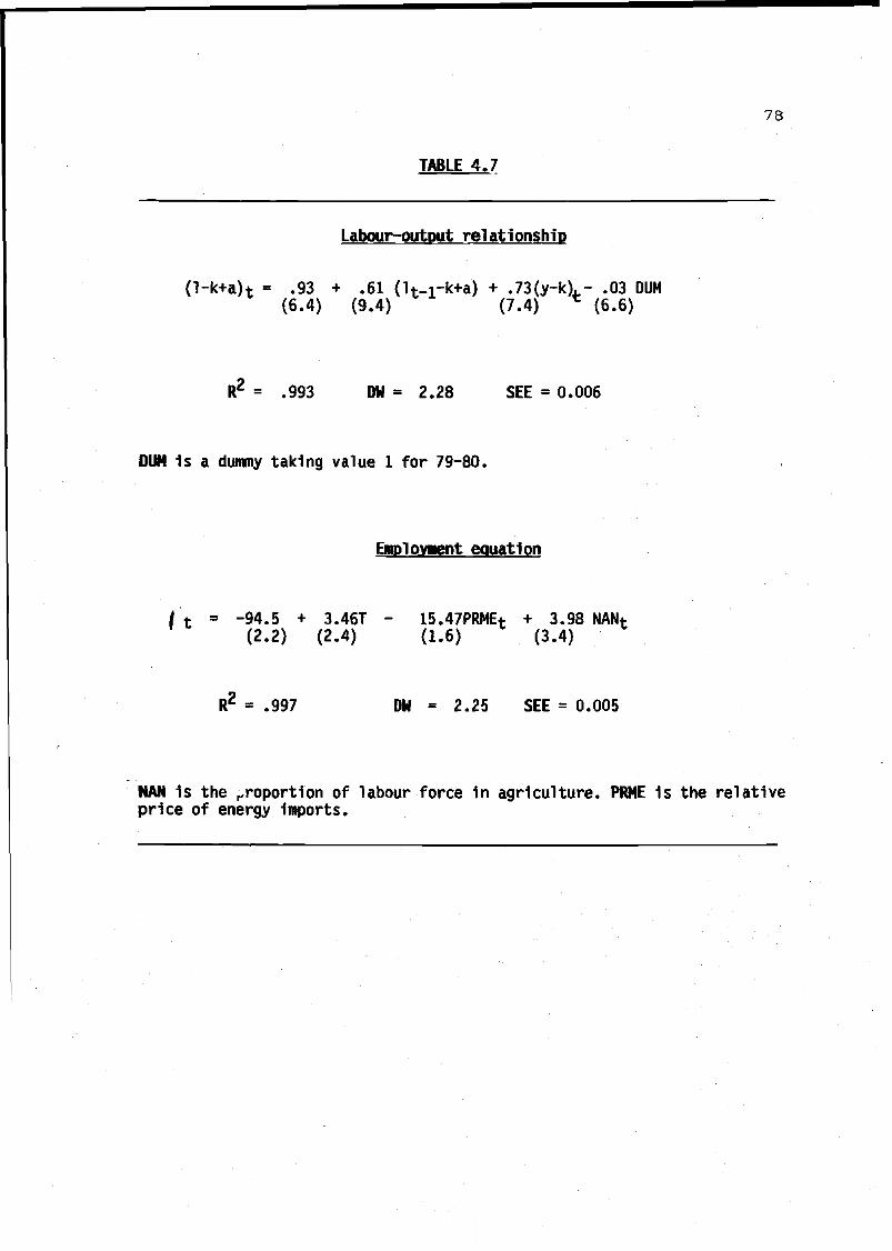
78

TABLE 4.7

Labour-output relationship

(l-k+a)t = .93 + .61 Ot-i-k+a) + .73(y-k),- .03 DUM(6.4) (9.4) (7.4) * (6.6)

R2 = .993 DW - 2.28 SEE = 0.006

DUM 1s a dummy taking value 1 for 79-80.

Employment equation

ft " -94.5 + 3.46T - 15.47PRMEt + 3.98 NANt(2.2) (2.4) (1.6) (3.4)

R2 * .997 DW = 2.25 SEE = 0.005

NAN 1s the roportton of labour force in agriculture. PRME 1s the relativeprice of energy imports.

TABLE 4.8

79

19651966196719681969197019711972

19731974197519761977197819791980

1981198219831984

1985

L

12156.8

12291.112367.012426.012504.2

12501.312599.012825.013053.513222.113000.312761.512755.812604.611896.011367.011172.011061.010984.010668.010571.0

Values of LT. LK. LP(in thousands)

LS12340.812397.1

12492.012552.112622.7

12633.812791.013103.313357.013575.113514.813412.613504.313595.613101.312858.113045.013206.013353.4

13437.013542.0

and LS

LP12459.412597.112868.412764.2

12813.0

12948.612916.012910.313053.513329.513417.613279.613092.112842.1

12359.312017.911785.811575.211358.311134.010979.4

LK12424.6

12577.912478.312603.7

12882.4

12897.912865.813496.213943.713730.313171.1

13115.413184.012779.212083.311458.711255.211237.2

11073.710755.510586.8

80

TABLE 4.9

196519661967

1968196919701971197219731974

197519761977

19781979198019811982198319841985

Frictional

PK0.2960.2190.4860.364

0.1610.184

0.3120.0550.0210.1320.5300.4760.3680.504

0.6610.8330.7970.7030.7020.7760.807

unemployment

PC0.2470.198

0.0620.154

0.2290.144

0.2470.6580.7600.6290.2660.307

0.4550.4290.3000.1530.1950.2910.2960.2240.193

and regime

PRI0.4580.582

0.4520.4820.6100.671

0.4420.2870.2190.2400.2030.2160.1770.0670.0390.014

0.0090.0060.0010.0000.000

proportions

RHO64.65867.39366.70768.16265.34062.475

59.80955.94854.17252.77037.20835.18930.44732.51035.027

35.49330.59729.734

33.99435.92539.242

SURE0.0170.0160.0160.0160.0170.017

0.0180.0190.0200.0200.0290.0310.0350.0330.0310.0300.0350.0360.0320.0300.028

81

ANNEX 1

In this Annex we report an estimate of a Marshallian labourdemand equation, corresponding to an oligopolistic representativefirm which faces an isoelastic demand function for its product (seeLayard and Nickell (1985)). In this framework, the specification ofthe labour demand function is as follows:

L = L (K, «(l+TiJ/P, duk, A)

where constant returns to scale and labour augmenting technologicalprogress imply the following restrictions on the elasticities/denoted by e, respectively:

eLK - 1

eiA • ULW! - 1

Both restrictions are easily accepted by the data.

The estimated equation is:

H - H-l = --04 ' •151t-l + -15*kt - .18(w + tj-pJt + .34 dukt +(2.4) (11.7) (3.2) (3.4)

+ .15 dukt-i + .20*at(3.0). t X *

SEE .011 DW = 1.8 LM(4) = 4.2

t - ratios in parenthesis* denotes restricted coefficient.k : X2(l) = 1.0a : X2(l) =2.1

82

ANNEX 2

Employment function with "effective" labour supply

f\ * 91.7 - 16.5 PRMEt - 4.9 mmt - .71 brkt(7.3) (2.3) (3.1) (2.2)

LF = 1.36 LS - .60 rr(37.8) (10.3)

R2 = .999 DW = 2.15 SEE = 0.003

Estimation period: 1965-85

Estimation method: Non Linear Least Squares

Using the previous estimate of LF, we can decompose theunemploment rate U which appears 1n the wage equation (see Table 4.1)Into two components: an effective unemployment rate, Us (= 1- L/LF)and a disenfranchised unemployment rate, Uf(= U-Us). The interestingnull hypothesis to test is whether Uf is significant. The estimatedequation 1s similar to the previous one with the followingcoefficient estimates (t-rat1os) for the unemployment rates,-.88(6.7) for Uf and -1.33(4.8) for Us. An F-test to test theequality of both coefficients gives a value of 1.0 which is non-significant at 5% significance level. Therefore, we can reject boththe hypothesis that the disenfranchised unemployed workers do notexert downwards wage pressure, and that their pressure is smallerthan that of the other unemployed. However the point estimates showthat the effect of Uf is 40% smaller than that of Us, as we wouldexpect from a partial interpretation of the hysteresis effect.Further work on this Issue is in the research agenda.

83

FIGURE A-2

ACTUAL AND EFFECTIVE LABOUR SUPPLY14OOO

138ÜO-• LS

LF

136OO-•

1 34OO - •

13200-

130OO- -

1 28OO - -

126OO- -

124OO-•

122OO-•

/

12000-1965 1967 1969 1971 1973 1975 1977 1979

V1—

1981

///

1982 1985

84

19661967196819691970197119721973197419751976197719781979198019811982198319841985

APPENDIX (ANUAL FIGURES FOR

LAYER 1

dL/L A(LP/YP)/(LP/YP)

•110473E-01.617520E-02.477885E-02•628516E-02

-.231922E-03.781519E-02•179617E-01.177930E-01.129161E-01

-.167749E-01-.183688E-01-.446656E-03-.118534E-01-.562176E-01-.444687E-01-.171549E-01-.993555E-02-.696140E-02-.287691E-01-.909261E-02

-.480908E-01-.416665E-01--656462E-01-.621009E-01-.488290E-01-.481389E-01-.523806E-01-.523196E-01-.416635E-01-.392284E-01-.392897E-01-.412929E-01-.314753E-01-.436718E-01-.401654E-01-.445224E-01-.321401E-01-.353291E-01-.313790E-01-.364624E-01

LAYERS 1 TO 4)

AY/Y ;

.706975E-01

.430882E-01

.677193E-01

.894366E-01

.408048E-01

.495303E-01

.814039E-01

.785595E-01

.571728E-01

.109781E-01

.301142E-01

.329781E-01

.179562E-01

.186255E-02

.154469E-01

.444241E-02

.879192E-02

.210177E-01

.204549E-01

.199939E-01

RESIDUAL

-.115595E-01•475350E-02.270567E-02

-.210506E-01.779227E-02.642376E-02-.110616E-01-.844688E-02-.259314E-02.114753E-01--919335E-02.786814E-02.166563E-02-.144083E-01•.197502E-01.229250E-01.134126E-01.735002E-02.178451E-01.737586E-02

85

LAYER 2

1966196719681969197C197119721973-197419751976197719781979198019811982198319841985

¿Y/Y

.706975E-01

.430882E-01

.677193E-01

.894366E-01

.408048E-01

.495303E-01

.814039E-01

.785595E-01

.571728E-01

.109781E-01

.301142E-01

.329781E-01

.179562E-01

.186255E-02

.154469E-01

.444241E-02

.879192E-02

.210177E-01

.204549E-01

.199939E-01

PIK( A YD/YD).156768E-01.171217E-01.257632E-01.158872E-01.767050E-02.136355E-01.543742E-02.185958E-02.543489E-02

-.121862E-02.181154E-01.132847E-01.377830E-02.189420E-02.942929E-02.327783E-02.937185E-02.118206E-01.158844E-01.131917E-01

PIC( ¿YP/YP).123085E-01.411188E-02.947299E-02.161158E-01.901205E-02.118329E-01.360749E-01.485681E-01.430792E-01.126942E-01.927980E-02.128986E-01.548639E-02.190488E-02.200381E-02.513422E-02.429544E-02.509760E-02.268814E-02.452774E-02

PIC(fc> YS/YS).322149E-01.232447E-01.363384E-01.440178E-01.350844E-01.281042E-01.232538E-01.165484E-01.145140E-01.736479E-02.714784E-02.889029E-02. 265469E-02.297506E-03.313659E-03.538809E-03.265788E-03.583204E-04.101453E-04.236199E-05

RESIDUAL-.104973E-01.139007E-02.385522E-02

-.134158E-01.109622E-01.404234E-02.166378E-01

-.115833E-01.585528E-02.786225E-02.442883E-02.209545E-02.603685E-02.223403E-02.369811E-02.450845E-02.514116E-02.404113E-02.187217E-02.227204E-02

86

LAYER 3.1

19661967196819691970197119721973197419751976197719781979198019811982198319841985

Sc(Ac/c)

.469068E-01

.404804E-01

.413229E-01

.477646E-01

.279424E-01

.330662E-01

.558835E-01

.541482E-01

.332918E-01

.160031E-01

.317732E-01

.173952E-01

.916376E-02

.809670E-02

.892995E-02-.612829E-02.452639E-02.495608E-02

-.775724E-02.100125E-01

SjíóI/I)

.292750E-01

.482914E-03

.163697E-01

.406228E-01-.318111E-02-.458045E-02.362060E-01.299514E-01.263229E-01

-.940611E-02-.353558E-02-.965014E-02-.142445E-01-.244723E-02.813366E-02

-.101870E-01-.667466E-02-.632325E-02-.647765E-02.787113E-02

S_(AG/G)G

.166739E-02

.215602E-02

.170588E-02

.366152E-02

.435842E-02

.391331E-02

.458539E-02

.539939E-02

.653441E-02

.430371E-02

.460109E-02

.364517E-02

.486095E-02

.392402E-02

.419870E-02

.143943E-02

.655943E-02

.489967E-02

.221950E-02

.386927E-02

¿(XD-MD)/YD

-.641734E-02-.788967E-02.113207E-01.653381E-02.124864E-01.113694E-01.227263E-02

-.224189E-02-.248653E-01-.131979E-01.520071E-02.247286E-01.772375E-02

-.670902E-02-.993757E-02.189904E-01.891981E-02.132962E-01.324896E-01

-.539991E-02

87

LAYER 3.2

19661967196819691970197119721973197419751976197719781979198019811982198319841985

AYP/YP.621257E-01.659544E-01.615914E-01.702946E-01•624541E-01.479283E-01.548160E-01.639134E-01•685423E-01.477044E-01.301942E-01.283419E-01.127813E-01•635321E-02.130730E-01.263778E-01.147507E-01.171995E-01.120053E-01.234279E-01

A K/K.348281E-01.314592E-01.333064E-01.501872E-01.526547E-01.414934E-01.592299E-01.727162E-01.734336E-01.568529E-01.450757E-01.390903E-01.320342E-01.232113E-01.229947E-01.227931E-01.163191E-01.871537E-02.442285E-02.110876E-01

£(YP/K)/(YP/K).263789E-01.334431E-01.273733E-01.191465E-01.930924E-02.617849E-02

-.416706E-02-.820608E-02-.455675E-02-.865628E-02-.1.42396E-01-. 103.4 41-E-01-.186553E-01-.164756E-01-.969871E-02.350478E-02

-.154330E-02.841082E-02.754909E-02.122050E-01

RESIDUAL.918728E-03.105209E-02.911705E-03.960909E-03.490175E-03.256367E-03

-.246815E-03-.596715E-03-.334618E-03-.492134E-03-.641860E-03-.404352E-03-.597609E-03-.382420E-03-.223019E-03.798851E-04-.251854E-04.733034E-04.333885E-04.135324E-03

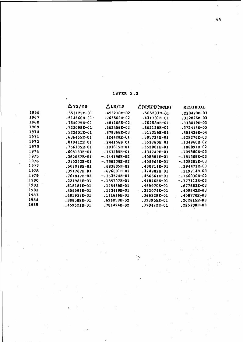
LAYER 3 .3

88

19661967196819691970197119721973197419751976197719781979198019811982198319841985

AYS/YS.553129E-01.514660E-01.754075E-01.722098E-01.522601E-01.636455E-01.810412E-01.756385E-01.605133E-01.362067E-01.330252E-01.502028E-01.394787E-01.764847E-02.224984E-01.618181E-01.459591E-01.481933E-01.388589E-01.459521E-01

ALS/LS

.456210E-02

.765502E-02

.481108E-02

.562456E-02

.879368E-03

.124428E-01

.244156E-01

.193615E-01

.163285E-01-.444196E-02-.756208E-02.683685E-02.676081E-02

-.363574E-01-.185707E-01.145435E-01.123419E-01.111616E-01.626058E-02.781424E-02

¿1(YP/LP)/ÍYP/II>).505203E-01.434781E-01.702584E-01.662128E-01.513356E-01.505734E-01.552760E-01.552081E-01.434749E-01.408301E-01.408965E-01.430714E-01.324982E-01.456661E-01.418462E-01.465970E-01.332074E-01.366229E-01.323955E-01.378422E-01

RESIDUAL.230479E-03.332826E-03.338019E-03.372418E-03.451429E-04.629276E-03.134960E-02. 106891E-02.709880E-03

-.181365E-03-.309263E-03

.294473E-03

.219714E-03-.166030E-02-.777H2E-03

.677682E-03

.409842E-03

.408770E-03

.202815E-03

.295708E-03

r 89

LAYER 4.1

19661967196819691970197119721973-9741975»1976-197719781979198019811982198319841985

A(LP/YP)/(LP/YP)

-.480908E-01-.416665E-01-.656462E-01-.621009E-01-.488290E-01-.481389E-01-.523806E-01-.523196E-01-.416635E-01-.392284E-01-.392897E-01-.412929E-01-.314753E-01-.436718E-01-.401654E-01-.445224E-01-.321401E-01-.353291E-01-.313790E-01-.364624E-01

TECH. PROGRESS

-.414311E-01-.435488E-01-.432348E-01-.411304E-01-.378093E-01-.337773E-01-.294729E-01-.252667E-01-.214616E-01-.182930E-01-.159286E-01-.144684E-01-.139448E-01-.223224E-01-.234982E-01-.253016E-01-.274945E-01-.297707E-01-.317567E-01-.330114E-01

RELATIVE PRICE

-.214523E-01-.237113E-01-.203447E-01-.225080E-01-.202942E-01-.215050E-01-.290921E-01-.311612E-01-.235166E-01-.243291E-01-.272599E-01-.263059E-01-.254052E-01-.222396E-01-.169044E-01-.125386E-01-.863751E-02-.536526E-02-.377473E-02-.409578E-02

RESIDUAL

.147927E-01

.255936E-01-.206662E-02.153756fi-02.927447E-02.714343E-02.618441E-02.410825E-02.331469E-02.339380E-02.389880E-02

-.518572E-03.787469E-02.890139E-03.237164E-03

-.668215E-02.399191E-02

-.193100E-03.415243E-02.644852E-03

' LAYER 4.2

19661967196819691970197119721972197419751976197719781979198019811982198319841985

¿1 (X-M)

-.351243E-01-.135928E-01.907733E-01-.109080E-02.932044E-01.114756

-.104549-.661900E-01-.667616E-01-.222470E-02-.158700E-03.130454.107733

-.451121E-01-.324125E-01.102032.183034E-01.827717E-01.138543-.175240E-01

WT

.185673

.102924

.236152

.221324

.196163

.114579

.171988

.244086

.773298E-01-.976143E-01.241554.106846.122261.109113.114760E-01.755171E-02-.249941E-01.364070E-01.176060.830309E-01

Y

-.175186-.107972-.166339-.220441-.102235-.123680-.201988-.189908-.145571-.268047E-01-.761046E-01-.837960E-01-.455644E-01-.452211E-02-.396434E-01-.108454E-01-.225670E-01-.534121E-01-.517186E-01-.493768E-01

RELATIVE PRICES

-.453357E-01-.506917B-01.568068E-01.502280E-01.206121E-01.378579E-02-.401056E-01-.356719E-01-.586759E-02.208179E-02.111533E-01

-.106808E-01-.457482E-01-.171123.693297E-01.134712.329014E-01.128077

-.587080E-01-.230483E-01

DUK

.000000

.535276E-01-.180625E-01-.528785E-01.000000.350378E-01-.860605E-01-.330469E-01.840697E-01.709410E-01-.359032E-01-.176244E-01.535276E-01.000000.182894E-01.000000-.182894E-01.182894E-01.000000.185227E-01

RESIDUAL

-.275173E-03-.264050E-02.285766E-01

-.532836E-01-.236157E-01.835140E-01.238774E-01

-.649496E-01-.375827E-01.514516E-01

-.713179E-01.117089-.219628E-01-.325403E-01-.154843E-01.298936E-01.128726E-01

-.359494E-01.364292E-01

-.580525B-01

NOMINAL SURPRISE

.000000-.874000E-02-.463600E-01.539600E-01.228000E-02.152000E-02.277400E-01.133000B-01

-.391400E-01-.228000E-02-.695400E-01.186200E-01.452200E-01.539600E-01

-.763800E-01-.592800E-01.383800E-01

-.106400E-01. 364800E-01.114000E-01

COo

91

LIST OF VARIABLES AND DATA SOURCES

Variables:

A: Labour augmenting technical progress (own estimates).

DUK: Capacity utilization in industry (Survey of Entrepreneur'sOpinions, BE).

D: A truncated trend taking 0 value for 1964-77, T-14 for1978-85.

DUM: A dummy variable taking 1 value for 1979-80, 0 elsewhere.

KLS: Capital/labour supply ratio. Capital series (see Balges etal. (1986)) estimates) divided by labour supply (thousands)(INE.EPA).

L : Number of employed (in thousands) (EPA).

M: Real imports (in thousands of 1970 pts.) Exports includingtourism expenditures (INE,CN).

MO : Real oil imports (in Thousand 1970 pts.). Oil imports (BE)divided by the oil imports unit value (MECO).

MNO: Real non-oil imports (in thousands 1970 pts.). Non-oilimports (BE) divided by the implicit non-oil imports de-flator obtained from the imports deflator and the oilimports deflator.

MM : An index of mismatch. Sum of absolute changes in theproportion of total employees in each sector relative tototal employees (GTE and EPA).

MAN : Proportion of agricultural labor force (GTE and EPA).

PIP: Relative price of investment. Gross fixed investment de-flator divided by GDP deflator.

PREL: Ratio of CPI (INE) to GDP deflator (market prices) minusindirect taxes (INE.CN).

PRME: Relative price of oil imports. Oil imports deflator dividedby GDP deflator.

92

PRMC: Relative price of consumption imports goods. Consumptionimportables unit value divided by GDP deflator.

PRX: Relative price of exports (relative to wold) . Spanishexports unit value (MECO) divided by world exports unitvalue (IPS) times the appropiate exchange rate.

PRXI: Relative price of exports (relative to industrialcountries.). Spanish exports unit value (MECO) divided byindustrial countries' unit value (IPS) times de appropriateexchange rate.

t2 : Income taxes. Total income tax colection (IGAE) over GDP(INE, CN).

t3: Indirect tax rate. Total excise collections divided bynominal private consumption (IGAE and INE).

U: Unemployment rate (INE-EPA).

W(l+ti): Total real labour cost (monthly). W: Real wage (obtainedfrom total monthly labour share on GDP divided by employ-ment (INECN). (1+ti): Total effective rate of employer'scontributions to the Social Security (own estimates).

HPI: W(l+ti) divided by PIP

WT: Real world trade. World imports in $ (IPS) divided by worldImports unit prices in $ (IPS).

X: Real exports (in thousands of 1970 pts.) Exports excludingtourism expenditures (INE,CN).

Y: Real GDP (in thousands 1970 pts.). (INE.CN). (Intechnological equations we use at factor costs. In nationalaccounts identities we convert it into market prices).

93

Abrev1at1ons for sources

BE Boletín Estadístico (Bank of Spain)

CN Contabilidad Nacional

EPA Encuesta de Población Activa

GTE Grupo de Trabajo del Ministerio de Economía y Hacienda

IPS International Financial Statistics (IMF)

MECO Ministerio de Comercio

IGAE Intervención General de la Administración del Estado

INE Instituto Nacional de Industria

94

REFERENCES

ANDRES, J. NOLINAS, C. Y TAGUAS, 0. (1987): "Una función de ConsumoPrivado para la Economía Española". D.G. de Planificación. M^ deEconomía y Hacienda.

BAIGES, J. MOLINAS, C. Y SEBASTIAN, N. (1987): "La Economía española1964-85. Datos, fuentes y análisis". Instituto de EstudiosFiscales.

BEAN, Ch. (1981): "An Econometric Model of Manufacturing Investmentin the U.K.". Economic Journal vol. 91. 106-121.

BEAN, C. and GAVOSTO, A.(1987): "A discussion of British Unemploymentcombining traditional concepts and disequilibrium economics: apreliminary report", CLE Working Paper No.976.

ilLS, M. (1985): "Emperlcal Structure Evidence on Wages, Prices andemployment in the U.S.". Journal of Political Economy

BONILLA, J.M. (1978): "Fundones de Importación y Exportación para laeconomía española", Estudios Económicos. No. 14,, Banco deEspaña.

DOLADO, J.J.; MALO DE MOLINA, J.L. and ZABALZA, A.(1986): "SpanishIndustrial Unemployment: Some Explanatory Factors", EconómicaVol.53, No. 210.

ENGLE, R.F. y GRANGER, C.W.J. (1987): "Co-integration and errorcorrection: representation, estimation, and testing". Econome-trica. 55. ns 2, pg. 251-276.

FELDSTEIN, M. (1982): "Inflation, Tax Rules and Investment: SomeEconometric Evidence". Econometrica Vol. 50, n2 4 pg 825-862.

95

FERNANDEZ, J.I. and SEBASTIAN, M. (1988): Funciones de Importación yExportación para la Economía Española. Mimeo.

GAGEY, F., LAMBERT, J. and OTTENUAELTER, B (1987): A DisequilibriumEstimation of the French Labour Market. A Preliminary Report.Mimeo.

HENCHY, D., PAGAN, A. and SARGAN, J.D. (1984): "DynamicSpecification" en Griliches, A, and M. Intrilligator eds.,Handbook of Ecomometrics. North Holland

LAMBERT, P. (1987): "Disequilibrium Macro Models", Cambridge Univer-sity Press. Cambridge.

LAYARD, R. and NICKELL, s. (1985): "Unemployment in Britain". Econó-mica vol. 53 pg.

MAULEON, I. (1985): "Análisis eco: ométrico de las importacionesespañolas". Documento Interno Servicio de Estudios. Banco deEspaña.

MAULEON, I. (1986): "Una función de exportación para la economíaespañola", Investigaciones Económicas, vol. X, No. 2, pág.357-378.

MOLINAS, C.; SEBASTIAN, M. and ZABALZA, A. (1987): "EuropeanUnemployment Program: preliminary results on SpanishUnemployment". Mimeo.

NICKELL, S. (1986): "The Supply Side and Macroeconomic Modelling".Mimeo.

ROTEMBERG, a. and SALONER, G. (1986): "A Supergame - TheoreticalModel of Price Wars during booms". American Economic Review

96

SNEESENS, H. (1987): "Investment and the Inflation UnemploymentTrade-off in a macroeconomic Rationing Model with MonopolisticCompetition". European Economic Review, pg 781-808.

SNEESSENS, H.R. and DREZE, J.H. (1986): "A Discussion of BelgianUnemployment Combining Traditional Concepts and DisequilibriumEconomics", Económica. Vol. 53, No. 210.

SNEESSENS, H.R. and DREZE, J.H. (1987): "Report on the Project onEuropean Unemployment", CORE, manuscript.

UNGERN-STERNBERG, T. (1981): "Inflation and Savings: InternationalEvidence on inflation-induced income losses". Economic Journal.Vol.91, pg. 961-976.