&AC-PUB-849 January 1971

ANOTHER BOUND ON THE ABSORPTIVE PART

OF ELASTIC SCATTERING AMPLITUDES*

R. Savit, R. Blankenbecler

Stanford Linear Accelerator Center Stanford Univers.ity, Stanford, California 94305

M. B, Einhorn

Lawrence Radiation Laboratory Berkeley, California 94720

ABSTRACT

Using Lagrange multipliers for inequality constraints, an upper

bound on the absorptive part of elastic scattering amplitudes is derived

assuming unitarity, a fixed total and elastic cross section, and the

condition that the partial waves decrease monotonically with increasing

angular momentum. Numerical results are given,

(Submitted to J. Math. Phys.)

* Work supported in part by the U, S. Atomic Energy Commission.

1. INTRODUCTION

Consider the elastic scattering of equal mass particles of spin zero, Given

the total cross section and the elastic cross section, as well as the unitarity

requirement on the partial wave amplitudes, how large can the absorptive part

of the elastic scattering amplitude become at any given scattering angle? This

problem has been solved by Singh and RoyI and the maximum value has been

compared with experimental differential cross sections at high energies and for

small scattering angles on the basis of several further assumptions : (1) At high

energies, the equal mass assumption can be relaxed. (2) The unpolarized

differential cross sections are independent of the spin of the external particles

and, hence, the spin zero bound applies. (3) The amplitude, in the region of

the diffraction peak, is purely imaginary. The comparison’ with experimental

data is rather good for small angles, but for larger angles the data falls far

below the calculated bound.

The distribution of partial Wave amplitudes which achieves this bound looks

very much like a Fresnel zone plate, carefully constructed to maximize the scat-

tering in the given direction., The distribution is illustrated as the shaded region

of Fig0 1, the details of which will be explained later. The larger the angle, the

more zones are required. More conventional models of matter would have a

central core surrounded perhaps by successively less absorptive regions. A

particularly simple way to implement this intuition is to require the imaginary

parts of the partial wave amplitudes to decrease monotonically with increasing

angular momentum. 2 This is not unreasonable for energies above resonances.

Adding this assumption to those given above should yield a better bound at larger

angles, precisely where the preceding one fails. It is to the solution of this

problem that this paper is devoted. The approach used in the construction of the

-2-

solution is the method of Lagrange multipliers generalized to include inequality

constraints O 3

In Section 2, the mathematical problem is formulated and solved exactly.

In Section 3, the same problem is simplified by approximating the discrete

partial wave series by a continuum and by assuming the scattering angle is small.

Section 4 compares the improved bound with experimental data and interpretes

the results., Finally, in Section 5, we summarize our conclusions. In an appendix,

a number of sums are tabulated.

-3-

2. MATHEMATICAL DETAILS

The mathematical statement of the problem is as follows4: Maximize

A = c(Za+l) anPa

given the total cross section

k2 Ao=zUT= c w+11 aQ

the elastic cross section

c k2 =- el 4A uel = C(2Ptl) (a: + ri)

and unitarity

2 2.0 ua = at-at -ra - d=O,l,2, 00.

In addition, we require that the partial waves decrease monotonically, i. e.,

(1)

However, thinking of the requirements of statistics as well as of most dynamical

models, one would like to impose this requirement separately on the even and

odd partial waves, i.e.

Fortunately, this is a minor complication. To avoid notational confusion, we

solve the problem first assuming (1) and then state the result assuming (2) o From

a mathematical point of view, these requirements are interesting since they

impose a relation between neighboring partial waves, unlike those examples

discussed in EB.

To this end, we introduce the auxiliary function

-4-

where, on the basis of the theorem3 that the multipliers are the rate of change

of the maximum with respect to the constraint, we anticipate that

OCa!<l and a>0 o

Of course, hQ 2 0 and UQ 2 0 for all I. Varying with respect to rQ, we find

- = (2Q+l) [- $ - 2AQ] rQ =‘O . s”; This implies rQ=OO Also,

- = (2Q4.1) [PQ - o! i; aQ - a + AQ(l - 2aQ) + (wp- w,$(Ze+l) 1 = 0 . (4)

For convenience, we have defined wml =O, First, we must find what are the

,

necessary conditions on a local maximum. The most general form for a local

maximum under these assumptions is

, x=ll=l=OOO = a NO ’ aNo+l 2ooo ia

Ll =aLI+I=eO.=aLI+N1>

aL1+N1+l > *. 0 > aL2=aL2+p 0 l “aL 2 +N 2’ ;tL2+N2+1

In words, the solution is a series of plateaus, on which at least two partial waves

have the same value, and regions where successive partial waves are strictly

decreasing. Our problem is to determine where the transition points and jumps

occur as well as the values of a Q’ As in EB, we define three partitions of the

partial waves

Bl ={QlaQ = l}

I ={QlO < aQ < I}

Bo={Q]aQ=O~ ,,

A priori, Bl, I, or B. could be empty. It follows from our variational equations

(4) that, in Bl,

in I,

AQ=PQ-a++ “Q-“Q-l > o 2Q+l , (9

AQ=o, “Q-l- Urn 9

2Q+l =?@-“‘a ’

and in Bo,

hQ =a! 1 0 0

(9

tw Let us first determine the properties of each of the transition points where aQ

actually decreases,

1. aN ’ aNo+l implies 0 0 NO

=0, hence, from (5a)

UN04 hNo=PNo-(Y-$ -

2No+l ’ ’ ’

consequently,

1 pNO-a-z2

WNO-l 2No+l ’ ’ ’

In particular, this means that a P -a! 2 1 so, as in the case 3 NO

without monotonicity, Bl is empty if a( l-a) < 1.

2, In I, if, for any I, one has aQ 1 > aQ > aQ+l) then w Q-l=“m=OO

Hence, from (b)

aQ = a(P,-o) 0

Of course, by the definition of I, one must have 1 > a(PQ-cr) > 0.

-6-

3, aLN-+ ’ aLN = 0 implies wL -l=O. So, from (5c), N

ALN=a-PLN-

wLN -20, 2LN+1

In particular, this means that Q! 2 P LN ’

Now we come to the heart of the problem, how to determine the plateaus of

constancy. The three points immediately above suggest that the multipliers a

and Q! determine where B 1 stops and the value of largest nonzero partial wave I , amplitude, just as in the case without the monotonicity requirement. In I, we

. shall find that the transition poini% are determined independently of a and a!. In

other words, rT and eel determine the size of the core (Bl) and the value of

the largest contributing partial wave (Bo) D However, in the intermediate region

(I), the shape of the distribution is determined solely by the requirement that the

strength of the partial wave amplitudes should be monotonically decreasing. To

see this, consider any particular plateau

aLj-l ’ “L. = ” ’ = “L.+N. ’ ‘Lj+Nj+l ’ 3 3 3

We know that oL =O. Using the difference equation (5b), one can then solve j -I

for Lj+n

-WLj-t-n =c (ZQ+l) (PQ-cx-2)

L. 3

n=O N ,0.0, .O 3

-7-

^.

using a~ +N =O, we find j j

0 =

L .+N. J J

c @+I) L.

J

(PQ-o->) D

It is convenient at this point to define a weighted average of the Legendre poly-

nomials

$PQ>M 5 &!+I) PQ/$ &+l) l

Q=M Q=M

Notice that d > PQ N = PN and that

&PQ+c>M = $PQ& + c for any constant c.

We have found in Eq. (4) that

aL =a j

L +N< ‘Q$, - a jj j

Thus the value of the partial wave amplitude is related to the weighted average

of the Legendre polynomials across the plateau. The requirement a L. > 0 implies

Lj+NJ<‘Q’Lj ’ QI ’ ” 3

Therefore, a! determines the largest nonzero partial wave.,

Inserting this solution for aL into the equation for oL +n, we have j j

Lj+n

Note that this can also be written as

The condition oL +n > 0 therefore implies j

L+N<'Q)L ' L +n<'Q>, for n=O, 0 D., N. jj j j j J

or

<P > <p > Lj+Nj Q Lj+Nj-n ’ Lj-i-Nj Q L. for n=O, . . *, N. 3 J

It can be shown that the conditions that wL I=0 and aL I > a j-

L imply

‘L -1’L +N<‘Q)L j- *

, while the conditions w j jj j L+N=OandaL

j j j ’ a;+N+l’ UnPlY

<,.j j

L +N<pm>L jj j

’ ‘Lj+Nj+l ’

We may summarize all of these inequalities as

P L -1’ L +N”Q’L ’ ‘L +N +1 j 43 j jj

(9

and

L +N('Q)L +m ’ L +N”Q& ’ JJ +n<‘Q>L n,m=O,l, ..,*, N jj j jj j j j

j (8b)

As the derivation shows, either of the two inequalities in (8b) implies the other D

Notice that all reference to 01 and a have disappeared so that the plateau interval

[ 1 Lj, Lj+Nj may be determined solely by properties of the Legendre polynomials.

Since successive plateaus must be monotonically decreasing, the condition

L +NCpQ>L > 01 is significant only for the last interval, i.e., only for determining jj j

Bo. Thus we may determine all possible plateau intervals independently of the

multipliers CY and a. Since for a maximum (Y is greater than zero, we may

‘restrict our determination to those for which L “+,<pQ>, > 0. jj j

-Q-

We have now completely characterized the necessary conditions on a local

maximum. In summary, the last value NO in B1 must satisfy a(PN -a) 2 1. If 0

ai-1 > at > al+l, then 1 > a1 =a(P,-o) > 0. The plateau interval must satisfy the

sets of inequalities expressed by Eqs. (8a) and (8b). On a plateau,

1 aL=a ( L +N<‘~>L -ol> ’ O”

j jj j Finally, the first partial wave LN for which

at vanishes must satisfy Q! 2 P LN’

To determine the local maximum, one must

determine the sufficiency of these many conditions. We have not been able to

show that these conditions uniquely determine the local maximum; indeed, we

suspect that one can probably find some angles for which the local maximum

is not unique. 5 Given any given scattering angle, one can use the inequalities

to determine the plateau intervals. Then, given uT and o,,, one can try to

determine CY and a to satisfy the equality constraints. In practice, it is easier

and faster to choose Q! and a and to then calculate the corresponding c T and

f el”

It is a simple matter now to solve the problem where the monotonicity re-

quirement is applied to the even and odd partial waves separately (Eq. (2)) 0 The

general form of the local maximum is

x even

2M0 > ‘2Mo+2’ l l ’ ’ “2K1 = “2K1+2 = ’ ’ l = “2Kl+2M1’

a2K1+2M1+2> . ..> a2KM=O=0=.0.

xodd 2No+1 ’ a2No+3 ’ 0 0 0 > a2L,+1=a2LI+3=’ ’ a =a2Ll+2Nl+l’

Correspondingly, we are led to define weighted averages over the even and odd

partial waves separately

N

&‘&&,I s c (4n+1) ‘sn (~+11 ’ n=M

N N 2N+1(‘Q)2M+l= x (4n+3) ‘.-&+I -. I= W+3) n=M n=M

The preceding solution then becomes the correct’solution to this problem if one

everywhere treats the even and odd partial waves separately. For example,

for the even case, the last value in B1 must satisfy a(P2M -a) > 1. The plateau

1 0

must .satisfy

‘2K j -2 ’ 2K +2M’pQ)2K

j j j ’ ‘2K +2M +2

j j

<p > 2Kj+2Mj”Q??Kj+2M ’ 2Kj+2Mj <P > Q 2Kj ’ 2Kj+2n Q 2Kj m,n=O,l, oOO, M. J

On the plateau, we find

Finally, the first partial wave which vanishes satisfies CY 2 P2K 0 Corresponding M

statements hold for the odd integers. In an appendix, we record the values for a

number of the sums and averages,

3. CONTINUUM APPROXIMATION

It is slightly more convenient in numerical applications to approximate Q by

a continuous variable since many partial waves contribute in general, and to

assume the scattering angle is s\mall. This approximation also makes it possible

to carry the solution further analytically and clarifies the result. Since one of

our purposes here is to illustrate a somewhat unfamiliar mathematical method,

we will solve the problem again in this approximation. Using the standard

replacement of the Legendre function by a Bessel function, the auxiliary function,

g, of the last section becomes

CD 2sin2 p=

s 0 xdx Jo(x) a(x) + CY

00 8a ‘TT - f 1 o xdx a(x) ’ IA2 pxdx a2(x) + O”xdx A(x) u(x) O” + 2a 7i5i~el-~o I I-

0 30 dx w(x) zJ$,

where

A2 s -t=4K2 sini! f , x N (2Q+l) sin $, O(x) = 2 Sin2 f wQ o

(For simplicity we have set rQ=O at the outset.) One consequence of replacing

the Legendre polynomials by Bessel functions has been to shift the dependence

on the momentum transfer to the boundary conditions. (Compare Eq. (3) 0) It

is important to remember that this approximation is best for small angles and

when many partial waves contribute to the sums. Notice that the monotonicity

Eq. (1) naturally translates into a negativity condition on the slope of the partial

wave amplitude. One could, of course, also generalize the monotonicity condition

separately applied to the even and odd partial waves by defining partial wave

amplitudes of even and odd signature, but for simplicity, we will ignore this

alternative. We will also assume that a(x) is a continuous function, so the most

- 12 -

general behavior possible has regions where a(x) is strictly decreasing separated

by regions of constant a(x) e

Formally, 9 is a function of a(x) and its first derivative da/dx; thus the

maximum satisfies the usual Euler-Lagrange equations. One finds

Jo(x) - a! - +$Q + h(l-2a(x))Si 2 = 0 (9)

As before, we label the three partitions of the solution B1, I, and Bo. The obvious

analogues of Eqs. (5a-c) are as follows:

B1: h(x) = Jo(x) - Q! - ; + ; 2 2 0

I: A(x) =o -1 dw ---& = Jo(x)-“-? (lob)

Bo: h(x)=a!- J,(x) -;g -0 . -. t w

On any interval, yi 5 x 5 xi+1 , on which a(x) is strictly decreasing, w(x) = 0 and

hence, dw/dx=O. Therefore,

a(x) = a(JO(x) - a) (11)

Continuity of a(x) then implies that

1 = at Jo(yo) - ~9 (12)

where y. is the largest value of x in B1 and that

0 = Jo(xn) - Q! , (13)

where xN is the smallest. value in ,Bo. Thus, the equality multipliers a and oc

determine the sets B1 and Bo. Of course, if l$ a( l-o), then B1 is empty,

Let us further explore the intervals, xi 5 x S yi, in I, on which a(x) is

constant, These are surrounded by intervals on which a(x) is strictly decreasing

- 13 - *

and, by Eq. (11) above, a(x) =a(J,(x) -a) on the surrounding intervals. However,

since a(xi) = a(y$ , continuity of a(x) then implies Jo(xi) = Jo&$ D It follows from

(lob) that w(x) is continuous in I and, since w vanishes on the surrounding intervals,

we have o(xi) = o(yi) = 0. Inside the plateau interval

do= dx x

3 1 = x J (x.) - Jo(x)

LO 1

Using w(xi)=O this may be easily integrated to obtain w(x). The condition w(yi)=O

then leads to

Jo(xi) = i i y<Jok ’

where, as in the previous section, we define the weighted average

,(Jo>, =

(See the Appendix for the explicit evaluation.) In summary, the end points of the

plateau interval satisfy

Jo(xi) i i = y< Jo>x = Jo(yi) (149

which may be compared to Eq. (Sa) for the discrete case. One may further

exploit the condition w(x) 2 0 inside the interval to obtain the analogue of Eq. (8b),

y<Jo>y 1 y< Jg>, L ,CJo>, ; for Xi’ X9 Y 5 Yi 0 w-8 i i i i

One can show, however, that these inequalities in fact follow from (14a), provided

that the plateau interval extends over only one cycle of J,(x). This makes finding

the plateau intervals easier in the continuous case than in the discrete case. And,

as before, the determination of the possible intervals do not involve a and a.

Given the multipliers a and ca, the necessary conditions given above are

also sufficient to determine to solution. These multipliers, in turn, are to be

determined from the equality constraints

A2 12 XN E”T=‘ZY(,+ I- xdx a(x)

YO

A2 8a uel

=+y;+ J XN xdx a2(x)

YO

where

atJO - a) yi5 xLxi+l a(x) =

atJotQ - 0~) xi5 XLY. 1

(15)

and, if B.,, is empty, yo=O, whereas, if B1 is not empty, 1 =a(Jo(yo) - ar) . In any

case, x N satisfies a! = Jo(xN) . A typical solutions is indicated in Fig. 1, where

the dashed curve is a(Jo(x) - 01) and the solid curve is the solution a(x) 0 The

shaded regions indicate the partial wave amplitudes in the problem without the

monotonicity constraint, described in the Introduction.

It is interesting to compare the expressions for the end of B1 and the start

ofB : 0 Jo(yO) = Q! + i and Jo(xN) = 01 0

As a becomes large, Jo(yO) N Jo(xd ., Since both these points must lie on falling

part of the curve a(x), one has y0 = xN as a gets large. Thus the ratio uel/oT

On the other hand, if a is smaller than (l-a) -1

approaches unity as a gets large. ,

then BI is empty and one expects a small value of the ratio ael/uTO

Given values of oT and gel from experimental data, one can determine a and

Q! and, subsequently, the maximum value of the absorptive part of the scattering

amplitude may be computed. We now turn to the numerical computations.

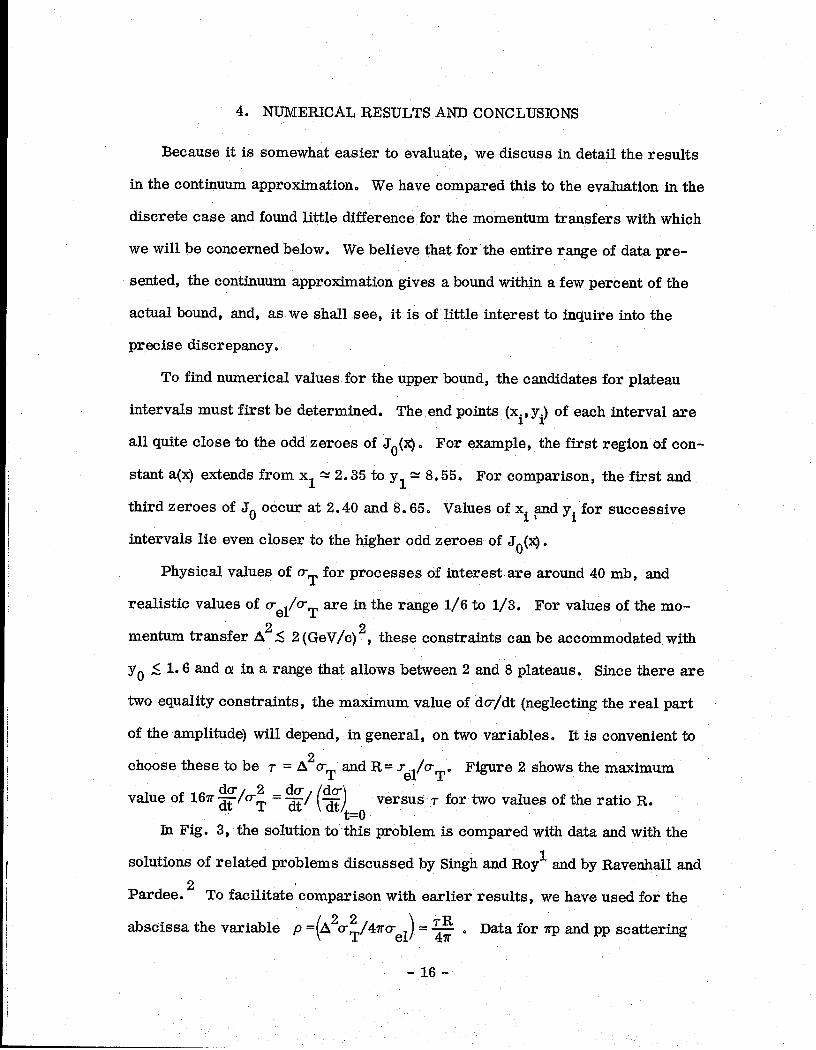
4. NUMERICAL RESULTS AND CONCLUSIONS

Because it is somewhat easier to evaluate, we discuss in detail the results

in the continuum approximation. We have compared this to the evaluation in the

discrete case and found little difference for the momentum transfers with which

we will be concerned below. We believe that for the entire range of data pre-

sented, the continuum approximation gives a bound within a few percent of the

actual bound, and, as we shall see, it is of little interest to inquire into the

precise discrepancy.

To find numerical values for the upper bound, the candidates for plateau

intervals must first be determined. The end points (xi, yi) of each interval are

all quite close to the odd zeroes of J,(x) 0 For example, the first region of con-

stant a(x) extends from x1 N 2.35 to y 1 2 8.55. For comparison, the first and

third zeroes of Jo occur at 2.40 and 8.65. Values of xi Fd yi for successive

intervals lie even closer to the higher odd zeroes of Jo(x).

Physical values of a;r for processes of interest are around 40 mb, and

realistic values of o el /oT are in the range l/6 to l/3. For values of the mo-

mentum transfer A2 ;S 2 ( GeV/c)2 , these constraints can be accommodated with

YO s 1.6 and a! in a range that allows between 2 and 8 plateaus. Since there are

two equality constraints, the maximum value of dcr/dt (neglecting the real part

of the amplitude) will depend, in general, on two variables. It is convenient to

choose these to be T = A2uT and R= rel/uTO Figure 2 shows the maximum

value of 167r g/u: = g/ ($) versus T for two values of the ratio R. t=o

In Fig. 3, the solution to’ this problem is compared with data and with the

solutions of related problems discussed by Singh and Roy’ and by Ravenhall and

Pardee. 2 To facilitate’comparison with earlier results, we have used for the

abscissa the variable p = A$~/4nuel ( > = s ,, Data for np and pp scattering

- 16 -

are indicated. 6 Curve A is the upper bound derived by Singh and Roy in the

absence of monotonicity constraints. Curve B is the bound given by Ravenhall

and Pardee for essentially the same problem as we have discussed. 7 The curves

C and C’ are the same bounds appearing in Fig. 2, only here plotted as a function

of p rather than of 7. Notice that in Fig. 2 C’ lies below C, while in Fig. 3

C’ lies above C over most of its range.

Inasmuch as the variable p has been ascribed some significance, 132 let us

comment on this variable. Suppose B1 were empty, so that yo=O. Then since

a(x)/a is independent of a for all x, the ratio

.X 1 A/A0 = ’

N xdx Jo@) a(x)

J XN

0 xdx a(x)

is independent of a and depends only on Q! 0 I However, setting yo=O in Eqs. (15)

and (16)) one sees that Q is determined by the ratio

Therefore, if Bl is empty, A/A0 is a function of p only, a property which has

been called “universality”. 192 This result is independent of the monotonicity

assumption. However, the actual values-for the experimental data usually require

that Bl g be empty. Thus, in general, the upper bound derived here will depend

on R as well as on p. Jn fact, one can show that

where the differentiation is performed for fixed p 0 While this is zero when Bl

is empty, it is not zero in general.

- 17 -

Comparing our upper bound with the data, we see that the addition of the

monotonicity requirement has significantly improved the bound of Singh and Roy;’

however, it still approximates the data only for a very small range of p. Already

at p= 10, the bound exceeds the data by a factor of 2; for typical values of u T and ~~1, this corresponds roughly to A2 s 0.3 (GeV/c) 2.

!

I - 18 - \

5. SUMMARY

One could have hoped that with such general considerations as crude unitarity

(uQ 10)) and the values of the total and elastic cross sections, the shape of the

diffraction peak might have been understood. Even assuming the real part of the

scattering amplitude is negligible, we found that only for very small values of the I

momentum transfer does the bound approximate the data, An exponential fit to

the data is a good approximation far beyond values of t for which our bound is

relevant.

One should note that the values of the. aQ which realize the maximum at a

particular angle depends on that angle. The upper bound plotted in our graphs

is not a reflection of any one set of partial wave amplitudes, but rather, as the

angle changes, the values of the aQ also change. Thus, for example, the area

under the upper bound could be much larger than ~~1, and this turns out to be the

case.

We conclude that, if the shape of diffraction peaks is to be understood, it is

not on the basis of the naive considerations discussed here. There is probably

a deep dynamical reason both for the small real part (if, indeed, it is small for

all t) and for the rapid decrease of the differential cross section with momentum

transfer.

ACKNOWLEDGEMENTS

Most of this work was performed while one of us (MBE) was still at SLAC.

We would like to thank Mr. Peete Baer of the SLAC Computer Center for illus-

trating the efficiency of the APL by finding the plateau intervals in the discrete

case. We also wish to acknowledge interesting conversations with Dr. S. Nussinov

concerning the statement of this problem.

- 19 -

APPENDIX APPENDIX

L

c pQ+1) PQ = P;L+l$ Pi

Q=O

L

c pQ+1) PQ = P;L+l$ Pi

Q=O

fi th+‘) th+‘) ‘Zn = ‘&+I ‘Zn = ‘&+I E (4n+l) (4n+l) = (N+l) (2N+l) = (N+l) (2N+l)

n=O n=O n=O n=O

N N N N

c c @nt-3) P5an+l @nt-3) P5an+l = ‘iiN+ = ‘iiN+ c c (4n+3) =(N+l) (2N+3) (4n+3) =(N+l) (2N+3)

n=O n=O n=O n=O

Hence Hence

P; = -& PQ(Z)

Consequently, Consequently,

P; = -& PQ(Z)

2K+2dpQ’2K = 2K+2dpQ’2K = piK+2M+1 - ‘dK-1 ‘iK+ZM+l - ‘dK-1

(M+l) (4K+2M+l) (M+l) (4K+2M+l) / I

‘dL+2N+2 ‘dL+2N+2 - PHL - PHL I 2L+2N+1(pQ?iI&l = (N+l) (4L+2N+3) 2L+2N+1(pQ?iI&l = (N+l) (4L+ZN+3)

,,<p,>, = pi+N+l (N+2) (;;f ,,<P,>, = pi+N+l (N+2) (;;f + ‘i+N + ‘i+N - PL-1 - PL-1

In the continuous case, we have, analogously, in the continuous case, we have, analogouslY,

$Jo>x- z[yJ10- $Jo>x- z[yJ10-

Y Y -X -X

! - 20 - - 20 -

/

I

FOOTNOTES AND REFERENCES

1, V. Singh and 5. M. Roy, Phys. Rev. Letters 24, 28 (1970);

V. Singh and S. M. ,Roy, Phys. Rev. g, 2638 (1970).

2. A similar generalization has been treated in Ravenhall and Pardee, /

Phys. Rev. g, 589 (1970)) although their solution is not the absolute bound.

3. M. B. Einhorn and R. Blankenbecler, Report No. SLAC-PUB-768 (TH),

Stanford Linear Accelerator Center (July 1970)) submitted to Ann. Phys,

(N. Y.), hereinafter referred to as EB. This paper can be considered to

be a sequel to Section HI. B of EB.

4. The notation and conventions are as in EB.

5. However, such angles are probably rare. One could probably show that,

among all scattering angles, the set on which the necessary conditions are

not also’ sufficient is of measure zero; we have not tried.

6. Data was taken from the graphs appearing in Ravenhall and Pardee, Ref. 2.

. 7. There seems to be some confusion in Refs. 1 and 2 on how to treat Bl and

its potential effect on the result. One might wonder why the *‘upper bound”

B determined by Ravenhall and Pardee lies below ours. The answer lies

in their identifying the incorrect intervals as plateau intervals, and so their

curve is not the upper bound.

FIGURE CAPTIONS

1. An example of a local maximum.

2. Upper bounds for R=O. 20 and R=O. 25 0

3. Comparison of the present solution with previous bounds, and with data

(see text for full explanation) o

i

/ H

C

C-/

I I

cd . -

a, d-

0 6

6 ? 0 I

d, .- LL

co

0

T 0 h h

II z d

II II

I /

v N

l-

I I

I lllll

I I

I I

lillll I

I I

- 6 0 6

O=l

7p TP

( v

- -

-0P -0P

tat $- 0 0 6

CT>

Q

ci .- IL