jc077 2nd - 28th september 2012 - geomar

JC077 2ND

- 28TH

September 2012

PSO Dr Douglas P. Connelly

1

Introduction The NOC lead cruise, JC077 represents the main cruise activity as part of the

UK’s input to the EC funded ECO2 project. The project aims to develop a “Best

environmental practice” for the carbon capture and storage (CCS) industry. CCS has

been proposed as a means of mitigating climate change by storing CO2 in geological

reservoirs. The UK has identified sub-seabed storage as the most likely CCS process

to be used. Other countries such as the US and Germany are pursuing land based CCS

geological storage. Two types of reservoirs have been identified, saline aquifers such

as Sleipner or depleted hydrocarbon reservoirs (oil and gas fields). The storage

process require a monitoring strategy to ensure that any storage site is effectively

monitored to ensure no leakage, or if there is leakage, to detect and monitor the effect

of that leakage on the marine environment.

The Sleipner site in the Norwegian sector of the North Sea is one of the

longest operated CCS sites in Europe. It uses CO2 that has been separated from the

natural gas from the Sleipner West Field and injects it into a saline aquifer in a

permeable sand body called the Utsira sand. The aquifer is capped by a seal of shale

and is thought to be impermeable. The depth of the aquifer is 900 m below the

seafloor with 80m of water. This storage site has been in operation since 1996 and

contains more than 14 million m3 of CO2 with more being continually added. The site

has been monitored mainly through the use of seismic on regular intervals to produce

“4D” maps of the distribution of the CO2 though the reservoir. These models show a

migration of the plume of CO2 to the north west.

JC077 takes a multidisciplinary approach to assess the Sleipner area for signs

of leakage from the existing CCS reservoir. We will use a combination of AUV

technology with a suite of sensors to determine if leakage is already occurring from

the Sleipner field and if so to examine the effects of such leakage. The use of the

AUV Autosub allows us to survey areas of the seabed at a resolution that is simply

not possible by other means over a comparable time frame. The newly developed pH,

pCO2 and Eh sensors attached to Autosub allow us to detect sites of leakage if it

occurring. Chirp and sidescan sonar mounted on Autosub would also allow the

identification of sub-seabed and seabed features of interest. In conjunction with this

we will use ship based multibeam and EK60 to look for leakage sites, and use water

and sediment sampling systems to examine the state of the environment at present,

and examine any areas of leakage detected.

2

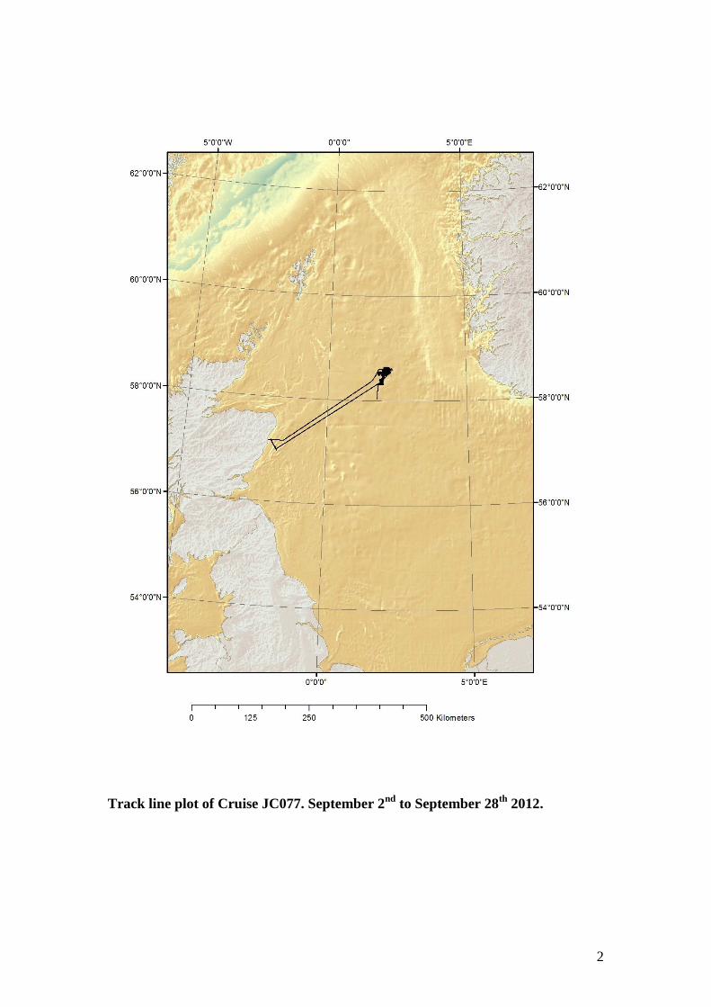
Track line plot of Cruise JC077. September 2

nd to September 28

th 2012.

3

Scientific Party D. P. Connelly NOCS Chief Scientist

B. Alker NOCS Geochemist

J. M. Bull UoS Marine Geophysicist

M. Cevatoglu UoS Marine Geophysicist

M. Esposito UoS Geochemist

M. Hopwood UoS Geochemist

V. Huhnerbach NOCS Marine Geophysicist

T. Le Bas NOCS Marine Geophysicist

A. Lichtschlag NOCS Geochemist

R. Lickorish UoS MSc. Student

E. McDonald UoS MSc. Student

C. Millar UoS MSc Student

J. Pheasant BGS Marine Engineer

C. Richardson BGS Apprentice Engineer

K. Shitashima Uni. Kyushu Sensor Scientist

D. Wallis BGS Marine Engineer

Technical Team

J. Evans NOCS Technical Liaison Officer

D. Childs NOCS CTD Specialist

G. Knight NOCS IT Specialist

S. D. McPhail NOCS Autosub Specialist

D. Paxton NOCS Autosub Engineer

R. Roberts NOCS Marine Engineer

T. Roberts NOCS Marine engineer

Ships Company

J. Leask Master S. Day POD

J. Gwinnell Chief Officer G. Crabb Able Seaman

V. Laidlow 2nd

Officer J. Dale SG1A

P. Munro 3rd

Officer P.Alford SG1A

G. Parkinson Chief Engineer A. Osborne SG1A

C. Uttley 2nd

Engineer I Cantlie SG1A

G. O’Sullivan 3rd

Engineer B. Conteh ERPO

D. Clark ETO D. Caines Head chef

M. Rogers J/ETO M. Ashfield Chef

P. Lucas PCO G. M. Mingay Steward

S. Smith CPOS C. McLaughlin Asst. Steward

P. Allison CPOD

Acknowledgements

The research leading to these results has received funding from the European

Community’s Seventh Framework Programme (FP7/2007-2013) under grant

agreement no 265847 (ECO2). JC077 was funded by the Natural Environment

Research Council.

4

CONTENTS

Section 1. Daily Operation 5

Section 2. Sites of operation 8

Section 3. Autosub6000 25

Section 4. Multibeam 37

Section 5. Hybis 39

Section 6. Biogeochemistry 45

Section 7. Vibrocore Operations 53

Section 8. In situ pH and Eh detection 55

Section 9. NMFSS operations 58

Section 10. Summary and Conclusions 60

Appendix 1 Autosub 6000 Edgetech data processing 61

Appendix 2. Summary of Hybis Dives 64

5

Section 1. Daily Operations

2/9/12

Departed Southampton

3/9/12

Turned on Multi-beam system logging

5/9/12

Arrived on station “Southern Chimneys” site. Did a multibeam/EK60 survey. Did

Autosub deployment. Steamed to “Middle Area”. Did a trial CTD deployment. Did

multibeam survey of Middle Area. Left to pick up AUV.

6/9/12

Continued MB survey of Southern chimney while waited for AUV recovery.

Recovered AUV. Continued multibeam. MB survey over the Northern Fracture.

7/9/12

Did survey over Northern Fracture. Deployed AUV over Middle Area. Started MB

survey over site 3. Moved to Northern Fracture. Did CTD (JC077-CTD002) in

Northern fracture area over bacterial mats identified by Geomar this summer. Did two

vibrocores and got good recovery. Recovered AUV from Middle Area. Did

multibeam to fill gaps over Northern Fracture.

8/9/12

Finished multibeam then did 2 CTD’s and three vibrocores, in the Northern Fracture

area. Deployed Autosub early evening for a survey over the Northern Fracture.

Started a multibeam.

9/9/12

R/V Merion kindly deployed the seafloor lander at 0715 GMT at 58°35.76 N, 02°5.34

E. We recovered AUV, then three CTD’s along the Northern fracture and 3

vibrocores.

10/9/12

Started day with Multibeam survey. Recovered AUV. Two CTD’s and a vibrocore

done over the Northern Fracture area. Multibeam mini-survey followed by AUV

deployment over the Middle Area. Continued multibeam.

11/9/12

Recovered AUV and did two CTD’s. Started multibeam but weather picked up.

Suspended science and steamed towards Aberdeen to pick up Veit Huhnerbach.

12/9/12

Hove too off Aberdeen.

13/9/12

Off Aberdeen storm out at sea.

6

14/9/12

Left Aberdeen in morning to return to study area. Seas rough and we were delayed in

arriving. Multibeam survey over the modelled plume spreading area.

15/9/12

Did a multibeam survey over the spreading plume area. Did a series of 8 CTD casts

across the south, centre and northern part of the spreading plume area. Did two

vibrocores at the Northern Fracture area. Deployed Hybis over the site the Merien

deployed the NOCS lander. Deployed AUV over western Northern Fracture.

16/9/12

Multibeam over Northern Fracture. CTD over wellhead 16/4-2. Recovered AUV.

Vibrocored at the wellhead area. Deployed Hybis on the wellhead.

17/9/12

Started with multibeam and did CTD over the bubble plume area located by Hybis.

Megacores from same site. Vibrocore sample collected over plume spreading area,

deployed AUV same area. Hybis deployment over Middle Area. Multibeam over

plume spreading area.

18/9/12

Finished multibeam survey and then a CTD on the Middle Area. Did megacore and

two vibrocores in the same area. AUV deployment cancelled due to weather.

Multibeam over the plume spreading centre.

19/9/12

Finished multibeam. Did a series of CTD’s over the anomaly areas on the Middle

Area. Weather closed in and had to stop. Tried to launch AUV, but weather too poor.

Did Hybis when weather started to get better in early evening. Multibeam over the

spreading area.

20/9/12

Finished multibeam and did AUV deployment over the Middle Area.

21/9/12

Started with multibeam. Many CTD casts over Middle Area. Vibrocore and megacore

samples collected. Deployed AUV. Multibeam survey through the night.

22/9/12

Finished multibeam survey and recovered AUV. Did CTD survey over Middle Area.

Vibrocore and megacore samples collected at Middle and Northern Fractures.

Deployed AUV. Did megacore sampling over Northern fracture.

23/9/12

Did CTD’s to get a regional view and fill gaps in our study areas. Collected the AUV

and did vibrocores over the Northern Fracture. Did more CTD’s then had to leave

study area because of a very big storm coming.

25/9/12

7

Weather still poor. Did one background CTD.

26/9/12

Did a multibeam survey off Flamborough Head. Did additional background CTD in

shallower water.

End of Science. Returning to Southampton.

Station numbers used during JC077 1. Southern Chimneys

2. Middle Area

3. Bubble site well number 15/9-11

4. Well head 15/9- 16

5. Northern Fracture

6. Area between Northern fracture and Middle Area

7. Fill between Northern fracture and Middle Area.

8. Fill in between MC and BC

8

Section 2. Sites of Investigation Melis Cevatoglu and Jonathan Bull

Several sites chosen for fluid flow investigation during JC077 cruise were the

target of Autosub 6000 science missions (see the table summarizing key information

for each mission).

Figure 2.1. Autosub 6000

1- Southern Chimneys

The 3D seismic data collected by Statoil (1998) reveals the presence of seismic

chimneys in the sediments, 6 km south of the Sleipner platform (Jens Karstens,

personal communication, 2012). These vertical fluid pathways cause strong

amplitudes anomalies on the seismic data. Therefore, this site was the target of

Autosub M59.

Figure 2.2. Seismic chimneys on the south of the Sleipner platform (Jens

Karstens, 2012)

9

2. Middle Area

A similarity analysis of Statoil 3D seismic data (Jens Karstens, 2012) reveals

relatively shallow possible fractures or paleochannels in the sediments, 18km north of

the Sleipner platform. This observation led to several Autosub dives to the area (M60,

M63, M67).

Figure 2.3. Possible fractures on the 18km north of the Sleipner platform with

the black box indicating Middle Area (modified after Jens Karstens, personal

communication, 2012)

3. Northern Fracture

Prior work completed by the University of Bergen in 2011 and 2012 revealed

the presence of a 3km long fracture system c.25 km north of the Sleipner

platform. During JC077 cruise, this fracture was intensively investigated in terms

of its extent and activity (M61, 62, 64).

Figure 2.4. SAS image of the Northern Fracture, 2012 (University of Bergen)

10

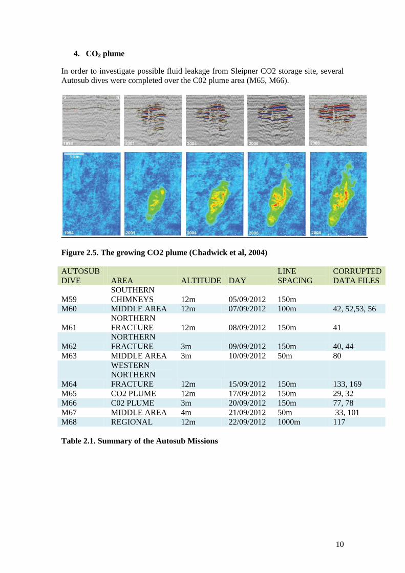
4. CO2 plume

In order to investigate possible fluid leakage from Sleipner CO2 storage site, several

Autosub dives were completed over the C02 plume area (M65, M66).

Figure 2.5. The growing CO2 plume (Chadwick et al, 2004)

AUTOSUB

DIVE AREA ALTITUDE DAY

LINE

SPACING

CORRUPTED

DATA FILES

M59

SOUTHERN

CHIMNEYS 12m 05/09/2012 150m

M60 MIDDLE AREA 12m 07/09/2012 100m 42, 52,53, 56

M61

NORTHERN

FRACTURE 12m 08/09/2012 150m 41

M62

NORTHERN

FRACTURE 3m 09/09/2012 150m 40, 44

M63 MIDDLE AREA 3m 10/09/2012 50m 80

M64

WESTERN

NORTHERN

FRACTURE 12m 15/09/2012 150m 133, 169

M65 CO2 PLUME 12m 17/09/2012 150m 29, 32

M66 C02 PLUME 3m 20/09/2012 150m 77, 78

M67 MIDDLE AREA 4m 21/09/2012 50m 33, 101

M68 REGIONAL 12m 22/09/2012 1000m 117

Table 2.1. Summary of the Autosub Missions

11

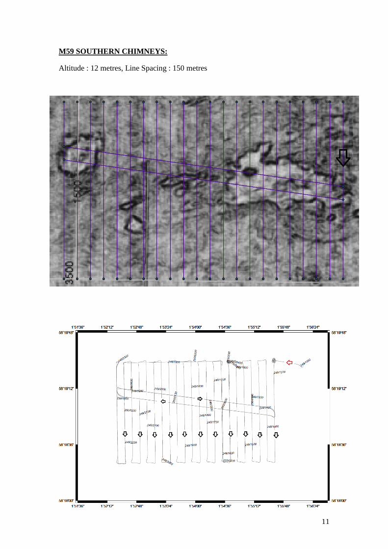
M59 SOUTHERN CHIMNEYS:

Altitude : 12 metres, Line Spacing : 150 metres

12

M60 MIDDLE AREA


13

M61 NORTHERN FRACTURE


14

M62 NORTHERN FRACTURE


15

M63 MIDDLE AREA


16

M64 WESTERN NORTHERN FRACTURE


17

M65 CO2 PLUME


18

M66 CO2 PLUME


19

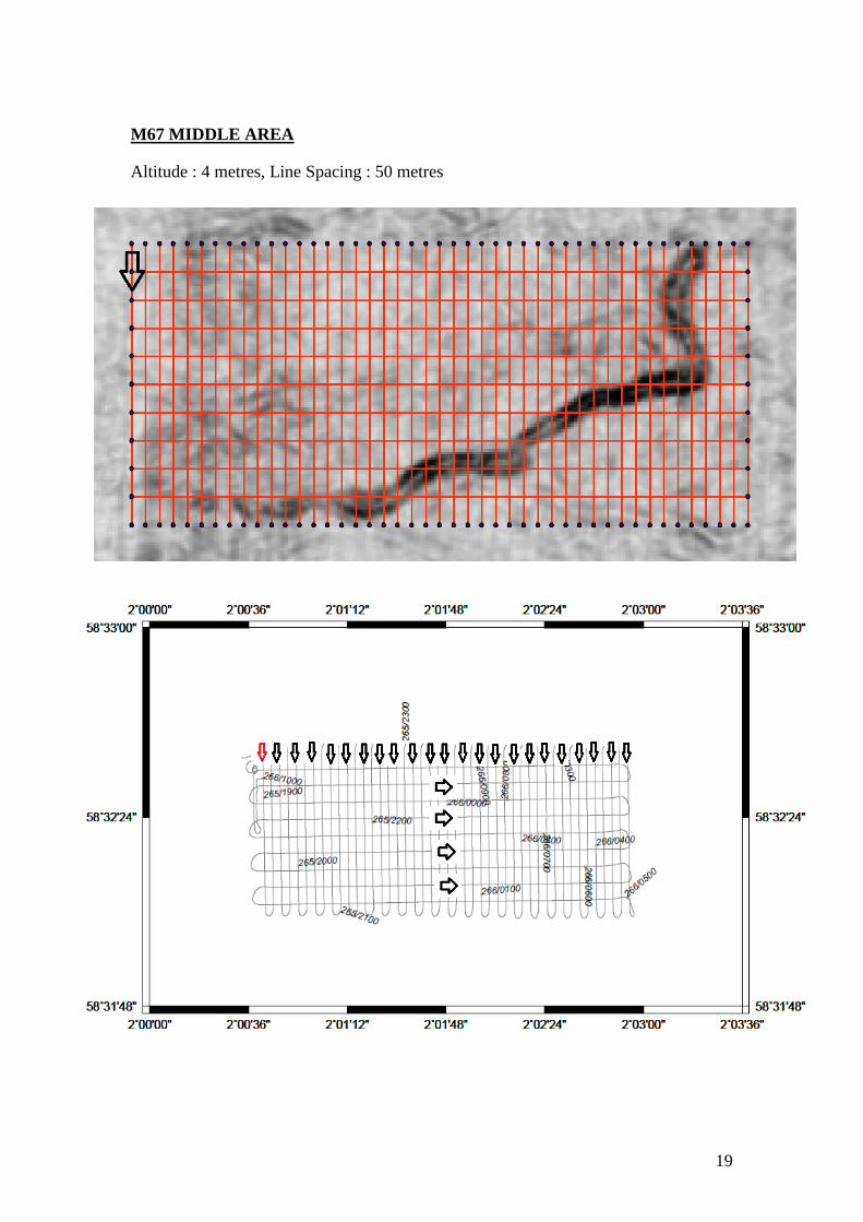
M67 MIDDLE AREA


20

M68 BACKGROUND


21

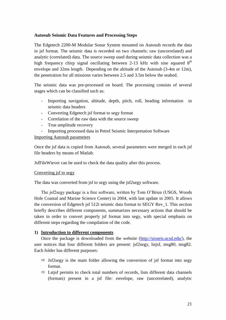
Autosub Seismic Data Features and Processing Steps

The Edgetech 2200-M Modular Sonar System mounted on Autosub records the data

in jsf format. The seismic data is recorded on two channels: raw (uncorrelated) and

analytic (correlated) data. The source sweep used during seismic data collection was a

high frequency chirp signal oscillating between 2-13 kHz with sine squared 8th

envelope and 32ms length. Depending on the altitude of the Autosub (3-4m or 12m),

the penetration for all missions varies between 2.5 and 3.5m below the seabed.

The seismic data was pre-processed on board. The processing consists of several

stages which can be classified such as:

- Importing navigation, altitude, depth, pitch, roll, heading information in

seismic data headers

- Converting Edgetech jsf format to segy format

- Correlation of the raw data with the source sweep

- True amplitude recovery

- Importing processed data in Petrel Seismic Interpretation Software

Importing Autosub parameters

Once the jsf data is copied from Autosub, several parameters were merged in each jsf

file headers by means of Matlab.

JsfFileWiever can be used to check the data quality after this process.

Converting jsf to segy

The data was converted from jsf to segy using the jsf2segy software.

The jsf2segy package is a free software, written by Tom O’Brien (USGS, Woods

Hole Coastal and Marine Science Center) in 2004, with last update in 2005. It allows

the conversion of Edgetech jsf 512i seismic data format to SEGY Rev_1. This section

briefly describes different components, summarizes necessary actions that should be

taken in order to convert properly jsf format into segy, with special emphasis on

different steps regarding the compilation of the code.

1) Introduction to different components

Once the package is downloaded from the website (http://sioseis.ucsd.edu/), the

user notices that four different folders are present: jsf2segy, lstjsf, msg80, msg82.

Each folder has different purposes:

Jsf2segy is the main folder allowing the conversion of jsf format into segy

format.

Lstjsf permits to check total numbers of records, lists different data channels

(formats) present in a jsf file: envelope, raw (uncorrelated), analytic

http://sioseis.ucsd.edu/

22

(correlated) or real for sub-bottom; port and starboard for sidescan) and

provides a few parameters of the jsf file header.

Msg80 and Msg82list some elements of Edgetech message 80/82 jsf files.

They allow the visualization of the total number of records on the jsf input

file, as well as list Side Scan Sonar and Sub-bottom message headers in a

more complete way.

2) Initial commentary

If the user has some prior knowledge about the content of the data collected

and/or has got JsfFileViewer Application (developed by Edgetech itself) to

investigate the input file, the usage of lstjsf, msg80 and msg82 can be skipped.

Otherwise, in order to be able to check if the data is converted properly from jsf to

segy, the input jsf file should be analysed using these three tools.

3) Compilation of the code

Although the code is ready, it should be compiled under a Unix-like environment.

To accomplish the compilation, the user needs to have a look to “Makefile”, present

in each folder: it describes how to compile the related code:

Jsf2segy: gcc jsf2segy.c ascebc.c utils.c –g –m32 –lm –o jsf2segy (compilation of

jsf2segy.c creates jsf2segy command)

Lstjsf: gcc lstjsf.c utils.c –g –m32 –lm –o lstjsf (compilation of lstjsf.c creates lstjsf

command)

Msg80: gcc msg80.c utils.c –g –m32 –lm –o msg80 (compilation of msg80.c creates

msg80 command)

Msg82: gcc msg82.c utils.c –g –m32 –lm –o msg82 (compilation of msg82.c creates

msg82 command)

4) Work with the code

Once the code is compiled, it is sufficient to type commands recently created on

the terminal. This shows how to use the command and its applications.

jsf2segy

[email protected]>jsf2segy

jsf2segy ... extracts sub-bottom data from Edgetech JSF formatted files

Usage: jsf2segy - options first then full path to input file name

Options -e Get Envelope sub-bottom data

-a Get Analytic (correlated) sub-bottom data and make Envelope

-r Get Real sub-bottom data

23

-u Get Raw (uncorrelated) sub-bottom data

-o Path and name of output file

Example: jsf2segy –a Data10.jsf –o Data10.sgy convert analytic (correlated)

Data10.jsf to analytic Data10.sgy

jsf2segy –u Data10.jsf –o Data10.sgy convert raw (uncorrelated)

Data10.jsf to raw Data10.sgy

lstjsf

[email protected]>lstjsf

lstjsf ... Lists Edgetech JSF formatted files

Usage: lstjsf - options full path to input file name

Options -c Get count of Sub-bottom and Sidescan records

-s List Sidescan Sonar message header

-b List Sub-bottom message header

Example: lstjsf –c Data10.jsf Count how many records are in the Data10.jsf file

msg80

[email protected]>msg80

msg80 ... Lists Edgetech JSF formatted files

Usage: msg80 - options full path to input file name




Example: msg80 –s Data10.jsf List Side Scan Message Header of Data10.jsf file

msg82

[email protected]>msg82

msg82 ... Lists Edgetech JSF formatted files

Usage: msg82 - options full path to input file name



24


Example: msg82 –b Data10.jsf List Message Header of the Data10.jsf file

5) Several notes for the user

The original code has been modified to allow the extraction of the raw data

collected by Edgetech 2200-M system. Thus, the actual code can deal both with

uncorrelated (raw) and correlated (analytic) data formats and the segy data can be

easily imported into any seismic processing software.

Correlation of the raw data with the source sweep

After the data format conversion, the source sweep is correlated with the raw data in

promax.

True Amplitude Recovery

A basic processing is applied to the seismic data in order to recover amplitudes, lost

by spherical attenuation.

Importing data in petrel

Some of the lines are imported in petrel seismic interpretation software to check their

quality.

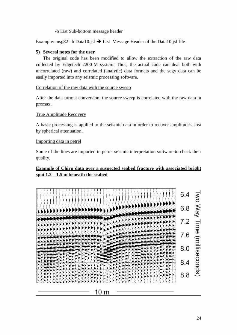
Example of Chirp data over a suspected seabed fracture with associated bright

spot 1.2 – 1.5 m beneath the seabed

25

Section 3. Autosub6000.

Steve McPhail

Mission Summary

There were a total of 10 successful science missions. 708 km of lines track was

surveyed over a period of 141 hours with a combination of: HFSSS (410 kHz)

sidescan sonar, Chirp Profiler, a 5 M Pixel digital colour camera stills, pH, Eh, CTD

with DO , and light back scatter sensors.

The availability and operating reliability were 100%, and the data return rate from the

sensors was also 100% except for a small percentage of the Edgetech files which were

unreadable due to some corruption in the data written to disk. These are probably

recoverable (Edgetech will be contacted).

Table 3.1 is a general summary of the Autosub6000 missions on JC060.

# Start and end

date & time

[GMT]

Mis

sion

Dur

atio

n

Hrs

Location Start Position Ma

x

Dep

th

(m)

Altit

ude(s

) [m]

Dista

nce

travel

led

[km]

59 05-Sep-2012

13:02:08

06-Sep-2012

03:59:30

15.0 Seismic

Chimneys

N:58:19.505,E:1:5

5.600

81 12

and

3.2

72

60 07-Sep-2012

06:58:54

07-Sep-2012

20:54:16

13.9 Middle

Area

N:58:32.892,E:2:0.

687

87 12

and

3.2

70

61 08-Sep-2012

18:44:04

09-Sep-2012

08:53:24

14.2 Northern

Fracture

N:58:36.315,E:2:5.

544

80 12

and

3.2

70

62 09-Sep-2012

21:43:28

10-Sep-2012

11:49:12

14.1 Northern

Fracture

N:58:35.240,E:2:5.

720

88 3.2 71

63 10-Sep-2012

20:56:28

11-Sep-2012

06:44:58

9.8 Middle

Area

N:58:32.622,E:2:0.

694

83 3.2 49

64 15-Sep-2012

22:38:25

16-Sep-2012

14:49:09

15.0 Northern

Fracture

N:58:36.293,E:2:2.

137

75 12.0 75

65 17-09-2012

18:08:04

14.6 Sleipner

CO2

N:58:24.326,E:1:5

7.653

70 12.0 73

26

18-Sep-2012

07:36:14

plume

66 20-Sep-2012

08:34:34

20-Sep-2012

21:48:22

14.6 Sleipner

CO2

plume

N:58:24.326,E:1:5

7.653

79 3.0 73

67 21-Sep-2012

18:58:46

22-Sep-2012

09:24:40

14.4 Middle

Area

N:58:32.622,E:2:0.

694

80 4.0 73

68 22/09/2012

18:53:10

23-Sep-2012

11:06:34

16.2 Connecti

ng all

three

areas

N:58:34.924,E:1:5

9.388

72 12 m 83

Navigation Performance

The JC077 missions were interesting for the evaluation of the navigation performance

of Autosub6000, as the shallow depth meant that continuous bottom track navigation

was possible between the start and the end GPS fixes. In addition, with pipelines

intersecting many of the tracks, it was possible to evaluate the navigation drift on a

track by track basis.

There were two main issues affecting the accuracy of the navigation, and of merging

of the navigation and Edgetech data.

1) Increased variance of velocity measurement at 3 m altitude, compared to

missions at 12 m altitude.

2) Lack of Synchronisation between the Edgetech logger and the AUV

navigation logger.

Figure 3.1 illustrates the first issue. The standard deviation in north velocities for

Mission 64 (blue) at 0.016 m/s are significantly less than those for mission 66 (red) at

0.099 m/s.

27

Figure 3.1. Increased velocity measured variance at low altitude. Red trace is for the 3

m altitude mission, the blue for the 12 m altitude mission.

The effect of this variance is enough to produce noticeable offsets on a line by line

basis, and explains the larger final GPS position fix jump for the missions run at 3 m

altitude compared to the missions run at 12 m altitude. The manufacturers of the

ADCP used for navigation (Teledyne RDI) discuss use of a different operating mode

for low altitude operation, giving significantly reduced variance. However during the

cruise it was considered too risky to change the operating mode of the ADCP, and

hence this was not tried.

Table 3.2 is a summary of the average navigation drift as measured by comparing the

dead reckoned position with the GPS fix at the end of the mission.

The lack of synchronisation between the Edgetech logger and the AUV logger meant

that to match the Edgetech sonar data with the navigation, we first measured, then

corrected for, the relative clock drifts in the post processing. However, since the

relative drift rates were both quite large (of order 50 to 100 ppm) and variable, then

the resulting uncertainty in position due to this cause could be of order 2 m.

.

0.8 1 1.2 1.4 1.6 1.8 2 2.2 2.4

x 104

-1.5

-1

-0.5

0

0.5

1

1.5

Mission 64 and Mission 66 North Velocities

Data Count (every 2 seconds)

Nort

h V

elo

cit

y (

m/s

)

28

# Flying

Altitude

N

drift

(m)

E drift

(m)

Drift Rate

(km/hour)

59 12 4.0 23.1 1.4

60 12 -

16.8

39.0 2.9

61 12 -

11.4

-29.3 2.3

62 3.2 -

20.7

8.9 2.6

63 3.2 NA1

NA1

NA1

64 12 15.9 21.2 2.1

65 12 -

27.5

-2.1 2.0

66 3 4.1 -79.6 5.9

67 3 48.7 49.0 4.7

68 12 -

13.2

11.6 1.0

Table 3.2 Summary of Navigation Drift for the 10 missions. For Mission 63 [1], a

navigation offset command was sent to the AUV when it was subsurface in order to

safely avoid fishing boats. The effect of the offset was that the navigation system

rejected the GPS fixes when the AUV surfaced, as it calculated them to be outside of

sensible range. Note the worse drifts at the lower altitudes.

Sonar devices installed on Autosub6000

The system consists of a dual 120 kHz, 410 kHz sidescan system, with a 2 to 15 kHz

sub bottom profiler. The one way beam width is reported to be 0.3 degree for the 410

kHz, and 0.8 degree for the 120 kHz. On JC077, only the HF (410 kHz SSS) and

SBP was used.

Autosub Sensor Configuration

The sensor suite fitted to Autosub6000 are listed in Table 1. Photographs 1 to 6 show

the installation of the CTs, Oxygen, EH, camera and flash, multi beam, side scan and

sub bottom profiler. Each CT assembly was mounted on the inside of the nose panel

with a 40mm (i.e. short) length of tube plumbing the water outside the vehicle to the

temperature sensor (photo 1).

The Edgetech sub bottom profiler (SBP) was mounted in the tail section with the

receivers were mounted outside the vehicle on the centre section (Photo 8, 9).

Table 3.3. Autosub sensor suite for JC0060

Description Part No. Source Serial No.

CTD Port Temp 90565 Sea Bird 03P5009

CTD Port Cond’ 90468 Sea Bird 043499

CTD Stbd Temp 90465 Sea Bird 03P5071

CTD Stbd Cond 90468 Sea Bird 043566

29

Oxygen sensor 90599.2 Sea Bird 431582

CTD Pump Port 90544 Sea Bird 055125

CTD Pump Port 90544 Sea Bird 055238

CTD Logger 90538.042 Sea Bird 09P52764-

0930

EH Sensor Ko-ichi

Nakamura

PH Sensor Kiminori

Shitashima

Light Scattering

Sensor (LSS)

Sea Point

300 kHz ADCP RDI-Teledyne

Depth sensor NOC dwg No

A5952

Digiquartz Inc.

Camera 5 M pixel colour (see later

section for details).

Side scan,

Sub bottom

profiler

Edgetech 2200 system. Only the

410 kHz (HFSSS) and Chirp

profiler were used on this cruise.

Photo 1. Port CT (mounted below the panel split line) and Oxygen sensor uppermost

30

Photo 2 EH sensor on starboard side protruding through panel. PH sensors were

also mounted in this position.

Photo 3. Edgetech electronics mounted in the tail

31

Photo 4. Edgetech Side Scan inset into the centre buoyancy blocks just below the

winglets

Photo 5. Looking up at the tail section, ‘bumble bee’ tape covers the aperture cut for

the SBP transmitter.

Photo 6. Sub bottom profiler receivers (bottom of photo) mounted outside vehicle

32

Launch and recovery

The new Lawson Engineering Ltd gantry was mounted on the port side ‘ROV

position’. The equipment performed well and most launch and recoveries were

without drama. As with previous side launch positions, the AUV was set running for

30 seconds away from the ship as soon it hit the water; this was fond in practice to be

essential due to the suction effect near the ship. The biggest problem was the lack of

visibility for the bridge from this position. Initially the lines were grappled just aft of

the gantry position, but visibility being particularly bad for this position, grappling

was moved to the port quarter, with more success. The grapple gun achieved only 3

hits, due partly to good throwing arms of the deck seamen. The AUV washing line

was extended into the tail and nose sections, much easing grappling.

.

Photo7. The Autosub6000 MKII L&R system installed on the aft deck of the RRS

James Cook. The red tape (rather comically) showing the position of some top panel

damage due to ship collision on the last recovery

33

Autosub 6000 Data Files and Formats

Autosub6000 Files Handed over for JC077.

Cruise Summary Files and Sensor Calibration Data.

Filename Description Cruise Report Autosub JC077.docx Cruise Report - THIS JC077 Data Handover Files and

Formats.docx

JC077 Autosub Missions Summary.xlsx Summary information for all the missions, including

start and end times, start positions, JC077 Cameras Setup and Files.docx Detailed information on the Camera Setup and file

formats. JC077.con The calibration file for the CTD.

Files for Each Mission M059 through to M068

Separate large files for the Edgetech and the Camera systems.

Folder/ Filenames Description /M0XXEdgetechData/DATA0000001X.jsf Edgetech .jsf files. For Mission 59 these were 10

minute files. For Mission 60, new files were started

at the beginnings of lines, with a ten minute timeout.

For all subsequent files the time limit was 30

minutes, and new files were produced for each line.

For Mission 68, with 20 km long lines there are

several files per line. /MXX_05092012_123052_10441297/ MXX_10441297_xxxxxxxxxxxxxx.raw

Raw format Camera Image data. One every 0.8

seconds of all the missions.

Navigation and Sensor Data Files. In JC077final26thSeptember.zip zip archive.

Example for Mission 060:

M060_Mission Info.txt Some basic Mission Information. Start and end times, survey duration

and most common values of water depth, AUV depth and AUV

altitude. M060_PHSensorData.csv All sensor (except Edgetech or Camera) on a common time base with

the AUV post processed navigation data. Comma separated values,

with time in excel format. Format description. M060_Sensors.mat Matlab version of the above file. Format description. _10HzM060.mat The 10 Hz up-sampled version of the post processed AUV navigation

data, with the timebase adjusted to the offset and drift rate of the

Edgetech raw clock (the .jsf files). Format description. M060_EdgeTechNav.txt Text file with the post processed AUV navigation (as above), time

corrected to align with the Edgetech data. Format description. M060cam.txt_imageData.

csv File with the post processed navigation data for each of the camera

frames taken. Format description. M060ETtimeOffset.m The time offset and drift rates of the Edgetech logger compared to the

AUV navigation logger. Note that this is for information only. The

corrections have been already applied to the applicable files.

34

M060NavPerformance.txt A measure of how far the dead reckoned navigation had drifted during

the submerged portion of the mission. This is for information only, the

applicable correction has already been applied to the post processed

navigation data. FiguresM060 (Folder) A series of figures of the 2 D scatter (longitude, latitude as X, Y, and

the signal colour coded). pdfs and Matlab versions. The Matlab

versions are more generally useful as the figures can be zoomed, and

more usefully the range of the colour scale changed. The figures which

are “high passed” are high passed filtered (achieved by subtracting

low pass filtered version of data) , in order to remove the low

instrument drift , and emphasise the short term changes in the data.

Include, also, a time series of all the sensor data. The high passed filter

time constant is 30 seconds.

Time Offset Issues between the Edgetech and the Autosub logger clocks

The reference time for all Autosub6000 sensor data is the clock on the Autosub6000

logger. This maybe a few seconds difference from UTC, but this is no practical

importance.

Unfortunately, it was not possible to synchronise the clocks on the Edgetech system

with the times on the logger, hence there is a time offset and drift between the two.

As a work around for this problems, prior to each mission dive, and post the surfacing

of the AUV, a program running on a lab computer measured the relative differences

between the Autosub logger and the Edgetech clocks, from which the offset (at the

dive time), and the rate of drift was calculated.

This time offset and rate for each dive is stored in a file MXXXtimeOffset.m

For the data which is used for matching of the Edgetech data with the logger

navigation data, this offset and rate are applied to the logger data. Hence for the files,

e.g. Mission M060 :

M060_EdgeTechNav.txt, and _10HzM060.mat This offset has been already applied.

So it should be remembered that for only these particular files, the clock has been

adjusted to be synchronised with the Edgetech time.

Autosub File Formats

MXXX_PHSensorData.csv:

Format: ASCII Text. Comma Delimited. The Date format is readable directly by

excel as date/time. There is a one row header.

For each value recorded for the Kiminori Shitashima pH sensor, there is a set of

navigation data.

All the navigation data is based on the post processed navigation (includes the

correction applied after the GPS fix at the end of the mission).

35

Name Unit Description MissionName # e.g. M060 Mission Date Excel Time Latitude Degrees e.g. 58.123456 Positive is North. Ref geoid is WG84 Longitude Degrees e.g. 1.123456 Positive is East. Depth m AUV depth in m. Deeper is more positive. Altitude m AUV Altitude off seabed (measured by ADCP) PitchDeg Degrees AUV Pitch (nose up is positive) RollDeg Degrees AUV Roll (nose down is positive) HeadingDeg Degrees AUV Heading (normal navigation sense – east is 90

degrees) Ground Speed m s

-1 Speed relative to see bed. Eh see CTD cal CTDPres dBar S1 psu S2 psu T1 Celsius T2 Celsius DO See CTD cal LSS See CTD cal d1 unknown –

refer to

Kiminora

Shitashima

t1 “ d2 “ t2 “ d3 “

MXXX_Sensors.mat

The format is a Matlab variable ‘PH’ with the structure elements identical in meaning

to those (above) for the ASCII ‘MXXX_PHSensorData.csv’, with one exception: The

time variable ‘PH.eTime’ is the number of seconds since 1/1/1970.

_10HzMXXX.mat

This file was produced to enable AUV navigation data to be inserted into the

Edgetech jsf header files.

This Matlab file with up-sampled (from 0.5 Hz to 10 Hz) post processed (for end

GPS position) navigation data. The navigation is smoothed with a time constant of 30

seconds with a filter designed to give minimal time lag. The timebase has been

adjusted to be as close as possible matching the Edgetech Clock, using the measured

offset and drift rate of the Edgetech clock relative to the Autosub Logger clock. The

data field are:

usAltitude m AUV Altitude off seabed (measured by ADCP) usDepth m AUV depth in m. Deeper is more positive. usHeading Degrees AUV Heading (normal navigation sense – east is

90 degrees) usEast Degrees e.g. 1.123456 Positive is East.

36

usNorth Degrees e.g. 58.123456 Positive is North. Ref geoid is

WGS 84 usPitch Degrees AUV Pitch (nose up is positive) usRoll Degrees AUV Roll (nose down is positive) usSpeed m s

-1 Speed relative to see bed. usTime seconds Number of seconds since 1/1/1970. The time

increment is 0.1 seconds. The time is offset and

drift corrected to match that of the Edgetech

time stamp.

MXXX_EdgeTechNav.txt

The file is a fixed field format for importing into the Edgetech HFSSS processing

software. The number of white spaces is important for correct parsing.

e.g.:

Mission Date Time NorthDeg EastDeg HeadingDeg RollDeg PitchDeg Depth

Altitude Speed

M066 120920 082757 58.405140 1.961891 194.758 -16.366 0.451 10.057

74.468 1.044

The fields are self explanatory and defined the same as for the _10HzMXXX.mat.

MXXXcam.txt_imageData.csv

This file gives (post processed) navigation data for each frame taken by the Autosub

downward looking camera. For more information see: ‘JC077 Cameras Setup and

Files.docx’

FIELD DESCRIPTION Time Time of frame in excel format (days since 1900). Altitude_m Altitude of AUV in m. Is set to ‘NaN’ if no data (> 200 m altitude). The AUVdepth_m AUV depth in m. Interpolated for each frame. WaterDepth_m The water depth is AUV depth plus AUV altitude. (NaN if no valid altitudes). Is

interpolated for each frame. Latitude_deg The decimal latitude in degrees. This is post processed navigation, low pass filtered to

reduce jitter, and interpolated for each frame. Longitude_deg The decimal Longitude in degrees. This is post processed navigation, low pass filtered (with

zero delay) to reduced jitter, and interpolated for each frame. Pitch_deg AUV pitch (positive is nose up) in degrees. Interpolated for each frame. Roll_deg Roll (positive is starboard down). Interpolated for each frame. Heading_deg Heading (positive clockwise from north). Interpolated for each frame. Frame_Filename The Filename is e.g. M55_11370385_12987210455670.raw. Mission Number/Serial

Number of Camera/timestamp milliseconds since the start of 1700.The raw is format at 8

bits per pixel.

37

Section 4. Multibeam Tim Le Bas

Multibeam bathymetry (EM710)

The shipboard multibeam shallow water system (EM710) was used regularly during

the cruise. It collected over 600 files each of about 750Mb for each 30 minutes of

data. This was unusually large due to the inclusion of the water column data within

the files. For future cruises collecting this water column data, it is recommended that

this is to be held on separate files as it slowed the bathymetry processing

considerably. Bathymetry data were processed in CARIS HIPS v7.1.1. The data was

corrected with a sound velocity provided by a CTD dip. No tidal correction was done

but this did not seem to affect the data.

A calibration survey for transducer orientation was conducted just offshore Aberdeen

and a value of -4.0 degrees was found for pitch and 0.34 degrees for roll.

The bathymetry values varied between 80m and 111m though a lot of noise was also

present and required considerable manual editing to remove outliers. Lines travelling

east to west were particularly noisy in comparison to the reverse direction. Lines

were spaced at 250m. Some small holes in the survey are due to bad weather or

suspension of survey lines to go to sampling stations. Some lines were repeated to

improve on the previous poor data. Final data coverage was 246 sq km at a resolution

of 5m.

Multibeam backscatter (EM710)

As with the bathymetry system the backscatter data did suffer from poor data quality.

Data were converted and transferred to the PRISM (v5) system for processing. Ship

track lines were extracted from the stored data and 15 map areas chosen, as the

coverage was too large for a single map. Due to the poor signal-to-noise ratio the

backscatter mosaic was done at 2.5m whereas it would be hoped to be done at 1m.

Survey speed was about 6 knots and pulse repetition was about 0.5 seconds and thus

ping spacing was about 1.5m. Repeat surveyed lines were handled separately and

mosaiced on top of the original data. The PRISM Processing configuration was:

mrgnav -i %1 -o %0 -n navfile.nav -l 0,0

sshead -i %1 -o %0 -a 2.0

filter -i %1 -o %0 -b 1,21 -z -v 130,255

filter -i %1 -o %0 -b 1,301 -h -v 130,255

filter -i %2 -o %0 -b 31,301 -L -v 130,255

wtcombo -i %2 , %1 -o %0 -c 1,1 -a -128

restorehdr -i %1 -h %5

resol -i %2 -o %0 -a -r res

shade -i %1 -o %0 -n 128 -t 1,254

38

Autosub 6000 Edgetech Sidescan

Following each Autosub deployment the jsf data was downloaded from the vehicle

and transferred to the PC replay system (Discover 4200 MP 2.03). Data were

replayed thus allowing it to be viewed and converted into xtf format. This is a slow

and laborious process typically taking over an hour per mission. Some difficulties

were encountered when replaying the data and some coverage was lost. A table of the

missions and the data files lost is provided. The amplification gains are set by the

user according to the sidescan values. These were kept constant for each deployment

and were generally set according to their programmed mission altitude:

12m altitude 29dB for Gain and 18dB for TVG over 100m

3m altitude 25dB for Gain and 20dB for TVG over 100m

Data were converted and transferred to the PRISM (v5) system for processing.

Navigation for Autosub is provided separately and this was imported from a

spreadsheet. The sidescan mosaic was generally done at 0.5m though some smaller

specific areas were processed at 0.1m. Survey speed was about 2.8 knots and pulse

repetition was about 0.21 seconds and thus ping spacing was about 0.3m. The PRISM

Processing configuration was:

widealt -i %1 -o %0 -p

mrgnav_inertia -i %1 -o %0 -u 0 -r 0.0,0.0 -n navfile.veh_nav

edge16 -i %1 -o %0 -m

tobslr -i %1 -o %0 -r0.0576 , res # HF 110m 6 Hz subsamp 5

shade_tobi -i %1 -o %0 -n 1000

foldtobi -i %1 -o %0 -t 3000

filter -i %1 -o %0 -b 1,351 -h -v 1,5000

filter -i %2 -o %0 -b 21,351 -l -v 1,5000

wtcombo -i %2 , %1 -o %0 -c 1,1

restorehdr_tobi -i %1 -h %5

mrgheading -i %2 -o %0 -f -t -n navfile.nav

It was found that the Autosub navigation for the 12m altitude sidescan imagery

matched the features very well to shipboard multibeam backscatter imagery. Features

that crossed from pass to pass such as pipelines or cables matched well with errors

being less than 2m. However the 3m altitude imagery deployments showed

considerable error in positioning, accumulating error as the mission continued. Some

features were measured to be 75m offset from the 12m altitude data. New navigation

files were provided and these occasionally improved feature matching.

The processed mosaics were then transferred to the GIS along with a navigation

overlay with acquisition times. It was also noted that when Autosub turned from line

to line about 8 seconds of data (40 pings) were lost. As these were at the end of the

lines it was not considered problematic.

Full instructions for processing are included in Appendix 1.

39

Section 5. HyBIS operations during JC77 Veit Huhnerbach

The HyBIS vehicle

HyBIS is a simple, low-cost, multi-purpose, survey and sampling robotic underwater

vehicle (RUV) with a depth capability of 6000m (Fig 5.1). It was designed and built

in the UK by Hydro-Lek Ltd. in collaboration with the National Oceanography

Centre, Southampton (NOC), back in 2008. Since then, the vehicle has had 3

successful trials cruises and completed 9 scientific expeditions, from the Arctic to the

Tropics.

The vehicle has a modular design that make its very versatile, with the top module

being a command and power system that comprises power management, cameras,

lights, hydraulics, thrusters and telemetry. Telemetry is via a single-mode fibre optic

link and provides 3 channels of real-time standard-definition colour video plus vehicle

attitude data. Power is supplied through a single-phase 1500V ac, 8kVA umbilical

and converted to 3-phase 120V on the vehicle by two silicon motor controllers, 240V

ac for the lights, and 24 to 12V dc for onboard instruments.

The easily changeable lower modules available at the moment include a clam-shell

sampling grab, a 5-function manipulator-arm and tool sled, a winch with 600m rope

for instrument recovery and an ocean bottom seismometer deployment module. The

sampling module used during JC77 during the video surveys comprised a 0.5 cubic

metre clam-shell grab with a pay-load capacity of 750kg and closure force of 4

tonnes. 5 sediment samples were taken during the voyage 77 of RRS James Cook.

Unlike a conventional ROV, HyBIS does not have any floatation or buoyancy, it is

rather suspended by its umbilical cable directly from the ship which makes it slightly

susceptible to ship roll and heave motion, especially in the shallow water depths in

this working area. On the positive side, the advantage of direct suspension is that

HyBIS can recover or deploy a payload of up to 750kg.

40

Figure 5.1 Hybis vehicle

Laboratory control unit setup

The top-side control centre (Figure 5.2) was established in the main science lab, on

starboard side, right next to the HV cage and the junction boxes for fibre-optics and

power. The vehicle’s primary control box was supplemented with additional monitors

and a relay of the USBL navigation screen. A dedicated GPS aerial was mounted on

an out-rigger over the starboard side and provided a continuously recorded GPS string

to the Garmin GPS navigation system in the control box. Unfortunately, the GPS

signal was lost on several occasions due to the location of the GPS antenna which was

limited by the length of its cable. Winch controls were established adjacent to the

vehicle pilot’s position, allowing synchronisation between winch operator and pilot.

Video was recorded digitally as DV and AVI formats on 2Tb hard-discs. Two

cameras (forward and downward SD) were recorded continuously in standard

definition. The forward looking camera with vehicle attitude data overlain was also

recorded on DVDs of about one hour length. Full HD video (1080i, PAL, 30fps,

AVCHD format) was not used. Back-ups of all dive data and videos were then made

on regular intervals. All GPS navigation data were recorded on the top-side command

unit and copied to a USB portable drive. Time codes were all set and synchronised to

GMT.

Acoustic navigation was provided using the vessel’s Sonardyne USBL tracking

system with a mini-transponder beacon on the HyBIS vehicle. Tracking was generally

good although transponder battery conditions provide a limited maximum dive time

of about 6-8 hours until recharge becomes necessary. The computing representative

onboard recorded all available USBL navigation data.

41

Figure 5.2. left to right, top to bottom: Lab setup showing video screen and

logging system arrangements for HyBIS and its main control box.

High-voltage power setup

Prior to the HyBIS HV transformer being installed in the main lab, a lockable

enclosure (Fig xxx) needed to be installed in order to comply with UK high-voltage

regulations. HV safe working procedures were put in place, and kindly overseen by

the HV responsible person Ian Pheasant (BGS), which meant that HyBIS was not to

be switched on prior to deployment and recovery. All procedures were communicated

to and agreed with the crew. HV working permits were issued and signed off for each

deployment. In addition, an area of the mid-ship deck, just outside the CTD wet lab

was cordoned off during all HV operation.

Before recovery of the vehicle, tests were made to ensure that no residual current was

left in the deep-tow cable, allowing safe handling onto the deck. In addition, an

earthing rod was attached as additional safety.

42

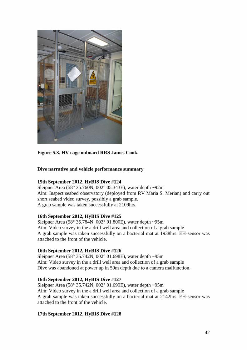
Figure 5.3. HV cage onboard RRS James Cook.

Dive narrative and vehicle performance summary

15th September 2012, HyBIS Dive #124

Sleipner Area (58° 35.760N, 002° 05.343E), water depth ~92m

Aim: Inspect seabed observatory (deployed from RV Maria S. Merian) and carry out

short seabed video survey, possibly a grab sample.

A grab sample was taken successfully at 2109hrs.



Aim: Video survey in the a drill well area and collection of a grab sample

A grab sample was taken successfully on a bacterial mat at 1938hrs. EH-sensor was

attached to the front of the vehicle.




Dive was abandoned at power up in 50m depth due to a camera malfunction.




A grab sample was taken successfully on a bacterial mat at 2142hrs. EH-sensor was



43


Aim: Video survey of the seabed

EH-sensor was attached to the front of the vehicle.











Aim: Video survey of the seabed and collection of a grab sample

A grab sample was taken successfully on a high-backscatter mound feature at 0032hrs

(19th

September). EH-sensor was attached to the front of the vehicle.




EH-sensor was attached to the front of the vehicle. Dive was cut short due to the

USBL battery being discharged. No GPS on the vehicle overlay data at the beginning

of the dive.







Aim: Video survey of the seabed along Northern Fracture and collection of a grab

sample

A grab sample was successfully taken on bacterial mats at 0221hrs. EH-sensor was


With almost 13 hours of seabed video survey time and 5 grab samples, HyBIS was an

integral part of the science program for the second part of the cruise. The video

surveys helped ground-truthing the extensive acoustic surveys of the AUV and ship-

borne equipment, and the grab samples brought sediment and biological samples

onboard.

The integration of the Eh-sensor (Fig 5.4) also allowed continuous measurements

during the HyBIS dives. Its results showed PH-changes over limited small scale

features that indicated possible venting activity.

44

Figure 5.4. EH-sensor (left side) attached to the HyBIS vehicle

HyBIS operations were stopped on the evening of September 21st due to damage of

the fibre-optic cable during the changeover from Megacoring to HyBIS. Re-

termination took until midnight of that day. The, almost daily, changeover of the

cables and consequent terminating and disconnecting of the vehicle was not ideal, but

unavoidable to allow continuous science operation.

Upcoming bad weather conditions led to the cancellation of all further HyBIS

operations planned for the remainder of the cruise.

45

Section 6. Water column and sediment (bio)geochemistry Anna Lichtschlag, Douglas Connelly, Mark Hopwood, Mario Esposito, Belinda

Alker,

Background

The aim of the (bio)geochemical water column and sediment sampling and

analyses during this cruise was to: search for tracers of leakage of formation fluids or

precursors from the spreading sub seafloor CO2 plume at the Sleipner CCS site, to

identify potential mobilization of toxic metals by CO2, and to characterize the

environment in the vicinity of the Sleipner storage site.

The main target areas for sediment sampling were the newly discovered

”Middle Area” Station 2, about 18 km north of Sleipner, the “Northern Fracture” area

about 25 km North of Sleipner (Station 5) and the ”Area above the spreading CO2

plume at Sleipner” (Station 7). In order to monitor the distribution of solutes and

solids at these potential CO2 seepage sites, long sediment cores were retrieved with

the vibrocoring technique (VC, maximal length 3.79 m, Fig. 6.a). As occasionally the

upper sediment layer is lost during vibrocoring, sediment sampling was

complemented by retrieving undisturbed sediment surface samples using a Megacorer

(MC, maximal length 15 cm, Figx.1b). Altogether 12 VC and 5 MC were sampled

for geochemical analyses and for each core a duplicate core was taken to be archived

and used for later mineral analyses Table x.1/Table x.2.

Localisation of possible seepage and determination of background

concentration was performed by CTD measurements and water sampling. Here, in

addition to the above mentioned target sites, the “Southern Chimneys” (Station 1), the

“Bubble Site Well Number 15/9-11” (Station 2), the “Well Head 15/9-16” (Station 4),

and the “Area between Northern Fracture and Middle Area” (Station 6) were sampled.

Sea water samples were collected from a total of 63 CTDs across the 7 areas of

interest. Table X.

46

Figure 6.1 a) Vibrocore sampling b) CTD sampling and c) a megacore sample

Event Area Label Latitude(N) Longitude (E)

Water

depth

(m)

Purpose Length of

Core (m)

71 5 JC077-

VC01 58.5947167 2.08823333 94

Geochem. 2.92

72 5 JC077-

VC02 58.5947167 2.08823333 94

Archive 2.88

72 5 JC077-

VC03 58.5956167 2.08898333 94

Geochem 2.95

92 5 JC077-

VC04 58.5959833 2.08895 94

Geochem. 3.30

93 5 JC077-

VC05 58.5959833 2.08895 93

Archive 2.81

93 5 JC077-

VC06 58 35,762 2 04.965 93

Geophysics 3.49

114 5 JC077-

VC07 58.5960333 2.08021667 94

Archive 3.37

115 5 JC077-

VC08 58.5960333 2.08021667 94

Geochem. 3.50

141 5 JC077-

VC09 58.5957667 2.08021667 93

Archive 3.35

142 5 JC077-

VC10 58.5957667 2.08021667 93

Geochem. 3.79

183 5 JC077-

VC11 58.59325 2.0676 92

Archive 3.15

184 5 JC077-

VC12 58.59325 2.0676 92

Geochem. 2.60

201 5 JC077-

VC13 58.59305 2.06816667 93

Archive 2.38

202 5 JC077-

VC14 58.59305 2.06816667 93

Geochem. 2.46

220 7 JC077-

VC15 58.3745167 1.95128333 83

Geochem. 2.35

248 2 JC077-

VC16 58.5373 2.01418333 89

Geochem. 2.82

249 2 JC077-

VC17 58.5373 2.01418333 89

Archive 1.92

250 7 JC077-

VC18 58.3749167 1.95095 81

Archive 2.70

286 7 JC077-

VC19 58.3837833 1.95385 84

Archive 1.60

287 7 JC077-

VC20 58.3837833 1.95385 84

Geochem. 3.20

316 5 JC077-

VC21 58.5957833 2.02843333 96

Archive 1.86

317 5 JC077-

VC22 58.5957833 2.02843333 96

Archive Not

collected

318 5 JC077- 58.5957833 2.02843333 96 Geochem. 1.94

47

VC23

340 2 JC077-

VC24 58.5389667 2.01421667 89

Geochem. 2.98

341 2 JC077-

VC25 58.5389667 2.01421667 89

Archive 1.54

342 5 JC077-

VC26 58.5958167 2.08271667 93

Geophysics 3.1

377 5 JC077-

VC27 58.5960167 2.08248333 93

Archive 1.63

378 5 JC077-

VC28 58.5960167 2.08248333 93

Geochem. 3.0

Table 6.1 Vibrocore sample information

Event Area Label Latitude(N) Longitude (E) Water depth (m)

217 5 JC077-MC1 58.5908 2.02373 95

247 2 JC077-MC03 58.5373 2.01418 89

288 7 JC077-MC04 58.3837 1.95377 84

296 5 JC077-MC12 58.5959 2.08878 93

297 5 JC077-MC13 58.5929 2.06677 93

319 5 JC077-MC18 58.5958 2.0284 95

356 5 JC077-MC31 58.596 2.08248 92

Table 6.2 Details of Megacores, From each station one core was used for

geochemical measurements and a 2nd

one was archived.

No. Lat °N Long °E Bottles fired Depths (m)

1 58° 31.08 1° 57.19 1-5 77, 5 2 58° 35.683 2° 05.294 1-15 76, 74, 70, 66, 60 3 58° 35.762 2° 04.965 1-15 84, 8, 75, 70, 5 4 58° 35.737 2° 05.339 1-15 80, 78, 74, 67, 8 5 58° 35.745 2° 04.816 1-15 88, 85, 82, 78, 5 6 58° 35.618 2° 04.036 1-15 84, 82, 79, 73, 7 7 58° 35.387 2° 02.925 1-15 88, 86, 84, 79, 7 8 58° 35.624 2° 03.986 1-15 85, 83, 80, 75, 6 9 58° 35.743 2° 04.814 1-15 87, 84, 81, 77, 5 10 58° 35.592 2° 04.128 1-15 87, 84, 81, 77, 5 11 58° 35.606 2° 04.096 1-15 89, 87, 85, 79, 5 12 58° 22.403 01° 56.792 1-15 75, 73, 70, 65, 5 13 58° 22.471 01° 57.077 1-15 77, 75, 73, 67, 5 14 58° 22.575 01° 57.404 1-15 77, 75, 73, 67, 5 15 58° 23.027 01° 56.879 1-15 76, 72, 70, 66, 5 16 58° 23.027 01° 57.231 1-15 74, 72, 70, 64, 4 17 58° 23.029 01° 57.635 1-15 75, 73, 71, 65, 4 18 58° 23.846 01° 56.996 1-15 77, 75, 73, 67, 5 19 58° 23.920 01° 57.230 1-15 74, 72, 70, 64, 4

48

20 58° 35.786 02° 01.799 1-15 88, 86, 84, 78, 5 21 58° 32.317 02° 00.936 1-15 84, 82, 80, 74, 5 22 58° 32.321 02° 02.132 1-15 83, 81, 79, 73, 5 23 58°35.747 2° 01.706 1-20 90, 88, 81, 85, 5 24 58°32.338 2° 00.853 1-15 85, 83, 80, 75, 5 25 58° 32.2912 2° 0.74898 1-6 85, 83, 5 26 58° 32.292 2° 0.852 1-6 85, 83, 5 27 58° 32.293 2° 0.954 1-6 85, 83, 5 28 58° 32.262 2° 0.806 1-6 85, 83, 5 29 58° 32.262 2° 0.806 1-6 85, 83, 5 30 58° 32.266 2° 0.903 1-6 85, 83, 5 31 58° 32.237 2° 0.756 1-6 84, 82, 6 32 58° 32.239 2° 0.807 1-5, 7 82, 80, 6 33 58° 32.239 2° 0.857 1-5, 7 83, 81, 6 34 58° 32.238 2° 0.911 1-5, 7 82, 80, 5 35 58° 32.239 2° 0.958 1-5, 7 84, 82, 6 36 58° 32.210 2° 0.803 1-5, 7 85, 83, 6 37 58° 32.210 2° 0.853 1-5, 7 85, 83, 6 38 58° 32.211 2° 0.907 1-5, 7 84, 83, 6 39 58° 32.211 2° 0.907 1-5, 7 86, 84, 5 40 58° 32.237 2° 0.546 1-7 85, 83, 5 41 58° 32.183 2° 0.751 1-7 86, 84, 5 42 58° 32.074 2° 0.857 1-6 86, 84, 5 43 58° 32.184 2° 0.855 1-6 85, 83, 5 44 58° 32.184 2° 0.957 1-6 86, 84, 5 45 58° 32.240 2° 01.162 1-6 86, 84, 5 46 58° 31.961 2° 01.173 1-6 84, 82, 5 47 58° 31.959 2° 00.962 1-6 85, 83, 5 48 58° 31.960 2° 00.861 1-6 85, 83, 5 49 58° 31.960 2° 00.753 1-6 85, 83, 5 50 58° 32.186 2° 01.161 1-6 85, 83, 5 51 58° 32.359 2° 01.153 1-6 86, 84, 5 52 58° 32.187 1° 54.669 1-10 94, 92, 83, 60, 5 53 58° 33.322 2° 00.797 1-10 87, 85, 77, 60, 5 54 58° 34.392 2° 00.789 1-10 90, 88, 80, 60, 5 55 58° 31.133 2° 00.299 1-10 84, 82, 74, 60, 5 56 58° 30.062 1° 59.941 1-10 83, 81, 73, 60, 5 57 58° 32.301 2° 06.955 1-14 87, 85, 77, 60, 5 58 58° 28.999 1° 59.417 1-11 82, 80, 72, 60, 5 59 58° 27.930 1° 59.935 1-10 82, 80, 72, 60, 5 60 58° 26.840 1°58.442 1-10 80, 78, 60, 70, 5 61 58° 25.760 1° 57.949 1-10 81, 79, 72, 60, 5 62 58° 24.664 1° 57.472 1-10 81, 79, 72, 60, 5 63 58° 22.751 1° 48.617 1-10 91, 89, 81, 60, 5

Table 6.3. Locations of CTD samples taken, depths and bottles sampled.

Sampling and Methods

Water column sampling

Typically five water depths were sampled; 4 bottom water samples at 2 m

intervals from the seafloor and one surface water (5 m depth). Water samples were

49

retained for dissolved trace metal, DIC, nutrient, carbon isotopic, oxygen, total

alkalinity, CO2, CH4 and ammonium analyses.

Samples for CO2 and CH4 analysis were the first to be collected from each

CTD in 500 ml blood bags using silicon tubing. Seawater was carefully collected to

avoid contact with the atmosphere and the formation of bubbles within the blood

bags. 60 ml of nitrogen headspace was then introduced to all blood bags and the bags

were then allowed to equilibrate at 24°C for at least 2 hours. Concentrations were

determined by gas chromatography using a headspace equilibration method with a

reported accuracy and precision of <1%. For this 20 ml of headspace gas was injected

through a short desiccating column into a GC-FID. Methane and carbon dioxide

headspace concentrations were determined from the area of peaks consistently

produced at retention times of 1.68 (CH4) and 4.76 (CO2) minutes respectively. Peak

heights were calibrated daily using 3 standards (a blank of pure N2, 20 ppm CH4 and

10 ppm CO2 plus CH4 500 ppm CO2) and an atmospheric measurement. Every 10

samples the 10 ppm CH4 and 500 ppm CO2 was re-run to check for instrument drift.

Samples for dissolved oxygen concentration measurements were collected in

100 ml glass bottles immediately after sampling of CO2/CH4. 1 ml MnCl2 and 1 ml

NaOH/NaI was added on deck and the solutions shaken vigorously until well mixed.

Samples were re-shaken 20 minutes later and allowed to settle for >8 hours.

Dissolved oxygen was then determined by the Winkler titration (Winkler 1888,

detection limit 1 µmol O2 L-1

).

Seawater samples were collected for DIC and methane isotopic analysis. DIC

samples were collected in 40 ml supra seal screw cap vials and methane in 100 ml

glass bottles with a supra seal crimped top. Both samples were collected using

silicone tubing with care to avoid the formation of bubbles. To minimise contact with

the atmosphere at least twice the volume of the containers was allowed to overflow.

Once sealed 10 μL HgCl was added though the supra seal and the samples were

refrigerated at 4°C.

Water samples were also retained for nutrient, ammonium, alkalinity and trace

metal analysis. Water for nutrient analysis was collected in 30 mL plastic vials and

frozen at -20°C. Ammonium samples were collected in 20 mL screw cap plastic vials

and then analysed according to the method of Grasshoff et al. 1999 with indophenol

blue using UV/Vis spectroscopy. Alkalinity samples were collected in 30 mL plastic

vials and measured via titration with HCl using a mixture of methyl red and

methylene blue as indicator and calibrating against the IAPSO seawater standard.

Samples for trace metal analysis were collected directly from Niskin bottle

taps into nitric acid cleaned 500 ml plastic bottles which were three times rinsed with

the sea water being collected. Samples were then filtered at 0.2 μm within 1 hour of

collection. 250 mL of filtrate was stored in a trace metal clean plastic bottle and

acidified by the addition of 250 μL ultrapure concentrated nitric acid.

For microbial analysis 10L of sea water was collected in plastic water

canisters which were rinsed with MQ three times before use. The water was then

filtered using a periclastic pump through filter paper and a column. The filter paper

and column were then frozen at -80°C within 2 hours of collection.

Sediment sampling

Immediately after retrieval, vibrocores (VCs) were sectioned in 0.5 m

intervals, capped and transported into a CT room cooled to 7°C. Here, holes for sub-

sampling were carefully drilled into the plastic VC liner (larger holes for solid phase

50

sub-sampling, smaller ones for pore water extraction), taped to limit oxygen

contamination, and the sections were transferred into a glove box filled with nitrogen

for sub-sampling sediments and pore water under an oxygen-free atmosphere.

Inside the glove box solid phase samples were taken through the predrilled

holes in the core liners. Sampling intervals ranged between 5 and 25 cm, with a higher

resolution towards the sediment surface. Subsamples were taken for porosity

analyses, stored refrigerated, and CNS analyses, frozen at -20 °C. For methane

concentration analyses 3 mL sediment was taken with cut-off syringes and transferred

in headspace vials containing 5 mL 1M NaOH. Methane concentration was measured

on board on 10 mL of the headspace with a Gas Chromatograph as described above.

In addition, from selected cores and depth from Northern Fracture, samples for RNA

later were taken for University of Bergen and 2-3 cm3 of sediment was transferred in

the RNA later chemicals and frozen at -20 °C.

Pore water was extracted from muddy sediments directly with Rhizons

(Rhizon CSS: length 5 cm, pore diametre 0.2 µm; Rhizosphere Research Products,

Wageningen, Netherlands) inserted though pre-drilled holes in the VC liners and

connected to a syringe on which a small under pressure was applied. For the rather

dry sandy sediments, subsamples were taken with plastic syringes through the larger

holes in the VC liners, transferred into centrifuge vials and centrifuged at for 6-10

minutes at 10.000 rpm. Afterwards, pore water was extracted inside the glove bag

with Rhizons inserted into the vials prior to centrifugation.

Aliquots of pore water were taken for DIC analyses (5 mL) and δ 13C

analyses (2mL) and poisoned with mercury chloride (5 µL) to prevent further

microbial turnover. In addition, 2.5 mL of the pore fluid were acidified (6 µL of conc.

suprapure HNO3) for analyses of kations with ICP-MS/ICP-OES.

2-3 mL of the pore water were sub-sampled in a glove bag for H2S analyses

(250 µL pore water fixed in 100 µL ZnAc), ion chromatography (sulphate, chloride

analyses, fixed in ZnAC when samples were sulfidic), silicate (UV/Vis spectroscopy)

and stored at 4 °C. In addition, total alkalinity and ammonium were measured on

board immediately as described above. Remaining pore water was frozen at -20 °C

for nutrient analyses.

MC samples were treated and sampled similarly as the VC samples, after

extrusion of the sediment inside the glove box in sampling intervals of 2 cm.

Five MCs from areas 2 and 5 with well preserved surface sediment and

retained water above the cores were selected for detailed oxygen and iron analysis.

Cores were moved to the CT lab and handled at 7 °C within 10 minutes of landing on

deck. Push cores were collected immediately before oxygen/pore water analysis using

pre drilled core tubing to minimize core handling time and the opportunity for the

cores to equilibrate with the atmosphere. Trials of this technique on estuarine

sediment collected in Southampton and processed similarly have shown that these

precautions are adequate to prevent the oxidation of any FeII rich pore water present

within the cores.

Oxygen penetration was determined by use of OX100 probe in the CT lab.

Pore water was extracted from cores at 2 cm intervals under N2. The cores were then

extruded and frozen in 2 cm deep sections for solid phase extractions.

A subsample of the pore water collected was added to a ferrozine solution

under an N2 atmosphere within 2 minutes of collection to allow determination of

dissolved FeII (Stookey, 1970). Filtration of pore water was not necessary as the

Rhizons used to extract water effectively filter the collected water at around 0.2 μm.

51

Once FeII had been determined spectrochemically at 562 nm, FeTot (aq) was

determined by the addition of ascorbic acid.

Preliminary Results

Water column sampling

Alkalinity, ammonium and oxygen levels were relatively consistent across the

entire CTD dataset showing vertical profiles typical for the North Sea (Fig.6.2).

Background CO2 and CH4 levels were found to be comparable to those determined on

a previous cruise in the same area.

Figure 6.2. Summary of part of the CTD data from JC077

Elevated methane levels correlated well with areas of substantial bubble

streams which were observed on the multisounder and using Hybis. Filtered sea water

was collected for microbial analysis at sites of elevated CH4.

CO2 elevated (>30%) above background levels was measured in multiple

bottom water CTD samples at two separate locations. Both locations had been

identified as potential sites of elevated CO2 using an EH sensor on AutoSub and

EH/pH sensors mounted on the CTD frame.

Sediment sampling

Sediments in general consisted of sand in the Sleipner and Middle Areas. A

shell layer was always found in the upper 30 cm of the vibrocores. Sediments

appeared to be uniform in the sampled horizons (mostly upper 3 m). Only in the

Northern Fracture area, sediments were finer and had a darker colour, apparently due

to iron sulfides precipitated from sulphide production in the sediments. Depth profiles

of total alkalinity varied between the sampling sites (preliminary results are shown in

Fig. 6.3, and high alkalinity was most likely coupled to sulphate reduction in the

sediment (preliminary indication done by sulfidic smell of sediments). Abundance of

52

sulphide in the sediment most likely is correlated to abundance of methane (to be

verified after sulphide analyses in the home laboratory), however this was only

detected in the Northern Fracture area. Ammonium concentration varied strongly

between the sampling sites between 50 and 500 µmol L-1

. Oxygen penetration depth

varied between 2 and 20 mm. Further results have to await analysis of samples in the

home laboratory.

Figure 6.3 Total alkalinity concentrations measured on vibrocores in 3 different

areas.

References

Grasshoff, K., Ehrhardt, M., and Kremling, K., 1999. Methods of Seawater Analysis.

Wiley-VCH, Weinheim.

Winkler. L.W. (1888), Ber. Dtsch. Chem .Ges. , 21, 2843.

Stookey, L. L. (1970) Ferrozine - a new spectrophotometric reagent for iron. Anal

Chem. 42, 779-781

53

Section 7. BGS Vibrocore operations

David Wallis, Iain Pheasant and Connor Richardson

Equipment Description

The BGS vibrocorer is a steel construction weighing approximately 5tonnes and

standing some 8metres tall. It consists of three legs supporting 3 central tubes in a

triangular planform. In the middle of the three tubes is a 100mm diameter, 6metre

long steel core barrel with a 1tonne weight on top. The 1 tonne weight encloses a

vibrate motor within a pressure housing. Within the core barrel is a polycarbonate

liner tube fitted with an ‘industry standard’ non-return core-catcher at its base. An

electrically driven hydraulic pump allows a Staffa motor winch to retract the core

barrel from the seabed back within the frame before vessel base winch recovery to

deck.

In operation the sequence is as follows. The vessel stern is located at the desired

location and this position is maintained by DP. Once the officers and crew are

satisfied that the DP is stable and the vessel is sitting correctly with regard to the

swell and sea state, then the vibrocorer is deployed from the stern on a vessel

provided hoist warp and lowered to the seabed. An electrical umbilical is secured to

the hoist warp during deployment using wide electrical tape every 5metres. Once the

vibrocorer is on the seabed, the vibrate motor is switched on and the progress into the

seabed is monitored by an acoustic penetrometer with the penetration being displayed

graphically and recorded digitally.

Once it becomes apparent that no further penetration is being achieved (a flat line on

the graph for ~ 3 minutes) then the vibrate motor is switched off and the retract

mechanism started. As mentioned above, this returns the core barrel and core to

within the frame, leaving nothing stuck into the seabed. The frame is then recovered

to deck for removal of the core from within the core barrel.

When the frame is on the vessel it sits on its side with the feet projecting through the

A frame and being supported at the stern by two short (~ 1metre) pivot recovery

chains. The top of the frame is secured to deck by another short chain. Deployment

and recovery involves rotating the frame to vertical before lowering to seabed and a

similar rotation from vertical to horizontal on return.

Further, during transits between sites the hoist warp is disconnected from the top of

the vibrocorer and two further securing chains lashed around the support tubes to add

deck security.

Observations and Comments

This was the first sea trials of the newly rebuilt BGS 6 metre vibrocorer which

included some small innovations while trying to retain the original design success. As

the original had been built to Imperial measurements some 30 years ago, the steel

sizes were no longer available. The innovations were some improvement to the leg

design and a cable termination which was now identical to that of BGS new drill

RD2.

54

The vibrocorer behaved exactly as the previous design, recovering core successfully

to depths of 3 metres below the seabed. The use of a ship’s hoist warp and dedicated

‘soft tow’ electrical umbilical proved successful with the umbilical only suffering

crush damage requiring repair once.

The TIF images showing the rate of penetration into the seabed indicate that the

recovery was limited by the core barrel being stopped when it reached an

impenetrable layer such as hard rock or (more likely) till with large cobbles or stones.

The images indicate a stiffening of the sediment at around 1 metre penetration as the

rate of progress slows.

For a full list of vibrocore samples and locations see Table 6.1.

55

Section 8. In-situ observation of pH, pCO2 and ORP by sensor Kiminori Shitashima

Objectives

In order to detect and monitor the CO2 leakage form the Sleipner site, in-situ

sensor observation of pH, pCO2 and ORP (Oxidation-Reduction Potential) is

conducted by using an AUV (Autosub 6000), a CTD and the Hybis vehicle installed

with the sensor.

Methods

The in-situ pH sensor uses an Ion Sensitive Field Effect Transistor (ISFET) as a

pH electrode, and the Chloride ion selective electrode (Cl-ISE) as a reference

electrode. An ISFET is a semiconductor made of p-type Si coated with SiO2 and Si3N4

as the gate insulator surface that is the ion sensing layer in aqueous phase. The Cl-ISE

is a pellet made of several chloride materials and, in an aqueous solution, responds to

the chloride ion, which is a major element in seawater. The electric potential of the

Cl-ISE shows high stability in the seawater because it has no inner electrolyte solution

part in the assembly. The in-situ pH sensor has a quick response (within a few

seconds), high accuracy (±0.003pH) and pressure-resistant performance. The pH

sensor was then applied as a basis to develop the pCO2 sensor for in-situ pCO2

measurement in seawater. Both the ISFET-pH electrode and the Cl-ISE of the pH

sensor are sealed in a unit with a gas permeable membrane whose inside is filled with

inner electrolyte solution with 1.5 % of NaCl. The pH sensor can measure changes in

pCO2 from changes in the pH of the inner solution, which is caused by CO2 gas

permeating through the membrane. An amorphous Teflon membrane (Teflon AF™)

manufactured by DuPont was used as the gas permeable membrane. The in-situ

response time of the pCO2 sensor was less than 60 seconds. The ORP sensor employs

platinum wire as a working electrode and the Cl-ISE as a reference electrode, and

measures potential difference between both electrodes.

Before and after use, the pH sensor was calibrated using two different standard

buffer solutions, AMP (pH: 6.7866) and TRIS (pH: 8.0893) described by Dickson

and Goyet, for the correction of electrical drift of pH data. Since the calibration of in-

situ pCO2 measurements was not conducted in our field application reported here,

only raw data (arbitrary unit) from the pCO2 sensor output were obtained. Raw data

showing small digit readings indicates pH depression of the inner solution, which

reflects an increase in partial pressure of CO2 in seawater.

The in-situ pH/pCO2/ORP sensors were installed to the AUV (Fig. 1), CTD-CMS

(Fig. 2) and Hybis (Fig. 3), and in-situ data of pH, pCO2 and ORP ware measured

every 2 seconds during observation. The sensor which was installed to the AUV was

connected to the data processor of AUV through a RS232C cable, and was supplied

electric power from the AUV. The sensor which was installed to the CTD-CMS and

Hybis was attached in stand-alone (self-recording and own power supply).

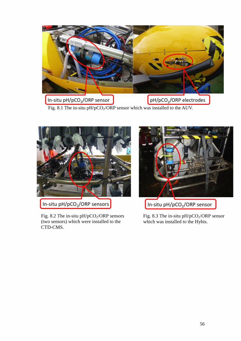
56

Fig. 8.1 The in-situ pH/pCO2/ORP sensor which was installed to the AUV.

Fig. 8.2 The in-situ pH/pCO2/ORP sensors

(two sensors) which were installed to the

CTD-CMS.

Fig. 8.3 The in-situ pH/pCO2/ORP sensor

which was installed to the Hybis.

57

Results

For example, the result in the Autosub68 mission is shown in Fig. 4. In this

mission, the AUV cruised four lines in north-south direction. The small decrease of

pH and increase of pCO2 (areas A, C, D and F) were detected in four cruising lines.

The areas of low pH and high pCO2 were in two southernmost areas (B and E), and

the pH in area B was lower 0.01pH than area E though the depth was almost same in

both areas. These results suggest that there are low pH and high pCO2 seawater near

bottom in area B and there are the slightly low pH and high pCO2 seawater area A, C,

D and F. On the other hand, the result of ORP was different from them of pH and

pCO2, because ORP respond to H2S and/or charged suspended matter, not CO2.

Fig. 8.4 The results of in-situ pH, pCO2 and ORP observation in the Autosub68

mission.

I plan to draw up detail horizontal and vertical contour maps of pH and pCO2 in

the Sleipner Site by using in-situ pH and pCO2 data that are obtained by AUV and

CTD-CMS observations for the assessment of CO2 leakage at the site.

58

Section 9. JC077 NMFSS Ship Fitted Systems

Jez Evans, Dave Childs, Rees Roberts, Tom Roberts

Gareth Knight (Science Systems Tech)

Jez Evans (Senior Tech)

Meteorology monitoring package.

The Surfmet system was run throughout the cruise. Please see the separate BODC

information sheet JC77_Surfmet_sensor_information_sheet.docx for details of the

sensors used and the calibrations that need to be applied. The calibration sheets are

included in the directory Ship_Systems\Met\SURFMET\calibrations on the final ships

data disk.

Pumped sea water sampling system [hull bottom intake]. Sea surface monitoring

system [salinity, temperature, transmissometre, fluorimetre].

The Surfmet system was run throughout the cruise. Please see the separate BODC

information sheet for details of the sensors used and the calibrations that need to be

applied. No problems were encountered. The calibration sheets are included in the

directory Ship_Systems\Met\SURFMET\calibrations on the final ships data disk.

Ship scientific computing systems.

Data was logged by the Techsas data acquisition system into NetCDF files. The

format of the NetCDF files is given in the file

NMFSS_NetCDF_Description_Cook.docx. The instruments logged are given in

JC77_Ship_fitted_information_sheet_JC.docx. Data was additionally logged into the

RVS Level-C format, which is described in the same document. Tim LeBas from

NOC Southampton processed the 710 multibeam data using his own Caris package.

The Level-C software was run on the new Sun Enterprise Sparc server. The

Enterprise does not have a monitor output and so the fromtechsas program was started

remotely and run in the background. This worked well and there were no problems

when the xterm that it was started in was closed. The Cook file server was used to

provide a network storage area which was used to provide shared storage for everyone

to use. This was copied to the end of cruise data disk.

Kongsberg EA600 12 kHZ single beam echo sounder.

The EA600 single beam echo sounder was run throughout the cruise. The results are

typical for this vessel with lots of aeration under the hull and some poor performance

from the acoustic systems in rough weather. During the cruise this could also be seen

in the EM710 multibeam and EK60 multi frequency sounder underway data. The

underway depth data logged is therefore of variable quality with lots of spikes and

gaps as a result. Before using depth data from the EA600’s NetCDF file the .bmp files

should be consulted to see if the depth data for that time period was reliable. The

EA600 was used with a constant sound velocity of 1500 ms-1

throughout the water

column to allow it to be corrected for sound velocity in post processing, though

corrections would be very minor with water depths of typically 85m.

All systems were turned off during all AUV deployments.

59

Kongsberg EM710 SHALLOW/MID Water Multi beam echo sounder.

It was also run throughout the cruise to provide general depth information.

The EM710 suffered from some poor performance due to aeration caused by the

vessel’s pitching motion, although to a slightly lesser extent than the EA600. The

drop keel was flush with the hull for the whole of the cruise as a data calibration of

the transducers was required and subsequent movement of the drop keel would have

rendered this calibration invalid.

EM710 water column data are logged within the Kongsberg raw all files during the

complete survey. This data greatly adds to the size of the raw files. It was decided that

logging in this way was the most likely to cater for all possible future post processing

requirements. As post processing requirements become clearer it may be more

convenient on future cruises to collect water column and bathymetry data into

separate files, this would certainly make the processing of the bathymetry quicker.

Olex was run throughout the cruise and was useful for identifying sites to sample at

and the location of the vessel relative to the next station.

Sound Velocity Profiles.

The sound velocity profile data are included on the data disk from CTD casts.

75 kHz and 150 kHz hull mounted ADCP system.

Neither was run on the cruise as considerable compromise with the EK60 and EM710

data logging rate would have been required. Also some acoustic interference would

have been inevitable.

Wave height recorders.

The antenna unit for the Wamos wave radar was run for part of the cruise for test and

calibration purposes and the data collected included on the final data disk in the

WAMOS directory.

CTD.

The CTD data is included on the data disk in Specific Equipment\CTD\.

EK60

EK60 data was collected throughout the cruise and the system setup with a two

second ping rate and pulse length of 1024 uS and sample length of 256 uS. The

recommended/default power settings for the transducers were used.

Transducers frequencies of 18Khz, 38Khz, 120Khz and 200Khz were recorded. The

70Khz transducer was not run as previous experience on past cruises had shown that

data from the EM710 water column was significantly degraded when both these

instruments operate at the same frequency.

60

Section 10. Summary and Conclusions.

The cruise was a great success and demonstrated the ability to perform large aerial

surveys over relatively short time periods. These surveys were complemented with a

water sediment sampling programme where targets were located using the on-board

and AUV sensor systems. We completed over 1300 km of survey lines and produced

high quality multibeam maps that covered 246 km2 of seafloor. The chemical sensors

on both the AUV, CTD and Hybis revealed areas enriched with methane and reduced

species. The work will continue on the samples back at NOC.

61

Appendix 1

Instructions for Autosub 6000 Edgetech data processing

1. Data appears as a series of DAT000xxx.jsf files these need to be converted to

XTF format using the Discover 4200 MP 2.03 program.

2. Click the Configuration....Record menu item and tick the XTF Output box

3. On the tabs at the bottom click the Disk tab. On this set the

record file directory to where you wish the xtf files to be

kept.

4. Before recording the xtf files the video gains will need to be set. Choose one

jsf file for playback, set it playing and possibly increasing speed using the

button. Then select the VideoGains tab and hit Normalise. This will set an

instantaneous gain levels for Gain and TVG. Average setting is Gain 29dB

and TVG 18dB/100M but look at imagery to confirm.

5. Back to the Disk Tab. Select a Playback file and as soon as it starts hit the

record button . Speed the process up by using the button - max speed is

20.

6. Proceed through all the jsf files in order, waiting for each to finish after a

initial speed up. This is slow and laborious. Ignore the Data written tally, each

xtf file has a maximum size of about 280Mb. It will also create new jsf files -

these can be deleted.

7. Once finished all the DAT000xxx.jsf files then move to PRISM.

8. Create directories and sub-directories for the cruise, autosub and the mission

name and cdf. e.g. /home/tlb/JC77/autosub/m59/cdf and another

directory for nav

e.g. /home/tlb/JC77/autosub/m59/nav

9. In the cdf directory make a file listing all the high frequency (or low but not

both) xtf files on the windows disk. e.g

ls /cdrive/Users/tlb/Documents/JC77/autosub/m59/xtf/*H.xtf >

highlist

10. In the same directory use the loopfile command to convert all the xtf files to

Netcdf format. Sub-sampling is suggested as the data across track is of

considerably higher resolution across track than along-track. Example: On JC77

the HF data was 1.2cm resolution by 29.7cm ping spacing.

e.g. loopfile reson2prism m59 highlist cdf 1 -z 31 -a 4400 -f 5

The parameters are:

a. reson2prism - conversion programme

b. m59 - mission number

c. highlist - list of xtf files (including pathname)

d. cdf - output datatype

62

e. 1 - starting pass number

f. -z 31 - UTM zone 31

g. -a 4400 - Number of samples in output file (22160 on input)

h. -f 5 - Sub-sampling factor of input imagery

11. A separate navigation file should be available from the Autosub team. This is

a ASCII text file with columned data: Mission, Date, Time, Lat, Long, Head,

Roll, Pitch, Depth, Altitude

12. Put this file in the nav directory and edit it and remove the headings wording

(first line) and then save as a nav file e.g. m59.nav

13. Run wireout to produce a veh_nav file . Zero cable out value and Zero added

minutes and weight is immaterial.

14. Create a commands.cfg file for the type of sidescan data. For example high

frequency sidescan:

addnav -i %1 -o %0 -s 1.0

widealt -i %1 -o %0 -p

mrgnav_inertia -i %1 -o %0 -u 0 -r 0.0,0.0 -n navfile.veh_nav

edge16 -i %1 -o %0 -m

shade_tobi -i %1 -o %0 -n 1000

tobslr -i %1 -o %0 -r0.0576 , res # high freq 110m 6 Hz subsamp 5

filter -i %1 -o %0 -b 1,351 -h -v 1,5000

filter -i %2 -o %0 -b 21,351 -l -v 1,5000

wtcombo -i %2 , %1 -o %0 -c 1,1

restorehdr_tobi -i %1 -h %5

widealt -i %2 -o %0 -h -l 500

15. Go to the cdf directory and choose a sample middle cdf file and draw a profile

across track of the pixel values on one line to find a threshold value from

background water column to first return.

e.g. profile m59p20.cdf 100

The parameters are:

a. m59p20.cdf - chosen file

b. 100 - line number

Example: Value of 250 if peaking at 1000 and background is 0-40.

16. Test the files for time continuity

e.g. do_test_times m59 1 63 0.2

The parameters are:

a. m59 - mission name

b. 1 - first pass number

c. 63 - last pass number

d. 0.2 - pulse repetition rate

If time jumps (backward) use dk2dk_tobi to divide up the files

17. Create an .index file for all the cdf files

e.g. do_create_index m59 1 63

If the m59.index has conflicts of time these must be solved before continuing.

It may useful to copy the index file to the main directory.

63

18. The data has no altitude values and these must be calculated from the first

return.

e.g. do_alt_index m59.index 250 13.2 normal 1 n

The parameters are:

a. The name of the index file to run (e.g. m59.index)

b. Threshold of water column (e.g. 250)

c. The starting altitude (e.g. 13.2m)

d. Type of Bottom (rocky, default, normal or smooth)

e. Speed of detection (default 10 times) 1 is best

f. View results (default is y) for checking

g. Any options you require (e.g. -t -m 10)

-n use starboard side only on altimetre correction

-t use port side only on altimetre correction

-m clean water column for given value depth in metres

19. The altitude values are in .cdfnew files and need to be renamed to .cdf

e.g. renaming cdfnew cdf

20. In the main directory the data is now ready to run maptile to produce the tile

areas.

21. Finally run prism5 in the main directory, insert the correct parameters and run

all maps

64

Appendix 2: Summary of JC77 HyBIS Dive Logs

JC77 Station no. Dive no. Start of

Dive End of Dive Comments

JC77-5-185 124 259/1956 259/2131 Grab sample taken at 2109, Downward camera back to front

JC77-5-203 125 260/1830 260/1955 Grab sample taken at 1938, EH-sensor attached to the front of the vehicle

126 260/2027 260/2048 Dive abandoned due to camera malfunction

JC77-5-204 127 260/2100 260/2201 Grab sample taken at 2142

JC77-2-222 128 261/2000 261/2121 EH-sensor attached to the front of the vehicle





