jorge caralhov costa - biblioteca digital de teses e ... · pdf filejorge caralhov costa ... a...
TRANSCRIPT

JORGE CARVALHO COSTA
ESSENTIAL BOUNDARY AND INTERFACE CONDITIONS IN THE
MESHLESS ANALYSIS OF SHELLS
São Paulo
2015

JORGE CARVALHO COSTA
ESSENTIAL BOUNDARY AND INTERFACE CONDITIONS IN THE
MESHLESS ANALYSIS OF SHELLS
Thesis submitted to the Polytechnic School at
the University of São Paulo for award of the
Doctor of Science Degree.
São Paulo
2015

JORGE CARVALHO COSTA
ESSENTIAL BOUNDARY AND INTERFACE CONDITIONS IN THE
MESHLESS ANALYSIS OF SHELLS
Thesis submitted to the Polytechnic School at
the University of São Paulo for award the
Doctor of Science Degree.
Area: Structural Engineering
Advisor: Prof. Dr.Paulo de Mattos Pimenta
São Paulo
2015

Catalogação-na-publicação
Costa, Jorge Essential boundary and interface conditions in the meshless analysis ofshells / J. Costa -- São Paulo, 2015. 63 p.
Tese (Doutorado) - Escola Politécnica da Universidade de São Paulo.Departamento de Engenharia de Estruturas e Geotécnica.
1.shells 2.meshless methods 3.nitsche's method 4.multi-region problems5.shear deformable shells I.Universidade de São Paulo. Escola Politécnica.Departamento de Engenharia de Estruturas e Geotécnica II.t.

Essential boundary and interface conditions in themeshless analysis of shells
Esta é a versão original da tese elaborada pelo
candidato Jorge Carvalho Costa, tal como
submetida à Comissão Julgadora.

Acknowledgments
Firstly, I would like to thank Prof. Paulo Pimenta for taking me as a student and
guiding me through my research and more importantly through a real academic formation.
Thank you for the many fruitfull and happy get-togethers and conversations, about my
research and a whole variaty of other subjects. It has been an honor to be your student.
Other masters were also kind enough to advise and help me, especially Prof. Carlos
Tiago who welcomed me for a stay in Lisbon during my masters and became my referrence
for all matters of meshless methods, and Prof. Eduardo Campello for great insights and
helpful discussions.
My sincere gratitute to Prof. Peter Wriggers for receiving me at the Institut für Kon-
tinuumsmechanik in Hannover for a prolic and very pleasant year. Thank you for helping
my research and formation.
To my co-workers and oce mates, thank you for providing a nice working environ-
ment, for attentive ears to obstacles and smily faces for the happy-hours. It was my priv-
ilege to work with Eduardo Simões, Paulo Nigro, Fernando Gonçalves, Marco Sampaio,
Henrique Gomes, Leonardo Lago, Marcelo Teixeira, Igor Pierin, Nadia Ota, Alfredo Gay
Neto, Márcia Sato, Alexandre Belleti, Luís Bitencourt, Ricardo Lahuerta at University of
São Paulo, and to know some of their delightful families.
I also thank the new friends I made in Hannover, who made me feel welcome so
far from home: Ajay Harish, Mohamed Anndif, Mohammadreza Hojjati, Sebastian Zeller,
Saleh Yazdani, Vinh Hiep, Tobias Steiner and Christian Weiÿenfels among others at IKM.
Also to Mrs. Halfar and Mrs. Schulte for all the help.
I was also lucky to nd in Germany great new friends outside of the workplace. I
thank Carlos Lopes, Melanie Titz and her many friends, Irene di Palma, Robin Corgier
and Gabriela Szafarska, great atmates, Mr. and Mrs. Franke. My best appreciation Rita
Castro, Lüder Meyer and the Meyer family for such a great hospitality and also to the
loving Totzke family.
My acknowledgment also go to CNPq (Conselho Nacional de Desenvolvimento Tec-
nológico) for a PhD scholarship and CAPES (Coordenação de Aperfeiçoamento de Pessoal
de Nível Superior) for supporting my exchange stay at IKM with grant BEX 14618/13-3.
i

Agradecimentos
É com um imenso prazer que agradeço a todos aqueles que caminharam junto comigo
nessa jornada. Agradeço a Deus pelas oportunidades que me dá, pela minha paz e pelas
pessoas que coloca junto a mim.
Agradeço a minha família por me dar segurança que o amor é grande e não conhece
distâncias. A minhas avós Iza e Inês por todo carinho e por sempre rezarem por mim,
as avós emprestadas Eunice e Nazinha por engrossarem esse coro, a meus avôs Joaldo
e Lealdo (ambos in memorian) pelas recordaçoes e lições e também ao avô emprestado
Osvaldo pelo carinho e as conversas sempre interessantes.
Dedico muito carinho a meus Tios e Tias que me guiam e suportam sempre. Em
especial a minhas sempre presentes tias-mães Tereza e Marly, Rosa e Ângela; e tia Vânia,
companheira de doutorado, que me incentiva e guia para a vida acadêmica, obrigado pela
conança. A meus tios João, Joca, Bôsco, Ricardo e Ivo por serem grandes exemplos. A
meus primos-irmãos Joaldo, Evelyne e Izinha pelo apoio, companhia e amizade verdadeira.
A meus primos-alhados Vítor, Matheus, Rodrigo, Eduardo, Geovana e Thainá, que já
cresceram, enjoaram das brincadeiras sem graça e se tornaram companheiros. A Jaiane e
Léo, meus novos primos, e a Júlia por seu carinho sincero.
Também agradeço a minha família de Dores pela atenção e afeto, em espcial a Thiago
pela torcida e apoio. Tudo que puder fazer por minha familia é pouco diante do que
representa a mim.
Agradeço aos amigos que espalhei por aí e que me fazem sentir bem em todo lugar. A
Alexandre, Anne, Walter e Íris pela paciência no dia a dia de quem mora junto. A Ryan,
Moacir, Carlinhos, Yuri, Heloisa, Fabiana, Rodrigo Cocate e outras guras paulistanas.
A Ariel, Marcelinho, Aloísio, Samuel, Higor Sérgio, Marcel, Anísia, Thaísa, Gustavo, Ju-
liana, Rony, Jorge, Fábio, Lucas, Diogo, Gugu, Madson, Flávio, Plínio e Ícaro. A Carlão
Hermínio, Vítor e os outros 30 e tantos primos e tios.
Por m, meu maior agradecimento a meus pais: Jorge Lima e Luzia. Obrigado pelo
suporte, apoio, torcida, carinho e todas as formas de bem que sempre dirigiram a mim.
Dedico esse trabalho a vocês.
ii

Resumo
Costa, J. C. . Condições essenciais de contorno e interface na análise de cas-
cas com métodos sem malha. 2015. 63 f. Tese (Doutorado) - Escola Politécnica da
Universidade de São Paulo, São Paulo, 2015.
Métodos sem malha geram campos de aproximação com alta continuidade, conve-
nientes para estruturas nas como cascas. No entanto, a ausência da propriedade de Delta
de Kronecker diculta a formulação de condições essenciais de contorno, já que os campos
de aproximação e teste não podem ser moldados aos valores de contorno. Um problema
similar aparece quando diferentes regiões de aproximação precisam ser juntadas em um
problema multi-regiões como dobras, vincos ou junções. Este trabalho apresenta três méto-
dos de imposição ambas condições cinemáticas: o já conhecido método dos multiplicadores
de Lagrange, usado desde o começo do método de Galekin sem elementos (EFG); uma
abordagem de penalidade pura; e o recentemente redescoberto método de Nitsche. Nós
usamos a técnica de discretização com EFG para cascas espessas de Reissner-Mindlin e
adaptamos a forma fraca de forma a separar graus de liberdade de deslocamento e rotação
e obter coecientes de estabilização diferentes e apropriados. Essa abordagem permite a
modelagem de cascas discontínuas e o renamento local em problemas multi-regiões.
Palavras-chave: cascas, métodos sem malha, método de Nitsche, problemas multi-regiões,
cascas com cisalhamento.
iii

Abstract
Costa, J. C. . Essential boundary and interface conditions in the meshless anal-
ysis of shells. 2015. 63 p. Thesis (Doctorate) - Escola Politécnica da Universidade de
São Paulo, São Paulo, 2015.
Meshless methods provide a highly continuous approximation eld, convenient for thin
structures like shells. Nevertheless, the lack of Kronecker Delta property makes the for-
mulation of essential boundary conditions not straightforward, as the trial and test elds
cannot be tailored to boundary values. Similar problem arise when dierent approxima-
tion regions must be joined, in a multi-region problem, such as kinks, folds or joints. This
work presents three approaches to impose both kinematic conditions: the well known La-
grange Multiplier method, used since the beginning of the Element Free Galerkin method;
a pure penalty approach; and the recently rediscovered alternative of Nitsche's Method.
We use the EFG discretization technique for thick Reissner-Mindlin shells and adapt
the weak form as to separate displacement and rotational degrees of freedom and obtain
suitable and separate stabilization parameters. This approach enables the modeling of
discontinuous shells and local renement on multi-region problems.
Keywords: shells, meshless methods, nitsche's method, multi-region problems, shear de-
formable shells.
iv

... and I have my mind ...
and a mind needs books as a sword
needs a whetstone, if it is to keep its edge
- George R. R. Martin

Contents
1 Introduction 1
2 Linear shell theory 4
2.1 Introduction . . . . . . . . . . . . . . . . . . . . . . . . . . . . . . . . . . . 4
2.2 Kinematics . . . . . . . . . . . . . . . . . . . . . . . . . . . . . . . . . . . 4
2.3 Statics . . . . . . . . . . . . . . . . . . . . . . . . . . . . . . . . . . . . . . 8
2.4 Linear approximation . . . . . . . . . . . . . . . . . . . . . . . . . . . . . . 10
2.5 Material . . . . . . . . . . . . . . . . . . . . . . . . . . . . . . . . . . . . . 11
2.6 Initial Deformation . . . . . . . . . . . . . . . . . . . . . . . . . . . . . . . 12
2.7 Weak Form of Equilibrium . . . . . . . . . . . . . . . . . . . . . . . . . . . 13
2.8 Multi-region shells . . . . . . . . . . . . . . . . . . . . . . . . . . . . . . . 14
3 Meshless Approximation 16
4 Kinematic Constraints 20
4.1 Lagrange Multipliers . . . . . . . . . . . . . . . . . . . . . . . . . . . . . . 22
4.2 Penalty Method . . . . . . . . . . . . . . . . . . . . . . . . . . . . . . . . . 27
4.3 Nitsche's Method . . . . . . . . . . . . . . . . . . . . . . . . . . . . . . . . 31
5 Numerical Examples 41
5.1 Stabilization for EBCs . . . . . . . . . . . . . . . . . . . . . . . . . . . . . 41
5.1.1 Displacement DOFs . . . . . . . . . . . . . . . . . . . . . . . . . . . 41
5.1.2 Rotation DOFs . . . . . . . . . . . . . . . . . . . . . . . . . . . . . 43
5.2 Stabilization for Interfaces . . . . . . . . . . . . . . . . . . . . . . . . . . . 45
5.2.1 Displacement DOFs . . . . . . . . . . . . . . . . . . . . . . . . . . . 45
5.2.2 Rotation DOFs . . . . . . . . . . . . . . . . . . . . . . . . . . . . . 47
5.3 Pinched Cylinder . . . . . . . . . . . . . . . . . . . . . . . . . . . . . . . . 49
5.4 T-beam . . . . . . . . . . . . . . . . . . . . . . . . . . . . . . . . . . . . . 51
6 Conclusions 56
vi

Chapter 1
Introduction
Meshless approximations provide a great resource for the analysis of structures as
high order continuity in the approximated elds can be achieved. This feature is well
suited for thin systems like shells, provided that the geometry can be better approximated
and stresses can be obtained as smoothly as desired. They have been applied to thin
Kirchho-Love shells [37, 31], where C1 continuity is necessary, moderately thick Reissner-
Mindlin shells [48, 58, 12] and solid-like shells based on 3D continuum [38]. However, the
non-interpolatory characteristic of such approximants makes the formulation of essential
boundary and interface conditions not straightforward.
We introduce interface conditions for continuity and equilibrium across a boundary
between two discretization domains. The coupling of multiple regions is quite straight-
forward in Finite Elements (FE) with matching nodes along the interface, but this limits
the liberty of each region's renement. A growing application in Computer Aided En-
gineering is the possibility to analyze full, complex models composed of multiple parts,
keeping the possibility to rene the response in most critical areas. In Computational
Mechanics, this translates into the need for multiple regions to be describe together while
maintaining the ability to be rened independently. One region might possibly need a
more rened solution, or dierent approximation techniques might be employed in each
side of the interface (i.e., FEs and meshless). Similar problem arise when dealing with
approximations that do not fulll the Kronecker delta property such as most meshless
methods (meshless approximations on both domains). For mapped shell theories, each
domain must also be smooth, so any kink or junction of shells is treated as a interface
between independently approximated elds.
Essential boundary conditions (EBCs) and interface conditions (ICs) are formulated in
the same way and have been discussed since the early development of meshless methods.
From the beginning, as in the classical Element-Free Galerkin Method (EFG, [6]), La-
grange Multipliers have been used to enforce EBCs, but disadvantages like increasing the
number of unknowns for the problem and limitations on the choice of approximation elds
compelled more research on the subject [35, 18]. Solutions ranged from coupling with FEs
1

1. Introduction 2
along the boundaries [7, 29] to the use of the domain shape functions to approximate the
Lagrange multipliers [42, 43, 9].
Recently, an alternative has been revisited: the interior penalty method, usually re-
ferred to as Nitsche's Method [47], which identies the Lagrange Multipliers with the ux
at the essential or interface boundary and introduces a penalty-like stabilization param-
eter, which guarantees the coercivity of the bilinear form.
Among other applications, this approach has been used to impose EBCs in Poisson's
problems with meshless methods [20, 18] and FEs [57]. It has been applied with eXtended
Finite Elements (XFEM) for EBCs and ICs in single-eld problems [15, 25, 28], to enforce
weak discontinuities between elastic materials [51, 52, 2, 1]; and applied to non conforming
embedded FE meshes for elastostatics [53, 54]. B-splines and NURBs-base FEs share
similar features with meshless approximations and can also take advantage of Nitsche's
Method, as in [16] for 2nd and 4th order problems, [46, 33, 49, 50] for elasticity, [27, 26]
for thin plates and [22, 23] for thin shells. The theory has also been extended for contact
with FEs [59] and XFEM [4, 3].
It is the authors' opinion that in the future Nitsche's method may become the
standard treatment to enforcing essential boundary condition for meshfree
Galerkin methods. [39, p. 114]
The present work develops Nitsche's method for the linear elastic analysis of shear de-
formable Reissner-Mindlin shells [12], both for the imposition of boundary displacements
and for multi-region problems. In the latter, renement over one portion of the domain
can be performed without aecting other regions, even maintaining their stiness matri-
ces, and dierent regions can be discretized with dierent approximants, e.g., FE-EFG or
EFG-IGA coupling.
In both cases, its advantage over Lagrange Multipliers is that it precludes the deni-
tion of a new approximation space, new degrees of freedom and a hybrid interpolation,
along with its complications. A penalty-like stabilization term is necessary to ensure the
coercivity of the bilinear form. Nevertheless, the weak form remains consistent and, con-
trary to a pure penalty imposition, accuracy is guaranteed for a wide range of values for
the parameter.
The shear deformable shell theory is developed in [14] with Finite Elements and in
[58] with Multiple Fixed Least Squares (MFLS). In [12], a consistent linear model is de-
rived for small displacements and rotations, using MFLS and Lagrange multipliers. The
extension to geometrically exact thin shells is present in [31] and the boundary conditions
are discussed in [32]. This work presents the multi-region formulation for independent
particle distributions, using both Lagrange multipliers and Interior Penalty for the inter-
faces. Numerical examples are laid out to assess the method's suitability, while comparing
solutions with similar number of degrees of freedom.

1. Introduction 3
Throughout the text, italic Greek or Latin lowercase letters (a, b, ... , α, β, ...) de-
note scalar quantities; bold italic Greek or Latin lowercase letters (a , b, ... , α, β, ...)
denote vectors and bold italic Greek or Latin capital letters (A, B , ... , Φ, Γ , ...) denote
second-order tensors in a three-dimensional Euclidean space. Summation convention over
repeated indices is adopted, with Greek indices ranging from 1 to 2 and Latin indices
from 1 to 3.

Chapter 2
Linear shell theory
2.1 Introduction
The nonlinear shell theory developed in [14] has been later remodeled in a consistent
way to a neat linear formulation in [12] to the rst order in the displacements and rotations.
This chapter outlines the process as in [10] so a consistent linear shell model is obtained.
The shell is parameterized by a at reference conguration, consisting of a at midsur-
face and a thickness h. The initial curved conguration is then obtained by a stress-free
transformation after which the actual or eective transformation takes place. Fig. 2.1
depicts these transformations for the geometrically exact shell.
Let e i be an orthogonal frame, with the vectors erα on the reference plane and the
vector er3 orthogonal to it. At the reference conguration, a point of the shell can be
described by its position
ξ = ζ + ar, (2.1)
where ζ = ξαerα denes the projection of this position in the midsurface and ar = ξ3er3
is the through-the-thickness component. The set [ξ1, ξ2, ξ3] denes a Cartesian system of
coordinates in three dimensions.
The shell's midsurface is the domain Ωr ∈ er1×er2 and we assume that the midsurface
is actually on the midpoint of the shell thickness ξ3 ∈ [−h/2,h/2]
2.2 Kinematics
The initial deformation is regarded as a mapping from the at reference conguration.
The position of the shell midsurface points is described in its initial stress-free congura-
tion by
z o = z o (ξα) . (2.2)
4

2. Linear shell theory 5
O reference configuration
er
3
er
1
er
2
ar
initialconfiguration
eo
1
eo
2
eo
3ao
currentconfiguration
e1
e2
e3
a
zo
xo
z
x
u
Figure 2.1: Shell kinematics for large displacements
These displacements are nite, and so are the rotations of the midsurface and the
director. Nevertheless, Kirchho-Love kinematics is assumed, so that the director ao re-
mains normal to the curved midsurface. We can describe this rotation by the tensor Qo
so
ao = Qoar = Qoξ3er3. (2.3)
The reference frame follows the same rotation,
eoi = Qoeri , (2.4)
what makes it describable by
Qo = eoi ⊗ eri (2.5)
As the initial frame eoi follows the midsurface curvature, it can be expressed of the
derivatives of the initial position by the mapping coordinates:
eo1 =z o,1‖z o,1‖
, (2.6a)
eo2 = eo3 × eo1 and (2.6b)
eo3 =z o,1 × z o,2‖z o,1 × z o,2‖
. (2.6c)
eo1 and eo2 are tangent to the shell surface and the director is ao = ξ3eo3. With the

2. Linear shell theory 6
denition of the initial cross-sectional strain vectors
ηoα = z oα −Qoerα and (2.7a)
κoα = axial(Qo
,αQoT),K o
α = Skew (κoα) (2.7b)
at hand, the initial strain vectors at any material point can be computed by
γoα = ηoα + κoα × ao, (2.8)
so that the initial deformation gradient can be expressed by
F o = (ηoα + K oαao)⊗ erα + Qo = γoα ⊗ erα + Qo. (2.9)
The quantities above are aected by superposed rigid body motions and not suit-
able for an objective theory. Therefore, it's compelling to introduce their back-rotated
counterparts as follows
γorα = QoTγoα = ηorα + κorα × ar (2.10a)
ηorα = QoTηoα = QoTz o,α − erα (2.10b)
κorα = QoTκoα =(eo2,α · ee3
)er1 +
(eo3,α · ee1
)er2 +
(eo1,α · ee2
)er3 (2.10c)
F or = QoTF o (2.10d)
For later use, it is convenient to gather the initial cross-sectional strain vectors in two
generalized initial strain vectors
εorα =
[ηorα
κorα
]. (2.11)
Next, the actual motion of the shell takes place. The displacement of any point in the
shell can be once again split into the displacement u of its projection on the midsurface
and a rotation of the director a = Qeao. Since Reissner-Mindlin kinematics is assumed,
the cross-section rotation is considered an independent quantity. The eective rotation θ
can be described by Euler parameters grouped in the rotation vector through the Euler-
Rodrigues relation:
Qe = I + h1 (θ) Θ + h2 (θ) Θ2, (2.12)

2. Linear shell theory 7
where
Θ = Skew (θ) , (2.13a)
θ = ‖θ‖, (2.13b)
h1 (θ) =sin (θ)
θ, (2.13c)
h2 (θ) =1
2
(sin(θ2
)θ2
)2
. (2.13d)
The current position of a material shell point can be expressed by
x = z + a = z o + u + Qeao. (2.14)
The components of u along with the components of θ in a global Cartesian system
dene the six degrees of freedom of the theory.
The deformation from the at reference conguration to the current deformed cong-
uration is called the total deformation, and its gradient is given by
F =∂x
∂ξ= Q + (ηα + κα × a)⊗ erα (2.15)
where, as it was done for the initial deformation, one can dene
ηα = z ,α − eα = z o,α + u ,α −Qerα and
κα = axial(Q ,αQT
)= κeα + Qeκoα,
(2.16)
as the cross-sectional strain vectors. Once again, their back-rotated counterparts are more
suitable for an objective theory. After some algebra, we arrive at
ηrα = QTηα = QTz ,α − erα and
κrα = QTκα = κerα + κorα ,(2.17)
whereκerα = Γ Tθ,α, with
Γ = I + h2 (θ) Θ + h3 (θ) Θ2 and
h3 (θ) =1− h1 (θ)
θ2.
(2.18)
Finally the back-rotated strain vectors can be dened as
εrα =
[ηrα
κrα
], (2.19)

2. Linear shell theory 8
and the total back-rotated strains as
γrα = ηrα + κrα × ar, (2.20)
so the total deformation gradient can be expressed by
F = Q (I + γrα ⊗ erα) . (2.21)
Its back-rotated counterpart, not aected by rigid body motions is
F r = QTF = I + γrα ⊗ erα (2.22)
This total deformation gradient can be decomposed into initial and eective ones
F = F eF o,F e = FF o−1 = Q (f eri ⊗ eoi ) . (2.23)
The eective back-rotated strains can be dened as
γerα = f erα − erα = Jo−1(erα · g orβ
) (erβ + γrβ
)− erα, (2.24)
where g orβ are derived from the initial transformation and Jo is its Jacobian, as follows
Jo = detF o = detF o = er3 · f or1 × f or2 , (2.25a)
g or1 = f or2 × er3, gor2 = er3 × f or1 , g
or3 = f or1 × f or2 . (2.25b)
2.3 Statics
The shell specic internal power per unit volume at the reference conguration can be
expressed by
P : F = JoP : Fe
= τ rα · ηrα + (ar × τ rα) · κrα, (2.26)
where P = τα ⊗ erα is the rst Piolla-Kirchho stress tensor, τ rα = QoTτα are its back-
rotated column vectors and F is the velocity gradient. Integration across the thickness
yields the internal power per unit area of the midsurface in the initial conguration∫H
(P : F
)dH = nr
α · ηrα + mrα · κrα, (2.27)
where H = [−h/2,h/2] is the thickness domain and the vectors
nrα =
∫H
(τ rα) dH and mrα =
∫H
(ar × τα) dH (2.28)

2. Linear shell theory 9
are the back-rotated force and moment resultants, respectively. Those can be gathered in
the generalized back-rotated stress vectors
σrα =
[nrα
mrα
](2.29)
so that the internal the internal power of the shell is
P int =
∫V r
(P : F
)dV r =
∫Ωr
(σrα · εrα) dΩr. (2.30)
The external power can be computed in the reference conguration by
P ext =
∫Ωr
(qΩ
r · d)dΩr +
∫Γ rt
(qΓ
rt · d
)dΓt +
∫Γ ru
(qΓ
ru · d
)dΓ r
u (2.31)
where
qΩr
=
[nΩr
Γ TmΩr
](2.32)
are the force and moment resultants of the loads applied in the domain,
qΓrt =
[nΓ rt
Γ TmΓ rt
](2.33)
in the natural boundary and
qΓru =
[nΓ ru
Γ TmΓ ru
](2.34)
are the (unknown) reactions in the essential boundary Γ ru . Those (true) stress resultants
are dened as
nΩr = ttr
+ tbr
+
∫h
brdh
mΩr = a × tbr
+
∫h
a × brdh
(2.35a)
on the domain,
nΓ rt =
∫h
tlrdh
mΓ rt =
∫h
a × tlrdh
(2.35b)

2. Linear shell theory 10
on the Neumann boundary, and
nΓ ru =
∫h
rdh
mΓ ru =
∫h
a × rdh
(2.35c)
on the Dirichlet boundary.
In (2.35), tt, t
b, tl are, respectively, the external surface tractions on the top, the
bottom and the lateral of the shell, per unit reference area, b is the body force vector
per unit reference volume and r is the reaction on the lateral surface at the kinematic
boundary.
2.4 Linear approximation
The consistent linearization of the model to a rst order in the displacements and
rotations was carried out in [12]. The obtained model is similar to a thick plate theory,
encompassing shell curvature and membrane deformation.
To the rst order in θ, the displacement δ during the eective transformation of a
given point in the shell is
δ = u + θ × ao. (2.36)
Back-rotated (objective) generalized membrane and curvature strain quantities [8, p.
2043] can be dened as the approximations of Eq. 2.17 to the rst order in u and θ
ηrα = QoT(z o,α + Z o
,αθ + u ,α
)− erα and (2.37a)
κrα = QoT(κo,α + θ,α
). (2.37b)
where
Z o,α = Skew
(z o,α). (2.38)
It is interesting to note the neat additive property
ηrα = ηorα + ηer, where (2.39a)
ηorα = QoTz o,α − erα and (2.39b)
ηerα = QoTZ o,αθ + QoTu ,α (2.39c)
and
κrα = κorα + κer, where (2.40a)
κorα = QoTκoα =(eo2,α · eo3
)er1 +
(eo3,α · eo1
)er2 +
(eo1,α · eo2
)er3 (2.40b)

2. Linear shell theory 11
κerα = QoTθ,α, (2.40c)
of the generalized strains. It's also compelling to split the generalized strain vectors εrαgiven in (2.19) into initial and eective strains
εrα = εorα + εerα . (2.41)
The initial strains εorα are given by (2.39b) and (2.40b) and εerα can be expressed in
matrix for as
εerα = ∆αd , (2.42a)
∆α =
[QoT 0
0 QoT
][I ∂∂ξα
Z o,α
0 I ∂∂ξα
], (2.42b)
where the shell's degrees of freedom are collected in
d =
[u
θ
]. (2.43)
2.5 Material
A generalized Hooke material is used. With the little abuse of nomenclature made
in most of the consulted literature, the model presented here is said to be subject to a
plane stress assumption. Actually, the model accounts for shear stresses in the thickness
direction, what by itself is a violation of the plane stress condition. The assumption made
herein is that there is no normal stress acting on the midsurface plane (er3 ·P rer3 = 0), as
it has been done in [13] for the polyconvex neo-Hookean Simo-Ciarlet material (see [55],
page 258). Thus, it is stated that
τ erα = C erαβγ
erβ , where (2.44a)
C erαβ =
E
2 (1− ν)erα ⊗ erβ +
E
2 (1 + ν)εαβE
r3 +
E
2 (1 + ν)δαβI , (2.44b)
which is the isotropic plane stress generalized Hooke's law in our notation. In (2.44b), the
skew-symmetric tensor E r3 = Skew (er3), the Kronecker symbol δαβ and the permutation
symbol εαβ = erα · erβ × er3 have been introduced. The linear elastic relation between
the generalized back-rotated stresses σrα and the generalized eective strains εerα can be
written as displayed below.
σrα = Dαβεerβ = Dαβ
(εrβ − εorβ
), (2.45)

2. Linear shell theory 12
er
2
er
3
er
1
eo
1e
o
2
eo
3
x1
x2
(a)
er
2
er
3
er
1
eo
2
eo
1
eo
3
x1
x2
r
(b)
er
2
er
3
er
1
eo
2
eo
1
eo
3
x1
x2
(c)
Figure 2.2: Initial deformations (a) at shell, (b) cylindrical shell and (c) spherical shell
where
Dαβ =
[Dηη
αβ Dηκαβ
Dκηαβ Dκκ
αβ
], (2.46)
with
Dηηαβ =
∫H
1
Jo(g orα · erδ) C er
δγ
(erγ · g orβ
)dξ3,
Dηκαβ = −
∫H
1
Jo(g orα · erδ) C er
δγ
(erγ · g orβ
)Ardξ3
= DκηTαβ and
Dκκαβ =
∫H
1
JoAr (g orα · erδ) C er
δγ
(erγ · g orβ
)Ardξ3.
(2.47)
In (2.47) the skew symmetric tensor Ar3 = Skew (ar) has been introduced and g orα
are the column vectors of the inverse of the transformation gradient F ori ⊗ eri given in
Eq. 2.25b.
2.6 Initial Deformation
The evaluation of the through the thickness integrals in the material matrix can be
numerically performed for any initial mapping, including parametric approximations such
as NURBS or T-splines. This can be avoided for some initial shell shapes through an
analytical evaluation. Some of the obtained expressions can be further simplied if a
thinness assumption is introduced, which is here dened by the condition hR 1 , i.e. the
initial curvature radius R of the shell is much bigger than its thickness h. In [12], those
integrations are done for the plane, cylindrical and spherical initial shapes depicted in
Fig. 2.2. The resulting expressions for the sub-matrices in (2.47), common to all explicit

2. Linear shell theory 13
and numerical mappings are
Dηηαβ = hJo−1 (g orα · erδ)
(erγ · g orβ
)C er
δγ,
Dηκαβ = DκηT
αβ = 0 and
Dκκαβ = −h
3
12Jo−1 (g orα · erδ)
(erγ · g orβ
)E r
3CerδγE
r3,
(2.48)
with Jo and g orα evaluated on the shell midsurface.
2.7 Weak Form of Equilibrium
Equilibrium can be asserted in a weak form as stating that the dierence between
internal and external works is zero. We can derive the internal virtual work from (2.30)
as
δW int =
∫Γ ru
σrα · δεrα dΩr. (2.49)
From the external power (2.31), we separate the contributions of the external loads
into the external virtual work
δW ext =
∫Ωr
qΩr · δd dΩr +
∫Γ rt
qΓrt · δd dΓ r
t (2.50)
and the external virtual work of the reaction forces
δW rea =
∫Γ ru
qΓru · δd dΓ r
u . (2.51)
That separation will come in handy when describing the imposition of essential bound-
ary conditions. Equilibrium can than be stated in a weak form as
δW reg = δW int − δW ext − δW rea = 0. (2.52)
Or in a more expressive way as nd d ∈H 1 (Ω) such that d = d in Γd and
δW reg =
∫Ωrσrα · δεrαdΩr −
∫Ωr
qΩr · δddΩr
−∫Γ rt
qΓrt · δddΓ r
t −∫Γ ru
qΓru · δddΓ r
u = 0(2.53)
for all δd ∈H 1 (Ω). It is important to note that using a non-interpolatory approximation
δd cannot be made to vanish on the essential boundary, thus the last term (in Γ ru) is not
canceled like in a Finite Element framework.
This imposition is linear on the generalized displacements as the stresses σrα are linearly
dependent on the strains εrα according to (2.45) and δεrα = ∆αδd is the variation of (2.41)

2. Linear shell theory 14
o
4F
r
4W
o
4W
r
u4G
o
u4G
o
i4Go
t4G
r
t4G
r
i4G
o
1W
o
2W
o
3W
o
W
r
2W
o
t1G
o
u1G
o
uG
o
tG
o
1F
o
2F
o
3F
r
1W
r
t1G
o
t2G
r
t2G
r
i2G
o
i2G
o
i3G
r
i3G
r
u1G
r
i4G
r
i2G
r
i3G
r
3W
Figure 2.3: Multi-region problem.
using (2.42).
2.8 Multi-region shells
A multi-region problem arises when the problem domain cannot be represented by a
single approximation region for lacking material continuity, usually due to change in ma-
terial parameters such as Young modulus or thickness; or when dierent approximation
properties are required, as coupling dierent approximation methods (e.g. EFG coupled
to FEs, or Isogeometric NURBS) or dierent approximation properties like polynomial
base or sudden particle density. In mapped shell analysis the initial conguration comes
from a Kirchho-Love mapping, which require the shell to be continuous with also con-
tinuous rst derivatives. The presence of folds or the connection of multiple shells along
a line poses a material discontinuity, and the model should encompass these jumps. The
approximation should then be continuous for displacements and rotations, but discontin-
uous for the generalized strains. This is said to be a weak discontinuity, as opposed to a
strong discontinuity on the displacement elds.
Let the initial domain Ωo in Fig. 2.3 be split into nreg multiple regions Ωon. Each region
will have boundaries Γ oun where it meets the Dirichlet boundary, Γ o
tn along its intersection
with the Newman boundary and interface boundary Γ oin where it contacts other regions
(i.e. Ωo1). Regions may have more than one interface boundary, or interact with other
region rather than Ωo1, but in order to keep a simple notation, those easily derivable cases
will be omitted.
Each region comes by a dierent initial transformation F on from a reference congu-

2. Linear shell theory 15
ration Ωrn. Our shell formulation performs integrations over these reference domains and
the respective boundaries (Γ run, Γ
rtn and Γ r
in). An interface refers to the line where dif-
ferent shells' midsurfaces intersect and the interface condition is the compatibility of the
displacements and rotations coming from the approximations in both regions
d |Ω1 = d |Ω2 (2.54)
and the equilibrium between the generalized stresses normal to the interface in both
regions.
σn|Ω1 = σn|Ω2 . (2.55)

Chapter 3
Meshless Approximation
Among the many meshless approximation schemes described for instance in [39, 40]
, the Moving Least Squares (MLS) will be used in the numerical examples. Still, the
shell model and consequent discrete system of equations may be used with any eld
approximation scheme, especially non-interpolatory ones.
The so called Diuse Approximation was used by Nayroles at al. [45] for plane elasticity
problems. The seminal paper [6] identies the formulation as the same approximation used
for scattered data tting by Lancaster and Salkauskas, McLain, Gordon and Wixom,
Barnhill among others, called Moving Least Squares.
May u (x ) be a eld variable to be approximated over Ω. In the MLS framework, its
approximation uh around a point x ∈ Ω is expressed by a linear combination of set of
functions, the basis p (x ):
uh (x ) = p (x ) · a (x ) , (3.1)
with coecients a that vary across the domain. If a set of particles x i, positions over the
domain or close to it, is associated to a set of nodal values u i, the coecients a (x ) can
be obtained through the minimization of the weighted error
J (a) =n∑i=1
w (r)(ui − uh (x i)
)2, (3.2)
r =‖x − x‖rmax
(3.3)
with respect to a , where w is a weighting function that enforces the local character
of the approximation. It is usually a bell-shaped function with support radius 1, that
monotonically decreases from the unit at r = 0 to zero when r ≥ 1. The requirements for
this function can be found along with examples in [58]. For the present context, it suces
16

3. Meshless Approximation 17
to say that the fth order spline
w (r) =
1− 10r2 + 20r3 − 15r4 + 4r5 if r ≤ 1
0, if r > 1(3.4)
was chosen. The radius rmax characterizes the support of w (r) at point x i.
The minimization of (3.2) renders the linear system of equations
Ax ax = Bx u , (3.5)
where
Ax =n∑i=1
w (ri) p (x i) p (x i)T , (3.6a)
Bx =[Bx
1 Bx2 · · ·Bx
n
](3.6b)
Bxi = w (ri) p (x i) . (3.6c)
Bxi is the ith column of Bx and Ax is usually known as the moment matrix. The
approximation can then be expressed as
uh (x ) =n∑i=1
φi (x ) ui, (3.7)
where φi (x ) = p (x ) A−1 (x ) B i (x ) is the shape function associated to the i particle
evaluated at point x . The shape functions can be gathered in the vector Φ (x ), so the
approximation is expressed in the standard way by
uh (x) = Φ (x ) u, (3.8)
where u gathers the approximation coecients.
Usually, the number of particles in the support n is higher than the size of the poly-
nomial basis p (x ). Thus Bx is not square and ax has a dierent size than u . This min-
imization leads to functions that do not obey the Kronecker Delta property Φi (x i) = δij
or uh (x i) = u i.
The MLS are said to be an approximation without an interpolatory characteristic, and
this will have major repercussions in the imposition of essential conditions (prescribed
displacements) and continuity across dierent regions (kinks).
A distinction must be made as to how the weight function is dened. More speci-
cally, how its parameters are stored. The MLS formulation presented requires the weight
function (actually the support size parameter) to be dened in every interest point, i.e.,

3. Meshless Approximation 18
quadrature sample, force application, result output points. In most found applications,
the support for an interest point is not dened; instead each particle has its inuence
region limited by a support radius.
In [41], this distinction is made in the nomenclature of the domain sub-regions. If
either the interest point support domain or the node inuence domain is dened. In
[58, 12], the former is called MLS and the latter Multiple Fixed Least Squares (MFLS).
Other texts usually don't make this distinction, describing the approximation as MLS but
implementing MFLS. For the numerical examples shown, the MFLS were used, with the
nodal inuence domains being dened by the weight function maximum radius rmax.
This value is computed for each particle so that the approximation is well dened at
every interest point, i.e., the moment matrix (3.6a) can be inverted. An semi-automatic
procedure to determine the support radius for each particle was put in place. A set is
made with the position of all interest points: domain and boundary integration points,
force application points, output sample points, where the moment matrix will need to
be inverted. A loop through these interest points make sure that each is enclosed in at
least (m+ 1) (m+ 2) /2 inuence domains, where m is the number of elements of the
2D polynomial base. If not enough particles dene the approximation there, the radia
corresponding to the closest particles whose supports do not include the interest point
are increased. Nevertheless, particle alignment and other geometrical combinations might
render linear dependencies. To ameliorate that, an amplication factor (1.75 unless stated
otherwise) is applied to rmax, which also serves to improve smoothness.
Throughout the text, we adopt the following approximation conventions. Suppose we
use np particles to approximate each generalized displacement eld. We approximate the
displacements and rotations with MFLS as
d (x ) = Φ (x ) d, (3.9)
and most of the time omit the dependencies on x .
d = [u1 u2 u3 θ1 θ2 θ3]T (3.10)
gathers the domain degrees of freedom. The matrix
Φ =[Φ1I6 Φ2I6 · · · ΦnI6,
](3.11)
where I6 is the identity matrix of order 6, distributes the shape functions and d collects
the 6 approximation coecients per particle. A reordering of the strain components allows

3. Meshless Approximation 19
for more useful expressions
ηer =
[ηer1
ηer2
]=
[∆η
1Φ
∆η2Φ
]d = Bηd, and
κer =
[κer1
κer2
]=
[∆κ
1Φ
∆κ2Φ
]d = Bκd.
(3.12)
Matrices B gather the derivatives of the shape functions as to obtain the generalized
strains from the nodal degrees of freedom.
The Lagrange Multipliers, when used, must be dened along a line (a boundary or
an interface). We use piece-wise linear interpolation for each component and gather the
shape functions in matrix Ψ. The approximated elds are then
qΓru = Ψλu, on the kinematic boundary (3.13a)
qΓri = Ψλi, on the interfaces. (3.13b)
Vectors λu and λi group respectively degrees of freedom on Γ ru and Γ r
i . The corre-
sponding virtual quantities are approximated likewise.
δqΓru = Ψδλu (3.14a)
δqΓri = Ψδλi. (3.14b)

Chapter 4
Kinematic Constraints
Chapter 3 described the Moving Least Squares shape functions used in the Element-
free Galerkin (EFG) Method. Like many of other meshless approximation schemes, MLS
lacks the Kronecker Delta property, what makes the direct imposition of boundary values
unpractical. As the test functions cannot be made zero along the essential boundary, term
comprising the virtual work of the reaction forces cannot be omitted from Eq. 2.53, and as
the trial space cannot be tailored to prescribed displacements and rotations, compatibility
should be imposed otherwise.
Fernández-Méndez and Huerta [18] classify the imposition of EBCs in the EFG in two
categories: modications on the approximation shape functions and on the weak form,
both approaches pursued in parallel during the development of meshless methods. A rst
example for modifying the weak form is Belytschko at al. [6], text that coined the term
Element-free Galerkin" and makes use of Lagrange Multipliers. A text by the same group
[42] identies the Lagrange Multipliers as the tractions on the boundary and adopts the
same approximation used for the primary eld to interpolate these tractions. This modied
variational principle is very similar to a weak form derived by Nitsche [47] but for a
stabilization term. Later [43], the trace of the domain shape functions was used to describe
the Lagrange Multipliers on the boundary, also avoiding new degrees of freedom. These
techniques couldn't reproduce the results obtained from Lagrange Multipliers, probably
because the bilinear form lost its coercivity.
Modications on the shape function are mostly of two kind. The meshless character-
istic of the approximation is retained, such as in the Point Interpolation Method [41] or
the approximation is blended into Finite Elements near the boundary, either for imposing
EBCs or to join dierently approximated domains. The merge is carried out with ramp
functions[7, 35] or accounting for the FE shape function in the MLS reproducibility im-
position ([29, 30] for EFG and [17] for Smooth Particle Hydrodynamics). Only the FE
shape functions would have support over the boundaries and the EBCs would be imposed
as such. [18] compares the techniques of modifying the shape function (bridging scales
and continuous blending methods) and three possible modications on the weak form:
20

4. Kinematic Constraints 21
Lagrange Multipliers, Penalty and a revamped Nitsche's Method.
A similar imposition must be made when material properties change in the domain. In
shell analysis, this would be characterized by shells with dierent thickness, materials, a
sudden change in the shell curvature (folds or kinks) or the connection of more than two
shells. In the formulation of the mapped shell problem, the initial mapping Ωr → Ωo is
assumed to be of Kirchho-Love type and continuous, so a fold or connection, as a sudden
change in this mapping, represents a transition of material. The solution eld should then
be continuous with discontinuous rst derivatives. This is the typical nature of a nite
element trial space if the mesh conforms to the boundary, as the shape functions are
piecewise polynomials, but with discontinuous derivatives along the element edges.
Nevertheless, non-matching meshes cannot enforce continuity in a straightforward
manner so many works are devoted to the use of Finite Elements for multiple regions.
In [19], a comparison between Lagrange Multipliers and interior penalty is carried for
linear elasticity, using multi-grids in nonconforming meshes, while [24] apply them to
heat conduction, developing a priori and a posteriori error estimates. [53] uses the three
approaches presented in this section for immersed boundaries (ctitious domain) in 2D
elasticity problems. The domains can also be attached by coupling nite elements [34]
with large aspect ratios that model the interaction between the domains.
Usual meshless functions are smooth across the domain. A high concentration of par-
ticles close to the interface area can provide a very steep gradient in the solution, but
not exactly reproduce the jump. The process is quite similar to imposing essential bound-
ary conditions, the displacement of the intersecting regions must be made equal and the
stresses normal to the interface boundary compatible, so the solutions found are also sim-
ilar to those used for EBCs, either modifying the shape function or adding contributions
to the weak form.
Cordes and Moran [9] truncates the weight function of each node for the domain it is in.
This corresponds to using dierent sets of nodes for the approximation of each domain,
but for the nodes resting on the boundary, whose support stretches both domains. In
[5, 36], the shape functions are enriched with a new term with the desired properties, in
a similar procedure to eXtended Finite Elements (XFEM).
XFEM is another eld in which such impositions must be made, as the boundaries and
interfaces are not required to conform with the mesh and may cut through elements. In
[28] Nitsche's method is derived from a Augmented Lagrange standpoint for an idealized
diusion problem. In [15], it is used for jump and Dirichlet problems in linear elastic-
ity, with a more precise way to evaluate the ux on the interface and to determine the
stabilization parameter in each element.
The method is also applied to spline-based approximations. The Finite Cell method
consists of using FEs with spline base functions in a background mesh with immersed
boundaries. Nitsche's method is than used to impose EBCs [49] and ICs [50] in two and

4. Kinematic Constraints 22
three dimensional elasticity and is successful used to describe thin and solid-like shells
[22, 21, 23]
This chapter focus on modications of the weak form to impose EBCs and ICs between
pairs of approximation domains in a shell model framework, retaining the MLS approxi-
mant in its most usual form for each domain. The next sections present the development
needed for each type of modication of the weak form, recovering the original strong form
whenever possible. Emphasis is given to Nitsche's Method, also known as Interior Penalty
Method, as it is a new application for shells using EFG. The modication of the weak form
takes the form of added virtual works on the kinematic boundary (δW u) and interfaces
(δW i), so the nal weak form is
δW =∑reg
δW reg − δW u −∑int
δW i. (4.1)
For the sake of simplicity, we will retain our descriptions to a case with two approx-
imation regions (Ωr1 and Ωr
2), with the essential boundary entirely contained on the
limits of Ωr1. Extension to dierent situations is straightforward. We describe both types
of imposition together to keep notation as simple as possible and the terms corresponding
to EBCs and ICs resembles each other. Eq. (4.1) can then be expanded to
δW = δW int1 + δW int
2 − δW ext
−δW rea − δW u − δW i = 0.(4.2)
The rst three terms are dened by Eqs. 2.49-2.50 and the last three will be dened
for each method.
4.1 Lagrange Multipliers
The Element-free Galerkin method is a development from the Diuse Approximation
introduced by Nayroles el al. [45]. One of the advances presented in [6] was the correct
imposition of EBCs, along with corrections on the shape function derivatives and on the
order of the integration quadrature. The earlier work used direct imposition on boundary
nodes values, which is not sucient for a non-interpolatory approximation. Lagrange
multipliers were then introduced as to impose EBCs via a modication of the weak form.
The multipliers can be identied with the boundary reactions qΓru , approximated in-
dependently from the domain elds. Their contribution to the virtual work δW rea is kept
as stated in Eq. 2.51 and their complementary virtual work is added as a weak imposition
of the EBCs that also keeps the bilinear form symmetric.
δW ulag =
∫Γ ru
δqΓru ·(d − d
)dΓ r
u = 0,∀δqΓ ru (4.3)
4. Kinematic Constraints 23
It is important to note that the choice of the interpolation space for qΓru and conse-
quently δqΓru must be careful. The problem becomes a saddle point problem, stable only
if the approximated elds, e.g., qΓru and d obey an inf-sup Babuska-Brezzi stability condi-
tion. A poor approximation space for qΓru may not impose the boundary conditions with
satisfactory accuracy while a richer space may render the resulting system of equations
singular.
In a similar fashion, Interface conditions can be imposed. The generalized tractions
normal to the interfaces qΓri must be approximated independently from the displacements.
A gap along the interface boundary would mean an additional potential
Π ilag =
∫Γ ri
qΓri · (d 1 − d 2) dΓ r
i , (4.4)
where d 1 and d 2 are the displacements obtained by dierent region's approximation. The
variation of (4.4) yields
δW ilag =
∫Γ ri
δqΓri · (d 1 − d 2) dΓ r
i +
∫Γ ri
qΓri · (δd 1 − δd 2) dΓ r
i
= 0,∀δqΓ ri , δd 1, δd 2,
(4.5)
which is the weak imposition of the continuity across the interface boundary using La-
grange Multipliers. The same observations made about the choice of the approximation
space for qΓru are valid for choosing the approximation space for qΓ
ri , with the aggravating
fact that a typical multi-region problem have interface boundaries Γ ri longer than Γ r
u .
The sum of the virtual works arising from all region's domain, the essential boundaries
and interfaces gives the nal weak form of the problem. For the Lagrange Multipliers,
one should substitute (2.53), (4.3) and (4.5) into (4.1). If we dene the jump operator
[.] = (.)Ωr1 − (.)Ωr2 on Γ ri as the dierence on the values obtained for the same eld,
at a same point on an interface, but using dierent domain approximation spaces, and
[.] = (.)Ωr − (.) on Γ ru as the dierence between the quantity evaluated from the domain
approximation and the prescribed value on the essential boundary, we can write the
complete weak form for Lagrange Multipliers
δWlag =∑nreg
∫Ωrδεrα · σrα dΩr −
∑nreg
∫Ωrδd · qΩr dΩr −
∫Γ rt
δd · qΓ rt dΓ rt
−∫Γ ru
δd · qΓ ru dΓ ru −
∫Γ ru
δqΓru · [d ] dΓ r
u
−∫Γ ri
δqΓri · [d ] dΓ r
i −∫Γ ri
[δd ] · qΓ ri dΓ ri
= 0,∀δd , δqΓ ru , δqΓ ri
(4.6)

4. Kinematic Constraints 24
After the discretization with nodal-based functions through Eqs. 3.9, 3.12 and 3.13,
and choosing alternate unitary nodal virtual displacements, the linear system of equations
can be obtained. K1 0 Gu
1 Gi1
0 K2 0 Gi2
GuT1 0 0 0
GiT1 GiT
2 0 0
d1
d2
λu
λi
=
f1
f2
qu
0
(4.7)
where
Kn =
∫Ωrn
BTαDαβBβ dΩ
rn (4.8)
is the stiness matrix for each region,
Gu1 = −
∫Γ ru
ΦT1 Ψ dΓ r
u (4.9)
imposes the EBCs and
Gi1 = −
∫Γ ri
ΦT1 Ψ dΓ r
i , (4.10a)
Gi2 =
∫Γ ri
ΦT2 Ψ dΓ r
i . (4.10b)
impose the ICs. The force vectors are
fn = fΩrn + fΓ
rtn (4.11a)
fΩr
=
∫Ωr
ΦT qΩr
dΩr in the domain, (4.11b)
fΓrt =
∫Γ rt
ΦT qΓrt dΓ r
t on the natural boundary, and (4.11c)
qulag = −∫Γ ru
Ψd dΓ ru on the essential boundary. (4.11d)
The vectors dn are the degrees of freedom used to approximate the displacements
and rotations in region n, λu and λi are the degrees of freedom used to approximate the
Lagrange Multipliers on the Dirichlet and interface boundaries respectively.
We should emphasize the block of zeros in the lower-right corner. The dimension of
this block relates to the dimension of the Lagrange Multipliers approximation spaces.
The matrix is symmetric, but not positive-denite, so a proper solver for linear systems
of equations must be chosen.
MATLAB [44] have been used for the numerical examples in this work and the method
for solving the system was kept transparent as it falls away from the scope of this article.

4. Kinematic Constraints 25
Nevertheless, the solver warned for matrices close to singular or badly scaled, with a low
condition number specially for models with long boundaries and interfaces, when a trivial
approximation space was used for the Lagrange Multipliers (i.e. one node for each row of
particles in that direction in the domain). This emphasizes the need for discretion on the
choice of approximation spaces for this method.
The equilibrium equations for the original problem can be recovered from the nal
weak form (4.6). Using the strain denitions (2.37) and integrating by parts, the rst
term is
δW int =
∫Ωrδεrα · σrα dΩr =
∫Ωrδηrα · nr
α + κrα ·mrα dΩ
r
=
∫Ωr
QoT(Z o,αδθ + δu ,α
)· nr
α + QoT δθ,α ·mrα dΩ
r
=
∫Ωr
QoT(Z o,αδθ + δu ,α
)·QoTnα + QoT δθ,α ·QoTmα dΩ
r
=
∫Ωr
Z o,αδθ · nα dΩ
r +
∫Γ rδu · nnd Γ
r −∫Ωrδu · nα,α dΩ
r
+
∫Γ rδθ ·mnd Γ
r −∫Ωrδθ ·mα,α dΩ
r
= −∫Ωrδu · nα,α dΩ
r +
∫Ωrδθ ·
(Z o,αnα −mα,α
)dΩr
+
∫Γ ru
δu · nn dΓru +
∫Γ rt
δu · nn dΓrt +
∫Γ ri
δu · nn dΓri
+
∫Γ ru
δθ ·mn dΓru +
∫Γ rt
δθ ·mn dΓrt +
∫Γ ri
δθ ·mn dΓri .
(4.12)
We can then substitute this term into the full weak form (4.6) and gather the terms
4. Kinematic Constraints 26
according to integration domain as to obtain
δWlag =∑nreg
[−∫Ωrδu ·
(nα,α + nΩr
)dΩr
−∫Ωrδθ ·
(Z o,αnα + mα,α + mΩr
)dΩr
]+
∫Γ rt
δu ·(nn − nΓ rt
)dΓ r
t +
∫Γ rt
δθ ·(mn − mΓ rt
)dΓ r
t
+
∫Γ ru
δu ·(nn − nΓ ru
)dΓ r
u +
∫Γ ru
δθ ·(mn −mΓ ru
)dΓ r
u
−∫Γ ru
δnΓ ru · [u ] dΓ ru −
∫Γ ru
δmΓ ru · [θ] dΓ ru
+
∫Γ ri
δu1 ·(n1n − nΓ ri
)dΓ r
i +
∫Γ ri
δu2 ·(n2n + nΓ ri
)dΓ r
i
+
∫Γ ri
δθ1 ·(m1n −mΓ ri
)dΓ r
i +
∫Γ ri
δθ2 ·(m2n + mΓ ri
)dΓ r
i
−∫Γ ri
δnΓ ri · [u ] dΓ ri −
∫Γ ri
δmΓ ri · [θ] dΓ ri
= 0,∀δu , δθ, δnΓ ru , δmΓ ru , δnΓ ri , δmΓ ri .
(4.13)
where nn and mn are the stresses normal to the boundary. Evoking the arbitrarity of the
virtual elds, we can recover the strong formulation of our problem as
nα,α + nΩr = 0
mα,α + Z o,αnα + mα,α = 0
in Ωr, (4.14)
that is the equilibrium statement for the domain,
nn = nΓ rt
mn = mΓ rt
on Γ r
t , (4.15)
the equilibrium on the natural boundary between the tractions and the imposed external
forces,nn = nΓ ru
mn = mΓ ru
[u ] = u − u = 0
[θ] = θ − θ = 0
on Γ r
u , (4.16)
which impose the equilibrium between the internal generalized stresses and the generalized
reactions and the compatibility on the kinematic boundary, which are the independently
approximated Lagrange Multipliers for the Dirichlet boundary.

4. Kinematic Constraints 27
n1n = −n2n = nΓ ri
m1n = −m2n = mΓ ri
[u ] = u1 − u2 = 0
[θ] = θ1 − θ2 = 0
on Γ r
i (4.17)
states the equilibrium on the interface between the generalized stresses approximated from
each region, identies then with the Lagrange Multipliers for the interface and imposes
continuity of generalized displacements across the interface.
The sets (4.14) - (4.17) are the Euler-Lagrange equations for the weak form presented.
4.2 Penalty Method
The prescribed displacements on the kinematic boundary and the continuity across
the interfaces can also be imposed using the penalty method. This widely used and easily
adaptable method have been used for many classes of problems. For the EFG method,
a comparison with Lagrange Multipliers is available [60]. We penalize the error on the
kinematic impositions with big enough constants βu and βi. The added penalty potentials
are
Πupen =
1
2
∫Γ ru
βu(d − d
)2dΓ r
u (4.18)
for the Dirichlet boundary and
Π ipen =
1
2
∫Γ ri
βi (d 1 − d 2)2 dΓ ri (4.19)
for each interface. The variation of the previous potential yields the weak imposition,
through penalty, of
δW upen = βu
∫Γ ru
δd ·(d − d
)dΓ r
u = βu
∫Γ ru
δd · [d ] dΓ ru
= 0, ∀δd(4.20)
the essential boundary conditions and
δW ipen = βi
∫Γ ri
(δd 1 − δd 2) · (d 1 − d 2) dΓ ri = βi
∫Γ ri
[δd ] · [d ] dΓ ri
= 0,∀δd 1, δd 2.
(4.21)
As this form is already symmetric, there is no need to add the complementary virtual

4. Kinematic Constraints 28
works. The reaction forces and interface stresses are then given by
qΓru = βu
(d − d
), and (4.22a)
qΓri = βi (d 1 − d 2) . (4.22b)
The choice of βu and βi is important as to guarantee numerical stability. The dierent
order of magnitude between displacement and rotation DOFs and their energy conjugated
stresses, along with their dependency on the shell thickness, suggests a split of the penalty
between these quantities, so
nΓ ru = βuu [u ], mΓ ru = βθu[θ] (4.23a)
nΓ ri = βui [u ], mΓ ri = βθi [θ], (4.23b)
or
δW upen = βuu
∫Γ ru
δu · [u ] dΓ ru + βθu
∫Γ ru
δθ · [θ] dΓ ru , and (4.24a)
δW ipen = βui
∫Γ ri
δu · [u ] dΓ ri + βθi
∫Γ ri
δθ · [θ] dΓ ri (4.24b)
We collectively refer to these penalty constants as βu and βi for the essential boundary
and the interfaces respectively and as β for the whole set. Both this equations must be
introduced in (4.1) in order to obtain the nal weak form for the penalty method.
δWpen =∑nreg
∫Ωrδεrα · σrα dΩr −
∑nreg
∫Ωrδd · qΩr dΩr −
∫Γ rt
δd · qΓ rt dΓ rt
+ βuu
∫Γ ru
δu · [u ] dΓ ru + βθu
∫Γ ru
δθ · [θ] dΓ ru
+ βui
∫Γ ri
[δu ] · [u ] dΓ ri + βθi
∫Γ ri
[δθ] · [θ] dΓ ri
= 0,∀δd
(4.25)
It's important to note that modifying the weak form with penalty terms don't introduce
new unknowns to the problem or require any new integration scheme, although, results are
highly dependent on the constants β. Actually, the original dierential equations cannot
be recovered from the modied weak form, as the addition of the penalty terms in fact
modify the strong formulation.
We can extract the Euler-Lagrange equations by substituting the last expression for
δWint in (4.12) into (4.25).

4. Kinematic Constraints 29
δWpen =∑nreg
[−∫Ωrδu ·
(nα,α + nΩr
)dΩr
−∫Ωrδθ ·
(Z o,αnα + mα,α + mΩr
)dΩr
]+
∫Γ rt
δu ·(nn − nΓ rt
)dΓ r
t +
∫Γ rt
δθ ·(mn − mΓ rt
)dΓ r
t
+
∫Γ ru
δu · (nn + βuu [u ]) dΓ ru +
∫Γ ru
δθ ·(mn + βθu[θ]
)dΓ r
u
+
∫Γ ri
δu1 · (n1n + βui [u ]) dΓ ri +
∫Γ ri
δu2 · (n2n − βui [u ]) dΓ ri
+
∫Γ ri
δθ1 ·(m1n + βθi [θ]
)dΓ r
i +
∫Γ ri
δθ2 ·(m2n − βθi [θ]
)dΓ r
i
= 0,∀δu1, δu2, δθ1, δθ2
(4.26)
and accounting for the arbitrarity of δd , the strong form related to the penalty weak form
isnα,α + nΩr = 0
mα,α + Z o,αnα + mα,α = 0
in Ωr, (4.27)
nn = nΓ rt
mn = mΓ rt
on Γ r
t , (4.28)
as (4.14) and (4.28) for the equilibrium in the domain and on the natural boundary,
nn = −βuu [u ]
mn = −βθu[θ]
on Γ r
u , (4.29)
on the kinematic boundary, and
n1n = −n2
n = −βui [u ]
m1n = −m2
n = −βθi [θ]
on Γ r
i (4.30)
on the interfaces.
It can be noticed that the domain and natural boundary equilibrium is recovered, but
kinematic constraints are not exactly enforced. Eq. 4.29 shows a dependency between the
normal tractions on the kinematic boundary and the domain displacements that makes
the coherent imposition only as βu tends to innite.
Similarly on the interface equilibrium is kept only if the gap between approximations
is not null or if the constant assumes a very large value. Numerically, this is impossible, as
large values for β aects the condition of the discrete system of equations and consequently

4. Kinematic Constraints 30
the quality of the solution.
Nevertheless, the Penalty method is easily adaptable for many classes of problems
and easily implemented in computer codes. The discretized version of (4.25) with nodal-
based functions as in (3.9) and (3.12) is a linear system of equations of the size of d, the
approximation eld for the primary variables.
[K + Pupen + Pi
pen]d = fΩr
+ fΓrt + qupen. (4.31)
Some observations must be made as to how the degrees of freedom are organized in
(4.31). If we assume
d =[uT1 θT1 uT2 θT2
]T(4.32)
where un and θn respectively gather the degrees of freedom used to describe the displace-
ments and rotations in region n, we have
K =
[K1 0
0 K2
](4.33)
for the global stiness matrix, with each region's stiness Kn given by Eq. (4.8)),
Pupen =
βuuPuu
pen 0 0 0
0 βθuPuθpen 0 0
0 0 0 0
0 0 0 0
(4.34)
for the penalty matrix on the essential boundary. The penalty matrix must be separated
by type of DOF because, as stated before, we use dierent penalty parameters for dis-
placements and rotations. These matrices are respectively
Puupen =
∫Γ ru
ΦuTΦu dΓ ru (4.35)
Puθpen =
∫Γ ru
ΦθTΦθ dΓ ru (4.36)
For the interface penalty constraints, assuming the same arrangement and separation
of the DOFs, the penalty matrix is
Pipen =
βui Piu
11 0 βui Piu12 0
0 βθi Piθ11 0 βθi P
iθ12
βui Piu21 0 βui Piu
22 0
0 βθi Piθ21 0 βθi P
iθ22,
(4.37)

4. Kinematic Constraints 31
with each of the submatrices given by
Piuab = (2δab − 1)
∫Γ ri
ΦuTa Φu
b dΓri , (4.38a)
Piθab = (2δab − 1)
∫Γ ri
ΦθTa Φθ
b dΓri , (4.38b)
(a, b) ∈ [1, 2]
and Φui and Φθ
i are the shape functions used to approximate respectively the displacements
and rotations in the domain Ωri . The force vectors fΩ
r
and fΓrt are the same as in (4.11),
and the essential boundary equivalent force is
qupen =
∫Γ ru
βuuΦuT u dΓ ru
∫Γ ru
βθuΦθT θ dΓ r
u
. (4.39)
4.3 Nitsche's Method
The interior penalty method described by Nitsche [47] uses the internal variable to
describe the ux across the essential boundary. In this model problem, the internal elds
are the displacements and rotations gathered in d and used to describe the shell stresses
in the Dirichlet boundary σrn, which by their turn will be equal to the reaction forces.
Similar approaches have been used by Fernández-Méndez and Huerta [18] for imposing
EBCs in a meshless approximation to solve a uniform Poisson's problem and by Nguyen
et. al. [46] for 2-D and 3-D elasticity in the context of isogeometric analysis.
In our shell problem, we state that
r r = Pnr|Γ ru . (4.40)
In (4.40), r r is the normal reaction force back-rotated to the reference conguration, P
is the rst Piolla-Kirchho stress tensor and nr is the unit outward normal to the essential
boundary at the reference conguration. The integration of r r through the thickness yields
the generalized reaction resultants of (2.35c), which according to the method, are iden-
tied with the tractions on the boundary given by the domain generalized displacement
approximation.
σΓru = σrn = nrασ
rα (d) , (4.41)
where nrα are the components of nr in erα as this back-rotated normal has no component
perpendicular to the reference plane (nr · er3 = 0).

4. Kinematic Constraints 32
The weak imposition of the displacements takes a form similar to (4.3):
δW unit =
∫Γ ru
δσrn · [d ]dΓ ru = 0,∀δσrn, (4.42)
but now the generalized reaction forces are not independently approximated, but derived
from the domain displacements.
Using (2.45) and (2.42), one can dene the back-rotated stress in a given direction
nr = nrαerα in the reference conguration, due to a set of generalized displacements d as
σrn (d) = nrασrα = nrαDαβ∆βd (4.43)
so that the complementary virtual work of the boundary reactions is
δW unit = nrα
∫Γ ru
σrα (δd) · [d ]dΓ ru = 0,∀δd . (4.44)
Nitsche's weak form comprised also a penalty-like stabilization parameter as to main-
tain the coercivity of the bilinear form, or the positive denite characteristic of the dis-
cretized problem. So Eq. 4.44 can be adapted to
δW unit =
∫Γ ru
(σrn (δd)− βuδd) · [d ]dΓ ru = 0,∀δd . (4.45)
In the same fashion as done for the Penalty Method in (4.23a), we divide the impo-
sitions into membrane and exural stresses as to split their separate contributions to the
stability of the problem. The split imposition is then
δW unit =
∫Γ ru
(nrn (δd)− βuuδu) · [u ] dΓ r
u
+
∫Γ ru
(mr
n (δd)− βθuδθ)· [θ] dΓ r
u .
(4.46)
For the interface conditions, the tractions are taken any convex average of the stresses
from the intersecting regions
〈σrn〉 = γσrn (d 1) + (1− γ)σrn (d 2) . (4.47)
The weight γ can be any value between zero and unity [53, 1]. We make the trivial
choice of γ = 0.5.
The interface constrains are then imposed in as similar manner to the EBCs via the
weak statement
δW init =
∫Γ ri
(〈δσrn〉 − βi[δd ]) · [d ] dΓ ri +
∫Γ ri
〈σrn〉 · [δd ] dΓ ri . (4.48)

4. Kinematic Constraints 33
Once again, we divide the imposition between in-plane and out-of-plane stresses as
the behavior of the dierent types of DOFs is highly dependent on the thickness of the
shell. Similar approach was carried out in [49], where the impositions for normal and
shear stresses were separated and the stabilization parameters for each kind of stress was
independently determined. The expanded weak contribution is then
δW init =
∫Γ ri
(〈δnrn〉 − βui [δu ]) · [u ] dΓ r
i +
∫Γ ri
(〈δmr
n〉 − βθi [δθ])· [θ] dΓ r
i
+
∫Γ ri
〈nrn〉 · [δu ] dΓ r
i +
∫Γ ri
〈mrn〉 · [δθ] dΓ r
i
(4.49)
The global weak form for the Nitsche's Method is then
δWnit =∑nreg
∫Ωrδεrα · σrα dΩr −
∑nreg
∫Ωrδd · qΩr dΩr −
∫Γ rt
δd · qΓ rt dΓ rt
−∫Γ ru
δu · nrn dΓ
ru −
∫Γ ru
δnrn · [u ] dΓ r
u + βuu
∫Γ ru
δu · [u ] dΓ ru
−∫Γ ru
δθ ·mrn dΓ
ru −
∫Γ ru
δmrn · [θ] dΓ r
u + βθu
∫Γ ru
δθ · [θ] dΓ ru
−∫Γ ri
〈δnrn〉 · [u ] dΓ r
i −∫Γ ri
〈nrn〉 · [δu ] dΓ r
i + βui
∫Γ ri
[δu ] · [u ] dΓ ri
−∫Γ ri
〈δmrn〉 · [θ] dΓ r
i −∫Γ ri
〈mrn〉 · [δθ] dΓ r
i + βθi
∫Γ ri
δ[θ] · [θ] dΓ ri ,
= 0,∀δu , δθ
(4.50)
where nrn, mr
n and their variations are expressed as linearly dependents on the displace-
ments d . As has been pointed out by Tiago [58], Nitsche's weak form is a combination
between the modied variational principle early developed [42] and a penalty enforcement.
It can also be derived from an Augmented Lagrangian formulation where the Lagrange
Multipliers are replaced by the boundary tractions.
After discretization of both trial and test spaces of generalized displacements with the
same shape functions, and taking into account the general characteristic of the variations,
the linear system of equations is obtained as
[K + Gunit + Pu
nit + Ginit + Pi
nit]d = fΩr
+ fΓrt + qunit. (4.51)
The stiness matrix K is dened by Eq. (4.33) and the force vectors fΩr
and fΓrt are
the given by (4.11). The penalty matrices Punit and Pi
nit are the same as for the penalty
method Pupen and Pi
pen given by Eq. (4.34) and Eq. (4.37) respectively. The (symmetric)

4. Kinematic Constraints 34
boundary imposition matrix is given by
Gunit = −nrα
∫Γ ru
ΦTDαβBβ dΓru − nrα
∫Γ ru
BTβDT
αβΦ dΓ ru . (4.52)
For the interfaces, some assembly is required, similarly to the penalty matrices,
Ginit =
1
2
[Gi
11 Gi12
Gi21 Gi
22
]+
1
2
[Gi
11 Gi12
Gi21 Gi
22
]T(4.53)
whose component matrices are
Giab = (2δab − 1)
∫Γ ri
nrαΦaTDb
αβBbβ dΓ
ri ,
a, b ∈ [1, 2].
(4.54)
Vector qunit accounts for the imposed generalized displacements. It involves both the
penalty imposition vector qupen (4.39) and an extra contribution
qunit = qupen −∫Γ ru
nrαDαβBβd dΓ ru . (4.55)
from Nitsche's terms.
Contrary to the Penalty Method, the constants β do not play a much signicant role
in the behavior of the system. The strong form can be recovered independently of the
choice of constants. We use the notation for the tractions calculated from the domain
approximation as
n1n = n1αn1 = n1αDηαβ∆
ηβd 1 (4.56a)
n2n = n2αn2 = n2αDηαβ∆
ηβd 2 (4.56b)
m1n = n1αm1 = n1αDκαβ∆
κβd 1 (4.56c)
m2n = n2αm2 = n2αDκαβ∆
κβd 2, (4.56d)
where n1α and n2α are the components for the normal vector of each region. We draw the
attention to the fact that, in this case, the normals are not opposing (n1α 6= −n2α) as the

4. Kinematic Constraints 35
interface might be a kink where the midsurface changes plane. From (4.50), one can write
δWnit =∑nreg
[−∫Ωrδu ·
(nα,α + nΩr
)dΩr
−∫Ωrδθ ·
(Z o,αnα + mα,α + mΩr
)dΩr
]+
∫Γ rt
δu ·(nn − nΓ rt
)dΓ r
t +
∫Γ rt
δθ ·(mn − mΓ rt
)dΓ r
t
+
∫Γ ru
δu · (nn − n1n) dΓ ru −
∫Γ ru
(δn1n − βuuδu) · [u ] dΓ ru
+
∫Γ ru
δθ · (mn −m1n) dΓ ru −
∫Γ ru
(δm1n − βθuδθ
)· [θ] dΓ r
u
+
∫Γ ri
δu1 · (n1n − 〈nn〉) dΓ ri +
∫Γ ri
δu2 · (n2n + 〈nn〉) dΓ ri
+
∫Γ ri
δθ1 · (m1n − 〈mn〉) dΓ ri +
∫Γ ri
δθ2 · (m2n + 〈mn〉) dΓ ri
−∫Γ ri
(〈δnrn〉 − βui [δu ]) · [u ] dΓ r
i
−∫Γ ri
(〈δmr
n〉 − βθi [δθ])· [θ] dΓ r
i
= 0,∀δu , δθ
(4.57)
A careful choice of the virtual elds can present the strong formulation for the shell.
Equilibrium in the domain comes from the rst two terms as
nα,α + nΩr = 0
mα,α + Z o,αnα + mα,α = 0
in Ωr. (4.58)
Appropriate election on the natural boundary provide
nn = nΓ rt
mn = mΓ rt
on Γ r
t , (4.59)
the equilibrium on Γ rt . For the essential boundary we can obtain
if δu 6= 0 , nn = n1n
if δθ 6= 0 , mn = m1n
if δn1n − βuuδu 6= 0 , [u ] = u − u = 0
if δm1n − βuuδu 6= 0 , [θ] = θ − θ = 0
on Γ r
u , (4.60)
the identication of the internal generalized stresses normal to the boundary with the
generalized reactions and the compatibility of displacements and rotations. If similar

4. Kinematic Constraints 36
assumptions are made on the interface,
n1n = −n2n = 〈nn〉
m1n = −m2n = 〈mn〉
[u ] = u1 − u2 = 0
[θ] = θ1 − θ2 = 0
on Γ r
i . (4.61)
Eq. 4.61 expresses that the tractions on both regions at a point on the interface are
in balance and that the relative displacements and rotations are compatible.
An important issue with Nitsche's weak formulation is the determination of constants
β. Even though results are not so sensitive to this parameter as in a penalty framework,
a lower bound is necessary to keep the bilinear form coercivity and a upper bound to
refrain from ill-conditioning the system.
Some works ([46]) choose β empirically from the order of magnitude of the other ma-
trices involved. [52] presents a global eigenproblem whose solution yields a good estimate
for the parameter in an eXtended Finite Element (XFEM) framework, as do [20] for im-
posing EBCs for a Partition of Unity meshless method. This technique is cited by [18], but
the parameter is obtained from a "parametric tuning". A similar problem is assembled
element by element in [16] for B-splines-based Finite Elements. Those eigenproblems are
smaller than a global one for compactly support shape functions, but the stabilization
parameter varies along the boundary. [15, 1] reach analytical expressions for the parame-
ters for triangular and tetrahedral nite elements, and [53] uses the largest of these (and
others) element wide estimators as a global constant.
An interesting approach is taken by [49] for enforcing EBCs, where the normal and
tangential stress components are taken separately and have dierent parameters dened
in two separate local eigenproblems. Similar approach is taken in [50] for isogeometric
analysis of patched geometries, where the local eigenproblem is used to estimate the
stabilization over the interfaces.
If the local approach was to be adapted for a meshless framework, local eigenproblems
would have to be assembled for each integration point, as their connectivity are unique and
determined during the computation of the shape functions. It can be said that, although
compact, MLS shape functions support are larger than those of FEs and the connectivity
is more populated, especially for higher order polynomial bases. Since the size of the local
eigenvalue problem is related to this connectivity, it wouldn't be much smaller than a
global one when MLS shape functions are used, and we would have to solve many of
these eigenvalue problems. For that reason, and for local instabilities that can arise in a
local approach, this work makes use of global eigenproblems to determine the stabilization
parameters.
We start by expressing the virtual works as linear and bilinear forms. The internal

4. Kinematic Constraints 37
virtual work translates into a bilinear form
aint (δd ,d) = δW int =
∫Ωrδεer · σr dΩr. (4.62)
and the external virtual work into a linear form
lext (δd) = −δW ext = −∫Ωrδd · qΩr dΩr −
∫Γ rt
δd · qΓ rt dΓ rt . (4.63)
The weak imposition of EBCs is expressed as the sum
aunit (δd ,d)− lunit (δd) = −δW unit, (4.64a)
aunit (δd ,d) = −∫Γ ru
δu · nrn dΓ
ru −
∫Γ ru
δnrn · u dΓ r
u +
∫Γ ru
βuuδu · u dΓ ru
−∫Γ ru
δθ ·mrn dΓ
ru −
∫Γ ru
δmrn · θ dΓ r
u +
∫Γ ru
βθuδθ · θ dΓ ru
(4.64b)
lunit (δd) =−∫Γ ru
δn · u dΓ ru +
∫Γ ru
βuuδu · u dΓ ru
−∫Γ ru
δm · θ dΓ ru +
∫Γ ru
βθuδθ · θ dΓ ru ,
(4.64c)
and so are the interface terms
ainit (δd ,d)− linit (δd) = −δW init, (4.65a)
ainit (δd ,d) = −∫Γ ri
[δu ] · 〈nrn〉 dΓ r
i −∫Γ ri
〈δnrn〉 · [u ] dΓ r
i +
∫Γ ri
βui [δu ] · [u ] dΓ ri
−∫Γ ri
[δθ] · 〈mrn〉 dΓ r
i −∫Γ ri
〈mrn〉 · [δθ] dΓ r
i +
∫Γ ri
βθi [δθ] · [θ] dΓ ri .
(4.65b)
Those components can be gathered
anit (δd ,d) = aint (δd ,d) + aunit (δd ,d) + ainit (δd ,d) (4.66a)
lnit (δd) = lext (δd) + lunit (δd) + linit (δd) (4.66b)
and the equilibrium is expressed as
anit (δd ,d) = lnit (δd) . (4.67)

4. Kinematic Constraints 38
We make use of the norms
‖a‖2Ωr =
∫Ωr
a · a dΩr in Ωr, (4.68a)
‖a‖2Γ r =
∫Γ r
a · a dΓ r on Γ r (4.68b)
and Young's inequality with ε
a · b ≤ a · a2ε
+εb · b
2(4.69)
so that
aunit (δd , δd) =− 2
∫Γ ru
δu · δnrn dΓ
ru + βuu
∫Γ ru
δu · δu dΓ ru
− 2
∫Γ ru
δθ · δmrn dΓ
ru + βθu
∫Γ ru
βθuδθ · θ dΓ ru
aunit (δd , δd) ≥− εuu‖δu‖2Γ ru− 1
εuu‖δnr
n‖2Γ ru
+ βuu‖δu‖2Γ ru
− εuθ‖δθ‖2Γ ru− 1
εuθ‖δmr
n‖2Γ ru
+ βθu‖δθ‖2Γ ru.
(4.70)
for the essential boundary and
ainit (δd , δd) =− 2
∫Γ ri
[δu ] · 〈δnrn〉 dΓ r
i + βui
∫Γ ri
[δu ] · [δu ] dΓ ri
− 2
∫Γ ri
[δθ] · 〈δmrn〉 dΓ r
i + βθi
∫Γ ri
[δθ] · [δθ] dΓ ri
ainit (δd , δd) ≥− εiu‖[δu ]‖2Γ ri− 1
εiu‖〈δnr
n〉‖2Γ ri
+ βui ‖[δu ]‖2Γ ri
− εiθ‖[δθ]‖2Γ ri− 1
εiθ‖〈δmr
n〉‖2Γ ri
+ βθi ‖[δθ]‖2Γ ri.
(4.71)
We resort to distribution dependent relations (see [27] and [52]) between stains in the
domain and reactions on the boundaries:
‖δnrn‖2
Γ ru≤Cu
u aint (δd , δd) (4.72a)
‖δmrn‖2
Γ ru≤Cu
θ aint (δd , δd) (4.72b)
‖〈δnrn〉‖
2Γ ri≤Ci
u aint (δd , δd) (4.72c)
‖〈δmrn〉‖
2Γ ri≤Ci
θ aint (δd , δd) , (4.72d)
where the superscript u indicate evaluation on the essential boundary, i on an interface,
for the subscripts, u is related to displacements and θ to the rotations. Constants C are
positive and particular to each distribution.

4. Kinematic Constraints 39
With these denitions,
aunit (δd , δd) ≥− 1
εuuCuu a
int (δd , δd) + (βuu − εuu) ‖δu‖2Γ ru
− 1
εuθCuθ a
int (δd , δd) +(βθu − εuθ
)‖δθ‖2
Γ ru,
(4.73)
andainit (δd , δd) ≥− 1
εiuCiu a
int (δd , δd) +(βui − εiu
)‖δu‖2
Γ ri
− 1
εiθCuθ a
int (δd , δd) +(βθi − εiθ
)‖δθ‖2
Γ ri.
(4.74)
It can be said for the total bilinear form then
anit (δd , δd) ≥(
1− Cuu
εuu− Cu
θ
εuθ− Ci
u
εiu− Ci
θ
εiθ
)aint (δd , δd)
+ (βuu − εuu) ‖δu‖2Γ ru
+(βθu − εuθ
)‖δθ‖2
Γ ru
+(βui − εiu
)‖[δu ]‖2
Γ ri+(βθi − εiθ
)‖[δθ]‖2
Γ ri.
(4.75)
In order to Nitsche's bilinear form anit (δd ,d) to remain positive, each of the constants
must obey relations in the form
β ≥ ε ≥ 4C. (4.76)
We can take lower bounds for parameters β from (4.76) as the distribution dependent
inequalities (4.72) provide a mean to estimate constants C. For each constant set, an
eigenproblem of the form
Aδ = λKδ (4.77)
is assembled. The largest eigenvalue is taken for C, and used for respective β according to
(4.76). Matrix K is the global stiness matrix and a dierent matrix A must be assembled
for the each eigenproblem. They are quite straightforward for EBCs,
Auu =
∫Γ ru
(nαD
ηαβB
ηβ
)T (nαD
ηαβB
ηβ
)dΓ r
u (4.78a)
Auθ =
∫Γ ru
(nαD
καβB
κβ
)T (nαD
καβB
κβ
)dΓ r
u (4.78b)

4. Kinematic Constraints 40
but require some assembling for the interfaces, as
Ai =
[Ai
11 Ai12
Ai21 Ai
22
](4.79a)
Aiuab =
∫Γ ri
(nαD
ηaαβB
ηaβ
)T (nαD
ηbαβB
ηbβ
)dΓ r
i (4.79b)
Aiθab =
∫Γ ri
(nαD
κaαβB
κaβ
)T (nαD
κbαβB
κbβ
)dΓ r
i , (4.79c)
(a, b) ∈ [1, 2], with no sum over a or b.
In fact, matrices Ai can be expressed the same way as Au if the global numbering for
the degrees of freedom are taken into account in matrices B. Since we use local numbering
for the DOFs, we are compelled to separate into submatrices.
Although the eigenvalue problem is called global, not all degrees of freedom are in-
volved in boundary approximation. Matrices A are only assembled for the DOFs related
to particles whose support intersect the essential boundary. Only the subset of matrix K
relating to these DOFs is used as the right-hand side of Eq. 4.77.
We propose the use of stabilization parameters in the form
β = αmax(λ), (4.80)
where max(λ) is the maximum eigenvalue of (4.77) and α ≥ 4 is a value in the same order
of magnitude as 4.

Chapter 5
Numerical Examples
The numerical examples presented here serve to illustrate the applicability of the
developed formulation for the analysis of shells of dierent thicknesses. First, it is shown
that the eigenproblems (4.77) provide a good estimative for the stabilization parameters.
Than, more complex geometries are analyzed.
5.1 Stabilization for EBCs
Two simple problems are used to demonstrate that our methodology provide good
estimates for constants βu.
5.1.1 Displacement DOFs
We start by analyzing the inuence of the essential boundary stabilization constant for
displacements βuu . The square 2×2 domain in Fig. 5.1 is discretized with 4×4 integration
cells depicted as the black squares. Approximation nodes, blue circles, are positioned on
the vertices of the integration cells. The plate is xed on its left border and tractioned
-0.5 0 0.5 1 1.5 2
0
0.5
1
1.5
2
Gu
r
Gt
r
Figure 5.1: Plate under tension, single region.
41

5. Numerical Examples 42
100
105
1010
1015
1020
1020
1015
1010
105
βuu
Dis
pla
cem
ent E
rror
t=0.100, Nitsche
t=0.100, Penalty
t=0.010, Nitsche
t=0.010, Penalty
t=0.001, Nitsche
t=0.001, Penalty
Eigenproblem sol.
Figure 5.2: Plate under tension, single region. Displacement Error
by a unitary distributed load on the right boundary. Material parameters are E = 1×10⁶
and ν = 0.3 and three thickness values (2×10⁻¹, 2×10⁻² and 2×10⁻³) are used
Dierent values of βuu are employed for the Penalty and the Interior Penalty methods
and results are compared in Fig. 5.2. The displacement error is computed across the
domain as
εdisp =
∫Ωr
(d − d
)2dΩr (5.1)
and d is the analytical solution. Likewise, the boundary error is computed as
εbound =
∫Γ ru
(d − d
)2dΓ r
u (5.2)
and shown in Fig. 5.3. The crossed marks in both gures represent the eigenvalue obtained
from Eqs. 4.77 and 4.78a for each shell thickness and the respective error when using this
values as βuu (α = 1).
It is important to notice that the area of suitable constants for Nitsche's method,
where the boundary error is equivalent to the approximation error, is much broader than
that for the penalty method, as it is merely a stabilization parameter. For the penalty
method, the boundary error in Fig. 5.3 is inversely proportional to the parameter up to
values that render the system as ill-conditioned.
Also, the eigenvalue obtained is a good approximation for the frontier between the
stable and unstable responses. For this very simple example, any 1 ≤ α ≤ 1×10¹⁵ should
render good results.

5. Numerical Examples 43
100
105
1010
1015
1020
1025
10−50
10−40
10−30
10−20
10−10
100
βu
u
Boundary
Err
or
t=0.200, Nitsche
t=0.200, Penalty
t=0.020, Nitsche
t=0.020, Penalty
t=0.002, Nitsche
t=0.002, Penalty
Eigenproblem sol.
Figure 5.3: Plate under tension, single region. Essential Boundary Error
-0.5 0 0.5 1 1.5 2 2.5
0
0.5
1
1.5
2
u
r
er
1
er
2
er
3
t
r
Figure 5.4: Plate under pure bending, single region.
5.1.2 Rotation DOFs
A similar model is used for assessing the constant for rotational degrees of freedom.
A denser particle distribution is depicted in Fig. 5.4 so the domain approximation error
doesn't play a signicant role in the analysis.
The material parameters are E = 1×10⁶ and ν = 0.0 and the same three thick-
nesses as in the rst example are used. We keep the boundary stabilization parameter
for displacements xed as eigenvalue obtained from (4.78a) with an amplication value
of αuu = 10.
Domain displacement results for the bending parameter are shown in Fig. 5.5 and
boundary error in Fig. 5.6. The same observations made for the previous example can be
made for the rotational DOFs, but for a slightly narrower suitable range for stabilization
parameter. Nevertheless, the eigenvalue is still a good approximation.

5. Numerical Examples 44
100
105
1010
1015
1020
1025
1020
1015
1010
105
100
105
1010
βθu
Dis
pla
ce
me
nt
Err
or
t=0.200, Nitsche
t=0.200, Penalty
t=0.020, Nitsche
t=0.020, Penalty
t=0.002, Nitsche
t=0.002, Penalty
Eigenproblem sol.
Figure 5.5: Plate under pure bending, single region. Displacement Error
10−5
100
105
1010
1015
1020
1025
10−25
10−20
10−15
10−10
10−5
100
βθ
u
Boundary
Err
or
t=0.200, Nitsche
t=0.200, Penalty
t=0.020, Nitsche
t=0.020, Penalty
t=0.002, Nitsche
t=0.002, Penalty
Eigenproblem sol.
Figure 5.6: Plate under pure bending, single region. Essential Boundary Error

5. Numerical Examples 45
-0.5 0 0.5 1 1.5 2 2.5
0
0.5
1
1.5
2
Gu
r
Gi
r
Gt
r
Figure 5.7: Plate under tension, two regions.
5.2 Stabilization for Interfaces
Similar problems are used to analyze the imposition of continuity and equilibrium
across the interfaces. We start with simple models, analogous to the previous, whose
approximation error we compare for dierent stabilization / penalty parameters. The
previous domain is divided in two contiguous regions and both penalty and Nitsche's
methods are employed on the interface.
The error on the interface is dened as
εintf =
∫Γ ri
(d 1 − d 2)2 dΓ ri , (5.3)
where dn is the approximation of the generalized displacements using the approximation
of region n.
5.2.1 Displacement DOFs
For the analysis of the displacement DOFs, once again a pure tension plate is analyzed.
The particle distribution is shown in Fig. 5.7, where the blue dots are the particles used
to approximate the DOFs of region 1, the yellow dots, for region 2 and the red dots are
actually the superposition of particles of regions 1 and 2, whose DOFs are independent.
The blue line is the interface. Material parameters are kept and shells of three dierent
thicknesses are analyzed.
The objective is to analyze the interface constraints, so EBCs kept constant, imposed
with Nitsche's method, with stabilization parameters βuu and βθu as the maximum eigen-
value of (4.78a,4.78b) amplied by αu = 10 and constant for each thickness.
βθi is also kept constant at the maximum eigenvalue of (4.79c), so that only βui , the
stabilization parameter for the displacement DOFs at the interface, inuences the results.
The results are shown in Fig. 5.8 for the domain error and Fig. 5.9 for the error
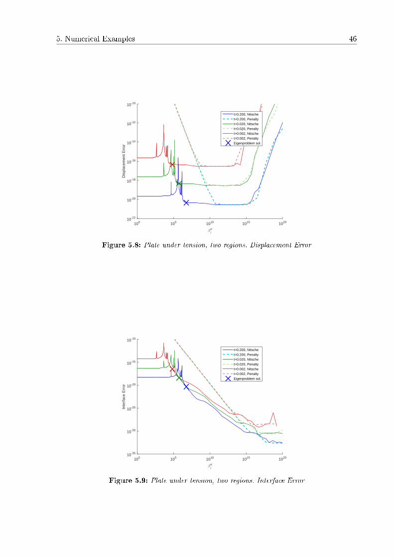
5. Numerical Examples 46
βu
i
100 105 1010 1015 1020
Dis
plac
emen
t Err
or
10-22
10-20
10-18
10-16
10-14
10-12
10-10
t=0.200, Nitschet=0.200, Penaltyt=0.020, Nitschet=0.020, Penaltyt=0.002, Nitschet=0.002, PenaltyEigenproblem sol.
Figure 5.8: Plate under tension, two regions. Displacement Error
βu
i
100 105 1010 1015 1020
Inte
rfac
e E
rror
10-35
10-30
10-25
10-20
10-15
10-10
t=0.200, Nitschet=0.200, Penaltyt=0.020, Nitschet=0.020, Penaltyt=0.002, Nitschet=0.002, PenaltyEigenproblem sol.
Figure 5.9: Plate under tension, two regions. Interface Error

5. Numerical Examples 47
-0.5 0 0.5 1 1.5 2 2.5
0
0.5
1
1.5
2
Gu
rGi
r
Gt
r
er
1
er
2
er
3
Figure 5.10: Plate under pure bending, two regions.
βu
i
100 105 1010 1015
Dis
plac
emen
t Err
or
10-20
10-15
10-10
10-5
100
105
1010
t=0.200, Nitschet=0.200, Penaltyt=0.020, Nitschet=0.020, Penaltyt=0.002, Nitschet=0.002, PenaltyEigenproblem sol.
Figure 5.11: Plate under pure bending, two regions. Displacement Error
on the interface. Once again, the maximum eigenvalue of the proposed system correctly
approximates the end of the unstable zone and the baselines of the error curves are wide
enough to accommodate values of 1 ≤ α ≤ 1×10⁷ approximately.
5.2.2 Rotation DOFs
For the particle distribution in Fig. 5.10, several values of βθi where used as to assess
the error in the interface continuity. The values of βuu and βθu were taken according to
(4.80) with α = 10 and for βui , α = 1.
The results are presented in Figs. 5.11, 5.12 and similar conclusions can be drawn. The
solution of the proposed eigenproblem is clear of the perturbed region by a considerable
margin, still away of the numerical instabilities of a pure penalty approach.

5. Numerical Examples 48
βu
i
100 105 1010 1015
Inte
rfac
e E
rror
10-20
10-15
10-10
10-5
100
105
t=0.200, Nitschet=0.200, Penaltyt=0.020, Nitschet=0.020, Penaltyt=0.002, Nitschet=0.002, PenaltyEigenproblem sol.
Figure 5.12: Plate under pure bending, single region. Essential Boundary Error
0
0.5
11
0.5
0
0.8
0
0.2
0.4
0.6
er
1
er
2
er
3
1 0.
0
0.5
11
0.5
0
0.8
0
0.2
0.4
0.6
er
1
er
2
er
3
1 0.
0
0.5
11
0.5
0
0.8
0
0.2
0.4
0.6
er
1
er
2
er
3
1 0.
(a) (b) (c)
0
0.5
11
0.5
0
0.8
0
0.2
0.4
0.6
er
1
er
2
er
3
1 0.
0
0.5
11
0.5
0
0.8
0
0.2
0.4
0.6
er
1
er
2
er
3
1 0.
(d) (e)
Figure 5.13: Pinched Cylinder. Discretization models A, B and C respectively

5. Numerical Examples 49
5.3 Pinched Cylinder
The classical Pinched Cylinder [56] example is presented next. It consists of a cylindri-
cal shell with rigid diaphragms on each end subject to two opposing concentrated loads
pinching its center point inwards. For simplicity, we model only one eighth of the cylinder,
depicted in Fig. 5.13. The shell has a thickness of 0.01, Young modulus of 98 and Poisson
ratio of 0.3. The length of the full cylinder is 2.0 and its radius 1.0. The applied load is
1/1200 downwards.
The MLS shape functions were constructed using a fth order polynomial base and a
support radius amplied by 3. The use of a high-order base is demanding on the particle
distribution concerning linear dependencies. The particles are then moved from a straight
structured distribution by a small random perturbation. Particles may lay outside the
approximation domain, as long as their support covers at least part of it. In this case, the
particles don't coincide with the nodes of the integration cell discretization depicted in
Fig. 5.13.
Five dierent models were developed and compared. Model A uses a single region with
almost uniform particle distribution and no interface. Model B divides the domain into
two regions through a interface at ξ1 = 0.5 with both regions approximated by similar
particle distributions. It serves to demonstrate that the present framework can reproduce
curved interfaces. Model C, also uses two discretization regions, but with the blue region
more rened than the yellow region. This illustrates the possibility of local renement,
equivalent to non conforming FE meshes. Models D and E have similar denitions as B
and C, but with a longitudinal interface. Particle distributions for models A, B, C, D and
E are all depicted in Fig. 5.13.
Kinematic constraints are enforced either with Lagrange Multipliers or with Nitsche's
Method using the eigenvalue problem solution and all α = 10. For the Lagrange Mul-
tipliers, the linear solver warned for badly scaled system matrix if the trivial choice of
discretization was chosen for the interface and the essential boundary. As results were
similar to the ones obtained with Nitsche's method for similar particle distributions, we
trust that the MATLAB solver could handle the badly scaled system.
Fig. 5.14 shows the vertical displacement of the loaded point. Results converge to
the reference solution −6.0829 × 10⁻⁸, with the same ratio for Nitsche's method as for
Lagrange multipliers.
It is noticeable that Model B converges with similar ratio as Model A, but requires
more DOFs to achieve the same error. This is expected as the use of two regions with same
approximation properties brings no signicant advantage in this case. The approximation
space is not enriched in this area.
As for Model C, convergence is kept at a similar ratio, but again we need too many
DOFs to achieve the same level of error. Even thought Nitsche's Method precludes the

5. Numerical Examples 50
0 500 1000 1500 2000 2500 3000 3500 4000 4500 5000
× 10-8
1
2
3
4
5
6
Model A Lag
Model A Nit
Model B Lag
Model B Nit
Model C Lag
Model C Nit
Model D Lag
Model D Nit
Model E Lag
Model E Nit
Figure 5.14: Pinched Cylinder. Loaded point displacements

5. Numerical Examples 51
Figure 5.15: Pinched Cylinder. Deformed shape
introduction of interface DOFs, the separate approximations requires the nodes on the
interface to be doubled. These extra DOFs are also present in the Lagrange Multiplier
framework as it relates to the discretization rather then to the kinematic constraint.
Models D and E, with a shorter interface, don't need so many DOFs introduced. Model
E presents the best results for a same number of DOFs as renement is carried out in
the area with higher gradients. A representation of the displacements on the converged
solution is depicted in Fig. 5.15
5.4 T-beam
A balance T-beam under concentrated load is analyzed in [22] and reproduced in
Fig. 5.16. Young modulus was taken as 3×10⁶ and Poisson's ratio 0.3. This example
presents a possibility to analyze a structure assembled from shells in dierent planes. The
interface is the line on the intersection of the shells' midsurfaces.
The solution present in [22] and depicted in Fig. 5.16(a) includes a interface inside
the domain. Despite departing from the described framework, it presents no dierence in
implementation and forms our 2-region model. Nevertheless, for the balance of moments
on the intersection between the ange and the web to be kept, the moment acting on the
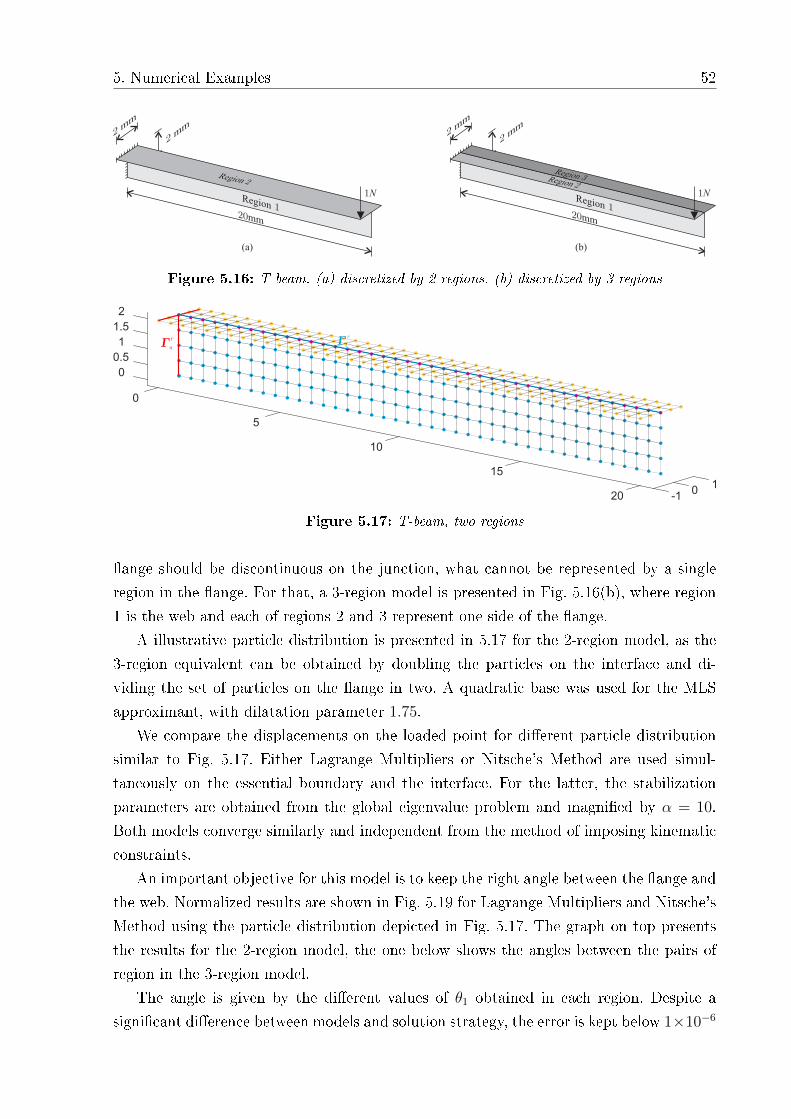
5. Numerical Examples 52
20mm
Region 1
2m
m
2m
m
1N
Region 2
20mm
Region 1
2m
m
2m
m
1N
Region 2
Region 3
(a) (b)
Figure 5.16: T-beam. (a) discretized by 2 regions. (b) discretized by 3 regions
5
0
2
1
0.5
0
1.5
10
20
15
-1
10
Gu
r Gi
r
Figure 5.17: T-beam, two regions
ange should be discontinuous on the junction, what cannot be represented by a single
region in the ange. For that, a 3-region model is presented in Fig. 5.16(b), where region
1 is the web and each of regions 2 and 3 represent one side of the ange.
A illustrative particle distribution is presented in 5.17 for the 2-region model, as the
3-region equivalent can be obtained by doubling the particles on the interface and di-
viding the set of particles on the ange in two. A quadratic base was used for the MLS
approximant, with dilatation parameter 1.75.
We compare the displacements on the loaded point for dierent particle distribution
similar to Fig. 5.17. Either Lagrange Multipliers or Nitsche's Method are used simul-
taneously on the essential boundary and the interface. For the latter, the stabilization
parameters are obtained from the global eigenvalue problem and magnied by α = 10.
Both models converge similarly and independent from the method of imposing kinematic
constraints.
An important objective for this model is to keep the right angle between the ange and
the web. Normalized results are shown in Fig. 5.19 for Lagrange Multipliers and Nitsche's
Method using the particle distribution depicted in Fig. 5.17. The graph on top presents
the results for the 2-region model, the one below shows the angles between the pairs of
region in the 3-region model.
The angle is given by the dierent values of θ1 obtained in each region. Despite a
signicant dierence between models and solution strategy, the error is kept below 1×10⁻⁶

5. Numerical Examples 53
DOFs ×104
0 0.5 1 1.5 2 2.5 3 3.5 4
Tip
Dis
plac
emen
t
×10-3
4.1
4.15
4.2
4.25
4.3
4.35
4.4
4.45
Lag Mult 2-regionsNitsches 2-regionsLag Mult 3-regionsNitsches 3-regions
Figure 5.18: T-beam, tip displacement
angle
/ (
pi/2)
× 10 -7
-2
0
2
4
6
8
10
12Angle between regions
Solution with 2 regions
Solution with 3 regions
Lag Mult
Nitsches
Interface length
0 5 10 15 20
angle
/ (
pi/2)
-2
0
2
4
6
8
10
Lag Mult r1-r2
Lag Mult r1-r3
Nitsches r1-r2
Nitsches r1-r3
Figure 5.19: T-beam, angle between regions

5. Numerical Examples 54
Figure 5.20: T-beam, moments for 2-region model
for the worst situation.
The 2-region model emulates the overall behavior really well, with compatible results
for tip displacement, however cannot represent a sharp stress jump. Figs. 5.20-5.21 show
a top view of the twisting moment m21 for each approach and exemplies how a 3-region
model can be useful. Fig. 5.22 shows the deformed model with amplied displacements

5. Numerical Examples 55
Figure 5.21: T-beam, moments for 3-region model
Figure 5.22: T-beam, displacements for 3-region model

Chapter 6
Conclusions
This work has presented an alternative for imposing kinematic conditions in the linear
analysis of shear deformable shells using the Element-Free Galerkin method: Nitsche's
method. The approach is adapted to the shear deformable shell model and suitable for
Element-free Galerkin analysis, accounting for rotation degrees of freedom and bending
tractions. It is compared to more usual Penalty and Lagrange Multiplier methods, and
consistency between weak and strong formulation is demonstrated. Numerical simulations
present similar rates of convergence for the three methods, with no addition of degrees of
freedom or loss of consistency for a wider range of stabilization parameters for Nitsche's
approach.
One of the setbacks of Nitsche's Method is the presence of a user dened stabilization
penalty-like parameter. The choice is not as fundamental as in a pure penalty parameter as
the range of suitable values is wider. Nevertheless, the use of rotational degrees of freedom
and bending stiness, which assume dierent order of magnitude than the displacement
DOFs and dierent dependency on the shell thickness, narrows the decision space if the
parameter were to be taken as the same for all elds. We overcome this barrier proposing
dierent parameters β for each set of DOFs and proposing eigenvalue problems to estimate
a lower bound. The matrices used for the eigenvalue problem are either already computed
during domain assembly or have components already calculated for boundary imposition.
Even more, only the higher eigenvalue is needed, so the assembly and solution of the
eigenvalue problem is not so demanding during computation.
Even so, some measures could be implemented as to speed the process. If the approx-
imations are similar (same material properties and similar particle spacing), the result
obtained for one boundary can be used on the others and the interfaces. A local approach
for the eigenvalue problem is available for Finite Elements [15], where the mesh dependent
inequalities are expressed in a single element's domain thus assembling and solving the
eigenproblem with only one element's degrees of freedom. The stabilization parameter
is then taken as the largest of the element-wise estimations or as variable on the inter-
face. The lack of elements makes the extension to meshless methods not straightforward,
56

6. Conclusions 57
but possible via boundary integration cells. These alternatives are left as possibilities for
future research. Extension to nonlinear problems is another desired feature, as it would
emphasize the advantage of a smaller system of equations.
Numerical results show that the method is ecient, with similar error and convergence
properties as Lagrange Multipliers and more stable than the Penalty method. Flexibil-
ity was demonstrated as curved interfaces, folded shells and discretization with dierent
particle density were accurately represented.
The developed model proves suitable for shell analysis under small displacement and
rotations, keeping a neat formulation whose weak form correspond to the dierential
statements with no need for a secondary approximation eld or a hybrid formulation.
The extension of Nitsche's weak for to encompass rotational DOFs was successful and the
estimation procedure for stabilization parameters renders a proper lower bound and thus
a stable formulation.
These contributions were summarized and submitted for publication by Costa, Pi-
menta and Wriggers [11].

Bibliography
[1] C. Annavarapu, M. Hautefeuille, and J. E. Dolbow. A robust Nitsche's formulation
for interface problems. Computer Methods in Applied Mechanics and Engineering,
225-228(0):44 54, 2012. 2, 32, 36
[2] C. Annavarapu, M. Hautefeuille, and J. E. Dolbow. Stable imposition of sti con-
straints in explicit dynamics for embedded nite element methods. International
Journal for Numerical Methods in Engineering, 92(2):206 228, 2012. 2
[3] C. Annavarapu, M. Hautefeuille, and J. E. Dolbow. A nitsche stabilized nite element
method for frictional sliding on embedded interfaces. part ii: Intersecting interfaces.
Computer Methods in Applied Mechanics and Engineering, 267:318 341, 2013. 2
[4] C. Annavarapu, M. Hautefeuille, and J. E. Dolbow. A Nitsche stabilized nite ele-
ment method for frictional sliding on embedded interfaces. Part I: Single interface.
Computer Methods in Applied Mechanics and Engineering, 268:417 436, 2014. 2
[5] T. Belytschko, Y. Krongauz, D. Organ, M. Fleming, and P. Krysl. Meshless methods:
An overview and recent developments. Computer Methods in Applied Mechanics and
Engineering, 139(1-4):3 47, 1996. 21
[6] T. Belytschko, Y. Y. Lu, and L. Gu. Element-free galerkin methods. International
Journal for Numerical Methods in Engineering, 37(2):229256, 1994. 1, 16, 20, 22
[7] T. Belytschko, D. Organ, and Y. Krongauz. A coupled nite element-element-free
galerkin method. Computational Mechanics, 17(3):186195, 1995. 2, 20
[8] F. Cirak, M. Ortiz, and P. Schröder. Subdivision surfaces: a new paradigm for
thin-shell nite-element analysis. International Journal for Numerical Methods in
Engineering, 47(12):20392072, 2000. 10
[9] L. W. Cordes and B. Moran. Treatment of material discontinuity in the element-
free galerkin method. Computer Methods in Applied Mechanics and Engineering,
139(1-4):75 89, 1996. 2, 21
[10] J. C. Costa. Análise linear de cascas com método de galerkin livre de elementos.
Master's thesis, Polytechnical School at the University of Sao Paulo, 2010. 4
58

BIBLIOGRAPHY 59
[11] J. C. Costa, P. de Mattos Pimenta, and P. Wriggers. Meshless analysis of shear
deformable shells: boundary and interface constraints. Computational Mechanics,
recently submitted. 57
[12] J. C. Costa, C. M. Tiago, and P. de Mattos Pimenta. Meshless analysis of shear
deformable shells: the linear model. Computational Mechanics, 52(4):763 778, 2013.
1, 2, 4, 10, 12, 18
[13] E. M. de Barreto Campello, P. de Mattos Pimenta, and P. Wriggers. A triangu-
lar nite shell element based on a fully nonlinear shell formulation. Computational
Mechanics, 31(6):505518, 2003. 11
[14] P. de Mattos Pimenta and E. M. de Barreto Campello. Shell curvature as an initial
deformation: A geometrically exact nite element approach. International Journal
for Numerical Methods in Engineering, 78(9):10941112, 2009. 2, 4
[15] J. Dolbow and I. Harari. An ecient nite element method for embedded interface
problems. International Journal for Numerical Methods in Engineering, 78(2):229
252, 2009. 2, 21, 36, 56
[16] A. Embar, J. Dolbow, and I. Harari. Imposing dirichlet boundary conditions with
nitsche's method and spline-based nite elements. International Journal for Numer-
ical Methods in Engineering, 83(7):877 898, 2010. 2, 36
[17] S. Fernández-Méndez, J. Bonet, and A. Huerta. Continuous blending of SPH with
nite elements. Computers & Structures, 83(17-18):1448 1458, 2005. Advances in
Meshfree Methods. 20
[18] S. Fernández-Méndez and A. Huerta. Imposing essential boundary conditions in
mesh-free methods. Computer Methods in Applied Mechanics and Engineering,
193(12-14):1257 1275, 2004. Meshfree Methods: Recent Advances and New Ap-
plications. 1, 2, 20, 31, 36
[19] A. Fritz, S. Hüeber, and B. I. Wohlmuth. A comparison of mortar and nitsche
techniques for linear elasticity. CALCOLO, 41(3):115137, 2004. 21
[20] M. Griebel and M. A. Schweitzer. A particle-partition of unity method Part V:
Boundary conditions. InGeometric Analysis and Nonlinear Partial Dierential Equa-
tions. 2, 36
[21] Y. Guo and M. Ruess. A layerwise isogeometric approach for NURBS-derived lami-
nate composite shells. Composite Structures, 124:300 309, June 2015. 22

BIBLIOGRAPHY 60
[22] Y. Guo and M. Ruess. Nitsche's method for a coupling of isogeometric thin shells and
blended shell structures. Computer Methods in Applied Mechanics and Engineering,
284:881 905, Feb. 2015. 2, 22, 51
[23] Y. Guo and M. Ruess. Weak Dirichlet boundary conditions for trimmed thin isoge-
ometric shells. Computers & Mathematics with Applications, June 2015. 2, 22
[24] A. Hansbo and P. Hansbo. An untted nite element method, based on nitsche's
method, for elliptic interface problems. Computer Methods in Applied Mechanics and
Engineering, 191(4748):55375552, 2002. 21
[25] I. Harari and J. E. Dolbow. Analysis of an ecient nite element method for em-
bedded interface problems. Computational Mechanics, 46(1):205 211, 2010. 2
[26] I. Harari and E. Grosu. A unied approach for embedded boundary conditions
for fourth-order elliptic problems. International Journal for Numerical Methods in
Engineering, pages n/an/a, 2014. 2
[27] I. Harari and E. Shavelzon. Embedded kinematic boundary conditions for thin plate
bending by nitsche's approach. International Journal for Numerical Methods in En-
gineering, 92(1):99 114, 2012. 2, 38
[28] M. Hautefeuille, C. Annavarapu, and J. E. Dolbow. Robust imposition of dirichlet
boundary conditions on embedded surfaces. International Journal for Numerical
Methods in Engineering, 90(1):40 64, 2012. 2, 21
[29] A. Huerta and S. Fernández-Méndez. Enrichment and coupling of the nite element
and meshless methods. International Journal for Numerical Methods in Engineering,
48(11):16151636, 2000. 2, 20
[30] A. Huerta, S. Fernández-Méndez, and W. K. Liu. A comparison of two formulations
to blend nite elements and mesh-free methods. Computer Methods in Applied Me-
chanics and Engineering, 193(12-14):1105 1117, 2004. Meshfree Methods: Recent
Advances and New Applications. 20
[31] V. Ivannikov, C. Tiago, and P. M. Pimenta. Meshless implementation of the geomet-
rically exact kirchho-love shell theory. International Journal for Numerical Methods
in Engineering, 100(1):1 39, 2014. 1, 2
[32] V. Ivannikov, C. Tiago, and P. M. Pimenta. On the boundary conditions of the
geometrically nonlinear kirchho-love shell theory. International Journal of Solids
and Structures, 51(18):3101 3112, 2014. 2

BIBLIOGRAPHY 61
[33] W. Jiang, C. Annavarapu, J. E. Dolbow, and I. Harari. A robust nitsche's formulation
for interface problems with spline-based nite elements. International Journal for
Numerical Methods in Engineering, 2015. 2
[34] L. A. B. Jr., O. L. Manzoli, P. G. Prazeres, E. A. Rodrigues, and T. N. Bittencourt.
A coupling technique for non-matching nite element meshes. Computer Methods in
Applied Mechanics and Engineering, 290:19 44, 2015. 21
[35] Y. Krongauz and T. Belytschko. Enforcement of essential boundary conditions in
meshless approximations using nite elements. Computer Methods in Applied Me-
chanics and Engineering, 131(1-2):133 145, 1996. 1, 20
[36] Y. Krongauz and T. Belytschko. Efg approximation with discontinuous derivatives.
International Journal for Numerical Methods in Engineering, 41(7):1215 1233, 1998.
21
[37] P. Krysl and T. Belytschko. Analysis of thin shells by the element-free galerkin
method. International Journal of Solids and Structures, 33(20-22):3057 3080, 1996.
1
[38] S. Li, W. Hao, and W. K. Liu. Numerical simulations of large deformation of thin
shell structures using meshfree methods. Computational Mechanics, 25(2-3):102116,
2000. 1
[39] S. Li and W. K. Liu. Meshfree Particle Methods. Springer, Berlin, 2004. 2, 16
[40] G. R. Liu. Mesh Free methods: Moving beyond the nite element method. CRC Press,
2010. 16
[41] G. R. Liu and Y. T. Gu. An Introduction to Meshfree Methods and Their Program-
ming. Springer Netherlands, Dordrecht, 2005. 18, 20
[42] Y. Lu, T. Belytschko, and L. Gu. A new implementation of the element free galerkin
method. Computer Methods in Applied Mechanics and Engineering, 113(3-4):397
414, 1994. 2, 20, 33
[43] Y. Lu, T. Belytschko, and M. Tabbara. Element-free galerkin method for wave
propagation and dynamic fracture. Computer Methods in Applied Mechanics and
Engineering, 126(1-2):131 153, 1995. 2, 20
[44] MATLAB. version 8.5.0 (R2015a). The MathWorks Inc., Natick, Massachusetts,
2015. 24

BIBLIOGRAPHY 62
[45] B. Nayroles, G. Touzot, and P. Villon. Generalizing the nite element method: Diuse
approximation and diuse elements. Computational Mechanics, 10(5):307318, 1992.
16, 22
[46] V. P. Nguyen, P. Kerfriden, M. Brino, S. P. A. Bordas, and E. Bonisoli. Nitsches
method for two and three dimensional nurbs patch coupling. Computational Mechan-
ics, 53(6):1163 1182, 2014. 2, 31, 36
[47] J. Nitsche. Über ein variationsprinzip zur lösung von dirichlet-problemen bei verwen-
dung von teilräumen, die keinen randbedingungen unterworfen sind. Abhandlungen
aus dem Mathematischen Seminar der Universität Hamburg, 36(1):915, 1971. 2, 20,
31
[48] H. Noguchi, T. Kawashima, and T. Miyamura. Element free analyses of shell and
spatial structures. International Journal for Numerical Methods in Engineering,
47(6):12151240, 2000. 1
[49] M. Ruess, D. Schillinger, Y. Bazilevs, V. Varduhn, and E. Rank. Weakly enforced es-
sential boundary conditions for NURBS-embedded and trimmed NURBS geometries
on the basis of the nite cell method. International Journal for Numerical Methods
in Engineering, 95(10):811 846, Sept. 2013. 2, 21, 33, 36
[50] M. Ruess, D. Schillinger, A. I. Özcan, and E. Rank. Weak coupling for isogeometric
analysis of non-matching and trimmed multi-patch geometries. Computer Methods
in Applied Mechanics and Engineering, 269:4671, Feb. 2014. 2, 21, 36
[51] E. Sala-Lardies, S. Fernández-Méndez, and A. Huerta. Optimally convergent high-
order x-fem for problems with voids and inclusions. pages 80808093, 2012. 2
[52] J. D. Sanders, J. E. Dolbow, and T. A. Laursen. On methods for stabilizing con-
straints over enriched interfaces in elasticity. International Journal for Numerical
Methods in Engineering, 78(9):1009 1036, 2009. 2, 36, 38
[53] J. D. Sanders, T. A. Laursen, and M. A. Puso. A nitsche embedded mesh method.
Computational Mechanics, 49(2):243 257, 2012. 2, 21, 32, 36
[54] J. D. Sanders and M. A. Puso. An embedded mesh method for treating overlapping
nite element meshes. International Journal for Numerical Methods in Engineering,
91(3):289 305, 2012. 2
[55] J. Simo and T. Hughes. Computational Inelasticity. Interdisciplinary applied math-
ematics: Mechanics and materials. Springer, 1998. 11

BIBLIOGRAPHY 63
[56] J. C. Simo, D. D. Fox, and M. S. Rifai. On a stress resultant geometrically exact
shell model. part ii: The linear theory; computational aspects. Computer Methods in
Applied Mechanics and Engineering, 73(1):53 92, 1989. 49
[57] R. Stenberg. On some techniques for approximating boundary conditions in the nite
element method. Journal of Computational and Applied Mathematics, 63(1-3):139
148, 1995. Proceedings of the International Symposium on Mathematical Modelling
and Computational Methods Modelling 94. 2
[58] C. M. Tiago. Meshless methods: Extending the linear formulation and its gener-
alization to geometrically exact structural analysis. PhD thesis, Instituto Superior
Técnico, Universidade Técnica de Lisboa, 2007. 1, 2, 16, 18, 33
[59] P. Wriggers and G. Zavarise. A formulation for frictionless contact problems using a
weak form introduced by nitsche. Computational Mechanics, 41(3):407420, 2008. 2
[60] T. Zhu and S. N. Atluri. A modied collocation method and a penalty formulation
for enforcing the essential boundary conditions in the element free galerkin method.
Computational Mechanics, 21(3):211222, 1998. 27