STABILITY RADII FOR LINEAR HAMILTONIAN SYSTEMS WITHDISSIPATION UNDER STRUCTURE-PRESERVING PERTURBATIONS

CHRISTIAN MEHL∗, VOLKER MEHRMANN∗, AND PUNIT SHARMA∗

Abstract. Dissipative Hamiltonian (DH) systems are an important concept in energy based modeling ofdynamical systems. One of the major advantages of the DH formulation is that system properties are encoded inan algebraic way. For instance, the algebraic structure of DH systems guarantees that the system is automaticallystable. In this paper the question is discussed when a linear constant coefficient DH system is on the boundary ofthe region of asymptotic stability, i.e., when it has purely imaginary eigenvalues, or how much it has to be perturbedto be on this boundary. For unstructured systems this distance to instability (stability radius) is well-understood.In this paper, explicit formulas for this distance under structure-preserving perturbations are determined. It is alsoshown (via numerical examples) that under structure-preserving perturbations the asymptotical stability of a DHsystem is much more robust than under general perturbations, since the distance to instability can be much largerwhen structure-preserving perturbations are considered.

Keywords dissipative Hamiltonian system, port-Hamiltonian system, distance to instability,structure-preserving distance to instability, restricted distance to instabilityAMS subject classification. 93D20, 93D09, 65F15, 15A21, 65L80, 65L05, 34A30.

1. Introduction. In recent years energy based modeling approaches have gained great at-tention. When a model arises from variational principles, then it is often characterized by aport-Hamiltonian (PH) system, see [5, 9, 26, 28, 29, 32, 31, 34, 35, 36] for some major references.

Linear constant coefficient input-state-output PH systems have the form

x = (J −R)Qx+ (B − P )u, (1.1)

y = (B + P )HQx+ (S +N)u,

where x is the state, u the input, and y the output. The Hamiltonian, i.e., the function x 7→ xHQxwith Q = QH ∈ Cn,n being positive definite, describes the energy of the system; J = −JH ∈ Cn,nis the structure matrix describing the energy flux among energy storage elements within thesystem; R = RH ∈ Cn,n is the dissipation matrix describing energy dissipation/loss in the system;B ± P ∈ Cn,m are the port matrices, describing the manner in which energy enters and exits thesystem, and the matrix S + N , with S = SH ∈ Cm,m and N = −NH ∈ Cm,m, describes directfeed-through from input to output. In a PH system the matrices R, P , and S must satisfy

K =

[R P

PH S

]≥ 0; (1.2)

i.e., K is symmetric positive semidefinite. In particular, R must also be positive semidefinite.PH systems have many important geometric and algebraic properties that are nicely encoded

in the way the system is represented, see [5, 18, 29]. In this paper, we focus on the property thatPH systems are stable, i.e., all eigenvalues of the system matrix A = (J − R)Q are contained inthe closed left half complex plane and all eigenvalues on the imaginary axis are semisimple. Tostudy stability, the port matrices can be ignored, and so one is left with a dissipative Hamiltonian(DH) system of the form

x = (J −R)Qx. (1.3)

The stability of the system is then due to the fact that Q is Hermitian positive definite. Indeed,for any nonzero vector z one has

Re(zH(Q1/2AQ−1/2)z

)= Re

(zH(Q1/2JQ1/2 −Q1/2RQ1/2)z

)= −zHQ1/2RQ1/2z ≤ 0

∗Institut fur Mathematik, MA 4-5, TU Berlin, Straße des 17. Juni 136, D-10623 Berlin, Germany. Email:mehl,mehrmann,sharma@math.tu-berlin.de.

Supported by Einstein Stiftung Berlin through the Research Center Matheon Mathematics for key technolo-gies in Berlin and by ERC advanced grant MODSIMCONMP.

1

since R is positive semidefinite. (Concerning semisimplicity of the eigenvalues on the imaginaryaxis, we refer to Lemma 3.1.)

If one would multiply out the product to form the matrix A and forget about the DH-structureof the system, then stability would not be obvious anymore. To check whether the system is stable,one can compute the eigenvalues or use Lyapunov’s theorem [21]. If A has purely imaginary eigen-values then arbitrarily small perturbations (such as data or roundoff errors) may move eigenvaluesinto the right half plane. This is particularly the case for linear systems which arise as linearizationof nonlinear systems around stationary reference solutions [4], from data driven realizations, see,e.g., [1, 27], or from classical finite element modeling [11]. In all these and many other cases thesystem model is subject to perturbations and the stability of the systems can only be guaranteedwhen the system has a reasonable distance to instability, see [14, 16]. Computing the distance toinstability [3, 7, 13, 40] is an optimization problem and again subject to perturbations.

The situation is different for DH systems which are automatically stable, whatever the pertur-bations are, as long as they preserve the DH structure. However, DH systems are not necessarilyasymptotically stable, i.e., they may have purely imaginary eigenvalues. So for a DH system it isimportant to know whether the system is just stable or even asymptotically stable, and even morewhether it is robustly asymptotically stable, i.e., small (structured) perturbations keep it asymptot-ically stable. The latter requires that the system has a reasonable distance to a DH system withpurely imaginary eigenvalues. To study this question is an important topic in many applications,in particular, in power system and circuit simulation, see, e.g. [24, 25, 23, 30], and multi-bodysystems, see, e.g. [11, 37, 41].

Example 1.1. In the finite element analysis of disk brake squeal [11], large scale second orderdifferential equations arise that have the form

Mq + (D +G)q + (K +N)q = f,

where M = MH > 0 is the mass matrix, D = DH ≥ 0 models material and friction induceddamping, G = −GH models gyroscopic effects, K = KH > 0 models the stiffness and N , isa nonsymmetric matrix modeling circulatory effects. An appropriate first order formulation isassociated with the linear pencil λI + (J −R)Q, where

J :=

[G K + 1

2N−(K + 1

2NH) 0

], R :=

[D 1

2N12N

H 0

], Q :=

[M 00 K

]−1

, (1.4)

where I denotes the identity matrix.

Break squeal is associated with eigenvalues in the right half plane. If the matrix N vanishes,then the system is automatically stable, since it is a DH system. One can view the matrix N as a(small-rank) perturbation of a DH system since in the industrial examples considered in [11], thematrix N has a rank of order 2000 and the size of the system is of order 1 million. It is obviousthat for N 6= 0 the pencil λI+ (J −R)Q is missing one of the essential properties of a DH system,because the matrix R is then indefinite and thus the system may be unstable which is the reasonfor squeal. To analyze properties of the system (1.1) when this happens is one of the motivationsfor our work.

Example 1.2. A different and more general class of DH descriptor systems of the form

Mx = (J −R)Qx (1.5)

arises in circuit simulation as well as power system modeling. Consider e.g. a simple example ofan RLC network, see [8], given by a differential-algebraic equation GcCGTc 0 0

0 L 00 0 0

︸ ︷︷ ︸

:=M

v(t)

il(t)

iv(t)

=

−GrR−1GTr −Gl −GvGTl 0 0GTv 0 0

︸ ︷︷ ︸

:=J−R

v(t)il(t)iv(t)

, (1.6)

2

with real symmetric matrices L > 0, C > 0, R > 0 incorporating the resistances of the resistors,capacitances of the capacitors, and inductances between the inductors, respectively.

Here, (J − R) is the graph incidence matrix, Gv is of full rank, and the subscripts r, c, l, vand i refer to edge quantities corresponding to the resistors, capacitors, inductors, voltage sourcesand current sources, respectively, of the given RLC network. In this case we have

J =

0 −Gl −GvGTl 0 0GTv 0 0

, R =

GrR−1GTr 0 00 0 00 0 0

, Q := I.

Since M is singular, this system has algebraic constraints (arising from Kirchhoff’s laws), i.e.,eigenvalues at ∞ and since Gv has full row rank, it is is of index two, i.e., the system has Jordanblocks at ∞ of size two, [6]. Applying an index reduction procedure [20, 33] and solving thealgebraic constraint equations (which one would not do in practice) leads to a DH system for thedynamic variables

M z = (J − R)z, (1.7)

where M is invertible. Setting Q = M−1 and x = Mz then gives a DH system as in (1.3).In this paper, we focus on perturbations of DH systems that affect only one of the coefficient

matrices R, J , or Q. We also allow perturbations of the form B∆C, where B ∈ Cn,r and C ∈ C`,nare of full column rank or full row rank, respectively. This allows the consideration of perturbationsthat only affect restricted parts of matrices. For example, if

D ∈ Cr,r, R =

[D 00 0

]∈ Cn,n, B = CH =

[Ir0

]∈ Cn,r,

then perturbations of the form B∆C will only affect the block D, but will leave the zero blocks inR unchanged. While perturbations of the form B∆C were called structured perturbations in [15],we will call them restricted perturbations instead, because “structured” could be misinterpreted asreferring to the additional port-Hamiltonian structure of the system.

The paper is organized as follows. In Section 2 we study some mapping theorems that willbe needed to characterize the stability distances under consideration. In Section 3 we define thevarious stability distances that we will discuss in this paper and give explicit formulas when onlyone of the matrices R, J , or Q is perturbed and structure is ignored. Then we develop explicitformulas or bounds for stability distances while focussing on structure-preserving perturbationsthat individually perturb only R, J , or Q in Sections 4, 5, and 6, respectively. In Section 7we provide some numerical experiments to illustrate our results and, in particular, to show thatthe stability distances under structure-reserving perturbations may differ significantly from thecorresponding ones under general perturbations.

In the following ‖ · ‖ denotes the spectral norm of a vector or a matrix while ‖ · ‖F denotesthe Frobenius norm of a matrix. By Λ(A) we denote the spectrum of a matrix A ∈ Cn,n, whereCn,r is the set of complex n × r matrices, with the special case Cn = Cn,1. The sets Herm(n)and SHerm(n), respectively, denote the set of complex Hermitian and skew-Hermitian matricesin Cn,n. We use the notation A ≥ 0 and A ≤ 0 if A ∈ Cn,n is positive or negative semidefinite,respectively, and A > 0 if A is positive definite.

For a matrix A ∈ Cn,r we denote by A† ∈ Cr,n the Moore-Penrose inverse of A, see e.g., [10].We denote the identity matrix of size n by In. Finally, σmin(A) denotes the smallest singular valueof A, and if A is Hermitian, then λmax(A) and λmin(A) denote its largest or smallest eigenvalue,respectively.

2. Mapping theorems. An important tool in the theory of distance problems are so-calledstructured mapping problems, i.e., finding necessary and sufficient conditions on vectors x, y ∈ Cnfor the existence of matrices ∆ with a given symmetry structure that map x to y, and characterizingall such matrices that are of minimal norm. In this section we discuss some mapping results thatwill be necessary to compute the stability distances.

3

The minimal norm solutions for the Hermitian mapping problem with respect to both thespectral norm and the Frobenius norm are well known, see [22]. In order to allow a direct applica-tion in later sections of this paper, we restate the result concerning the spectral norm in the formgiven in [2] which is a slightly different form than the one in [22].

Theorem 2.1. Let x, y ∈ Cn \ 0. Then there exists a matrix H ∈ Herm(n) such thatHx = y if and only if xHy ∈ R. If the latter condition is satisfied then we have

min‖H‖

∣∣ H ∈ Cn,n, HH = H, Hx = y

=‖y‖‖x‖

and the minimum is attained for the matrix

H :=‖y‖‖x‖

[y‖y‖

x‖x‖

] [ yHx‖x‖ ‖y‖ 1

1 xHy‖x‖ ‖y‖

]−1 [y‖y‖

x‖x‖

]H(2.1)

if x and y are linearly independent and for H := yxH

xHxotherwise.

As the minimal norm matrices presented in Theorem 2.1 typically have rank 2 unless x andy are linearly dependent, one may ask whether there exists also matrices solving the Hermitianmapping problem that have rank one, and indeed it is well known that such matrices exists, see,e.g., [22, Theorem 5.1]. Interestingly, as we will show below, these matrices are not only minimalin rank, but they are also minimal norm solutions to the slightly different mapping problem, wherethe matrices are not only required to be Hermitian, but also to be semidefinite. For the proofof the following theorem, where we will characterize all Hermitian semidefinite solutions to ourmapping problem, we will need the following lemma.

Lemma 2.2 ([38, Lemma 1.3]). Let A ∈ Cp,m, B ∈ Cn,q, C ∈ Cp,q, and

Υ =E ∈ Cm,n

∣∣AEB = C.

Then Υ 6= ∅ if and only if A,B,C satisfy AA†CB†B = C. If the latter condition is satisfied then

Υ =A†CB† + Z −A†AZBB†

∣∣Z ∈ Cn,n.

Using this Lemma, we have the following mapping theorem with Hermitian positive semidefinitesolutions.

Theorem 2.3. Let x, y ∈ Cn \ 0 and let

S :=H ∈ Cn,n

∣∣HH = H, H ≥ 0, Hx = y. (2.2)

Then there exists a positive semidefinite Hermitian matrix H ∈ Herm(n) such that Hx = y (i.e.,we have S 6= ∅) if and only if xHy > 0. If the latter condition is satisfied then

min‖H‖

∣∣ H ∈ S =‖y‖2

xHy(2.3)

and the minimum is attained for the rank one matrix

H =1

xHyyyH . (2.4)

Furthermore, we have

S =

H +

(In −

xxH

‖x‖2

)KHK

(In −

xxH

‖x‖2

)∣∣∣∣∣ K ∈ Cn,n, (2.5)

where H is as in (2.4).

4

Proof. If H ∈ S, then HH = H ≥ 0 and Hx = y. This implies that xHy = xHHx ≥ 0. IfxHy = 0 then xHHx = 0 and hence y = Hx = 0 (as H ≥ 0) in contradiction to the assumptionthat y is nonzero. Thus, we have xHy > 0.

Conversely, let xHy > 0. Then H as in (2.4) is well defined. Furthermore, it is easy to see

that HH = H and Hx = y. Also, H is of rank one with a positive eigenvalue ‖y‖2/(xHy) and

hence H is positive semidefinite.To show (2.5), note that any matrix H of the form as in the right hand side of (2.5) satisfies

HH = H and Hx = y, and also H ≥ 0, because it is the sum of two positive semidefinite matrices.This proves the inclusion “⊇”. For the other inclusion, let H ∈ S. Then we have HH = H ≥ 0and Hx = y. Since H is positive semidefinite, we can write H = AHA for some A ∈ Cn,n. Settingz := Ax, we have Ax = z, AHz = y, and ‖z‖2 = xHy, and by Lemma 2.2, the matrix A has theform

A =zxH

‖x‖2+ Z

(In −

xxH

‖x‖2

)for some Z ∈ Cn,n. Let U :=

[x‖x‖ U2

]∈ Cn,n be a unitary matrix, then U2U

H2 = In − xxH

‖x‖2 , and

we can write A as

A =zxH

‖x‖2+ ZU2U

H2 . (2.6)

Multiplying AH by z from the right, we obtain

y = AHz =xzHz

‖x‖2+ U2U

H2 Z

Hz,

which implies yHU2 = zHZU2, since the columns of U2 are orthogonal to x and UH2 U2 = In−1.By applying Lemma 2.2 to zHZU2, we obtain that Z has the form

Z =zyHU2U

H2

‖z‖2+ L− zzHLU2U

H2

‖z‖2

for some L ∈ Cn,n. Inserting this Z into (2.6) and that U2 has orthonormal columns, we get

A =zxH

‖x‖2+zyHU2U

H2

‖z‖2+ LU2U

H2 −

zzHLU2UH2

‖z‖2

=zxH

‖x‖2+zyHU2U

H2

‖z‖2+

(In −

zzH

‖z‖2

)LU2U

H2 .

Then, using AHz = y and zH(In − zzH

‖z‖2 ) = 0 as well as ‖z‖2 = xHy and the orthonormality of U ,

we obtain that

H = AHA =yxH

‖x‖2+yyHU2U

H2

‖z‖2+AH

(In −

zzH

‖z‖2

)LU2U

H2

=yyHxxH

(xHy)‖x‖2+yyHU2U

H2

xHy+ U2U

H2 L

H

(In −

zzH

‖z‖2

)(In −

zzH

‖z‖2

)LU2U

H2

=yyH

xHy+

(In −

xxH

‖x‖2

)KHK

(In −

xxH

‖x‖2

), (2.7)

where K =(In − zzH

‖z‖2)L, thus (2.5) holds.

To show (2.3), let H ∈ S be in the form (2.7) for some K ∈ Cn,n. Since the matrices yyH

xHyand

U2UH2 K

HKU2UH2 are Hermitian positive semidefinite, we have that∥∥∥∥yyHxHy

∥∥∥∥ ≤ ∥∥∥∥yyHxHy+

(In −

xxH

‖x‖2

)KHK

(In −

xxH

‖x‖2

)∥∥∥∥5

for all K ∈ Cn,n, which implies that∥∥∥∥yyHxHy

∥∥∥∥ ≤ infK∈Cn,n

∥∥∥∥ yyH

(xHy)+

(In −

xxH

‖x‖2

)KHK

(In −

xxH

‖x‖2

)∥∥∥∥ = infH∈S‖H‖. (2.8)

A possible choice for obtaining equality in (2.8) is K = 0. This gives H = yyH

xHysuch that H ∈ S

and ‖H‖ = ‖y‖2xHy

= minH∈S‖H‖.

Remark 2.4. Although we concentrate on the spectral norm in this paper, we note that thematrix H from Theorem 2.3 is not only the solution of the semidefinite mapping problem thathas minimal spectral norm, but it is also minimal in Frobenius norm. Indeed, let H ∈ S be inthe form (2.7) for some K ∈ Cn,n. Then for B = y√

xHyand C = KU2U

H2 , using that U2 has

orthonormal columns, it follows that

‖BBH + CHC‖2F = ‖BBH‖2F + 2 Re(

trace(BBHCHC))

+ ‖CHC‖2F= ‖BBH‖2F + 2‖CB‖2F + ‖CHC‖2F ,

where we have used that trace(BBHCHC) = trace(BHCHCB) = ‖CB‖2F . Thus, we obtain

‖H‖2F =‖y‖4

(xHy)2+

2

xHy

∥∥KU2UH2 y∥∥2

F+∥∥U2U

H2 K

HKU2UH2

∥∥2

F,

since ‖yyH‖F = ‖y‖2F . Hence setting K = 0, we obtain

H =yyH

xHy

as the unique matrix in S of minimal Frobenius norm, i.e.,

‖H‖F =‖y‖2

xHy= minH∈S‖H‖F .

Remark 2.5. Although Theorem 2.3 has been stated for Hermitian positive semidefinitemappings only, there is a corresponding result for the Hermitian negative semidefinite case. Indeed,for x, y ∈ C \ 0 there exists a negative semidefinite matrix H ∈ Cn,n such that Hx = y if andonly if xHy < 0. Furthermore, it follows immediately from Theorem 2.3 by replacing y with −yand H with −H that a minimal solution in spectral norm is given by

H =1

xHyyyH , ‖H‖ =

‖y‖2

|xHy|.

Therefore, we will refer to Theorem 2.3 also in the case that we are seeking solutions for thenegative semidefinite mapping problem.

When considering perturbations, it is often useful to consider perturbations that only perturba particular part of a matrix. As mentioned in the introduction, we will describe such perturbationswith the help of a so-called restriction matrix B ∈ Cn,r. The following simple lemmas will beuseful when applying the mapping results in the case of restricted perturbations.

Lemma 2.6. Let B ∈ Cn,r with rank(B) = r, let y ∈ Cr \ 0, and let z ∈ Cn \ 0. Thenthere exists a positive semidefinite ∆ = ∆H ∈ Cr,r satisfying B∆y = z if and only if yHB†z > 0and BB†z = z.

Proof. If ∆ = ∆H ∈ Cr,r is positive semidefinite and satisfies B∆y = z, then, since B†B = Ir,we have

yHB†z = yHB†B∆y = yH∆y ≥ 0,

6

because ∆ is positive semidefinite. If yH∆y = 0, then we would have ∆y = 0 in contradiction to0 6= z = BB†z = B∆y. Thus, we have that yHB†z > 0. For the converse, consider

∆ :=(B†z)(B†z)H

yHB†z

which is Hermitian and, since yHB†z > 0, also positive semidefinite. Furthermore, we have that

B∆y =B(B†z)(B†z)Hy

yHB†z= BB†z = z.

We also have a version of the lemma without semidefiniteness.Lemma 2.7. Let B ∈ Cn,r with rank(B) = r, let y ∈ Cr \ 0, and let z ∈ Cn \ 0. Then

there exist ∆ ∈ Cr,r such that ∆H = ∆ and B∆y = z if and only if yHB†z ∈ R and BB†z = z.Proof. The proof is similar to the one of Lemma 2.6.Finally, the next lemma reveals under which conditions the “B” in the identity B∆y = z can

be “moved” to the other side of the identity.Lemma 2.8. Let B ∈ Cn,r with rank(B) = r, let y ∈ Cr \ 0, and let z ∈ Cn \ 0. Then for

all ∆ ∈ Cr,r we have that B∆y = z if and only if ∆y = B†z and BB†z = z.Proof. If B∆y = z, then BB†z = BB†B∆y = B∆y = z. Since B has full column rank,

we have B†B = Ir, and thus B∆y = z implies that ∆y = B†z. Conversely, if ∆y = B†z andBB†z = z, then B∆y = BB†z = z.

The theorem on Hermitian semidefinite mappings that we have proved in this section willnow be employed in several ways to compute the smallest distance of an asymptotically stable DHsystem to one which is only stable.

3. Stability radii for DH systems. In this section we discuss smallest perturbations to theindividual factors J,R,Q that make a DH system of the form (1.3) lose its asymptotic stability.Our first step in this direction is the following characterization when a DH system has purelyimaginary eigenvalues.

Lemma 3.1. Let J, Q, R ∈ Cn,n be such that JH = −J , QH = Q > 0, and RH = R ≥ 0.Furthermore, let V ∈ Cn,k be such that V HV = Ik and ω ∈ R. Then the following statements areequivalent.

1) The columns of V form an orthonormal basis for an invariant subspace for (J − R)Qassociated with the eigenvalue iω.

2) The columns of V form an orthonormal basis for an invariant subspace for JQ associatedwith the eigenvalue iω and RQV = 0.

In particular (J −R)Q has an eigenvalue on the imaginary axis if and only if RQx = 0 for someeigenvector x of JQ, and all purely imaginary eigenvalues of (J −R)Q are semisimple.

Proof. The proof of “2) ⇒ 1)” is obvious. For the converse, let W ∈ Ck,k be such thatΛ(W ) = iω and (J − R)QV = VW . Furthermore, let L be the Cholesky factor of the positivedefinite matrix V HQV . Then

L−1V HQ(J −R)QV L−H = L−1V HQVWL−H = LHWL−H .

Let U ∈ Ck,k be unitary such that UHLHWL−HU = iωIk +N is in Schur form, where N ∈ Ck,kis strictly upper triangular and set S = QV L−HU . Then

SH(J −R)S = iωIk +N. (3.1)

Comparing the Hermitian and skew-Hermitian parts on both sides of (3.1) yields

−SHRS =1

2(N +NH)

and thus N = 0, because on the left hand side of this identity we have a negative semidefinitematrix and the diagonal of the matrix on the right hand side is zero. But then it follows that0 = RS = RQV L−HU , and hence RQV = 0.

7

Finally observe that JQ = Q−1/2Q1/2JQ1/2Q1/2, i.e., JQ is similar to a skew-Hermitianmatrix. Therefore, all eigenvalues of JQ and thus also of (J − R)Q are purely imaginary andsemisimple.

In the following we consider perturbations in the individual matrices F ∈ J,R,Q of a DHsystem, and we also consider restrictions to the perturbations of the form F +B∆FC, where B,Care given restriction matrices. Thus, we consider the three individual types of perturbed systemsAF , given by

AJ = ((J +B∆JC)−R)Q, AR = (J − (R+B∆RC))Q, and AQ = (J −R)(Q+B∆QC). (3.2)

For complex unstructured linear systems that are asymptotically stable, the smallest norm ofa perturbation that moves an eigenvalue to the imaginary axis is called the (complex) stabilityradius, since arbitrary small perturbations can then move an eigenvalue to the right half planeand thus make the system unstable. For real systems, there is also the real stability radius whichrefers to perturbations that are constrained to be real. This is subject to future research.

In the case of DH systems, if we use perturbations that preserve the DH structure, then wemay lose asymptotic stability, but the systems stays stable. Despite this property we keep theterminology stability radius as in the following definition.

Definition 3.2. Consider a DH system of the form (1.3) and let B ∈ Cn,r and C ∈ Cq,n begiven restriction matrices.

For F ∈ J,R,Q the stability radius r(F ;B,C) of the matrix triple (J,R,Q) with respect toindividual perturbations to F under the restriction (B,C) is defined by

r(F ;B,C) := inf‖∆‖

∣∣∣∆ ∈ Cr,q, Λ(AF ) ∩ iR 6= ∅,

where AF is as in (3.2), and the distance to singularity with respect to perturbations to Q isdefined by

d(Q;B,C) = inf‖∆‖

∣∣ ∆ ∈ Cr,q, det(Q+B∆C) = 0.

For structure-preserving, restricted perturbations of the individual F ∈ J,R,Q we consider thefollowing cases.

1) The stability radius rSd(R;B) with respect to Hermitian negative semidefinite perturba-tions to R from the perturbation set

Sd(R,B) :=

∆ ∈ Cr,r∣∣∆H = ∆ ≤ 0 and (R+B∆BH) ≥ 0

(3.3)

is defined by

rSd(R;B) := inf‖∆‖

∣∣∣ ∆ ∈ Sd(R,B), Λ((J −R)Q− (B∆BH)Q

)∩ iR 6= ∅

.

2) The stability radius rSi(R;B) with respect to Hermitian, but possibly indefinite, pertur-bations to R from the perturbation set

Si(R,B) :=

∆ ∈ Cr,r∣∣∆H = ∆ and (R+B∆BH) ≥ 0

(3.4)

is defined by

rSi(R;B) := inf‖∆‖

∣∣∣ ∆ ∈ Si(R,B), Λ((J −R)Q− (B∆BH)Q

)∩ iR 6= ∅

,

3) The eigenvalue backward error ηHerm(R;B, λ), λ ∈ C and the stability radius rHerm(R;B)with respect to Hermitian indefinite perturbations to R are, respectively, defined as

ηHerm(R;B, λ) := inf‖∆‖

∣∣∣∆ ∈ Herm(r), λ ∈ Λ(JQ− (R+B∆BH)Q

),

and

rHerm(R;B) := infω∈R

ηHerm(R;B, iω)

= inf‖∆‖

∣∣∣∆ ∈ Herm(r), Λ(JQ− (R+B∆BH)Q

)∩ iR 6= ∅

.

8

4) The stability radius rS(J ;B) with respect to structure-preserving perturbations to J isdefined by

rS(J ;B) := inf‖∆‖

∣∣∣ ∆ ∈ SHerm(r), Λ((J +B∆BH)Q−RQ

)∩ iR 6= ∅

.

5) The stability radius rSd(Q;B) with respect to Hermitian negative semidefinite perturba-tions to Q from the perturbation set

Sd(Q,B) :=

∆ ∈ Cr,r∣∣∆H = ∆ ≤ 0 and (Q+B∆BH) ≥ 0

(3.5)

is defined by

rSd(Q;B) := inf‖∆‖

∣∣∣ ∆ ∈ Sd(Q,B), Λ((J −R)(Q+B∆BH)

)∩ iR 6= ∅

.

6) The stability radius rSi(Q;B) with respect to Hermitian, but possibly indefinite, structuredperturbations to Q from the perturbation set

Si(Q,B) :=

∆ ∈ Cr,r∣∣∆H = ∆ and (Q+B∆BH) ≥ 0

(3.6)

is defined by

rSi(Q;B) := inf‖∆‖

∣∣∣ ∆ ∈ Si(Q,B), Λ((J −R)(Q+B∆BH)

)∩ iR 6= ∅

7) Finally we introduce the distances to singularity with respect to structure-preserving per-

turbations to Q by

dSd(Q;B) := inf‖∆‖

∣∣ ∆ ∈ Sd(Q,B), det(Q+B∆BH) = 0

and

dSi(Q;B) := inf‖∆‖

∣∣ ∆ ∈ Si(Q,B), det(Q+B∆BH) = 0,

respectively.If the perturbation is restricted to be of rank one, then we denote this by adding an index 1, i.e.,we write r1 for the corresponding radius.

The characterization of the stability radii r(F,B,C), F ∈ J,R,Q can be easily obtained byslightly modifying the general approach of [14, Proposition 2.1].

Theorem 3.3. Consider an asymptotically stable DH system of the form (1.3). Furthermore,let B ∈ Cn,r and C ∈ Cq,n be given restriction matrices. Then:

1) r(Q;B,C) is finite if and only if GQ(ω) := C(iωIn − (J − R)Q

)−1(J − R)B is not

identically zero for ω ∈ R. In the latter case, we have

r(Q;B,C) = infω∈R

1

‖GQ(ω)‖. (3.7)

2) r(R;B,C) is finite if and only if GR(ω) := CQ(iωIn − (J − R)Q

)−1B is not identically

zero if and only if r(J ;B,C) is finite. In that case, we have

r(R;B,C) = r(J ;B,C) = infω∈R

1

‖GR(ω)‖. (3.8)

In the following sections we discuss formulae for stability radii when we consider structure-preserving, restricted perturbations for the three different cases of individually perturbing thematrices F ∈ J,R,Q. It is clear that the stability radius r(F ;B,C) gives a lower bound for theradii obtained under structure-preserving perturbations, but as we will show, the latter stabilityradii may be much larger than this lower bound.

9

4. Stability radii under structure-preserving perturbations of the dissipation ma-trix R. In this section we discuss stability radii for perturbations to the dissipation matrix R. Weconsider three cases of perturbation matrices ∆R: negative semidefinite perturbations that keepR+ ∆R ≥ 0, indefinite perturbations that keep R+ ∆R ≥ 0 and perturbations that possibly makeR+ ∆R indefinite.

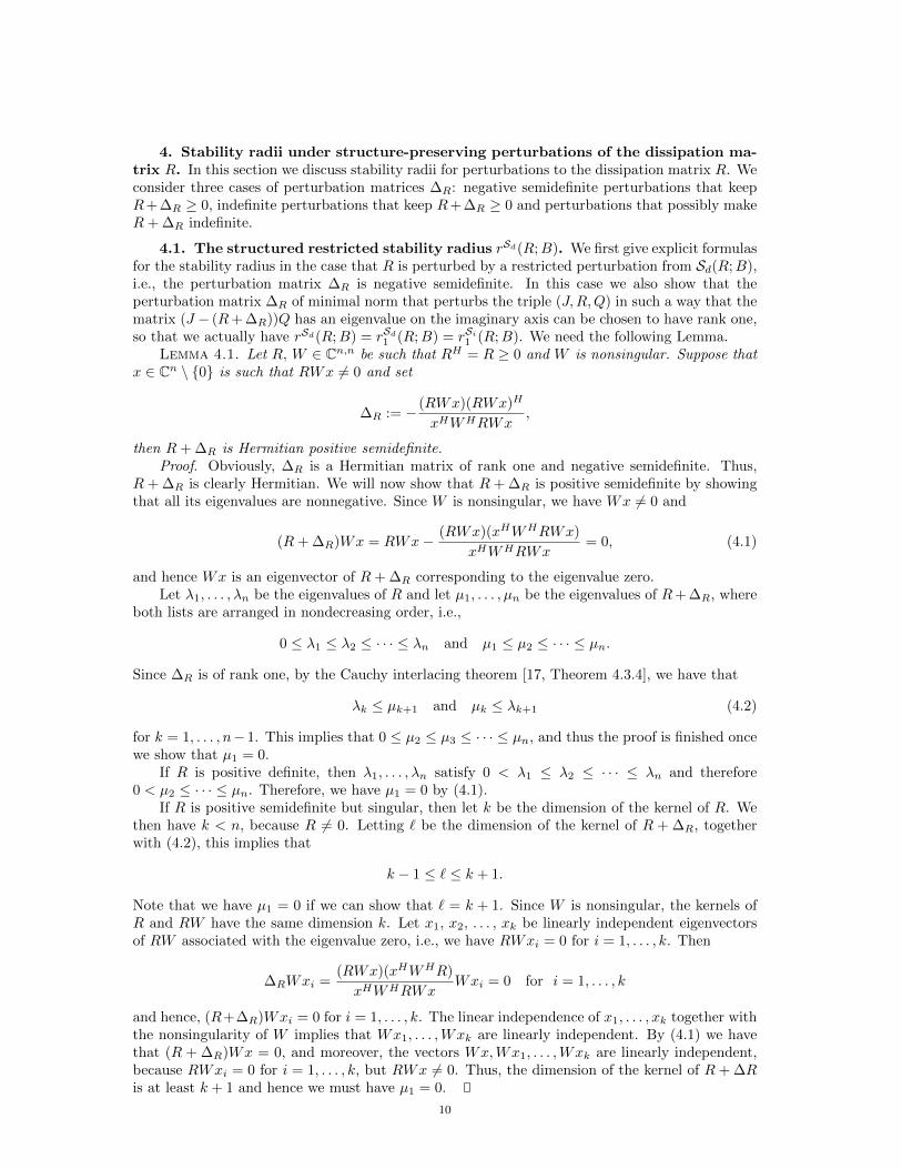
4.1. The structured restricted stability radius rSd(R;B). We first give explicit formulasfor the stability radius in the case that R is perturbed by a restricted perturbation from Sd(R;B),i.e., the perturbation matrix ∆R is negative semidefinite. In this case we also show that theperturbation matrix ∆R of minimal norm that perturbs the triple (J,R,Q) in such a way that thematrix (J − (R+ ∆R))Q has an eigenvalue on the imaginary axis can be chosen to have rank one,so that we actually have rSd(R;B) = rSd1 (R;B) = rSi1 (R;B). We need the following Lemma.

Lemma 4.1. Let R, W ∈ Cn,n be such that RH = R ≥ 0 and W is nonsingular. Suppose thatx ∈ Cn \ 0 is such that RWx 6= 0 and set

∆R := − (RWx)(RWx)H

xHWHRWx,

then R+ ∆R is Hermitian positive semidefinite.Proof. Obviously, ∆R is a Hermitian matrix of rank one and negative semidefinite. Thus,

R + ∆R is clearly Hermitian. We will now show that R + ∆R is positive semidefinite by showingthat all its eigenvalues are nonnegative. Since W is nonsingular, we have Wx 6= 0 and

(R+ ∆R)Wx = RWx− (RWx)(xHWHRWx)

xHWHRWx= 0, (4.1)

and hence Wx is an eigenvector of R+ ∆R corresponding to the eigenvalue zero.Let λ1, . . . , λn be the eigenvalues of R and let µ1, . . . , µn be the eigenvalues of R+ ∆R, where

both lists are arranged in nondecreasing order, i.e.,

0 ≤ λ1 ≤ λ2 ≤ · · · ≤ λn and µ1 ≤ µ2 ≤ · · · ≤ µn.

Since ∆R is of rank one, by the Cauchy interlacing theorem [17, Theorem 4.3.4], we have that

λk ≤ µk+1 and µk ≤ λk+1 (4.2)

for k = 1, . . . , n− 1. This implies that 0 ≤ µ2 ≤ µ3 ≤ · · · ≤ µn, and thus the proof is finished oncewe show that µ1 = 0.

If R is positive definite, then λ1, . . . , λn satisfy 0 < λ1 ≤ λ2 ≤ · · · ≤ λn and therefore0 < µ2 ≤ · · · ≤ µn. Therefore, we have µ1 = 0 by (4.1).

If R is positive semidefinite but singular, then let k be the dimension of the kernel of R. Wethen have k < n, because R 6= 0. Letting ` be the dimension of the kernel of R + ∆R, togetherwith (4.2), this implies that

k − 1 ≤ ` ≤ k + 1.

Note that we have µ1 = 0 if we can show that ` = k + 1. Since W is nonsingular, the kernels ofR and RW have the same dimension k. Let x1, x2, . . . , xk be linearly independent eigenvectorsof RW associated with the eigenvalue zero, i.e., we have RWxi = 0 for i = 1, . . . , k. Then

∆RWxi =(RWx)(xHWHR)

xHWHRWxWxi = 0 for i = 1, . . . , k

and hence, (R+∆R)Wxi = 0 for i = 1, . . . , k. The linear independence of x1, . . . , xk together withthe nonsingularity of W implies that Wx1, . . . ,Wxk are linearly independent. By (4.1) we havethat (R + ∆R)Wx = 0, and moreover, the vectors Wx,Wx1, . . . ,Wxk are linearly independent,because RWxi = 0 for i = 1, . . . , k, but RWx 6= 0. Thus, the dimension of the kernel of R + ∆Ris at least k + 1 and hence we must have µ1 = 0.

10

As a consequence of Lemma 4.1 we obtain the formula for the stability radius rSd(R,B) forperturbations in R that preserve positive semidefiniteness.

Theorem 4.2. Consider an asymptotically stable DH system of the form (1.3) and let thematrix B ∈ Cn,r have full rank r. Then rSd(R,B) is finite if and only if BB†RQx = RQx forsome eigenvector x of JQ. If this is case, then we have

rSd(R;B) = minx∈Ω

∥∥∥∥ (B†RQx)(B†RQx)H

xHQRQx

∥∥∥∥, (4.3)

where Ω is the set of eigenvectors of JQ with the property BB†RQx = RQx.Proof. By definition we have

rSd(R;B) := inf‖∆R‖

∣∣∣ ∆R ∈ Sd(R,B), Λ((J −R)Q− (B∆RB

H)Q)∩ iR 6= ∅

.

Since for ∆R ∈ Sd(R,B) the perturbed matrix R+B∆BH is, by definition of Sd(R,B), Hermitianpositive semidefinite, we obtain by using Lemma 3.1 that

rSd(R;B)

= inf‖∆R‖

∣∣∣ ∆R ∈ Sd(R,B), (R+B∆RBH)Qx = 0 for some eigenvector x of JQ

= inf

‖∆R‖

∣∣∣ ∆R ∈ Sd(R,B), B∆RBHQx = −RQx for some eigenvector x of JQ

= inf

‖∆R‖

∣∣∣ ∆R ∈ Sd(R,B), ∆RBHQx = −B†RQx for some x ∈ Ω

, (4.4)

because by Lemma 2.8 we have B∆RBHQx = −RQx if and only if ∆RB

HQx = −B†RQx andBB†RQx = RQx. From (4.4) and Sd(R,B) ⊆

∆ ∈ Cr,r

∣∣∆H = ∆ ≤ 0

we obtain

rSd(R;B) ≥ inf‖∆‖

∣∣∣ ∆ ∈ Cr,r, ∆H = ∆ ≤ 0, ∆(BHQx) = −B†RQx for some x ∈ Ω. (4.5)

The infimum on the right hand side of (4.5) is finite. Indeed, in view of Remark 2.5 this followsfrom Theorem 2.3, because for x satisfying BB†(RQx) = RQx there exist ∆ ≤ 0 such that∆(BHQx) = −B†RQx if and only if xHQHBB†RQx > 0. Clearly, we have

xHQHBB†RQx = xHQHRQx ≥ 0,

because R is positive semidefinite. Now if 0 = xHQHRQx for some x ∈ Ω then the positivesemidefiniteness of R implies RQx = 0 and thus we have (J − R)Qx = JQx. This implies thatx is an eigenvector of (J − R)Q associated with an eigenvalue on the imaginary axis which is acontradiction to the assumption that (1.3) is asymptotically stable.

Our next step is to show that we have equality in (4.5). Using mappings of minimal normfrom Theorem 2.3 in (4.5) and the fact that x ∈ Ω implies BB†(RQx) = RQx, we obtain

rSd(R;B) ≥ inf‖∆‖

∣∣ ∆ ∈ Cr,r, ∆H = ∆ ≤ 0, ∆(BHQx) = −B†RQx for some x ∈ Ω

= inf

∥∥∥∥ (B†RQx)(B†RQx)H

xHQHBB†RQx

∥∥∥∥∣∣∣∣∣ x ∈ Ω

= infx∈Ω

∥∥∥∥ (B†RQx)(B†RQx)H

xHQRQx

∥∥∥∥. (4.6)

Since we can scale vectors x ∈ Ω to norm one without changing the quotient of norms in (4.6),a compactness argument shows that the infimum is actually a minimum and attained for somex = x. Then setting

∆R := − (B†RQx)(B†RQx)H

xHQRQx,

11

we can show that equality holds in (4.5) if we prove that (R + B∆RBH) is positive semidefinite,

because in that case we have ∆R ∈ Sd(R,B). But this follows from Lemma 4.1 by noting thatBB†RQx = RQx and

R+B∆RBH = R−B

((B†RQx)(B†RQx)H

xHQRQxH

)BH

= R− (BB†RQx)(BB†RQx)H

xHQRQxH

= R− (RQx)(RQx)H

xHQRQxH.

Remark 4.3. It follows from the proof of Theorem 4.2 that the desired perturbation ∆R

of minimal norm can be chosen to be of rank one. Since on the other hand any Hermitianmatrix of rank one is necessarily semi-definite and as discussed in the introduction only a negativesemidefinite Hermitian matrix ∆R in

(J−(R+B∆RB

H)Q can move eigenvalues of (J−R)Q to the

right, we see that any Hermitian rank one perturbation ∆R of (J−R)Q such that(J−(R+∆R)

)Q

has an eigenvalue on the imaginary axis is necessarily negative semidefinite and thus has a normof at least rSd(R;B). Consequently, we have

rSd(R;B) = rSd1 (R;B) = rSi1 (R;B).

In this subsection we have discussed negative semidefinite perturbation matrices ∆R and shownthat the minimal perturbation that moves an eigenvalue to the imaginary axis is achieved by arank one perturbation. In the next section we discuss indefinite perturbation matrices ∆R.

4.2. The stability radius rSi(R;B). This subsection is devoted to the computation of thestability radius rSi(R;B), where the perturbation matrix ∆R is now assumed to be only Hermitian,but not necessarily negative semidefinite. We still require that the system stays DH though, i.e.,that R + B∆RB

H ≥ 0. To derive the formula for rSi(R;B), we employ the Hermitian mappingproblem from Theorem 2.1 and we will use the following lemma.

Lemma 4.4. Let R, ∆R ∈ Herm(n) be such that R > 0 and such that ∆R has at most onenegative eigenvalue. If R+ ∆R is singular then R+ ∆R ≥ 0.

Proof. Let λ1, . . . , λn be the eigenvalues of ∆R. As ∆R has at most one negative eigenvalue,we may assume that λ2, . . . , λn ≥ 0, and we have the spectral decomposition

∆R =n∑j=1

λiuiuHi

with unit norm vectors u1, . . . , un. Clearly, then

R := R+

n∑j=2

λiuiuHi > 0.

Since λ1u1uH1 is of rank one, we can apply the Cauchy interlacing theorem [17, Theorem 4.3.4],

and obtain that R + ∆R = R + λ1u1uH1 has at least n − 1 positive eigenvalues, and hence the

singularity of R+ ∆R implies that R+ ∆R ≥ 0.Theorem 4.5. Consider an asymptotically stable DH system of the form (1.3), let B ∈ Cn,r

have full rank r, and let Ω be the set of eigenvectors x of JQ such that BB†RQx = RQx.1) If R > 0, then rSi(R;B) is finite if and only if Ω 6= ∅. In that case we have

rSi(R;B) = minx∈Ω

‖(B†RQx)‖‖BHQx‖

. (4.7)

2) If R ≥ 0 is singular and if rSi(R;B) is finite, then we have Ω 6= ∅ and

rSi(R;B) ≥ minx∈Ω

‖(B†RQx)‖‖BHQx‖

. (4.8)

12

Proof. By definition, we have

rSi(R;B) := inf‖∆R‖

∣∣∣ ∆R ∈ Si(R,B), Λ((J −R)Q− (B∆RB

H)Q)∩ iR 6= ∅

.

Using Lemma 3.1 and Lemma 2.8, following the lines of the proof of Theorem 4.2 we get

rSi(R;B) = inf‖∆R‖

∣∣∣ ∆R ∈ Si(R,B), ∆R(BHQx) = −B†RQx for some x ∈ Ω.

Since Si(R,B) ⊆ Herm(r), we obtain

rSi(R;B) ≥ inf‖∆R‖

∣∣∣ ∆R ∈ Cr,r, ∆HR = ∆R, ∆R(BHQx) = −B†RQx for some x ∈ Ω

.

(4.9)If Ω 6= ∅, then the finiteness of the right hand side in (4.9) follows from Theorem 2.1 as there exist∆ ∈ Herm(r) such that ∆BHQx = −B†RQx if and only if xHQHBB†RQx ∈ R. This conditionis satisfied, because of the fact that BB†RQx = RQx and because R is Hermitian.

If rSi(R;B) is finite, then Ω 6= ∅, because otherwise the right hand side of (4.9) would beinfinite. Then, using mappings of minimal spectral norm from Theorem 2.1, we obtain

rSi(R;B) ≥ inf‖∆‖

∣∣∣ ∆ ∈ Herm(r), ∆(BHQx) = −B†RQx for some x ∈ Ω

= inf

‖B†RQx‖‖BHQx‖

∣∣∣∣ x ∈ Ω

=‖B†RQx‖‖BHQx‖

, (4.10)

for some x ∈ Ω (again using a compactness argument as in the proof of Theorem 4.2). This proves2) and the inequality ≥ in (4.7). It remains to show that equality holds in (4.10) when R > 0.This would prove (4.7), and also that the non-emptyness of Ω implies that rSi(R;B) is finite.

Thus, assume that R > 0 and let ∆R ∈ Herm(r) be such that

∆R(BHQx) = −B†RQx with ‖∆R‖ =‖B†RQx‖‖BHQx‖

. (4.11)

We show that (R+B∆RBH) ≥ 0, because this implies that ∆R is an element of the set Si(R,B).

The matrix H in (2.1) from Theorem 2.1 has at most one negative eigenvalue, since it eitheris a matrix of rank one or two, and if it has rank two, then it is easy to check that y± (‖y‖/‖x‖)xare eigenvectors of H associated with the eigenvalues ±‖y‖/‖x‖, respectively. This implies that

also B∆RBH has at most one negative eigenvalue. By using (4.11), we furthermore obtain

(R+B∆RBH)Qx = RQx−BB†RQx = RQx−RQx = 0,

because x satisfies BB†RQx = RQx. This implies that R + B∆RBH is singular and thus

Lemma 4.4 yields that (R+B∆RBH) ≥ 0 as desired.

Numerical experiments suggest that the lower bound in (4.8) is actually equal to the structuredstability radius rSi(R;B). We make the following conjecture.

Conjecture 4.6. Consider an asymptotically stable DH system of the form (1.3), let B ∈Cn,r have full rank r, and let z ∈ Cn \ 0 be an eigenvector of JQ such that RQz 6= 0 and

BB†RQz = RQz. Define x := BHQz‖BHQz‖ and y := − B†RQz

‖BHQz‖ and for this choice of x and y let H

be defined by (2.1). Then R+BHBH is a Hermitian positive semidefinite matrix.So far we considered Hermitian perturbations to R, but we required that R + B∆RB

H ≥ 0,to preserve the property that we have a DH system. In Example 1.1, the perturbation that leadsto disk brake squeal, however, is such that R +B∆RB

H is indefinite. Thus, while the symmetrystructures are retained, the system is not DH anymore. It would be conceivable that in this casethe stability radius r(R;B,C) for general perturbations is the relevant quantity. However, as wewill show in the next section, we may still get a larger distance.

13

4.3. The stability radius rHerm(R;B). To derive an explicit formula for the distance

rHerm(R;B) = infω∈R

ηHerm(R;B, iω),

we use the backward error ηHerm(R;B, iω) which can be derived from [19, Theorem 6.2]. We onlystate the parts of that result that are necessary for this paper and remind the reader, that λmin(H)stands for the smallest (possibly negative) eigenvalue of a Hermitian matrix H.

Theorem 4.7 ([19]). Let H0, H1 ∈ Herm(n). Then

infyHH0y

∣∣ y ∈ Cn, ‖y‖ = 1, yHH1y = 0

= supt∈R

λmin(H0 + tH1).

In particular, this value is finite if and only if H1 is not (positive or negative) definite.We first employ this result to compute the eigenvalue backward error ηHerm(R;B, λ) under

Hermitian perturbations to R. The following easy observation will be important when doing so.Remark 4.8. Let W ∈ Cn,n be nonsingular and let B ∈ Cn,r have full rank r. Then it follows

easily by considering the singular value decomposition of B that the dimension of the kernel of(In −BB†)W is r.

Theorem 4.9. Consider a DH system of the form (1.3), let B ∈ Cn,r have full rank r, andlet λ ∈ C be such that W := (J − R)Q − λIn is nonsingular. Furthermore, let the columns ofU ∈ Cn,r form an orthonormal basis of the kernel of (In − BB†)W . Then BHQU is invertible.Furthermore, let L be the Cholesky factor of UHQBBHQU and define the matrices

H0 := B†WUL−H , H1 := L−1UHQWUL−H ,

as well as

H(λ)0 := HH

0 H0, H(λ)1 := i(H1 − HH

1 ).

Then we have

ηHerm(R;B, λ) =

√supt∈R

λmin

(H

(λ)0 + tH

(λ)1

). (4.12)

In particular, ηHerm(R;B, λ) is finite if and only if H(λ)1 is not (positive or negative) definite.

Proof. The dependence on λ in the matrices H(λ)0 and H

(λ)1 has been highlighted for the ease

of future reference only, so in the proof, we will use the abbreviations H0 and H1, respectively.By definition, we have

ηHerm(R;B, λ)

= inf‖∆‖

∣∣∣∆ ∈ Herm(r), λ ∈ Λ(JQ− (R+B∆BH)Q

)= inf

‖∆‖

∣∣∣∆ ∈ Herm(r), x ∈ Cn \ 0,(JQ− (R+B∆BH)Q

)x = λx

= inf

‖∆‖

∣∣∣∆ ∈ Herm(r), x ∈ Cn \ 0, B∆BHQx = Wx

= inf‖∆‖

∣∣∣∆ ∈ Herm(r), x ∈ Cn \ 0, (In −BB†)Wx = 0, ∆BHQx = B†Wx

= inf‖∆‖

∣∣∣∆ ∈ Herm(r), α ∈ Cr \ 0, ∆BHQUα = B†WUα,

where we have used Lemma 2.8 in the second last equality.By using the minimal spectral norm Hermitian mapping from Theorem 2.1 and the fact that

for any x, y ∈ Cn \ 0 there exist ∆ ∈ Herm(r) such that ∆x = y if and only if xHy ∈ R, itfollows that

(ηHerm(R;B, λ)

)2= inf

‖B†WUα‖2

‖BHQUα‖2

∣∣∣∣∣ α ∈ Cr \ 0, αHUHQHWUα ∈ R

. (4.13)

14

Note that BHQU is invertible. Indeed, if we would have BHQUα = 0 for some α ∈ Cr \ 0,then B†WUα = ∆BHQUα = 0 which, together with (In −BB†)WUα = 0, implies WUα = 0 incontradiction to the fact that W is nonsingular. Setting y = LHα in (4.13), we get

(ηHerm(R;B, λ)

)2= inf

yHHH

0 H0y

yHy

∣∣∣∣ y ∈ Cr \ 0, yHH1y ∈ R

, (4.14)

where H0 = B†WUL−H and H1 = L−1UHQWUL−H . Observe that in (4.14) we have yHH1y ∈ Rif and only if yHH1y = 0. Thus, we have(

ηHerm(R;B, λ))2

= inf

yHH0y

yHy

∣∣∣∣ y ∈ Cr \ 0, yHH1y = 0

= sup

t∈Rλmin

(H0 + tH1

),

where the last equality follows from Theorem 4.7.Theorem 4.9 gives us the possibility to characterize the distance rHerm(R;B) for the case that

iJ is indefinite. (Note that this is the case when J is assumed to be real).Corollary 4.10. Consider an asymptotically stable DH system of the form (1.3), where in

addition iJ is indefinite. Let B ∈ Cn,r have full rank r. Then rHerm(R;B) is finite and we have

rHerm(R;B) = infω∈R

√supt∈R

λmin

(H

(iω)0 + tH

(iω)1

), (4.15)

with H(λ)0 , H

(λ)1 as introduced in Theorem 4.9 for a given value λ ∈ C.

Proof. The formula follows immediately from Theorem 4.9. Thus, it remains to show thatrHerm(R;B) is finite, which is the case if the supremum in (4.15) is finite for at least one value

of ω. For this, we have to check that H(iω)1 is not definite for at least one value of ω. But this

follows, because by Theorem 4.9, we have

H(iω)1 = iL−1UH

(QW − (QW )H

)UL−H = L−1UH

(2Q(iJ)Q+ 2ωQ

)UL−H .

Since iJ is assumed to be indefinite, it is clear that H(iω)1 is indefinite for ω = 0.

Having characterized the relevant distances under structured perturbations to R, in the nextsection we discuss perturbations to J .

5. Stability radii under structure-preserving perturbations of J . The analysis for thecase that structure-preserving perturbations are carried out to the structure matrix J is somewhatsimpler than in the case of the dissipation matrix R. We have the following theorem.

Theorem 5.1. Consider an asymptotically stable DH system of the form (1.3), let B ∈ Cn,rhave full rank r. Then rS(J ;B) is finite if and only if there exists a nontrivial intersection Ω ofthe kernel of (In − BB†)(iωIn − JQ) and the kernel of RQ for some ω ∈ R. If this is the case,then BHQU has full rank and we have

rS(J ;B) = infω∈R

σmin

(GSJ (ω)

),

with GSJ (ω) := B†(iωIn − JQ)UL−H , where the columns of U form an orthonormal basis for Ωand L is the Cholesky factor of UHQBBHQU .

Proof. By definition we have

rS(J ;B) = inf‖∆‖

∣∣∣ ∆ ∈ SHerm(r), Λ((J +B∆BH)Q−RQ

)∩ iR 6= ∅

.

Applying Lemma 3.1 it follows that

rS(J ;B)

= inf‖∆‖

∣∣∆ ∈ SHerm(r), (J +B∆BH)Qx = λx, RQx = 0, λ ∈ iR, x ∈ Cn \ 0

= inf‖∆‖

∣∣∆ ∈ SHerm(r), B∆BHQx = (λIn − JQ)x, λ ∈ iR, RQx = 0, x 6= 0.. (5.1)

15

Clearly, ifR > 0 then the kernel ofRQ is 0, and by Lemma 3.1 there does not exist ∆ ∈ SHerm(r)such that

((J +B∆BH)−R

)Q has an eigenvalue on the imaginary axis and hence rS(J ;B) =∞.

Thus, for the remainder of the proof we assume that R is singular. For a fixed ω ∈ R define theeigenvalue backward error under perturbations in J by

ηS(J ;B, iω) = inf‖∆‖

∣∣ ∆ ∈ SHerm(r), B∆BHQx = (iωIn − JQ)x,

for some x 6= 0 with RQx = 0 . (5.2)

Inserting (5.2) into (5.1), we obtain

rS(J ;B) = infω∈R

ηS(J ;B, iω), (5.3)

Note that ∆ ∈ Herm(r) if and only if i∆ ∈ SHerm(r). Hence, in view of Lemma 2.7 and 2.8, forany x 6= 0 and ω ∈ R there exist ∆ ∈ SHerm(r) such that (B∆BH)Qx = (iωIn − JQ)x if andonly if

∆BHQx = B†(iωIn − JQ)x and (In −BB†)(iωIn − JQ)x = 0.

Indeed, the condition xHQHBB†(iωIn − JQ)x ∈ iR from Lemma 2.7 is satisfied, because

xHQHBB†(iωIn − JQ)x = xHQH(iωIn − JQ)x

and QH(iωIn − JQ) is skew-Hermitian. Using this in (5.2) we obtain

ηS(J ;B, iω) = inf‖∆‖

∣∣ ∆ ∈ SHerm(r), x ∈ Ω \ 0, ∆BHQx = B†(iωIn − JQ)x

= inf

‖B†(iωIn − JQ)x‖

‖BHQx‖

∣∣∣∣ x ∈ Ω \ 0, (5.4)

where the last equality follows by using the minimal norm mappings from Theorem 2.1 which canbe done since ∆ ∈ Herm(r) if and only if i∆ ∈ SHerm(r). Thus, by (5.3) and (5.4), rS(J ;B) isfinite if and only if ηS(J ;B, iω) is finite for some ω ∈ R, i.e., Ω 6= 0 for some ω ∈ R.

If ηS(J ;B, iω) is finite for some ω ∈ R, then let dim (Ω) = k and let the columns of U ∈ Cn,kform an orthonormal basis for Ω. Then x ∈ Ω \ 0 implies that x = Uα for some α ∈ Ck \ 0.Using this in (5.4), we obtain

ηS(J ;B, iω) = inf

‖B†(iωIn − JQ)Uα‖

‖BHQUα‖

∣∣∣∣ α ∈ Ck \ 0. (5.5)

Note that BHQU is a full rank matrix, because (J − R)Q has no eigenvalues on the imaginaryaxis. Indeed, if we would have BHQUα = 0 for some α ∈ Ck \ 0 then from (5.2) we have0 = B∆BHQUα = (iωIn − JQ)Uα and this implies (J − R)QUα = iωUα, because Uα ∈ Ω,which is a contradiction. Thus let L be the unique Cholesky factor of UHQHBBHQU , then byinserting y = LHα in (5.5) we have

ηS(J ;B, iω) = inf

‖B†(iωIn − JQ)UL−Hy‖

‖y‖

∣∣∣∣ y ∈ Ck \ 0

= σmin

(B†(iωIn − JQ)UL−H

),

and the assertion follows from (5.3).Having obtained the stability radii for structure-preserving perturbations in R and J , in the

next section we finally consider perturbations in Q.

6. Stability radii under structure-preserving perturbations of Q. The case of per-turbations in Q needs somewhat more discussions than the other cases. Considering Example 1.2which has the form Mx = (J − R)x with Q = I, if M was positive definite, then we could makea change of basis and consider the system ξ = (J − R)Qξ, with Q = M−1. However, since M is

16

singular, this formulation can be made only in the restricted system of dynamical equations, i.e.,the part of the system that corresponds to the variables v and iL. The full system of Example 1.2is automatically on the boundary of the stability region, since we can make M invertible andindefinite by an arbitrarily small perturbation, and then also Q−1 = M would be indefinite. Inthe following, however, we do not consider this more general situation of descriptor systems, butdefer this to a subsequent paper.

By definition we have the following relationships between the stability radii and the distancesto singularity for Q:

r(Q;B) ≤ d(Q;B), rSd(Q;B) ≤ dSd(Q;B) and rSi(Q;B) ≤ dSi(Q;B). (6.1)

So let us first consider the singularity distances.

6.1. The distances to singularity. The following easy observation will be important inthe following.

Remark 6.1. Let W ∈ Cn,n be Hermitian positive definite and let B ∈ Cn,r have full rankr. Recall that by Remark 4.8 the dimension of the kernel of (In − BB†)W is r. If the columnsof U ∈ Cn,r form a basis of the kernel of (In −BB†)W , then BHU is invertible. Indeed, supposethat BHUα = 0 for some α ∈ Cr. Since B† = (BHB)−1BH , we obtain B†Uα = 0 which in turnimplies that

αHUHWUα = αHUH(BB†)WUα = αHUH(BB†)HWUα = (BB†Uα)HWUα = 0,

where we have used that Uα is in the kernel of (In − BB†)W . Since W is positive definite, thisimplies that Uα = 0 and thus α = 0.

Theorem 6.2. Let Q ∈ Herm(n) with Q > 0, and let B ∈ Cn,r be such that rank(B) = r. Letthe columns of U ∈ Cn,r form an orthonormal basis of the kernel of (In −BB†)Q. Then we have

dSd(Q;B) =(σmin(B†QUL−H)

)2,

where L is the Cholesky factor of UHQU , and

d(Q;B,BH) = dSi(Q;B) = σmin(B†QUL−H),

where L is the Cholesky factor of UHBBHU .Proof. In the following we will denote the kernel of (I −BB†)Q by Ω.Concerning the first part of the theorem, we have by definition that

dSd(Q;B) = inf‖∆‖

∣∣ ∆ ∈ Sd(Q,B), det(Q+B∆BH) = 0

= inf‖∆‖

∣∣ ∆ ∈ Sd(Q,B), x ∈ Cn \ 0, (Q+B∆BH)x = 0

= inf‖∆‖

∣∣ ∆ ∈ Sd(Q,B), x ∈ Cn \ 0, B∆BHx = −Qx

≥ inf‖∆‖

∣∣ ∆ ∈ Herm(r), ∆ ≤ 0, x ∈ Cn \ 0, B∆BHx = −Qx, (6.2)

where the last inequality holds, because Sd(Q,B) ⊆ ∆ ∈ Herm(r) | ∆ ≤ 0. By Lemma 2.8 wehave B∆BHx = −Qx if and only if ∆BHx = −B†Qx and BB†Qx = Qx. Note that the lattercondition is already sufficient for the existence of a matrix ∆H = ∆ ≤ 0 such that ∆BHx =−B†Qx. Indeed, the necessary condition −xHBB†Qx < 0 in Lemma 2.6 is automatically satisfiedbecause BB†Qx = Qx and because Q is Hermitian positive definite. Using this observationin (6.2), we obtain

dSd(Q;B) ≥ inf‖∆‖

∣∣∣ ∆ ∈ Herm(r), ∆ ≤ 0, x ∈ Cn \ 0,

∆BHx = −B†Qx, BB†Qx = Qx

(6.3)

= inf

‖(B†Qx)(B†Qx)H‖

‖xHQx‖

∣∣∣∣ x ∈ Ω \ 0, (6.4)

17

where the last equality follows by using minimal spectral norm mappings from Theorem 2.3.We aim to show that equality holds in (6.3). To this end, note again that x can be scaled

to norm one, and thus a compactness argument shows that the infimum in (6.4) is actually aminimum. Thus, let x ∈ Ω be such that

‖(B†Qx)(B†Qx)H‖‖xHQx‖

= inf

‖(B†Qx)(B†Qx)H‖

‖xHQx‖

∣∣∣∣ x ∈ Ω \ 0

and define

∆ := − (B†Qx)(B†Qx)H

xHQx,

so that we have ∆BH x = −B†Qx. Equality holds in (6.3) if we show that (Q + B∆BH) ≥ 0,

because this will imply that ∆ ∈ Sd(Q,B). Since B∆BH is of rank one, it has at most onenegative eigenvalue. Furthermore, we have

(Q+B∆BH)x = Qx−BB†Qx = Qx−Qx = 0,

and thus, (Q+B∆BH) ≥ 0 by Lemma 4.4. Therefore we have equality in (6.3), i.e.,

dSd(Q;B) = inf

‖B†Qx‖2

xHQx

∣∣∣∣ x ∈ Ω \ 0

= inf

‖B†QUα‖2

αHUHQUα

∣∣∣∣ α ∈ Cr \ 0, (6.5)

where the columns of U ∈ Cn,r form an orthonormal basis for Ω. Let L be the unique Choleskyfactor of UHQU > 0, then inserting y = LHα in (6.5), we get

dSd(Q;B) = inf

‖B†QUL−Hy‖2

‖y‖2

∣∣∣∣ y ∈ Cr \ 0

=(σmin(B†QUL−H)

)2.

which proves the first part of the assertion.For the second part, again by definition, we have

dSi(Q;B) := inf‖∆‖

∣∣ ∆ ∈ Si(Q,B), det(Q+B∆BH) = 0.

Following the steps of the first part, we have

dSi(Q;B) ≥ inf‖∆‖

∣∣ ∆ ∈ Herm(r), x ∈ Cn \ 0, ∆BHx = −B†Qx, BB†Qx = Qx

= inf

‖B†Qx‖‖BHx‖

∣∣∣∣ x ∈ Ω \ 0, (6.6)

where the last equality follows by using the minimal spectral norm mappings of Theorem 2.1. Letx ∈ Ω \ 0 be such that

‖B†Qx‖‖BH x‖

= inf

‖B†Qx‖‖BHx‖

∣∣∣ 0 6= x ∈ Ω

(again the infimum is a minimum and thus attained) and let ∆ ∈ Herm(r) be the corresponding

minimal norm mapping such that ‖∆‖ := ‖B†Qx‖‖BH x‖ and ∆BH x = −B†Qx. Then we have equality

in (6.6) if we show that (Q + B∆BH) ≥ 0, because this will imply that ∆ ∈ Si(Q,B). But this

follows from Lemma 4.4, because ∆ is either a matrix of rank one or an indefinite matrix of ranktwo. Thus,

dSi(Q;B) = inf

‖B†Qx‖‖BHx‖

∣∣∣ x ∈ Ω \ 0

= inf

‖B†QUα‖‖BHUα‖

∣∣∣∣ α ∈ Cr \ 0, (6.7)

18

where columns of U ∈ Cn,r form an orthonormal basis for Ω. By Remark 6.1 the matrix BHU isinvertible. Thus, let L be the Cholesky factor of UHBBHU . By inserting y = LHα in (6.7), weobtain

dSi(Q;B) = inf

‖B†QUL−Hy‖

‖y‖

∣∣∣∣ y ∈ Ck \ 0

= σmin(B†QUL−H).

It remains to show that d(Q;B,BH) = dSi(Q;B). By definition, we have

d(Q;B,BH) = inf‖∆‖

∣∣ ∆ ∈ Cr,r, det(Q+B∆BH) = 0

= inf‖∆‖

∣∣ ∆ ∈ Cr,r, x ∈ Cn \ 0, (Q+B∆BH)x = 0

= inf‖∆‖

∣∣∆ ∈ Cr,r, x ∈ Ω \ 0, ∆BHx = −B†Qx, (6.8)

where the last equality holds due to Lemma 2.8. Note that by [39], for any x, y ∈ Cn, x 6= 0 wehave

inf‖∆‖

∣∣ ∆x = y

=‖y‖‖x‖

.

Using this in (6.8), we obtain

d(Q;B,BH) = inf

‖B†Qx‖‖BHx‖

∣∣∣∣ x ∈ Ω \ 0

= dSi(Q;B),

where the last equality follows from (6.7). Therefore we have

d(Q;B,BH) = dSi(Q;B) = σmin(B†QUL−H).

After characterizing the distances to singularity, in the next subsections we characterize thestability radii.

6.2. The stability radius rSi(Q;B). For the characterization of rSi(Q;B) we have thefollowing theorem.

Theorem 6.3. Consider an asymptotically stable DH system of the form (1.3), let B ∈ Cn,rhave full rank r, and let dSi(Q;B) be as in Theorem 6.2. If R > 0, then

rSi(Q;B) = dSi(Q;B).

Furthermore, if R ≥ 0 is singular, let R be the set of all ω ∈ R \ 0 such that the intersectionof the kernel ΩR of R and the kernel Ωω of (I −BB†)(iωIn − JQ) is not the zero space, and foreach ω ∈ R let the columns of Vω form an orthonormal basis for ΩR ∩Ωω. Then BHJVω has fullcolumn rank for all ω ∈ R. If

infω∈R

σmin

(B†(iωIn −QJ)VωL

−Hω

),

is attained for some ω ∈ R, where Lω is the Cholesky factor of V Hω JHBBHJVω, then

rSi(Q;B) = mindSi(Q;B), inf

ω∈Rσmin

(B†(iωIn −QJ)VωL

−Hω

). (6.9)

Proof. If R > 0, then by definition

rSi(Q;B) = inf‖∆‖

∣∣∣ ∆ ∈ Si(Q,B), Λ((J −R)(Q+B∆BH)

)∩ iR 6= ∅

.

Observe that in this case zero is the only choice to move an eigenvalue of (J−R)Q to the imaginaryaxis, and the way to achieve this is to make Q singular, because for any W ∈ Herm(r) if Q+W

19

is nonsingular, then R(Q+W )x 6= 0 for any x ∈ Cn \ 0. Thus by Lemma 3.1, (J −R)(Q+W )cannot have any nonzero eigenvalues on the imaginary axis. With this observation we obtain

rSi(Q;B) = inf‖∆‖

∣∣∣ ∆ ∈ Si(Q,B), Λ((J −R)(Q+B∆BH)

)∩ 0 6= ∅

= inf

‖∆‖

∣∣∣ ∆ ∈ Si(Q,B), det(Q+B∆BH) = 0, (6.10)

where the last equality holds, because J −R is invertible, since (J −R)Q is nonsingular, becauseit has no eigenvalues on the imaginary axis. Therefore, from (6.10) we have

rSi(Q;B) = dSi(Q;B).

Next, we consider the case that R ≥ 0 is singular. By definition of Si(Q,B) we have

Si(Q,B) =

∆ ∈ Herm(r)∣∣ (Q+B∆BH) ≥ 0

,

and (Q + B∆BH) ≥ 0 if and only if either (Q + B∆BH) ≥ 0 and det(Q + B∆BH) = 0, or(Q+B∆BH) > 0. Thus, we can write

rSi(Q;B) = min

inf‖∆‖

∣∣ ∆ ∈ Herm(r), (Q+B∆BH) ≥ 0, det(Q+B∆BH) = 0,

Λ((J −R)(Q+B∆BH)

)∩ iR 6= ∅

,

inf‖∆‖

∣∣ ∆ ∈ Herm(r), (Q+B∆BH) > 0,

Λ((J −R)(Q+B∆BH)

)∩ iR 6= ∅

. (6.11)

For the first of the two infima in (6.11), we have

inf‖∆‖

∣∣ ∆ ∈ Herm(r), (Q+B∆BH) ≥ 0, det(Q+B∆BH) = 0,

Λ((J −R)(Q+B∆BH)

)∩ iR 6= ∅

= inf

‖∆‖

∣∣∣ ∆ ∈ Herm(r), (Q+B∆BH) ≥ 0, det(Q+B∆BH) = 0

= dSi(Q;B),

because Λ((J −R)(Q+B∆BH)

)∩ iR 6= ∅ is automatically satisfied if det(Q+B∆BH) = 0. For

the second of the two infima in (6.11), using Lemma 3.1 we obtain that

inf‖∆‖

∣∣∣ ∆ ∈ Herm(r), (Q+B∆BH) > 0, Λ((J −R)(Q+B∆BH)

)∩ iR 6= ∅

= inf

‖∆‖

∣∣∣∆ ∈ Herm(r), (Q+B∆BH) > 0, ω ∈ R \ 0, x ∈ Cn \ 0,

J(Q+B∆BH)x = iωx and R(Q+B∆BH)x = 0

= inf‖∆‖

∣∣∣ ∆ ∈ Herm(r), (Q+B∆BH) > 0, ω ∈ R \ 0, y ∈ Cn \ 0,

(Q+B∆BH)Jy = iωy and Ry = 0

= inf‖∆‖

∣∣∣ ∆ ∈ Herm(r), (Q+B∆BH) > 0, ω ∈ R \ 0, y ∈ Cn \ 0,

B∆BHJy = (iωIn −QJ)y and Ry = 0

= infω∈R

inf‖∆‖

∣∣∣ ∆ ∈ Herm(r), (Q+B∆BH) > 0, y ∈ Cn \ 0,

B∆BHJy = (iωIn −QJ)y and Ry = 0

≥ infω∈R

inf‖∆‖

∣∣∣ ∆ ∈ Herm(r), y ∈ ΩR \ 0, B∆BHJy = (iωIn −QJ)y, (6.12)

20

where in the second equality, we replaced (Q + B∆BH)x with y using the nonsingularity ofQ + B∆BH , and for the last step we used ∆ ∈ Herm(r) | (Q + B∆BH) > 0 ⊆ Herm(r). ByLemma 2.7, for any y ∈ Cn \ 0 there exist ∆ ∈ Herm(r) such that B∆BHJy = (iωIn −QJ)y ifand only if BB†(iωIn −QJ)y = (iωIn −QJ)y. Indeed, note that the condition

yHJHBB†(iωIn −QJ)y ∈ R (6.13)

in Lemma 2.7 is automatically satisfied due to the fact that BB†(iωIn − QJ)y = (iωIn − QJ)yand that JH(iωIn −QJ) is Hermitian. Using this in (6.12) and applying Lemma 2.8, we get

inf‖∆‖

∣∣∣ ∆ ∈ Herm(r), (Q+B∆BH) > 0, Λ((J −R)(Q+B∆BH)

)∩ iR 6= ∅

≥ infω∈R

inf‖∆‖

∣∣∣ ∆ ∈ Herm(r), y ∈ ΩR \ 0, ∆BHJy = B†(iωIn −QJ)y,

BB†(iωIn −QJ)y = (iωIn −QJ)y

(6.14)

= infω∈R

inf

‖B†(iωIn −QJ)y‖

‖BHJy‖

∣∣∣∣ y ∈ (ΩR ∩ Ωω) \ 0

= infω∈R

inf

‖B†(iωIn −QJ)Vωα‖

‖BHJVωα‖

∣∣∣∣ α ∈ Ckω \ 0, (6.15)

where for ω ∈ R, i.e., ω 6= 0 and ΩR ∩Ωω 6= 0, the columns of Vω ∈ Cn,kω form an orthonormalbasis of ΩR ∩Ωω, and we have set y = Vωα for some α ∈ Ckω \ 0. Note that for the second lastequality we have used the minimal spectral norm mappings from Theorem 2.1.

Furthermore, we have BHJy 6= 0 for all y ∈ (ΩR∩Ωω)\0 and therefore also BHJVωα 6= 0 forall α ∈ Ckω \0, and thus BHJVω has full rank. Indeed, if BHJy = 0 for some y ∈ ΩR∩Ωω thenby (6.14) we have B†(iωIn −QJ)y = 0 and thus also BB†(iωIn −QJ)y = 0. Since y ∈ Ωω, i.e., yis in the kernel of (I −BB†)(iωIn−JQ), it follows that 0 = (iωIn−QJ)y =

(iωIn−Q(J −R)

)y,

which is a contradiction to the fact that (J − R)Q has no eigenvalues on the imaginary axis.Therefore, V Hω JHBBHJVω has a unique Cholesky factor Lω, and setting β = LHω α in (6.15), weobtain

inf‖∆‖

∣∣∣ ∆ ∈ Herm(r), (Q+B∆BH) > 0, Λ((J −R)(Q+B∆BH)

)∩ iR 6= ∅

≥ infω∈R

inf

‖B†(iωIn −QJ)VωL

−Hω β‖

‖β‖

∣∣∣∣ β ∈ Ck \ 0

= infω∈R

σmin

(B†(iωIn −QJ)VωL

−Hω

). (6.16)

By assumption, the infimum in (6.16) is attained for some ω ∈ R. Thus, writing V = Vω and

L = Lω we have that

σ := σmin

(B†(iωIn −QJ)V L−H

)= infω∈R

σmin

(B†(iωIn −QJ)VωL

−Hω

).

Let u be a right singular vector of B†(iωIn − QJ)V L−H corresponding to the minimal singular

value σ and set z := V L−Hu. Furthermore, applying Theorem 2.1 let ∆ ∈ Herm(r) be such that

∆BHJz = B†(iωIn − QJ)z and ‖∆‖ = σmin

(B†(iωIn − QJ)V L−H

). Inserting this in (6.16) we

have

inf‖∆‖

∣∣∣ ∆ ∈ Herm(r), (Q+B∆BH) > 0, Λ((J −R)(Q+B∆BH)

)∩ iR 6= ∅

≥ ‖∆‖.

Then to show (6.9), we consider two cases depending on further properties of the matrix ∆.

If (Q+B∆BH) > 0 then we have equality in (6.16) and therefore

rSi(Q;B) = ‖∆‖ = σmin

(B†(iωIn −QJ)V L−H

).

21

If (Q+B∆BH) has some nonpositive eigenvalues, then

inf‖∆‖

∣∣∣ ∆ ∈ Herm(r), (Q+B∆BH) > 0, Λ((J −R)(Q+B∆BH)

)∩ iR 6= ∅

≥ inf

‖∆‖

∣∣∣ ∆ ∈ Herm(r), (Q+B∆BH) ≥ 0, det(Q+B∆BH) = 0,

Λ((J −R)(Q+B∆BH)

)∩ iR 6= ∅

.

This follows by using the fact that eigenvalues depend continuously on the entries of a matrix andtherefore there exist t ∈ (0, 1] such that (Q + tB∆BH) ≥ 0 and (Q + tB∆BH) is singular. But

this implies that ‖∆‖ ≥ ‖t∆‖ ≥ dSi(Q;B). Thus, we have rSi(Q;B) = dSi(Q;B) in that casewhich finishes the proof.

6.3. The stability radius rSd(Q;B). As final case we obtain the following formula for thestructured restricted stability radius rSd(Q;B).

Theorem 6.4. Consider an asymptotically stable DH system of the form (1.3), let B ∈ Cn,rhave full rank r, and let dSd(Q;B) be as in Theorem 6.2.

If R > 0, then

rSd(Q;B) = dSd(Q;B).

If, however, R ≥ 0 is singular, then let R be the set of all ω ∈ R\0 such that the intersectionof the kernel ΩR of R and the kernel Ωω of (I −BB†)(iωIn −QJ) is not the zero space. Assume

that for every ω ∈ R we have yHJH(iwIn − QJ)y < 0 for all vectors y ∈ (ΩR ∪ Ωω) \ 0.Moreover, for each ω ∈ R let the columns of Vω form an orthonormal basis for ΩR ∩ Ωω. If

infω∈R

(σmin

(B†(iωIn −QJ)VωL

−Hω

))2,

is attained for some ω ∈ R, where Lω is the Cholesky factor of V Hω JH(QJ − iωIn)Vω, then

rSd(Q;B) = mindSd(Q;B), inf

ω∈R

(σmin

(B†(iωIn −QJ)VωL

−Hω

))2 .

Proof. The proof is analogous to the proof of Theorem 6.3, by using Theorem 2.3 instead ofTheorem 2.1. The difference is that condition (6.13) becomes yHJH(iωIn−QJ)y < 0 which is nolonger automatically satisfied and thus, leads to a further assumption in the definition of the setR.

7. Numerical experiments. In this section, we present some numerical experiments toillustrate the results of this paper and to show that the stability radii are indeed larger whenstructure-preserving perturbations are considered instead of general ones, and this difference canbe significant. To compute the distances, in all cases we used the function fminsearch in MatlabVersion No. 7.8.0 (R2009a) to solve the associated optimization problems, except for the compu-tation of rHerm(R;B), where we first used the software package CVX [12] for the inner supremumand then the function fminsearch for the outer infimum.

In all our numerical experiments, we chose random matrices J, R, Q, B ∈ Cn,n for differentvalues of n ≤ 9 with JH = −J, RH = R ≥ 0 and QH = Q > 0 and B of full rank, such that allrestricted stability radii were finite.

The computed stability radii rSd(R;B) and rSi(R;B) with respect to structured restrictedperturbations to R are as obtained in Theorem 4.2 and 4.5, respectively, rS(J ;B) with respectto structured restricted perturbations to J is as obtained in Theorem 5.1, and rSi(Q;B) andrSd(Q;B) with respect to structured restricted perturbations to Q are as obtained in Theorem 6.3and 6.4, respectively. The structured distances to singularity dSi(Q;B), dSd(Q;B) are as obtainedin Theorem 6.2.

22

size n r(R;B,BH) rHerm(R;B) rSi(R;B) rSd(R;B)3 0.2985 0.2985 2.7154 11.36934 0.0826 0.4704 1.1527 1.95715 3.3358 3.4302 4.0866 6.06526 0.5919 0.6020 2.6858 6.46747 0.0675 0.1048 0.9606 6.03108 1.5933 1.6193 14.7738 20.51059 1.4520 1.4524 16.4666 29.0445

Table 7.1Unstructured and various structured stability radii when perturbing only R.

The unstructured and various structured stability radii with respect to structure-preservingrestricted perturbations to R are depicted in Table 7.1. As mentioned in Section 4 earlier, Conjec-ture 4.6 holds in all our numerical experiments, so the lower bounds in Theorem 4.5 indeed gavethe values of rSi(R;B).

In Table 7.2, we compare various stability radii. The results illustrate that stability radii withrespect to perturbations to only Q are much smaller than the other stability radii. In some casesthe stability radius rSi(Q;B) is even smaller than the stability radius r(J ;B,BH). Table 7.2 alsoexhibits the difference between the stability radii rS(J ;B) and rSi(R;B).

size n r(Q;B,BH) rSi(Q;B) r(J ;B,BH) rS(J ;B) rSi(R;B)= dSi(Q;B) = r(R;B,BH)

3 0.1608 0.1751 0.3427 2.5123 0.90284 0.0101 0.0119 0.2054 2.2756 1.62065 0.0485 0.1191 0.1391 2.2292 1.20256 0.0129 0.0132 0.1763 2.2127 5.12377 0.0736 0.0813 0.0747 1.8043 4.17888 0.0021 0.0025 0.1154 2.2579 1.68389 0.0074 0.0076 0.0913 3.0741 2.8177

Table 7.2Comparison of various structured stability radii.

In our numerical experiments we found several instances of randomly generated matricesJ, R, Q and B for which structured stability radii with respect to restricted perturbations to Qare significantly smaller than the structured restricted distances to singularity for Q. The valuesfor a few such cases are reported in Table 7.3.

size n r(Q;B,BH) rSi(Q;B) dSi(Q;B) rSd(Q;B) dSd(Q;B)3 0.0031 0.1310 0.2079 0.1988 0.20794 0.0776 0.2308 0.2571 0.2404 0.25715 0.0014 0.0649 0.1287 0.1104 0.12876 0.0262 0.0731 0.1068 0.0923 0.10687 0.0071 0.0276 0.0355 0.0290 0.03558 0.0022 0.0163 0.0257 0.0224 0.02579 0.0055 0.0263 0.0424 0.0371 0.0424

Table 7.3Unstructured and various structured stability radii while perturbing only Q.

Example 7.1. To illustrate the distance to instability in the case that R is perturbed to beindefinite, consider again Example 1.1 and the first order formulation (1.4) and write R = R1 +R2,

23

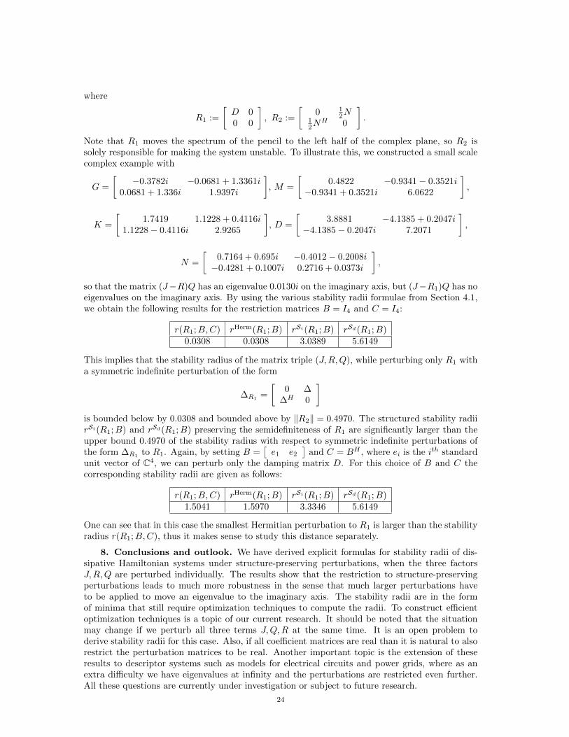
where

R1 :=

[D 00 0

], R2 :=

[0 1

2N12N

H 0

].

Note that R1 moves the spectrum of the pencil to the left half of the complex plane, so R2 issolely responsible for making the system unstable. To illustrate this, we constructed a small scalecomplex example with

G =

[−0.3782i −0.0681 + 1.3361i

0.0681 + 1.336i 1.9397i

], M =

[0.4822 −0.9341− 0.3521i

−0.9341 + 0.3521i 6.0622

],

K =

[1.7419 1.1228 + 0.4116i

1.1228− 0.4116i 2.9265

], D =

[3.8881 −4.1385 + 0.2047i

−4.1385− 0.2047i 7.2071

],

N =

[0.7164 + 0.695i −0.4012− 0.2008i−0.4281 + 0.1007i 0.2716 + 0.0373i

],

so that the matrix (J−R)Q has an eigenvalue 0.0130i on the imaginary axis, but (J−R1)Q has noeigenvalues on the imaginary axis. By using the various stability radii formulae from Section 4.1,we obtain the following results for the restriction matrices B = I4 and C = I4:

r(R1;B,C) rHerm(R1;B) rSi(R1;B) rSd(R1;B)0.0308 0.0308 3.0389 5.6149

This implies that the stability radius of the matrix triple (J,R,Q), while perturbing only R1 witha symmetric indefinite perturbation of the form

∆R1=

[0 ∆

∆H 0

]is bounded below by 0.0308 and bounded above by ‖R2‖ = 0.4970. The structured stability radiirSi(R1;B) and rSd(R1;B) preserving the semidefiniteness of R1 are significantly larger than theupper bound 0.4970 of the stability radius with respect to symmetric indefinite perturbations ofthe form ∆R1 to R1. Again, by setting B =

[e1 e2

]and C = BH , where ei is the ith standard

unit vector of C4, we can perturb only the damping matrix D. For this choice of B and C thecorresponding stability radii are given as follows:

r(R1;B,C) rHerm(R1;B) rSi(R1;B) rSd(R1;B)1.5041 1.5970 3.3346 5.6149

One can see that in this case the smallest Hermitian perturbation to R1 is larger than the stabilityradius r(R1;B,C), thus it makes sense to study this distance separately.

8. Conclusions and outlook. We have derived explicit formulas for stability radii of dis-sipative Hamiltonian systems under structure-preserving perturbations, when the three factorsJ,R,Q are perturbed individually. The results show that the restriction to structure-preservingperturbations leads to much more robustness in the sense that much larger perturbations haveto be applied to move an eigenvalue to the imaginary axis. The stability radii are in the formof minima that still require optimization techniques to compute the radii. To construct efficientoptimization techniques is a topic of our current research. It should be noted that the situationmay change if we perturb all three terms J,Q,R at the same time. It is an open problem toderive stability radii for this case. Also, if all coefficient matrices are real than it is natural to alsorestrict the perturbation matrices to be real. Another important topic is the extension of theseresults to descriptor systems such as models for electrical circuits and power grids, where as anextra difficulty we have eigenvalues at infinity and the perturbations are restricted even further.All these questions are currently under investigation or subject to future research.

24

REFERENCES

[1] A.C. Antoulas. Approximation of large-scale dynamical systems, volume 6 of Advances in Design and Control.Society for Industrial and Applied Mathematics (SIAM), Philadelphia, PA, 2005.

[2] S. Bora, M. Karow, C. Mehl, and P. Sharma. Structured eigenvalue backward errors of matrix pencils andpolynomials with Hermitian and related structures. SIAM J. Matrix Anal. Appl., 35(2):453–475, 2014.

[3] R. Byers. A bisection method for measuring the distance of a stable to unstable matrices. SIAM J. Sci.Statist. Comput., 9:875–881, 1988.

[4] S. L. Campbell. Linearization of DAEs along trajectories. Z. Angew. Math. Phys., 46:70–84, 1995.[5] M. Dalsmo and A.J. van der Schaft. On representations and integrability of mathematical structures in

energy-conserving physical systems. SIAM J. Control Optim., 37:54–91, 1999.[6] D. Estevez-Schwarz and C. Tischendorf. Structural analysis for electrical circuits and consequences for MNA.

Internat. J. Circ. Theor. Appl., 28:131–162, 2000.[7] M.A. Freitag and A. Spence. A Newton-based method for the calculation of the distance to instability. Linear

Algebra Appl., 435(12):3189–3205, 2011.[8] R. W. Freund. The sprim algorithm for structure-preserving order reduction of general rcl circuits. In M. Hinze

P. Benner and J.W. ter Maten, editors, Model reduction for circuit simulation, Lecture Notes in ElectricalEngineering, pages 25–52. Springer-Verlag, Berlin, Germany, 2011.

[9] G. Golo, A.J. van der Schaft, P.C. Breedveld, and B.M. Maschke. Hamiltonian formulation of bond graphs. InA. Rantzer R. Johansson, editor, Nonlinear and Hybrid Systems in Automotive Control, pages 351–372.Springer-Verlag, Heidelberg, Germany, 2003.

[10] G. H. Golub and C. F. Van Loan. Matrix Computations. Johns Hopkins Univ. Press, Baltimore, 3rd edition,1996.

[11] N. Grabner, V. Mehrmann, S. Quraishi, C. Schroder, and U. von Wagner. Numerical methods for parametricmodel reduction in the simulation of disc brake squeal. To appear in Z. Angew. Math. Mech., 2016.

[12] M. Grant and S. Boyd. Cvx: Matlab software for disciplined convex programming, version 2.0 beta.http://cvxr.com/cvx, September 2012.

[13] C. He and G.A. Watson. An algorithm for computing the distance to instability. SIAM J. Matrix Anal. Appl.,20(1):101–116, 1998.

[14] D. Hinrichsen and A. J. Pritchard. Stability radii of linear systems. Systems Control Lett., 7:1–10, 1986.[15] D. Hinrichsen and A. J. Pritchard. Real and complex stability radii: a survey. In Control of uncertain systems,

pages 119–162, Birkhauser, Boston, MA, USA, 1990.[16] D. Hinrichsen and A. J. Pritchard. Mathematical Systems Theory I. Modelling, State Space Analysis, Stability

and Robustness. Springer-Verlag, New York, NY, 2005.[17] R. A. Horn and C. R. Johnson. Matrix Analysis. Cambridge University Press, Cambridge, 1985.[18] B. Jacob and H. Zwart. Linear port-Hamiltonian systems on infinite-dimensional spaces. Operator Theory:

Advances and Applications, 223. Birkhauser/Springer Basel AG, Basel CH, 2012.[19] M. Karow. µ-values and spectral value sets for linear perturbation classes defined by a scalar product. SIAM

J. Matrix Anal. Appl., 32:845–865, 2011.[20] P. Kunkel and V. Mehrmann. Differential-Algebraic Equations. Analysis and Numerical Solution. EMS

Publishing House, Zurich, Switzerland, 2006.[21] P. Lancaster and M. Tismenetsky. The Theory of Matrices. Academic Press, Orlando, 2nd edition, 1985.[22] D.S. Mackey, N. Mackey, and F. Tisseur. Structured mapping problems for matrices associated with scalar

products. Part i: Lie and Jordan algebras. SIAM J. Matrix Anal. Appl., 29(4):1389–1410, 2008.[23] N. Martins. Efficient eigenvalue and frequency response methods applied to power system small-signal stability

studies. IEEE Trans. on Power Systems, 1:217–224, 1986.[24] N. Martins and L. Lima. Determination of suitable locations for power system stabilizers and static var

compensators for damping electromechanical oscillations in large scale power systems. IEEE Trans. onPower Systems, 5:1455–1469, 1990.

[25] N. Martins, P.C. Pellanda, and J. Rommes. Computation of transfer function dominant zeros with applicationsto oscillation damping control of large power systems. IEEE Trans. on Power Systems, 22:1657–1664,2007.

[26] B.M. Maschke, A.J. van der Schaft, and P.C. Breedveld. An intrinsic Hamiltonian formulation of networkdynamics: non-standard poisson structures and gyrators. J. Franklin Inst., 329:923–966, 1992.

[27] A. J. Mayo and A. C. Antoulas. A framework for the solution of the generalized realization problem. LinearAlgebra Appl., 425:634–662, 2007.

[28] R. Ortega, A.J. van der Schaft, Y. Mareels, and B.M. Maschke. Putting energy back in control. Control Syst.Mag., 21:18–33, 2001.

[29] R. Ortega, A.J. van der Schaft, B.M. Maschke, and G. Escobar. Interconnection and damping assignmentpassivity-based control of port-controlled Hamiltonian systems. Automatica, 38:585–596, 2002.

[30] J. Rommes and N. Martins. Exploiting structure in large-scale electrical circuit and power system problems.Linear Algebra Appl., 431:318–333, 2009.

[31] A.J. van der Schaft. Port-Hamiltonian systems: an introductory survey. In J.L. Verona M. Sanz-Sole andJ. Verdura, editors, Proc. of the International Congress of Mathematicians, vol. III, Invited Lectures,pages 1339–1365, Madrid, Spain.

[32] A.J. van der Schaft. Port-Hamiltonian systems: network modeling and control of nonlinear physical systems.In Advanced Dynamics and Control of Structures and Machines, CISM Courses and Lectures, Vol. 444.

25

Springer Verlag, New York, N.Y., 2004.[33] A.J. van der Schaft. Port-Hamiltonian differential-algebraic systems. In Surveys in Differential-Algebraic

Equations, pages 173–226. Springer, 2013.[34] A.J. van der Schaft and B.M. Maschke. The Hamiltonian formulation of energy conserving physical systems

with external ports. Arch. Elektron. Ubertragungstech., 45:362–371, 1995.[35] A.J. van der Schaft and B.M. Maschke. Hamiltonian formulation of distributed-parameter systems with

boundary energy flow. J. Geom. Phys., 42:166–194, 2002.[36] A.J. van der Schaft and B.M. Maschke. Port-Hamiltonian systems on graphs. SIAM J. Control Optim., 2013.[37] W. Schiehlen. Multibody Systems Handbook. Springer-Verlag, Heidelberg, Germany, 1990.[38] J.-G. Sun. Backward perturbation analysis of certain characteristic subspaces. Numer. Math., 65:357–382,

1993.[39] G. Trenkler. Matrices which take a given vector into a given vector-revisited. Amer. Math. Monthly, 111:50–52,

2004.[40] C.F. Van Loan. How near is a matrix to an unstable matrix? Contemp. Math. AMS, 47:465–479, 1984.[41] K. Veselic. Damped oscillations of linear systems: a mathematical introduction. Springer-Verlag, Heidelberg,

2011.

26