lab 2.pdf

ECS 701 Communication Theory

Lab Session: Wireless communication systems simulation using MATLAB

2. Digital Modulation

November 2013

1 FSK Digital Modulation

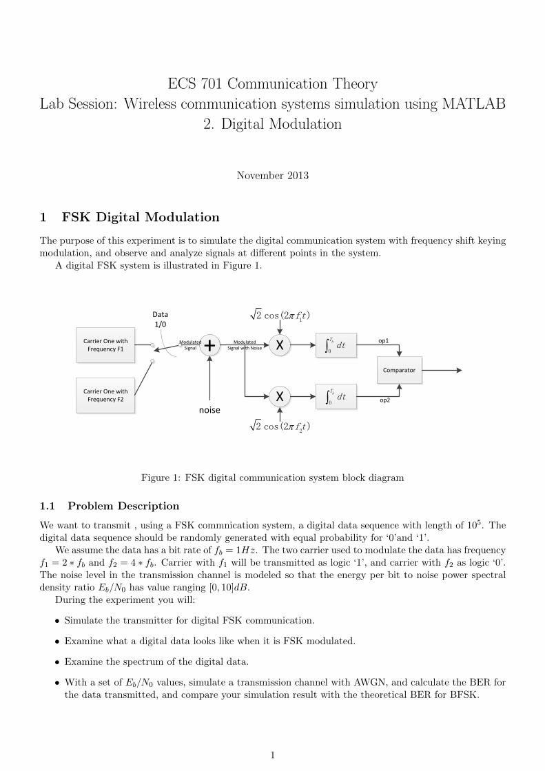
The purpose of this experiment is to simulate the digital communication system with frequency shift keyingmodulation, and observe and analyze signals at different points in the system.

A digital FSK system is illustrated in Figure 1.

Carrier One with Frequency F1

Carrier One with Frequency F2

+

noise

ModulatedSignal

Data1/0

X

X

ModulatedSignal with Noise

Comparator

op1

op2

0

bTdt

0

bTdt

12 cos(2 )ft

22 cos(2 )ft

Figure 1: FSK digital communication system block diagram

1.1 Problem Description

We want to transmit , using a FSK commnication system, a digital data sequence with length of 105. Thedigital data sequence should be randomly generated with equal probability for ‘0’and ‘1’.

We assume the data has a bit rate of fb = 1Hz. The two carrier used to modulate the data has frequencyf1 = 2 ∗ fb and f2 = 4 ∗ fb. Carrier with f1 will be transmitted as logic ‘1’, and carrier with f2 as logic ‘0’.The noise level in the transmission channel is modeled so that the energy per bit to noise power spectraldensity ratio Eb/N0 has value ranging [0, 10]dB.

During the experiment you will:

• Simulate the transmitter for digital FSK communication.

• Examine what a digital data looks like when it is FSK modulated.

• Examine the spectrum of the digital data.

• With a set of Eb/N0 values, simulate a transmission channel with AWGN, and calculate the BER forthe data transmitted, and compare your simulation result with the theoretical BER for BFSK.

1

1.2 Experiment Process

1.2.1 Initilizing the parameters

Open a new MATLAB description file, and insert the following code. Note the choosing of samplingfrequency.

%% intialization of parameters

N = 1e5; % Number of symbols simulating

Tb = 1; % Symbol duration 1 sec

f1 = 1/Tb * 2; % Frequency of first carrier

f2 = 1/Tb * 4; % Frequency of second carrier

fs = 4*f2; % Sampling frequency

M = fs/Tb; % Number of samples per symbol

t = 0:1/fs:N*Tb;

After that, save the script and name it as “FSK.m”. Run the script by entering FSK in the MATLABcommand window.

1.2.2 Simulation of FSK transmitter

At a FSK transmitter, you will firstly need to randomly generate a sequence of digital data. i.e. [1,0,0,0,1,1,0,1,...];With the data, you then need to convert it to an actual time domain base band digital signal, in other words,represent each digital symbol using a set of samples. Then you will need to modulate the data using FSK.This is done using simple selection as described in Figure 1.

Insert the following code to the MATLAB script and save and run it.

% Generate Original baseband data, 1, 0 with equal probability

data = round(rand(1, N));

base_band_signal = zeros(1, length(t));

for jj = 1:N

if data(jj)

base_band_signal((1:M)+M*(jj-1)) = 1;

end

end

% Modulate the data using FSK

modulated_signal = zeros(1, length(t));

for jj = 1:N

if data(jj)

modulated_signal((1:M)+M*(jj-1)) = (sqrt(2)/sqrt(Tb))*cos(2*pi*f1.*t(1:M));

else

modulated_signal((1:M)+M*(jj-1)) = (sqrt(2)/sqrt(Tb))*cos(2*pi*f2.*t(1:M));

end

end

1.2.3 Examine the baseband signal and modulated signal

We will firstly look at the signal in time domain. Enter the following commands in the command window.Note that we are only looking at a short segment of the signals, not the whole signal, because there are 105

bits in total.

2

figure

subplot(2,1,1)

plot(t(1:100), base_band_signal(1:100))

title('Base Band Digital Signal');

xlabel('Time');

subplot(2,1,2)

plot(t(1:100), modulated_signal(1:100))

title('Modulated FSK Signal');

xlabel('Time');

Now we will examine the spectrum characteristics of a digital signal and the FSK modulated digitalsignal. Enter the following commands in the command window.

figure

n = 2^(nextpow2(length(base_band_signal)));

BBS = fft(base_band_signal, n)/fs;

df = fs/n;

f = (0:df:df*(n-1)) -fs/2;

subplot(2,1,1)

semilogy(f, fftshift(abs(BBS)))

axis([-5 5 0.001 1000])


xlabel('Frequency');

MS = fft(modulated_signal, n)/fs;

subplot(2,1,2)

semilogy(f, fftshift(abs(MS)))

axis([0 8 1e-4 1e3])



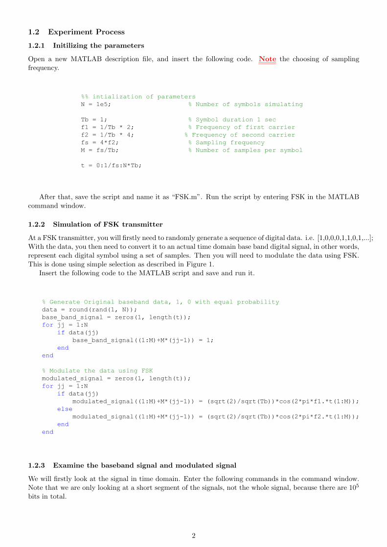
Note the spectrum characteristics of a digital signal. This type of spectrum is very oftenly seen whenusing a spectrum analyzer to observe a digital signal. See Figure below as an example.

Figure 2: Typical output of a spectrum analyzer

3

1.2.4 Simulation of transmission channel

The simplest channel model for simulation and anaslysis is a Additive White Gaussian Noise AWGN channel.And this is what we are going to do here.

We need to calculate the actual noise signal (with correct variance) satisfying a given Eb/N0 value. Andthe noise signal is added to the modulated signal (Additive Noise).

Insert the following code to the matlab script and save it.

%% At the transmission channel

% calculate noise that is added to the transmitted signal

EbNo_dB = 0;

% white gaussian noise with 0dB variance

noise = 1/sqrt(2)*(randn(1,length(t)) +1i*rand(1, length(t)));

% Actual noise satisfying required EbNo value

snr = 10.^(EbNo_dB/10)*(1/Tb)/fs;

actual_noise = noise./sqrt(snr);

received_signal = modulated_signal + actual_noise;

1.3 Simulation of FSK receiver

We use coherrent FSK receiver to demodulate the received signal. Insert the following code to the matlabscript.

%% At the Receiver side

% coherent receiver

op1 = conv(received_signal, (sqrt(2)/sqrt(Tb))*cos(2*pi*f1.*t(1:M)));

op2 = conv(received_signal, (sqrt(2)/sqrt(Tb))*cos(2*pi*f2.*t(1:M)));

% demodulation

demodulated_data = [real(op1(M+1:M:end)) > real(op2(M+1:M:end))];

Err = demodulated_data - data;

Now you can examine whether there is a transmission error due to noisy channel by checking the contentof vector Err. If there is a detection error, the value of the corresponding bit in vector Err will have a non-zeros value. Check the first 20 value of Err by entering Err(1:20) in the command wnidow.

1.3.1 Bit Error Rate simulation and analysis

Now we will try to simulate the transmission process with different value of Eb/N0 and evaluate the BERby counting the detection errors.

To do this, you need to modify the structure of your MATLAB script so that the simulation is repeatedin iterations. Modify your code so that it looks like:

4

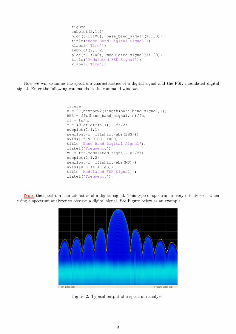
%% Initialization of parameters

% this is same as before

% ADD here a initilization of EbNo vectors

EbNo_dB = 0:10;

% ADD the iteration code

for ii = 1:length(EbNo_dB)

%% original Transmitter code

%% channel simulation code

% remove the original code : EbNo_dB = 0;

% modify snr = 10.^(EbNo_dB/10)*(1/Tb)/fs;

snr = 10.^(EbNo_dB(ii)/10)*(1/Tb)/fs;

% This is trying to give EbNo a different value in each iteration

%% Receiver code

% ADD the following code at the end to record the number of errors

nErr(ii) = length(find(Err ~= 0));

end

%Calculate the BER result from simulation

ber_simulation = nErr/N;

%Calculate the theoretical BER for BFSK

ber_theory = 0.5*erfc(sqrt((10.^(EbNo_dB/10))/2));

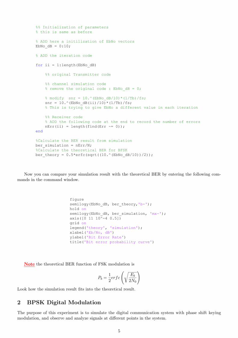
Now you can compare your simulation result with the theoretical BER by entering the following com-mands in the command window.

figure

semilogy(EbNo_dB, ber_theory,'b-');

hold on

semilogy(EbNo_dB, ber_simulation, 'mx-');

axis([0 11 10^-4 0.5])

grid on

legend('theory', 'simulation');

xlabel('Eb/No, dB')

ylabel('Bit Error Rate')

title('Bit error probability curve')

Note the theoretical BER function of FSK modulation is

Pb =1

2erfc

(√Eb

2N0

)Look how the simulation result fits into the theoretical result.

2 BPSK Digital Modulation

The purpose of this experiment is to simulate the digital communication system with phase shift keyingmodulation, and observe and analyze signals at different points in the system.

5

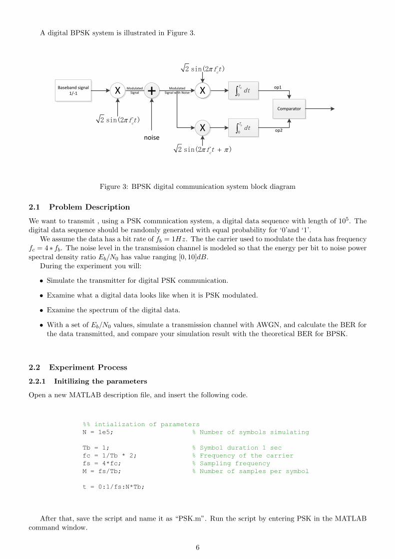
A digital BPSK system is illustrated in Figure 3.

+

noise

ModulatedSignal X

X

ModulatedSignal with Noise

Comparator

op1

op2

0

bTdt

0

bTdt

2 sin(2 )cft

2 sin(2 )cft

Baseband signal1/-1 XX

2 sin(2 )cft

Figure 3: BPSK digital communication system block diagram


We want to transmit , using a PSK commnication system, a digital data sequence with length of 105. Thedigital data sequence should be randomly generated with equal probability for ‘0’and ‘1’.

We assume the data has a bit rate of fb = 1Hz. The the carrier used to modulate the data has frequencyfc = 4 ∗ fb. The noise level in the transmission channel is modeled so that the energy per bit to noise powerspectral density ratio Eb/N0 has value ranging [0, 10]dB.


• Simulate the transmitter for digital PSK communication.

• Examine what a digital data looks like when it is PSK modulated.

• Examine the spectrum of the digital data.

• With a set of Eb/N0 values, simulate a transmission channel with AWGN, and calculate the BER forthe data transmitted, and compare your simulation result with the theoretical BER for BPSK.



Open a new MATLAB description file, and insert the following code.

%% intialization of parameters

N = 1e5; % Number of symbols simulating

Tb = 1; % Symbol duration 1 sec

fc = 1/Tb * 2; % Frequency of the carrier

fs = 4*fc; % Sampling frequency

M = fs/Tb; % Number of samples per symbol

t = 0:1/fs:N*Tb;

After that, save the script and name it as “PSK.m”. Run the script by entering PSK in the MATLABcommand window.

6

2.2.2 Simulation of PSK transmitter

At a FSK transmitter, you will firstly need to randomly generate a sequence of digital data. i.e. [1,0,0,0,1,1,0,1,...];The simplest way to modulate a PSK signal is to multiply the carrier with 1 and -1 for logical 0 and 1, sothat they have a 180◦ phase shift.


%% At the Transmitter side

% Generate Original baseband data, 1, 0 with equal probability

data = round(rand(1, N));

base_band_signal = zeros(1, length(t));

for jj = 1:N

if data(jj)

base_band_signal((1:M)+M*(jj-1)) = 1;

end

end

base_band_signal = base_band_signal * 2 - 1;

% Modulate the data using PSK

modulated_signal = base_band_signal .* (sqrt(2)/sqrt(Tb)).* sin(2*pi*fc.*t);

2.2.3 Examine the baseband signal and modulated signal

We will firstly look at the signal in time domain. Enter the following commands in the command window.Note the difference of modulated PSK and FSK signals. Also Note the 180 degree phase shift of the signalwhen the data switches between 0 and 1.

figure

subplot(2,1,1)

plot(t(1:100), base_band_signal(1:100))


xlabel('Time');

subplot(2,1,2)

plot(t(1:100), modulated_signal(1:100))

title('Modulated PSK Signal');

xlabel('Time');

Now we will examine the spectrum characteristics of a digital signal and the PSK modulated digitalsignal. Enter the following commands in the command window.

7

figure

n = 2^(nextpow2(length(base_band_signal)));

BBS = fft(base_band_signal, n)/fs;

df = fs/n;

f = (0:df:df*(n-1)) -fs/2;

subplot(2,1,1)

semilogy(f, fftshift(abs(BBS)))

axis([-5 5 0.001 1000])



MS = fft(modulated_signal, n)/fs;

subplot(2,1,2)

semilogy(f, fftshift(abs(MS)))







%% At the transmission channel

% calculate noise that is added to the transmitted signal

EbNo_dB = 0;

% white gaussian noise with 0dB variance

noise = 1/sqrt(2)*(randn(1,length(t)) +1i*rand(1, length(t)));

% Actual noise satisfying required EbNo value

snr = 10.^(EbNo_dB/10)*(1/Tb)/fs;

actual_noise = noise./sqrt(snr);

received_signal = modulated_signal + actual_noise;

2.3 Simulation of PSK receiver

We use coherrent PSK receiver to demodulate the received signal. Insert the following code to the matlabscript.

% coherent receiver

op1 = conv(received_signal, (sqrt(2)/sqrt(Tb)).*sin(2*pi*fc.*t(1:M)));

op2 = conv(received_signal, (sqrt(2)/sqrt(Tb)).*(-1)*sin(2*pi*fc.*t(1:M)));

demodulated_data = [real(op1(M+1:M:end)) < real(op2(M+1:M:end))];

Err = demodulated_data - data;

nErr(ii) = length(find(Err ~= 0));

Now you can examine whether there is a transmission error due to noisy channel by checking the content

8

of vector Err. If there is a detection error, the value of the corresponding bit in vector Err will have a non-zeros value. Check the first 20 value of Err by entering Err(1:20) in the command wnidow.


You will need to perform similar changes to your code structure as in the FSK simulation case. And runyour simulation again. Compare your simulation results with the theoretical BER for BPSK.

Note the theoretical BER function of BPSK modulation is

Pb =1

2erfc

(√Eb

N0


3 QPSK Digital Modulation

The purpose of this experiment is to simulate the digital communication system with phase shift keyingmodulation, and observe and analyze signals at different points in the system. The difference from thissection to the previous example is that we use QPSK (4PSK) to modulate the digital data.

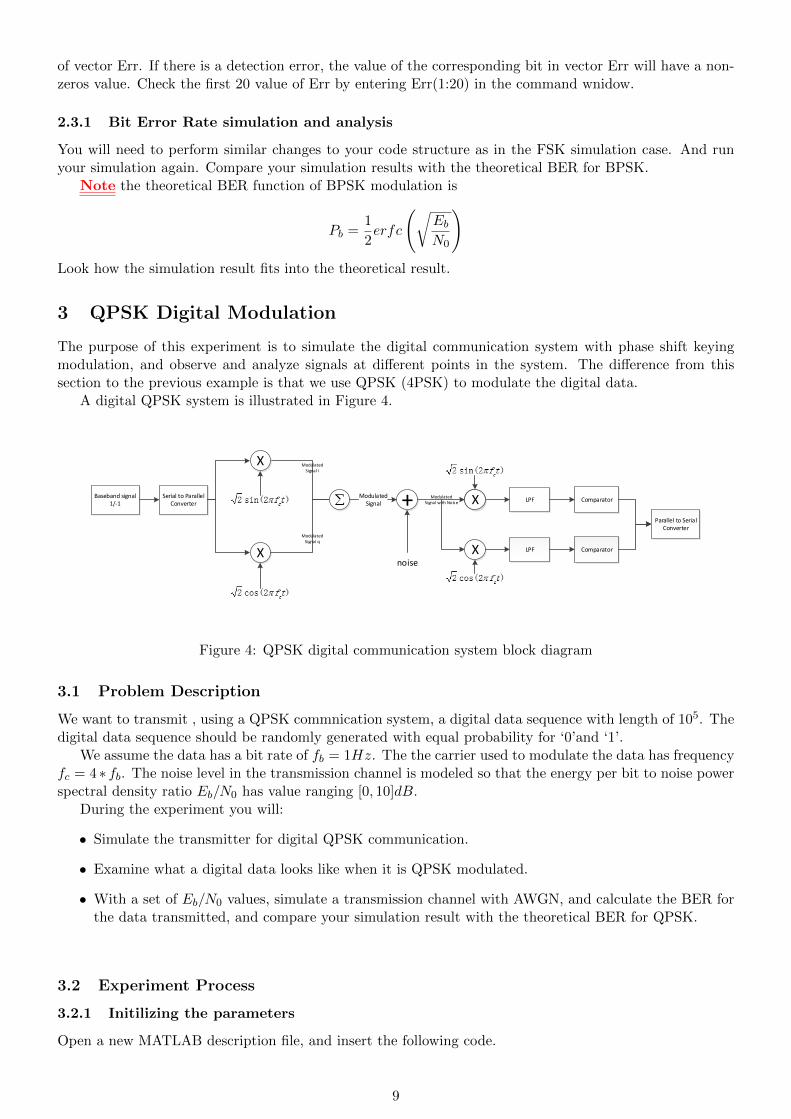
A digital QPSK system is illustrated in Figure 4.

+

noise

ModulatedSignal i

X

X

LPF

LPF

ModulatedSignal with Noise Comparator

Serial to Parallel Converter X

X

X

ModulatedSignal q

Comparator

Baseband signal1/-1

Parallel to Serial Converter

ModulatedSignal

Figure 4: QPSK digital communication system block diagram


We want to transmit , using a QPSK commnication system, a digital data sequence with length of 105. Thedigital data sequence should be randomly generated with equal probability for ‘0’and ‘1’.

We assume the data has a bit rate of fb = 1Hz. The the carrier used to modulate the data has frequencyfc = 4 ∗ fb. The noise level in the transmission channel is modeled so that the energy per bit to noise powerspectral density ratio Eb/N0 has value ranging [0, 10]dB.


• Simulate the transmitter for digital QPSK communication.

• Examine what a digital data looks like when it is QPSK modulated.

• With a set of Eb/N0 values, simulate a transmission channel with AWGN, and calculate the BER forthe data transmitted, and compare your simulation result with the theoretical BER for QPSK.



Open a new MATLAB description file, and insert the following code.

9

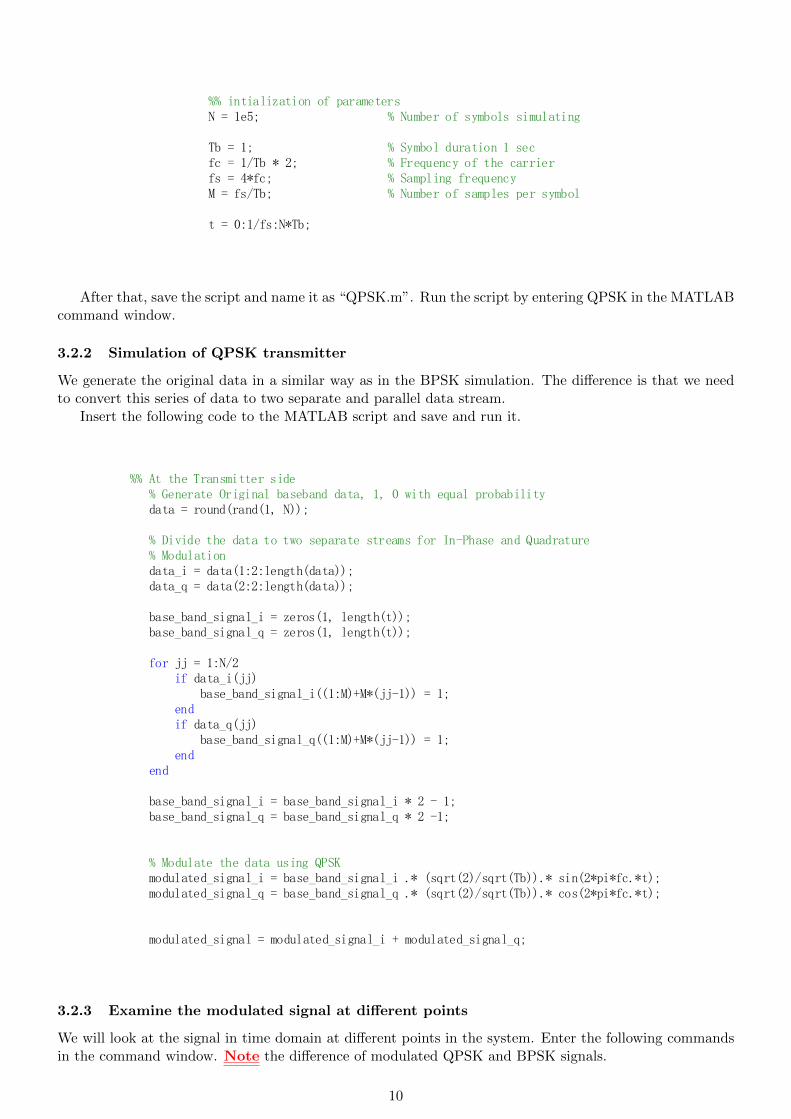
%% intialization of parametersN = 1e5; % Number of symbols simulating Tb = 1; % Symbol duration 1 secfc = 1/Tb * 2; % Frequency of the carrierfs = 4*fc; % Sampling frequencyM = fs/Tb; % Number of samples per symbol t = 0:1/fs:N*Tb;

After that, save the script and name it as “QPSK.m”. Run the script by entering QPSK in the MATLABcommand window.

3.2.2 Simulation of QPSK transmitter

We generate the original data in a similar way as in the BPSK simulation. The difference is that we needto convert this series of data to two separate and parallel data stream.


%% At the Transmitter side % Generate Original baseband data, 1, 0 with equal probability data = round(rand(1, N)); % Divide the data to two separate streams for In-Phase and Quadrature % Modulation data_i = data(1:2:length(data)); data_q = data(2:2:length(data)); base_band_signal_i = zeros(1, length(t)); base_band_signal_q = zeros(1, length(t)); for jj = 1:N/2 if data_i(jj) base_band_signal_i((1:M)+M*(jj-1)) = 1; end if data_q(jj) base_band_signal_q((1:M)+M*(jj-1)) = 1; end end base_band_signal_i = base_band_signal_i * 2 - 1; base_band_signal_q = base_band_signal_q * 2 -1; % Modulate the data using QPSK modulated_signal_i = base_band_signal_i .* (sqrt(2)/sqrt(Tb)).* sin(2*pi*fc.*t); modulated_signal_q = base_band_signal_q .* (sqrt(2)/sqrt(Tb)).* cos(2*pi*fc.*t); modulated_signal = modulated_signal_i + modulated_signal_q;

3.2.3 Examine the modulated signal at different points

We will look at the signal in time domain at different points in the system. Enter the following commandsin the command window. Note the difference of modulated QPSK and BPSK signals.

10

figuresubplot(3,1,1)plot(t(1:100), modulated_signal_i(1:100))title('Modulated PSK Signal: In Phase');xlabel('Time');subplot(3,1,2)plot(t(1:100), modulated_signal_q(1:100))title('Modulated PSK Signal: Quadrature');xlabel('Time');subplot(3,1,3)plot(t(1:100), modulated_signal(1:100))title('Modulated PSK Signal');xlabel('Time');





%% At the transmission channel % calculate noise that is added to the transmitted signal % white gaussian noise with 0dB variance noise = 1/sqrt(2)*(randn(1,length(t)) +1i*rand(1, length(t))); % Actual noise satisfying required EbNo value snr = 10.^(EbNo_dB(ii)/10)*(1/Tb)/fs; actual_noise = noise./sqrt(snr); received_signal = modulated_signal + actual_noise;

3.3 Simulation of QPSK receiver

We use coherrent QPSK receiver to demodulate the received signal. Insert the following code to the matlabscript.

11

%% At the Receiver side % coherent receiver op1 = conv(received_signal, (sqrt(2)/sqrt(Tb)).*sin(2*pi*fc.*t(1:M))); op2 = conv(received_signal, (sqrt(2)/sqrt(Tb)).*(-1)*sin(2*pi*fc.*t(1:M))); demodulated_data_i = [real(op1(M+1:M:end)) < real(op2(M+1:M:end))]; op3 = conv(received_signal, (sqrt(2)/sqrt(Tb)).*cos(2*pi*fc.*t(1:M))); op4 = conv(received_signal, (sqrt(2)/sqrt(Tb)).*(-1)*cos(2*pi*fc.*t(1:M))); demodulated_data_q = [real(op3(M+1:M:end)) > real(op4(M+1:M:end))]; demodulated_data = zeros(1, N); % parallel to serial combining for jj = 1:N/2 demodulated_data(jj*2-1) = demodulated_data_i(jj); demodulated_data(jj*2) = demodulated_data_q(jj); end Err = demodulated_data - data; nErr(ii) = length(find(Err ~= 0));end

Now you can examine whether there is a transmission error due to noisy channel by checking the contentof vector Err. If there is a detection error, the value of the corresponding bit in vector Err will have a non-zeros value. Check the first 20 value of Err by entering Err(1:20) in the command wnidow.


You will need to perform similar changes to your code structure as in the BPSK simulation case. And runyour simulation again. Compare your simulation results with the theoretical BER for BPSK.

Note the theoretical BER function of QPSK modulation is

Pb =1

2erfc

(√Eb

2N0


First DraftB. Zhong. Dec 2012.RevisionB. Zhong. Nov 2013.

12

lab 2.pdf

Documents