laboratory 4: the z –transform

EE-384: Digital Signal Processing Spring 2020

Laboratory 4: The z –transform

Instructor: Mr Ammar Naseer EE UET New Campus

Aims

This lab session provides signal and system description in the complex frequency domain. MATLAB

techniques are introduced to analyze z-transforms and to compute inverse z-transforms. Solutions of

difference equations using the z-transform and MATLAB are also provided.

Pre-Lab:

The z-Transform The z-transform of a sequence x(n) is given by

where z is a complex variable. The set of z values for which X(z) exists is called the region of convergence

(ROC) and is given by

for some non-negative numbers R1 and R2.

The inverse z-transform of a complex function X(z) is given by

where C is a counterclockwise contour encircling the origin and lying in the ROC.

Comments:

1. The complex variable z is called the complex frequency given by | | !, where | | is the

magnitude and is the real frequency.

2. Since the ROC (4.2) is defined in terms of the magnitude | | the shape of the ROC is an open

ring. Note that R1 may be equal to zero and/or R2 could possibly be ∞.

Laboratory 4: The z –transform 4.2

3. If R2 < R1, then the ROC is a null space and the z-transform does not exist.

4. The function | | (or ) is a circle of unit radius in the z-plane and is called the unit

circle. If the ROC contains the unit circle, then we can evaluate X(z) on the unit circle.

Therefore the discrete-time Fourier transform ) may be viewed as a special case of the z-

transform X(z).

Properties of the ROC

Note that the ROC is a distinguishing feature that guarantees the uniqueness of the z- transform. Hence

it plays a very important role in system analysis.

1. The ROC is always bounded by a circle since the convergence condition is on the magnitude | |.

2. The sequence ) ) is a special case of a right-sided sequence, defined as a sequence

x(n) that is zero for some n < n0. The ROC for right-sided sequences is always outside of a circle

of radius R1. If n0 ≥ 0, then the right-sided sequence is also called a causal sequence.

3. The sequence ) ) is a special case of a left-sided sequence, defined as a

sequence x(n) that is zero for some n > n0. If n0 ≥ 0, the resulting sequence is called an anticausal

sequence. The ROC for left-sided sequences is always inside of a circle of radius R2.

4. The ROC for two-sided sequences is always an open ring R1 < | |< R2, if it exists.

5. The sequences that are zero for n < n1 and n > n2 are called finite-duration sequences. The ROC

for such sequences is the entire z-plane. If n1 < 0, then z = 1 is not in the ROC. If n2 > 0, then z = 0

is not in the ROC.

6. The ROC cannot include a pole since X(z) converges uniformly in there.

7. There is at least one pole on the boundary of a ROC of a rational X(z).

8. The ROC is one contiguous region; that is, the ROC does not come in pieces. In digital signal

processing, signals are assumed to be causal since almost every digital data is acquired in real

time. Therefore the only ROC of interest to us is the one given in statement 2.

Important Properties of the z-Transform

We state the following important properties of the z-transform without proof.

1. Linearity:

2. Sample Shifting

3. Frequency Shifting

4. Folding:


5. Complex Conjugation:

6. Differentiation in z-domain:

7. Multiplication:

where C is a closed contour that encloses the origin and lies in the common ROC.

8. Convolution

This last property transforms the time-domain convolution operation into a multiplication between two functions.

It is a significant property in many ways. First, if X1(z) and X2(z) are two polynomials, then their product can be

implemented using the conv function in MATLAB.

Let ) and ) . Determine X3(z) =X1(z)X2(z).

From the definition of the z-transform, we observe that

[ ] [ ] and [ ] [ ]

Then the convolution of these two sequences will give the coefficients of the required polynomial product.

>> x1 = [2,3,4]; >> x2 = [3,4,5,6]; >> x3 = conv(x1,x2) x3 = 6 17 34 43 38 24

Hence

)

Note that using the conv_m function developed in Lab 3, we can also multiply two z-domain polynomials

corresponding to noncausal sequences.

4. A Let ) and ) . Determine X3(z) =X1(z)X2(z).

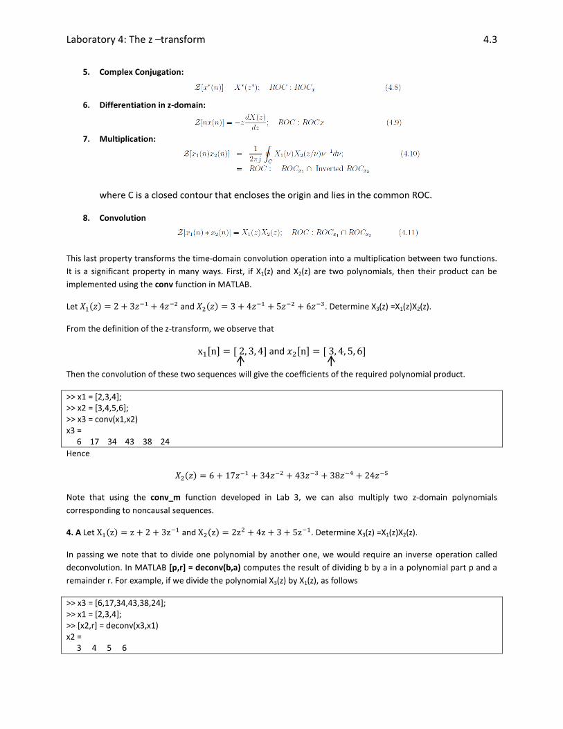
In passing we note that to divide one polynomial by another one, we would require an inverse operation called

deconvolution. In MATLAB [p,r] = deconv(b,a) computes the result of dividing b by a in a polynomial part p and a

remainder r. For example, if we divide the polynomial X3(z) by X1(z), as follows

>> x3 = [6,17,34,43,38,24]; >> x1 = [2,3,4]; >> [x2,r] = deconv(x3,x1) x2 = 3 4 5 6


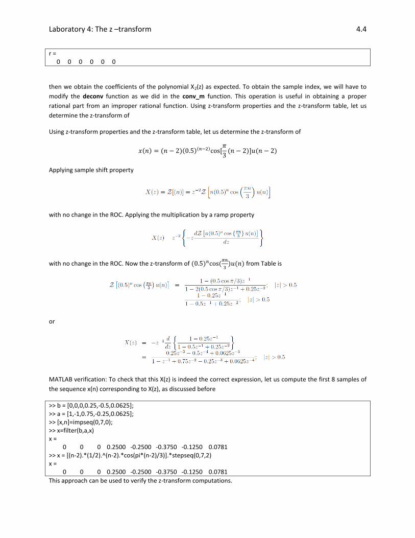
r = 0 0 0 0 0 0

then we obtain the coefficients of the polynomial X2(z) as expected. To obtain the sample index, we will have to

modify the deconv function as we did in the conv_m function. This operation is useful in obtaining a proper

rational part from an improper rational function. Using z-transform properties and the z-transform table, let us

determine the z-transform of

Using z-transform properties and the z-transform table, let us determine the z-transform of

) ) ) ) [

)] )

Applying sample shift property

with no change in the ROC. Applying the multiplication by a ramp property

with no change in the ROC. Now the z-transform of )

) ) from Table is

or

MATLAB verification: To check that this X(z) is indeed the correct expression, let us compute the first 8 samples of

the sequence x(n) corresponding to X(z), as discussed before

>> b = [0,0,0,0.25,-0.5,0.0625]; >> a = [1,-1,0.75,-0.25,0.0625]; >> [x,n]=impseq(0,7,0); >> x=filter(b,a,x) x = 0 0 0 0.2500 -0.2500 -0.3750 -0.1250 0.0781 >> x = [(n-2).*(1/2).^(n-2).*cos(pi*(n-2)/3)].*stepseq(0,7,2) x = 0 0 0 0.2500 -0.2500 -0.3750 -0.1250 0.0781

This approach can be used to verify the z-transform computations.


Inversion of the z-Transform

From equation (4.3), the inverse z-transform computation requires an evaluation of a complex contour

integral that, in general, is a complicated procedure. The most practical approach is to use the partial

fraction expansion method. It makes use of the z-transform table. The z-transform, however, must be a

rational function. This requirement is generally satisfied in digital signal processing.

A MATLAB function residuez is available to compute the residue part and the direct (or polynomial)

terms of a rational function in . Let

be a rational function in which the numerator and the denominator polynomials are in ascending

powers of z-1. Then [R,p,C]=residuez(b,a) computes the residues, poles, and direct terms of X(z) in which

two polynomials B(z) and A(z) are given in two vectors b and a, respectively. The returned column vector

R contains the residues, column vector p contains the pole locations, and row vector C contains the

direct terms. If p(k)=...=p(k+r-1) is a pole of multiplicity r, then the expansion includes the term of the

form

Similarly, [b,a]=residuez(R,p,C), with three input arguments and two output arguments, converts the

partial fraction expansion back to polynomials with coefficients in row vectors b and a.

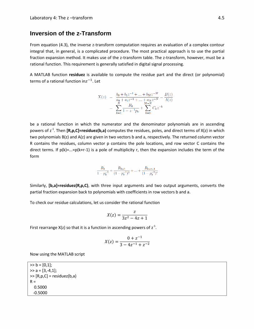
To check our residue calculations, let us consider the rational function

)

First rearrange X(z) so that it is a function in ascending powers of z-1.

)

Now using the MATLAB script

>> b = [0,1]; >> a = [3,-4,1]; >> [R,p,C] = residuez(b,a) R = 0.5000 -0.5000


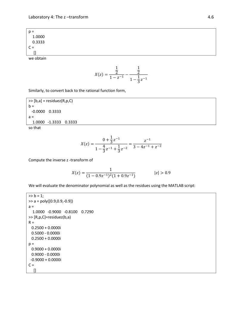
p = 1.0000 0.3333 C = []

we obtain

)

Similarly, to convert back to the rational function form,

>> [b,a] = residuez(R,p,C) b = -0.0000 0.3333 a = 1.0000 -1.3333 0.3333

so that

)

Compute the inverse z -transform of

)

) ) | |

We will evaluate the denominator polynomial as well as the residues using the MATLAB script:

>> b = 1; >> a = poly([0.9,0.9,-0.9]) a = 1.0000 -0.9000 -0.8100 0.7290 >> [R,p,C]=residuez(b,a) R = 0.2500 + 0.0000i 0.5000 - 0.0000i 0.2500 + 0.0000i p = 0.9000 + 0.0000i 0.9000 - 0.0000i -0.9000 + 0.0000i C = []


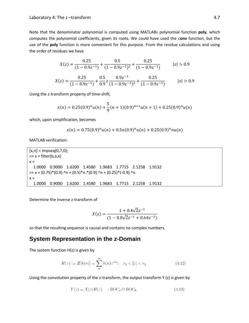
Note that the denominator polynomial is computed using MATLABs polynomial function poly, which

computes the polynomial coefficients, given its roots. We could have used the conv function, but the

use of the poly function is more convenient for this purpose. From the residue calculations and using

the order of residues we have

)

)

)

) | |

)

)

)

) | |

Using the z-transform property of time-shift,

) ) )

) ) ) ) )

which, upon simplification, becomes

) ) ) ) ) ) )

MATLAB verification:

[x,n] = impseq(0,7,0); >> x = filter(b,a,x) x = 1.0000 0.9000 1.6200 1.4580 1.9683 1.7715 2.1258 1.9132 >> x = (0.75)*(0.9).^n + (0.5)*n.*(0.9).^n + (0.25)*(-0.9).^n x = 1.0000 0.9000 1.6200 1.4580 1.9683 1.7715 2.1258 1.9132

Determine the inverse z-transform of

) √

√ )

so that the resulting sequence is causal and contains no complex numbers.

System Representation in the z-Domain

The system function H(z) is given by

Using the convolution property of the z-transform, the output transform Y (z) is given by


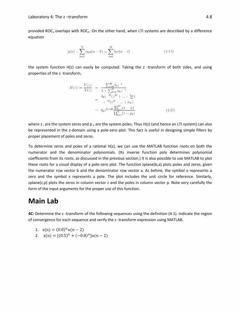
provided ROCx overlaps with ROCh. On the other hand, when LTI systems are described by a difference

equation

the system function H(z) can easily be computed. Taking the z -transform of both sides, and using

properties of the z -transform,

where z l are the system zeros and p k are the system poles. Thus H(z) (and hence an LTI system) can also

be represented in the z-domain using a pole-zero plot. This fact is useful in designing simple filters by

proper placement of poles and zeros.

To determine zeros and poles of a rational H(z), we can use the MATLAB function roots on both the

numerator and the denominator polynomials. (Its inverse function poly determines polynomial

coefficients from its roots, as discussed in the previous section.) It is also possible to use MATLAB to plot

these roots for a visual display of a pole-zero plot. The function zplane(b,a) plots poles and zeros, given

the numerator row vector b and the denominator row vector a. As before, the symbol o represents a

zero and the symbol x represents a pole. The plot includes the unit circle for reference. Similarly,

zplane(z,p) plots the zeros in column vector z and the poles in column vector p. Note very carefully the

form of the input arguments for the proper use of this function.

Main Lab

4C: Determine the z -transform of the following sequences using the definition (4.1). Indicate the region

of convergence for each sequence and verify the z -transform expression using MATLAB.

1. ) ) )

2. ) [ ) ) ] )

laboratory 4: the z –transform

Documents