learning robust features and classiﬁers ... - cse…mchen/papers/criteo2012.pdf · criteo,...

Learning Robust Features and Classifiers through Marginalized CorruptionMinmin Chen

1

Criteo, 2012-12-11

Tuesday, December 11, 12

Outline

2

1. Learning robust features for text data using marginalized Stacked Denoising Autoencoders

2. Learning robust classifiers through marginalized Corrupted Features

3. Learning with reduced labeled data for large scale datasets

4. Learning to generalize across domains

5. Learning with reduced runtime cost for large scale datasets


Outline

3






[M Chen, Z Xu, K Weinberger, F Sha ICML 2012]


Examples of Classifications on Text DataClassify ...

... documentsby topic

... documentsby sentiment


Bag of Words

�

⇧⇧⇧⇧⇧⇧⇧⇤

1020...0

⇥

⌃⌃⌃⌃⌃⌃⌃⌅

sparsebow vector

Kindle

Nookmatch

Ottawa

zulu

Kindle vs. Nook. When I wrote this review in August there was only one Nook ...

input documentdictionary/

Hashing-Trick[Weinberger et al., ICML 2009]


Bag of Words

�

⇧⇧⇧⇧⇧⇧⇧⇤

1020...0

⇥

⌃⌃⌃⌃⌃⌃⌃⌅

sparsebow vector

Kindle

Nookmatch

Ottawa

zulu

linear classifier (SVM)dictionary/

Hashing-Trick[ICML 2009]


What’s Similar?

Last Sunday Manchester United won the game I mentioned.

Recently Obama signed an important bill.

Sunday, our president mentioned a game-changing law.

Which two sentences are most similar?

A:

B:

C:


Cross Domain Feature Incompatibility

8

I read 2-3 books a week, and this is without a doubt my favorite of this year. A beautiful novel by Afghan-American Khaled Hosseini that ranks among the best-written and provocative stories of the year so far.This unusually eloquent story is also about the fragile relationship ….

This unit makes the best coffee I've had in a home. It is my favorite unit. It makes excellent and HOT coffee. The carafe is solidly constructed and fits securely in square body. The timer is easy to program, as is the clock.

target specific

cross domain

source specific(Test Error: 13%)

(Test Error: 24%)


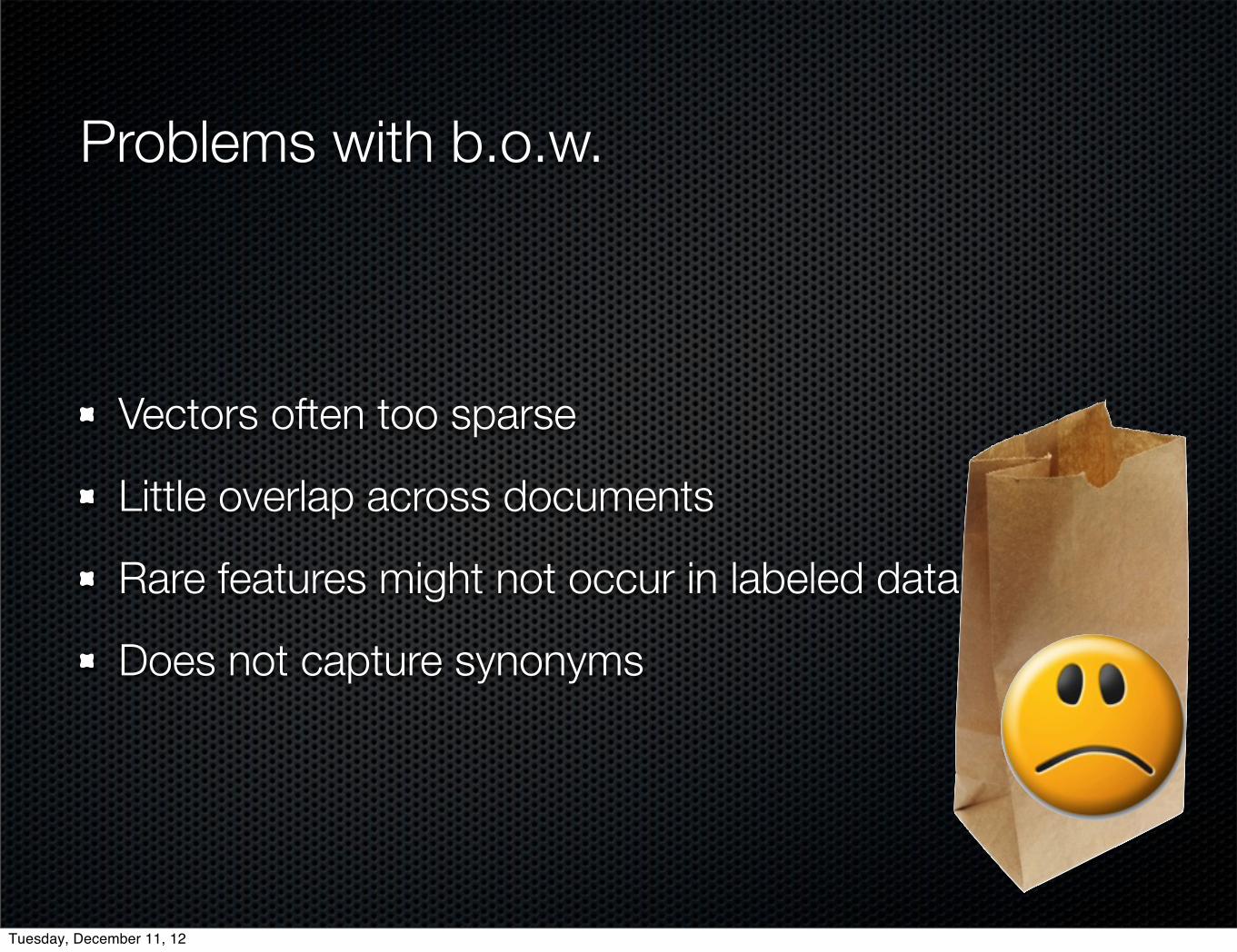
Problems with b.o.w.

Vectors often too sparse

Little overlap across documents

Rare features might not occur in labeled data

Does not capture synonyms


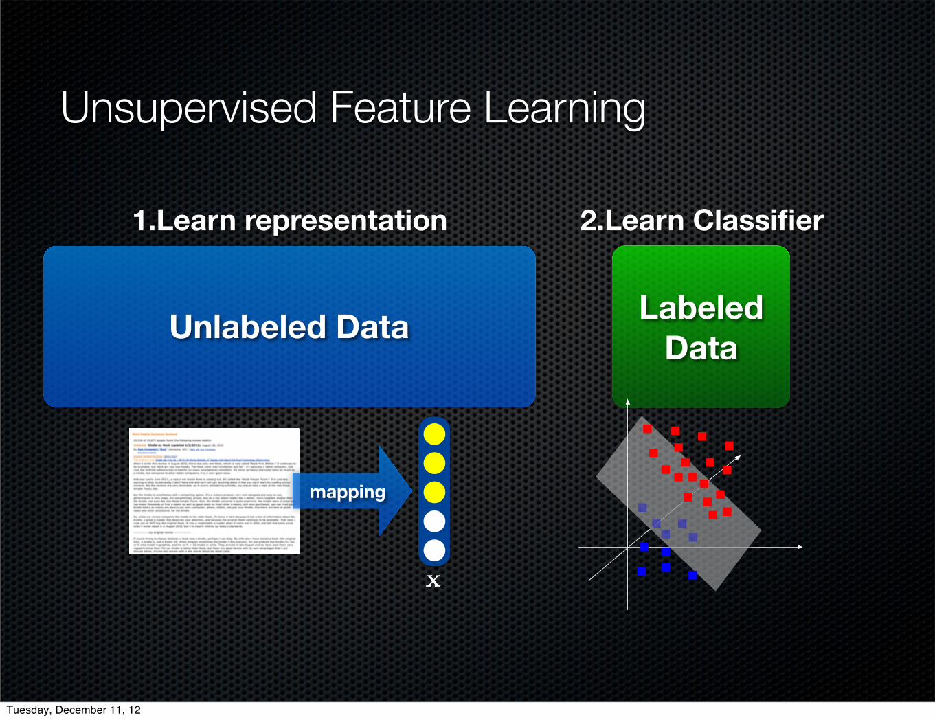
Unsupervised Feature Learning

Unlabeled Data Labeled Data

1.Learn representation 2.Learn Classifier

x

mapping


I read 2-3 books a week, and this is without a doubt my favorite of this year. A beautiful novel by Afghan-American Khaled Hosseini that ranks among the best-written and provocative stories of the


favorite

best-written

energy-efficient

eloquent

solidly-constructed

dictionary

blank-out noise corrupted

x̃

11

clean

x

Denoising Autoencoders (DA)

ydecoder

gW 0(y) fW(x̃)

encoder

A good representation is one that can be obtained robustly from a corrupted input and that will be useful for recovering the corresponding clean input

[Vincent et al., 2008; Glorot et al., 2011]


Accurate but Slow

12

SDAs generate robust features for domain adaptation

Pre-training of SDAs requires (stochastic) gradient descent, slow for large scale dataset

dense-matrix GPU implementation [Bergstra, et al., 2010]

reconstruction sampling [Dauphin et al., 2011]

hyper-parameters (learning rate, number of epochs, noise ratio, mini-batch size, network structure, etc.) [Bergstra and Bengio, 2012]

transfer ratio = error( )

error( )

101 102 103 104 1051

1.1

1.2

1.3

1.4

1.5Bag-of-words (0 secs)

PCA (~3 mins)

SCL (47 secs)

CODA (~25 mins)

SDA (~5 hours)

Training time in seconds (log)

Tran

sfer

Rat

io

faster

bette

r

Cross domain sentiment analysis


13

Keep the accuracyImprove the speed

Research Goal

101 102 103 104 1051

1.1

1.2

1.3

1.4

1.5Bag-of-words (0 secs)

PCA (~3 mins)

SCL (47 secs)

CODA (~25 mins)

SDA (~5 hours)


Tran

sfer

Rat

io

faster

bette

r

holy grail




favorite

best-written

energy-efficient

eloquent

solidly-constructed

dictionary

corrupted

x̃

14

clean

x

marginalized Denoising Autoencoders (mDA)

ydecoder

gW 0(y) fW(x̃)

encoder

A good representation is one that can be obtained robustly from a corrupted input and that will be useful for recovering the corresponding clean input

reconstruction

` =nX

i=1

kxi �Wx̃ik2


SDA vs. mSDA

linear, global minimanon-linear, local minima15Glorot et al. 2010

x

Wx̃

x

x̃ fW gW> z

Chen et al. 2012

` =nX

i=1

kxi �Wx̃ik2`DA =nX

i=1

kxi � g(W>f(Wx̃))k2

Wx̃

significantly speeds up training


any initialization

global minima

16

x̃

reconstruction

x

Closed-form solution

W =

nX

i=1

xix̃>i

! nX

i=1

x̃ix̃>i

!�1

(linear) Denoising Autoencoder

` =nX

i=1

kxi �Wx̃ik2


W =

nX

i=1

xix̃>i

! nX

i=1

x̃ix̃>i

!�1

17

x̃

reconstruction

x


m corruptions for each input

` =nX

i=1

1

m

mX

j=1

kxi �Wx̃i,jk2

W =

0

@nX

i=1

1

m

mX

j=1

xix̃>i,j

1

A

0

@nX

i=1

1

m

mX

j=1

x̃i,j x̃>i,j

1

A�1

x̃1 x̃2 x̃3

m corruptions


x̃m

. . .

(linear) Denoising Autoencoder

` =nX

i=1

kxi �Wx̃ik2


W

⇤ =

nX

i=1

E[xix̃>i ]p(x̃i|xi)

! nX

i=1

E[x̃ix̃>i ]p(x̃i|xi)

!�1

W =

0

@nX

i=1

1

m

mX

j=1

xix̃>i,j

1

A

0

@nX

i=1

1

m

mX

j=1

x̃i,j x̃>i,j

1

A�1

marginalized Denoising Autoencoder(mDA)Marginalized corruption

infinitely many corruptions

18

m ! 1

• closed form!• corruption marginalized out!

x

x̃1 x̃2 x̃3

m corruptions

x̃m

. . .W =

0

@nX

i=1

1

m

mX

j=1

xix̃>i,j

1

A

0

@nX

i=1

1

m

mX

j=1

x̃i,j x̃>i,j

1

A�1

220221222223224225226227228229230231232233234235236237238239240241242243244245246247248249250251252253254255256257258259260261262263264265266267268269270271272273274

275276277278279280281282283284285286287288289290291292293294295296297298299300301302303304305306307308309310311312313314315316317318319320321322323324325326327328329

mSDA for Domain Adaptation

a dense-matrix GPU implementation exist Bergstra et al.(2010)); 2. There are several hyper-parameters (learningrate, number of epochs, noise ratio, mini-batch size andnetwork structure), which need to be set by cross valida-tion — this is particularly expensive as each individual runcan take several hours; 3. The optimization is inherentlynon-convex and initialization dependent, making outcomeseffectively irreproducible.

3. SDA with Marginalized CorruptionIn this section we introduce a modified version of SDA,which preserves its strong feature learning capabilities, butalleviates the concerns mentioned above through speedupsof several orders of magnitudes, fewer meta-parameters,faster model-selection and layer-wise convexity.

3.1. Single-layer Denoiser

The basic building block of our framework is a one-layerdenoising autoencoder. We take the inputs x1, . . . ,xn fromD=DT [DT and corrupt them by random feature removal— each feature is set to 0 with probability p�0. Let usdenote the corrupted version of xi as x̃i. As opposed tothe two-level encoder and decoder in SDA, we reconstructthe corrupted inputs with a single mapping W : Rd!Rd,that minimizes the squared reconstruction loss

1

2n

nX

i=1

kxi �Wx̃ik2. (1)

To simplify notation, we assume that a constant feature isadded to the input, xi = [xi; 1], and an appropriate biasis incorporated within the mapping W = [W,b]. Theconstant feature is never corrupted.

The solution to (1) depends on which features of each inputare randomly corrupted. To lower the variance, we performmultiple passes over the training set, each time with dif-ferent corruption. We solve for the W that minimizes theoverall squared loss

Lsq(W) =1

2mn

mX

j=1

nX

i=1

kxi �Wx̃i,jk2, (2)

where x̃i,j represents the jth corrupted version of the orig-inal input xi.

Let us define the design matrix X = [x1, . . . ,xn] 2Rd⇥n

and its m-times repeated version as X= [X, . . . ,X]. Fur-ther, we denote the corrupted version of X as X̃. With thisnotation, the loss in eq. (1) reduces to

Lsq(W)=1

2nmtr⇣

X�W

eX

⌘> ⇣X�W

eX

⌘�. (3)

Algorithm 1 mDA in MATLABTM.function [W,h]=mDA(X,p);

X=[X;ones(1,size(X,2))];

d=size(X,1);

q=ones(d,1).

*

(1-p); q(end)=1;

S=X

*

X’;

Q=S.

*

(q

*

q’);

Q(1:d+1:end)=q.

*

diag(S);

P=S.

*

repmat(q,1,d);

W=((Q+1e-5

*

eye(d))\P(:,1:end-1))’;

h=W

*

X;

The solution to (3) can be expressed as the well-knownclosed-form solution for ordinary least squares (Bishop,2006):

W = PQ

�1 with Q = eX

eX

> and P = X

eX

>. (4)

(In practice this can be computed as a system of linearequations, without the costly matrix inversion.)

3.2. Marginalized Denoising Autoencoder.

The larger m is, the more corruptions we average over. Ide-ally we would like m ! 1, effectively using infinitelymany copies of noisy data to compute the denoising trans-formation W.

By the weak law of large numbers, the matrices P and Q,as defined in (3), converge to their expected values as mbecomes very large. If we are interested in the limit case,where m!1, we can derive the expectations of Q and P,and express the corresponding mapping W as

W = E[P]E[Q]�1. (5)

In the remainder of this section, we compute the expecta-tions of these two matrices. For now, let us focus on

E[Q] =nX

i=1

E⇥x̃ix̃

>i

⇤. (6)

An off-diagonal entry in the matrix x̃ix̃>i is uncorrupted if

the two features ↵ and � both “survived” the corruption,which happens with probability (1 � p)2. For the diago-nal entries, this holds with probability 1 � p. Let us de-fine a vector q = [1 � p, . . . , 1 � p, 1]> 2 Rd+1, whereq↵ represents the probability of a feature ↵ “surviving” thecorruption. As the constant feature is never corrupted, wehave qd+1=1. If we further define the scatter matrix of theoriginal uncorrupted input as S = XX

>, we can expressthe expectation of the matrix Q as

E[Q]↵,� =

⇢S↵�q↵q� if ↵ 6= �S↵�q↵ if ↵ = �

. (7)

By analogous reasoning, we obtain the expectation of P inclosed-form as E[P]↵� = S↵�q� .

E[xix̃>i ]p(x̃i|xi) E[x̃ix̃

>i ]p(x̃i|xi)


Stacking

h1

input

h01

f h2

hidden

19

favorite

best-written

energy-efficient

eloquent

solidly-constructed

x

hidden

W2 h02 fW

layer 1 layer 2


mSDA for Feature Learning

h1

x

h2

20

new representation linear classifier (SVM)


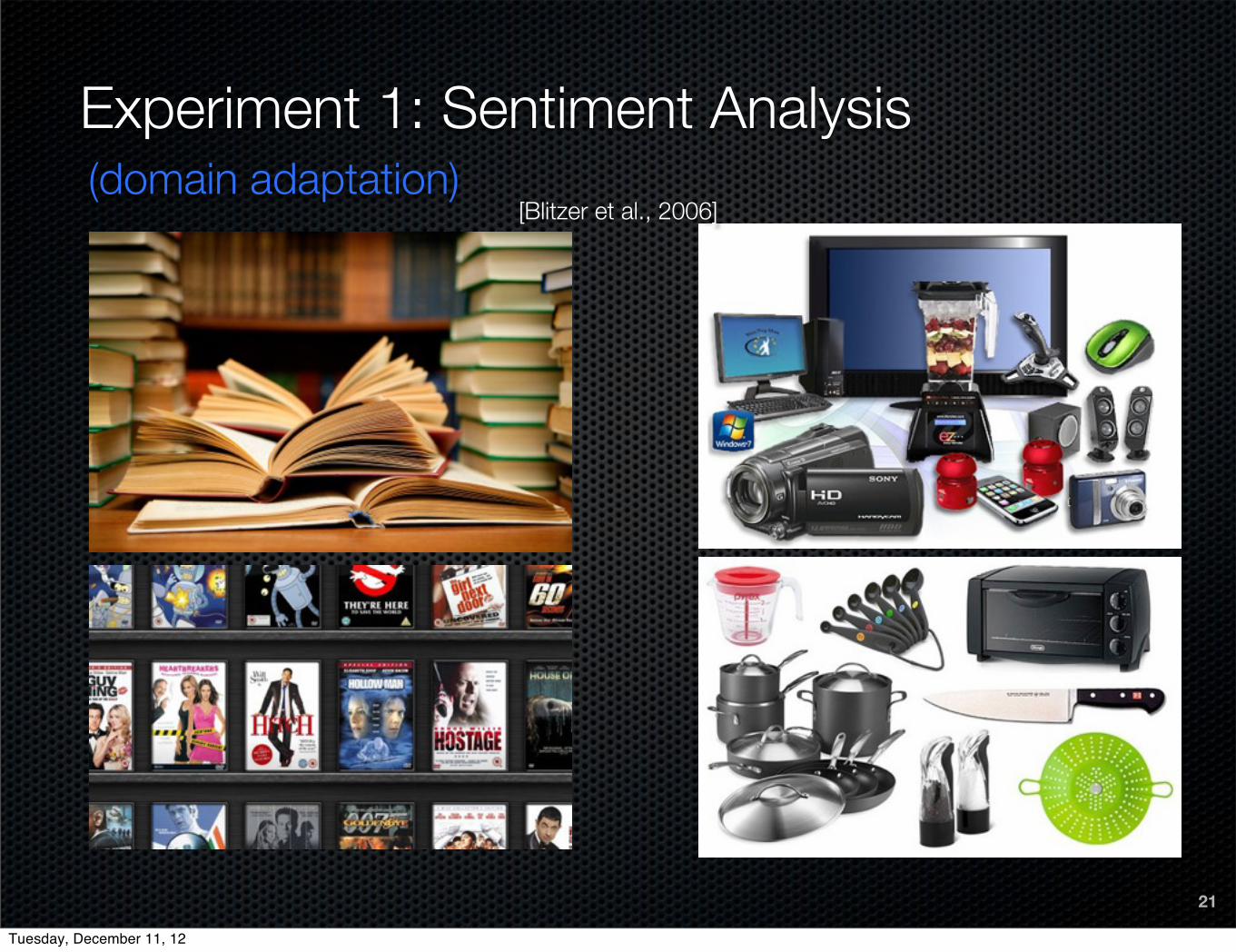
Experiment 1: Sentiment Analysis

21

[Blitzer et al., 2006](domain adaptation)


Unsupervised Feature Learning

Unlabeled Data Labeled Data

1.Learn representation 2.Learn Classifier

x

mapping


Resultsbe

tter

23

transfer loss = error( ) error( )-

4 domains, 12 tasksd = 5,000n = 27,677

D−>B E−>B K−>B B−>D E−>D K−>D B−>E D−>E K−>E B−>K D−>K E−>K−4

−2

0

2

4

6

8

10

12

Tran

sfer

Los

s (%)

D−>B E−>B K−>B B−>D E−>D K−>D B−>E D−>E K−>E B−>K D−>K E−>K−4−2

02468

1012

BaselinePCASCL (Blitzer et. al., 2007)CODA (Chen et. al., 2011)SDA (Glorot et. al., 2011)mSDA (l=5)

new representation b.o.w


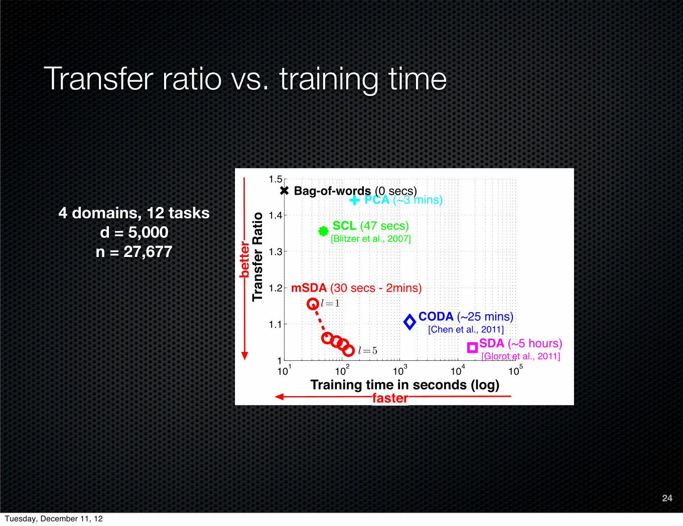
Transfer ratio vs. training time

24

4 domains, 12 tasksd = 5,000n = 27,677

101 102 103 104 1051

1.1

1.2

1.3

1.4

1.5

faster

bette

r


Tran

sfer

Rat

io

PCA (~3 mins)

l=1

l=5

mSDA (30 secs - 2mins)

Bag-of-words (0 secs)

SCL (47 secs)[Blitzer et al., 2007]

CODA (~25 mins)[Chen et al., 2011]

SDA (~5 hours)[Glorot et al., 2011]


Large data set

25

20 domains, 380 tasksd = 5,000

n = 339,675

101 102 103 104 105 1061

1.05

1.1

1.15

1.2

1.25

1.3

1.35

faster

bette

r


Tran

sfer

Rat

io

SDA (~2 days 8 hours)[Glorot et al., 2011]

mSDA (6 mins - 23 mins)


l=1

l=5


26

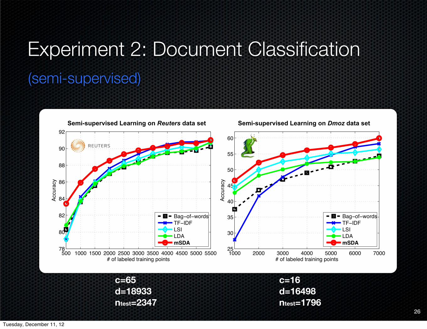
Experiment 2: Document Classification

c=65d=18933ntest=2347

c=16d=16498ntest=1796

(semi-supervised)

Semi-supervised Learning on Reuters data set Semi-supervised Learning on Dmoz data set

1000 2000 3000 4000 5000 6000 700025

30

35

40

45

50

55

60

# of labeled training points

Accu

racy

Bag−of−wordsTF−IDFLSILDAmSDA

500 1000 1500 2000 2500 3000 3500 4000 4500 5000 550078

80

82

84

86

88

90

92

# of labeled training points

Accu

racy

Bag−of−wordsTF−IDFLSILDAmSDA


Learning the hidden topics

27

reaganreagonhouse

administrationwhite

presidentcongresssenate

billstatesunited

bushpresidentgeorgereaganhousewhite

secretaryvice

politicalchief

senate

unionunionsoviet

workersstrike

contractunited

employeeswage

membersmoscow

“ ”year

billiondlrsmin

sharemarketbank

interestpricedebt

nasdaqnasdaqnational

nasdsystem

exchangeassociation

stocksecuritiestradingcomon

reproductioncropareas

weathercorndry

moisturenormalgood

agriculturewinter

Reuters newswire 1987


marginalized Stacked Denoising Autoencoder (mSDA)

marginalizes out corruption

keeps high accuracy of SDAs but is orders of magnitudes faster

Optimization:

is layer-wise convex

has layer-wise closed form solutions

is easy to implement

Conclusion

28





Optimization:




Conclusion

29

marginalize out


101 102 103 104 1051

1.1

1.2

1.3

1.4

1.5

faster

bette

r


Tran

sfer

Rat

io

PCA (~3 mins)

SCL (47 secs)

CODA (~25 mins)

SDA (~5 hours)

l=1

l=5

mSDA (30 secs - 2mins)


Conclusion

30




Optimization:





Conclusion

31




Optimization:





Conclusion

32




Optimization:








Optimization:




Conclusion

33


struct, and be reconstructed by, co-occurring features, typ-ically of similar sentiment (e.g. “good” or “love”). Hence,the source-trained classifier can assign weights even to fea-tures that never occur in its original domain representation,which are “re-constructed” by the SDA.

Although SDAs generate excellent features for domainadaptation, they have several drawbacks: 1. Training with(stochastic) gradient descent is slow and hard to paral-lelize (although a dense-matrix GPU implementation ex-ists (Bergstra et al., 2010) and an implementation basedon reconstruction sampling exists (Dauphin Y., 2011) forsparse inputs); 2. There are several hyper-parameters(learning rate, number of epochs, noise ratio, mini-batchsize and network structure), which need to be set by crossvalidation — this is particularly expensive as each individ-ual run can take several hours; 3. The optimization is in-herently non-convex and dependent on its initialization.

3. SDA with Marginalized CorruptionIn this section we introduce a modified version of SDA,which preserves its strong feature learning capabilities, andalleviates the concerns mentioned above through speedupsof several orders of magnitudes, fewer meta-parameters,faster model-selection and layer-wise convexity.

3.1. Single-layer Denoiser

The basic building block of our framework is a one-layerdenoising autoencoder. We take the inputs x1, . . . ,xn fromD=DS[DT and corrupt them by random feature removal— each feature is set to 0 with probability p�0. Let usdenote the corrupted version of xi as x̃i. As opposed tothe two-level encoder and decoder in SDA, we reconstructthe corrupted inputs with a single mapping W : Rd!Rd,that minimizes the squared reconstruction loss

1

2n

nX

i=1

kxi �Wx̃ik2. (1)

To simplify notation, we assume that a constant feature isadded to the input, xi = [xi; 1], and an appropriate biasis incorporated within the mapping W = [W,b]. Theconstant feature is never corrupted.

The solution to (1) depends on which features of each inputare randomly corrupted. To lower the variance, we performmultiple passes over the training set, each time with dif-ferent corruption. We solve for the W that minimizes theoverall squared loss

Lsq(W) =1

2mn

mX

j=1

nX

i=1

kxi �Wx̃i,jk2, (2)

where x̃i,j represents the jth corrupted version of the orig-inal input xi.

Algorithm 1 mDA in MATLABTM.function [W,h]=mDA(X,p);

X=[X;ones(1,size(X,2))];

d=size(X,1);

q=[ones(d-1,1).

*

(1-p); 1];

S=X

*

X’;

Q=S.

*

(q

*

q’);

Q(1:d+1:end)=q.

*

diag(S);

P=S.

*

repmat(q’,d,1);

W=P(1:end-1,:)/(Q+1e-5

*

eye(d));

h=tanh(W

*

X);

Let us define the design matrix X = [x1, . . . ,xn] 2Rd⇥n

and its m-times repeated version as X= [X, . . . ,X]. Fur-ther, we denote the corrupted version of X as X̃. With thisnotation, the loss in eq. (1) reduces to

Lsq(W)=1

2nmtr⇣

X�W

eX

⌘> ⇣X�W

eX

⌘�. (3)

The solution to (3) can be expressed as the well-knownclosed-form solution for ordinary least squares (Bishop,2006):

W = PQ

�1 with Q = eX

eX

> and P = X

eX

>. (4)

(In practice this can be computed as a system of linearequations, without the costly matrix inversion.)

3.2. Marginalized Denoising Autoencoder

The larger m is, the more corruptions we average over. Ide-ally we would like m ! 1, effectively using infinitelymany copies of noisy data to compute the denoising trans-formation W.

By the weak law of large numbers, the matrices P and Q,as defined in (3), converge to their expected values as mbecomes very large. If we are interested in the limit case,where m!1, we can derive the expectations of Q and P,and express the corresponding mapping W as

W = E[P]E[Q]�1. (5)

In the remainder of this section, we compute the expecta-tions of these two matrices. For now, let us focus on

E[Q] =nX

i=1

E⇥x̃ix̃

>i

⇤. (6)

An off-diagonal entry in the matrix x̃ix̃>i is uncorrupted if

the two features ↵ and � both “survived” the corruption,which happens with probability (1 � p)2. For the diago-nal entries, this holds with probability 1 � p. Let us de-fine a vector q = [1 � p, . . . , 1 � p, 1]> 2 Rd+1, whereq↵ represents the probability of a feature ↵ “surviving” thecorruption. As the constant feature is never corrupted, we


have qd+1=1. If we further define the scatter matrix of theoriginal uncorrupted input as S = XX

>, we can expressthe expectation of the matrix Q as

E[Q]↵,� =

⇢S↵�q↵q� if ↵ 6= �S↵�q↵ if ↵ = �

. (7)

Similarly, we obtain the expectation of P in closed-form asE[P]↵� = S↵�q� .

With the help of these expected matrices, we can com-pute the reconstructive mapping W directly in closed-formwithout ever explicitly constructing a single corrupted in-put x̃i. We refer to this algorithm as marginalized De-noising Autoencoder (mDA). Algorithm 1 shows a 10-lineMATLABTM implementation. The mDA has several ad-vantages over traditional denoisers: 1. It requires onlya single sweep through the data to compute the matricesE[Q], E[P]; 2. Training is convex and a globally optimalsolution is guaranteed; 3. The optimization is performed innon-iterative closed-form.

3.3. Nonlinear feature generation and stacking

Arguably two of the key contributors to the success of theSDA are its nonlinearity and the stacking of multiple lay-ers of denoising autoencoders to create a “deep” learningarchitecture. Our framework has the same capabilities.

In SDAs, the nonlinearity is injected through the nonlin-ear encoder function h(·), which is learned together withthe reconstruction weights W. Such an approach makesthe training procedure highly non-convex and requires it-erative procedures to learn the model parameters. To pre-serve the closed-form solution from the linear mapping insection 3.2 we insert nonlinearity into our learned repre-sentation after the weights W are computed. A nonlinearsquashing-function is applied on the output of each mDA.Several choices are possible, including sigmoid, hyperbolictangent, tanh(), or the rectifier function (Nair & Hinton,2010). Throughout this work, we use the tanh() function.

Inspired by the layer-wise stacking of SDA, we stack sev-eral mDA layers by feeding the output of the (t�1)th mDA(after the squashing function) as the input into the tth mDA.Let us denote the output of the tth mDA as ht and the orig-inal input as h

0 = x. The training is performed greedilylayer by layer: each map W

t is learned (in closed-form)to reconstruct the previous mDA output ht�1 from all pos-sible corruptions and the output of the tth layer becomesh

t = tanh(Wth

t�1). In our experiments, we found thateven without the nonlinear squashing function, stackingstill improves the performance. However, the nonlinearityimproves over the linear stacking significantly. We refer tothe stacked denoising algorithm as marginalized StackedDenoising Autoencoder (mSDA). Algorithm 2 shows a 8-lines MATLABTM implementation of mSDA.

Algorithm 2 mSDA in MATLABTM.function [Ws,hs]=mSDA(X,p,l);

[d,n]=size(X);

Ws=zeros(d,d+1,l);

hs=zeros(d,n,l+1);

hs(:,:,1)=X;

for t=1:l

[Ws(:,:,t), hs(:,:,t+1)]=mDA(hs(:,:,t),p);

end;

3.4. mSDA for Domain Adaptation

We apply mSDA to domain adaptation by first learning fea-tures in an unsupervised fashion on the union of the sourceand target data sets. One observation reported in (Glo-rot et al., 2011) is that if multiple domains are available,sharing the unsupervised pre-training of SDA across all do-mains is beneficial compared to pre-training on the sourceand target only. We observe a similar trend with our ap-proach. The results reported in section 5 are based on fea-tures learned on data from all available domains. Once amSDA is trained, the output of all layers, after squashing,tanh(Wt

h

t�1), combined with the original features h

0,are concatenated and form the new representation. All in-puts are transformed into the new feature space. A linearSupport Vector Machine (SVM) (Chang & Lin, 2011) isthen trained on the transformed source inputs and testedon the target domain. There are two meta-parameters inmSDA: the corruption probability p and the number of lay-ers l. In our experiments, both are set with 5-fold crossvalidation on the labeled data from the source domain. Asthe mSDA training is almost instantaneous, this grid searchis almost entirely dominated by the SVM training time.

4. Extension for High Dimensional DataMany data sets (e.g. bag-of-words text documents) are nat-urally high dimensional. As the dimensionality increases,hill-climbing approaches used in SDAs can become pro-hibitively expensive. In practice, a work-around is to trun-cate the input data to the r⌧d most common features (Glo-rot et al., 2011). Unfortunately, this prevents SDAs fromutilizing important information found in rarer features. (Aswe show in section 5, including these rarer features leadsto significantly better results.) High dimensionality alsoposes a challenge to mSDA, as the system of linear equa-tions in (5) of complexity O(d3) becomes too costly. Inthis section we describe how to approximate this calcula-tion with a simple division into d

r sub-problems of O(r3).

We combine the concept of “pivot features” from Blitzeret al. (2006) and the use of most-frequent featuresfrom Glorot et al. (2011). Instead of learning a single map-ping W 2 Rd⇥(d+1) to reconstruct all corrupted features,we learn multiple mappings but only reconstruct the r⌧d


Outline

34






[M Chen, Z Xu, K Weinberger, F Sha ICML 2012]


Outline

35






[L Maaten, M Chen, S Tyree, K Weinberger, ICML 2013]


Empirical Risk Minimization

36

Ideally, we learn our predictor on infinite training data

In practice, we learn our predictor on finite training data

−10 −8 −6 −4 −2 0 2 4 6 8 100

0.02

0.04

0.06

0.08

0.1

0.12

0.14

0.16

−10 −8 −6 −4 −2 0 2 4 6 8 100

0.02

0.04

0.06

0.08

0.1

0.12

0.14

0.16

min⇥

L(D;⇥) =nX

i=1

`(xi, yi;⇥)


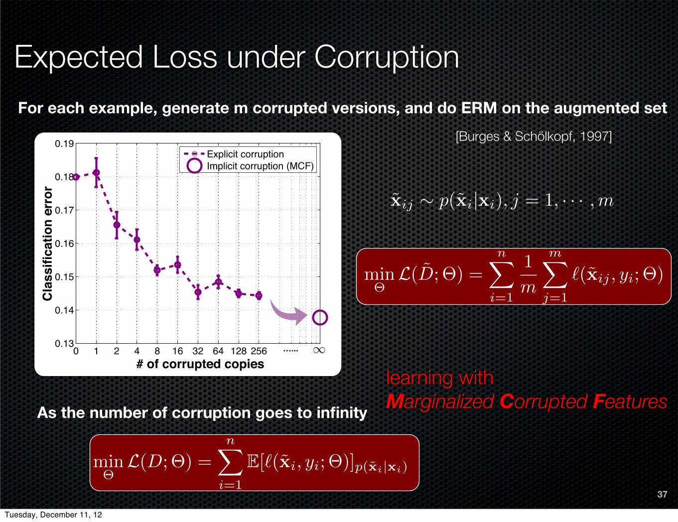
Expected Loss under Corruption

37

0 1 2 4 8 16 32 64 128 256 inf0.13

0.14

0.15

0.16

0.17

0.18

0.19

Noise

Erro

r

Explicit corruptionImplicit corruption (MCF)

# of corrupted copies

Cla

ssifi

catio

n er

ror

…... 11

For each example, generate m corrupted versions, and do ERM on the augmented set

As the number of corruption goes to infinity

min⇥

L(D;⇥) =nX

i=1

E[`(x̃i, yi;⇥)]p(x̃i|xi)

x̃ij ⇠ p(x̃i|xi), j = 1, · · · ,m

min⇥

L(D̃;⇥) =nX

i=1

1

m

mX

j=1

`(x̃ij , yi;⇥)

[Burges & Schölkopf, 1997]

learning withMarginalized Corrupted Features


Quadratic LossWe can derive plug-in solutions for the quadratic, exponential and logistic functions for a range of corrupting distributions

We can derive the optimal solution under closed form as long as the mean and variance of the corrupting distribution can be computed analytically.

infinite copies, same computation

minw

L(D;w) =nX

i=1

E[(w>x̃i � yi)

2]p(x̃i|xi)

= w

>

nX

i=1

E[x̃i]E[x̃i]> + V[x̃i]

!w � 2

nX

i=1

yiE[x̃i]

!>

w + const

w

⇤ =

nX

i=1

E[x̃i]E[x̃i]> + V[x̃i]

!�1 nX

i=1

yiE[x̃i]

!

0 1 2 4 8 16 32 64 128 256 inf0.13

0.14

0.15

0.16

0.17

0.18

0.19

Noise

Erro

r



Cla

ssifi

catio

n er

ror

…... 11


Corrupting Distributions of Interest

39

220221222223224225226227228229230231232233234235236237238239240241242243244245246247248249250251252253254255256257258259260261262263264265266267268269270271272273274

275276277278279280281282283284285286287288289290291292293294295296297298299300301302303304305306307308309310311312313314315316317318319320321322323324325326327328329

Learning with Marginalized Corrupted Features

Distribution PDF E[x̃nd

]

p(x̃nd|xnd)V [x̃

nd

]

p(x̃nd|xnd)

Blankout noisep(x̃

nd

= 0) = q

d

p(x̃nd

= x

nd

) = 1�q

d

(1 � q

d

)xnd

q

d

(1 � q

d

)x2nd

Bit-swap noisep(x̃

nd

= 1�x

nd

) = q

d

p(x̃nd

= x

nd

) = 1�q

d

q

(1�xnd)d

(1 � q

d

)xnd (1 � b) b, b=q

(1�xnd)d

(1 � q

d

)xnd

Gaussian noise p(x̃nd

|x

nd

) = N (x̃nd

|x

nd

,�

2) x

nd

�

2

Laplace noise p(x̃nd

|x

nd

) = Lap(x̃nd

|x

nd

,�) x

nd

2�2

Poisson noise p(x̃nd

|x

nd

) = Pois(x̃nd

|x

nd

) x

nd

x

nd

Table 1. The probability density function (PDF), mean, and variance of corrupting distributions of interest. Thesequantities can be plugged into equation (3) to obtain the expected value under the corrupting distribution of the quadratic.

predictors that we refer to as learning with marginal-

ized corrupted features (MCF).

3.1. Specific loss functions

The tractability of (2) depends on the choice of lossfunction and corrupting distribution P

E

. In this sec-tion, we show that for linear predictors that employa quadratic or exponential loss function, the requiredexpectations under p(x̃|x) in (2) can be computed an-alytically for all corrupting distributions in the naturalexponential family. For linear predictors with logisticloss, we derive an upper bound on the expected valueof the loss under p(x̃|x).

Quadratic loss. Assuming a label variable y 2

{�1,+1}, the expected value of the quadratic loss un-der corrupting distribution p(x̃|x) is given by:

L(D;w) =NX

n=1

E"✓

w

Tx̃

n

� y

n

◆2#

p(x̃n|xn)

= w

T

✓NX

n=1

E[x̃n

]E[x̃n

]T + V [x̃n

]

◆w

� 2

✓NX

n=1

y

n

E [x̃n

]

◆T

w +N, (3)

wihere V [x] denotes the variance of x, and all expec-tations are under p(x̃

n

|x

n

). The expected quadraticloss is convex irrespective of what corruption model isused; the optimal solution w

⇤ is given by:

w

⇤ =

✓NX

n=1

E[x̃n

]E[x̃n

]T + V [x̃n

]

◆�1✓ NX

n=1

y

n

E [x̃n

]

◆.

To minimize the expected quadratic loss under the cor-ruption model, we only need to compute the mean andvariance of the corrupting distribution, which is prac-tical for all exponential-family distributions. Table 1gives an overview of these quantities for some corrupt-ing distributions of interest.

An interesting special case of MCF with quadratic lossoccurs when p(x̃|x) is the isotropic Gaussian distribu-tion with mean x and variance �

2I. For such a noise

model, we obtain as special case (Chapelle et al., 2000):

L(D;w) = w

T

✓NX

n=1

x

n

x

Tn

◆w

� 2

✓NX

n=1

y

n

x

n

◆T

w + �

2Nw

Tw +N,

which is the standard l2-regularized quadratic losswith regularization parameter �2

N . Interestingly, us-ing MCF with Laplace noise also leads to ridge regres-sion (with regularization parameter 2�2

N).

Exponential loss. The expected value of the expo-nential loss under corruption model p(x̃|x) is:

L(D;w) =NX

n=1

Ehe

�ynwTx̃n

i

p(x̃n|xn)

=NX

n=1

DY

d=1

E⇥e

�ynwdx̃nd⇤p(x̃nd|xnd)

, (4)

which can be recognized as a product of moment-generating functions E[exp(t

nd

x̃

nd

)] with t

nd

=�y

n

w

d

.By definition, the moment-generating function (MGF)can be computed for all corrupting distributions inthe natural exponential family. An overview of themoment-generating functions for some corrupting dis-tributions of interest is given in Table 2. The expectedexponential loss is convex whenever the MGF is log-linear in w

d

(e.g., for blankout or Gaussian noise).

The derivation above can readily be extended to multi-class exponential loss (Zhu et al., 2006) by replacingthe weight vector w by a D⇥K weight matrix W,and by replacing the labels y by label vectors y ={1,� 1

K�1}

K withP

K

k=1 yk = 0.

Logistic loss. In the case of the logistic loss, thesolution to (2) cannot be computed in closed form.

Similar conclusion can be reached for exponential loss (using moment generating function of exponential family distributions), and logistic loss (using Jensen’s inequality)

Gaussian corruption leads to an interesting special case:

L(D;w) = w

>

nX

i=1

xix>i

!w � 2

nX

i=1

yixi

!>

w + n�

2w

>w + const


40

Blankout corruption Poisson corruption550551552553554555556557558559560561562563564565566567568569570571572573574575576577578579580581582583584585586587588589590591592593594595596597598599600601602603604

605606607608609610611612613614615616617618619620621622623624625626627628629630631632633634635636637638639640641642643644645646647648649650651652653654655656657658659


0 1 2 4 8 16 32 64 128 256 inf0.13

0.14

0.15

0.16

0.17

0.18

0.19

Noise

Erro

r



Cla

ssifi

catio

n er

ror

…...11

Figure 2. Comparison between MCF and explicitly addingcorrupted examples to the training set (for quadratic loss)on the Amazon (books) data using blankout corruption.Training with MCF is equivalent to using infinitely manycorrupted copies of the training data.

Figure 3 presents the results of a second set of ex-periments on Dmoz and Reuters, in which we studyhow the performance of MCF depends on the amountof training data. For each training set size, we re-peat the experiment five times with randomly sub-sampled training sets; the figure reports the meantest errors and the corresponding standard deviations.The results show that classifiers trained with MCF(solid curves) significantly outperform their counter-parts without MCF (dashed curves). The performanceimprovement is consistent irrespective of the trainingset size, viz. up to 25% on the Dmoz data set.

Explicit vs. implicit feature corruption. Fig-ure 2 shows the classification error on Amazon (books)when a classifier without MCF is trained on the dataset with additional explicitly corrupted samples, as for-mulated in (3). Specifically, we use the blankout cor-ruption model with q set by cross-validation for eachsetting, and we train the classifiers with quadratic lossand l2-regularization. The graph shows a clear trendthat the error decreases when the training set con-tains more corrupted versions of the original trainingdata, i.e. with higher M in eq. (3). The graph il-lustrates that the best performance is obtained as M

approaches infinity, which is equivalent to MCF withblankout corruption (big marker in the bottom right,with q=0.9).

4.2. Image classification

We perform image-classification experiments withMCF on the CIFAR-10 data set (Krizhevsky, 2009),which is a subset of the 80 million tiny images (Tor-ralba et al., 2008). The data set contains RGB imageswith 10 classes of size 32⇥32, and consists of a fixed

# of labeled training data

Blankout / DMOZ

Poisson / DMOZ

Blankout / Reuters

Poisson / Reuters

100 200 400 800 1600 3200 7184

0.4

0.5

0.6

0.7

0.8

Exponential loss (L2)Logistic loss (L2)Quadratic loss (L2)Blankout MCF (exp.)Blankout MCF (log.)Blankout MCF (qua.)

100 200 400 800 1600 3200 5946

0.1

0.15

0.2

0.25

0.3

100 200 400 800 1600 3200 7184

0.4

0.5

0.6

0.7

0.8

Exponential loss (L2)Logistic loss (L2)Quadratic loss (L2)Poisson MCF (exp.)Poisson MCF (log.)Poisson MCF (qua.)

100 200 400 800 1600 3200 5946

0.1

0.15

0.2

0.25

0.3

Clas

sific

atio

n er

ror

Figure 3. The performance of standard and MCF classi-fiers with blankout and Poisson corruption models as afunction of training set size on the Dmoz and Reuters datasets. Both the standard and MCF predictors employ l2-regularization. Figure best viewed in color.

550551552553554555556557558559560561562563564565566567568569570571572573574575576577578579580581582583584585586587588589590591592593594595596597598599600601602603604

605606607608609610611612613614615616617618619620621622623624625626627628629630631632633634635636637638639640641642643644645646647648649650651652653654655656657658659


0 1 2 4 8 16 32 64 128 256 inf0.13

0.14

0.15

0.16

0.17

0.18

0.19

NoiseEr

ror


# of corrupted copiesC

lass

ifica

tion

erro

r…...

11

Figure 2. Comparison between MCF and explicitly addingcorrupted examples to the training set (for quadratic loss)on the Amazon (books) data using blankout corruption.Training with MCF is equivalent to using infinitely manycorrupted copies of the training data.

Figure 3 presents the results of a second set of ex-periments on Dmoz and Reuters, in which we studyhow the performance of MCF depends on the amountof training data. For each training set size, we re-peat the experiment five times with randomly sub-sampled training sets; the figure reports the meantest errors and the corresponding standard deviations.The results show that classifiers trained with MCF(solid curves) significantly outperform their counter-parts without MCF (dashed curves). The performanceimprovement is consistent irrespective of the trainingset size, viz. up to 25% on the Dmoz data set.

Explicit vs. implicit feature corruption. Fig-ure 2 shows the classification error on Amazon (books)when a classifier without MCF is trained on the dataset with additional explicitly corrupted samples, as for-mulated in (3). Specifically, we use the blankout cor-ruption model with q set by cross-validation for eachsetting, and we train the classifiers with quadratic lossand l2-regularization. The graph shows a clear trendthat the error decreases when the training set con-tains more corrupted versions of the original trainingdata, i.e. with higher M in eq. (3). The graph il-lustrates that the best performance is obtained as M

approaches infinity, which is equivalent to MCF withblankout corruption (big marker in the bottom right,with q=0.9).


We perform image-classification experiments withMCF on the CIFAR-10 data set (Krizhevsky, 2009),which is a subset of the 80 million tiny images (Tor-ralba et al., 2008). The data set contains RGB imageswith 10 classes of size 32⇥32, and consists of a fixed


Blankout / DMOZ

Poisson / DMOZ

Blankout / Reuters

Poisson / Reuters

100 200 400 800 1600 3200 7184

0.4

0.5

0.6

0.7

0.8

Exponential loss (L2)Logistic loss (L2)Quadratic loss (L2)Blankout MCF (exp.)Blankout MCF (log.)Blankout MCF (qua.)

100 200 400 800 1600 3200 5946

0.1

0.15

0.2

0.25

0.3

100 200 400 800 1600 3200 7184

0.4

0.5

0.6

0.7

0.8

Exponential loss (L2)Logistic loss (L2)Quadratic loss (L2)Poisson MCF (exp.)Poisson MCF (log.)Poisson MCF (qua.)

100 200 400 800 1600 3200 5946

0.1

0.15

0.2

0.25

0.3

Clas

sific

atio

n er

ror

Figure 3. The performance of standard and MCF classi-fiers with blankout and Poisson corruption models as afunction of training set size on the Dmoz and Reuters datasets. Both the standard and MCF predictors employ l2-regularization. Figure best viewed in color.

Experiment 1: Text Classification Dmoz dataset

c=16d=16498ntest=1796


41

Experiment 2: Image Classification 550551552553554555556557558559560561562563564565566567568569570571572573574575576577578579580581582583584585586587588589590591592593594595596597598599600601602603604

605606607608609610611612613614615616617618619620621622623624625626627628629630631632633634635636637638639640641642643644645646647648649650651652653654655656657658659


100 200 400 800 1600 3200 64000.05

0.1

0.15

0.2

0.25

0.3

0.35reuters


Erro

r

Quadratic loss (L2)Exponential loss (L2)MCF quadratic lossMCF exponential loss

100 200 400 800 1600 3200 64000.3

0.4

0.5

0.6

0.7

0.8

0.9dmoz


Erro

r

Quadratic loss (L2)Exponential loss (L2)MCF quadratic lossMCF exponential loss

# of labeled training data # of labeled training data

Dmoz Reuters

Cla

ssifi

catio

n er

ror

Figure 2. The performance of standard and MCF classifiers with blankoutand Poisson corruption models as a function of the amount labeled trainingdata on the Dmoz and Reuters data sets. Both the standard and MCFpredictors employ l2-regularization. Figure best viewed in color.

0 1 2 4 8 16 32 64 128 256 inf0.13

0.14

0.15

0.16

0.17

0.18

0.19

NoiseEr

ror


# of corrupted copiesC

lass

ifica

tion

erro

r…...

11

Figure 3. Comparison between MCFand explicitly adding corrupted exam-ples to the training set (for quadraticloss) on the Amazon (books) data – us-ing a blankout corruption model withq=??.

Explicit vs. implicit feature corruption. Figure 3shows the classification error on Amazon (books) whena classifier without MCF is trained on the data set withadditional explicitly corrupted samples, as formulatedin (3). Specifically, we use the blankout corruptionmodel with q=??, and we trained the classifiers withquadratic loss and l2-regularization. The graph showsa clear trend that the error decreases when the trainingset contains more corrupted versions of the originaltraining data, i.e. with higherM in eq. (3). The graphillustrates that the best performance is obtained as Mapproaches infinity, which is equivalent to MCF withblankout corruption (big marker in the bottom right).


We perform image-classification experiments withMCF on the CIFAR-10 data set (Krizhevsky, 2009),which is a subset of the 80 million tiny images (Tor-ralba et al., 2008). The data set contains RGB imageswith 10 classes of size 32⇥ 32, and contains 50, 000training and 10, 000 test images.

Setup. We followed the experimental setup of Coateset al. (2011): we whiten the images, extract a set of 7⇥7image patches from the training images, and constructa codebook by running k-means clustering on these im-age patches (with k = 2, 048). Next, we slide a 7⇥7pixel window over the image and identify the nearestprototype in the codebook for each window location.We construct a descriptor2 for each image by subdi-viding it into four equally sized quadrants and count-

2This way of extracting the image features is referred toby Coates et al. (2011) as k-means with hard assignment,average pooling, patch size 7⇥7, and stride 1.

Quadr. Expon. Logist.

No MCF 32.6% 39.7% 38.0%Poisson MCF 29.1% 39.5% 30.0%Blankout MCF 32.3% 37.9% 29.4%

Table 3. Classification errors obtained on the CIFAR-10data set with MCF classifiers trained on simple spatial-pyramid bag-of-visual-words features (lower is better).

ing the number of times each prototype occurs in eachquadrant. This leads to a descriptor of dimensional-ity D = 4⇥2, 048. Because all images have the samesize, we did not normalize the descriptors. We trainedMCF predictors with blankout and Poisson corruptionon the full set of training images, cross-validating overa range of l2-regularization parameters. Subsequently,we measure the classification error of the final predic-tors on the test set.

Results. The results are reported in Table 3. Thebaseline classifiers (without MCF) are on par with the68.8% accuracy reported by Coates et al. (2011) withexactly the same experimental setup. The results il-lustrate the potential of MCF classifiers to improvethe prediction performance on bag-of-visual-words fea-tures, in particular, when using quadratic loss and aPoisson corruption model. (Again, note that Poissoncorruption introduces no additional hyperparametersthat need to be optimized.)

Although our focus in this section is to merely il-lustrate the potential of MCF on image classificationtasks, it is worth noting that the best results in Table 3match those of a highly non-linear mean-covarianceRBMs trained on the same data (Ranzato & Hinton,

CIFAR-10 dataset10 classes50K images4x2048 features

Despite our use of very simple features and predictors, our results are on par with various very sophis t icated deep learners (Coates et al., 2011)


42

Experiment 3: Nightmare at Test Time

0% 10% 20% 30% 40% 50% 60% 70% 80% 90%

0.1

0.2

0.3

0.4

0.5

Percentage of deletions

Clas

sific

atio

n er

ror

Quadratic loss (L2)Exponential loss (L2)Logistic loss (L2)Hinge loss (L2)Hinge loss (FDROP)MCF quadratic lossMCF exponential lossMCF logistic loss

Some features are randomly removed during test (e.g., due to sensor failure or the computation of features exceed certain budget)




derives plug-in solutions for a wide range of loss functions and corrupting distribution

improves the generalization of classifiers without increasing computation

Conclusion

43


Outline

44







Outline

45






[M Chen, K Weinberger, Y Chen ICML 2011]


Challenges: hundreds of thousands of categories

46

As data size scales up, the number of categories also grows

50 labeled per class ＝ 1 million instances

65,348 categories

21,841 categories

1,015,171 categories


What if your classifier could search the web - and use the results to improve its accuracy ?

47

Solution: learning from the web

Motivation and backgroundPseudo Multi-view Co-training

Experimental ResultConclusion

MotivationCo-training and its limitation

Caltech-256 Object Recognition

Americanflag BasketballhoopHotairballoon

?AK47

Frog k

?Frog Cake

BeermugEiffeltower Hawksbill

Problem : manual labeling is expensive!

Minmin Chen, Kilian Weinberger, Yixin Chen Pseudo Multi-view Co-training 3

Airplane

Caltech-256 object recognition task


Results

48

Our contribution: 1. create labeled data automatically2. train classifier during data labeling3. generalize co-training to single view data

Automatic Feature Decomposition for Co-training

5 10 15 20 25 30 35 40 45 5015

20

25

30

35

40

Number of target training images

Accu

racy

(%)

Caltech256 with weakly labeled web images

PMCLRt

LRt F s

RFSSVMt (Bergamo,NIPS2010)DWSVM (Bergamo,NIPS2010)TSVM (Bergamo,NIPS2010)

Figure 4. Recognition accuracy obtained with 300 web im-ages and a varying number of Caltech256 training examplesm.

selected the highest ranked negative and lowest rankedpositive images. The figure showcases how PMC e↵ec-tively identifies relevant images that are similar in styleto the training set for rote-learning. Also, it showcasesthat PMC can potentially be used for image re-rankingof search engines, which is particularly visible in themiddle row where it ignores completely irrelevant im-ages to the category “Ei↵el Tower”, which are rankedsecond to fourth on BingTM.

Baselines. Figure 4 provides a quantitive analysis ofthe performance of PMC. The graph shows the accu-racy achieved by di↵erent algorithms under a varyingnumber of training examplesm and 300 weakly-labeledBingTMimage-search results. The meta-parameters ofall algorithms were set by 5-fold cross-validation on thesmall labeled set (except for the group-lasso trade-o↵for PMC, which was set to � = .1).

We train our algorithm with the multi-class loss andcompare it against three baselines and three previouslypublished results in the literature. The three baselinesare: i) multi-class logistic regression trained only onthe original labeled training examples from Caltech-256 (LRt); ii) the same model trained with both theoriginal training images and web images (LRt[s); iii)co-training with random feature splits on the labeledand weakly-labeled data (RFS ).

The three previously published algorithms are: i)linear support vector machines trained on the la-beled Caltech-256 images (SVM t) only; ii) the algo-rithm proposed by Bergamo & Torresani (2010), whichweighs the loss over the weakly labeled data less thanover the original data (DWSVM ); iii) transductive-SVM as introduced by Joachims (1999) (TSVM ). All

previously published results are taken from (Bergamo& Torresani, 2010). All algorithms, including PMC,are linear and make no particular assumptions on thedata.

General Trends. As a first observation, LRt[s per-forms drastically worse than the baseline trained onthe Caltech-256 data LR

t only. This indicates that theweakly-labeled images are noisy enough to be harmfulwhen they are not filtered or down-weighted. However,if the weakly labeled images are incorporated with spe-cialized algorithms, the performance improves as canbe seen by the clear gap between the purely supervised(SVM t and LR

t) and the adaptive semi-supervised al-gorithms. The result of co-training with random split-ting (RSF) is surprisingly good, which could poten-tially be attributed to the highly diverse classemes fea-tures. Finally PMC outperforms all other algorithmsby a visible margin across all training set sizes. PMCachieved an accuracy of 29.2% when only 5 trainingimages per class from Caltech-256 are used, compar-ing to 27.1% as reported in (Bergamo & Torresani,2010). In terms of computational time, for a totalof around 80,000 labeled and unlabeled images, PMCtook around 12 hours to finish the entire training phase(Testing time is in the order of milliseconds).

6. Related Work

Applicability of co-training has been largely dependingon the existence of two class-conditionally independentviews of the data (Blum & Mitchell, 1998). Nigramand Ghani (Nigam & Ghani, 2000) perform extensiveempirical study on co-training and show that the class-conditionally independence assumption can be easilyviolated in real-world data sets. For datasets withoutnatural feature split, they create artificial split by ran-domly breaking the feature set into two subsets. Chanet al. (2004) also investigate the feasibility of randomfeature splitting and apply co-training to email-spamclassification. However, during our study we foundthat random feature splitting results in very fluctuantperformance. Brefeld & Sche↵er (2004) e↵ectively ex-tend the multi-view co-training framework to supportvector machines.

Abney (2002) relaxes the class conditionally indepen-dent assumption to weak rule dependence and pro-posed a greedy agreement algorithm that iterativelyadds unit rules that agree on unlabeled data to buildtwo views for co-training. In contrast, PMC is notgreedy but incorporates an optimization problem overall possible feature splits. Zhang & Zheng (2009) pro-pose to decompose the feature space by first applyingPCA and then greedily dividing the orthogonal com-

Automatic Feature Decomposition for Co-training

287 291 294 1 2 6

284 285 286 2 3 4

289 294 296 5 6 8

291 294 296 2 3 8

Negative examplesTarget training examples Positive examples

Figure 3. Refining image search ranking with Multi-class PMC. The left three columns show the original training imagesfrom Caltech-256; the middle three columns show the images having lowest rank in BingTMsearch, but were picked byPMC as confident examples; the right three columns show the images with highest ranks, but found to be irrelevant byPMC. The numbers below images are the rankings of the corresponding image search result with BingTMimage search.The experiment was run with 5 training images from Caltech-256, and 300 weakly-labeled web images for each class.

cause the quality of the retrieved images is far fromthe original training data. Usually, a large fraction ofthe retrieved images do not contain the correct object.With this method, Bergamo & Torresani (2010) reportan improvement of 65% (27.1% compared to 16.7%)over the previously best published result on the setwith 5 labeled training examples per class.

Though retrieving images from web search engines re-quires very little human intervention, only a smallfraction of the retrieved images actually correspondto the queried category. Further, even the relevantimages are of varying quality compared with typi-cal images from the training set. Bergamo & Torre-sani (2010) overcome this problem by carefully down-weighing the web images and employing adequate reg-ularization to suppress the noises introduced by irrel-evant and low-quality images. As features, they useclassemes (Lorenzo et al., 2010), where each image isrepresented by a 2625 dimensional vector of predic-tions from various visual concept classifiers – includingpredictions on topics as diverse as “wetlands”, “ballis-tic missile” or “zoo”3.

In this experiment, we apply PMC to the same dataset

3A detailed list of the categories is availableat http://www.cs.dartmouth.edu/

~

lorenzo/projects/

classemes/classeme_keywords.txt.

from Bergamo & Torresani (2010), using images fromCaltech-256 as labeled data, and images retrieved fromBing as “unlabeled” data. Di↵erent from classicalsemi-supervised learning settings, in this case, we arenot fully blind about the labels of the unlabeled data.Instead, for each class only the images obtained withthe matching search query are used as the “unlabeled”set.

We argue that PMC is particularly well suited for thistask for two reasons: i) The “rote-learning” procedureof co-training adds confident instances iteratively. Asa result, images that possess similar characteristics asthe original training images will be picked as the confi-dent instances, naturally ruling out irrelevant and low-quality images in the unlabeled set. ii) Classemes fea-tures are a natural fit for PMC as they consist of thepredictions of many (2625) di↵erent visual concepts. Itis highly likely that there exists two mutually exclusivesubsets of visual concepts that satisfy the conditionsfor co-training.

Figure 3 shows example images of the Caltech-256training set (left column), positive examples that PMCpicks out from the “unlabeled” set to use as addi-tional labeled images (middle) and negative exampleswhich PMC chooses to ignore (right column). Thenumber below the images indicates its rank of theBingTMsearch engine (out of 300). For this figure, we

classification image re-ranking


Outline

49






[M Chen, K Weinberger, Y Chen ICML 2011]


Outline

50






[M Chen, K Weinberger, Y Chen ICML 2011][M Chen, K Weinberger, J Blitzer NIPS 2011]


Challenges: cross-domain generalization

51

There are domains for which we do NOT have sufficient labels


Solution: learning from a related domain

52

target

source

What if your classifier could adapt from a source domain- for which we have ample labeled data ?


Our contribution: 1. create labeled target data automatically 2. adapt training data to target distribution2. adapt classifier in process

53

Solution: domain adaptation

PS(Y |X) PT (Y |X)

Ph(Y |X)PS(X,Y )

PT (X,Y )

Ph(X,Y )

different domains. To reduce the dimensionality, we only use features that appear at least 10 timesin a particular domain adaptation task (with approximately 40, 000 features remaining). Further, wepre-process the data set with standard tf-idf [25] feature re-weighting.

0 50 100 200 400 800 16000.7

0.75

0.8

0.85

0.9

0.95

1

1.05

Rel

ativ

e Te

st E

rror

Number of target labeled data

Logistic RegressionSelf−trainingSEDACODA

0 50 100 200 400 800 16000.75

0.8

0.85

0.9

0.95

1

1.05

1.1

1.15

Rela

tive

Test

Erro

r

Number of target labeled data

Logistic RegressionCoupledEasyAdaptEasyAdapt++CODA

Figure 1: Relative test-error reduction over logistic regression, averaged across all 12 domain adap-tation tasks, as a function of the target training set size. Left: A comparison of the three algorithmsfrom section 3. The graph shows clearly that self-training (Self-training vs. Logistic Regression),feature-selection (SEDA vs. Self-training) and co-training (CODA vs. SEDA), each improve theaccuracy substantially. Right: A comparison of CODA with four state-of-the-art domain adaptationalgorithms. CODA leads to particularly strong improvements under little target supervision.

As a first experiment, we compare the three algorithms from Section 3 and logistic regression as abaseline. The results are in the left plot of figure 1. For logistic regression, we ignore the differencebetween source and target distribution, and train a classifier on the union of both labeled data sets.We use `2 regularization, and set the regularization constant with 5-fold cross-validation. In figure 1,all classification errors are shown relative to this baseline. Our second baseline is self-training,which adds self-training to logistic regression – as described in section 3.1. We start with the setof labeled instances from source and target domain, and gradually add confident predictions to thetraining set from the unlabeled target domain (without regularization). SEDA adds feature selectionto the self-training procedure, as described in section 3.2. We optimize over 100 iterations of self-training, at which stage the regularization was effectively zero and the classifier converged. ForCODA we replace self-training with pseudo-multi-view co-training, as described in section 3.3.

The left plot in figure 1 shows the relative classification errors of these four algorithms averaged overall 12 domain adaptation tasks, under varying amounts of target labels. We observe two trends: First,there are clear gaps between logistic regression, self-training, SEDA, and CODA. From these threegaps one can conclude that self-training, feature-selection and co-training each lead to substantialimprovements in classification error. A second trend is that the relative improvement over logisticregression reduces as more labeled target data becomes available. This is not surprising, as withsufficient target labels the task turns into a classical supervised learning problem and the source databecomes irrelevant.

As a second experiment, we compare CODA against three state-of-the-art domain adaptation algo-rithms. We refer to these as Coupled, the coupled-subspaces approach [6], EasyAdapt [11], andEasyAdapt++. [16]. Details about the respective algorithms are provided in section 5. Coupledsubspaces, as described in [6], does not utilize labeled target data and its result is depicted as asingle point. The right plot in figure 1 compares these algorithms, relative to logistic regression.Figure 3 shows the individual results on all the 12 adaptation tasks with absolute classification errorrates. The error bars show the standard deviation across the 10 runs with different labeled instances.EasyAdapt and EasyAdapt++, both consistently improve over logistic regression once sufficient tar-get data is available. It is noteworthy that, on average, CODA outperforms the other algorithmsin almost all settings when 800 labeled target points or less are present. With 1600 labeled targetpoints all algorithms perform similar to the baseline and additional source data is irrelevant. Allhyper-parameters of competing algorithms were carefully set by 5-fold cross validation.

Concerning computational requirements, it is fair to say that CODA is significantly slower than theother algorithms, as each iteration is of comparable complexity as logistic regression or EasyAdapt.

6

[Blitzer et al., 2006]

bette

r

I read 2-3 books a week, and this is without a doubt my favorite of this year. A beautiful novel by Afghan-American Khaled Hosseini that ranks among the best-written and provocative stories of the year so far.This unusually eloquent story is also about the fragile relationship ….

This unit makes the best coffee I've had in a home. It is my favorite unit. It makes excellent and HOT coffee. The carafe is solidly constructed and fits securely in square body. The timer is easy to program, as is the clock.

favorite best

excellent solidly constructed easy to program


Outline

54






[M Chen, K Weinberger, J Blitzer NIPS 2011] [M Chen, Z. Xu, K Weinberger, O Chapelle, D. Kedem AISTATs 2011]Tuesday, December 11, 12

Outline

55






[M Chen, K Weinberger, J Blitzer NIPS 2011][M Chen, K Weinberger, O Chapelle, Z. Xu, D. Kedem AISTATs 2011]Tuesday, December 11, 12

Challenge: Millions or Billions of Test Examples

56

Test is performed a lot of times

billions of queries / per day

hundreds of thousands of documents

In industry: (Test-)Time=Money

must keep classifier fast at test-time

Features have very different cost

precomputed and stored

extracted at runtime

must tradeoff feature quality and extraction cost


57

Solution: budgeted learning

classifier accuracy

Classifier evaluation cost

Feature extraction cost+ c

1

n

max

subjet to:

Classifier Cascade for Minimizing Feature Evaluation Cost

1

2

nX

i=1

!i

KX

k=1

qk

i

⇣y

i

� h(xi

)>�k

⌘2

| {z }loss

+KX

k=1

⇢k

TX

t=1

|�k

t

|| {z }

regularization

+�

0

BBBB@

TX

t=1

et

vuutKX

k=1

(�k

t

dk

)2

| {z }tree-cost

+dX

↵=1

c↵

vuutKX

k=1

TX

t=1

(F↵t

�k

t

dk

)2

| {z }feature-cost

1

CCCCA(8)

extracted feature unknown feature

-1-1-1

finalprediction

early-exit: predict -1 if

stages

�1 �2 �3 �4

h(x)>�k <✓k

h(x)>�4

Figure 1: Schematic layout of a classifier cascade with fourstages.

3.2 Cascaded Optimization

The previous section has shown how to re-weight the treesin order to obtain a solution that balances both accuracyand cost-efficiency. In this section we will go further andre-order the trees to allow “easy” inputs to be classified onprimarily cheap features and with fewer trees than “diffi-cult” inputs. In our setup, we utilize our assumption thatthe data set is highly class-skewed. We follow the intuitionof Viola and Jones (Viola and Jones, 2002) and stack mul-tiple re-weighted classifiers into an ordered cascade. SeeFigure 1 for a schematic illustration. Each classifier canreject an input as negative or pass it on to the next clas-sifier. In data sets with only very few positive examples(e.g. web-search ranking) such a cascade structure can re-duce the average computation time tremendously. Almostall inputs are rejected after only a few cascade steps.

Let us denote a K-stage cascade as C ={(�1, ✓1), (�2, ✓2), · · · , (�K ,�)}. Each stage hasits own weight vector �k, which defines a classifierfk(x) = h(x)>�k. An input is rejected (i.e. classifiedas negative) at stage k if h(x)>�k < ✓k. The test-timeprediction is �1 in case an input is rejected early andotherwise h(x)>�K .

Soft assignments. To simulate the early exit of an inputx from the cascade, we define a “soft” indicator functionI�,✓

(x) = ��

(h(x)>� � ✓), where ��

(·) denotes the sig-moid function �

�

(x) = 11+e

��x

of steepness � > 0. For� � 0, the function I�k

,✓

k

(x) 2 [0, 1] approximates thenon-continuous 0/1 step-function indicating whether or not

an input x proceeds beyond stage k (for this writeup we set� = 50).

As I�k

,✓

k

(xi

) 2 [0, 1], we can interpret it as the “prob-ability” that an input x

i

passes stage k, and pk

i

=Qk�1j=1 I�j

,✓

j

(xi

) as the probability that x

i

passes all thestages 1, . . . , k � 1 prior to k. Further, we let d

k

=1n

Pn

i=1 pk

i

denote the expected fraction of inputs still instage k. We can further express the probability that stage kis the exit-stage for an input x as qk

i

=pk

i

(1�I�k

,✓

k

). (Forthe last stage, K, we define qK

i

= pK

i

, as it is by definitionthe exit-stage for every input that enters it.)

Cascade. In the following, we adapt eq. (7) to this cas-cade setting. For the sake of clarity, we state the resultingoptimization problem in eq. (8) and explain each of the fourterms individually.

Loss. The first term in eq. (8) is a direct adaptation of thecorresponding term in eq. (7). For every input, the finalprediction is computed by its exit-stage. The loss thereforecomputes the expected squared error according to the exitprobabilities q1

i

, . . . , qK

i

.

Regularization. Similar to the single stage case, we employ`1-regularization to avoid over fitting. As the stages differin number of inputs, we allow a different constant ⇢k perstage. Section 3.4 contains a detailed description on howwe set hyper-parameters.

Tree-cost. The third term,P

T

t=1 et

|�t

|, in eq. (7) addressesthe evaluation cost per tree. Naı̈vely, we could adapt thisterm as

PK

k=1 dk

PT

t=1 et

|�k

t

|, where we sum over all treesacross all stages – weighted by the fraction of inputs d

k

still present in each stage. In reality, it is reasonable toassume that no tree is actually computed twice for the sameinput5. We therefore adapt the same “pricing”-scheme asfor features and consider a tree free after its first evaluation.Following a similar reasoning as in section 3.1, we changethe `1-norm to the mixed-norm in order to encourage tree-sparsity across stages.

Feature-cost. The transformation of the feature-cost termis analogous to the tree-cost. We introduce two modifica-tions from eq. (7): 1. The mixed-norm is computed across

5The classifiers in all stages are additive and during test-timewe can maintain an accumulator for each stage from the start.If a tree is re-used at a later stage, the appropriately weightedresult is added to those stage specific accumulators after its firstevaluation. Consequently, each tree is at most evaluated once.


58

Solution: classifier cascade

0 0.5 1 1.5 2x 104

0.105

0.11

0.115

0.12

0.125

0.13

0.135

0.14

0.145

Cronus

Early exit s=1.0, s = 0.6, s = 0.2[Cambazoglu et al., 2010]

GBRT [Friedman et al., 2001]

AND-OR [Dundar et al., 2007]

Soft cascade [Raykar et al., 2010]

Test cost

Precision@

5

Our contribution: 1. tradeoff accuracy and operational cost2. globally optimize all classifiers and feature extraction order3. derived stage wise close form updates

bette

r

faster


Conclusion

59

1. Learning robust features and classifiers

1. marginalizes out corruptions

2. simple yet effective update rules

3. improves genera l i za t ion w i thout increasing computation

2. Learning on large scale datasets

1. Learning with reduced labeled data


3. Learning with reduced runtime cost


Thanks to

60

Kilian WeinbergerWUSTL

John BlitzerGoogle

Fei ShaUSC

Eddie XuWUSTL

Yixin ChenWUSTL

Olivier ChapelleCriteo

Alice ZhengMSR

Laurens Van Der MaatenTU Delft

Stephen TyreeWUSTL

Dor KedemWUSTL

Jian-Tao SunMSRA


Thank you!Questions?

61


learning robust features and classiﬁers ... - cse…mchen/papers/criteo2012.pdf · criteo,...

Documents