lecture 1 introduction - university of...
TRANSCRIPT

Lecture 1Introduction
CMSC 35246: Deep Learning
Shubhendu Trivedi&
Risi Kondor
University of Chicago
March 27, 2017
Lecture 1 Introduction CMSC 35246

Administrivia
Lectures in Ryerson 277: Monday and Wednesday 1500-1620
Website: http://ttic.uchicago.edu/ shub-hendu/Pages/CMSC35246.html; Also will useChalk
Additional Lab sessions if needed will be announced
6 short 15 minute quizzes (no surprises, only to ensure thatmaterial is revisited)
3-4 short assignments to train networks covered in class
In-class midterm
Class project in groups of 2 or alone (could be an applicationof Neural Networks to your own research, or on a subjectsuggested)
Experimental course - plan subject to revision!
Lecture 1 Introduction CMSC 35246

Books and Resources
We will mostly follow Deep Learning by Ian Goodfellow,Yoshua Bengio and Aaron Courville (MIT Press, 2016)
Learning Deep Architectures for AI by Yoshua Bengio(Foundations and Trends in Machine Learning, 2009)
Additional resources:
• Stanford CS 231n: by Li, Karpathy & Johnson• Neural Networks and Deep Learning by Michael
Nielsen
Lecture 1 Introduction CMSC 35246

Recommended Background
Intro level Machine Learning:
• STAT 37710/CMSC 35400 or TTIC 31020 or equivalent• CMSC 25400/STAT 27725 should be fine too!• Intermediate level familiarity with Maximum Likelihood
Estimation, formulating cost functions, optimization withgradient descent etc. from above courses
Good grasp of basic probability theory
Basic Linear Algebra and Calculus
Programming proficiency in Python (experience in some otherhigh level language should be fine)
Lecture 1 Introduction CMSC 35246

Contact Information
Please fill out the questionaire linked to from the website (alsoon chalk)
Office hours:
• Shubhendu Trivedi: Mon/Wed 1630-1730, Fri1700-1900; e-mail [email protected]
• Risi Kondor: TBD; e-mail [email protected]
TA: No TA assigned (yet!)
Lecture 1 Introduction CMSC 35246

Goals of the Course
Get a solid understanding of the nuts and bolts of SupervisedNeural Networks (Feedforward, Recurrent)
Understand selected Neural Generative Models and surveycurrent research efforts
A general understanding of optimization strategies to guidetraining Deep Architectures
The ability to design from scratch, and train novel deeparchitectures
Pick up the basics of a general purpose Neural Networkstoolbox
Lecture 1 Introduction CMSC 35246

A Brief History of Neural Networks
Lecture 1 Introduction CMSC 35246

Neural Networks
Connectionism has a long and illustrious history (could be aseparate course!)
Neurons are simple. But their arrangement in multi-layerednetworks is very powerful
They self organize. Learning effectively is change inorganization (or connection strengths).
Humans are very good at recognizing patterns. How does thebrain do it?
Lecture 1 Introduction CMSC 35246

Neural Networks
[Slide credit: Thomas Serre]
Lecture 1 Introduction CMSC 35246

First Generation Neural Networks: McCulloghPitts (1943)
Lecture 1 Introduction CMSC 35246
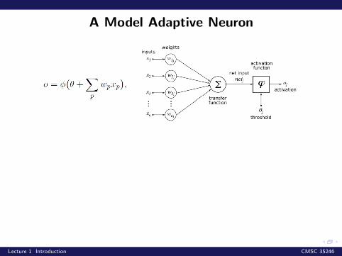
A Model Adaptive Neuron
This is also called a PerceptronAssumes data are linearly separable. Simple stochasticalgorithm for learning the linear classifierTheorem (Novikoff, 1962): Let w, w0 be a linear separatorwith ‖w‖ = 1, and margin γ. Then Perceptron will convergeafter
O((maxi ‖xi‖)2
γ2
)
Lecture 1 Introduction CMSC 35246

A Model Adaptive Neuron
This is also called a Perceptron
Assumes data are linearly separable. Simple stochasticalgorithm for learning the linear classifierTheorem (Novikoff, 1962): Let w, w0 be a linear separatorwith ‖w‖ = 1, and margin γ. Then Perceptron will convergeafter
O((maxi ‖xi‖)2
γ2
)
Lecture 1 Introduction CMSC 35246

A Model Adaptive Neuron
This is also called a PerceptronAssumes data are linearly separable. Simple stochasticalgorithm for learning the linear classifier
Theorem (Novikoff, 1962): Let w, w0 be a linear separatorwith ‖w‖ = 1, and margin γ. Then Perceptron will convergeafter
O((maxi ‖xi‖)2
γ2
)
Lecture 1 Introduction CMSC 35246

A Model Adaptive Neuron
This is also called a PerceptronAssumes data are linearly separable. Simple stochasticalgorithm for learning the linear classifierTheorem (Novikoff, 1962): Let w, w0 be a linear separatorwith ‖w‖ = 1, and margin γ. Then Perceptron will convergeafter
O((maxi ‖xi‖)2
γ2
)Lecture 1 Introduction CMSC 35246

Algorithm
Problem: Given a sequence of labeled examples(x1, y1), (x2, y2), . . . , where each xi ∈ Rd and yi ∈ {+1,−1},find a weight vector w and intercept b such thatsign(wxi + b) = yi for all i
Perceptron Algorithm
• initialize w = 0• if sign(wx) 6= y (mistake), then wnew = wold + ηyx (η
is learning rate)
Lecture 1 Introduction CMSC 35246

Algorithm
Problem: Given a sequence of labeled examples(x1, y1), (x2, y2), . . . , where each xi ∈ Rd and yi ∈ {+1,−1},find a weight vector w and intercept b such thatsign(wxi + b) = yi for all i
Perceptron Algorithm
• initialize w = 0
• if sign(wx) 6= y (mistake), then wnew = wold + ηyx (ηis learning rate)
Lecture 1 Introduction CMSC 35246

Algorithm
Problem: Given a sequence of labeled examples(x1, y1), (x2, y2), . . . , where each xi ∈ Rd and yi ∈ {+1,−1},find a weight vector w and intercept b such thatsign(wxi + b) = yi for all i
Perceptron Algorithm
• initialize w = 0• if sign(wx) 6= y (mistake), then wnew = wold + ηyx (η
is learning rate)
Lecture 1 Introduction CMSC 35246

Perceptron as a model of the brain?
Perceptron developed in the 1950s
Key publication: The perceptron: a probabilistic model forinformation storage and organization in the brain, FrankRosenblatt, Psychological Review, 1958
Goal: Pattern classification
From Mechanization of Thought Process (1959): “The Navyrevealed the embryo of an electronic computer today that itexpects will be able to walk, talk, see, write, reproduce itselfand be conscious of its existence. Later perceptrons will beable to recognize people and call out their names andinstantly translate speech in one language to speech andwriting in another language, it was predicted.”
Another ancient milestone: Hebbian learning rule (DonaldHebb, 1949)
Lecture 1 Introduction CMSC 35246

Perceptron as a model of the brain?
The Mark I perceptron machine was the first implementationof the perceptron algorithm.The machine was connected to a camera that used 2020cadmium sulfide photocells to produce a 400-pixel image. Themain visible feature is a patchboard that allowedexperimentation with different combinations of input features.To the right of that are arrays of potentiometers thatimplemented the adaptive weights
Lecture 1 Introduction CMSC 35246

Adaptive Neuron: Perceptron
A perceptron represents a decision surface in a d dimensionalspace as a hyperplane
Works only for those sets of examples that are linearlyseparable
Many boolean functions can be represented by a perceptron:AND, OR, NAND,NOR
Lecture 1 Introduction CMSC 35246

Adaptive Neuron: Perceptron
A perceptron represents a decision surface in a d dimensionalspace as a hyperplane
Works only for those sets of examples that are linearlyseparable
Many boolean functions can be represented by a perceptron:AND, OR, NAND,NOR
Lecture 1 Introduction CMSC 35246

Adaptive Neuron: Perceptron
A perceptron represents a decision surface in a d dimensionalspace as a hyperplane
Works only for those sets of examples that are linearlyseparable
Many boolean functions can be represented by a perceptron:AND, OR, NAND,NOR
Lecture 1 Introduction CMSC 35246
Problems?
If features are complex enough, anything can be classified
Thus features are really hand coded. But it comes with aclever algorithm for weight updates
If features are restricted, then some interesting tasks cannotbe learned and thus perceptrons are fundamentally limited inwhat they can do. Famous examples: XOR, Group InvarianceTheorems (Minsky, Papert, 1969)
Lecture 1 Introduction CMSC 35246

Coda
Single neurons are not able to solve complex tasks (lineardecision boundaries).
More layers of linear units are not enough (still linear).
We could have multiple layers of adaptive, non-linear hiddenunits. These are called Multi-layer perceptrons
Many local minima: Perceptron convergence theorem doesnot apply.
Intuitive conjecture in the 60s: There is no learning algorithmfor multilayer perceptrons
Lecture 1 Introduction CMSC 35246

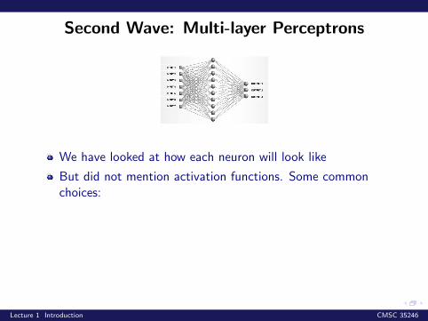
Second Wave: Multi-layer Perceptrons
We have looked at how each neuron will look like
But did not mention activation functions. Some commonchoices:
How can we learn the weights?
PS: There were many kinds of Neural Models explored in thesecond wave (will see later in the course)
Lecture 1 Introduction CMSC 35246

Learning multiple layers of features
[Slide: G. E. Hinton]
Lecture 1 Introduction CMSC 35246

Multilayer Perceptrons
Theoretical result [Cybenko, 1989]: 2-layer net with linearoutput can approximate any continuous function over compactdomain to arbitrary accuracy (given enough hidden units!)
The more number of hidden layers, the better...
.. in theory.
In practice deeper neural networks would need a lot of labeleddata and could be not trained easily
Neural Networks and Backpropagation (with the exception ofuse in Convolutional Networks) went out of fashion between1990-2006
Digression: Kernel Methods
Lecture 1 Introduction CMSC 35246

Return
In 2006 Hinton and colleagues found a way to pre-trainfeedforward networks using a Deep Belief Network trainedgreedily
This allowed larger networks to be trained by simply usingbackpropagation for fine tuning the pre-trained network(easier!)
Since 2010 pre-training of large feedforward networks in thissense also out
Availability of large datasets and fast GPU implementationshave made backpropagation from scratch almost unbeatable
Lecture 1 Introduction CMSC 35246
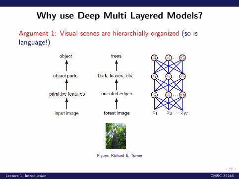
Why use Deep Multi Layered Models?
Argument 1: Visual scenes are hierarchially organized (so islanguage!)
Figure: Richard E. Turner
Lecture 1 Introduction CMSC 35246

Why use Deep Multi Layered Models?
Argument 2: Biological vision is hierarchically organized, and wewant to glean some ideas from there
Figure: Richard E. Turner
Lecture 1 Introduction CMSC 35246

In the perceptual system, neurons represent features of thesensory input
The brain learns to extract many layers of features. Featuresin one layer represent more complex combinations of featuresin the layer below. (e.g. Hubel Weisel (Vision), 1959, 1962)
How can we imitate such a process on a computer?
Lecture 1 Introduction CMSC 35246

Why use Deep Multi Layered Models?
Argument 3: Shallow representations are inefficient at representinghighly varying functions
when a function can be compactly represented by a deeparchitecture, it might need a very large architecture to berepresented by an insufficiently deep one
Is there a theoretical justification? No
Suggestive results:
Lecture 1 Introduction CMSC 35246

Why use Deep Multi Layered Models?
Argument 3: Shallow representations are inefficient at representinghighly varying functions
when a function can be compactly represented by a deeparchitecture, it might need a very large architecture to berepresented by an insufficiently deep one
Is there a theoretical justification?
No
Suggestive results:
Lecture 1 Introduction CMSC 35246

Why use Deep Multi Layered Models?
Argument 3: Shallow representations are inefficient at representinghighly varying functions
when a function can be compactly represented by a deeparchitecture, it might need a very large architecture to berepresented by an insufficiently deep one
Is there a theoretical justification? No
Suggestive results:
Lecture 1 Introduction CMSC 35246

Why use Deep Multi Layered Models?
Argument 3: Shallow representations are inefficient at representinghighly varying functions
when a function can be compactly represented by a deeparchitecture, it might need a very large architecture to berepresented by an insufficiently deep one
Is there a theoretical justification? No
Suggestive results:
Lecture 1 Introduction CMSC 35246

Why use Deep Multi Layered Models?
Argument 3: Shallow representations are inefficient at representinghighly varying functions
A two layer circuit of logic gates can represent any Booleanfunction (Mendelson, 1997)
First result: With depth-two logical circuits, most Booleanfunctions need an exponential number of logic gates
Another result (Hastad, 1986): There exist functions withpoly-size logic gate circuit of depth k that require exponentialsize when restricted to depth k − 1
Why do we care about boolean circuits?
Similar results are known when the computational units arelinear threshold units (Hastad, Razborov)
In practice depth helps in complicated tasks
Lecture 1 Introduction CMSC 35246

Why use Deep Multi Layered Models?
Attempt to learn features and the entire pipeline end-to-endrather than engineering it (the engineering focus shifts toarchitecture design)
[Figure: Honglak Lee]
Lecture 1 Introduction CMSC 35246

Convolutional Neural Networks
Figure: Yann LeCun
Lecture 1 Introduction CMSC 35246

Convolutional Neural Networks
Figure: Andrej Karpathy
Lecture 1 Introduction CMSC 35246

ImageNet Challenge 2012
14 million labeled images with 20,000 classes
Images gathered from the internet and labeled by humans viaAmazon Turk
Challenge: 1.2 million training images, 1000 classes.
Lecture 1 Introduction CMSC 35246

ImageNet Challenge 2012
14 million labeled images with 20,000 classes
Images gathered from the internet and labeled by humans viaAmazon Turk
Challenge: 1.2 million training images, 1000 classes.
Lecture 1 Introduction CMSC 35246

ImageNet Challenge 2012
14 million labeled images with 20,000 classes
Images gathered from the internet and labeled by humans viaAmazon Turk
Challenge: 1.2 million training images, 1000 classes.
Lecture 1 Introduction CMSC 35246

ImageNet Challenge 2012
Winning model (”AlexNet”) was a convolutional networksimilar to Yann LeCun, 1998
More data: 1.2 million versus a few thousand images
Fast two GPU implementation trained for a week
Better regularization[A. Krizhevsky, I. Sutskever, G. E. Hinton: ImageNet Classification with Deep Convolutional Neural Networks,NIPS 2012]
Lecture 1 Introduction CMSC 35246

Lecture 1 Introduction CMSC 35246
Going Deeper
A lot of current research has focussed on architecture(efficient, deeper, faster to train)
Examples: VGGNet, Inception, Highway Networks, ResidualNetworks, Fractal Networks
Lecture 1 Introduction CMSC 35246

Going Deeper
A lot of current research has focussed on architecture(efficient, deeper, faster to train)
Examples: VGGNet, Inception, Highway Networks, ResidualNetworks, Fractal Networks
Lecture 1 Introduction CMSC 35246

Going Deeper
Figure: Kaiming He, MSR
Lecture 1 Introduction CMSC 35246

Google LeNet
C. Szegedy et al, Going Deeper With Convolutions, CVPR 2015
Lecture 1 Introduction CMSC 35246

Revolution of Depth
K. He et al, Deep Residual Learning for Image Recognition, CVPR 2016. Slide: K. He
Lecture 1 Introduction CMSC 35246

Revolution of Depth
K. He et al, Deep Residual Learning for Image Recognition, CVPR 2016. Slide: K. He
Lecture 1 Introduction CMSC 35246

Residual Networks
Number 1 in Image classification
ImageNet Detection: 16 % better than the second best
ImageNet Localization: 27 % better than the second best
COCO Detection: 11 % better than the second best
COCO Segmentation: 12 % better than the second best
Lecture 1 Introduction CMSC 35246

Sequence Tasks
Figure credit: Andrej Karpathy
Lecture 1 Introduction CMSC 35246

Recent Deep Learning Successes and Research Areas
Lecture 1 Introduction CMSC 35246

2016: Year of Deep Learning
Lecture 1 Introduction CMSC 35246

Even Star Power! :)
Lecture 1 Introduction CMSC 35246

Maybe Hyped?
Lecture 1 Introduction CMSC 35246

Machine Translation
Your Google Translate usage will now be powered by an 8layer Long Short Term Memory Network with residualconnections and attention
Google’s Neural Machine Translation System: Bridging the Gap between Human and Machine Translation; Wu etal.
Lecture 1 Introduction CMSC 35246

Artistic Style
A Learned Representation for Artistic Style; Dumoulin, Shlens, Kudlur; ICLR 2017
Lecture 1 Introduction CMSC 35246

Speech Synthesis
Char2Wav: End-to-End Speech Synthesis; Sotelo et al., ICLR 2017; http://josesotelo.com/speechsynthesis/
Lecture 1 Introduction CMSC 35246

Game Playing
Mastering the game of Go with deep neural networks and tree search; Silver et al., Nature; 2016
Lecture 1 Introduction CMSC 35246

Neuroevolution of Architectures
Figure: @hardmaru
Recent large scale studies by Google show that evolutionarymethods are catching with intelligently designed architectures
Lecture 1 Introduction CMSC 35246

As well as in:
Protein Folding
Drug discovery
Particle Physics
Energy Management
...
Lecture 1 Introduction CMSC 35246

As well as in:
Protein Folding
Drug discovery
Particle Physics
Energy Management
...
Lecture 1 Introduction CMSC 35246

As well as in:
Protein Folding
Drug discovery
Particle Physics
Energy Management
...
Lecture 1 Introduction CMSC 35246

As well as in:
Protein Folding
Drug discovery
Particle Physics
Energy Management
...
Lecture 1 Introduction CMSC 35246

As well as in:
Protein Folding
Drug discovery
Particle Physics
Energy Management
...
Lecture 1 Introduction CMSC 35246

Next time
Feedforward Networks
Backpropagation
Lecture 1 Introduction CMSC 35246

Next time
Feedforward Networks
Backpropagation
Lecture 1 Introduction CMSC 35246