lecture 2 machine learning review - university of...
TRANSCRIPT
Lecture 2Machine Learning Review
CMSC 35246: Deep Learning
Shubhendu Trivedi&
Risi Kondor
University of Chicago
March 29, 2017
Lecture 2 Machine Learning Review CMSC 35246

Things we will look at today
• Formal Setup for Supervised Learning
• Empirical Risk, Risk, Generalization• Define and derive a linear model for Regression• Revise Regularization• Define and derive a linear model for Classification• (Time permitting) Start with Feedforward Networks
Lecture 2 Machine Learning Review CMSC 35246

Things we will look at today
• Formal Setup for Supervised Learning• Empirical Risk, Risk, Generalization
• Define and derive a linear model for Regression• Revise Regularization• Define and derive a linear model for Classification• (Time permitting) Start with Feedforward Networks
Lecture 2 Machine Learning Review CMSC 35246
Things we will look at today
• Formal Setup for Supervised Learning• Empirical Risk, Risk, Generalization• Define and derive a linear model for Regression
• Revise Regularization• Define and derive a linear model for Classification• (Time permitting) Start with Feedforward Networks
Lecture 2 Machine Learning Review CMSC 35246
Things we will look at today
• Formal Setup for Supervised Learning• Empirical Risk, Risk, Generalization• Define and derive a linear model for Regression• Revise Regularization
• Define and derive a linear model for Classification• (Time permitting) Start with Feedforward Networks
Lecture 2 Machine Learning Review CMSC 35246
Things we will look at today
• Formal Setup for Supervised Learning• Empirical Risk, Risk, Generalization• Define and derive a linear model for Regression• Revise Regularization• Define and derive a linear model for Classification
• (Time permitting) Start with Feedforward Networks
Lecture 2 Machine Learning Review CMSC 35246
Things we will look at today
• Formal Setup for Supervised Learning• Empirical Risk, Risk, Generalization• Define and derive a linear model for Regression• Revise Regularization• Define and derive a linear model for Classification• (Time permitting) Start with Feedforward Networks
Lecture 2 Machine Learning Review CMSC 35246

Note: Most slides in this presentation are adapted from, or taken(with permission) from slides by Professor Gregory Shakhnarovich
for his TTIC 31020 course
Lecture 2 Machine Learning Review CMSC 35246
What is Machine Learning?
Right question: What is learning?
Tom Mitchell (”Machine Learning”, 1997): ”A Computerprogram is said to learn from experience E with respect tosome class of tasks T and performance measure P , if itsperformance at tasks in T , as measured by P , improves withexperience E”
Gregory Shakhnarovich: Make predictions and pay the price ifthe predictions are incorrect. Goal of learning is to reduce theprice.
How can you specify T , P and E?
Lecture 2 Machine Learning Review CMSC 35246

Formal Setup (Supervised)
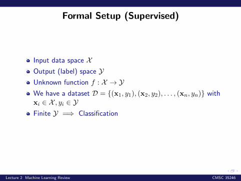
Input data space X
Output (label) space YUnknown function f : X → YWe have a dataset D = (x1, y1), (x2, y2), . . . , (xn, yn) withxi ∈ X , yi ∈ YFinite Y =⇒ Classification
Continuous Y =⇒ Regression
Lecture 2 Machine Learning Review CMSC 35246
Formal Setup (Supervised)
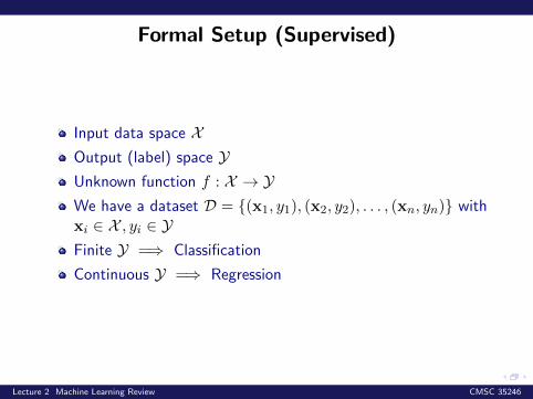
Input data space XOutput (label) space Y
Unknown function f : X → YWe have a dataset D = (x1, y1), (x2, y2), . . . , (xn, yn) withxi ∈ X , yi ∈ YFinite Y =⇒ Classification
Continuous Y =⇒ Regression
Lecture 2 Machine Learning Review CMSC 35246
Formal Setup (Supervised)
Input data space XOutput (label) space YUnknown function f : X → Y
We have a dataset D = (x1, y1), (x2, y2), . . . , (xn, yn) withxi ∈ X , yi ∈ YFinite Y =⇒ Classification
Continuous Y =⇒ Regression
Lecture 2 Machine Learning Review CMSC 35246
Formal Setup (Supervised)
Input data space XOutput (label) space YUnknown function f : X → YWe have a dataset D = (x1, y1), (x2, y2), . . . , (xn, yn) withxi ∈ X , yi ∈ Y
Finite Y =⇒ Classification
Continuous Y =⇒ Regression
Lecture 2 Machine Learning Review CMSC 35246
Formal Setup (Supervised)
Input data space XOutput (label) space YUnknown function f : X → YWe have a dataset D = (x1, y1), (x2, y2), . . . , (xn, yn) withxi ∈ X , yi ∈ YFinite Y =⇒ Classification
Continuous Y =⇒ Regression
Lecture 2 Machine Learning Review CMSC 35246
Formal Setup (Supervised)
Input data space XOutput (label) space YUnknown function f : X → YWe have a dataset D = (x1, y1), (x2, y2), . . . , (xn, yn) withxi ∈ X , yi ∈ YFinite Y =⇒ Classification
Continuous Y =⇒ Regression
Lecture 2 Machine Learning Review CMSC 35246
Regression
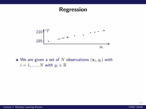
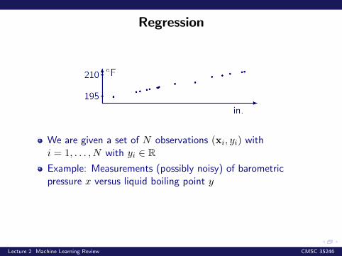
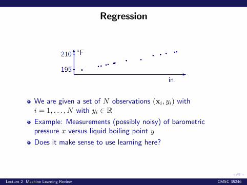
We are given a set of N observations (xi, yi) withi = 1, . . . , N with yi ∈ R
Example: Measurements (possibly noisy) of barometricpressure x versus liquid boiling point y
Does it make sense to use learning here?
Lecture 2 Machine Learning Review CMSC 35246
Regression
We are given a set of N observations (xi, yi) withi = 1, . . . , N with yi ∈ RExample: Measurements (possibly noisy) of barometricpressure x versus liquid boiling point y
Does it make sense to use learning here?
Lecture 2 Machine Learning Review CMSC 35246
Regression
We are given a set of N observations (xi, yi) withi = 1, . . . , N with yi ∈ RExample: Measurements (possibly noisy) of barometricpressure x versus liquid boiling point y
Does it make sense to use learning here?
Lecture 2 Machine Learning Review CMSC 35246
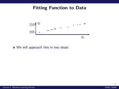
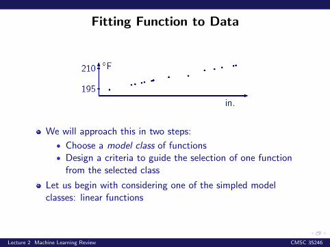
Fitting Function to Data
We will approach this in two steps:
• Choose a model class of functions• Design a criteria to guide the selection of one function
from the selected class
Let us begin with considering one of the simpled modelclasses: linear functions
Lecture 2 Machine Learning Review CMSC 35246
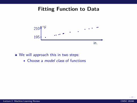
Fitting Function to Data
We will approach this in two steps:
• Choose a model class of functions
• Design a criteria to guide the selection of one functionfrom the selected class
Let us begin with considering one of the simpled modelclasses: linear functions
Lecture 2 Machine Learning Review CMSC 35246
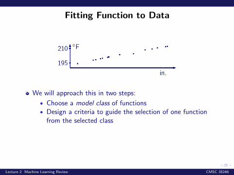
Fitting Function to Data
We will approach this in two steps:
• Choose a model class of functions• Design a criteria to guide the selection of one function
from the selected class
Let us begin with considering one of the simpled modelclasses: linear functions
Lecture 2 Machine Learning Review CMSC 35246
Linear Fitting to Data
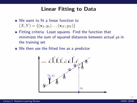
We want to fit a linear function to(X,Y ) = (x1, y1) . . . (xN , yN )
Fitting criteria: Least squares. Find the function thatminimizes the sum of squared distances between actual ys inthe training set
We then use the fitted line as a predictor
Lecture 2 Machine Learning Review CMSC 35246
Linear Fitting to Data
We want to fit a linear function to(X,Y ) = (x1, y1) . . . (xN , yN )Fitting criteria: Least squares. Find the function thatminimizes the sum of squared distances between actual ys inthe training set
We then use the fitted line as a predictor
Lecture 2 Machine Learning Review CMSC 35246
Linear Functions
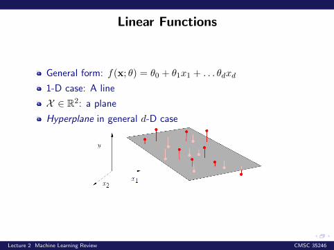
General form: f(x; θ) = θ0 + θ1x1 + . . . θdxd
1-D case: A line
X ∈ R2: a plane
Hyperplane in general d-D case
Lecture 2 Machine Learning Review CMSC 35246
Linear Functions
General form: f(x; θ) = θ0 + θ1x1 + . . . θdxd
1-D case: A line
X ∈ R2: a plane
Hyperplane in general d-D case
Lecture 2 Machine Learning Review CMSC 35246
Linear Functions
General form: f(x; θ) = θ0 + θ1x1 + . . . θdxd
1-D case: A line
X ∈ R2: a plane
Hyperplane in general d-D case
Lecture 2 Machine Learning Review CMSC 35246
Linear Functions
General form: f(x; θ) = θ0 + θ1x1 + . . . θdxd
1-D case: A line
X ∈ R2: a plane
Hyperplane in general d-D case
Lecture 2 Machine Learning Review CMSC 35246
Loss Functions
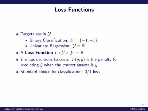
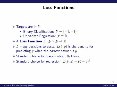
Targets are in Y• Binary Classification: Y = −1,+1• Univariate Regression: Y ≡ R
A Loss Function L : Y × Y → RL maps decisions to costs. L(y, y) is the penalty forpredicting y when the correct answer is y
Standard choice for classification: 0/1 loss
Standard choice for regression: L(y, y) = (y − y)2
Lecture 2 Machine Learning Review CMSC 35246
Loss Functions
Targets are in Y• Binary Classification: Y = −1,+1• Univariate Regression: Y ≡ R
A Loss Function L : Y × Y → R
L maps decisions to costs. L(y, y) is the penalty forpredicting y when the correct answer is y
Standard choice for classification: 0/1 loss
Standard choice for regression: L(y, y) = (y − y)2
Lecture 2 Machine Learning Review CMSC 35246
Loss Functions
Targets are in Y• Binary Classification: Y = −1,+1• Univariate Regression: Y ≡ R
A Loss Function L : Y × Y → RL maps decisions to costs. L(y, y) is the penalty forpredicting y when the correct answer is y
Standard choice for classification: 0/1 loss
Standard choice for regression: L(y, y) = (y − y)2
Lecture 2 Machine Learning Review CMSC 35246
Loss Functions
Targets are in Y• Binary Classification: Y = −1,+1• Univariate Regression: Y ≡ R
A Loss Function L : Y × Y → RL maps decisions to costs. L(y, y) is the penalty forpredicting y when the correct answer is y
Standard choice for classification: 0/1 loss
Standard choice for regression: L(y, y) = (y − y)2
Lecture 2 Machine Learning Review CMSC 35246
Empirical Loss
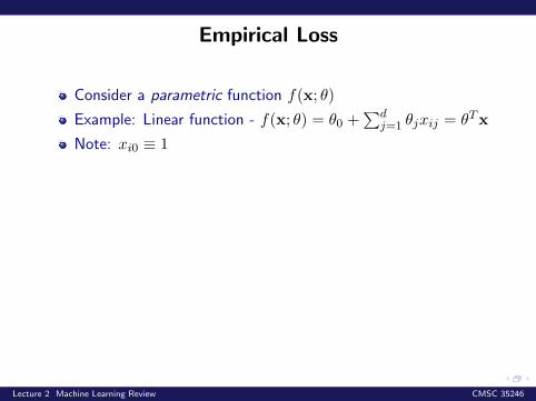
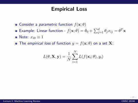
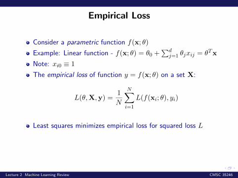
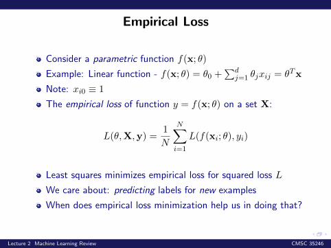
Consider a parametric function f(x; θ)
Example: Linear function - f(x; θ) = θ0 +∑d
j=1 θjxij = θTx
Note: xi0 ≡ 1
The empirical loss of function y = f(x; θ) on a set X:
L(θ,X,y) =1
N
N∑i=1
L(f(xi; θ), yi)
Least squares minimizes empirical loss for squared loss L
We care about: predicting labels for new examples
When does empirical loss minimization help us in doing that?
Lecture 2 Machine Learning Review CMSC 35246

Empirical Loss
Consider a parametric function f(x; θ)
Example: Linear function - f(x; θ) = θ0 +∑d
j=1 θjxij = θTx
Note: xi0 ≡ 1
The empirical loss of function y = f(x; θ) on a set X:
L(θ,X,y) =1
N
N∑i=1
L(f(xi; θ), yi)
Least squares minimizes empirical loss for squared loss L
We care about: predicting labels for new examples
When does empirical loss minimization help us in doing that?
Lecture 2 Machine Learning Review CMSC 35246
Loss: Empirical and Expected
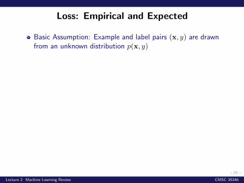
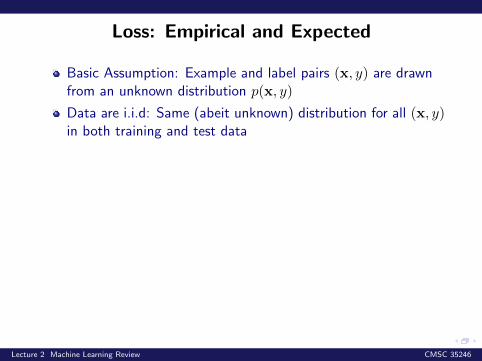
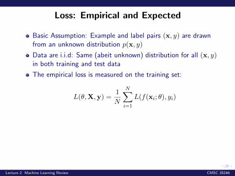
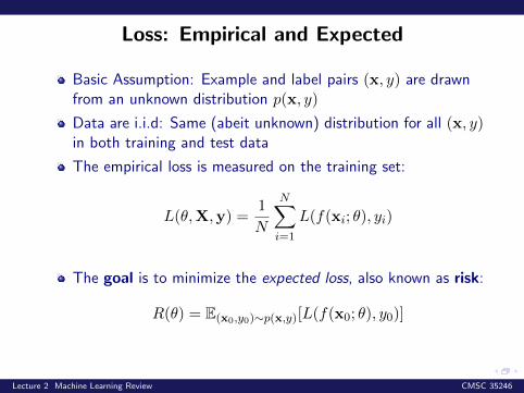
Basic Assumption: Example and label pairs (x, y) are drawnfrom an unknown distribution p(x, y)
Data are i.i.d: Same (abeit unknown) distribution for all (x, y)in both training and test data
The empirical loss is measured on the training set:
L(θ,X,y) =1
N
N∑i=1
L(f(xi; θ), yi)
The goal is to minimize the expected loss, also known as risk:
R(θ) = E(x0,y0)∼p(x,y)[L(f(x0; θ), y0)]
Lecture 2 Machine Learning Review CMSC 35246
Loss: Empirical and Expected
Basic Assumption: Example and label pairs (x, y) are drawnfrom an unknown distribution p(x, y)
Data are i.i.d: Same (abeit unknown) distribution for all (x, y)in both training and test data
The empirical loss is measured on the training set:
L(θ,X,y) =1
N
N∑i=1
L(f(xi; θ), yi)
The goal is to minimize the expected loss, also known as risk:
R(θ) = E(x0,y0)∼p(x,y)[L(f(x0; θ), y0)]
Lecture 2 Machine Learning Review CMSC 35246
Empirical Risk Minimization
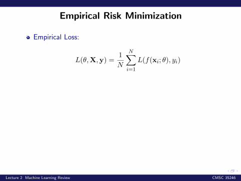
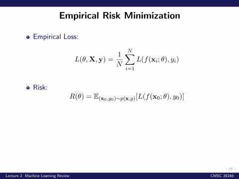
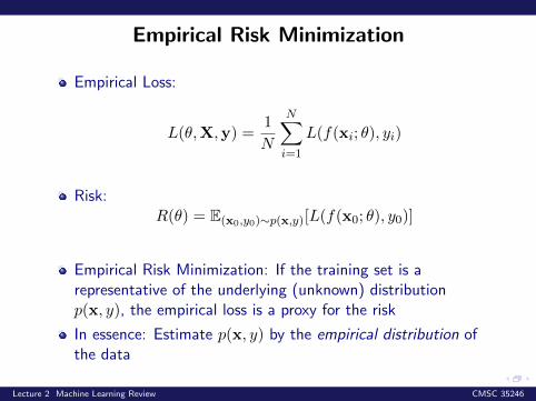
Empirical Loss:
L(θ,X,y) =1
N
N∑i=1
L(f(xi; θ), yi)
Risk:R(θ) = E(x0,y0)∼p(x,y)[L(f(x0; θ), y0)]
Empirical Risk Minimization: If the training set is arepresentative of the underlying (unknown) distributionp(x, y), the empirical loss is a proxy for the risk
In essence: Estimate p(x, y) by the empirical distribution ofthe data
Lecture 2 Machine Learning Review CMSC 35246
Empirical Risk Minimization
Empirical Loss:
L(θ,X,y) =1
N
N∑i=1
L(f(xi; θ), yi)
Risk:R(θ) = E(x0,y0)∼p(x,y)[L(f(x0; θ), y0)]
Empirical Risk Minimization: If the training set is arepresentative of the underlying (unknown) distributionp(x, y), the empirical loss is a proxy for the risk
In essence: Estimate p(x, y) by the empirical distribution ofthe data
Lecture 2 Machine Learning Review CMSC 35246

Learning via Empirical Loss Minimization
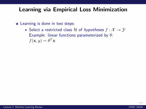
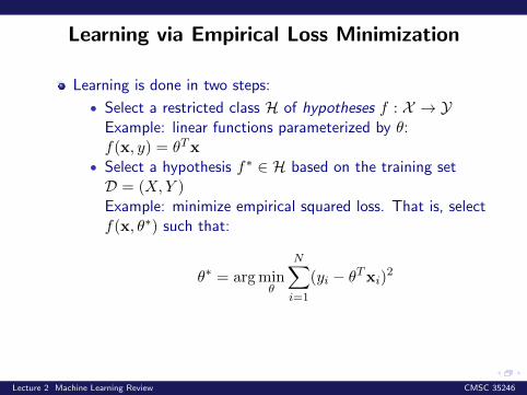
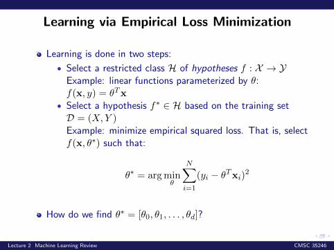
Learning is done in two steps:
• Select a restricted class H of hypotheses f : X → YExample: linear functions parameterized by θ:f(x, y) = θTx
• Select a hypothesis f∗ ∈ H based on the training setD = (X,Y )Example: minimize empirical squared loss. That is, selectf(x, θ∗) such that:
θ∗ = arg minθ
N∑i=1
(yi − θTxi)2
How do we find θ∗ = [θ0, θ1, . . . , θd]?
Lecture 2 Machine Learning Review CMSC 35246
Learning via Empirical Loss Minimization
Learning is done in two steps:
• Select a restricted class H of hypotheses f : X → YExample: linear functions parameterized by θ:f(x, y) = θTx
• Select a hypothesis f∗ ∈ H based on the training setD = (X,Y )Example: minimize empirical squared loss. That is, selectf(x, θ∗) such that:
θ∗ = arg minθ
N∑i=1
(yi − θTxi)2
How do we find θ∗ = [θ0, θ1, . . . , θd]?
Lecture 2 Machine Learning Review CMSC 35246
Least Squares: Estimation
Necessary condition to minimize L:∂L(θ)∂θ0
, ∂L(θ)∂θ1, . . . , ∂L(θ)∂θd
must be set to zero
Gives us d+ 1 linear equations in d+ 1 unknowns θ0, θ1, . . . , θd
Let us switch to vector notation for convenience
Lecture 2 Machine Learning Review CMSC 35246
Least Squares: Estimation
Necessary condition to minimize L:∂L(θ)∂θ0
, ∂L(θ)∂θ1, . . . , ∂L(θ)∂θd
must be set to zero
Gives us d+ 1 linear equations in d+ 1 unknowns θ0, θ1, . . . , θd
Let us switch to vector notation for convenience
Lecture 2 Machine Learning Review CMSC 35246
Least Squares: Estimation
Necessary condition to minimize L:∂L(θ)∂θ0
, ∂L(θ)∂θ1, . . . , ∂L(θ)∂θd
must be set to zero
Gives us d+ 1 linear equations in d+ 1 unknowns θ0, θ1, . . . , θd
Let us switch to vector notation for convenience
Lecture 2 Machine Learning Review CMSC 35246
Least Squares: Estimation
Necessary condition to minimize L:∂L(θ)∂θ0
, ∂L(θ)∂θ1, . . . , ∂L(θ)∂θd
must be set to zero
Gives us d+ 1 linear equations in d+ 1 unknowns θ0, θ1, . . . , θd
Let us switch to vector notation for convenience
Lecture 2 Machine Learning Review CMSC 35246
Learning via Empirical Loss Minimization
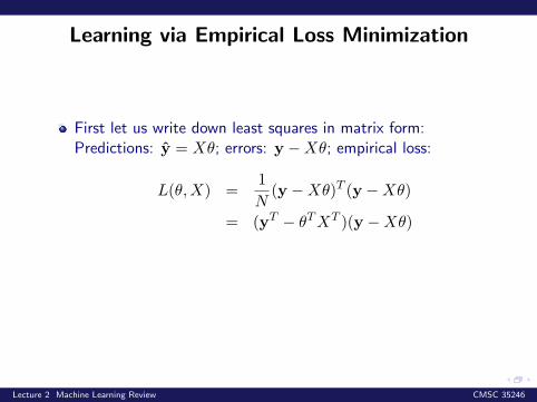
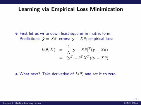
First let us write down least squares in matrix form:
Predictions: y = Xθ; errors: y −Xθ; empirical loss:
L(θ,X) =1
N(y −Xθ)T (y −Xθ)
= (yT − θTXT )(y −Xθ)
What next? Take derivative of L(θ) and set it to zero
Lecture 2 Machine Learning Review CMSC 35246
Learning via Empirical Loss Minimization
First let us write down least squares in matrix form:Predictions: y = Xθ;
errors: y −Xθ; empirical loss:
L(θ,X) =1
N(y −Xθ)T (y −Xθ)
= (yT − θTXT )(y −Xθ)
What next? Take derivative of L(θ) and set it to zero
Lecture 2 Machine Learning Review CMSC 35246
Learning via Empirical Loss Minimization
First let us write down least squares in matrix form:Predictions: y = Xθ; errors: y −Xθ;
empirical loss:
L(θ,X) =1
N(y −Xθ)T (y −Xθ)
= (yT − θTXT )(y −Xθ)
What next? Take derivative of L(θ) and set it to zero
Lecture 2 Machine Learning Review CMSC 35246
Learning via Empirical Loss Minimization
First let us write down least squares in matrix form:Predictions: y = Xθ; errors: y −Xθ; empirical loss:
L(θ,X) =1
N(y −Xθ)T (y −Xθ)
= (yT − θTXT )(y −Xθ)
What next? Take derivative of L(θ) and set it to zero
Lecture 2 Machine Learning Review CMSC 35246
Learning via Empirical Loss Minimization
First let us write down least squares in matrix form:Predictions: y = Xθ; errors: y −Xθ; empirical loss:
L(θ,X) =1
N(y −Xθ)T (y −Xθ)
= (yT − θTXT )(y −Xθ)
What next? Take derivative of L(θ) and set it to zero
Lecture 2 Machine Learning Review CMSC 35246
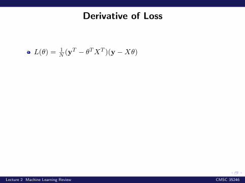
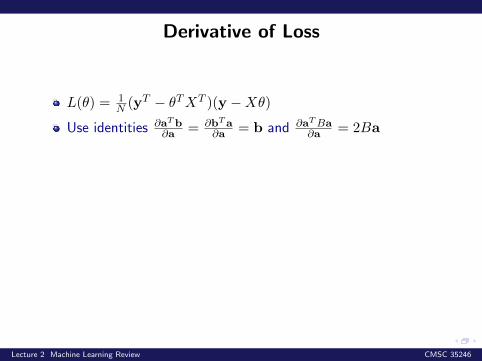
Derivative of Loss
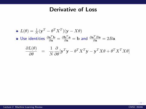
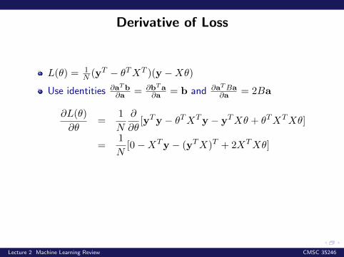
L(θ) = 1N (yT − θTXT )(y −Xθ)
Use identities ∂aTb∂a = ∂bT a
∂a = b and ∂aTBa∂a = 2Ba
∂L(θ)
∂θ=
1
N
∂
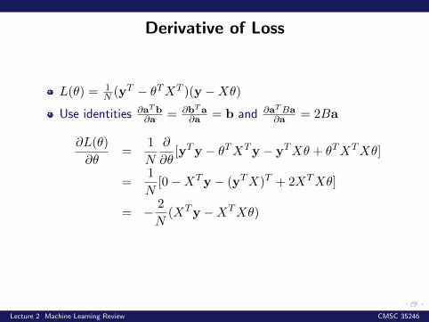
∂θ[yTy − θTXTy − yTXθ + θTXTXθ]
=1
N[0−XTy − (yTX)T + 2XTXθ]
= − 2
N(XTy −XTXθ)
Lecture 2 Machine Learning Review CMSC 35246
Derivative of Loss
L(θ) = 1N (yT − θTXT )(y −Xθ)
Use identities ∂aTb∂a = ∂bT a
∂a = b and ∂aTBa∂a = 2Ba
∂L(θ)
∂θ=
1
N
∂
∂θ[yTy − θTXTy − yTXθ + θTXTXθ]
=1
N[0−XTy − (yTX)T + 2XTXθ]
= − 2
N(XTy −XTXθ)
Lecture 2 Machine Learning Review CMSC 35246
Derivative of Loss
L(θ) = 1N (yT − θTXT )(y −Xθ)
Use identities ∂aTb∂a = ∂bT a
∂a = b and ∂aTBa∂a = 2Ba
∂L(θ)
∂θ=
1
N
∂
∂θ[yTy − θTXTy − yTXθ + θTXTXθ]
=1
N[0−XTy − (yTX)T + 2XTXθ]
= − 2
N(XTy −XTXθ)
Lecture 2 Machine Learning Review CMSC 35246
Derivative of Loss
L(θ) = 1N (yT − θTXT )(y −Xθ)
Use identities ∂aTb∂a = ∂bT a
∂a = b and ∂aTBa∂a = 2Ba
∂L(θ)
∂θ=
1
N
∂
∂θ[yTy − θTXTy − yTXθ + θTXTXθ]
=1
N[0−XTy − (yTX)T + 2XTXθ]
= − 2
N(XTy −XTXθ)
Lecture 2 Machine Learning Review CMSC 35246
Derivative of Loss
L(θ) = 1N (yT − θTXT )(y −Xθ)
Use identities ∂aTb∂a = ∂bT a
∂a = b and ∂aTBa∂a = 2Ba
∂L(θ)
∂θ=
1
N
∂
∂θ[yTy − θTXTy − yTXθ + θTXTXθ]
=1
N[0−XTy − (yTX)T + 2XTXθ]
= − 2
N(XTy −XTXθ)
Lecture 2 Machine Learning Review CMSC 35246
Least Squares Solution
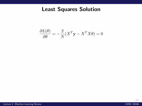
∂L(θ)
∂θ= − 2
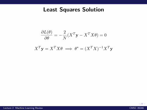
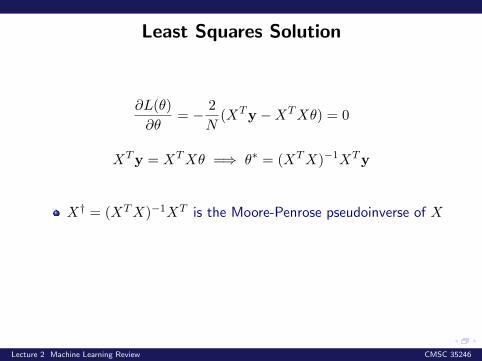
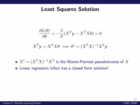
N(XTy −XTXθ) = 0
XTy = XTXθ =⇒ θ∗ = (XTX)−1XTy
X† = (XTX)−1XT is the Moore-Penrose pseudoinverse of X
Linear regression infact has a closed form solution!
Prediction: y = θ∗T
[1x0
]= yTX†
T
[1x0
]
Lecture 2 Machine Learning Review CMSC 35246
Least Squares Solution
∂L(θ)
∂θ= − 2
N(XTy −XTXθ) = 0
XTy = XTXθ =⇒ θ∗ = (XTX)−1XTy
X† = (XTX)−1XT is the Moore-Penrose pseudoinverse of X
Linear regression infact has a closed form solution!
Prediction: y = θ∗T
[1x0
]= yTX†
T
[1x0
]
Lecture 2 Machine Learning Review CMSC 35246
Least Squares Solution
∂L(θ)
∂θ= − 2
N(XTy −XTXθ) = 0
XTy = XTXθ =⇒ θ∗ = (XTX)−1XTy
X† = (XTX)−1XT is the Moore-Penrose pseudoinverse of X
Linear regression infact has a closed form solution!
Prediction: y = θ∗T
[1x0
]= yTX†
T
[1x0
]
Lecture 2 Machine Learning Review CMSC 35246
Least Squares Solution
∂L(θ)
∂θ= − 2
N(XTy −XTXθ) = 0
XTy = XTXθ =⇒ θ∗ = (XTX)−1XTy
X† = (XTX)−1XT is the Moore-Penrose pseudoinverse of X
Linear regression infact has a closed form solution!
Prediction: y = θ∗T
[1x0
]= yTX†
T
[1x0
]
Lecture 2 Machine Learning Review CMSC 35246

Least Squares Solution
∂L(θ)
∂θ= − 2
N(XTy −XTXθ) = 0
XTy = XTXθ =⇒ θ∗ = (XTX)−1XTy
X† = (XTX)−1XT is the Moore-Penrose pseudoinverse of X
Linear regression infact has a closed form solution!
Prediction: y = θ∗T
[1x0
]= yTX†
T
[1x0
]
Lecture 2 Machine Learning Review CMSC 35246
Polynomial Regression
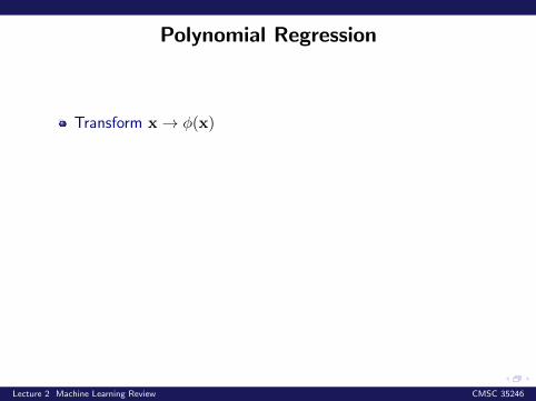
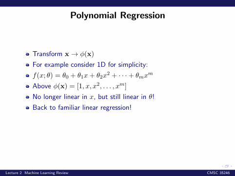
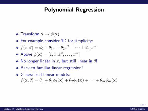
Transform x→ φ(x)
For example consider 1D for simplicity:
f(x; θ) = θ0 + θ1x+ θ2x2 + · · ·+ θmx
m
Above φ(x) = [1, x, x2, . . . , xm]
No longer linear in x, but still linear in θ!
Back to familiar linear regression!
Generalized Linear models:f(x; θ) = θ0 + θ1φ1(x) + θ2φ2(x) + · · ·+ θmφm(x)
Lecture 2 Machine Learning Review CMSC 35246
Polynomial Regression
Transform x→ φ(x)
For example consider 1D for simplicity:
f(x; θ) = θ0 + θ1x+ θ2x2 + · · ·+ θmx
m
Above φ(x) = [1, x, x2, . . . , xm]
No longer linear in x, but still linear in θ!
Back to familiar linear regression!
Generalized Linear models:f(x; θ) = θ0 + θ1φ1(x) + θ2φ2(x) + · · ·+ θmφm(x)
Lecture 2 Machine Learning Review CMSC 35246

A Short Primer on Regularization
Lecture 2 Machine Learning Review CMSC 35246
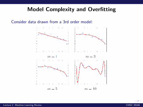
Model Complexity and Overfitting
Consider data drawn from a 3rd order model:
Lecture 2 Machine Learning Review CMSC 35246
Avoiding Overfitting: Cross Validation
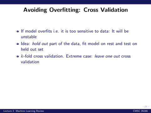
If model overfits i.e. it is too sensitive to data: It will beunstable
Idea: hold out part of the data, fit model on rest and test onheld out set
k-fold cross validation. Extreme case: leave one out crossvalidation
What is the source of overfitting?
Lecture 2 Machine Learning Review CMSC 35246

Avoiding Overfitting: Cross Validation
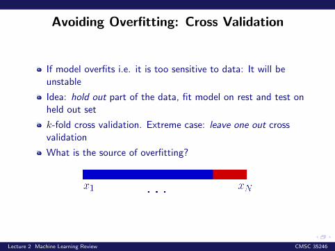
If model overfits i.e. it is too sensitive to data: It will beunstable
Idea: hold out part of the data, fit model on rest and test onheld out set
k-fold cross validation. Extreme case: leave one out crossvalidation
What is the source of overfitting?
Lecture 2 Machine Learning Review CMSC 35246
Avoiding Overfitting: Cross Validation
If model overfits i.e. it is too sensitive to data: It will beunstable
Idea: hold out part of the data, fit model on rest and test onheld out set
k-fold cross validation. Extreme case: leave one out crossvalidation
What is the source of overfitting?
Lecture 2 Machine Learning Review CMSC 35246
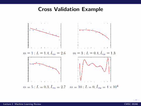
Cross Validation Example
Lecture 2 Machine Learning Review CMSC 35246

Model Complexity
Model complexity is the number of independent parameters tobe fit (”degrees of freedom”)
Complex model =⇒ more sensitive to data =⇒ more likelyto overfit
Simple model =⇒ more rigid =⇒ more likely to underfit
Find the model with the right ”bias-variance” balance
Lecture 2 Machine Learning Review CMSC 35246
Penalizing Model Complexity
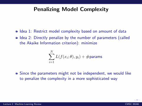
Idea 1: Restrict model complexity based on amount of data
Idea 2: Directly penalize by the number of parameters (calledthe Akaike Information criterion): minimize
N∑i=1
L(f(xi; θ), yi) + #params
Since the parameters might not be independent, we would liketo penalize the complexity in a more sophisticated way
Lecture 2 Machine Learning Review CMSC 35246
Penalizing Model Complexity
Idea 1: Restrict model complexity based on amount of data
Idea 2: Directly penalize by the number of parameters (calledthe Akaike Information criterion): minimize
N∑i=1
L(f(xi; θ), yi) + #params
Since the parameters might not be independent, we would liketo penalize the complexity in a more sophisticated way
Lecture 2 Machine Learning Review CMSC 35246
Problems
Lecture 2 Machine Learning Review CMSC 35246
Description Length
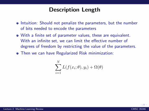
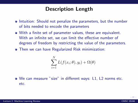
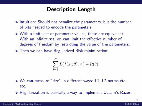
Intuition: Should not penalize the parameters, but the numberof bits needed to encode the parameters
With a finite set of parameter values, these are equivalent.With an infinite set, we can limit the effective number ofdegrees of freedom by restricting the value of the parameters.
Then we can have Regularized Risk minimization:
N∑i=1
L(f(xi; θ), yi) + Ω(θ)
We can measure ”size” in different ways: L1, L2 norms etc.etc.
Regularization is basically a way to implement Occam’s Razor
Lecture 2 Machine Learning Review CMSC 35246
Description Length
Intuition: Should not penalize the parameters, but the numberof bits needed to encode the parameters
With a finite set of parameter values, these are equivalent.With an infinite set, we can limit the effective number ofdegrees of freedom by restricting the value of the parameters.
Then we can have Regularized Risk minimization:
N∑i=1
L(f(xi; θ), yi) + Ω(θ)
We can measure ”size” in different ways: L1, L2 norms etc.etc.
Regularization is basically a way to implement Occam’s Razor
Lecture 2 Machine Learning Review CMSC 35246
Shrinkage Regression
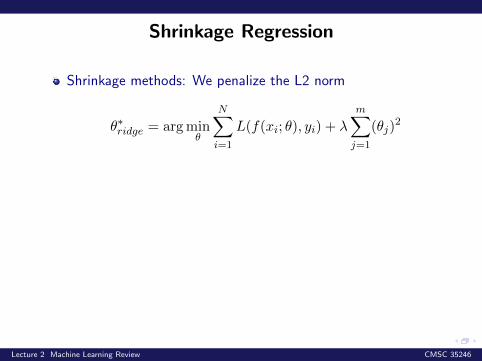
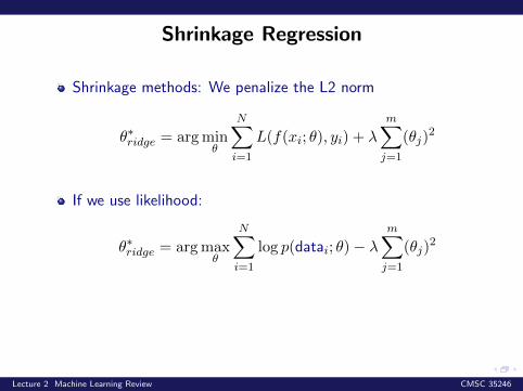
Shrinkage methods: We penalize the L2 norm
θ∗ridge = arg minθ
N∑i=1
L(f(xi; θ), yi) + λ
m∑j=1
(θj)2
If we use likelihood:
θ∗ridge = arg maxθ
N∑i=1
log p(datai; θ)− λm∑j=1
(θj)2
This is called Ridge regression: Closed form solution forsquared loss θridge = (λI +XTX)−1XTy!
Lecture 2 Machine Learning Review CMSC 35246
Shrinkage Regression
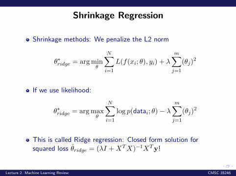
Shrinkage methods: We penalize the L2 norm
θ∗ridge = arg minθ
N∑i=1
L(f(xi; θ), yi) + λ
m∑j=1
(θj)2
If we use likelihood:
θ∗ridge = arg maxθ
N∑i=1
log p(datai; θ)− λm∑j=1
(θj)2
This is called Ridge regression: Closed form solution forsquared loss θridge = (λI +XTX)−1XTy!
Lecture 2 Machine Learning Review CMSC 35246
LASSO Regression
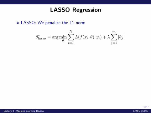
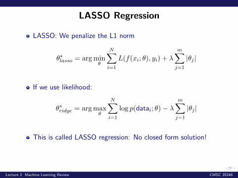
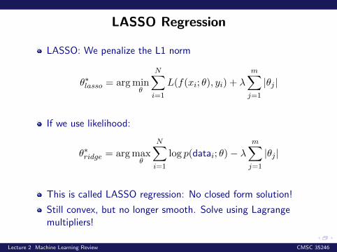
LASSO: We penalize the L1 norm
θ∗lasso = arg minθ
N∑i=1
L(f(xi; θ), yi) + λ
m∑j=1
|θj |
If we use likelihood:
θ∗ridge = arg maxθ
N∑i=1
log p(datai; θ)− λm∑j=1
|θj |
This is called LASSO regression: No closed form solution!
Still convex, but no longer smooth. Solve using Lagrangemultipliers!
Lecture 2 Machine Learning Review CMSC 35246
LASSO Regression
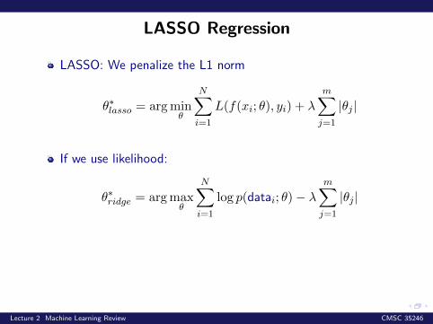
LASSO: We penalize the L1 norm
θ∗lasso = arg minθ
N∑i=1
L(f(xi; θ), yi) + λ
m∑j=1
|θj |
If we use likelihood:
θ∗ridge = arg maxθ
N∑i=1
log p(datai; θ)− λm∑j=1
|θj |
This is called LASSO regression: No closed form solution!
Still convex, but no longer smooth. Solve using Lagrangemultipliers!
Lecture 2 Machine Learning Review CMSC 35246
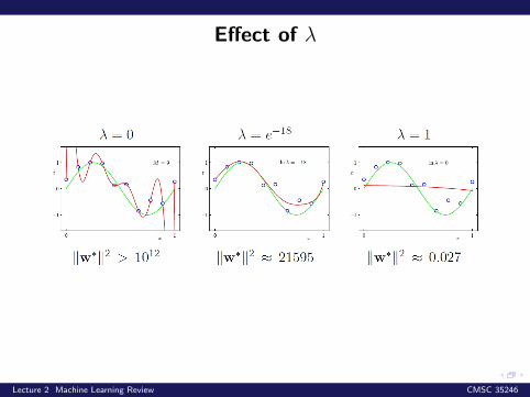
Effect of λ
Lecture 2 Machine Learning Review CMSC 35246
The Principle of Maximum Likelihood
Suppose we have N data points X = x1, x2, . . . , xN (or(x1, y1), (x2, y2), . . . , (xN , yN ))
Suppose we know the probability distribution function thatdescribes the data p(x; θ) (or p(y|x; θ))
Suppose we want to determine the parameter(s) θ
Pick θ so as to explain your data best
What does this mean?
Suppose we had two parameter values (or vectors) θ1 and θ2.
Now suppose you were to pretend that θ1 was really the truevalue parameterizing p. What would be the probability thatyou would get the dataset that you have? Call this P1
If P1 is very small, it means that such a dataset is veryunlikely to occur, thus perhaps θ1 was not a good guess
Lecture 2 Machine Learning Review CMSC 35246
The Principle of Maximum Likelihood
Suppose we have N data points X = x1, x2, . . . , xN (or(x1, y1), (x2, y2), . . . , (xN , yN ))Suppose we know the probability distribution function thatdescribes the data p(x; θ) (or p(y|x; θ))
Suppose we want to determine the parameter(s) θ
Pick θ so as to explain your data best
What does this mean?
Suppose we had two parameter values (or vectors) θ1 and θ2.
Now suppose you were to pretend that θ1 was really the truevalue parameterizing p. What would be the probability thatyou would get the dataset that you have? Call this P1
If P1 is very small, it means that such a dataset is veryunlikely to occur, thus perhaps θ1 was not a good guess
Lecture 2 Machine Learning Review CMSC 35246
The Principle of Maximum Likelihood
We want to pick θML i.e. the best value of θ that explains thedata you have
The plausibility of given data is measured by the ”likelihoodfunction” p(x; θ)
Maximum Likelihood principle thus suggests we pick θ thatmaximizes the likelihood function
The procedure:
• Write the log likelihood function: log p(x; θ) (we’ll seelater why log)
• Want to maximize - So differentiate log p(x; θ) w.r.t θand set to zero
• Solve for θ that satisfies the equation. This is θML
Lecture 2 Machine Learning Review CMSC 35246
The Principle of Maximum Likelihood
As an aside: Sometimes we have an initial guess for θBEFORE seeing the data
We then use the data to refine our guess of θ using BayesTheorem
This is called MAP (Maximum a posteriori) estimation (we’llsee an example)
Advantages of ML Estimation:
• Cookbook, ”turn the crank” method• ”Optimal” for large data sizes
Disadvantages of ML Estimation
• Not optimal for small sample sizes• Can be computationally challenging (numerical methods)
Lecture 2 Machine Learning Review CMSC 35246
Linear Classifiers
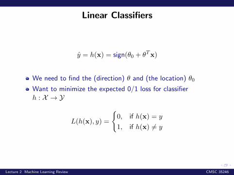
y = h(x) = sign(θ0 + θTx)
We need to find the (direction) θ and (the location) θ0
Want to minimize the expected 0/1 loss for classifierh : X → Y
L(h(x), y) =
0, if h(x) = y
1, if h(x) 6= y
Lecture 2 Machine Learning Review CMSC 35246
Linear Classifiers
y = h(x) = sign(θ0 + θTx)
We need to find the (direction) θ and (the location) θ0
Want to minimize the expected 0/1 loss for classifierh : X → Y
L(h(x), y) =
0, if h(x) = y
1, if h(x) 6= y
Lecture 2 Machine Learning Review CMSC 35246
Linear Classifiers
y = h(x) = sign(θ0 + θTx)
We need to find the (direction) θ and (the location) θ0
Want to minimize the expected 0/1 loss for classifierh : X → Y
L(h(x), y) =
0, if h(x) = y
1, if h(x) 6= y
Lecture 2 Machine Learning Review CMSC 35246
Risk of a Classifier
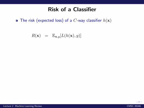
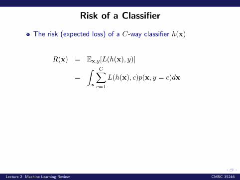
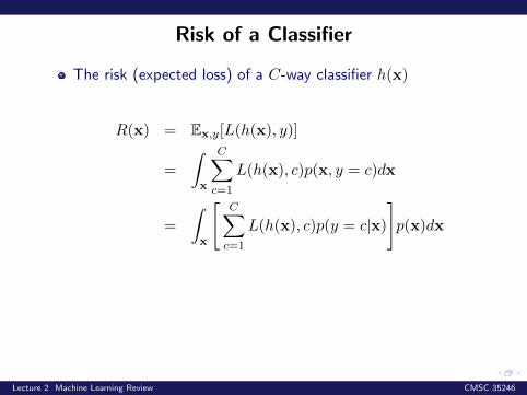
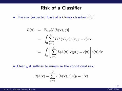
The risk (expected loss) of a C-way classifier h(x)
R(x) = Ex,y[L(h(x), y)]
=
∫x
C∑c=1
L(h(x), c)p(x, y = c)dx
=
∫x
[C∑c=1
L(h(x), c)p(y = c|x)
]p(x)dx
Clearly, it suffices to minimize the conditional risk:
R(h|x) =C∑c=1
L(h(x), c)p(y = c|x)
Lecture 2 Machine Learning Review CMSC 35246
Risk of a Classifier
The risk (expected loss) of a C-way classifier h(x)
R(x) = Ex,y[L(h(x), y)]
=
∫x
C∑c=1
L(h(x), c)p(x, y = c)dx
=
∫x
[C∑c=1
L(h(x), c)p(y = c|x)
]p(x)dx
Clearly, it suffices to minimize the conditional risk:
R(h|x) =
C∑c=1
L(h(x), c)p(y = c|x)
Lecture 2 Machine Learning Review CMSC 35246
Conditional Risk of a Classifier
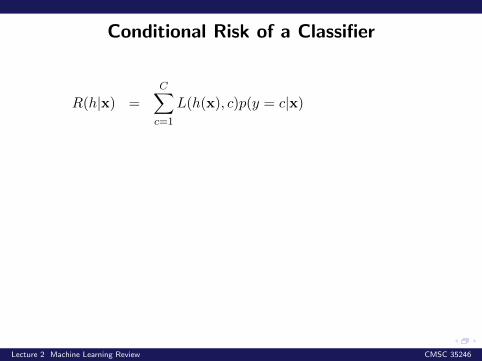
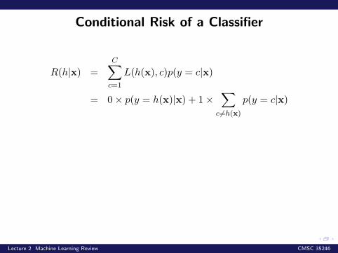
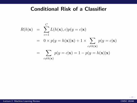
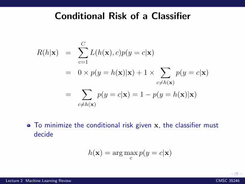
R(h|x) =
C∑c=1
L(h(x), c)p(y = c|x)
= 0× p(y = h(x)|x) + 1×∑
c 6=h(x)
p(y = c|x)
=∑
c 6=h(x)
p(y = c|x) = 1− p(y = h(x)|x)
To minimize the conditional risk given x, the classifier mustdecide
h(x) = arg maxcp(y = c|x)
Lecture 2 Machine Learning Review CMSC 35246
Conditional Risk of a Classifier
R(h|x) =
C∑c=1
L(h(x), c)p(y = c|x)
= 0× p(y = h(x)|x) + 1×∑
c 6=h(x)
p(y = c|x)
=∑
c 6=h(x)
p(y = c|x) = 1− p(y = h(x)|x)
To minimize the conditional risk given x, the classifier mustdecide
h(x) = arg maxcp(y = c|x)
Lecture 2 Machine Learning Review CMSC 35246
Conditional Risk of a Classifier
R(h|x) =
C∑c=1
L(h(x), c)p(y = c|x)
= 0× p(y = h(x)|x) + 1×∑
c 6=h(x)
p(y = c|x)
=∑
c 6=h(x)
p(y = c|x) = 1− p(y = h(x)|x)
To minimize the conditional risk given x, the classifier mustdecide
h(x) = arg maxcp(y = c|x)
Lecture 2 Machine Learning Review CMSC 35246
Conditional Risk of a Classifier
R(h|x) =
C∑c=1
L(h(x), c)p(y = c|x)
= 0× p(y = h(x)|x) + 1×∑
c 6=h(x)
p(y = c|x)
=∑
c 6=h(x)
p(y = c|x) = 1− p(y = h(x)|x)
To minimize the conditional risk given x, the classifier mustdecide
h(x) = arg maxcp(y = c|x)
Lecture 2 Machine Learning Review CMSC 35246

Log Odds Ratio
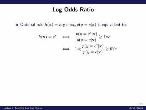
Optimal rule h(x) = arg maxc p(y = c|x) is equivalent to:
h(x) = c∗ ⇐⇒ p(y = c∗|x)
p(y = c|x)≥ 1∀c
⇐⇒ logp(y = c∗|x)
p(y = c|x)≥ 0∀c
For the binary case:
h(x) = 1 ⇐⇒ p(y = 1|x)
p(y = 0|x)≥ 0
Lecture 2 Machine Learning Review CMSC 35246
Log Odds Ratio
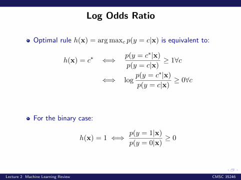
Optimal rule h(x) = arg maxc p(y = c|x) is equivalent to:
h(x) = c∗ ⇐⇒ p(y = c∗|x)
p(y = c|x)≥ 1∀c
⇐⇒ logp(y = c∗|x)
p(y = c|x)≥ 0∀c
For the binary case:
h(x) = 1 ⇐⇒ p(y = 1|x)
p(y = 0|x)≥ 0
Lecture 2 Machine Learning Review CMSC 35246
Log Odds Ratio
Optimal rule h(x) = arg maxc p(y = c|x) is equivalent to:
h(x) = c∗ ⇐⇒ p(y = c∗|x)
p(y = c|x)≥ 1∀c
⇐⇒ logp(y = c∗|x)
p(y = c|x)≥ 0∀c
For the binary case:
h(x) = 1 ⇐⇒ p(y = 1|x)
p(y = 0|x)≥ 0
Lecture 2 Machine Learning Review CMSC 35246
The Logistic Model
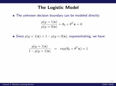
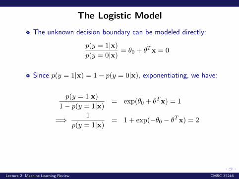
The unknown decision boundary can be modeled directly:
p(y = 1|x)
p(y = 0|x)= θ0 + θTx = 0
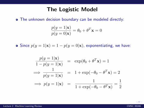
Since p(y = 1|x) = 1− p(y = 0|x), exponentiating, we have:
p(y = 1|x)
1− p(y = 1|x)= exp(θ0 + θTx) = 1
=⇒ 1
p(y = 1|x)= 1 + exp(−θ0 − θTx) = 2
=⇒ p(y = 1|x) =1
1 + exp(−θ0 − θTx)=
1
2
Lecture 2 Machine Learning Review CMSC 35246
The Logistic Model
The unknown decision boundary can be modeled directly:
p(y = 1|x)
p(y = 0|x)= θ0 + θTx = 0
Since p(y = 1|x) = 1− p(y = 0|x), exponentiating, we have:
p(y = 1|x)
1− p(y = 1|x)= exp(θ0 + θTx) = 1
=⇒ 1
p(y = 1|x)= 1 + exp(−θ0 − θTx) = 2
=⇒ p(y = 1|x) =1
1 + exp(−θ0 − θTx)=
1
2
Lecture 2 Machine Learning Review CMSC 35246
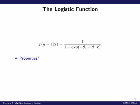
The Logistic Function
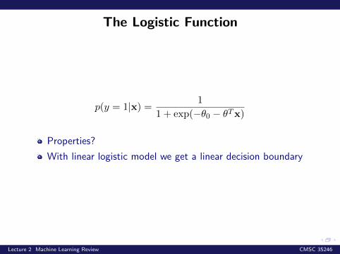
p(y = 1|x) =1
1 + exp(−θ0 − θTx)
Properties?
With linear logistic model we get a linear decision boundary
Lecture 2 Machine Learning Review CMSC 35246
The Logistic Function
p(y = 1|x) =1
1 + exp(−θ0 − θTx)
Properties?
With linear logistic model we get a linear decision boundary
Lecture 2 Machine Learning Review CMSC 35246
Likelihood under the Logistic Model
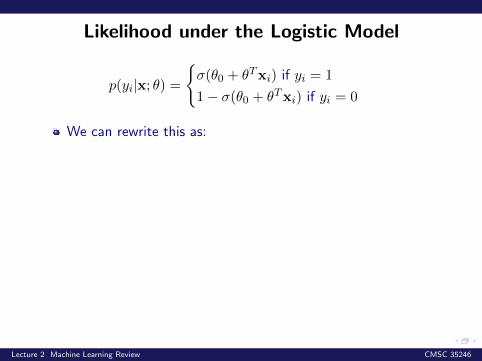
p(yi|x; θ) =
σ(θ0 + θTxi) if yi = 1
1− σ(θ0 + θTxi) if yi = 0
We can rewrite this as:
p(yi|x; θ) = σ(θ0 + θTxi)yi(1− σ(θ0 + θTxi))
1−yi
The log-likelihood of θ:
log p(Y |X; θ) =N∑i=1
log p(yi|xi; θ)
=N∑i=1
yi log σ(θ0 + θTxi) + (1− yi) log(1− σ(θ0 + θTxi))
Lecture 2 Machine Learning Review CMSC 35246
Likelihood under the Logistic Model
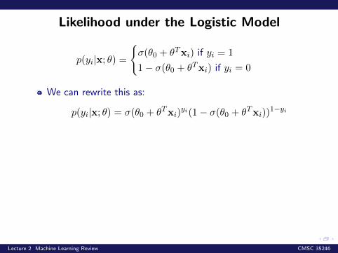
p(yi|x; θ) =
σ(θ0 + θTxi) if yi = 1
1− σ(θ0 + θTxi) if yi = 0
We can rewrite this as:
p(yi|x; θ) = σ(θ0 + θTxi)yi(1− σ(θ0 + θTxi))
1−yi
The log-likelihood of θ:
log p(Y |X; θ) =N∑i=1
log p(yi|xi; θ)
=N∑i=1
yi log σ(θ0 + θTxi) + (1− yi) log(1− σ(θ0 + θTxi))
Lecture 2 Machine Learning Review CMSC 35246
Likelihood under the Logistic Model
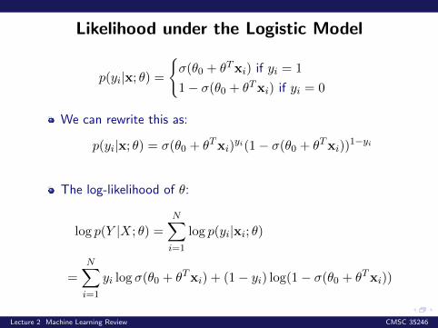
p(yi|x; θ) =
σ(θ0 + θTxi) if yi = 1
1− σ(θ0 + θTxi) if yi = 0
We can rewrite this as:
p(yi|x; θ) = σ(θ0 + θTxi)yi(1− σ(θ0 + θTxi))
1−yi
The log-likelihood of θ:
log p(Y |X; θ) =
N∑i=1
log p(yi|xi; θ)
=
N∑i=1
yi log σ(θ0 + θTxi) + (1− yi) log(1− σ(θ0 + θTxi))
Lecture 2 Machine Learning Review CMSC 35246
The Maximum Likelihood Solution
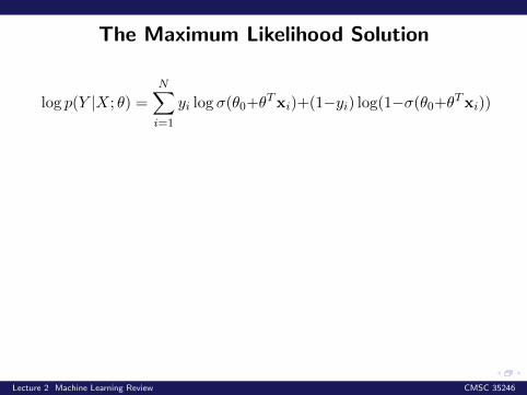
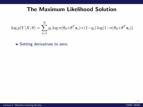
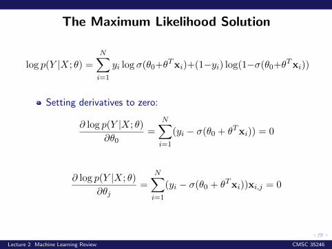
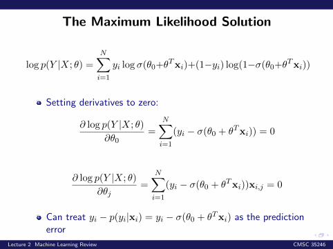
log p(Y |X; θ) =
N∑i=1
yi log σ(θ0+θTxi)+(1−yi) log(1−σ(θ0+θ
Txi))
Setting derivatives to zero:
∂ log p(Y |X; θ)
∂θ0=
N∑i=1
(yi − σ(θ0 + θTxi)) = 0
∂ log p(Y |X; θ)
∂θj=
N∑i=1
(yi − σ(θ0 + θTxi))xi,j = 0
Can treat yi − p(yi|xi) = yi − σ(θ0 + θTxi) as the predictionerror
Lecture 2 Machine Learning Review CMSC 35246
The Maximum Likelihood Solution
log p(Y |X; θ) =
N∑i=1
yi log σ(θ0+θTxi)+(1−yi) log(1−σ(θ0+θ
Txi))
Setting derivatives to zero:
∂ log p(Y |X; θ)
∂θ0=
N∑i=1
(yi − σ(θ0 + θTxi)) = 0
∂ log p(Y |X; θ)
∂θj=
N∑i=1
(yi − σ(θ0 + θTxi))xi,j = 0
Can treat yi − p(yi|xi) = yi − σ(θ0 + θTxi) as the predictionerror
Lecture 2 Machine Learning Review CMSC 35246
Finding Maxima
No closed form solution for the Maximum Likelihood for thismodel!
But log p(Y |X;x) is jointly concave in all components of θ
Or, equivalently, the error is convex
Gradient Descent/ascent (descent on − log p(y|x; θ), log loss)
Lecture 2 Machine Learning Review CMSC 35246
Finding Maxima
No closed form solution for the Maximum Likelihood for thismodel!
But log p(Y |X;x) is jointly concave in all components of θ
Or, equivalently, the error is convex
Gradient Descent/ascent (descent on − log p(y|x; θ), log loss)
Lecture 2 Machine Learning Review CMSC 35246
Finding Maxima
No closed form solution for the Maximum Likelihood for thismodel!
But log p(Y |X;x) is jointly concave in all components of θ
Or, equivalently, the error is convex
Gradient Descent/ascent (descent on − log p(y|x; θ), log loss)
Lecture 2 Machine Learning Review CMSC 35246
Finding Maxima
No closed form solution for the Maximum Likelihood for thismodel!
But log p(Y |X;x) is jointly concave in all components of θ
Or, equivalently, the error is convex
Gradient Descent/ascent (descent on − log p(y|x; θ), log loss)
Lecture 2 Machine Learning Review CMSC 35246

Next time
Feedforward Networks
Backpropagation
Lecture 2 Machine Learning Review CMSC 35246

Next time
Feedforward Networks
Backpropagation
Lecture 2 Machine Learning Review CMSC 35246