6.003: Signals and Systems

Feedback and Control

October 13, 2011 1

2

Courtesy of Jason Dorfman MIT / CSAIL. Used with permission.

Example: Perching

Can we make a fixed-wing UAV land on a perch like a bird?

3

The “Perching” Problem

4

Courtesy of Leon van Dommelen and Szu-Chuan Wang. Used with permission.

Photo from Naval Historical Center Aircraft Data Series.

Photo of a cardinal landing on a branch removed due to copyright restrictions.

Dimensionless Analysis

• Bird or plane...

• with mass m, wing area S, operating in a fluid with density ρ

• which requires a distance x to slow from V0 to Vf

• Distance-averaged drag coefficient, CD:

2m �

V0 �

�CD� = ln ρSx Vf

• A few (very preliminary) reference points:

Vehicle Average CD

Boeing 747 0.16

X-31 0.3

Cornell Perching Plane 0.25

Common Pigeon 10

5

Photo of the Boeing 747-400ER removed due to copyright restrictions.

U.S. Navy photo by James Darcy.Photos of Cornell perching plane and landing pigeon removed due to copyright restrictions.

6

Image removed due to copyright restrictions. Please see SlowMoHighSpeed. "Photron SA2 Camera - Eagle Owl in Flight."October 27, 2008. YouTube. Accessed September 25, 2012. http://www.youtube.com/watch?v=LA6XSrM0V_0

Experiment Design

• Glider (no propellor)

• Flat plate wings

• Dihedral (passive roll stability)

• Offboard sensing and control

7

System Identification

• Nonlinear rigid-body vehicle model

• Linear actuator model (+ saturations, delay)

• Real flight data (no wind tunnel)

8

System Identification

Lift Coefficient Drag Coefficient

1

1.5 Glider Data Flat Plate Theory

3

3.5 Glider Data Flat Plate Theory

2.5

0.5 2

Cl 0 Cd 1.5

1 −0.5

0.5

−1 0

−20−1.5

0 20 40 60 80 Angle of Attack

100 120 140 160 −20−0.5

0 20 40 60 80 Angle of Attack

100 120 140 160

9

A Dynamic Model

(x, z)m, I

!F

F

g

w

e l

lw

el

• Planar dynamics

• Aerodynamics fit from data

• State: x = [x, y, θ, φ, x,˙ y,˙ θ̇]

• Actuator: u = φ̇

10

Perching Results

• Enters motion capture @ 6m/s

• Perch in < 3.5m away Requires separation!

• Entire trajectory < 1s

11

Flow visualization

12

Courtesy of Jason Dorfman MIT / CSAIL. Used with permission.

Dimensionless Analysis

Vehicle Average CD

Boeing 747 0.16

X-31 0.3

Cornell Perching Plane 0.25

Common Pigeon 10

Our glider 1.1

Cobra maneuver (Mig) 0.9

13

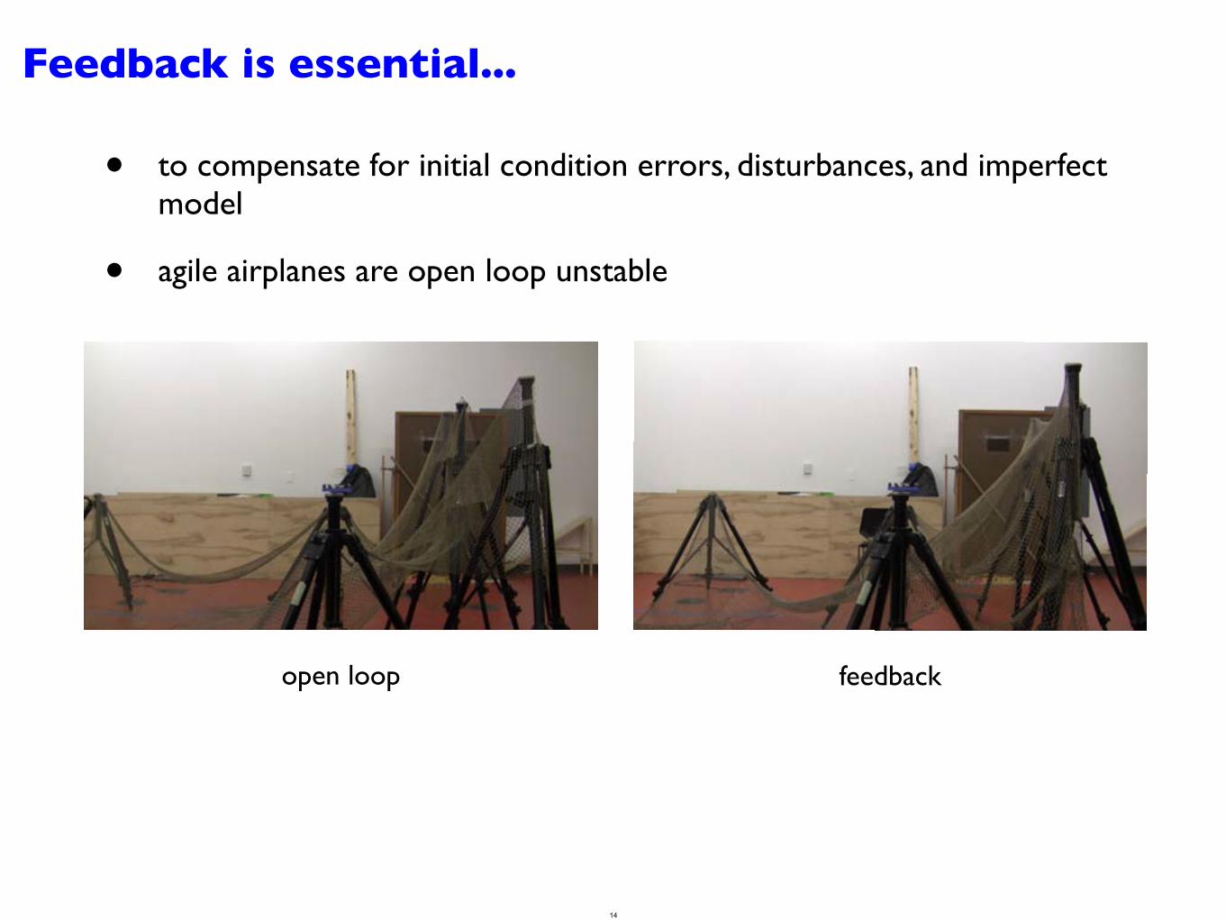
Feedback is essential...

• to compensate for initial condition errors, disturbances, and imperfect model

• agile airplanes are open loop unstable

open loop feedback

14

Today’s goal

Use systems theory to gain insight into how to control a system.

15

Example: wallFinder System

Approach a wall, stopping a desired distance di in front of it.

di = desiredFrontdo = distanceFront

t

do

K = −0.5 t

do

K = −1

t

do

K = −2 t

do

K = −8

What causes these different types of responses?

16

Structure of a Control Problem

(Simple) Control systems have three parts.

The plant is the system to be controlled.

The sensor measures the output of the plant.

The controller specifies a command C to the plant based on the

difference between the input X and sensor output S.

+−

X YE

S

C

controller plant

sensor

17

Analysis of wallFinder System

Cast wallFinder problem into control structure.

+−

X YE

S

C

controller plant

sensor

di = desiredFrontdo = distanceFront

proportional controller: v[n] = Ke[n] = K di[n] − ds[n]

locomotion: do[n] = do[n − 1] − Tv[n − 1]

sensor with no delay: ds[n] = do[n] 18

Analysis of wallFinder System: Block Diagram

Visualize as block diagram.

di = desiredFrontdo = distanceFront

proportional controller: v[n] = Ke[n] = K di[n] − ds[n]

locomotion: do[n] = do[n − 1] − Tv[n − 1]

sensor with no delay: ds[n] = do[n]

+ K −T + RDi Do−

V

19

( )

Analysis of wallFinder System: System Function

Solve.

di = desiredFrontdo = distanceFront

+ K −T + RDi Do−

V

−KT R Do 1 − R −KT R −KT R = = = Di 1 − R − KT R 1 − (1 + KT )R1 +

−KT R 1 − R

20

Analysis of wallFinder System: Poles

The system function contains a single pole at z = 1 + KT . Do −KT R = Di 1 − (1 + KT )R

Unit-sample response for KT = −0.2:

0n

h[n]

0.2

Unit-step response s[n] for KT = −0.2:

1

0n

What determines the speed of the response? Could it be faster? 21

Check Yourself

Find KT for fastest convergence of unit-sample response.

Do

Di =

−KT R 1 − (1 + KT )R

1. KT = −2

2. KT = −1

3. KT = 0

4. KT = 1

5. KT = 2

0. none of the above

22

Check Yourself

Find KT for fastest convergence of unit-sample response.

Do −KT R = Di 1 − (1 + KT )R

If KT = −1 then the pole is at z = 0.

Do −KT R = = R Di 1 − (1 + KT )R

Unit-sample response has a single non-zero output sample, at n = 1.

23

Analysis of wallFinder System: Poles

The poles of the system function provide insight for choosing K.

Do −KT R (1 − po)R Di

= 1 − (1 + KT )R = 1 − poR

; p0 = 1 + KT

1 Re z

Im z

0 < p0 < 1−1 < KT < 0monotonicconverging

1 Re z

Im z

−1 < p0 < 0−2 < KT < −1

alternating

converging

1 Re z

Im z

p0 < −1KT < −2

alternating

diverging

24

Check Yourself

Find KT for fastest convergence of unit-sample response.

Do

Di =

−KT R 1 − (1 + KT )R

1. KT = −2

2. KT = −1

3. KT = 0

4. KT = 1

5. KT = 2

0. none of the above

25

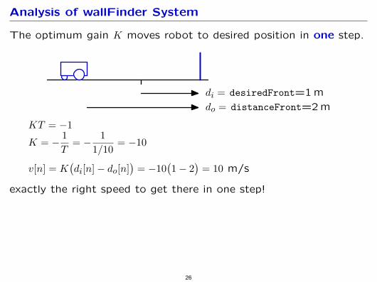
Analysis of wallFinder System

The optimum gain K moves robot to desired position in one step.

di = desiredFront=1 m

do = distanceFront=2 m

KT = −1 1 1

K = − = − = −10 T 1/10

v[n] = K di[n] − do[n] = −10 1 − 2 = 10 m/s

exactly the right speed to get there in one step!

26

( ) ( )

Analyzing wallFinder: Space-Time Diagram

The optimum gain K moves robot to desired position in one step.

di = desiredFrontdo = distanceFront

position

time

v = 10

27

Analyzing wallFinder: Space-Time Diagram

The optimum gain K moves robot to desired position in one step.

di = desiredFrontdo = distanceFront

position

time

v = 10v = 0

28

Analyzing wallFinder: Space-Time Diagram

The optimum gain K moves robot to desired position in one step.

di = desiredFrontdo = distanceFront

position

time

v = 10v = 0v = 0v = 0v = 0v = 0v = 0

29

Analysis of wallFinder System: Adding Sensor Delay

Adding delay tends to destabilize control systems.

di = desiredFrontdo = distanceFront

proportional controller: v[n] = Ke[n] = K di[n] − ds[n]

locomotion: do[n] = do[n − 1] − Tv[n − 1]

sensor with delay: ds[n] = do[n − 1]

30

( )

Analysis of wallFinder System: Adding Sensor Delay

Adding delay tends to destabilize control systems.

di = desiredFrontdo = distanceFront

position

time

v = 10

31

Analysis of wallFinder System: Adding Sensor Delay

Adding delay tends to destabilize control systems.

di = desiredFrontdo = distanceFront

position

time

v = 10v = 0

32

Analysis of wallFinder System: Adding Sensor Delay

Adding delay tends to destabilize control systems.

di = desiredFrontdo = distanceFront

position

time

v = 10v = 0v = −10

33

Analysis of wallFinder System: Adding Sensor Delay

Adding delay tends to destabilize control systems.

di = desiredFrontdo = distanceFront

position

time

v = 10v = 0v = −10v = −10

34

Analysis of wallFinder System: Adding Sensor Delay

Adding delay tends to destabilize control systems.

di = desiredFrontdo = distanceFront

position

time

v = 10v = 0v = −10v = −10v = 0

35

Analysis of wallFinder System: Block Diagram

Incorporating sensor delay in block diagram.

di = desiredFrontdo = distanceFront

proportional controller: v[n] = Ke[n] = K di[n] − ds[n]

locomotion: do[n] = do[n − 1] − Tv[n − 1]

sensor with no delay: ds[n] = do[n − 1]

+ K −T + R

R

Di Do−

V

36

( )

Check Yourself

Find the system function H = Do

Di .

+ K −T + R

R

Di Do−

V

1. KT R 1 − R

2. −KT R

1 + R − KT R2

3. KT R 1 − R

− KT R 4. −KT R

1 − R − KT R2

5. none of the above

37

Check Yourself

Do

Do

Di 1 − R − KT R2 1 +

−KT R2

Find the system function H = Di

.

+ K −T + R

R

Di Do−

V

Replace accumulator with equivalent block diagram.

+ K −T R1−R

R

Di Do−

=

−KT R 1 − R =

−KT R

1 − R

38

Check Yourself

Find the system function H = Do

Di .

+ K −T + R

R

Di Do−

V

1. KT R 1 − R

2. −KT R

1 + R − KT R2

3. KT R 1 − R

− KT R 4. −KT R

1 − R − KT R2

5. none of the above

39

Analyzing wallFinder: Poles

1 Substitute R → in the system functional to find the poles.

z

Do −KT R −KT 1 −KTz z= = = Di 1 − R − KT R2 1 − 1

z − KT 1 2 z2 − z − KT

z

The poles are then the roots of the denominator. a 21 1 z = + KT 2

± 2

40

� �

Feedback and Control: Poles

If KT is small, the poles are at z ≈ −KT and z ≈ 1 + KT .

2+ KT ≈ 12 ± + KT

2 = 1 + KT, −KT 12

1 Re z

Im zz-planeKT ≈ 0

Pole near 0 generates fast response.

z = 12 ± 1

2

Pole near 1 generates slow response.

Slow mode (pole near 1) dominates the response. 41

� �

Feedback and Control: Poles

As KT becomes more negative, the poles move toward each other

and collide at z = when KT = − . 12

14

z = 12 ±

212 + KT = 1

2 ± 12 − = , 1

4 12

12

21 Re z

Im zz-plane

KT = −14

Persistent responses decay. The system is stable.

2

42

( ) ( )

� �

Feedback and Control: Poles

If KT < −1/4, the poles are complex.

2+ KT = 12 ± j −KT − 1

2

1 Re z

Im zz-planeKT = −1

Complex poles → oscillations.

z = 12 ± 1

2 2

43

( ) ( )

Same oscillation we saw earlier!

Adding delay tends to destabilize control systems.

di = desiredFrontdo = distanceFront

position

time

v = 10v = 0v = −10v = −10v = 0

44

Check Yourself

1 Re z

Im zz-planeKT = −1

What is the period of the oscillation?

1. 1 2. 2 3. 3

4. 4 5. 6 0. none of above

45

Check Yourself

1 Re z

Im zz-planeKT = −1

√1 3 ±jπ/3 p0 = 2

± j = e2 n ±jπn/3 p = e0

±j0π/3 ±jπ/3 ±j2π/3 ±j3π/3 ±j4π/3 ±j5π/3 ±j6π/3 e , e , e , e , e , e , ee -v " e -v " 1 e±j2π=1

46

Check Yourself

1 Re z

Im zz-planeKT = −1

What is the period of the oscillation?

1. 1 2. 2 3. 3

4. 4 5. 6 0. none of above

47

Feedback and Control: Poles

If KT : 0 → −∞:

The closed loop poles depend on the gain.

1 Re z

Im zz-plane

then z1, z2 : 0, 1 → 1 2 , 2 → 1

2 ± j∞1

48

Check Yourself

Find KT for fastest response.

1 Re z

Im zz-plane

closed-loop poles

12 ±

√(12

)2+KT

1. 0 2. −14 3. −1

2 4. −1 5. −∞ 0. none of above

49

Check Yourself a 211 + KT z = ±2 2

The dominant pole always has a magnitude that is ≥ .

1 2.It is smallest when there is a double pole at z =

Therefore, KT = − 1 4.

1 2

50

( )

Check Yourself

Find KT for fastest response.

1 Re z

Im zz-plane

closed-loop poles

12 ±

√(12

)2+KT

1. 0 2. −14 3. −1

2 4. −1 5. −∞ 0. none of above

51

Destabilizing Effect of Delay

Adding delay in the feedback loop makes it more difficult to stabilize.

Ideal sensor: ds[n] = do[n]

More realistic sensor (with delay): ds[n] = do[n − 1]

1 Re z

Im z

1 Re z

Im z

Fastest response without delay: single pole at z = 0. 1

Fastest response with delay: double pole at z = much slower! 2 .

52

Destabilizing Effect of Delay

Adding more delay in the feedback loop is even worse.

More realistic sensor (with delay): ds[n] = do[n − 1]

Even more delay: ds[n] = do[n − 2]

1 Re z

Im z

21 Re z

Im z

Fastest response with delay: double pole at z = 1 2 .

Fastest response with more delay: double pole at z = 0.682.

→ even slower 53

Feedback and Control: Summary

Feedback is an elegant way to design a control system.

Stability of a feedback system is determined by its dominant pole.

Delays tend to decrease the stability of a feedback system.

54

55

Photo from Naval Historical Center Aircraft Data Series.

56

Block diagram of the F-14 control system as modeled in Simulink® removed due to copyright restrictions. Please see "F-14 Longitudinal Flight Control." The MathWorks, Inc.

MIT OpenCourseWarehttp://ocw.mit.edu

6.003 Signals and SystemsFall 2011

For information about citing these materials or our Terms of Use, visit: http://ocw.mit.edu/terms.