lecture 14. ht and ci for two means (2)

7/28/2019 Lecture 14. HT and CI for Two Means (2)

http://slidepdf.com/reader/full/lecture-14-ht-and-ci-for-two-means-2 1/85

Statistics

ST 361: Introduction to StatisticsHypothesis tests and Confidence

Intervals for two means

Kimberly [email protected]



Statistics 3

Recall: The Basic Paradigm.

•Population •Sample

•Statistics

•Inference

•Parameters



Statistics

Now, Compare two groups

• Group 1 • Group 2



Statistics 5

Inference for differences

•Population 1 •Sample 1

•Statistics

•Inference

•Parameters

•Population 2 •Sample 2

•Statistics

•Inference

•Parameters

•Inference•Difference in parameters •Difference in statistics



Statistics

Hypothetical situation

• Population A – Mean 300, standard deviation 100

• Population B

– Mean 100, standard deviation 30 • Sample from both populations

– n=30

• Calculate the mean of both samples • Take the difference in the means



Statistics

Hypothetical situation

• Sample A mean=323.8 • Sample B mean = 98.1 • Difference = 225.6

• Repeat this process 10000 times



Statistics

Means of sample A



Statistics

Means of sample B



Statistics

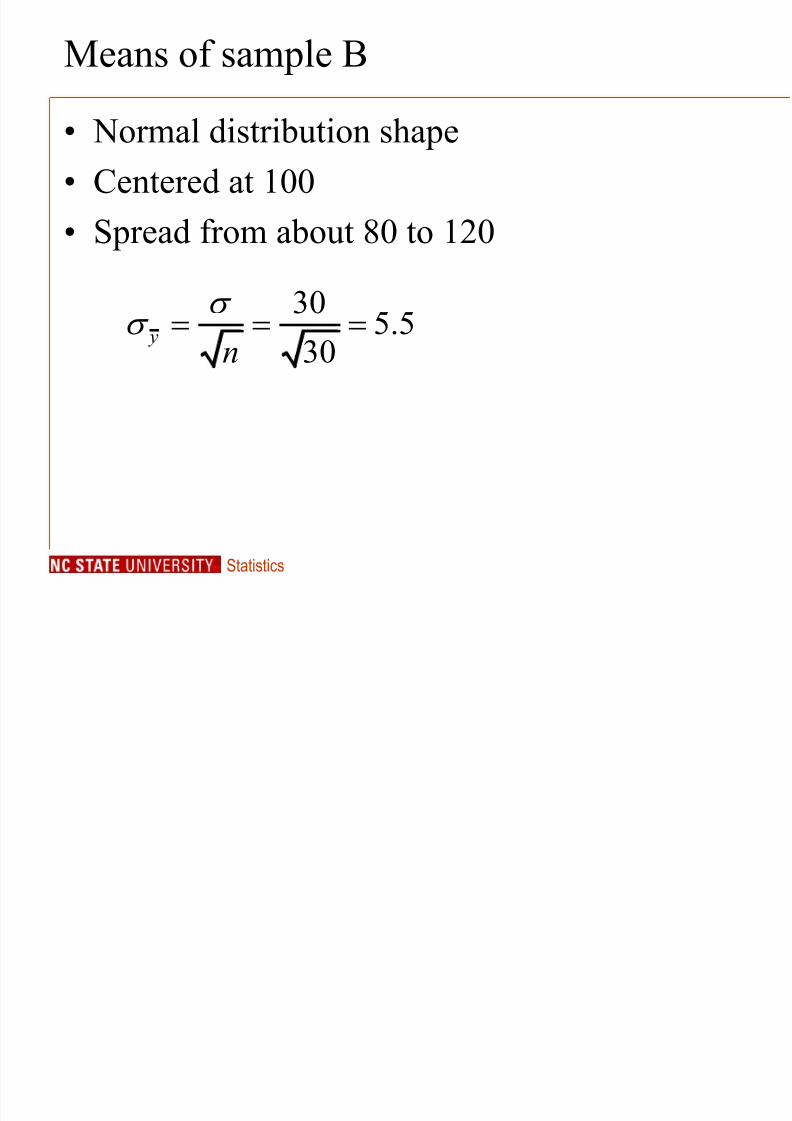
Means of sample B

• Normal distribution shape • Centered at 100 • Spread from about 80 to 120

305.5

30 y

n



Statistics

Differences



Statistics

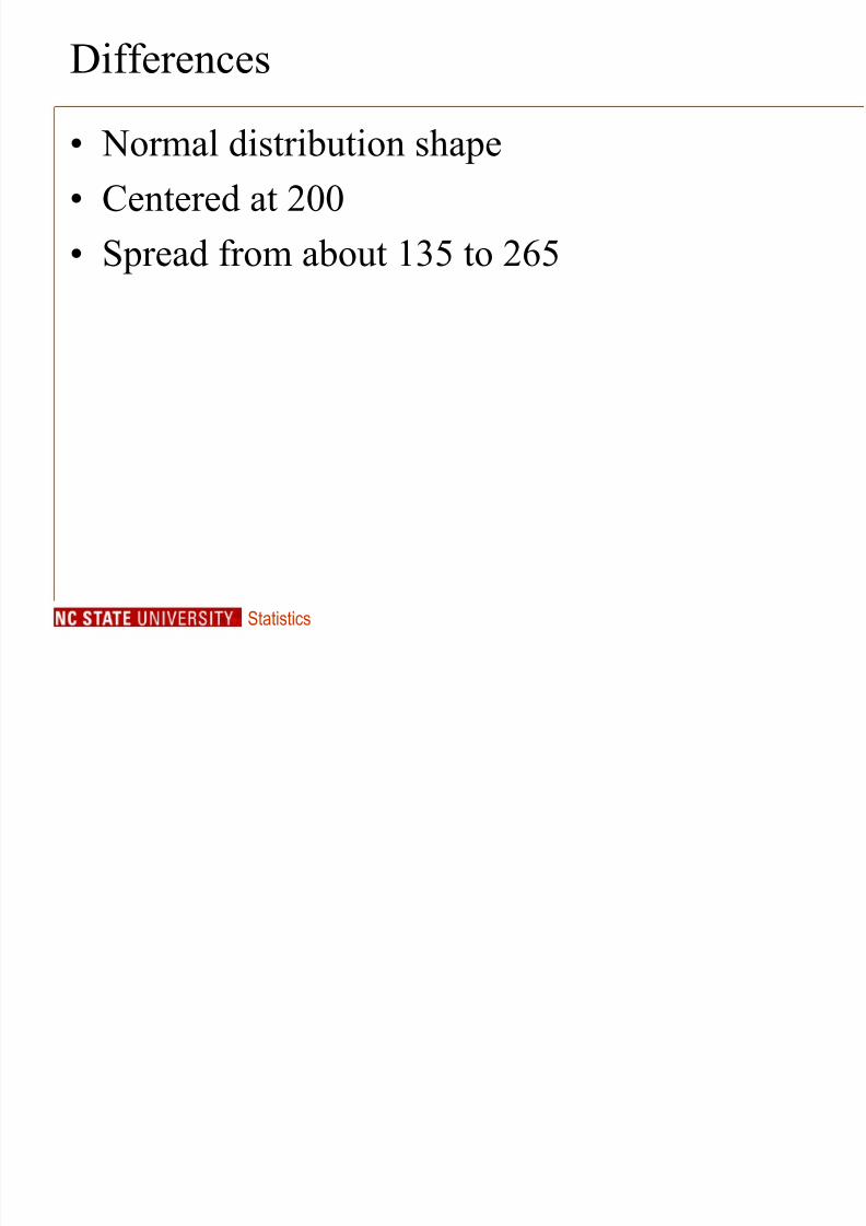
Differences

• Normal distribution shape • Centered at 200 • Spread from about 135 to 265



Statistics

Fact

• The difference in two independent normallydistributed variables will be normal. – Must know variables are independent



Statistics 15

Fact

• For independent random variables y 1 and y 2 the variance of the difference is the sum of thevariances

• Var(y 1- y2)=Var(y 1)+ Var(y 2)



Statistics 16

Some basic principles

• For independent random variables y 1 and y 2 the variance of the difference is the sum of thevariances

• Var(y 1- y2)=Var(y 1)+ Var(y 2)

• Note difference still gives sum!!



Statistics 17

Recall

1

2

1

1

2

2

y

y

n

n



Statistics 18

Recall

1 1

2 2

2

21 1

1 1

222 2

2 2

y y

y y

nn

nn

• Variance of sample mean



Statistics 19

Important formula

1 2

2 21 2

1 2 y y

n n



Statistics 20

Important formula

1 2

2 21 2

1 2 y y

n n

•

Standarderror ofdifferencein samplemeans



Statistics 21

Important formula

1 2

2 21 2

1 2 y y

n n

•

Standarderror ofdifferencein samplemeans

• Varianceof sampleone mean

• Varianceof sampletwo mean



Statistics

Note

• In most cases we will not know σ1 or σ2,instead we will substitute s 1 and s 2 (the sampleSD’s). This will not make a difference if thesamples are large.



Statistics

Test for difference in means: Two-sample ttest for independent samples

• Assumptions – Samples are random – Both populations are normally distributed.

– The samples are independent.



Statistics

Test for difference in means: Two-sample ttest for independent samples

• Assumptions – Samples are random – Both populations are normally distributed.

– The samples are independent.

• Needed to know distribution ofdifference



Statistics

Hypotheses

Null Hypothesis H0: 1- 2= 0 Alternative hypothesis

H1: 1- 2 > 0 H1: 1- 2 < 0 H1: 1- 2 0

Where 0 is some specific value (i.e., the null value)which is usually 0.



Statistics

Test Statistic

0

statistic-null valuestandard error t



Statistics

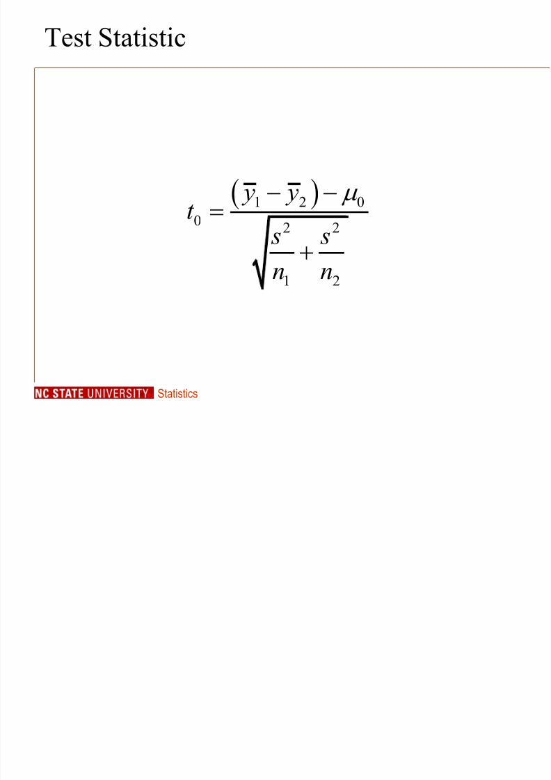
Test Statistic

1 2 00 2 2

1 2

1 2

y yt s sn n



Statistics

Test Statistic

1 2 00 2 2

1 2

1 2

y yt s sn n

• From nullhypothesis

• SampleMeans



Statistics

p-value

• t-distribution – Found from t-table

• Degrees of freedom

– We will use (n 1+n2-2) – approximately correct if the sample size is large – approximately correct if n 1=n 2 and s 1 =s2

– Use software in other situations to find exact df. • Found in direction of alternative hypothesis



Statistics

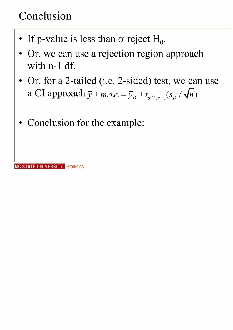
Conclusion

• If p-value is less than reject H 0.



Statistics

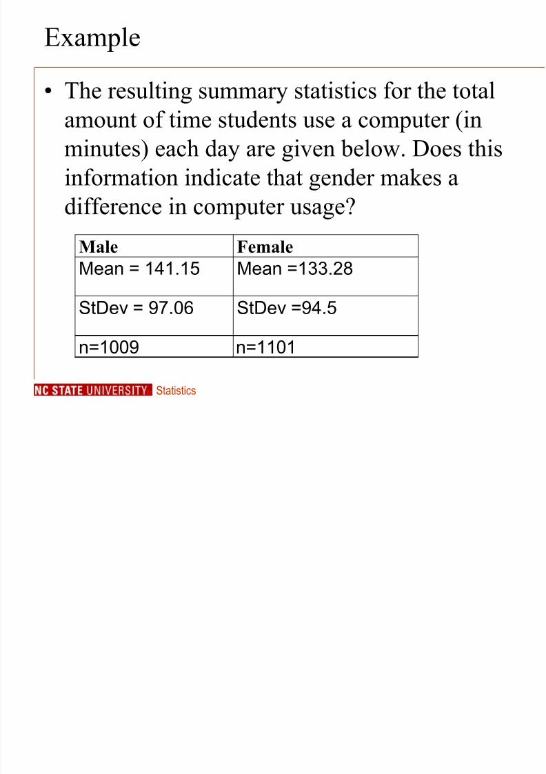
Example

• The resulting summary statistics for the totalamount of time students use a computer (inminutes) each day are given below. Does thisinformation indicate that gender makes adifference in computer usage?

Male FemaleMean = 141.15 Mean =133.28

StDev = 97.06 StDev =94.5

n=1009 n=1101



Statistics

Example

• Assumptions – Samples are random – Populations are normally distributed.

– The samples are independent.• H0: 1- 2= 0 (males and females are the

same in terms of computer usage) •

H1: 1- 2 0 (males and females differin terms of computer usage).



Statistics

Example

1 2 0

2 2 2 21 2

1 2

y - y - μ 141.15-133.28 -0t = =

s s 97.06 94.5++1009 1101n n

7.87 =1.8817.45



Statistics

Example

• P-value – See t-table – Degrees of freedom

– df = n 1+n 2-2=2108 – use last row on the table.



Statistics

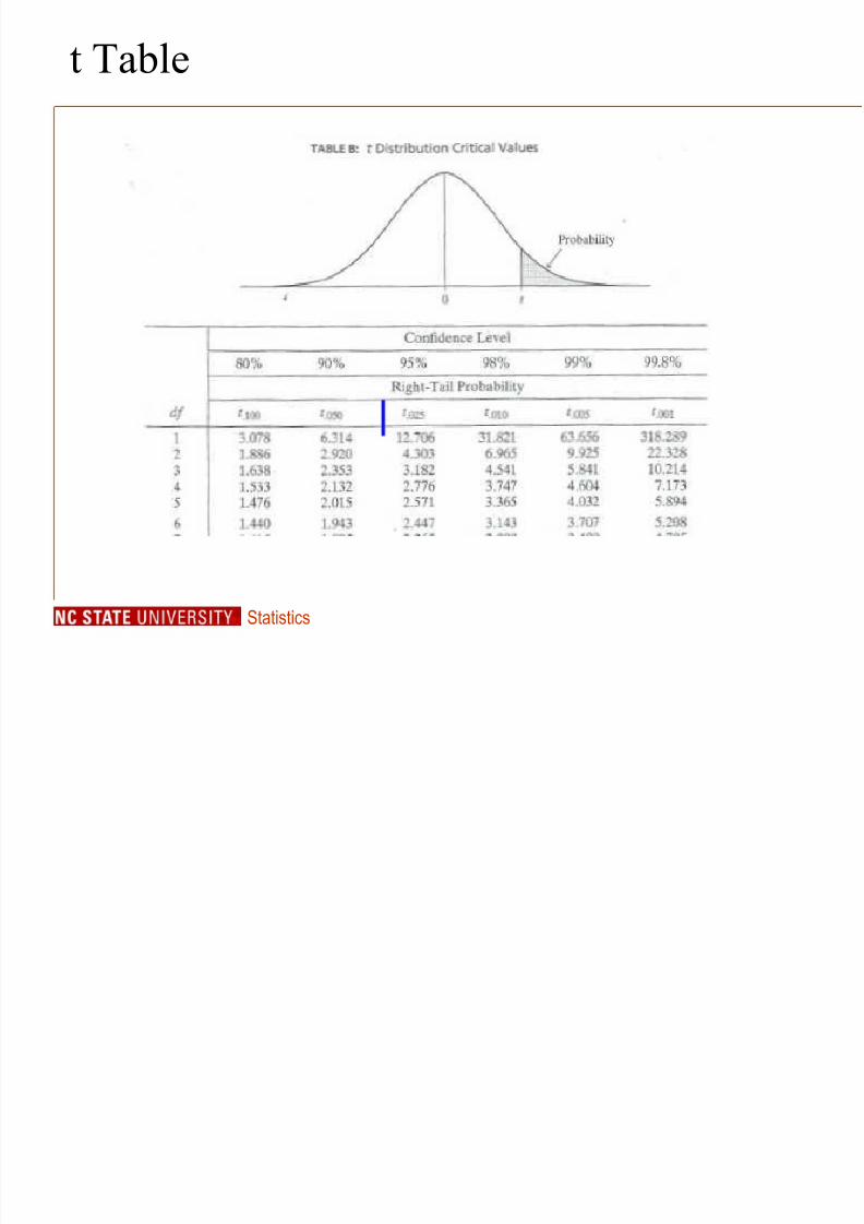
t Table

• 1.88 is between 1.645 and 1.96



Statistics

t Table



Statistics

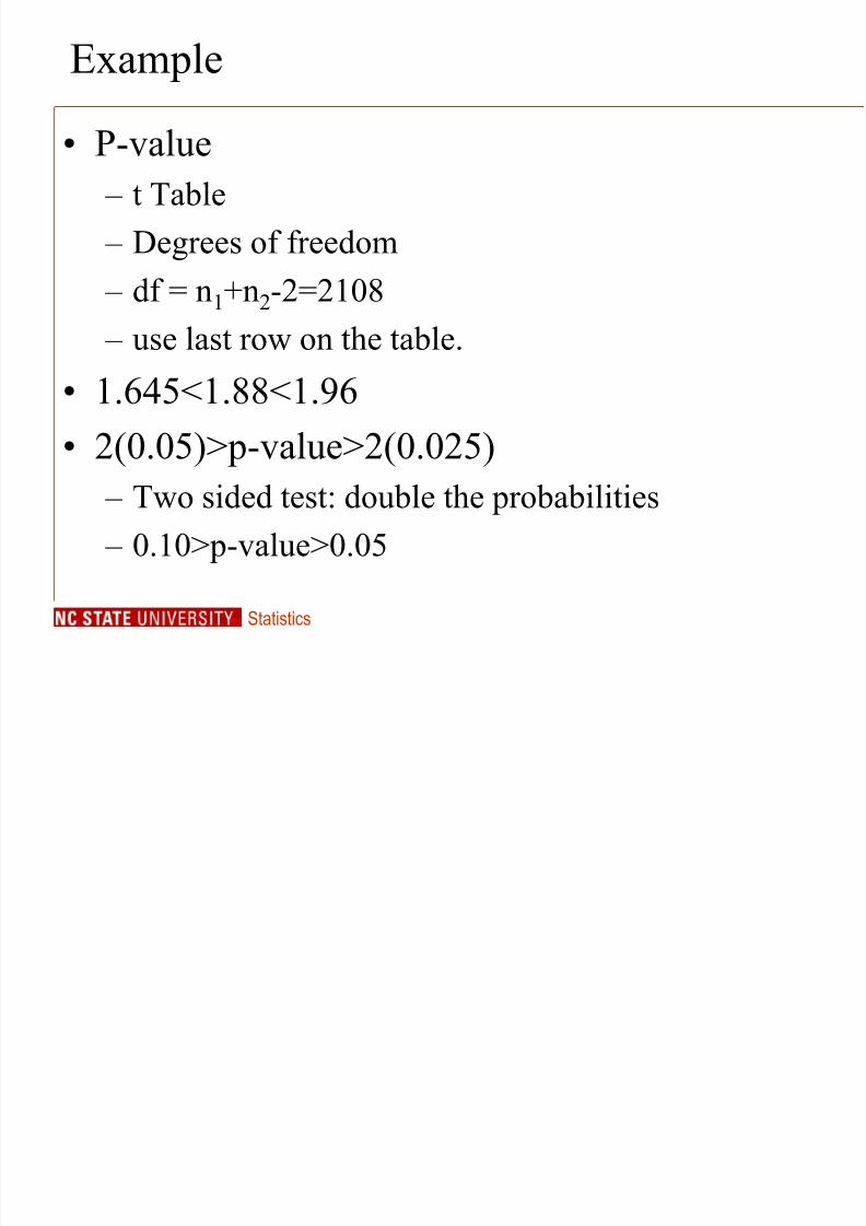
Example

• P-value – t Table – Degrees of freedom – df = n

1+n

2-2=2108

– use last row on the table.

• 1.645<1.88<1.96

• 2(0.05)>p-value>2(0.025) – Two sided test: double the probabilities – 0.10>p-value>0.05



Statistics

Example

• If p-value <= reject H 0.• p-value>0.05 Do not reject H0 • Not enough evidence to conclude that there is a

difference in computer usage between malesand females



Statistics

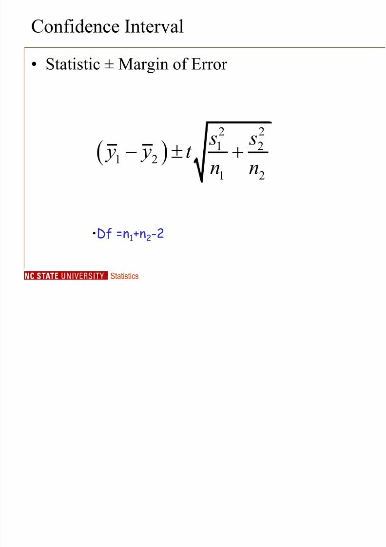
Confidence Interval

• Statistic ± Margin of Error

2 21 21 2

1 2

s s y y t n n



Statistics

Confidence Interval

• Statistic ± Margin of Error

2 21 21 2

1 2

s s y y t n n

• Df =n1+n2-2



Statistics

Example

• We would like to find a 95% confidenceinterval for the mean difference between maleand female computer usage in this population .

Male FemaleMean = 141.15 Mean =133.28

StDev = 97.06 StDev =94.5

n=1009 n=1101



Statistics

Example

2 21 21 2

1 2

2 2

s s y - y ± t +n n

97.06 94.5141.15-133.28 ±1.96 +1009 1101

7.87 ±1.96 17.45 => 7.87 ±8.19(-0.32,16.06)



Statistics

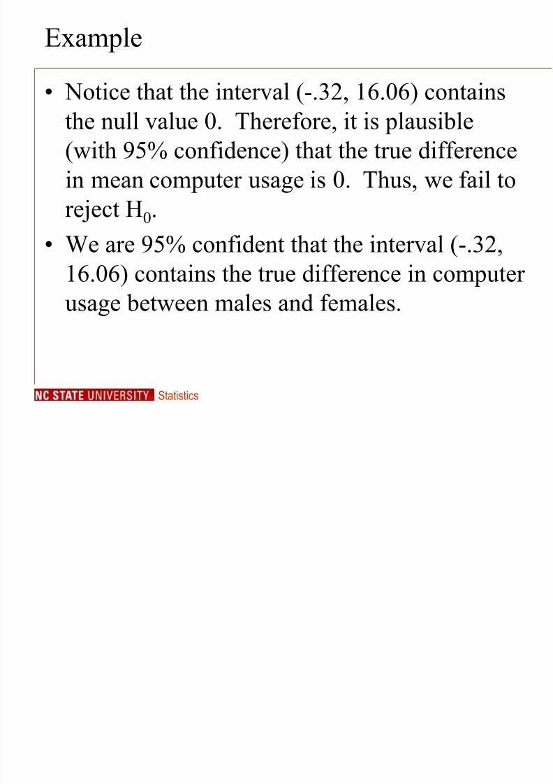
Example

• Notice that the interval (-.32, 16.06) containsthe null value 0. Therefore, it is plausible(with 95% confidence) that the true differencein mean computer usage is 0. Thus, we fail toreject H 0.

• We are 95% confident that the interval (-.32,16.06) contains the true difference in computer usage between males and females.



Statistics

General Rule: CI approach to a 2-tailed HT

• If the null value is contained in the 100(1- )%CI, then we FAIL TO REJECT H 0 at level .• If the null value is NOT contained in the

100(1- )% CI, then we REJECT H 0 at level .• Can only use this approach for a 2-tailed test



Statistics

Special Case: Pooled t-test

• In this section we take up a special case of thetwo sample t-test. – Used when we can make a specific assumption – Degrees of freedom will be exactly n

1+n

2-2

• Assume SD’s are equal: 1 = 2 – Pool the information you have about them.



Statistics

Pooled Variances

• Combine information about both variances intoa single estimate. Use this estimate in thestandard error formula.

2 21 1 2 22

1 2

1 1

2

n s n s s

n n

Test for difference in means



Statistics

Test for difference in means(pooled variance)

• Assumptions – Samples are random – Populations are normally distributed. – Population variances are equal. – Samples are independent.



Statistics

Hypotheses

Null Hypothesis H0: 1- 2= 0 Alternative hypothesis

H1: 1- 2 > 0 H1: 1- 2 < 0 H1: 1- 2 0

Where 0 is some specific (null) value.



Statistics

Test Statistic

1 2 00 2 2

1 2

y yt s sn n



Statistics

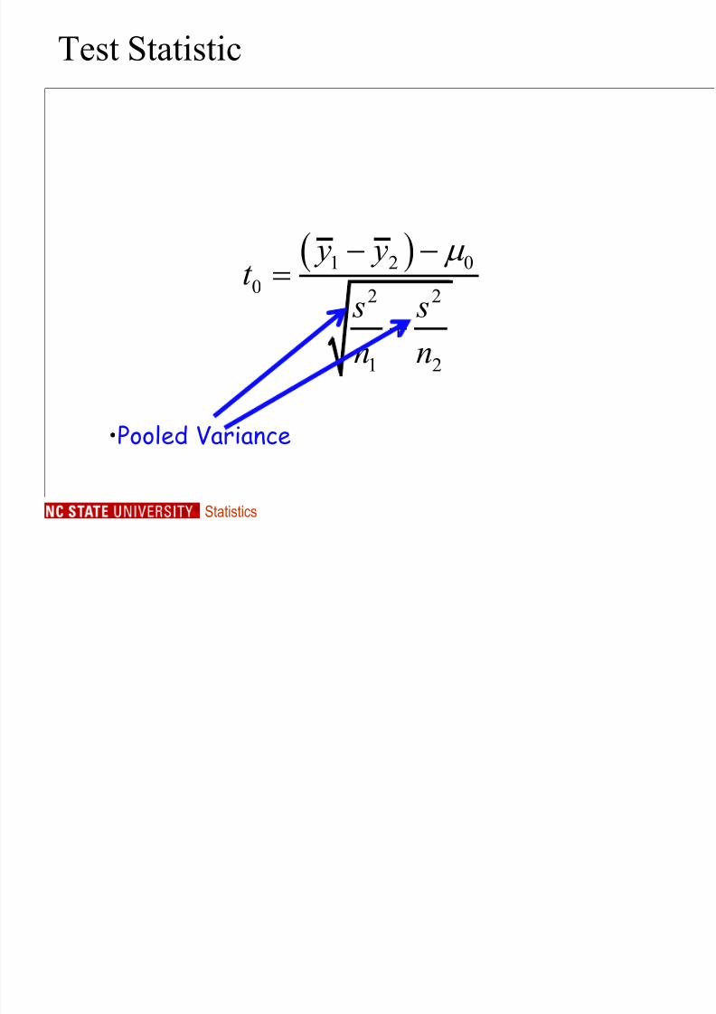
Test Statistic

1 2 00 2 2

1 2

y yt s sn n

• Pooled Variance



Statistics

p-value

• Found from t-table with n 1+n 2 – 2 degrees of freedom • Found in direction of alternative hypothesis

– For two sided ( ) alternative find one sided caseand double results.



Statistics

Conclusion

• If p-value <= reject H 0.



Statistics

Note: Can also use rejection region

• For both the “separate” and “pooled” variancetwo-sample t-test, we can also use a rejectionregion approach. Recall:

• Select a significance level .• Determine the Rejection Region: set of values

for which one rejects H 0.

• Compute the sample mean and the teststatistic. Reject H 0 if the test statistic lies inthe rejection region.



Statistics

Note: Can also use rejection region

• Alternative Hypothesis & Rejection Region

H 1 Rejection Region

H1: 1- 2 0 |t0 | > t /2, n1 n2 2

H1: 1- 2 > 0 t0 > t , n1 n2 2

H1: 1- 2 < 0 t0 < - t , n1 n2 2



Statistics

Example

• Does the color of paper make a difference inexam scores? A history professor created twoversions of an exam. The two versions were

printed on two colors of paper. Headministered them to his class by randomlyassigning them to his students.



Statistics

Example

• Twenty-one students took the exam versionthat was on pink paper. Eighteen studentswere assigned to the version on gold paper.The resulting scores are summarized below.Does this indicate that there is a significantdifference between the two colors of the exam?

Color n Mean St. DevPink 21 72 8.1

Gold 18 64 9.2



Statistics

Example

• Assumptions – Samples are random – Populations are normally distributed – Populations have same variance – The samples are independent.

• H0: 1- 2= 0 (version of the exam doesnot make a difference)

• H1: 1- 2 0 (versions do make adifference).



Statistics

Example

2 21 1 2 22

1 22 2

n -1 s + n -1 ss =n +n -2

21-1 8.1 + 18-1 9.2= 21+18-2

21-1 65.61+ 18-1 84.64=

21+18-21312.2+1438.88 2751.08= = 74.3537 37



Statistics

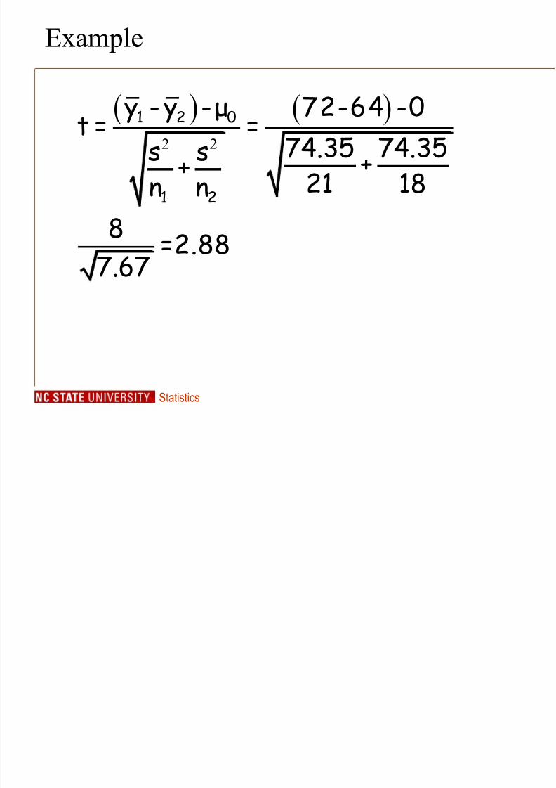
Example

2 2

1 2 0

1 2

y - y - μ 72-64 -0t = =74.35 74.35s s ++ 21 18

n n8 =2.887.67



Statistics

P-value

• Degrees of freedom • n1+n 2 – 2=21+18-2=37

• Closest df=38 (can round up or down) • 2*(0.005)>p-value • 0.010>p-value

l



Statistics

Conclusion.

• P-value is less than 0.05=> Reject H 0 • There is evidence of a significant difference

between the 2 versions of the exam.



E l



Statistics

Example

• Calculate a 95% confidence interval for thedifference in mean score of exams for the twoversions. – 37 degrees of freedom

E l



Statistics

Example

2 2

1 21 2

s s y - y ± t +n n

74.35 74.358±2.024 +21 18

8±2.024 7.67 => 8±5.605(2.4,13.6)

E l



Statistics

Example

• Notice that the null value “0” is not containedin the interval (2.4, 13.6), so we reject the nullhypothesis.

• We are 95% confident that the interval (2.4,13.6) contains the true mean difference

between the exam versions. OR • The observed interval (2.4, 13.6) brackets the

true difference in mean exam scores, with 95%confidence.

Wh d d hi ?



Statistics

When do we do this test?

• For any sample size (especially when n issmall) and• If we can make the assumption of equal

variances – Often ok if we have two randomly assigned groups

• When using software distinction not asimportant. – Was more important before computing – Probably see this test in literature.

P i d Diff



Statistics

Paired Differences

• Compare two measures on the same subject – Right and left hand – Pre-test and post-test – Before and after measure

• Record two measures on same subject – Take the difference in those measures – Change scores

E l



Statistics

Example

• We recorded the right and left hand strength of 9randomly selected college age adults.

E l



Statistics

Example

Subject Dominant Off Dom1 333 3502 380 3743 164 1894 330 308

5 214 2096 282 2247 390 3828 258 2939 221 219

E l



Statistics

Example

Subject Dominant Off Dom Difference1 333 350 -172 380 374 63 164 189 -254 330 308 225 214 209 56 282 224 587 390 382 88 258 293 -359 221 219 2

E l



Statistics

Example

• Treat differences as a single sample

• Hypotheses:

– If there is no difference average should be 0 – If dominant hand is stronger difference should be

greater than 0

Notation



Statistics

Notation

D

sample average of differences

s standard deviation of differences

n number of differences

D y

Example



Statistics

Example

D

D

y = ______ s =27.50n = _______

Test for paired differences



Statistics

Test for paired differences

• Assumption – We have a random sample of the differences – The population of differences is normally

distributed.

Hypotheses



Statistics

Hypotheses

H0: =

0

H1: > 0

H1: < 0 H1: 0

Where is really D, the true mean of thedifferences

Test Statistic



Statistics

Test Statistic

00

D

D

yt s

n

Test Statistic



Statistics

Test Statistic

00

D

D yt s

n

From nullhypothesis

(usually zero)

Mean of sample

SD of sample

Test Statistic: Example



Statistics

Test Statistic: Example

00 ? D

D

yt s

n

p value



Statistics

p-value

• Found from t-table using n-1 degrees of freedom.



Rejection Region Approach



Statistics

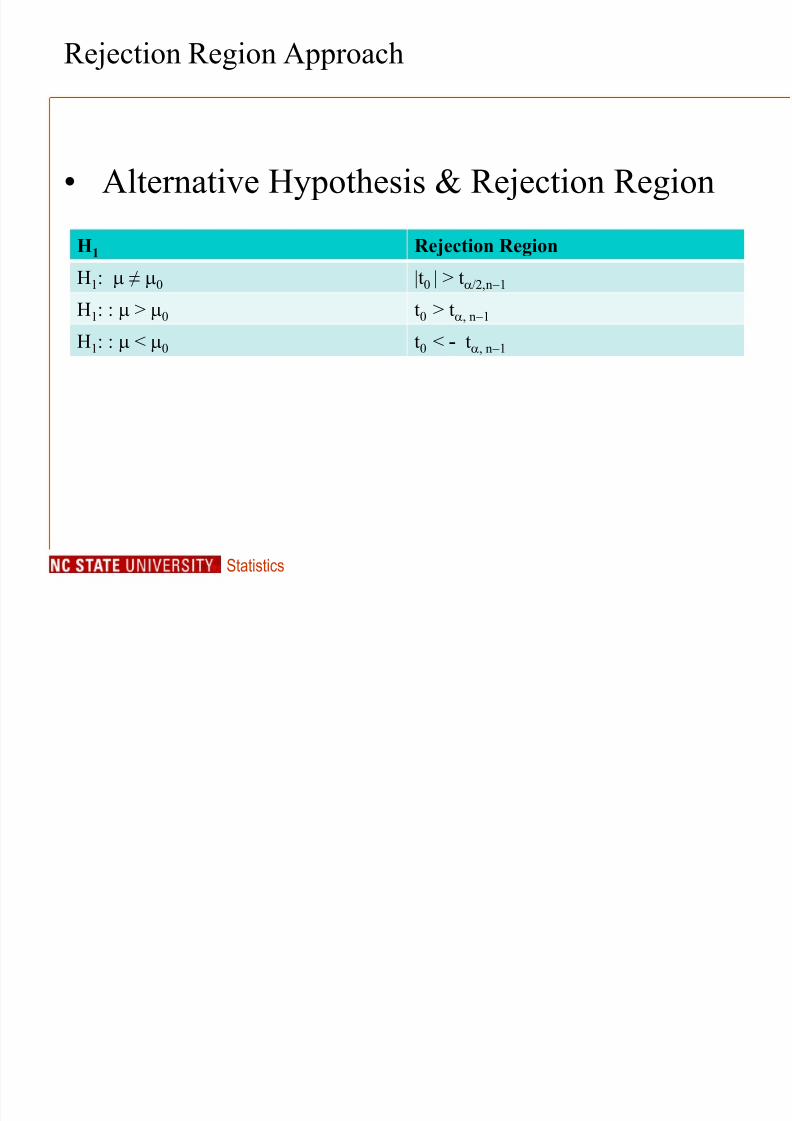
Rejection Region Approach

• Alternative Hypothesis & Rejection Region

H 1 Rejection Region

H1: ≠

0|t

0| > t

/2, n 1H1: : > 0 t0 > t , n 1

H1: : < 0 t0 < - t , n 1

CI for the mean µ of a normal distribution, when σ is



Statistics

unknown (cont’d)

• When σ is unknown, the (1- α)% CI for µ for a particular

sample (x1 ,…, xn ) is:

where is the sample mean, s is the sample standarddeviation, n is the sample size, is the critical value of a

t distribution with df=n-1 corresponding to a right tail probability of α/2.

/2, 1. . . /n x m o e x t x n

x/2, 1nt

Example: Twin Weights



Example: Twin Weights

• http://www.statcrunch.com/5.0/index.php?dataid=338704 • Weights for 19 newborn twins born to members of the Greater

Columbia South Carolina Area Mothers of Twins Club fromSeptember 2000 to December 2001.

http://www.statcrunch.com/5.0/index.php?dataid=338704

http://www.statcrunch.com/5.0/index.php?dataid=338704

lecture 14. ht and ci for two means (2)

Documents