lecture 14 value of information - college of engineeringlecture 14 value of information jitesh h....

Introduction to Value of InformationExpected Value of Perfect Information

Expected Value of Imperfect Information

Lecture 14Value of Information

Jitesh H. Panchal

ME 597: Decision Making for Engineering Systems Design

Design Engineering Lab @ Purdue (DELP)School of Mechanical Engineering

Purdue University, West Lafayette, INhttp://engineering.purdue.edu/delp

October 10, 2019ME 597: Fall 2019 Lecture 14 1 / 29

http://engineering.purdue.edu/delp



Lecture Outline

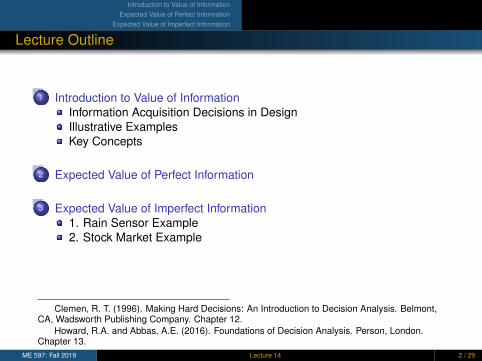
1 Introduction to Value of InformationInformation Acquisition Decisions in DesignIllustrative ExamplesKey Concepts

2 Expected Value of Perfect Information

3 Expected Value of Imperfect Information1. Rain Sensor Example2. Stock Market Example

Clemen, R. T. (1996). Making Hard Decisions: An Introduction to Decision Analysis. Belmont,CA, Wadsworth Publishing Company. Chapter 12.

Howard, R.A. and Abbas, A.E. (2016). Foundations of Decision Analysis. Person, London.Chapter 13.

ME 597: Fall 2019 Lecture 14 2 / 29



Information Acquisition Decisions in DesignIllustrative ExamplesKey Concepts

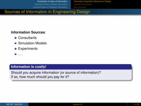
Sources of Information in Engineering Design

Information Sources:

Consultants

Simulation Models

Experiments

. . .

Information is costly!

Should you acquire information (or source of information)?If so, how much should you pay for it?

ME 597: Fall 2019 Lecture 14 3 / 29




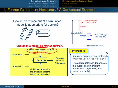
Is Further Refinement Necessary? A Conceptual Example

How much refinement of a simulation

model is appropriate for design?

R

R LR L

T

Material Alternatives

Decision

Material 1

Simulation model predicts

material strength

Objective: Maximize

the pressure that the

vessel can withstand

Selected

Material

Alternative

Material 2

Should this model be refined further?

• Improved accuracy does not imply

improved usefulness in design !!!

• The appropriateness depends on

the overall design problem

(constraints, objectives, and

variable bounds)

Inferences

Material 1

Material 2Predicted Strength

Predicted Strength

Strength (MPa)

[150 175] MPa

[190 225] MPa

ME 597: Fall 2019 Lecture 14 4 / 29




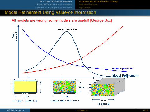
Model Refinement Using Value-of-Information

All models are wrong, some models are useful! [George Box]

ME 597: Fall 2019 Lecture 14 5 / 29




Basic Questions

Questions to be addressed:

What is an appropriate basis on which to evaluate the value ofinformation in a decision situation?

What does it mean for an expert to provide perfect information?

How does probability relate to the idea of information?

ME 597: Fall 2019 Lecture 14 6 / 29




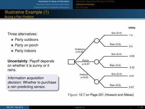
Illustrative Example (1)Buying a Rain Predictor

Three alternatives:

Party outdoors

Party on porch

Party indoors

Uncertainty: Payoff dependson whether it is sunny or itrains.

Information acquisitiondecision: Whether to purchasea rain predicting sensor.

Sun (0.4)

Rain (0.6)

Indoors

Porch

1.0

0.0Outdoors

Utility

Sun (0.4)

Rain (0.6)

Sun (0.4)

Rain (0.6)

0.32

0.67

0.95

0.57

u=0.40

u=0.57

u=0.63

Figure: 10.7 on Page 201 (Howard and Abbas)

ME 597: Fall 2019 Lecture 14 7 / 29




Illustrative Example (2)Investing in the Stock Market

Investor has three alternatives:

High-risk stock

Low-risk stock

Savings account

Uncertainty: Payoff on stocksdepends on whether themarket goes up, remainssame, or goes down.

Information acquisitiondecision: Whether to getexpert advice.

Savings account

Up (0.5)

Same (0.3)

Down (0.2)

High-Risk

Stock

Low-Risk

Stock

Up (0.5)

Same (0.3)

Down (0.2)

1500

100

-1000

1000

200

-100

500

Figure: 12.1 on Page 436 (Clemen)

ME 597: Fall 2019 Lecture 14 8 / 29




The Expected Value of Information – Key Concepts (1)

If the decision maker will make the same decision regardless of what the newinformation is, then the information has no value!

Rain Prediction Sensor Example:

The best decision without the sensor is to hold the party indoors.

If after buying the sensor, the decision still remains the same(irrespective of what the sensor shows) ⇒ no value.

ME 597: Fall 2019 Lecture 14 9 / 29




The Expected Value of Information – Key Concepts (2)

Value of information needs to be determined before actually getting theinformation (e.g., before hiring the expert).

Worst case scenario: Decision remains the same even after hiring theexpert ⇒ Zero value of information.

Better scenarios: Expected value increases ⇒ Positive value ofinformation.

Best case scenario: Perfect Information (resolving all uncertainty; Experttells us exactly what will happen) ⇒ Maximum value of information (i.e.,Expected Value of Perfect Information).

ME 597: Fall 2019 Lecture 14 10 / 29



The Notion of “Perfect Information”

Clairvoyant: An expert’s information is said to be perfect if it is alwayscorrect.

1 When state S will occur, the information source always says so.The sensor accurately states whether it will rain or not, i.e.,P(Sensor predicts ”Sunshine” | Weather will actually be Sunny) = 1In the stock market example,P(Expert says “Market Up” | Market really Does Go Up) = 1

2 Also, the expert must never say that the state S will occur if any otherstate (S̄) will occur.

ME 597: Fall 2019 Lecture 14 11 / 29



Decision Tree without Additional Information

Decision maker’s prior probabilities: Sun (0.4) and Rain (0.6).

Sun (0.4)

Rain (0.6)

Indoors

Porch

1.0

0.0Outdoors

Utility

Sun (0.4)

Rain (0.6)

Sun (0.4)

Rain (0.6)

0.32

0.67

0.95

0.57

u=0.40

u=0.57

u=0.63


ME 597: Fall 2019 Lecture 14 12 / 29



Decision Tree with Clairvoyance


ME 597: Fall 2019 Lecture 14 13 / 29



1. Rain Sensor Example2. Stock Market Example

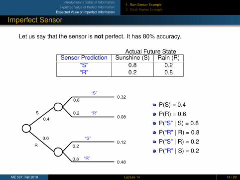
Imperfect Sensor

Let us say that the sensor is not perfect. It has 80% accuracy.

Actual Future StateSensor Prediction Sunshine (S) Rain (R)

“S” 0.8 0.2“R” 0.2 0.8

“S”

“R”

0.32

0.08

“S”

“R”

0.12

0.48

S

R

0.4

0.6

0.8

0.2

0.2

0.8

P(S) = 0.4

P(R) = 0.6

P(“S” | S) = 0.8

P(“R” | R) = 0.8

P(“S” | R) = 0.2

P(“R” | S) = 0.2

ME 597: Fall 2019 Lecture 14 14 / 29




Uncertainties When Using the Sensor

S

R

P(“S”, S)=?

P(“S”, R)=?

S

R

P(“R”, S)=?

P(“R”, R)=?

“S”

“R”

P(“S”) = ?

P(“R”) = ?

P(S|“S”)=?

P(R|“S”)=?

P(S|“R”)=?

P(R|“R”)=?

Sensor Prediction

Future State

ME 597: Fall 2019 Lecture 14 15 / 29




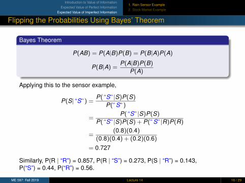
Flipping the Probabilities Using Bayes’ Theorem

S

R

P(“S”,uS)=0.32

P(“S”,uR)=0.12

S

R

P(“R”,uS)=0.08

P(“R”,uR)=0.48

“S”

“R”

P(“S”)u=u0.44

P(“R”)u=u0.56

P(S|“S”)=0.727

P(R|“S”)=0.273

P(S|“R”)=0.143

P(R|“R”)=0.857

SensoruPrediction

FutureuState

ME 597: Fall 2019 Lecture 14 17 / 29




Including Decisions in the Tree

ME 597: Fall 2019 Lecture 14 18 / 29




Illustrative Example (2)Investing in the Stock Market

Investor has three alternatives:

High-risk stock

Low-risk stock

Savings account

Uncertainty: Payoff on stocksdepends on whether themarket goes up, remainssame, or goes down.

Information acquisitiondecision: Whether to getexpert advice.

Savings account

Up (0.5)

Same (0.3)

Down (0.2)

High-Risk

Stock

Low-Risk

Stock

Up (0.5)

Same (0.3)

Down (0.2)

1500

100

-1000

1000

200

-100

500


ME 597: Fall 2019 Lecture 14 19 / 29




Example of Stock Market InvestmentDeciding whether to hire the clairvoyant consultant

The decision maker has not yet consulted the clairvoyant. He is consideringwhether or not to consult!

There is 50% chance that the clairvoyant would say that the market will goup, 30% chance that the market will stay flat, and 20% chance that themarket will go down.

ME 597: Fall 2019 Lecture 14 20 / 29




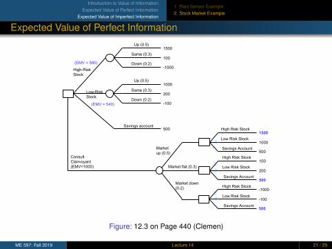
Expected Value of Perfect Information

Market

up (0.5)

Up (0.5)

Same (0.3)

Down (0.2)

High-Risk

Stock

Low-Risk

Stock

Up (0.5)

Same (0.3)

Down (0.2)

1500

100

-1000

1000

200

-100

500

(EMV = 540)

(EMV = 580)

High Risk Stock

Low Risk Stock

Savings Account

1500

1000

500

100

200

500

-1000

-100

500

Savings account

Market down

(0.2)

Market flat (0.3)

Consult

Clairvoyant

(EMV=1000)

High Risk Stock

Low Risk Stock

Savings Account

High Risk Stock

Low Risk Stock

Savings Account


ME 597: Fall 2019 Lecture 14 21 / 29




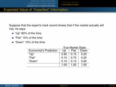
Expected Value of “Imperfect” Information

Suppose that the expert’s track record shows that if the market actually willrise, he says:

“Up” 80% of the time

“Flat” 10% of the time

“Down” 10% of the time

True Market StateEconomist’s Prediction Up Flat Down“Up” 0.80 0.15 0.20“Flat” 0.10 0.70 0.20“Down” 0.10 0.15 0.60

1.00 1.00 1.00

ME 597: Fall 2019 Lecture 14 22 / 29




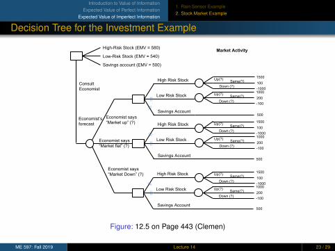
Decision Tree for the Investment Example

Economist says

“Market up” (?)

High-Risk Stock (EMV = 580)

Low-Risk Stock (EMV = 540)

High Risk Stock

Low Risk Stock

Savings Account

Savings account (EMV = 500)

Economist’s

forecast

Economist says

“Market flat” (?)

Economist says

“Market Down” (?) High Risk Stock

Low Risk Stock

Savings Account

High Risk Stock

Low Risk Stock

Savings Account

500

Down (?)

Up(?)Same(?)

1000

200

-100

Market Activity

Down (?)

Up(?)Same(?)

1500

100

-1000

Down (?)

Up(?)Same(?)

1500

100

-1000

Down (?)

Up(?)Same(?)

1000

200

-100

Down (?)

Up(?)Same(?)

1500

100

-1000

Down (?)

Up(?)Same(?)

1000

200

-100

500

500

Consult

Economist


ME 597: Fall 2019 Lecture 14 23 / 29




Flipping the Probability Tree

“Market up” (0.80)

Market up

(0.5)

Market

Flat (0.3)

Market

Down

(0.2)

Actual Market

Performance

Economist’s

Forecast

“Market Flat” (0.10)

“Market Down” (0.10)







Market up (?)

“Market

up” (?)

“Market

Flat” (?)

“Market

Down” (?)

Economist’s

Forecast

Actual Market

Performance

Market Flat (?)

Market Down (?)

Market up (?)

Market Flat (?)

Market Down (?)

Market up (?)

Market Flat (?)

Market Down (?)


ME 597: Fall 2019 Lecture 14 24 / 29




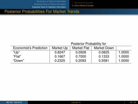
Posterior Probabilities For Market Trends

Posterior Probability forEconomist’s Prediction Market Up Market Flat Market Down“Up” 0.8247 0.0928 0.0825 1.0000“Flat” 0.1667 0.7000 0.1333 1.0000“Down” 0.2325 0.2093 0.5581 1.0000

ME 597: Fall 2019 Lecture 14 26 / 29




Completed Decision Tree

Economist says

“Market up”

(0.485)

High-Risk Stock (EMV = 580)

Low-Risk Stock (EMV = 540)

High Risk Stock

Low Risk Stock

Savings Account

Savings account (EMV = 500)

Economist’s

forecast

Economist says

“Market flat”

(0.300)

Economist says

“Market Down”

(0.215)

High Risk Stock

Low Risk Stock

Savings Account

High Risk Stock

Low Risk Stock

Savings Account

500

Down (0.0825)

Up(0.8247)Same(0.0928)

1000

200

-100

Down (0.0825)

Up(0.8247)Same(0.0928)

1500

100

-1000

Down (0.1333)

Up(0.1667)Same(0.7000)

1500

100

-1000

Down (0.1333)

Up (0.1667)Same(0.7000)

1000

200

-100

Down (0.5581)

Up(0.2325)Same(0.2093)

1500

100

-1000

Down (0.5581)

Up(0.2325)Same(0.2093)

1000

200

-100

500

500

Consult

Economist

(EMV=822)

EMV=1164

EMV=835

EMV=187

EMV=293

EMV=-188

EMV=219


ME 597: Fall 2019 Lecture 14 27 / 29




Summary

1 Introduction to Value of InformationInformation Acquisition Decisions in DesignIllustrative ExamplesKey Concepts

2 Expected Value of Perfect Information

3 Expected Value of Imperfect Information1. Rain Sensor Example2. Stock Market Example

Clemen, R. T. (1996). Making Hard Decisions: An Introduction to Decision Analysis. Belmont,CA, Wadsworth Publishing Company. Chapter 12.

Howard, R.A. and Abbas, A.E. (2016). Foundations of Decision Analysis. Person, London.Chapter 13.

ME 597: Fall 2019 Lecture 14 28 / 29




References

1 Clemen, R. T. (1996). Making Hard Decisions: An Introduction toDecision Analysis. Belmont, CA, Wadsworth Publishing Company.Chapter 12.

2 Howard, R.A. and Abbas, A.E. (2016). Foundations of Decision Analysis.Person, London. Chapter 13.

ME 597: Fall 2019 Lecture 14 29 / 29

lecture 14 value of information - college of engineeringlecture 14 value of information jitesh h....

Documents