lecture 2 sequence alignment and dynamic programming · sequence alignment and dynamic programming...

Lecture 2

Sequence Alignment and Dynamic Programming

6.047/6.878/HST.507 Computational Biology: Genomes, Networks, Evolution

1

Module 1: Aligning and modeling genomes

• Module 1: Computational foundations – Dynamic programming: exploring exponential spaces in poly-time – Introduce Hidden Markov Models (HMMs): Central tool in CS – HMM algorithms: Decoding, evaluation, parsing, likelihood, scoring

• This week: Sequence alignment / comparative genomics – Local/global alignment: infer nucleotide-level evolutionary events – Database search: scan for regions that may have common ancestry

• Next week: Modeling genomes / exon / CpG island finding – Modeling class of elements, recognizing members of a class – Application to gene finding, conservation islands, CpG islands

2

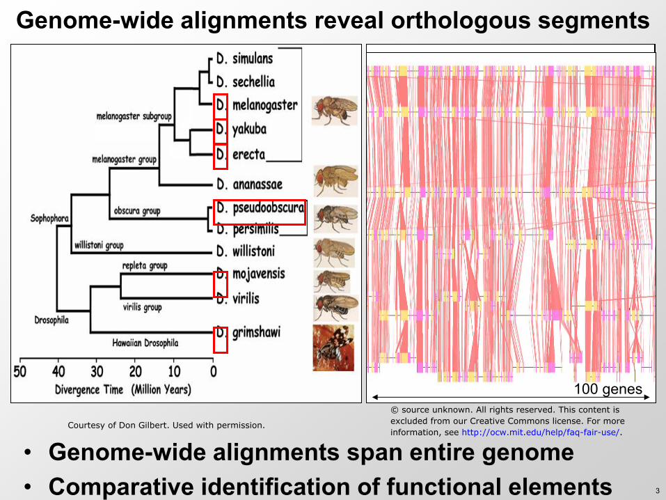
Genome-wide alignments reveal orthologous segments

• Genome-wide alignments span entire genome • Comparative identification of functional elements

100 genes

Courtesy of Don Gilbert. Used with permission.

3

© source unknown. All rights reserved. This content isexcluded from our Creative Commons license. For moreinformation, see http://ocw.mit.edu/help/faq-fair-use/.

http://ocw.mit.edu/help/faq-fair-use/

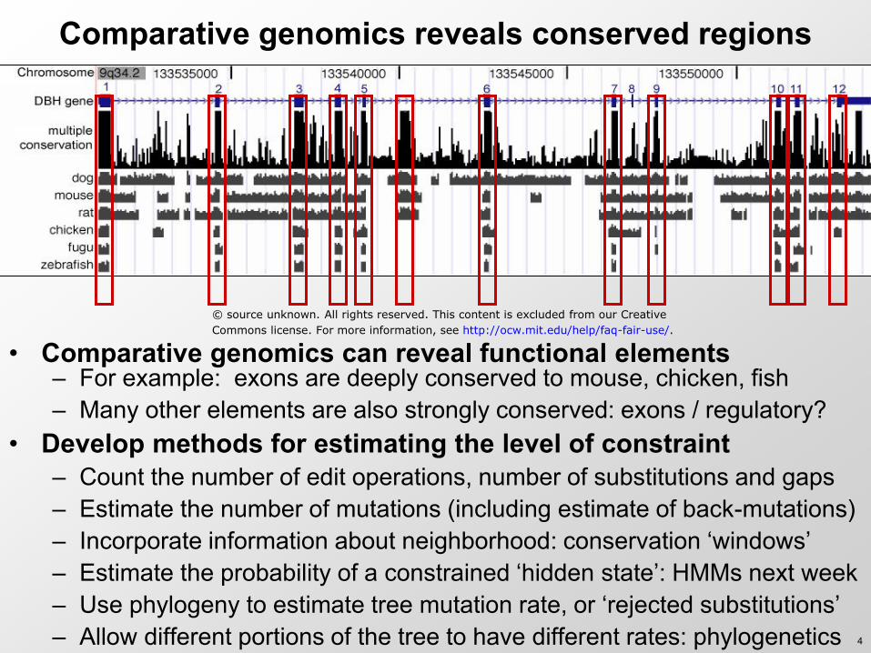
Comparative genomics reveals conserved regions

• Comparative genomics can reveal functional elements – For example: exons are deeply conserved to mouse, chicken, fish – Many other elements are also strongly conserved: exons / regulatory?

• Develop methods for estimating the level of constraint – Count the number of edit operations, number of substitutions and gaps – Estimate the number of mutations (including estimate of back-mutations) – Incorporate information about neighborhood: conservation ‘windows’ – Estimate the probability of a constrained ‘hidden state’: HMMs next week – Use phylogeny to estimate tree mutation rate, or ‘rejected substitutions’ – Allow different portions of the tree to have different rates: phylogenetics

© source unknown. All rights reserved. This content is excluded from our Creative

Commons license. For more information, see http://ocw.mit.edu/help/faq-fair-use/.

4


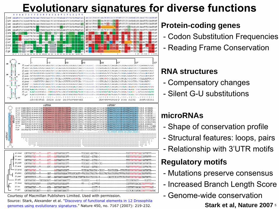
Evolutionary signatures for diverse functions Protein-coding genes

- Codon Substitution Frequencies - Reading Frame Conservation

RNA structures

- Compensatory changes - Silent G-U substitutions

microRNAs

- Shape of conservation profile - Structural features: loops, pairs - Relationship with 3’UTR motifs

Regulatory motifs

- Mutations preserve consensus - Increased Branch Length Score - Genome-wide conservation

Stark et al, Nature 2007

Courtesy of Macmillan Publishers Limited. Used with permission.

Source: Stark, Alexander et al. "Discovery of functional elements in 12 Drosophila

genomes using evolutionary signatures." Nature 450, no. 7167 (2007): 219-232. 5

10.1038/nature06340

10.1038/nature06340

Alignment: Evolution preserves functional elements!

Scer TTATATTGAATTTTCAAAAATTCTTACTTTTTTTTTGGATGGACGCAAAGAAGTTTAATAATCATATTACATGGCATTACCACCATATACA Spar CTATGTTGATCTTTTCAGAATTTTT-CACTATATTAAGATGGGTGCAAAGAAGTGTGATTATTATATTACATCGCTTTCCTATCATACACA Smik GTATATTGAATTTTTCAGTTTTTTTTCACTATCTTCAAGGTTATGTAAAAAA-TGTCAAGATAATATTACATTTCGTTACTATCATACACA Sbay TTTTTTTGATTTCTTTAGTTTTCTTTCTTTAACTTCAAAATTATAAAAGAAAGTGTAGTCACATCATGCTATCT-GTCACTATCACATATA * * **** * * * ** ** * * ** ** ** * * * ** ** * * * ** * * * Scer TATCCATATCTAATCTTACTTATATGTTGT-GGAAAT-GTAAAGAGCCCCATTATCTTAGCCTAAAAAAACC--TTCTCTTTGGAACTTTCAGTAATACG Spar TATCCATATCTAGTCTTACTTATATGTTGT-GAGAGT-GTTGATAACCCCAGTATCTTAACCCAAGAAAGCC--TT-TCTATGAAACTTGAACTG-TACG Smik TACCGATGTCTAGTCTTACTTATATGTTAC-GGGAATTGTTGGTAATCCCAGTCTCCCAGATCAAAAAAGGT--CTTTCTATGGAGCTTTG-CTA-TATG Sbay TAGATATTTCTGATCTTTCTTATATATTATAGAGAGATGCCAATAAACGTGCTACCTCGAACAAAAGAAGGGGATTTTCTGTAGGGCTTTCCCTATTTTG ** ** *** **** ******* ** * * * * * * * ** ** * *** * *** * * * Scer CTTAACTGCTCATTGC-----TATATTGAAGTACGGATTAGAAGCCGCCGAGCGGGCGACAGCCCTCCGACGGAAGACTCTCCTCCGTGCGTCCTCGTCT Spar CTAAACTGCTCATTGC-----AATATTGAAGTACGGATCAGAAGCCGCCGAGCGGACGACAGCCCTCCGACGGAATATTCCCCTCCGTGCGTCGCCGTCT Smik TTTAGCTGTTCAAG--------ATATTGAAATACGGATGAGAAGCCGCCGAACGGACGACAATTCCCCGACGGAACATTCTCCTCCGCGCGGCGTCCTCT Sbay TCTTATTGTCCATTACTTCGCAATGTTGAAATACGGATCAGAAGCTGCCGACCGGATGACAGTACTCCGGCGGAAAACTGTCCTCCGTGCGAAGTCGTCT ** ** ** ***** ******* ****** ***** *** **** * *** ***** * * ****** *** * *** Scer TCACCGG-TCGCGTTCCTGAAACGCAGATGTGCCTCGCGCCGCACTGCTCCGAACAATAAAGATTCTACAA-----TACTAGCTTTT--ATGGTTATGAA Spar TCGTCGGGTTGTGTCCCTTAA-CATCGATGTACCTCGCGCCGCCCTGCTCCGAACAATAAGGATTCTACAAGAAA-TACTTGTTTTTTTATGGTTATGAC Smik ACGTTGG-TCGCGTCCCTGAA-CATAGGTACGGCTCGCACCACCGTGGTCCGAACTATAATACTGGCATAAAGAGGTACTAATTTCT--ACGGTGATGCC Sbay GTG-CGGATCACGTCCCTGAT-TACTGAAGCGTCTCGCCCCGCCATACCCCGAACAATGCAAATGCAAGAACAAA-TGCCTGTAGTG--GCAGTTATGGT ** * ** *** * * ***** ** * * ****** ** * * ** * * ** *** Scer GAGGA-AAAATTGGCAGTAA----CCTGGCCCCACAAACCTT-CAAATTAACGAATCAAATTAACAACCATA-GGATGATAATGCGA------TTAG--T Spar AGGAACAAAATAAGCAGCCC----ACTGACCCCATATACCTTTCAAACTATTGAATCAAATTGGCCAGCATA-TGGTAATAGTACAG------TTAG--G Smik CAACGCAAAATAAACAGTCC----CCCGGCCCCACATACCTT-CAAATCGATGCGTAAAACTGGCTAGCATA-GAATTTTGGTAGCAA-AATATTAG--G Sbay GAACGTGAAATGACAATTCCTTGCCCCT-CCCCAATATACTTTGTTCCGTGTACAGCACACTGGATAGAACAATGATGGGGTTGCGGTCAAGCCTACTCG **** * * ***** *** * * * * * * * * ** Scer TTTTTAGCCTTATTTCTGGGGTAATTAATCAGCGAAGCG--ATGATTTTT-GATCTATTAACAGATATATAAATGGAAAAGCTGCATAACCAC-----TT Spar GTTTT--TCTTATTCCTGAGACAATTCATCCGCAAAAAATAATGGTTTTT-GGTCTATTAGCAAACATATAAATGCAAAAGTTGCATAGCCAC-----TT Smik TTCTCA--CCTTTCTCTGTGATAATTCATCACCGAAATG--ATGGTTTA--GGACTATTAGCAAACATATAAATGCAAAAGTCGCAGAGATCA-----AT Sbay TTTTCCGTTTTACTTCTGTAGTGGCTCAT--GCAGAAAGTAATGGTTTTCTGTTCCTTTTGCAAACATATAAATATGAAAGTAAGATCGCCTCAATTGTA * * * *** * ** * * *** *** * * ** ** * ******** **** * Scer TAACTAATACTTTCAACATTTTCAGT--TTGTATTACTT-CTTATTCAAAT----GTCATAAAAGTATCAACA-AAAAATTGTTAATATACCTCTATACT Spar TAAATAC-ATTTGCTCCTCCAAGATT--TTTAATTTCGT-TTTGTTTTATT----GTCATGGAAATATTAACA-ACAAGTAGTTAATATACATCTATACT Smik TCATTCC-ATTCGAACCTTTGAGACTAATTATATTTAGTACTAGTTTTCTTTGGAGTTATAGAAATACCAAAA-AAAAATAGTCAGTATCTATACATACA Sbay TAGTTTTTCTTTATTCCGTTTGTACTTCTTAGATTTGTTATTTCCGGTTTTACTTTGTCTCCAATTATCAAAACATCAATAACAAGTATTCAACATTTGT * * * * * * ** *** * * * * ** ** ** * * * * * *** * Scer TTAA-CGTCAAGGA---GAAAAAACTATA Spar TTAT-CGTCAAGGAAA-GAACAAACTATA Smik TCGTTCATCAAGAA----AAAAAACTA.. Sbay TTATCCCAAAAAAACAACAACAACATATA * * ** * ** ** **

Gal10 Gal1 Gal4

GAL10

GAL1

TBP

GAL4 GAL4 GAL4

GAL4

MIG1

TBP MIG1

Factor footprint

Conservation island

We can ‘read’ evolution to reveal functional elements

Yeast (Kellis et al, Nature 2003), Mammals (Xie, Nature 2005), Fly (Stark et al, Nature 07) 6

Today’s goal:

How do we actually align two genes?

7

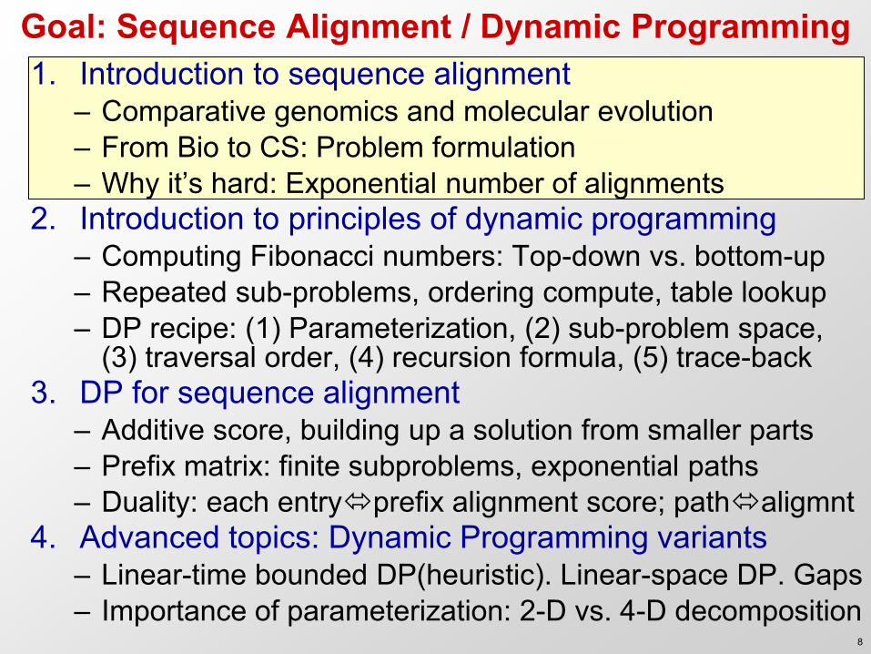
Goal: Sequence Alignment / Dynamic Programming 1. Introduction to sequence alignment

– Comparative genomics and molecular evolution – From Bio to CS: Problem formulation – Why it’s hard: Exponential number of alignments

2. Introduction to principles of dynamic programming – Computing Fibonacci numbers: Top-down vs. bottom-up – Repeated sub-problems, ordering compute, table lookup – DP recipe: (1) Parameterization, (2) sub-problem space,

(3) traversal order, (4) recursion formula, (5) trace-back 3. DP for sequence alignment

– Additive score, building up a solution from smaller parts – Prefix matrix: finite subproblems, exponential paths – Duality: each entryprefix alignment score; pathaligmnt

4. Advanced topics: Dynamic Programming variants – Linear-time bounded DP(heuristic). Linear-space DP. Gaps – Importance of parameterization: 2-D vs. 4-D decomposition

8

Genomes change over time

A C G T C A T C A

A C G T G A T C A mutation

A G T G T C A

A G T G T C A

deletion

A G T G T C A T

begin

end

A G T G T C A T insertion

9

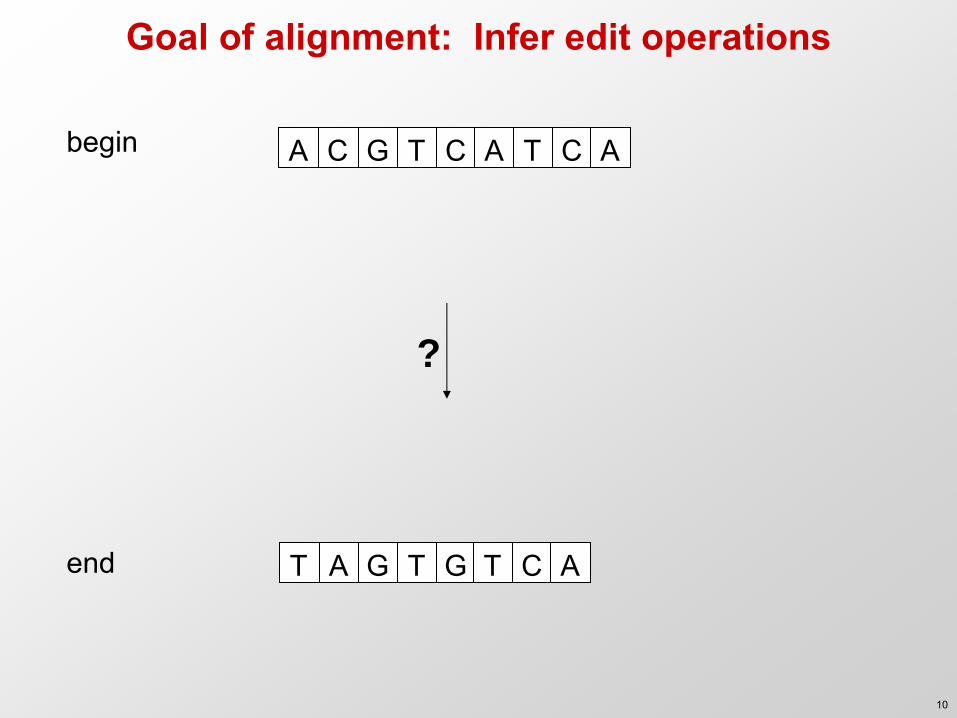
Goal of alignment: Infer edit operations

A C G T C A T C A

A G T G T C A T

begin

end

?

10

From Bio to CS: Formalizing the problem • Define set of evolutionary operations (insertion, deletion, mutation)

– Symmetric operations allow time reversibility (part of design choice)

(Exception: methylated CpG dinucleotides TpG/CpA non-symmetric)

Human Mouse

Many possible transformations

Minimum cost transformation(s)

• Define optimality criterion (min number, min cost) –Impossible to infer exact series of operations (Occam’s razor: find min)

• Design algorithm that achieves that optimality (or approximates it) –Tractability of solution depends on assumptions in the formulation

Human Mouse Human Mouse

Human Mouse x y x y x+y

Bio CS Relevance Assumptions

Special cases Tractability Tradeoffs

Computability

Algorithms

Implementation

Predictability

Correctness

Note: Not all decisions are conflicting (some are both relevant and tractable) (e.g. Pevzner vs. Sankoff and directionality in chromosomal inversions) 11

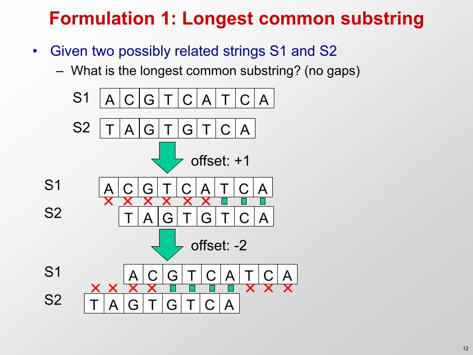
Formulation 1: Longest common substring • Given two possibly related strings S1 and S2

– What is the longest common substring? (no gaps) A C G T C A T C A

T A G T G T C A

S1

S2

A C G T C A T C A S1

S2 T A G T G T C A

offset: +1

A C G T C A T C A S1

S2 T A G T G T C A

offset: -2

12

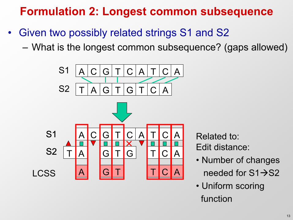
Formulation 2: Longest common subsequence

• Given two possibly related strings S1 and S2 – What is the longest common subsequence? (gaps allowed)

A C G T C A T C A

T A G T G T C A

S1

S2

A C G T C A T C A

T A G T G T C A

S1

S2

A C G T C A T C A

T A G T G T C A

S1

S2

A G T T C A LCSS

Related to: Edit distance: • Number of changes needed for S1S2 • Uniform scoring function

13

Formulation 3: Sequence alignment

• Allow gaps (fixed penalty) – Insertion & deletion operations – Unit cost for each character inserted or deleted

• Varying penalties for edit operations – Transitions (PyrimidinePyrimidine, PurinePurine) – Transversions (Purine Pyrimidine changes) – Polymerase confuses Aw/G and Cw/T more often

A G T C A +1 -½ -1 -1 G -½ +1 -1 -1 T -1 -1 +1 -½ C -1 -1 -½ +1

Scoring function: Match(x,x) = +1 Mismatch(A,G)= -½ Mismatch(C,T)= -½ Mismatch(x,y) = -1

Transitions: AG, CT common

(lower penalty) Transversions: All other operations

purine pyrimid. 14

Formulation 4: Varying gap cost models

1. Linear gap penalty – Same as before

2. Affine gap penalty – Big initial cost for starting or ending a gap – Small incremental cost for each additional character

3. General gap penalty – Any cost function – No longer computable using the same model

4. Frame-aware gap penalty – Multiples of 3 disrupt coding regions

5. Seek duplicated regions, rearrangements, … – Etc

15

How many alignments are there?

• Longest ‘non-boring’ alignment: n+m entries – Otherwise a gap will be aligned to a gapcondense

• Alignment is equivalent to gap placement – (n+m choose n) ways to choose S1 placement – At each position yes/no answer of placing character – Exponential number of possible placements

• Exponential number of sequence alignment – Enumerating and scoring each of them not an option – Need faster solution for finding best alignment

A C G T C A T C A

G T C A

S1

S2 G T A T

Need polynomial algorithm to find best alignment amongst an exponential number of possible alignments! DP

16







17

A simple introduction to the principles of Dynamic Programming

Turning exponentials into polynomials

18

Computing Fibonacci Numbers

• Fibonacci numbers

5

8

13

21

34

55

3 2

F6=F5+F4=(F4+F3)+(F3+F2))=….=(3+2)+(2+1)=5+3=8

© source unknown. All rights reserved. This content is excluded from our Creative

Commons license. For more information, see http://ocw.mit.edu/help/faq-fair-use/.

19


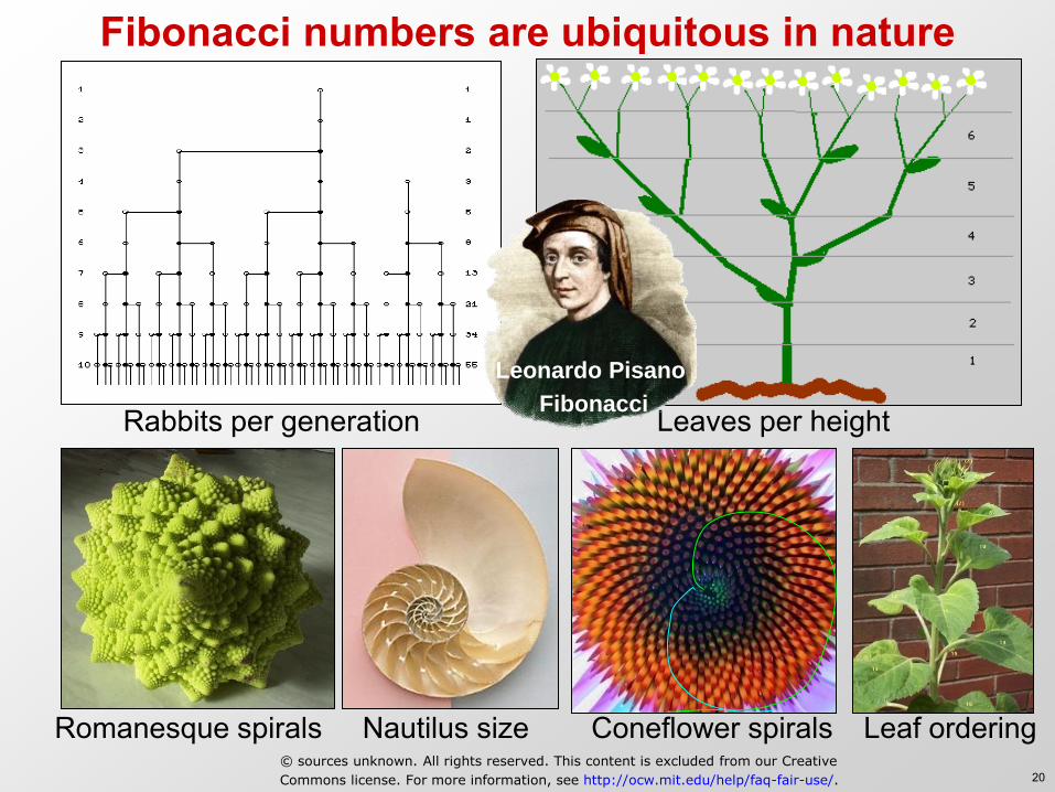
Fibonacci numbers are ubiquitous in nature

Rabbits per generation Leaves per height

Romanesque spirals Nautilus size Coneflower spirals Leaf ordering

Leonardo Pisano

Fibonacci

© sources unknown. All rights reserved. This content is excluded from our Creative

Commons license. For more information, see http://ocw.mit.edu/help/faq-fair-use/. 20


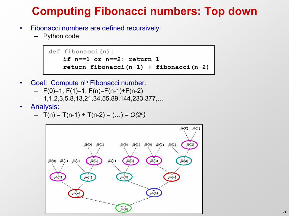
Computing Fibonacci numbers: Top down • Fibonacci numbers are defined recursively:

– Python code def fibonacci(n):

if n==1 or n==2: return 1

return fibonacci(n-1) + fibonacci(n-2)

• Goal: Compute nth Fibonacci number. – F(0)=1, F(1)=1, F(n)=F(n-1)+F(n-2) – 1,1,2,3,5,8,13,21,34,55,89,144,233,377,…

• Analysis: – T(n) = T(n-1) + T(n-2) = (…) = O(2n)

21

Computing Fibonacci numbers: Bottom up • Bottom up approach

– Python code

– Analysis: T(n) = O(n)

def fibonacci(n):

fib_table[1] = 1

fib_table[2] = 1

for i in range(3,n+1):

fib_table[i] = fib_table[i-1]+fib_table[i-2]

return fib_table[n]

? F[12] 89 F[11] 55 F[10] 34 F[9] 21 F[8] 13 F[7] 8 F[6] 5 F[5] 3 F[4] 2 F[3] 1 F[2] 1 F[1]

fib_table

22

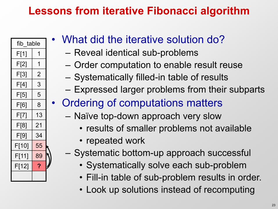
Lessons from iterative Fibonacci algorithm

• What did the iterative solution do? – Reveal identical sub-problems – Order computation to enable result reuse – Systematically filled-in table of results – Expressed larger problems from their subparts

• Ordering of computations matters – Naïve top-down approach very slow

• results of smaller problems not available • repeated work

– Systematic bottom-up approach successful • Systematically solve each sub-problem • Fill-in table of sub-problem results in order. • Look up solutions instead of recomputing

? F[12] 89 F[11] 55 F[10] 34 F[9] 21 F[8] 13 F[7] 8 F[6] 5 F[5] 3 F[4] 2 F[3] 1 F[2] 1 F[1]

fib_table

23

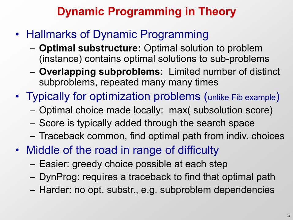
Dynamic Programming in Theory

• Hallmarks of Dynamic Programming – Optimal substructure: Optimal solution to problem

(instance) contains optimal solutions to sub-problems – Overlapping subproblems: Limited number of distinct

subproblems, repeated many many times • Typically for optimization problems (unlike Fib example)

– Optimal choice made locally: max( subsolution score) – Score is typically added through the search space – Traceback common, find optimal path from indiv. choices

• Middle of the road in range of difficulty – Easier: greedy choice possible at each step – DynProg: requires a traceback to find that optimal path – Harder: no opt. substr., e.g. subproblem dependencies

24

Hallmarks of optimization problems

1. Optimal substructure An optimal solution to a problem (instance) contains optimal solutions to subproblems.

2. Overlapping subproblems A recursive solution contains a “small” number

of distinct subproblems repeated many times.

3. Greedy choice property Locally optimal choices lead to globally optimal solution

Greedy algorithms Dynamic Programming

Greedy Choice is not possible

Globally optimal solution requires trace back through many choices

25

Dynamic Programming in Practice

• Setting up dynamic programming 1. Find ‘matrix’ parameterization (# dimensions, variables) 2. Make sure sub-problem space is finite! (not exponential)

• If not all subproblems are used, better off using memoization • If reuse not extensive, perhaps DynProg is not right solution!

3. Traversal order: sub-results ready when you need them • Computation order matters! (bottom-up, but not always

obvious) 4. Recursion formula: larger problems = F(subparts) 5. Remember choices: typically F() includes min() or max()

• Need representation for storing pointers, is this polynomial ! • Then start computing

1. Systematically fill in table of results, find optimal score 2. Trace-back from optimal score, find optimal solution

26







27

(3) How do we apply dynamic programming

to sequence alignment ?

28

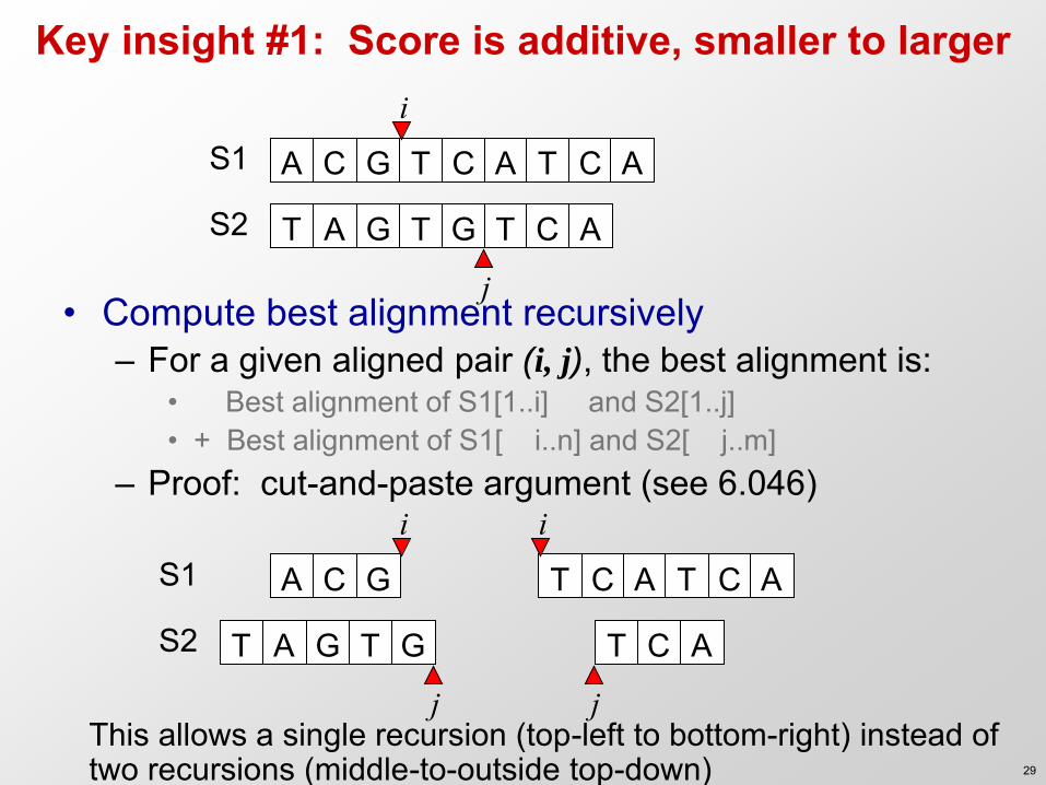
Key insight #1: Score is additive, smaller to larger

• Compute best alignment recursively – For a given aligned pair (i, j), the best alignment is:

• Best alignment of S1[1..i] and S2[1..j] • + Best alignment of S1[ i..n] and S2[ j..m]

– Proof: cut-and-paste argument (see 6.046)

A C G T C A T C A

T A G T G T C A

S1

S2

i

j

A C G T C A T C A

T A G T G T C A

S1

S2

i

j

i

j This allows a single recursion (top-left to bottom-right) instead of two recursions (middle-to-outside top-down) 29

Key insight #2: compute scores recursively

A C G T C A T C A

T A G T G T C A

S1

S2

A C G T

T A G T G

S1

S2

A C G T C A T C A

T A G T G T C A

S1

S2

Compute alignment of CGT vs. TG exactly once 30

Key insight #3: sub-problems are repeated reuse!

A C G T C A T C A

T A G T G T C A

S1

S2

A C G T

T A G T G

S1

S2

A C G T C A T C A

T A G T G T C A

S1

S2

S2

A C G T C A T C A

T A G T G T C A

S1

S2

A C G T C A T C A

T A G T G T C A

S1

C G T C A T C A

T G T C A

S1

S2

Identical sub-problems! We can reuse our work! 31

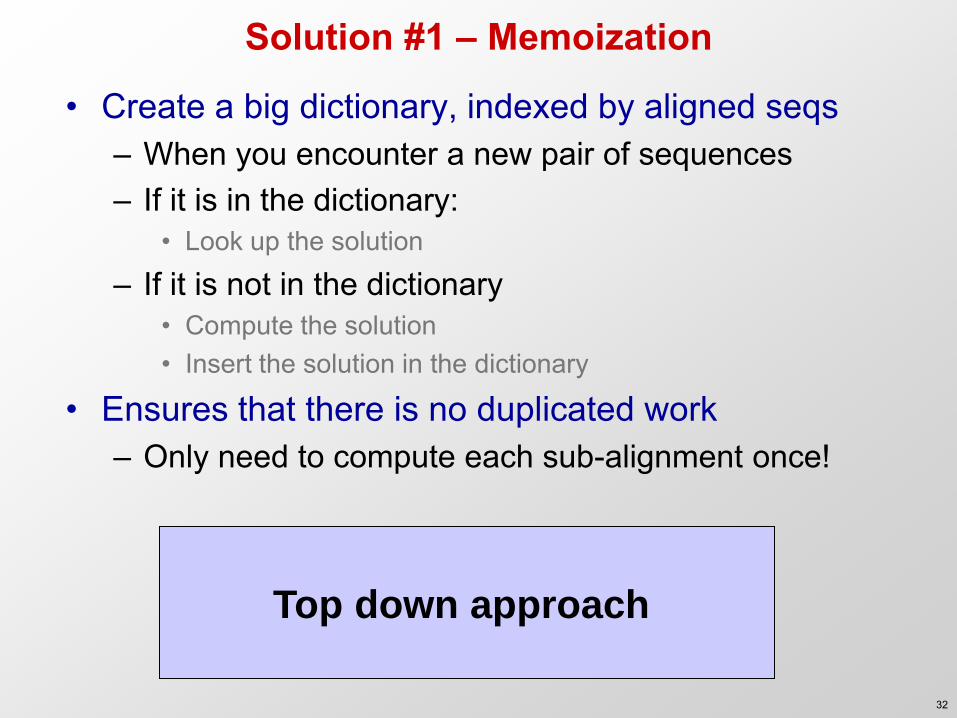
Solution #1 – Memoization

• Create a big dictionary, indexed by aligned seqs – When you encounter a new pair of sequences – If it is in the dictionary:

• Look up the solution

– If it is not in the dictionary • Compute the solution • Insert the solution in the dictionary

• Ensures that there is no duplicated work – Only need to compute each sub-alignment once!

Top down approach

32

Solution #2 – Dynamic programming

• Create a big table, indexed by (i,j) – Fill it in from the beginning all the way till the end – You know that you’ll need every subpart – Guaranteed to explore entire search space

• Ensures that there is no duplicated work – Only need to compute each sub-alignment once!

• Very simple computationally!

Bottom up approach

33

Key insight #4: Optimal prefix almt score Matrix entry

S1[1..i] i S1[i..n]

S2[1..j]

j S

S2[ j..m]

34

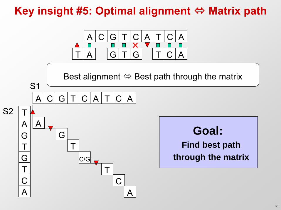
Key insight #5: Optimal alignment Matrix path

A C G T C A T C A T A G T G T C A

S1

S2

A C G T C A T C A

T A G T G T C A

A G

T C/G

T C

A

Goal: Find best path

through the matrix

Best alignment Best path through the matrix

35

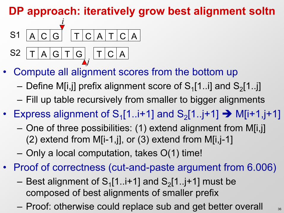
DP approach: iteratively grow best alignment soltn

• Compute all alignment scores from the bottom up – Define M[i,j] prefix alignment score of S1[1..i] and S2[1..j] – Fill up table recursively from smaller to bigger alignments

• Express alignment of S1[1..i+1] and S2[1..j+1] M[i+1,j+1] – One of three possibilities: (1) extend alignment from M[i,j]

(2) extend from M[i-1,j], or (3) extend from M[i,j-1] – Only a local computation, takes O(1) time!

• Proof of correctness (cut-and-paste argument from 6.006) – Best alignment of S1[1..i+1] and S2[1..j+1] must be

composed of best alignments of smaller prefix – Proof: otherwise could replace sub and get better overall

A C G T C A T C A

T A G T G T C A

S1

S2

i

j

36

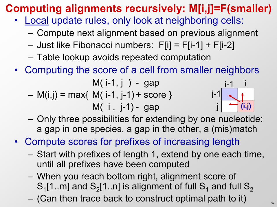
Computing alignments recursively: M[i,j]=F(smaller) • Local update rules, only look at neighboring cells:

– Compute next alignment based on previous alignment – Just like Fibonacci numbers: F[i] = F[i-1] + F[i-2] – Table lookup avoids repeated computation

• Computing the score of a cell from smaller neighbors M( i-1, j ) - gap – M(i,j) = max{ M( i-1, j-1) + score } M( i , j-1) - gap – Only three possibilities for extending by one nucleotide:

a gap in one species, a gap in the other, a (mis)match • Compute scores for prefixes of increasing length

– Start with prefixes of length 1, extend by one each time, until all prefixes have been computed

– When you reach bottom right, alignment score of S1[1..m] and S2[1..n] is alignment of full S1 and full S2

– (Can then trace back to construct optimal path to it)

(i,j)

i-1 i j-1

j

37

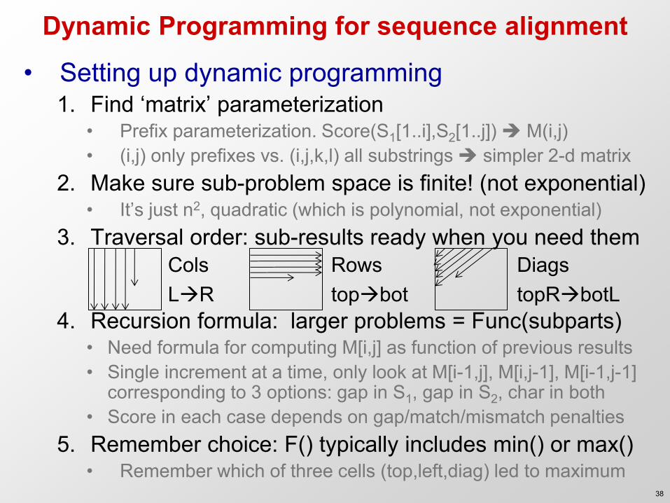
Dynamic Programming for sequence alignment

• Setting up dynamic programming 1. Find ‘matrix’ parameterization

• Prefix parameterization. Score(S1[1..i],S2[1..j]) M(i,j) • (i,j) only prefixes vs. (i,j,k,l) all substrings simpler 2-d matrix

2. Make sure sub-problem space is finite! (not exponential) • It’s just n2, quadratic (which is polynomial, not exponential)

3. Traversal order: sub-results ready when you need them

4. Recursion formula: larger problems = Func(subparts) • Need formula for computing M[i,j] as function of previous results • Single increment at a time, only look at M[i-1,j], M[i,j-1], M[i-1,j-1]

corresponding to 3 options: gap in S1, gap in S2, char in both • Score in each case depends on gap/match/mismatch penalties

5. Remember choice: F() typically includes min() or max() • Remember which of three cells (top,left,diag) led to maximum

Cols LR

Rows topbot

Diags topRbotL

38

Step 1: Setting up the scoring matrix M[i,j] - A G T

A

A

G

C

- 0 Initialization: • Top left: 0 Update Rule: M(i,j)=max{

} Termination: • Bottom right

39

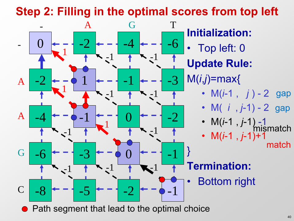
Step 2: Filling in the optimal scores from top left - A G T

A

A

G

C

- 0 -2

-2 1

-1 0

0 -1

-4 -6

-1 -3

-4 -2

-6 -3

-8 -5 -2 -1

-1 -1

-1 -1

-1 -1

-1 -1

-1

Initialization: • Top left: 0 Update Rule: M(i,j)=max{

• M(i-1 , j ) - 2 • M( i , j-1) - 2 • M(i-1 , j-1) -1 • M(i-1 , j-1)+1


mismatch

match

gap gap

1

1

1

Path segment that lead to the optimal choice 40

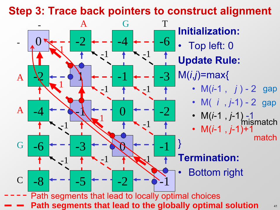
Step 3: Trace back pointers to construct alignment - A G T

A

A

G

C

- 0 -2 -4 -6

-2 1 -1 -3

-4 -1 0 -2

-6 -3 0 -1

-8 -5 -2 -1

-1 -1

-1 -1

-1 -1

-1 -1

-1

Initialization: • Top left: 0 Update Rule: M(i,j)=max{

• M(i-1 , j ) - 2 • M( i , j-1) - 2 • M(i-1 , j-1) -1 • M(i-1 , j-1)+1


1

1

1 mismatch

match

gap gap

Path segments that lead to the globally optimal solution Path segments that lead to locally optimal choices

41

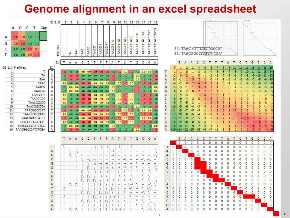
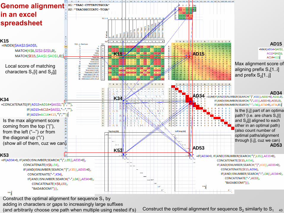
Genome alignment in an excel spreadsheet

42

K15

K34

K53 AD53

AD34

AD15

K15

K34

K53

AD53

AD34

AD15

Local score of matching characters S1[i] and S2[j]

Max alignment score of aligning prefix S1[1..i] and prefix S2[1..j]

Is the max alignment score coming from the top (“|”), from the left (“--”) or from the diagonal up (“\”) (show all of them, cuz we can)

Is the [i,j] part of an optimal path? (i.e. are chars S1[i] and S2[j] aligned to each other in an optimal path) (also count number of optimal paths/alignment through [i.j], cuz we can)

Construct the optimal alignment for sequence S1 by adding in characters or gaps to increasingly large suffixes (and arbitrarily choose one path when multiple using nested if’s) Construct the optimal alignment for sequence S2 similarly to S1

Genome alignment in an excel spreadsheet

43

What is missing? (5) Returning the actual path!

• We know how to compute the best score – Simply the number at the bottom right entry

• But we need to remember where it came from – Pointer to the choice we made at each step

• Retrace path through the matrix – Need to remember all the pointers

Time needed: O(m*n) Space needed: O(m*n)

x1 ………………………… xM

y1 …

……

……

……

……

…

yN

44







45

If time permits…

(4) Extensions to basic DP solution

46

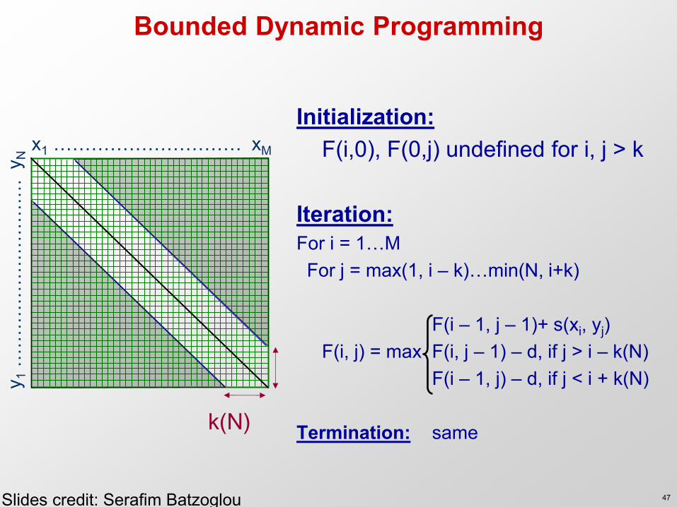
Bounded Dynamic Programming

Initialization: F(i,0), F(0,j) undefined for i, j > k Iteration: For i = 1…M For j = max(1, i – k)…min(N, i+k) F(i – 1, j – 1)+ s(xi, yj) F(i, j) = max F(i, j – 1) – d, if j > i – k(N) F(i – 1, j) – d, if j < i + k(N) Termination: same

x1 ………………………… xM

y1 …

……

……

……

……

… y

N

k(N)

Slides credit: Serafim Batzoglou 47

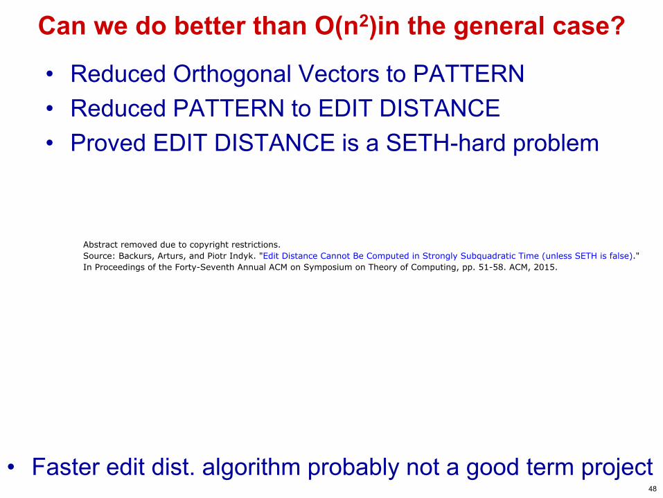
Can we do better than O(n2)in the general case?

• Reduced Orthogonal Vectors to PATTERN • Reduced PATTERN to EDIT DISTANCE • Proved EDIT DISTANCE is a SETH-hard problem

• Faster edit dist. algorithm probably not a good term project 48

Abstract removed due to copyright restrictions. Source: Backurs, Arturs, and Piotr Indyk. "Edit Distance Cannot Be Computed in Strongly Subquadratic Time (unless SETH is false)."In Proceedings of the Forty-Seventh Annual ACM on Symposium on Theory of Computing, pp. 51-58. ACM, 2015.

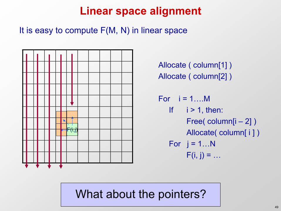
http://dx.doi.org/10.1145/2746539.2746612

F(i,j)

Linear space alignment It is easy to compute F(M, N) in linear space

Allocate ( column[1] ) Allocate ( column[2] ) For i = 1….M If i > 1, then: Free( column[i – 2] ) Allocate( column[ i ] ) For j = 1…N F(i, j) = …

What about the pointers? 49

Finding the best back-pointer for current column

• Now, using 2 columns of space, we can compute for k = 1…M, F(M/2, k), Fr(M/2, N-k) PLUS the backpointers

50

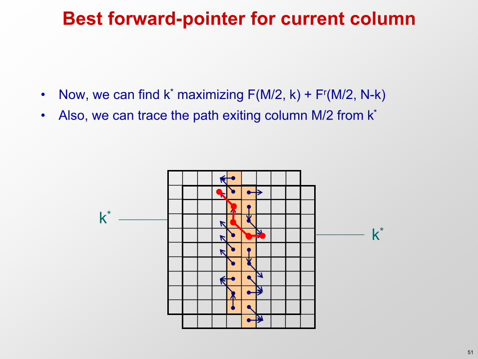
Best forward-pointer for current column

• Now, we can find k* maximizing F(M/2, k) + Fr(M/2, N-k) • Also, we can trace the path exiting column M/2 from k*

k* k*

51

Recursively find midpoint for left & right

• Iterate this procedure to the left and right!

N-k*

M/2 M/2

k*

52

Total time cost of linear-space alignment

Total Time: cMN + cMN/2 + cMN/4 + ….. = 2cMN = O(MN) Total Space: O(N) for computation, O(N+M) to store the optimal alignment

N-k*

M/2 M/2

k*

53







54

Additional insights

Why the 2-dimentional parameterization worked

55

Summary • Dynamic programming

– Reuse of computation – Order sub-problems. Fill table of sub-problem results – Read table instead of repeating work (ex: Fibonacci)

• Sequence alignment – Edit distance and scoring functions – Dynamic programming matrix – Matrix traversal path Optimal alignment

• Thursday: Variations on sequence alignment – Local/global alignment, affine gaps, algo speed-ups – Semi-numerical alignment, hashing, database lookup

• Recitation: – Dynamic programming applications – Probabilistic derivations of alignment scores

56







57

MIT OpenCourseWarehttp://ocw.mit.edu

6.047 / 6.878 / HST.507 Computational BiologyFall 2015

For information about citing these materials or our Terms of Use, visit: http://ocw.mit.edu/terms.

http://ocw.mit.edu

http://ocw.mit.edu/terms

lecture 2 sequence alignment and dynamic programming · sequence alignment and dynamic programming...

Documents