sequence alignment and dynamic programming
TRANSCRIPT

6.096 – Algorithms for Computational Biology
Sequence Alignment
and Dynamic Programming
Lecture 1 - Introduction
Lecture 2 - Hashing and BLAST
Lecture 3 - Combinatorial Motif Finding
Lecture 4 - Statistical Motif Finding
5
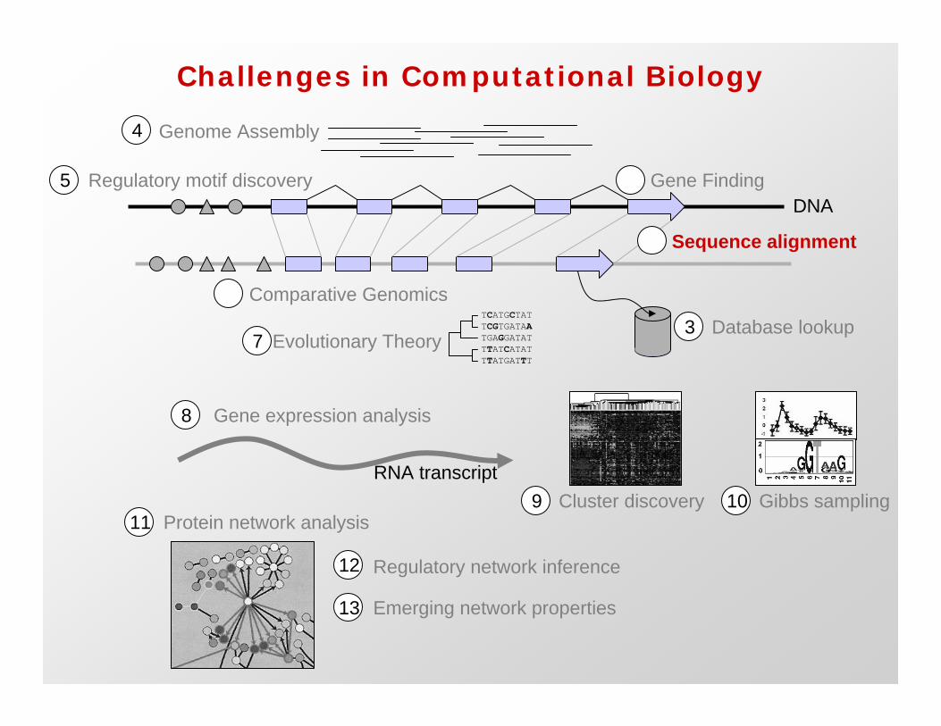
Challenges in Computational Biology
4 Genome Assembly
Regulatory motif discovery 1 Gene Finding
DNA
2 Sequence alignment
6 Comparative Genomics TCATGCTAT TCGTGATAA 3 Database lookup
7 Evolutionary Theory TGAGGATAT TTATCATAT TTATGATTT
8 Gene expression analysis
RNA transcript
Protein network analysis11 9 Gibbs sampling10
12 Regulatory network inference
Emerging network properties13
Cluster discovery
A C G T C A T C A
T A G T G T C A
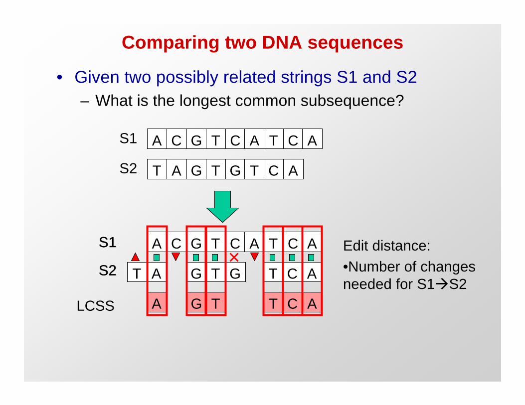
Comparing two DNA sequences
• Given two possibly related strings S1 and S2
– What is the longest common subsequence?
A C G T C A T C A
T A G T G T C A
S1
S2
S1S1 A C G T C A T C A
T A G T G T C A
A G T T C A
S2S2
LCSS
Edit distance:
•Number of changes
needed for S1ÆS2
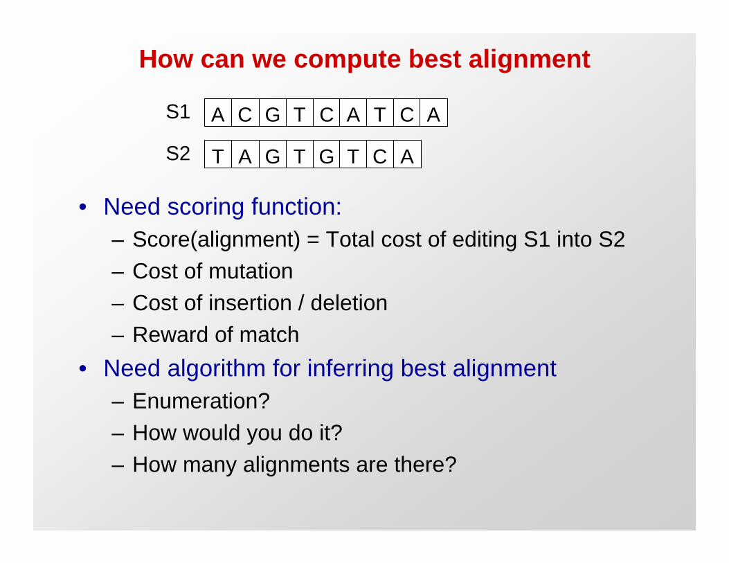
How can we compute best alignment
S1
S2
A C G T C A T C A
T A G T G T C A
• Need scoring function:
– Score(alignment) = Total cost of editing S1 into S2
– Cost of mutation
– Cost of insertion / deletion
– Reward of match
• Need algorithm for inferring best alignment
– Enumeration?
– How would you do it?
– How many alignments are there?
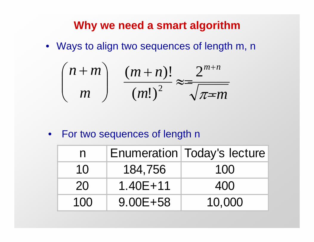
Why we need a smart algorithm
• Ways to align two sequences of length m, n
n m�§¨
m�n· (m�n)! |
2
�S ¸¹¸ (m!)2
© m m
• For two sequences of length n
n Enumeration Today's lecture
10 184,756 100
20 1.40E+11 400
100 9.00E+58 10,000
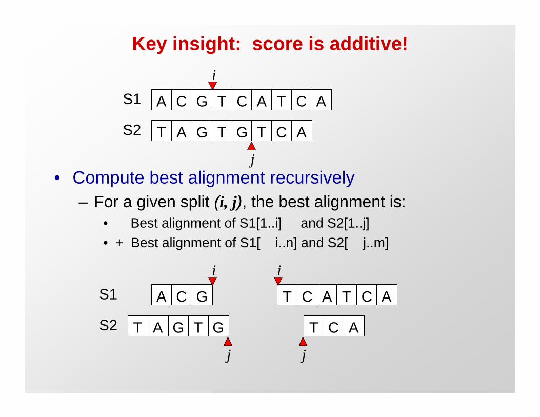
Key insight: score is additive!
A C G T C A T C A
T A G T G T C A
S1
S2
i
j
• Compute best alignment recursively
– For a given split (i, j), the best alignment is:
• Best alignment of S1[1..i] and S2[1..j]
• + Best alignment of S1[ i..n] and S2[ j..m]
i i
A C G T C A T C A
T A G T G T C A
S1
S2
j j
A C G T C A T C A
T A G T G T C A
S1
S2
A C G T
T A G T G
S1
S2
A C G T C A T C A
T A G T G T C A
S1
S2
S2
A C G T C A T C A
T A G T G T C A
S1
S2
A C G T C A T C A
T A G T G T C A
S1
C G T C A T C A
T G T C A
S1
S2
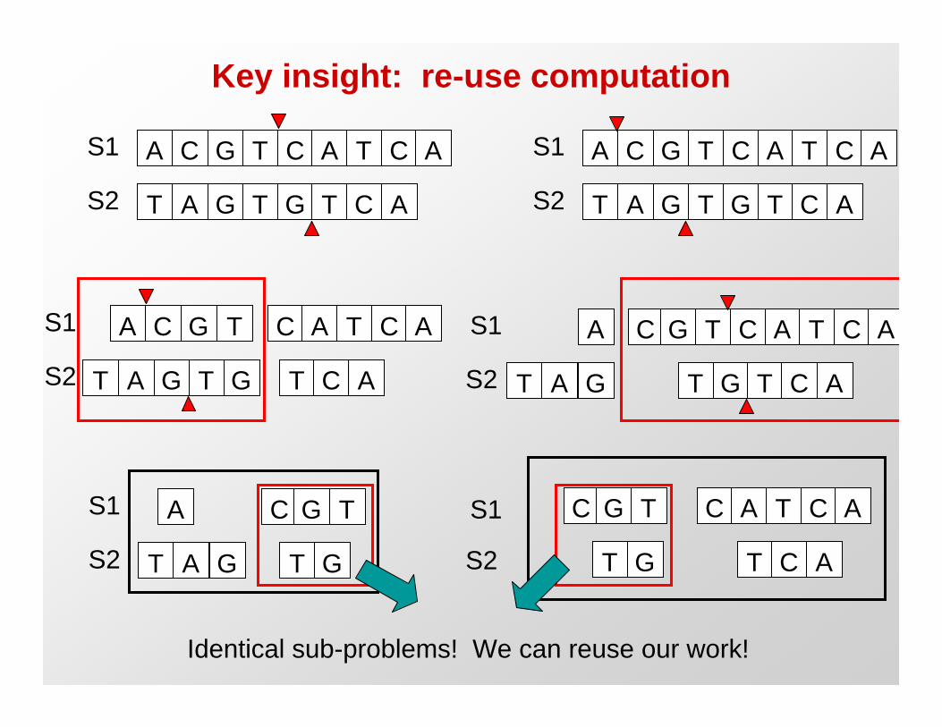
Key insight: re-use computation
Identical sub-problems! We can reuse our work!
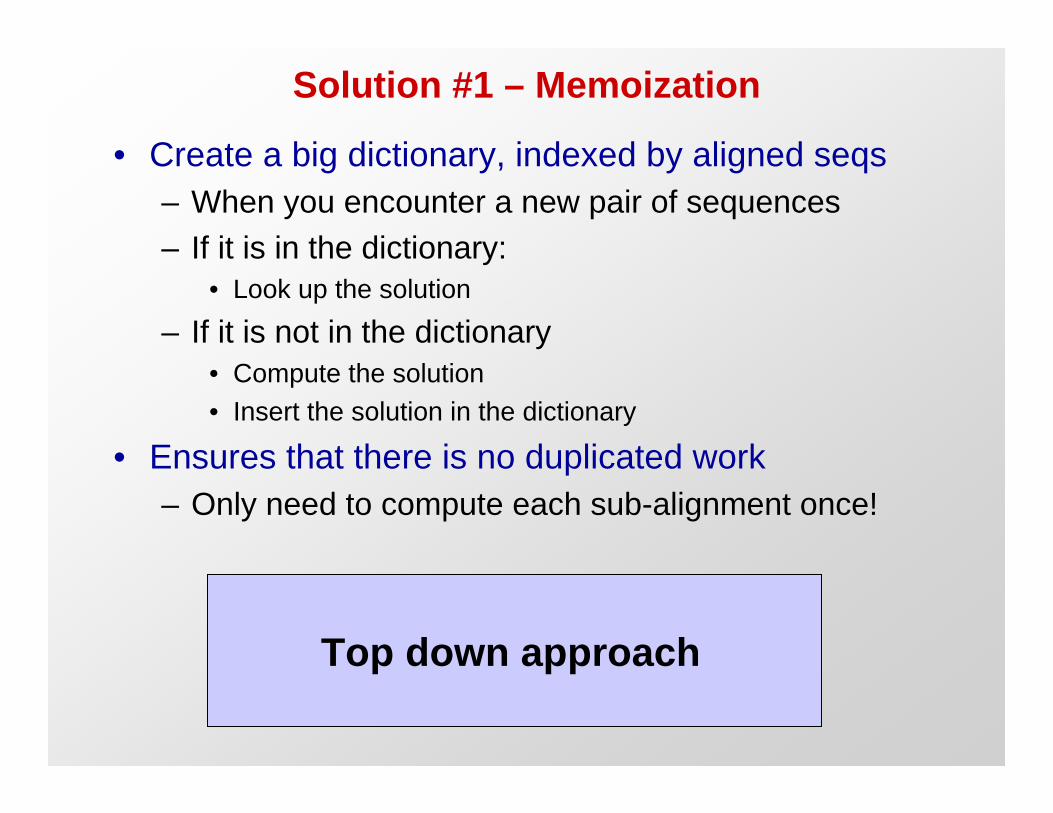
Solution #1 – Memoization
• Create a big dictionary, indexed by aligned seqs
– When you encounter a new pair of sequences
– If it is in the dictionary:
• Look up the solution
– If it is not in the dictionary
• Compute the solution
• Insert the solution in the dictionary
• Ensures that there is no duplicated work
– Only need to compute each sub-alignment once!
Top down approach

Solution #2 – Dynamic programming
• Create a big table, indexed by (i,j)
– Fill it in from the beginning all the way till the end
– You know that you’ll need every subpart
– Guaranteed to explore entire search space
• Ensures that there is no duplicated work
– Only need to compute each sub-alignment once!
• Very simple computationally!
Bottom up approach

A C G T C A T C A
T A G T G T C A
S1
S2
A C G T C A T C A
T
A
G
T
G
T
C
A
A
G
T
C/G
T
C
A
Goal: Find best path
through the matrix
Key insight: Matrix representation of alignments
Sequence alignment
Dynamic Programming
Global alignment
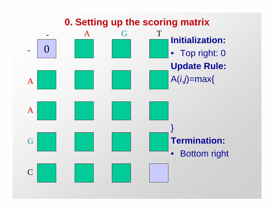
0. Setting up the scoring matrix
- A G T
A
A
G
C
- 0 Initialization:
•
Update Rule:
A(i,j)=max{
}
Termination:
•
Top right: 0
Bottom right

1. Allowing gaps in s
- A G T
A
A
G
C
- 0
-2
-4
-6
-8
Initialization:
•
Update Rule:
A(i,j)=max{
i-1 , j
}
Termination:
•
Top right: 0
Bottom right
• A( ) - 2
0
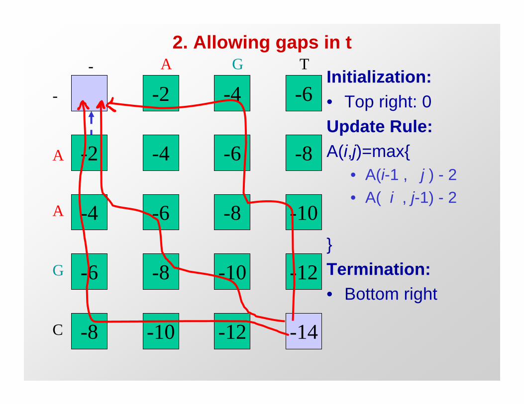
2. Allowing gaps in t
- A G T
-
A
A
G
-2 -4 -6
-2 -4 -6 -8
-4 -6 -8 -10
-6 -8 -10 -12
-8 -10 -12 -14
Initialization:
• Top right: 0
Update Rule:
A(i,j)=max{
• A(i-1 , j ) - 2
• A( i , j-1) - 2
}
Termination:
• Bottom right
C

3. Allowing mismatches
- A G T
-
A
A
G
0 -2 -4 -6
-2 -1 -3 -5
-4 -3 -2 -4
-6 -5 -4 -3
-8 -7 -6 -5
-1
-1
-1
-1 -1
-1 -1
-1 -1
-1 -1
-1
Initialization:
• Top right: 0
Update Rule:
A(i,j)=max{
• A(i-1 , j ) - 2
• A( i , j-1) - 2
• A(i-1 , j-1) -1
}
Termination:
• Bottom right
C
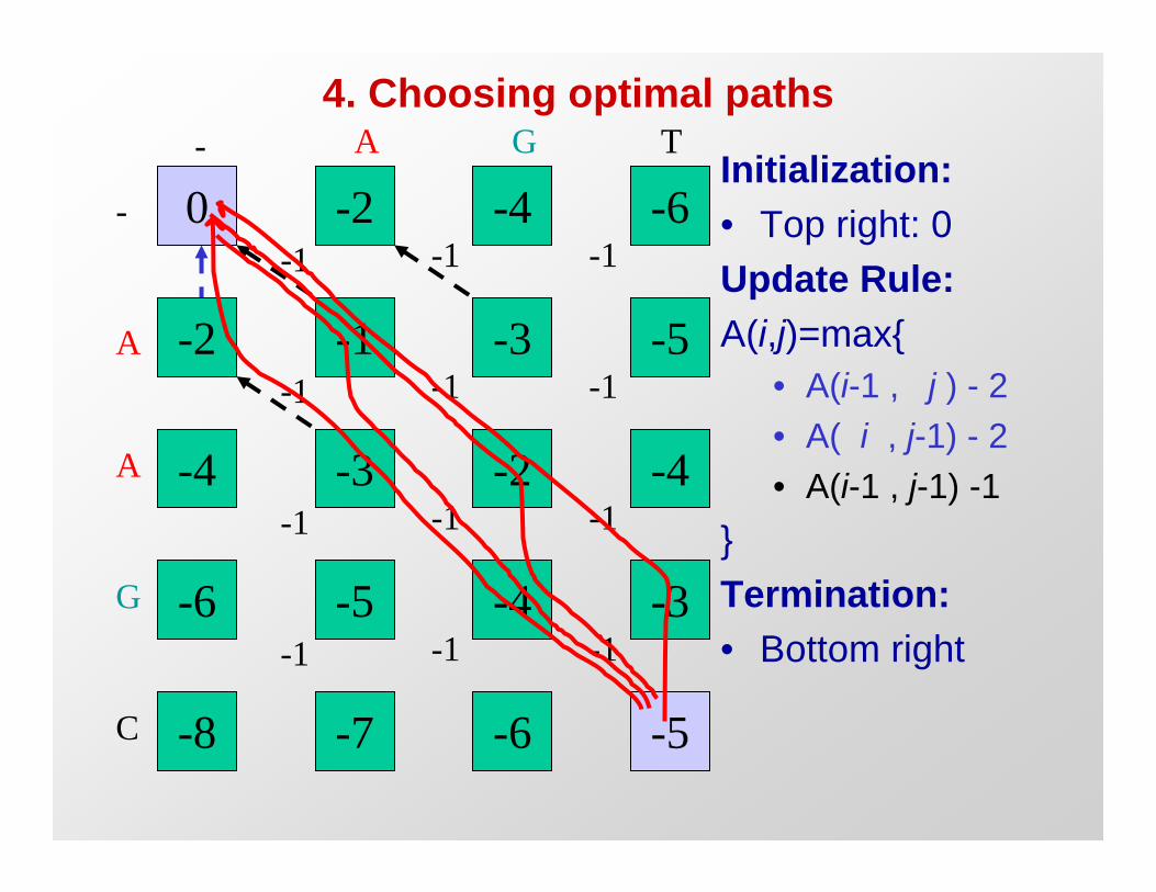
4. Choosing optimal paths
- A G T
-
A
A
G
0 -2 -4 -6
-2 -1 -3 -5
-4 -3 -2 -4
-6 -5 -4 -3
-8 -7 -6 -5
-1
-1
-1
-1 -1
-1 -1
-1 -1
-1 -1
-1
Initialization:
• Top right: 0
Update Rule:
A(i,j)=max{
• A(i-1 ,
• A( i ,
• A(i-1 ,
}
j ) - 2
j-1) - 2
j-1) -1
Termination:
• Bottom right
C
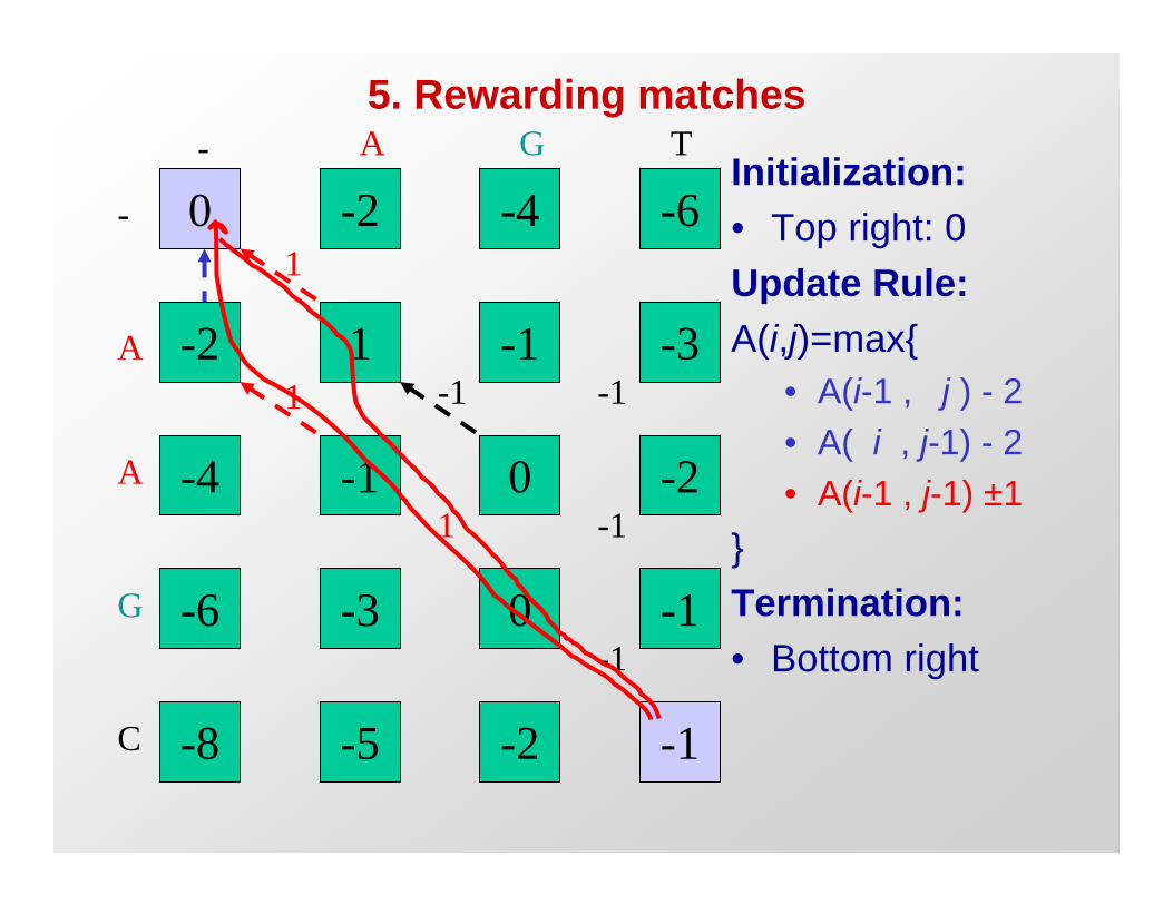
5. Rewarding matches
- A G T
-
A
A
G
0 -2 -4 -6
-2 1 -1 -3
-4 -1 0 -2
-6 -3 0 -1
-8 -5 -2 -1
1
1
1
-1 -1
-1
-1
Initialization:
• Top right: 0
Update Rule:
A(i,j)=max{
• A(i-1 ,
• A( i ,
• A(i-1 ,
}
j ) - 2
j-1) - 2
j-1) ±1
Termination:
• Bottom right
C
Sequence alignment
Global Alignment
Semi-Global
Dynamic Programming

Semi-Global Motivation
• Aligning the following sequencesCAGCACTTGGATTCTCGG
CAGC-----G-T----GG
• We might prefer the alignment
vvvv-----v-v----vv = 8(1)+0(-1)+10(-2) = -12
CAGCA-CTTGGATTCTCGG match mismatch ---CAGCGTGG--------
---vv-vxvvv-------- = 6(1)+1(-1)+12(-2) = -19
gap
• New qualities sought, new scoring scheme designed
– Intuitively, don’t penalize “missing” end of the sequence
–We’d like to model this intuition

Ignoring starting gaps
- A G T Initialization:
- / l• 1st row co : 0
Update Rule:
A(i,j)=max{A
• A(i-1 , j ) - 2
• A( i , j-1) - 2 A
• A(i-1 , j-1) ±1
}
Termination:G
• Bottom right
0 0 0 0
0 1 -1 -1
0 1 0 -2
0 -1 2 0
0 -1 0 1
1
1
1
-1
-1 -1
-1 -1
-1
-1
C
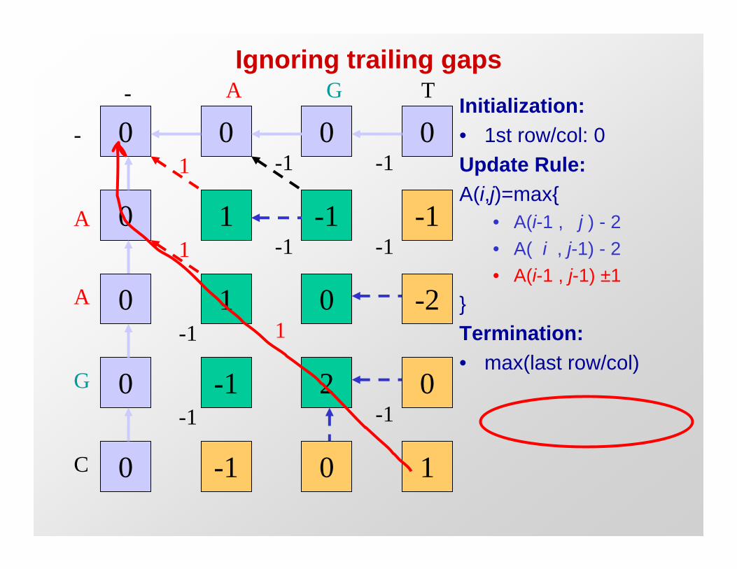
Ignoring trailing gaps
- A G T
-
A
A
G
0 0 0 0
0 1 -1 -1
0 1 0 -2
0 -1 2 0
0 -1 0 1
1
1
1
-1
-1 -1
-1 -1
-1
-1
Initialization:
• 1st row/col: 0
Update Rule:
A(i,j)=max{
• A(i-1 , j ) - 2
• A( i , j-1) - 2
• A(i-1 , j-1) ±1
}
Termination:
• max(last row/col)
C

Using the new scoring scheme
• With the old scoring scheme (all gaps count -2)
CAGCACTTGGATTCTCGG
CAGC-----G-T----GG
vvvv-----v-v----vv = 8(1)+0(-1)+10(-2)+0(-0) = -12
• New score (end gaps are free)
6(1)+1(-1)+1(-2)+11(-0) = 3
match mismatch gap CAGCA-CTTGGATTCTCGG
endgap---CAGCGTGG--------
---vv-vxvvv-------- =

Semi-global alignments
• Applications: query
– Finding a gene in a genome
– Aligning a read onto an assembly subject
– Finding the best alignment of a PCR primer
– Placing a marker onto a chromosome
• These situations have in common
– One sequence is much shorter than the other
– Alignment should span the entire length of the smaller
sequence
– No need to align the entire length of the longer sequence
• In our scoring scheme we should
– Penalize end-gaps for subject sequence
– Do not penalize end-gaps for query sequence

Semi-Global Alignment- A G T
-
A
A
G
C
Query: s
Subject: t
align all of s
Initialization:
•
Update Rule:
A(i,j)=max{
• A(i-1 , j
• A( i , j
• A(i-1 , j-1) ±1
}
Termination:
•
0 -2 -4 -6
0 1 -1 -1
0 1 0 -2
0 -1 2 1
0 -1 0 0
...or...
0 -2 -4 -6
-2 1 -1 -1
-4 1 0 -2
-6 -1 2 0
-8 -1 0 -1
- A G T
A
A
G
C
-Initialization:
•1st row
A(i,j)=max{
•A(i-1 , j
•A( i , j
•A(i-1 , j-1) ±1
}
Termination:
•max(last row)
Query: t
Subject: s
align all of t
1st col
max(last col)
) - 2
-1) - 2
Update Rule:
) - 2
-1) - 2

Sequence alignment
Global Alignment
Semi-Global
Local Alignment
Dynamic Programming

Intro to Local Alignments
• Statement of the problem
– A local alignment of strings s and t
is an alignment of a substring of s
with a substring of t
• Definitions (reminder):
– A substring consists of consecutive characters
– A subsequence of s needs not be contiguous in s
• Naïve algorithm
– Now that we know how to use dynamic programming
– Take all O((nm)2), and run each alignment in O(nm) time
• Dynamic programming
– By modifying our existing algorithms, we achieve O(mn)
s
t

Global Alignment
- A G T
-
A
A
G
0 -2 -4 -6
-2 1 -1 -5
-4 1 0 -2
-6 -1 2 0
-8 -1 0 1
1
1
1
-1
-1 -1
-1 -1
-1
-1
Initialization:
• Top left: 0
Update Rule:
A(i,j)=max{
• A(i-1 ,
• A( i ,
• A(i-1 ,
}
j ) - 2
j-1) - 2
j-1) ±1
Termination:
• Bottom right C

Local Alignment
- A G T
A
A
G
C
- 0 0 0 0
0 1 0 0
0 1 0 0
0 0 2 0
0 0 0 1
1
1
1
-1
Initialization:
•
Update Rule:
A(i,j)=max{
i-1 , j
i , j
i-1 , j-1) ±1
• 0
}
Termination:
• Anywhere
-1
Top left: 0
• A(
• A(
• A(
) - 2
-1) - 2

Local Alignment issues
• Resolving ambiguities
– When following arrows back, one can stop at any of the zero
entries. Only stop when no arrow leaves. Longest.
• Correctness sketch by induction
– Assume we’ve correctly aligned up to (i,j)
– Consider the four cases of our max computation
– By inductive hypothesis recurse on (i-1,j-1), (i-1,j), (i,j-1)
– Base case: empty strings are suffixes aligned optimally
• Time analysis
– O(mn) time
– O(mn) space, can be brought to O(m+n)

Sequence alignment
Global Alignment
Semi-Global
Local Alignment
Affine Gap Penalty
Dynamic Programming

Scoring the gaps more accurately
Current model:
J(n)Gap of length n
incurs penalty nud
However, gaps usually occur in bunches
Convex gap penalty function:
J(n):
for all n, J(n + 1) - J(n) d J(n) - J(n – 1) J(n)
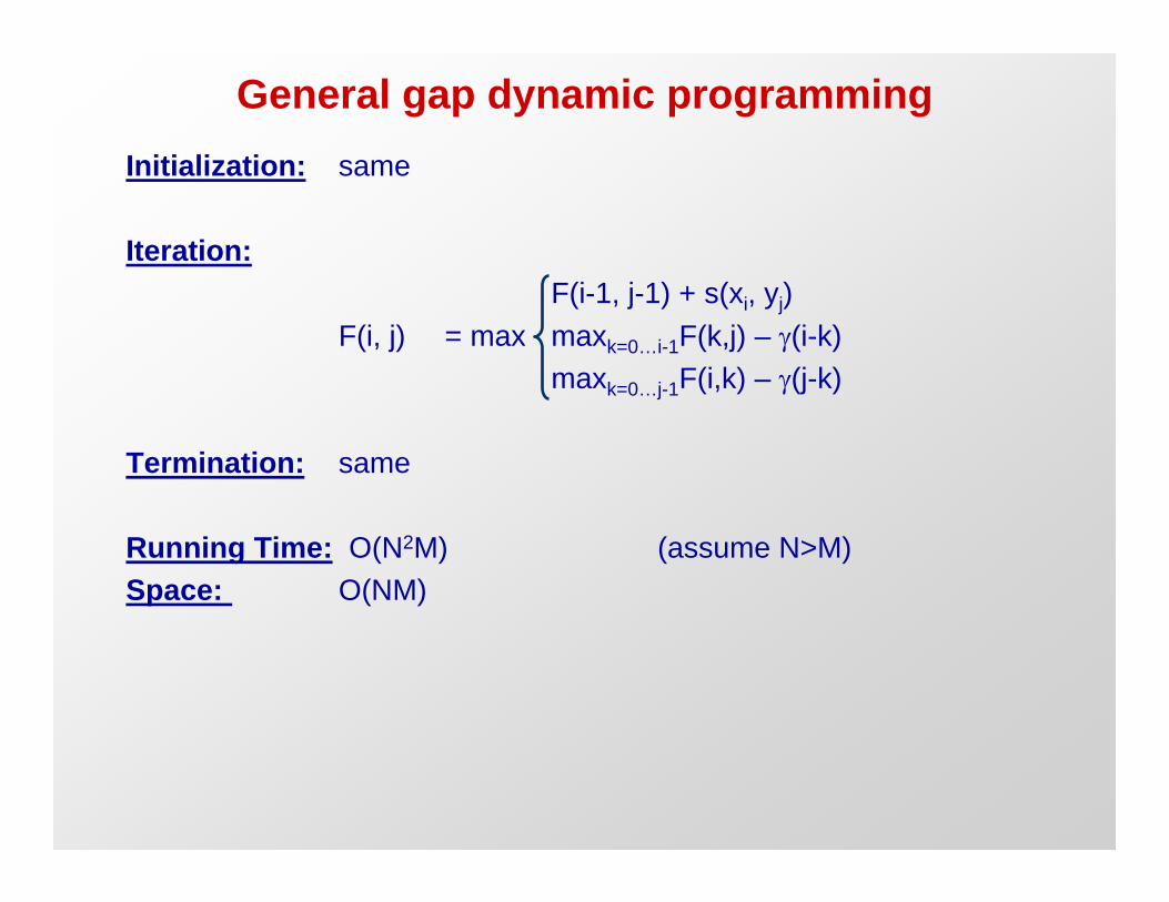
General gap dynamic programming
Initialization: same
Iteration:
F(i-1, j-1) + s(xi, yj)
F(i, j) = max
max
maxk=0…i-1F(k,j) – J(i-k)
k=0…j-1F(i,k) – J(j-k)
Termination: same
Running Time: O(N2M)
Space:
(assume N>M)
O(NM)

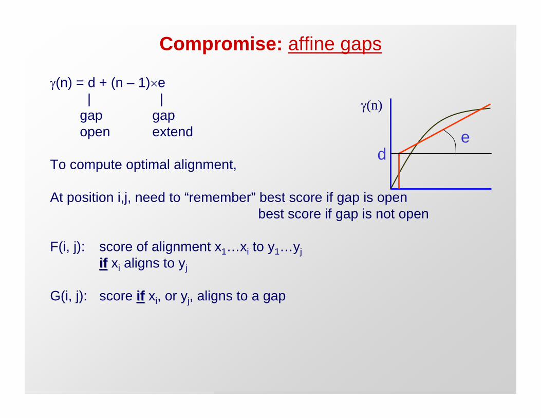
Compromise: affine gaps
J(n) = d + (n – 1)ue J(n)| |
gap gap
open extendd
To compute optimal alignment,
e
At position i,j, need to “remember” best score if gap is open
best score if gap is not open
F(i, j): score of alignment x1…xi to y1…yj
ifif xi aligns to yj
G(i, j): score ifif xi, or yj, aligns to a gap

Motivation for affine gap penalty
• Modeling evolution
– To introduce the first gap, a break must occur in DNA
– Multiple consecutive gaps likely to be introduced by the same
evolutionary event. Once the break is made, it’s relatively easy
to make multiple insertions or deletions.
– Fixed cost for opening a gap: p+q
– Linear cost increment for increasing number of gaps: q
• Affine gap cost function
– New gap function for length k: w(k) = p+q*k
– p+q is the cost of the first gap in a run
– q is the additional cost of each additional gap in same run
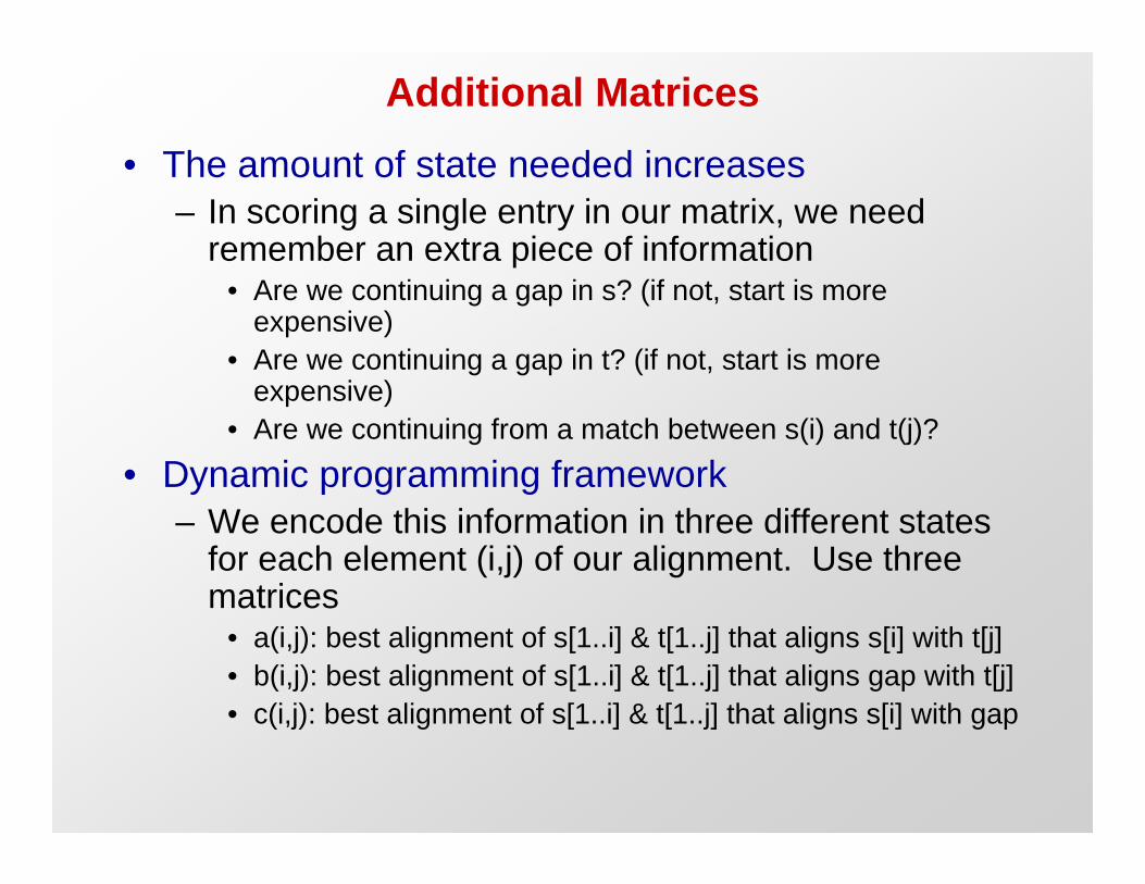
Additional Matrices
• The amount of state needed increases
– In scoring a single entry in our matrix, we need remember an extra piece of information
• Are we continuing a gap in s? (if not, start is more expensive)
• Are we continuing a gap in t? (if not, start is more expensive)
• Are we continuing from a match between s(i) and t(j)?
• Dynamic programming framework
– We encode this information in three different states for each element (i,j) of our alignment. Use three matrices
• a(i,j): best alignment of s[1..i] & t[1..j] that aligns s[i] with t[j]
• b(i,j): best alignment of s[1..i] & t[1..j] that aligns gap with t[j]
• c(i,j): best alignment of s[1..i] & t[1..j] that aligns s[i] with gap
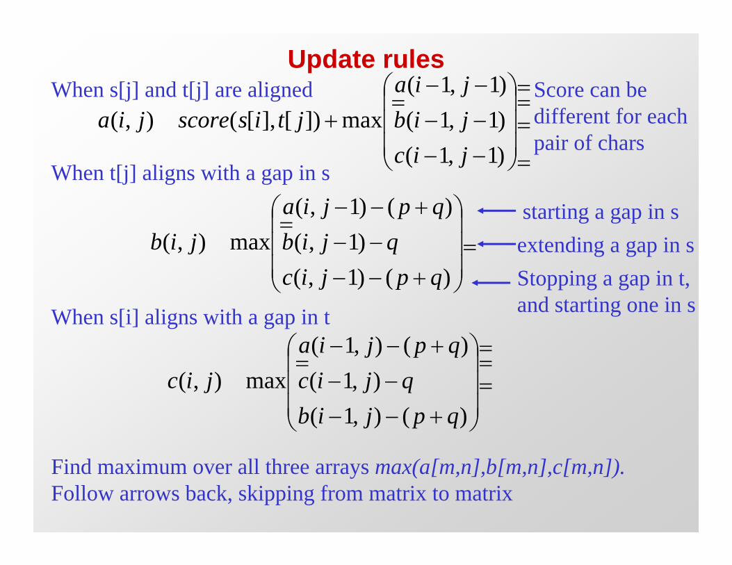
Update rulesWhen s[j] and t[j] are aligned § i a � ,1 j �1)· Score can be¨
(¸
( ( [ t j (i a , j) i s score ], [ ]) �max i b � ,1 j �1) different for each
¨ ¸ pair of chars(i c � ,1 j �1) © ¹
When t[j] aligns with a gap in s
§ i a , j �1) � ( p q)·� starting a gap in s¨ (
¸( (i b , j) max¨ i b , j �1) � q ¸ extending a gap in s
¨ ¸i c , j �1) � ( p q)( � Stopping a gap in t,© ¹and starting one in s
When s[i] aligns with a gap in t
§ i a �1 ) � ( p q)· , j �¨
(¸
( ( , ji c , j) max i c �1 ) � q ¸ ¨ ¸( , j �i b �1 ) � ( p q)© ¹
Find maximum over all three arrays max(a[m,n],b[m,n],c[m,n]).
Follow arrows back, skipping from matrix to matrix

Simplified rules
• Transitions from b to c are not necessary...
…if the worst mismatch costs less than p+q
ACC-GGTA ACCGGTAA--TGGTA A-TGGTA
¨ (When s[j] and t[j] are aligned § i a � ,1 j �1)· Score can be¸
( [ ], (i a , j ) score ( t i s [ j ]) �max¨ i b � ,1 j �1) different for each
¨ ¸ pair of chars(© i c � ,1 j �1) ¹
When t[j] aligns with a gap in s
(i b ( , j ) max¨
§ i a , j �1) � ( p � q )· starting a gap in s ¸ ¨ ¸© i b , j �1) � q( extending a gap in s¹
When s[i] aligns with a gap in t
(i c ( , j ) max¨
§ i a � ,1 j ) � ( p � q )· ¸ ¨ ¸
© i c � ,1 j ) � q( ¹

General Gap Penalty
• Gap penalties are limited by the amount of state
– Affine gap penalty: w(k) = k*p
• State: Current index tells if in a gap or not
– Linear gap penalty: w(k) = p + q*k, where q<p
• State: add binary value for each sequence: starting a gap or not
– What about quadriatic: w(k) = p+q*k+rk2.
• State: needs to encode the length of the gap, which can be O(n)
• To encode it we need O(log n) bits of information. Not feasible
– What about a (mod 3) gap penalty for protein alignments
• Gaps of length divisible by 3 are penalized less: conserve frame
• This is feasible, but requires more possible states
• Possible states are: starting, mod 3=1, mod 3=2, mod 3=0

Sequence alignment
Global Alignment
Semi-Global
Local Alignment
Linear Gap Penalty
Variations on the Theme
Dynamic Programming

Dynamic Programming Versatility
• Unified framework
– Dynamic programming algorithm. Local updates.
– Re-using past results in future computations.
– Memory usage optimizations
• Tools in our disposition
– Global alignment: entire length of two orthologous genes
– Semi-global alignment: piece of a larger sequence aligned entirely
– Local alignment: two genes sharing a functional domain
– Linear Gap Penalty: penalize first gap more than subsequent gaps
– Edit distance, min # of edit operations. M=0, m=g=-1, every operation subtracts 1, be it mutation or gap
– Longest common subsequence: M=1, m=g=0. Every match adds one, be it contiguous or not with previous.

DP Algorithm Variations
t
s
t
s
t
s
- A G T
A
A
G
C
- 0 -2 -4 -6
-2 1 -1 -1
-4 -1 -1 -2
-6 -1 0 0
-8 -3 0 -1
Global Alignment
Semi-Global Alignment
Local Alignment
- A G T
A
A
G
C
- 0 -2 -4 -6
0 1 -1 -1
0 1 0 -2
0 -1 2 1
0 -1 0 0
- A G T
A
A
G
A
- 0 0 0 0
0 1 0 0
0 1 0 0
0 0 2 0
0 1 0 1

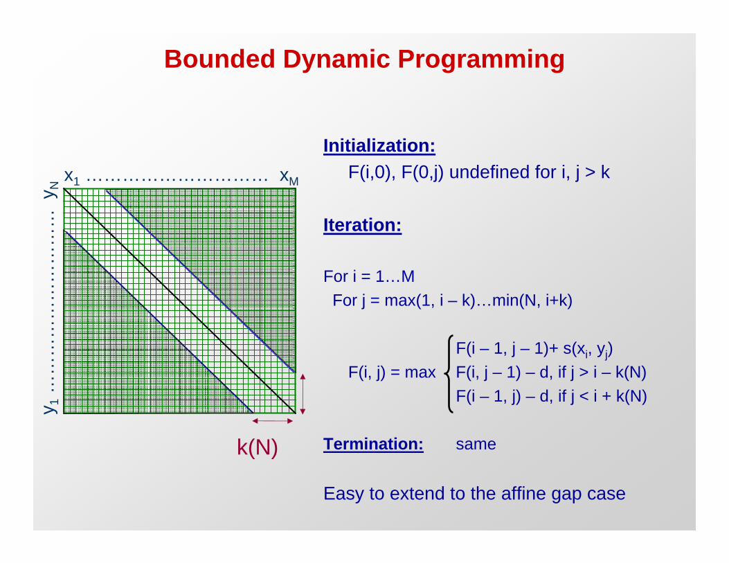
Bounded Dynamic Programming
Initialization:
F(i,0), F(0,j) undefined for i, j > k
Iteration:
For i = 1…M
For j = max(1, i – k)…min(N, i+k)
F(i – 1, j – 1)+ s(xi, yj)
F(i, j) = max F(i, j – 1) – d, if j > i – k(N)
F(i – 1, j) – d, if j < i + k(N)
Termination: same
Easy to extend to the affine gap case
x1 ………………………… xM
y1
……
……
……
……
……
yN
k(N)

Linear-space alignment
• Now, we can find k* maximizing F(M/2, k) + Fr(M/2, N-k)
• Also, we can trace the path exiting column M/2 from k*
k*
k*

Linear-Space Alignment

Hirschberg’s algorithm
• Longest common subsequence
– Given sequences s = s1 s2 … s , t = t1 t2 … tn,m
– Find longest common subsequence u = u1 … uk
• Algorithm: F(i-1, j)
• F(i, j) = max F(i, j-1)
F(i-1, j-1) + [1, if s = tj; 0 otherwise] i
• Hirschberg’s algorithm solves this in linear space
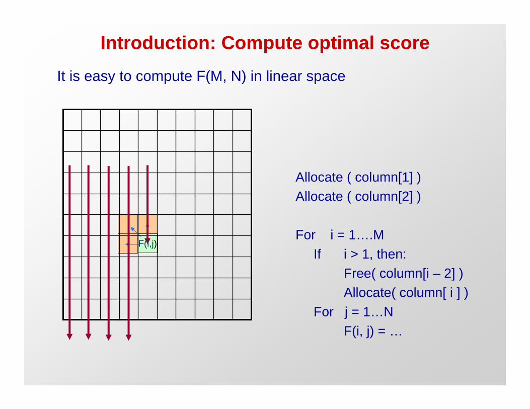
Introduction: Compute optimal score
It is easy to compute F(M, N) in linear space
F(i,j)
Allocate ( column[1] )
Allocate ( column[2] )
For i = 1….M
If i > 1, then:
Free( column[i – 2] )
Allocate( column[ i ] )
For j = 1…N
F(i, j) = …

Linear-space alignment
To compute both the optimal score and the optimal alignment:
Divide & Conquer approach:
Notation:
rx , yr: reverse of x, y
E.g. x = accgg; rx = ggcca
r rFr(i, j): optimal score of aligning xr1…x & yr
1…y ji
same as F(M-i+1, N-j+1)

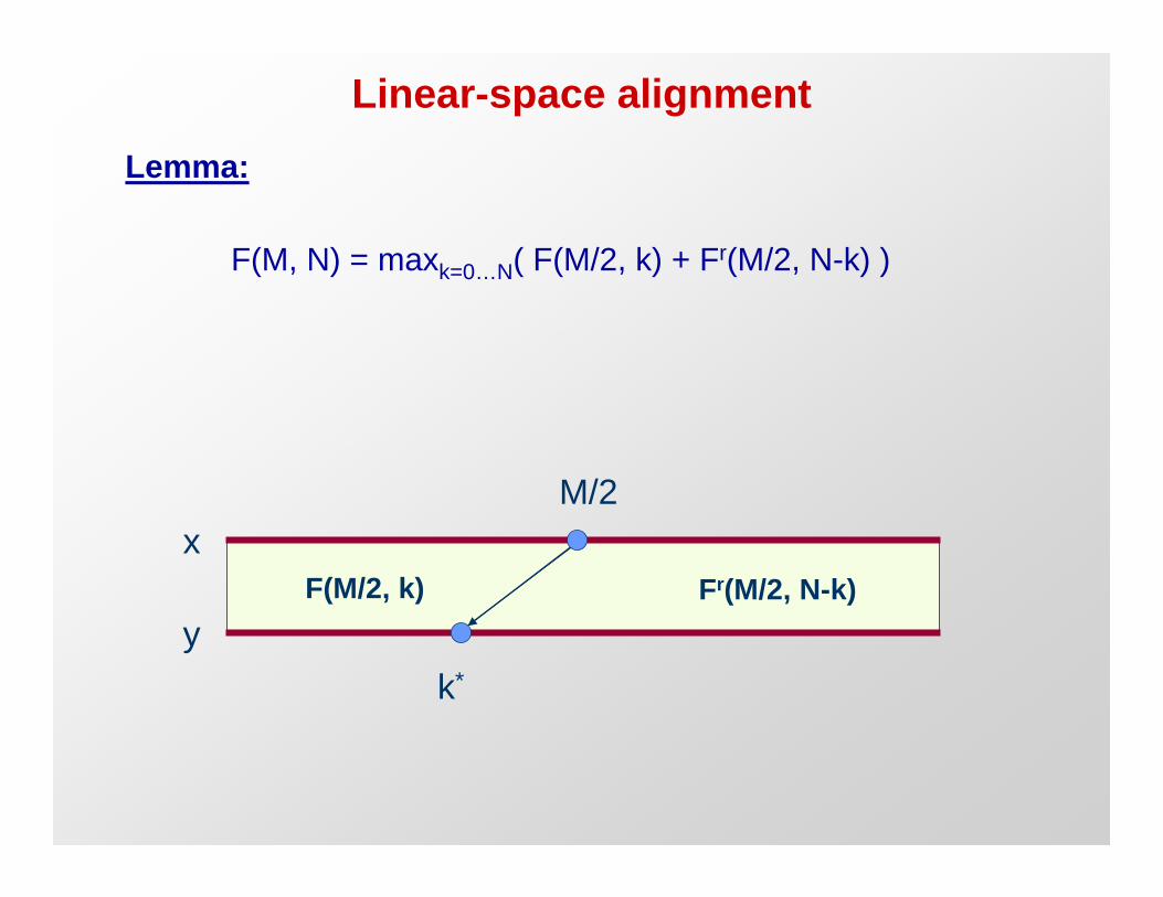
Linear-space alignment
Lemma:
F(M, N) = maxk=0…N( F(M/2, k) + Fr(M/2, N-k) )
x
y
M/2
k*
Fr(M/2, N-k)F(M/2, k)

Linear-space alignment
• Now, using 2 columns of space, we can compute
for k = 1…M, F(M/2, k), Fr(M/2, N-k)
PLUS the backpointers

Linear-space alignment
• Now, we can find k* maximizing F(M/2, k) + Fr(M/2, N-k)
• Also, we can trace the path exiting column M/2 from k*
k*
k*

Linear-space alignment
• Iterate this procedure to the left and right!
k*
N-k*
M/2 M/2

Linear-space alignment
Hirschberg’s Linear-space algorithm:
MEMALIGN(l, l’, r, r’): (aligns x …xl’ with yr…yr’)l
1. Let h = ª(l’-l)/2º 2. Find in Time O((l’ – l) u (r’-r)), Space O(r’-r)
the optimal path, Lh, entering column h-1, exiting column h
Let k1 = pos’n at column h – 2 where Lh enters
k2 = pos’n at column h + 1 where Lh exits
3. MEMALIGN(l, h-2, r, k1)
4. Output Lh
5. MEMALIGN(h+1, l’, k2, r’)
Top level call: MEMALIGN(1, M, 1, N)

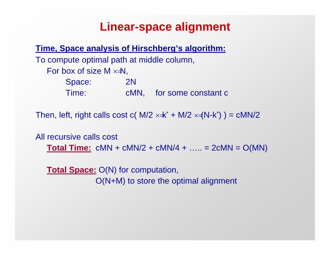
Linear-space alignment
Time, Space analysis of Hirschberg’s algorithm:
To compute optimal path at middle column,
For box of size M u N,
Space: 2N
Time: cMN, for some constant c
Then, left, right calls cost c( M/2 u k* + M/2 u (N-k*) ) = cMN/2
All recursive calls cost
Total Time: cMN + cMN/2 + cMN/4 + ….. = 2cMN = O(MN)
Total Space: O(N) for computation,
O(N+M) to store the optimal alignment

The Four-Russian Algorithm
A useful speedup of Dynamic Programming

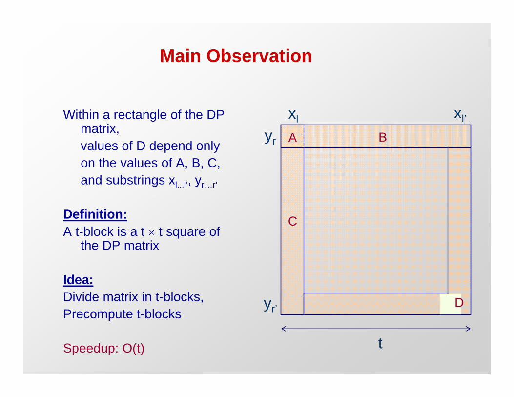
Main Observation
Within a rectangle of the DP matrix,
values of D depend only
on the values of A, B, C,
and substrings xl...l’, yr…r’
Definition:
A t-block is a t u t square of the DP matrix
Idea:
Divide matrix in t-blocks,
Precompute t-blocks
Speedup: O(t)
A B
C
D
xl xl’
yr
yr’
t

The Four-Russian Algorithm
Main structure of the algorithm:
• Divide NuN DP matrix into KuKlog2N-blocks that overlap by 1 column & 1 row
• For i = 1……K
• For j = 1……K
• Compute Di,j as a function of
Ai,j, Bi,j, Ci,j, x[li…l’i], y[rj…r’j]
Time: O(N2 / log2N)
times the cost of step 4
t t t

The Four-Russian Algorithm
Another observation:
( Assume m = 0, s = 1, d = 1 )
Lemma. Two adjacent cells of F(.,.) differ by at most 1
Gusfield’s book covers case where m = 0,
called the edit distance (p. 216):
minimum # of substitutions + gaps to transform one string to another

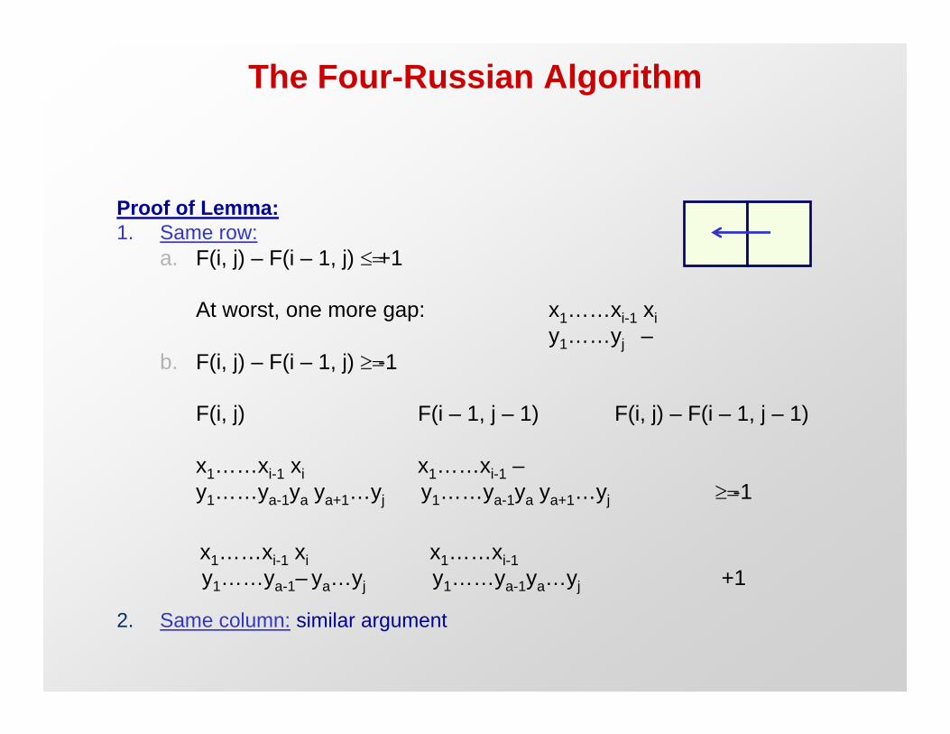
The Four-Russian Algorithm
Proof of Lemma:
1. Same row:
a. F(i, j) – F(i – 1, j) d +1
At worst, one more gap: x1……xi-1 xi
y1……yj –
b. F(i, j) – F(i – 1, j) t -1
F(i, j) F(i – 1, j – 1) F(i, j) – F(i – 1, j – 1)
x ……x x x1……x – 1 i-1 i i-1
y1……ya-1ya ya+1…yj y1……ya-1ya ya+1…yj t -1
x1……x x x ……xi-1 i 1 i-1
y1……ya-1– ya…yj y1……ya-1ya…yj +1
2. Same column: similar argument
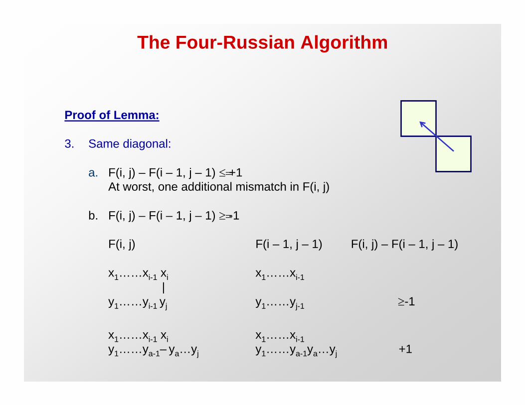
The Four-Russian Algorithm
Proof of Lemma:
3. Same diagonal:
a. F(i, j) – F(i – 1, j – 1) d +1
At worst, one additional mismatch in F(i, j)
b. F(i, j) – F(i – 1, j – 1) t -1
F(i, j)
x1……x xi-1 i
|
y1……yi-1 yj
x1……x xi-1 i
y1……ya-1– ya…yj
F(i – 1, j – 1)
x ……x1 i-1
y1……yj-1
x ……x1 i-1
y1……ya-1ya…yj
F(i, j) – F(i – 1, j – 1)
t-1
+1

The Four-Russian Algorithm
Definition:
The offset vector is a
t-long vector of values
from {-1, 0, 1},
where the first entry is 0
If we know the value at A,
and the top row, left column
offset vectors,
and xl……xl’, yr……yr’,
Then we can find D
A B
C
D
xl xl’
yr
yr’
t

The Four-Russian Algorithm
Example:
x = AACT
y = CACT
5655
6554
5655
4565A A C T
C
A
C
T
0 1 -1
0
0
-1
1
0 0 1 -1
0
1
1
-1
-1
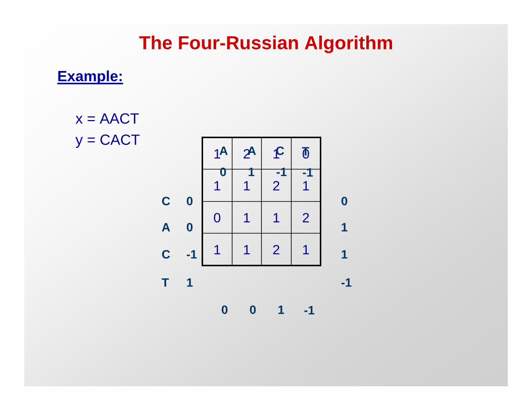
The Four-Russian Algorithm
Example:
x = AACT
y = CACT
1211
2110
1211
0121A A C T
C
A
C
T
0 1 -1
0
0
-1
1
0 0 1 -1
0
1
1
-1
-1

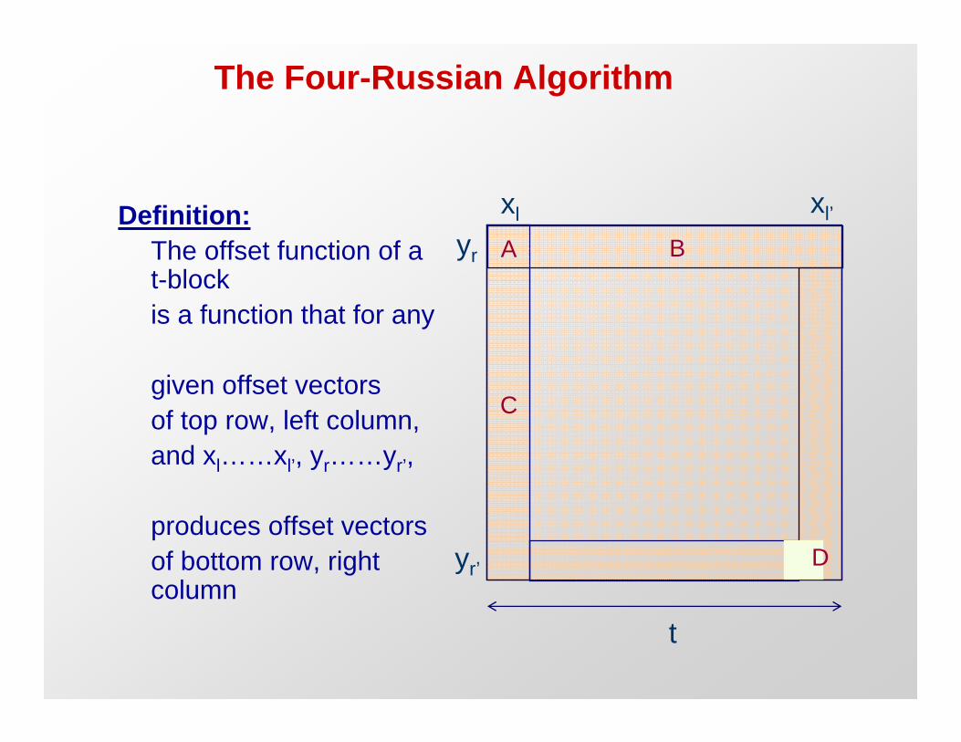
The Four-Russian Algorithm
Definition:
The offset function of a t-block
is a function that for any
given offset vectors
of top row, left column,
and xl……xl’, yr……yr’,
produces offset vectors
of bottom row, right column
A B
C
D
xl xl’
yr
yr’
t

The Four-Russian Algorithm
4
3
We can pre-compute the offset function:
2(t-1) possible input offset vectors
2t possible strings x ……xl’, yr……yr’l
Therefore 32(t-1) u 42t values to pre-compute
We can keep all these values in a table, and look up in linear time,
or in O(1) time if we assume
constant-lookup RAM for log-sized inputs

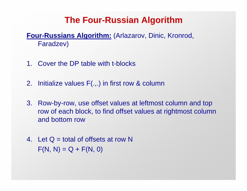
The Four-Russian Algorithm
Four-Russians Algorithm: (Arlazarov, Dinic, Kronrod,
Faradzev)
1. Cover the DP table with t-blocks
2. Initialize values F(.,.) in first row & column
3. Row-by-row, use offset values at leftmost column and top
row of each block, to find offset values at rightmost column
and bottom row
4. Let Q = total of offsets at row N
F(N, N) = Q + F(N, 0)

The Four-Russian Algorithm
t t t
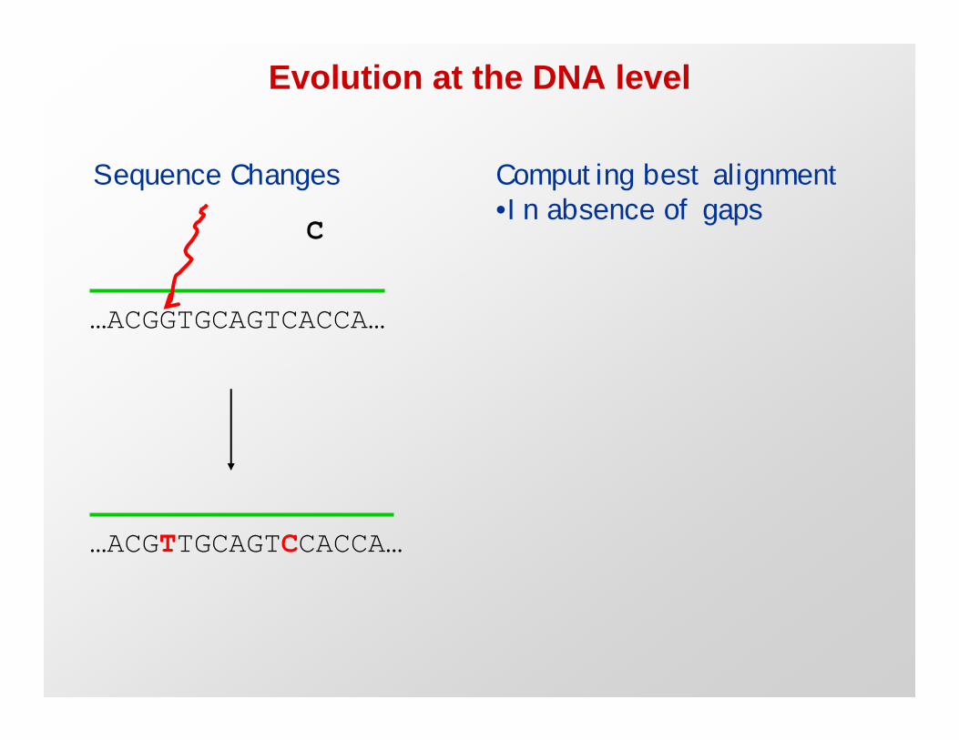
Evolution at the DNA level
…ACGGTGCAGTCACCA…
…ACGTTGCAGTCCACCA…
C
Sequence Changes Computing best alignment •In absence of gaps

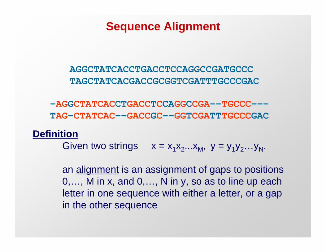
Sequence Alignment
AGGCTATCACCTGACCTCCAGGCCGATGCCCTAGCTATCACGACCGCGGTCGATTTGCCCGAC
-AGGCTATCACCTGACCTCCAGGCCGA--TGCCC---TAG-CTATCAC--GACCGC--GGTCGATTTGCCCGAC
Definition
Given two strings x = x1x2...xM, y = y1y2…yN,
an alignment is an assignment of gaps to positions
0,…, M in x, and 0,…, N in y, so as to line up each
letter in one sequence with either a letter, or a gap
in the other sequence

Scoring Function
• Sequence edits:
AGGCCTC
– Mutations
AGGACTC
– Insertions
AGGGCCTC
– Deletions
AGG.CTC
Scoring Function:
Match: +m
Mismatch: -s
Gap: -d
Score F = (# matches) u m - (# mismatches) u s – (#gaps) u d

How do we compute the best alignment?
AGTGACCTGGGAAGACCCTGACCCTGGGTCACAAAACTC
AGTGCCCTGGAACCCTGACGGTGGGTCACAAAACTTCTGGA
Too many possible alignments:
O( 2M+N)
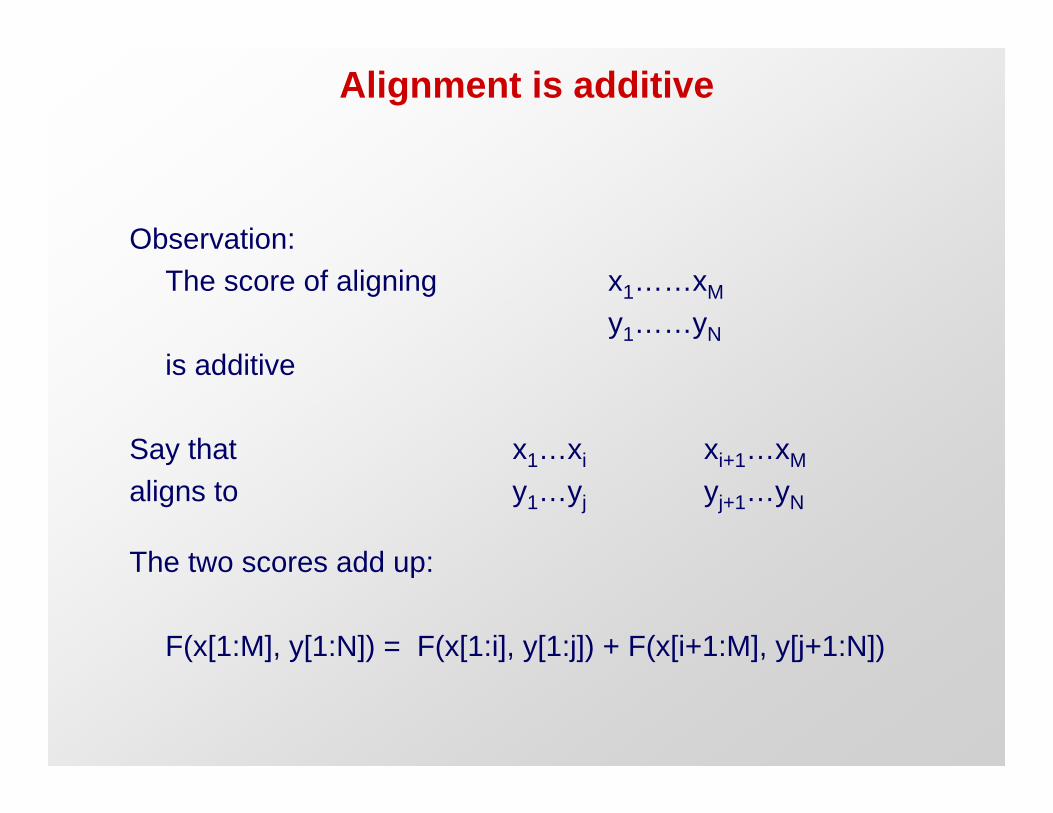
Alignment is additive
Observation:
The score of aligning x1……xM
y1……yN
is additive
Say that x1…xi xi+1…xM
aligns to y1…yj yj+1…yN
The two scores add up:
F(x[1:M], y[1:N]) = F(x[1:i], y[1:j]) + F(x[i+1:M], y[j+1:N])

Dynamic Programming
• We will now describe a dynamic programming
algorithm
Suppose we wish to align
x1……xM
y1……yN
Let
F(i,j) = optimal score of aligning
x1……xi
y1……yj
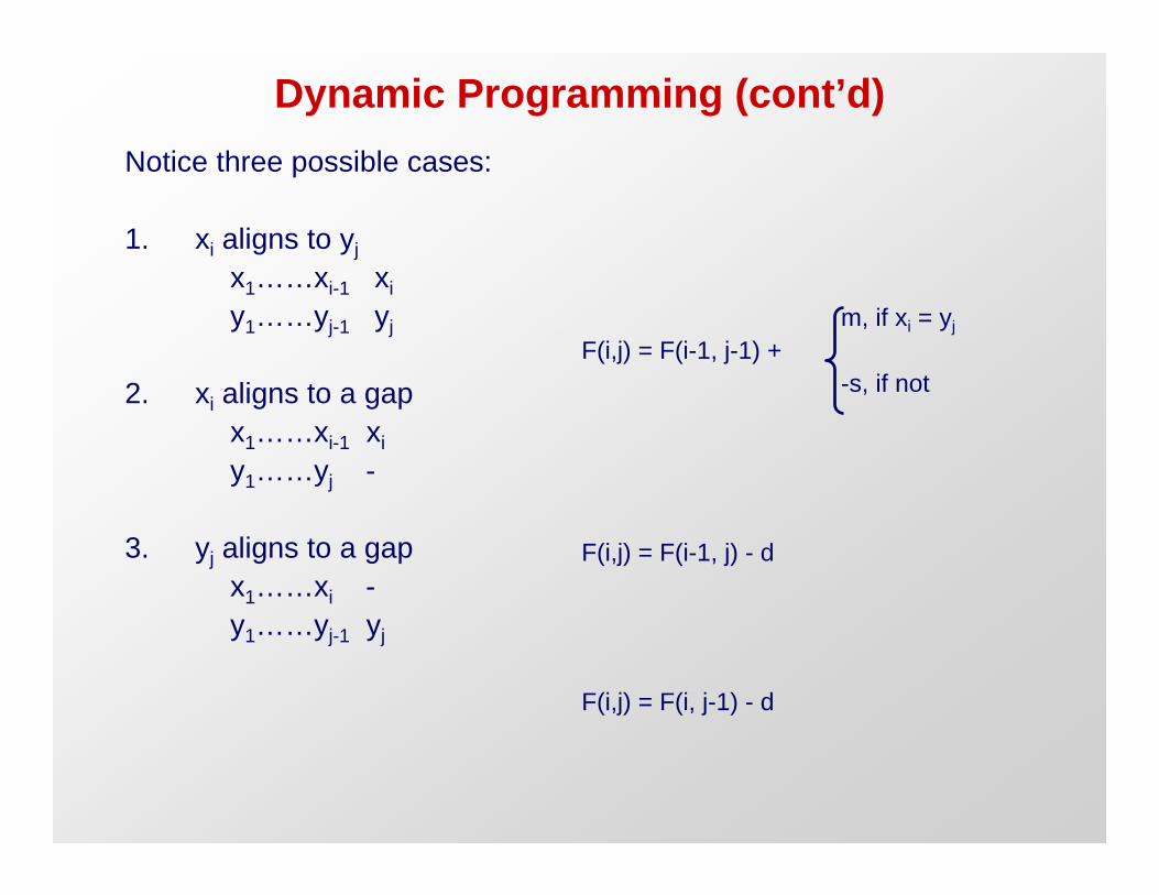
Dynamic Programming (cont’d)
Notice three possible cases:
1. xi aligns to yj
x1……xi-1 xi
y1……yj-1 yj m, if xi = y
-s, if not
j
F(i,j) = F(i-1, j-1) +
2. xialigns to a gap
x1……xi-1 xi
y1……yj
3. yj aligns to a gap F(i,j) = F(i-1, j) - d
x1……x i
y1……yj-1 yj
F(i,j) = F(i, j-1) - d

Dynamic Programming (cont’d)
• How do we know which case is correct?
Inductive assumption:
F(i, j-1), F(i-1, j), F(i-1, j-1) are optimal
Then,
F(i-1, j-1) + s(x , yj)
F(i, j) = max i
F(i-1, j) – d
F( i, j-1) – d
Where s(x , yj) = m, if x = y ; -s, if noti i j

Example
x = AGTA
y = ATA
F(i,j) i = 0 1 2 3 4
j = 0
1
2
3
A G T A
0 -1 -2 -3 -4
A -1 1 0 -1 -2
T -2 0 0 1 0
A -3 -1 -1 0 2
m = 1
s = -1
d = -1
Optimal Alignment:
F(4,3) = 2
AGTA
A - TA

The Needleman-Wunsch Matrix
y1
……
……
……
……
……
……
y
N
x1 ……………………………… xM
Every nondecreasing
path
from (0,0) to (M, N)
corresponds to
an alignment
of the two sequences
Can think of it as a
divide-and-conquer algorithm

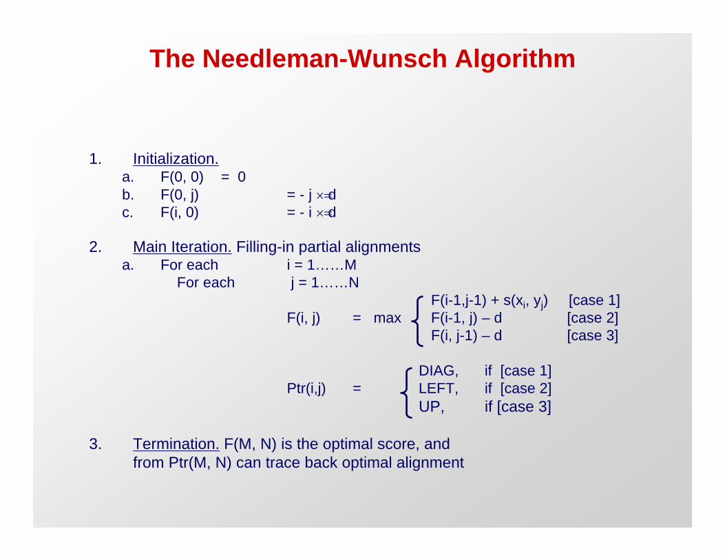
The Needleman-Wunsch Algorithm
1. Initialization. a. F(0, 0) = 0
b. F(0, j) = - j u d
c. F(i, 0) = - i u d
2. Main Iteration. Filling-in partial alignments a. For each i = 1……M
For each j = 1……N
F(i-1,j-1) + s(x , yj)i
F(i, j) = max F(i-1, j) – d
F(i, j-1) – d
DIAG, if [case 1]
Ptr(i,j) = LEFT, if [case 2]
UP, if [case 3]
3. Termination. F(M, N) is the optimal score, and
from Ptr(M, N) can trace back optimal alignment
[case 1]
[case 2]
[case 3]

Performance
O(NM)
O(NM)
•
me:
Later we will cover more efficient methods
• Ti
• Space:

A variant of the basic algorithm:
• Maybe it is OK to have an unlimited # of gaps in
the beginning and end:
----------CTATCACCTGACCTCCAGGCCGATGCCCCTTCCGGCGCGAGTTCATCTATCAC--GACCGC--GGTCG--------------
• Then, we don’t want to penalize gaps in the ends

Different types of overlaps

The Overlap Detection variant
Changes:
1. Initializationx1 ……………………………… xM
y 1
……
……
……
……
……
……
y
N For all i, j,
F(i, 0) = 0
F(0, j) = 0
2. Termination
maxi F(i, N)
FOPT = max max F(M,j
j)

The local alignment problem
Given two strings x = x1……xM,
y = y1……yN
(optimal global alignment value)
is maximum
e.g. x = aaaacccccgggg
y = cccgggaaccaacc
Find substrings x’, y’ whose similarity

Why local alignment
• Genes are shuffled between genomes
• Portions of proteins (domains) are often conserved
Image removed due to copyright restrictions.

Cross-species genome similarity
• 98% of genes are conserved between any two mammals
• >70% average similarity in protein sequence
hum_a : GTTGACAATAGAGGGTCTGGCAGAGGCTC--------------------- @ 57331/400001 mus_a : GCTGACAATAGAGGGGCTGGCAGAGGCTC--------------------- @ 78560/400001 rat_a : GCTGACAATAGAGGGGCTGGCAGAGACTC--------------------- @ 112658/369938 fug_a : TTTGTTGATGGGGAGCGTGCATTAATTTCAGGCTATTGTTAACAGGCTCG @ 36008/68174
hum_a : CTGGCCGCGGTGCGGAGCGTCTGGAGCGGAGCACGCGCTGTCAGCTGGTG @ 57381/400001 mus_a : CTGGCCCCGGTGCGGAGCGTCTGGAGCGGAGCACGCGCTGTCAGCTGGTG @ 78610/400001 rat_a : CTGGCCCCGGTGCGGAGCGTCTGGAGCGGAGCACGCGCTGTCAGCTGGTG @ 112708/369938 “atoh” enhancer in fug_a : TGGGCCGAGGTGTTGGATGGCCTGAGTGAAGCACGCGCTGTCAGCTGGCG @ 36058/68174
human, mouse, hum_a : AGCGCACTCTCCTTTCAGGCAGCTCCCCGGGGAGCTGTGCGGCCACATTT @ 57431/400001 rat, fugu fishmus_a : AGCGCACTCG-CTTTCAGGCCGCTCCCCGGGGAGCTGAGCGGCCACATTT @ 78659/400001 rat_a : AGCGCACTCG-CTTTCAGGCCGCTCCCCGGGGAGCTGCGCGGCCACATTT @ 112757/369938 fug_a : AGCGCTCGCG------------------------AGTCCCTGCCGTGTCC @ 36084/68174
hum_a : AACACCATCATCACCCCTCCCCGGCCTCCTCAACCTCGGCCTCCTCCTCG @ 57481/400001 mus_a : AACACCGTCGTCA-CCCTCCCCGGCCTCCTCAACCTCGGCCTCCTCCTCG @ 78708/400001 rat_a : AACACCGTCGTCA-CCCTCCCCGGCCTCCTCAACCTCGGCCTCCTCCTCG @ 112806/369938 fug_a : CCGAGGACCCTGA------------------------------------- @ 36097/68174

The Smith-Waterman algorithm
Idea: Ignore badly aligning regions
Modifications to Needleman-Wunsch:
Initialization: F(0, j) = F(i, 0) = 0
0
Iteration: F(i, j) = max F(i – 1, j) – d
F(i, j – 1) – d
F(i – 1, j – 1) + s(x , yj)i
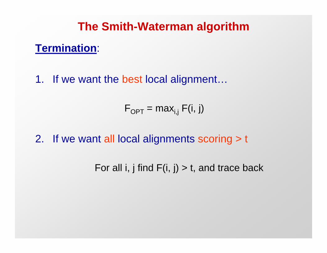
The Smith-Waterman algorithm
Termination:
1. If we want the best local alignment…
FOPT = maxi,j F(i, j)
2. If we want all local alignments scoring > t
For all i, j find F(i, j) > t, and trace back

Scoring the gaps more accurately
Current model:
J(n)Gap of length n
incurs penalty nud
However, gaps usually occur in bunches
Convex gap penalty function:
J(n):
for all n, J(n + 1) - J(n) d J(n) - J(n – 1) J(n)

General gap dynamic programming
Initialization: same
Iteration:
F(i-1, j-1) + s(xi, yj)
F(i, j) = max
max
maxk=0…i-1F(k,j) – J(i-k)
k=0…j-1F(i,k) – J(j-k)
Termination: same
Running Time: O(N2M)
Space:
(assume N>M)
O(NM)
Compromise: affine gaps
J(n) = d + (n – 1)ue
| | J(n) gap gap
open extend
d To compute optimal alignment,
e
At position i,j, need to “remember” best score if gap is open
best score if gap is not open
F(i, j): score of alignment x1…x to y1…yji
ifif xi aligns to yj
G(i, j): score ifif x , or yj, aligns to a gapi

Needleman-Wunsch with affine gaps
Initialization: F(i, 0) = d + (i – 1)ue
F(0, j) = d + (j – 1)ue
Iteration:
F(i – 1, j – 1) + s(x , yj)i
F(i, j) = max
G(i – 1, j – 1) + s(x , yj)i
F(i – 1, j) – d
F(i, j – 1) – d
G(i, j) = max
G(i, j – 1) – e
G(i – 1, j) – e
Termination: same
Sequence Alignment
AGGCTATCACCTGACCTCCAGGCCGATGCCCTAGCTATCACGACCGCGGTCGATTTGCCCGAC
-AGGCTATCACCTGACCTCCAGGCCGA--TGCCC---TAG-CTATCAC--GACCGC--GGTCGATTTGCCCGAC
Definition
Given two strings x = x1x2...xM, y = y1y2…yN,
an alignment is an assignment of gaps to positions
0,…, M in x, and 0,…, N in y, so as to line up each
letter in one sequence with either a letter, or a gap
in the other sequence

Scoring Function
• Sequence edits:
AGGCCTC
– Mutations
AGGACTC
– Insertions
AGGGCCTC
– Deletions
AGG.CTC
Scoring Function:
Match: +m
Mismatch: -s
Gap: -d
Score F = (# matches) u m - (# mismatches) u s – (#gaps) u d
The Needleman-Wunsch Algorithm
1. Initialization. a. F(0, 0) = 0
b. F(0, j) = - j u d
c. F(i, 0) = - i u d
2. Main Iteration. Filling-in partial alignments a. For each i = 1……M
For each j = 1……N
F(i-1,j-1) + s(x , yj)i
F(i, j) = max F(i-1, j) – d
F(i, j-1) – d
DIAG, if [case 1]
Ptr(i,j) = LEFT, if [case 2]
UP, if [case 3]
3. Termination. F(M, N) is the optimal score, and
from Ptr(M, N) can trace back optimal alignment
[case 1]
[case 2]
[case 3]

The Smith-Waterman algorithm
Idea: Ignore badly aligning regions
Modifications to Needleman-Wunsch:
Initialization: F(0, j) = F(i, 0) = 0
0
Iteration: F(i, j) = max F(i – 1, j) – d
F(i, j – 1) – d
F(i – 1, j – 1) + s(x , yj)i
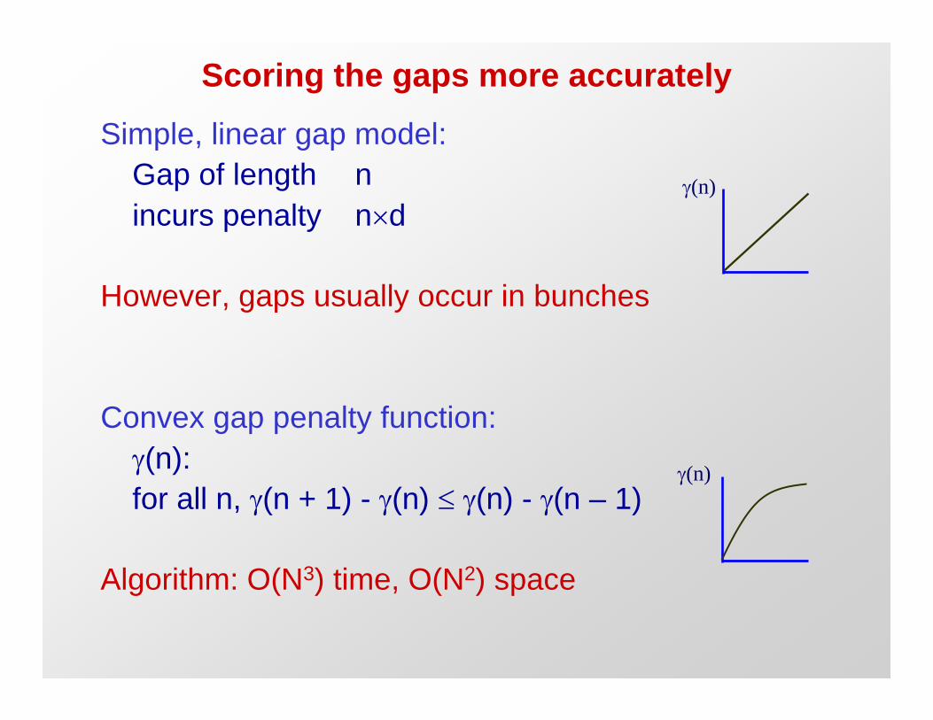
Scoring the gaps more accurately
Simple, linear gap model:
Gap of length n J(n)
incurs penalty nud
However, gaps usually occur in bunches
Convex gap penalty function:
J(n): J(n)
for all n, J(n + 1) - J(n) d J(n) - J(n – 1)
Algorithm: O(N3) time, O(N2) space

Compromise: affine gaps
J(n) = d + (n – 1)ue
| | J(n) gap gap
open extend
d To compute optimal alignment,
e
At position i,j, need to “remember” best score if gap is open
best score if gap is not open
F(i, j): score of alignment x1…x to y1…yji
ifif xi aligns to yj
G(i, j): score ifif x , or yj, aligns to a gapi

Why do we need two matrices?
• xi aligns to yj
x1……xi-1 xi xi+1
y1……yj-1 yj -
2. xi aligns to a gap
x1……xi-1 xi xi+1
y1……yj … -
Add -d
Add -e
Needleman-Wunsch with affine gaps

Needleman-Wunsch with affine gaps
Initialization: F(i, 0) = d + (i – 1)ue
F(0, j) = d + (j – 1)ue
Iteration:
F(i – 1, j – 1) + s(x , yj)i
F(i, j) = max
G(i – 1, j – 1) + s(x , yj)i
F(i – 1, j) – d
F(i, j – 1) – d
G(i, j) = max
G(i, j – 1) – e
G(i – 1, j) – e
Termination: same

To generalize a little…
… think of how you would compute optimal alignment
with this gap function
J(n)
….in time O(MN)

Bounded Dynamic Programming
Assume we know that x and y are very similar
Assumption: # gaps(x, y) < k(N) ( say N>M )
xi
Then, | implies | i – j | < k(N)
yj
We can align x and y more efficiently:
Time, Space: O(N u k(N)) << O(N2)
Bounded Dynamic Programming
Initialization:
F(i,0), F(0,j) undefined for i, j > k
Iteration:
For i = 1…M
For j = max(1, i – k)…min(N, i+k)
F(i – 1, j – 1)+ s(xi, yj)
F(i, j) = max F(i, j – 1) – d, if j > i – k(N)
F(i – 1, j) – d, if j < i + k(N)
Termination: same
Easy to extend to the affine gap case
x1 ………………………… xM
y1
……
……
……
……
……
yN
k(N)

Linear-Space Alignment

Hirschberg’s algortihm
• Longest common subsequence
– Given sequences s = s1 s2 … s , t = t1 t2 … tn,m
– Find longest common subsequence u = u1 … uk
• Algorithm: F(i-1, j)
• F(i, j) = max F(i, j-1)
F(i-1, j-1) + [1, if s = tj; 0 otherwise] i
• Hirschberg’s algorithm solves this in linear space

Introduction: Compute optimal score
It is easy to compute F(M, N) in linear space
F(i,j)
Allocate ( column[1] )
Allocate ( column[2] )
For i = 1….M
If i > 1, then:
Free( column[i – 2] )
Allocate( column[ i ] )
For j = 1…N
F(i, j) = …

Linear-space alignment
To compute both the optimal score and the optimal alignment:
Divide & Conquer approach:
Notation:
rx , yr: reverse of x, y
E.g. x = accgg; rx = ggcca
r rFr(i, j): optimal score of aligning xr1…x & yr
1…y ji
same as F(M-i+1, N-j+1)
Linear-space alignment
Lemma:
F(M, N) = maxk=0…N( F(M/2, k) + Fr(M/2, N-k) )
x
y
M/2
k*
Fr(M/2, N-k)F(M/2, k)

Linear-space alignment
• Now, using 2 columns of space, we can compute
for k = 1…M, F(M/2, k), Fr(M/2, N-k)
PLUS the backpointers

Linear-space alignment
• Now, we can find k* maximizing F(M/2, k) + Fr(M/2, N-k)
• Also, we can trace the path exiting column M/2 from k*
k*
k*

Linear-space alignment
• Iterate this procedure to the left and right!
k*
N-k*
M/2 M/2

Linear-space alignment
Hirschberg’s Linear-space algorithm:
MEMALIGN(l, l’, r, r’): (aligns x …xl’ with yr…yr’)l
1. Let h = ª(l’-l)/2º 2. Find in Time O((l’ – l) u (r’-r)), Space O(r’-r)
the optimal path, Lh, entering column h-1, exiting column h
Let k1 = pos’n at column h – 2 where Lh enters
k2 = pos’n at column h + 1 where Lh exits
3. MEMALIGN(l, h-2, r, k1)
4. Output Lh
5. MEMALIGN(h+1, l’, k2, r’)
Top level call: MEMALIGN(1, M, 1, N)
Linear-space alignment
Time, Space analysis of Hirschberg’s algorithm:
To compute optimal path at middle column,
For box of size M u N,
Space: 2N
Time: cMN, for some constant c
Then, left, right calls cost c( M/2 u k* + M/2 u (N-k*) ) = cMN/2
All recursive calls cost
Total Time: cMN + cMN/2 + cMN/4 + ….. = 2cMN = O(MN)
Total Space: O(N) for computation,
O(N+M) to store the optimal alignment

The Four-Russian Algorithm
A useful speedup of Dynamic Programming
Main Observation
Within a rectangle of the DP matrix,
values of D depend only
on the values of A, B, C,
and substrings xl...l’, yr…r’
Definition:
A t-block is a t u t square of the DP matrix
Idea:
Divide matrix in t-blocks,
Precompute t-blocks
Speedup: O(t)
A B
C
D
xl xl’
yr
yr’
t

The Four-Russian Algorithm
Main structure of the algorithm:
• Divide NuN DP matrix into KuKlog2N-blocks that overlap by 1 column & 1 row
• For i = 1……K
• For j = 1……K
• Compute Di,j as a function of
Ai,j, Bi,j, Ci,j, x[li…l’i], y[rj…r’j]
Time: O(N2 / log2N)
times the cost of step 4
t t t

The Four-Russian Algorithm
Another observation:
( Assume m = 0, s = 1, d = 1 )
Lemma. Two adjacent cells of F(.,.) differ by at most 1
Gusfield’s book covers case where m = 0,
called the edit distance (p. 216):
minimum # of substitutions + gaps to transform one string to another
The Four-Russian Algorithm
Proof of Lemma:
1. Same row:
a. F(i, j) – F(i – 1, j) d +1
At worst, one more gap: x1……xi-1 xi
y1……yj –
b. F(i, j) – F(i – 1, j) t -1
F(i, j) F(i – 1, j – 1) F(i, j) – F(i – 1, j – 1)
x ……x x x1……x – 1 i-1 i i-1
y1……ya-1ya ya+1…yj y1……ya-1ya ya+1…yj t -1
x1……x x x ……xi-1 i 1 i-1
y1……ya-1– ya…yj y1……ya-1ya…yj +1
2. Same column: similar argument

The Four-Russian Algorithm
Proof of Lemma:
3. Same diagonal:
a. F(i, j) – F(i – 1, j – 1) d +1
At worst, one additional mismatch in F(i, j)
b. F(i, j) – F(i – 1, j – 1) t -1
F(i, j)
x1……x xi-1 i
|
y1……yi-1 yj
x1……x xi-1 i
y1……ya-1– ya…yj
F(i – 1, j – 1)
x ……x1 i-1
y1……yj-1
x ……x1 i-1
y1……ya-1ya…yj
F(i, j) – F(i – 1, j – 1)
t-1
+1

The Four-Russian Algorithm
Definition:
The offset vector is a
t-long vector of values
from {-1, 0, 1},
where the first entry is 0
If we know the value at A,
and the top row, left column
offset vectors,
and xl……xl’, yr……yr’,
Then we can find D
A B
C
D
xl xl’
yr
yr’
t

The Four-Russian Algorithm
Example:
x = AACT
y = CACT
5655
6554
5655
4565A A C T
C
A
C
T
0 1 -1
0
0
-1
1
0 0 1 -1
0
1
1
-1
-1

The Four-Russian Algorithm
Example:
x = AACT
y = CACT
1211
2110
1211
0121A A C T
C
A
C
T
0 1 -1
0
0
-1
1
0 0 1 -1
0
1
1
-1
-1
The Four-Russian Algorithm
Definition:
The offset function of a t-block
is a function that for any
given offset vectors
of top row, left column,
and xl……xl’, yr……yr’,
produces offset vectors
of bottom row, right column
A B
C
D
xl xl’
yr
yr’
t

The Four-Russian Algorithm
4
3
We can pre-compute the offset function:
2(t-1) possible input offset vectors
2t possible strings x ……xl’, yr……yr’l
Therefore 32(t-1) u 42t values to pre-compute
We can keep all these values in a table, and look up in linear time,
or in O(1) time if we assume
constant-lookup RAM for log-sized inputs
The Four-Russian Algorithm
Four-Russians Algorithm: (Arlazarov, Dinic, Kronrod,
Faradzev)
1. Cover the DP table with t-blocks
2. Initialize values F(.,.) in first row & column
3. Row-by-row, use offset values at leftmost column and top
row of each block, to find offset values at rightmost column
and bottom row
4. Let Q = total of offsets at row N
F(N, N) = Q + F(N, 0)

The Four-Russian Algorithm
t t t