Lecture 4- Cosmological parameter dependence of the temperature power spectrum (continued)

- Polarisation

Planck Collaboration (2016)

Sachs-Wolfe Sound Wave

Let’s understand the peak heights

Silk+Landau Damping

` ⇡ 302⇥ qrs/⇡

Not quite there yet…• The first peak is too low

• We need to include the “integrated Sachs-Wolfe effect”

•How to fill zeros between the peaks?

• We need to include the Doppler shift of light

Doppler Shift of Light

• Using the velocity potential, we write Line-of-sight direction

Coming distance (r)

vB is the bulk velocity of a baryon fluid

�n̂ ·r�uB/a

• In tight coupling,

• Using energy conservation,

Doppler Shift of Light

• Using the velocity potential, we write

vB is the bulk velocity of a baryon fluid

�n̂ ·r�uB/a

• In tight coupling,

• Using energy conservation,

Velocity potential is a time-derivative

of the energy density:

cos(qrs) becomes sin(qrs)!

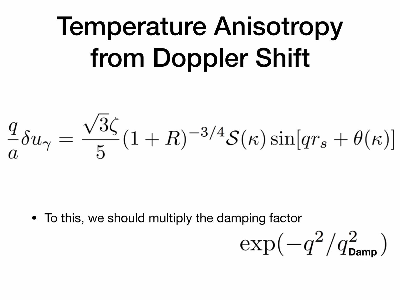
Temperature Anisotropy from Doppler Shift

• To this, we should multiply the damping factor

Damp

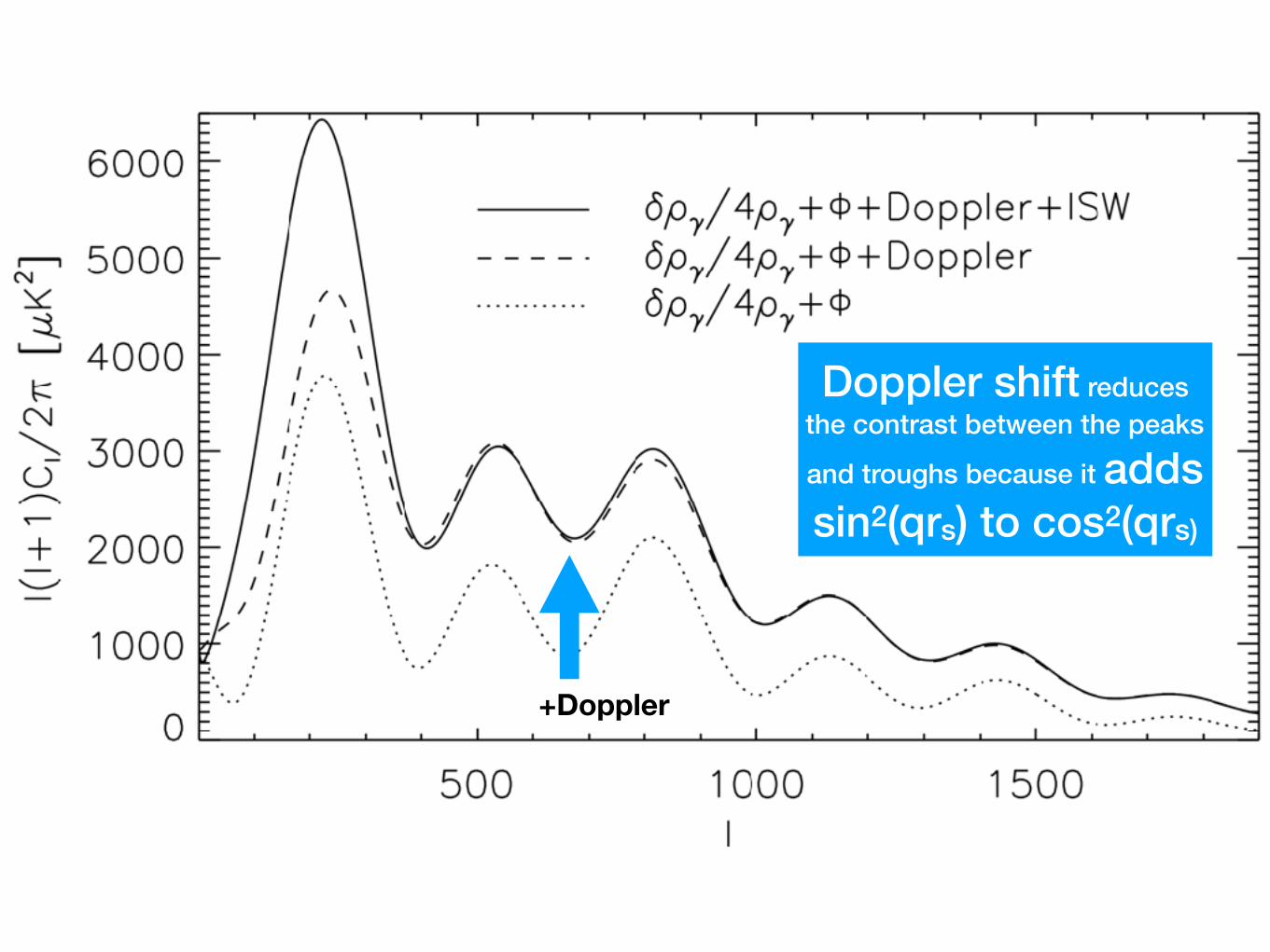
+Doppler

Doppler shift reduces the contrast between the peaks

and troughs because it adds sin2(qrs) to cos2(qrs)

(Early) ISWHu & Sugiyama (1996)

“integrated Sachs-Wolfe” (ISW) effect

Gravitational potentials still decay after last-scattering because the Universe then was not completely matter-dominated yet

+Doppler

+ISW

Early ISW affects only the first peak because it occurs after

the last-scattering epoch, subtending a larger angle.

Not only it boosts the first peak, but also it makes it “fatter”

We are ready!

• We are ready to understand the effects of all the cosmological parameters.

• Let’s start with the baryon density

The sound horizon, rs, changes when the baryon density changes, resulting in a shift in the peak positions.

Adjusting it makes the physical effect at the last scattering manifest

Zero-point shift of the oscillations

Zero-point shift effect compensated by (1+R)–1/4 and

Silk damping

Less tight coupling: Enhanced Silk damping for low baryon density

Total Matter Density

Total Matter Density

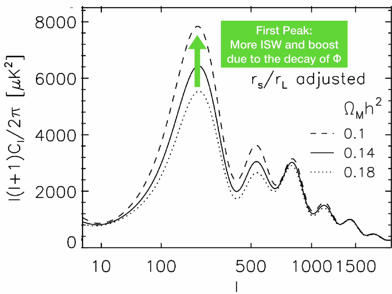
Total Matter DensityFirst Peak: More ISW and boost due to the decay of Φ

Total Matter Density2nd, 3rd, 4th Peaks: Boosts due to the

decay of Φ

Less and less effects at larger multipoles

Effects of Relativistic Neutrinos

• To see the effects of relativistic neutrinos, we artificially increase the number of neutrino species from 3 to 7

• Great energy density in neutrinos, i.e., greater energy density in radiation

• Longer radiation domination -> More ISW and boosts due to potential decay(1)

After correcting for more ISW and boosts due to

potential decay

(2): Viscosity Effect on the Amplitude of Sound Waves

The solution is

where

Hu & Sugiyama (1996)

Bashinsky & Seljak (2004)

Phase shift!

After correcting for the viscosity effect on the

amplitude

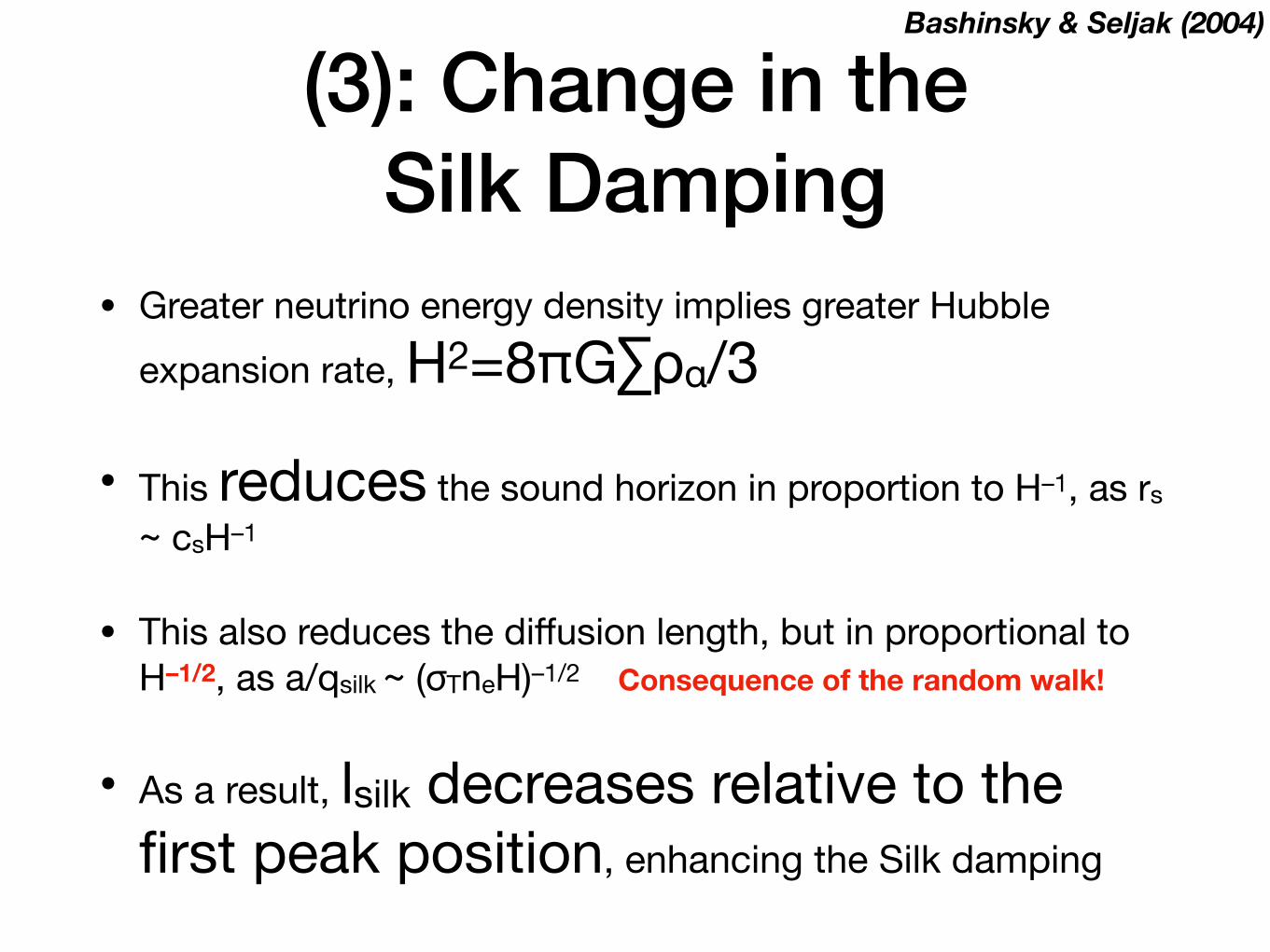
(3): Change in the Silk Damping

• Greater neutrino energy density implies greater Hubble expansion rate, Η2=8πG∑ρα/3

• This reduces the sound horizon in proportion to H–1, as rs ~ csH–1

• This also reduces the diffusion length, but in proportional to H–1/2, as a/qsilk ~ (σTneH)–1/2

• As a result, lsilk decreases relative to the first peak position, enhancing the Silk damping

Consequence of the random walk!

Bashinsky & Seljak (2004)

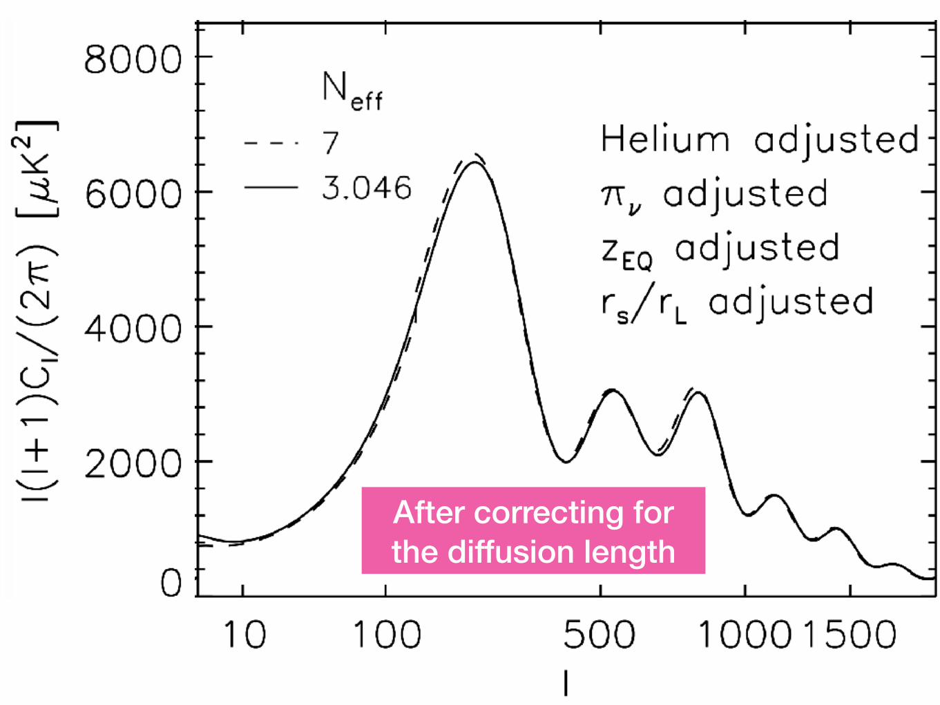
After correcting for the diffusion length

Zoom in!

(4): Viscosity Effect on the Phase of Sound Waves

The solution is

where

Hu & Sugiyama (1996)

Bashinsky & Seljak (2004)

Phase shift!

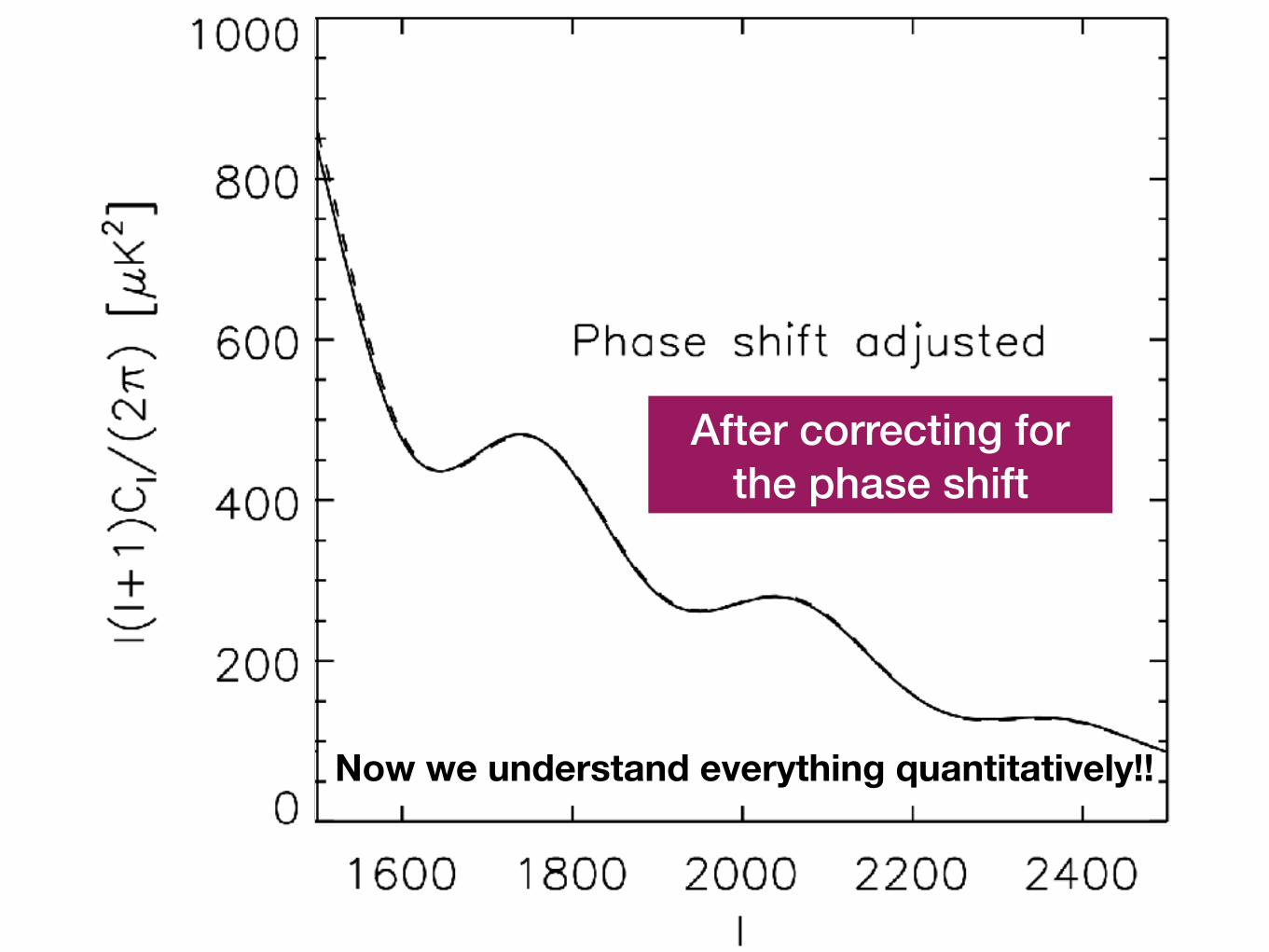
After correcting for the phase shift

Now we understand everything quantitatively!!

Two Other Effects• Spatial curvature

• We have been assuming spatially-flat Universe with zero curvature (i.e., Euclidean space). What if it is curved?

•Optical depth to Thomson scattering in a low-redshift Universe

• We have been assuming that the Universe is transparent to photons since the last scattering at z=1090. What if there is an extra scattering in a low-redshift Universe?

Spatial Curvature• It changes the angular diameter distance, dA,

to the last scattering surface; namely,

• rL -> dA = R sin(rL/R) = rL(1–rL2/6R2) + … for positively-curved space

• rL -> dA = R sinh(rL/R) = rL(1+rL2/6R2) + … for negatively-curved space

Smaller angles (larger multipoles) for a negatively curved Universe

late-time ISW

Optical Depth

• Extra scattering by electrons in a low-redshift Universe damps temperature anisotropy

•Cl -> Cl exp(–2τ) at l >~ 10

• where τ is the optical depth

re-ionisation

• Since the power spectrum is uniformly suppressed by exp(–2τ) at l>~10, we cannot determine the amplitude of the power spectrum of the gravitational potential, Pφ(q), independently of τ.

• Namely, what we constrain is the combination: exp(–2τ)Pφ(q)

Important consequence of the optical depth

• Breaking this degeneracy requires an independent determination of the optical depth. This requires POLARISATION of the CMB.

/ exp(�2⌧)As

+CMB LensingPlanck

[100 Myr]

Cosmological Parameters Derived from the Power Spectrum

CMB Polarisation

• CMB is weakly polarised!

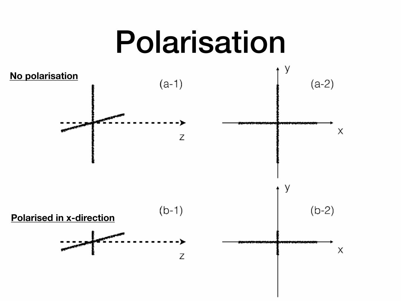
PolarisationNo polarisation

Polarised in x-direction

Photo Credit: TALEX

horizontally polarised

Photo Credit: TALEX

Photo Credit: TALEX

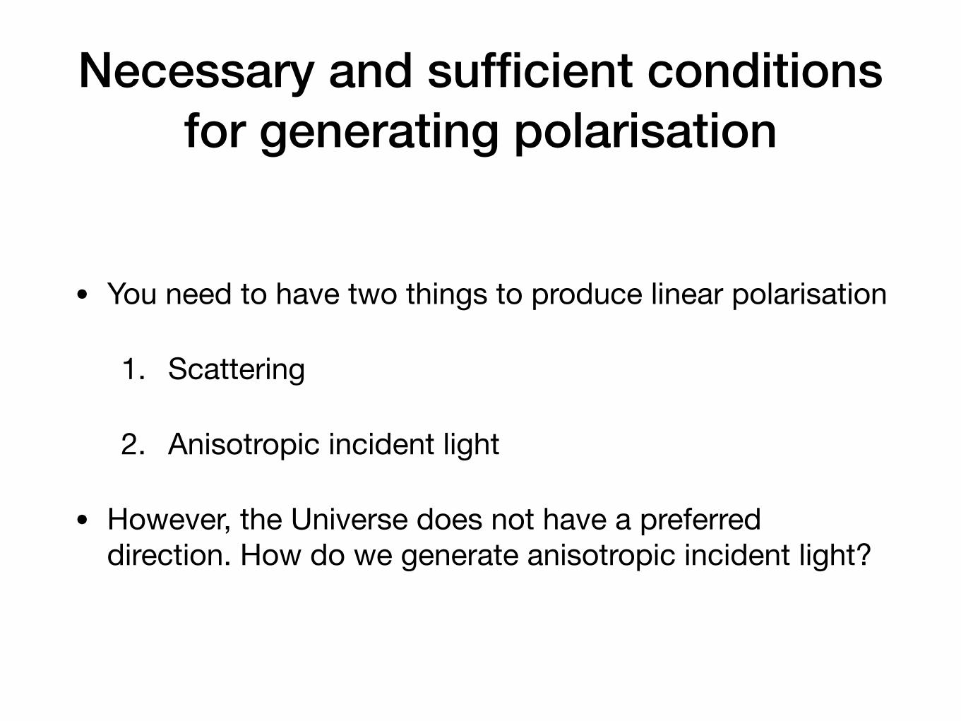
Necessary and sufficient conditions for generating polarisation

• You need to have two things to produce linear polarisation

1. Scattering

2. Anisotropic incident light

• However, the Universe does not have a preferred direction. How do we generate anisotropic incident light?

Wayne Hu

Need for a local quadrupole temperature anisotropy

• How do we create a local temperature quadrupole?

(l,m)=(2,0) (l,m)=(2,1)

(l,m)=(2,2)

Quadrupole temperature anisotropy seen from an electron

Quadrupole Generation: A Punch Line

• When Thomson scattering is efficient (i.e., tight coupling between photons and baryons via electrons), the distribution of photons from the rest frame of baryons is isotropic

• Only when tight coupling relaxes, a local quadrupole temperature anisotropy in the rest frame of a photon-baryon fluid can be generated

• In fact, “a local temperature anisotropy in the rest frame of a photon-baryon fluid” is equal to viscosity

Stokes Parameters [Flat Sky, Cartesian coordinates]

ab

Stokes Parameters change under coordinate rotation

x’y’Under (x,y) -> (x’,y’):

Compact Expression

• Using an imaginary number, write

Then, under coordinate rotation we have

Alternative Expression

• With the polarisation amplitude, P, and angle, , defined by

Then, under coordinate rotation we have

We write

and P is invariant under rotation

E and B decomposition• That Q and U depend on coordinates is not very

convenient…

• Someone said, “I measured Q!” but then someone else may say, “No, it’s U!”. They flight to death, only to realise that their coordinates are 45 degrees rotated from one another…

• The best way to avoid this unfortunate fight is to define a coordinate-independent quantity for the distribution of polarisation patterns in the sky

To achieve this, we need to go to Fourier space

n̂ = (sin ✓ cos�, sin ✓ sin�, cos ✓)

“Flat sky”, if θ is small

Fourier-transforming Stokes Parameters?

• As Q+iU changes under rotation, the Fourier coefficients change as well

• So…

where

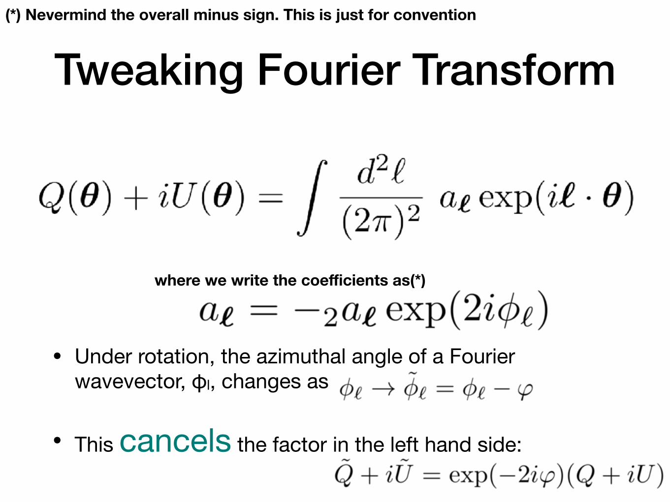
Tweaking Fourier Transform

• Under rotation, the azimuthal angle of a Fourier wavevector, φl, changes as

• This cancels the factor in the left hand side:

where we write the coefficients as(*)

(*) Nevermind the overall minus sign. This is just for convention

Tweaking Fourier Transform• We thus write

• And, defining

By construction El and Bl do not pick up a factor of exp(2iφ) under coordinate rotation. That’s great! What kind of polarisation patterns do

these quantities represent?

Seljak (1997); Zaldarriaga & Seljak (1997); Kamionkowski, Kosowky, Stebbins (1997)

Pure E, B Modes• Q and U produced by E and B modes are given by

• Let’s consider Q and U that are produced by a single Fourier mode

• Taking the x-axis to be the direction of a wavevector, we obtain

Pure E, B Modes• Q and U produced by E and B modes are given by

• Let’s consider Q and U that are produced by a single Fourier mode

• Taking the x-axis to be the direction of a wavevector, we obtain

Geometric Meaning (1)

•E mode: Polarisation directions parallel or perpendicular to the wavevector

•B mode: Polarisation directions 45 degree tilted with respect to the wavevector

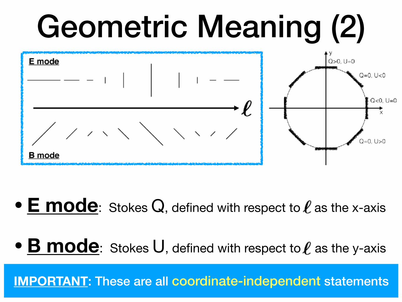
Geometric Meaning (2)

•E mode: Stokes Q, defined with respect to as the x-axis

•B mode: Stokes U, defined with respect to as the y-axis

IMPORTANT: These are all coordinate-independent statements

Parity

•E mode: Parity even

•B mode: Parity odd

Parity

•E mode: Parity even

•B mode: Parity odd

Power Spectra

• However, <EB> and <TB> vanish for parity-preserving fluctuations because <EB> and <TB> change sign under parity flip

B-mode from lensing

Antony Lewis

E-mode from sound waves

Temperature from sound waves

B-mode from GW

We understand this