Microsoft® Office Excel 2010: Level 1

Table of Contents

Lesson 1: Getting Started with Excel

A: Identify the Elements of the Excel Interface .......................................................................................... 7

B: Navigate and Select Cells in Worksheets ............................................................................................ 15

C: Customize the Excel Interface ............................................................................................................. 19

D: Create a Basic Worksheet .................................................................................................................. 24

6

Lesson 1

Getting Started with Excel

Lesson Objectives

In this lesson, you will create a basic worksheet by using Microsoft Excel 2010.

You will:

Identify the elements of the Excel interface.

Navigate and select cells in worksheets.

Customize the Excel interface.

Create a basic worksheet.

Introduction

You often work with data, but may not be aware that Microsoft Excel 2010 enables users to store and manage data better. Knowing that using Excel 2010 has several advantages, you are ready to learn the details. In this lesson, you will familiarize yourself with the Excel 2010 environment, customize the interface, and create a basic worksheet.

Using an instrument without the basic knowledge of its components and operating procedures can be a complicated task. Similarly, it would be difficult to use a software application such as Excel without understanding its interface elements and tools. Excel 2010 provides an interactive interface with enhanced features that help you create professional workbooks to store and analyze data easily.

7

Topic A

Identify the Elements of the Excel Interface

You are interested in the efficiency that can be realized by using the Excel application for storing and manipulating data. Before you gain this efficiency, you need to be familiar with its interface. In this topic, you will identify the elements of the Excel interface.

Wouldn't it be easy to work at a new job if you were fully acquainted with the tasks involved? Similarly, exploring Excel's interface will help you familiarize yourself with the options available in the application, which in turn, will help you use the application effectively.

Before using the Excel application, you need to be familiar with its interface. In this topic, you will identify the elements of the user interface.

Microsoft Excel 2010

Excel is an application in the Microsoft Office suite that you can use to create, revise, and save data in a spreadsheet format. You can also add formulas and functions to perform calculations, and analyze, share, and manage information using charts and tables. Excel also has options for adding pictures, shapes, and screenshots to a spreadsheet.

The Excel Application window

When you launch Excel, two windows are displayed, one within the other. The outer window is the main application window that usually fills the entire screen, and provides various interactive tools and commands. The inner window is the workbook window where you will work with data.

Figure 1-1: The components of an Excel application window.

Component Description

The Quick Access toolbar A toolbar that provides you with an easy access to frequently used application commands.

The Ribbon A panel that displays relevant commands to a particular set of tasks. These commands are organized into different tabs and groups.

The Formula Bar

A bar that displays the contents of the selected cell in a spreadsheet and can be used to type a formula or function. It also displays a reference to the active cell or the range of the current selection of cells.

The task pane A pane that appears on an as-needed basis and provides you with several options for a particular command selected on the Ribbon. You can move and resize the task pane.

The status bar A window element that is displayed at the bottom, and contains features such as dynamic zoom slider and a customizable status display.

8

The Ribbon

The Ribbon is an interface component that comprises several task-specific commands, which are grouped together under various tabs. It is designed to be the central location for accessing commands in the Microsoft Office suite for performing both simple and advanced operations without having to navigate extensively.

Figure 1-2: The Ribbon displaying the commands of the Home tab.

Ribbon Tab Used To

File Display the Backstage view that contains commands to print, save, and share workbooks.

Home Format spreadsheet data, add basic data and cell formatting, and add styles.

Insert Insert text, tables, charts, symbols, illustrations, and links.

Page Layout Specify page settings, layout, orientation, margins, and other options related to printing a workbook.

Formulas Create formulas with built-in functions to calculate values automatically. The built-in functions are categorized by the type of calculations they can perform.

Data Connect with external data sources and import data for use within Excel worksheets.

Review Review Excel worksheets. It also provides tools such as spell checker, thesaurus, and translator.

View Control the display of the worksheet and the workbook window. You can also hide or display the gridlines in a worksheet.

ScreenTips

A ScreenTip is descriptive text that is displayed when you position the mouse pointer over a component in the interface.

An enhanced ScreenTip describes the component in detail and often provides a link to a help topic. Most of the components in Excel have associated enhanced ScreenTips. Excel provides you with options to select the level of detail you want ScreenTips to display. Additionally, there are options in the Excel Options dialog box to turn off the ScreenTips.

The Backstage View

The Backstage view is an interface element with options that group similar commands. This view is designed to simplify access to Excel features and can be used to save, send, print, open workbooks, display document information, and customize the application. You can access the Backstage view from the File tab.

Figure 1-3: The Backstage view in Excel.

9

Option Description

Save, Save As, Open, and Close Allows you to save the changes made to a workbook, save a workbook with a new file name in the desired location, open an existing workbook, and close a workbook.

Info Displays options to protect workbooks by using a password, check for accessibility and compatibility issues, manage versions of workbooks, and set workbook properties.

Recent Lists workbooks that were recently accessed. It also allows you to customize the recently opened workbooks list by adding, removing, or reordering the items in the list.

New

Displays options to create a blank workbook, or a workbook based on a predefined or custom designed templates, or an existing workbook. You can also access additional templates from the Office.com website.

Print Displays options to preview and print workbooks.

Save & Send Provides options to save a workbook in a previous version of Excel, share a workbook through email or SharePoint, and publish a workbook.

Help Allows you to access the online and offline help resources. It also provides access to the Excel Options dialog box.

Options Displays the Excel Options dialog box, which allows you to customize the Excel interface.

Exit Allows you to exit the application.

The Quick Access Toolbar

The Quick Access toolbar is usually located above the Ribbon and is displayed as an integrated component of the title bar. It provides easy access to commonly used commands such as Save, Undo, and Redo. The Customize Quick Access Toolbar menu options not only allow you to customize the display of buttons, but also reposition the Quick Access toolbar below the Ribbon. You can also add frequently used commands either from the Ribbon or by selecting options from the Excel Options dialog box.

Figure 1-4: The default commands on the Quick Access toolbar.

The Status Bar

The status bar, located at the bottom of the Excel application window, displays the current mode and cell information, such as average, count, and sum. It also has elements for adjusting the zoom level of the displayed worksheet and for selecting the desired page layout option.

Element Function

The Mode indicator Displays current mode of Excel along with the information of any special key, which is engaged.

The Auto Calculate indicator Displays the average and sum of current selection along with the count of selected cells.

View buttons Provides options to display a worksheet in any of the three default views: Normal, Page Layout, and Page Break Preview.

The Zoom Out button Allows you to view the content in a worksheet in a smaller size.

The Zoom slider Allows you to magnify or diminish a worksheet view to any

desired size.

The Zoom In button Allows you to enlarge the view of worksheet contents.

The Zoom level button Allows you to set the zoom percentage of a worksheet.

10

The View Buttons on the Status Bar

The view buttons on the status bar enable you to view a worksheet in different views.

View Button Allows You To

Normal View a worksheet in the normal view.

Page Layout View a worksheet as it will appear on a printed page.

Page Break Preview

View a preview of a worksheet where the pages will break when the worksheet is printed.

The Formula Bar

The Formula Bar, located below the Ribbon, contains the Name Box, the Insert Function button, and the Formula Bar text box. The Name Box displays the name or reference of the selected cells. The Insert Function button enables you to insert a function in the selected cell. The Formula Bar text box displays the contents of the selected cell and allows you to edit the contents. You can expand, collapse, resize, or hide the Formula Bar to suit your preferences.

Figure 1-5: The Formula Bar on a worksheet.

Contextual Tabs

Contextual tabs are additional tabs that appear on the Ribbon when you select a specific object such as a chart, table, drawing, or text box. Because these tabs are context based, the commands displayed on the Ribbon depend upon the object that you select. These contextual tabs keep the number of tabs displayed on the Ribbon to a minimum and disappear once the relevant object is deselected.

Figure 1-6: A contextual tab displayed on the Ribbon.

11

Templates

Definition

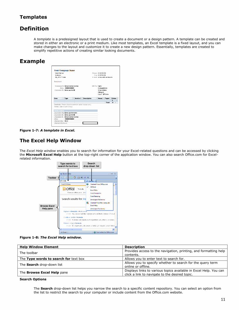
A template is a predesigned layout that is used to create a document or a design pattern. A template can be created and

stored in either an electronic or a print medium. Like most templates, an Excel template is a fixed layout, and you can make changes to the layout and customize it to create a new design pattern. Essentially, templates are created to simplify repetitive actions of creating similar looking documents.

Example

Figure 1-7: A template in Excel.

The Excel Help Window

The Excel Help window enables you to search for information for your Excel-related questions and can be accessed by clicking the Microsoft Excel Help button at the top-right corner of the application window. You can also search Office.com for Excel-

related information.

Figure 1-8: The Excel Help window.

Help Window Element Description

The toolbar Provides access to the navigation, printing, and formatting help contents.

The Type words to search for text box Allows you to enter text to search for.

The Search drop-down list Allows you to specify whether to search for the query term online or offline.

The Browse Excel Help pane Displays links to various topics available in Excel Help. You can click a link to navigate to the desired topic.

Search Options

The Search drop-down list helps you narrow the search to a specific content repository. You can select an option from

the list to restrict the search to your computer or include content from the Office.com website.

12

How to Identify the Elements of the User Interface

Procedure Reference Open a Workbook Using the Open Dialog Box

To open a workbook using the Open dialog box:

1. Select the File tab and choose Open to display the Open dialog box. 2. Navigate to the desired file and click Open.

New Workbooks

You can select the New option on the File tab to open a new workbook. When you select New, the Backstage view

displays the available templates organized in various categories from which to choose. You can choose to create a blank workbook, a workbook based on a template, or an existing workbook.

Activity 1-1

Identifying the Elements of the User Interface

Data Files

Sales Revenue.xlsx

Scenario

You have joined Our Global Company (OGC) Stores as a sales manager. In your job role, you need to use Excel application to analyze information. You have not worked with the Excel application previously; you want to familiarize yourself with the interface elements of the Excel application.

What You Do How You Do It

1. Explore the Backstage view and open a workbook.

a. Choose Start→All Programs→Microsoft Office→Microsoft Excel 2010to launch the Microsoft

Excel 2010 application.

b. If necessary, in the User Name dialog box, click OK.

c. In the Welcome to Microsoft Office 2010 dialog box, select the Don`t make changes option and click OK.

d. On the Ribbon, select the File tab to display the Backstage view.

e. Observe that the File menu consists of options to save, open, print, and close a workbook. From the menu,

choose New.

f. Under the Available Templates section, view the available templates and then from the File menu, choose Open to display the Open dialog box.

g. Navigate to the C:\084576Data\Getting Started with Excel folder.

h. Select the Sales Revenue.xlsxfile and click Open.

13

2. Explore the Ribbon tabs.

a. On the Ribbon, select the Page Layout tab to view its commands.

b. Observe that the Themes, Page Setup, Scale to Fit, Sheet Options, and Arrange groups are displayed along with the relevant commands.

c. In the Page Setup group, place the mouse pointer over any button to view its ScreenTip.

d. Select the other tabs on the Ribbon to view the commands and groups on them.

3. Explore the Quick Access toolbar.

a. On the Quick Access toolbar, place the mouse pointer over each button to view its description.

b. At the right end of the Quick Access toolbar, click the Customize Quick Access Toolbar drop-down arrow to display the Customize Quick Access Toolbar menu.

c. View the options available on the Customize Quick Access Toolbar menu and click the Customize Quick Access Toolbar drop-down arrow to close the menu.

14

4. Explore the status bar.

a. On the status bar, to the left of the Zoom slider, place the mouse pointer over each of the buttons to view their descriptions.

b. At the right end of the status bar, click the Page Layout button, which is the second button from the left, to change the layout of the worksheet.

c. Click the Page Break Preview button which is located to the right of Page Layout button.

d. In the Welcome to Page Break Preview message box, click Onto view the worksheet with page breaks.

e. At the right end of the status bar, on the Zoom slider, click the Zoom In button.

f. Observe that the zoom percentage has increased to 70%.

g. Click the Zoom Out button and observe that the zoom percentage has reverted to 60%.

h. Click the Normal button which is located to the left of Page Layout button to return to the normal view.

15

Topic B

Navigate and Select Cells in Worksheets

You familiarized yourself with the interface components of the Excel application. To view or modify data in Excel, you need to know how to work with worksheets. In this topic, you will navigate through an Excel worksheet.

Imagine that you have just moved to a new city to start a new job. To reach your office, you want to try the various modes of transport available in the city and decide on the quickest and the easiest option. Learning the basics of navigating in Excel is very similar to this; you know how to commute, but you need to familiarize yourself with the commuting options available. By navigating through Excel, you will familiarize yourself with the interface, thus making it easier for you to work with Excel.

To view or modify data in Excel, you need to know how to work with worksheets. In this topic, you will navigate through an Excel worksheet.

Spreadsheets

Definition A spreadsheet is a paper or an electronic document that is used to store and manipulate data. It consists of rows and columns that intersect to form cells, where the data you enter is stored. Data can be in the form of numbers, text, and non-alphanumeric symbols in a tabular format. You can customize spreadsheets based on your business needs and data requirements.

Example

Figure 1-9: A spreadsheet with data.

Worksheets

A worksheet is an electronic spreadsheet that is used for entering and storing data in Excel. An Excel worksheet contains columns and rows, which intersect like a grid to form cells. Excel designates columns with alphabetical headers running across the top of the worksheet, and rows with numerical headers running down the left of the worksheet. An Excel worksheet can contain various types of data such as text, numbers, pictures, formulas, charts, or tables. You can insert or delete rows, columns, and cells from an Excel worksheet.

Figure 1-10: An Excel worksheet.

16

Worksheet Referencing Elements

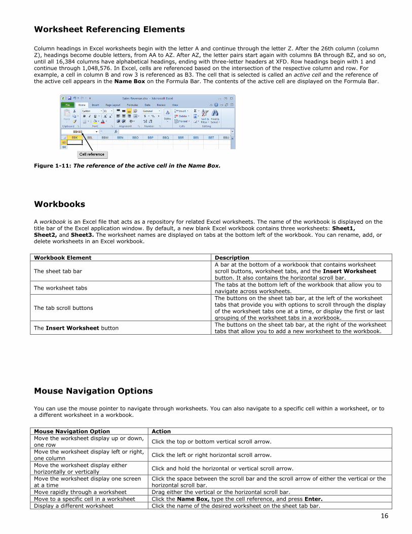
Column headings in Excel worksheets begin with the letter A and continue through the letter Z. After the 26th column (column Z), headings become double letters, from AA to AZ. After AZ, the letter pairs start again with columns BA through BZ, and so on, until all 16,384 columns have alphabetical headings, ending with three-letter headers at XFD. Row headings begin with 1 and continue through 1,048,576. In Excel, cells are referenced based on the intersection of the respective column and row. For example, a cell in column B and row 3 is referenced as B3. The cell that is selected is called an active cell and the reference of the active cell appears in the Name Box on the Formula Bar. The contents of the active cell are displayed on the Formula Bar.

Figure 1-11: The reference of the active cell in the Name Box.

Workbooks

A workbook is an Excel file that acts as a repository for related Excel worksheets. The name of the workbook is displayed on the title bar of the Excel application window. By default, a new blank Excel workbook contains three worksheets: Sheet1, Sheet2, and Sheet3. The worksheet names are displayed on tabs at the bottom left of the workbook. You can rename, add, or delete worksheets in an Excel workbook.

Workbook Element Description

The sheet tab bar A bar at the bottom of a workbook that contains worksheet scroll buttons, worksheet tabs, and the Insert Worksheet

button. It also contains the horizontal scroll bar.

The worksheet tabs The tabs at the bottom left of the workbook that allow you to navigate across worksheets.

The tab scroll buttons

The buttons on the sheet tab bar, at the left of the worksheet tabs that provide you with options to scroll through the display of the worksheet tabs one at a time, or display the first or last grouping of the worksheet tabs in a workbook.

The Insert Worksheet button The buttons on the sheet tab bar, at the right of the worksheet tabs that allow you to add a new worksheet to the workbook.

Mouse Navigation Options

You can use the mouse pointer to navigate through worksheets. You can also navigate to a specific cell within a worksheet, or to a different worksheet in a workbook.

Mouse Navigation Option Action

Move the worksheet display up or down, one row

Click the top or bottom vertical scroll arrow.

Move the worksheet display left or right, one column

Click the left or right horizontal scroll arrow.

Move the worksheet display either horizontally or vertically

Click and hold the horizontal or vertical scroll arrow.

Move the worksheet display one screen at a time

Click the space between the scroll bar and the scroll arrow of either the vertical or the horizontal scroll bar.

Move rapidly through a worksheet Drag either the vertical or the horizontal scroll bar.

Move to a specific cell in a worksheet Click the Name Box, type the cell reference, and press Enter.

Display a different worksheet Click the name of the desired worksheet on the sheet tab bar.

17

Keyboard Navigation Options

You can use a keyboard to navigate within and across worksheets in a workbook to enter, view, or modify data.

Keyboard Navigation Option Action

Move one cell to the left, right, up, or down

Press the Up, Down, Left, or Right arrow key.

Move to column A of the current row

Press Home.

Scroll down or up by one screen Press Page Down or Page Up.

Scroll one screen to the left or right Press Alt+Page Down or Alt+Page Up.

Move to the cell on the right Press Tab.

Move to the cell on the left Press Shift+Tab.

Move to cell A1 Press Ctrl+Home.

Navigate across worksheets Press Ctrl+Page Up or Ctrl+Page Down.

Move to the last column of the current row

Press End.

Move to the first or last column or row of data

Press Ctrl along with the Up, Down, Left, or Right arrow key.

Cell Selection Options

Excel provides you with multiple options to select a cell or a group of cells in a worksheet. You can select either a contiguous range consisting of cells that are adjacent to each other, or a noncontiguous range consisting of cells that are not adjacent to each other.

Selection Option Action

A cell Click the cell.

A contiguous range Select the first cell in the range, hold down Shift, and select the last cell of the range. Alternatively, you can click and drag from the first cell of the range to the last cell of the range.

A noncontiguous range

Select the first cell in the first range, hold down Ctrl, and click the next cell in the range. To select multiple cells, hold down Ctrl and click multiple cells. You can also select multiple contiguous range of cells that are noncontiguous by using the Shift+click and Ctrl+click methods.

An entire row or column Click the alphabetical header of a column or the numerical header of a row.

An entire worksheet Click the Select All button below the Name Box.

How to Navigate and Select Cells in Worksheets

Procedure Reference Navigate and Select Cells in a Worksheet

To navigate and select cells in a worksheet:

1. Open a workbook. 2. Use the appropriate navigation techniques to move to the desired location.

Click in the Name Box, type the cell reference, and presenter to move to a specific cell in the worksheet.

Click the vertical or bottom scroll bar to move the worksheet display up or down.

Press the Up, Down, Left, or Right arrow key to move one cell up, down, left, or right, respectively.

3. Use the appropriate selection methods to select cells.

Click the cell to select the cell.

Select the first cell in the range, hold down Shift, and select the last cell of the range.

Click and drag from the first cell of the range to the last cell of the range to select a continuous range of cells.

18

Activity 1-3

Working with Cells in Excel

Setup

Before You Begin:

The Sales Revenue.xlsx file is open.

Scenario

You want to familiarize yourself with the sales trend for your team to prepare a report on your team's performance for the past year. The sales information is stored in an Excel workbook. You need to view the relevant information of each sales person from this workbook.

What You Do How You Do It

1. View specific cells in the worksheet.

a. Scroll down to view the data in row 83.

b. Hold down Ctrl and press Home to navigate to the beginning of the worksheet. Hold down Ctrl and press Home.

c. Hold down Ctrl and press Page Down to move to the next worksheet. Hold down Ctrl and press Page Down.

d. Observe that Sheet2 is selected.

e. On the sheet tab bar, clickSheet1 to return to the first worksheet.

2. Select a continuous range of cells.

a. Scroll down and select cell A83.

b. Hold down Shift and click cellM84 to select a range of cells from A83 to M84. Hold down Shift and click cell M84.

c. At the top-left corner of the worksheet, below the Name Box, click the Select All button to select the entire worksheet.

3. Select a non-continuous range of cells.

a. Scroll up and select cell A19.

b. Hold down Shift and click cellE19. Press Shift and click cellE19.

c. Observe that the cells A19 to E19 are selected.

d. Hold down Ctrl and click cell H19.

e. Hold down Shift and click cellJ19. Hold down Shift and click cell J19.

f. Observe that a non-continuous range of cells is selected.

g. Click on any empty cell to deselect the selection.

19

Topic C

Customize the Excel Interface

You navigated through and selected content in an Excel worksheet. There may be instances when the default display and arrangement of the interface elements does not suit your preference. Excel provides you with options to personalize the interface according to your requirements. In this topic, you will customize the Excel interface.

When you start working with a new software application, the interface may not provide you with convenient access to all the options that you require, or the interface may be cluttered with options that you may not require at all. A cluttered interface can compromise your work efficiency. By customizing the application's interface, you will be able to access the options that you need easily and quickly.

There may be instances when the default display and arrangement of the interface elements does not suit your preference. Excel provides you with options to personalize the interface according to your requirements. In this topic, you will customize the Excel interface.

The Excel Options Dialog Box

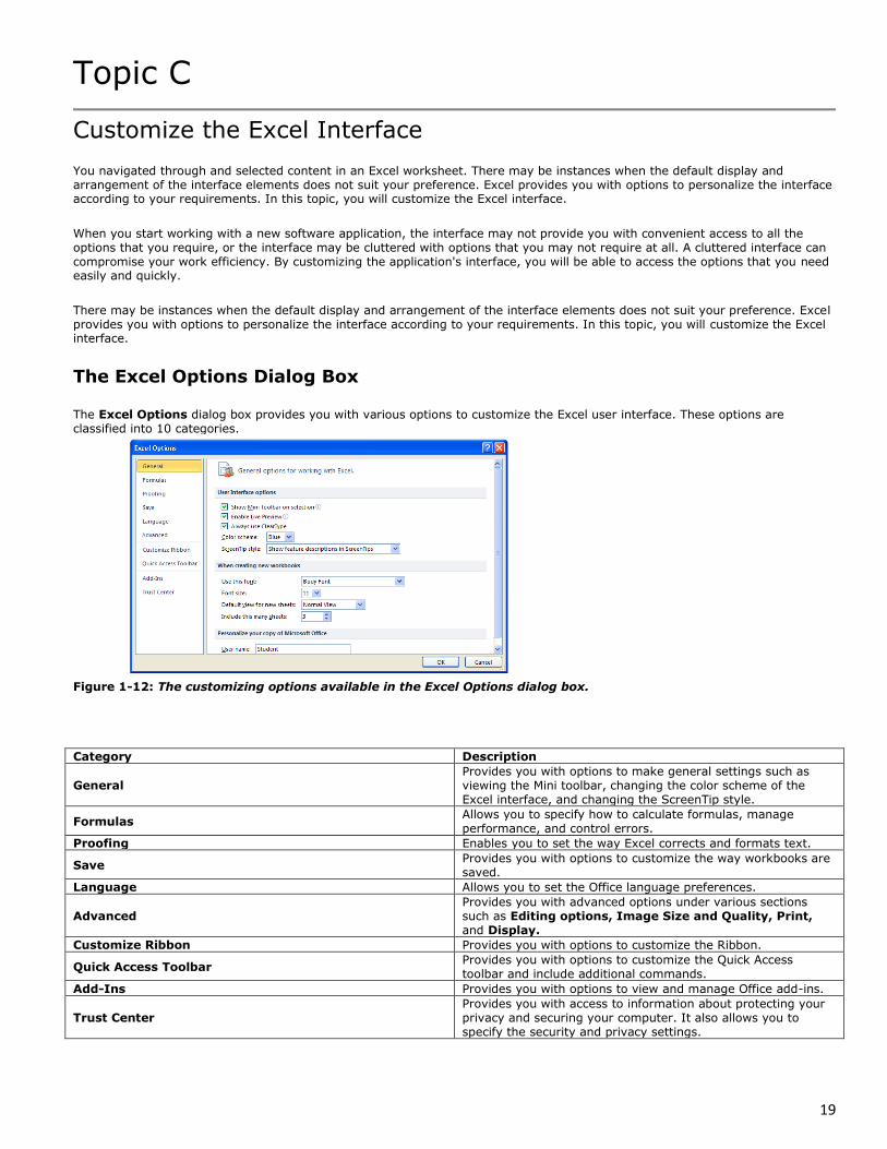
The Excel Options dialog box provides you with various options to customize the Excel user interface. These options are classified into 10 categories.

Figure 1-12: The customizing options available in the Excel Options dialog box.

Category Description

General Provides you with options to make general settings such as viewing the Mini toolbar, changing the color scheme of the Excel interface, and changing the ScreenTip style.

Formulas Allows you to specify how to calculate formulas, manage performance, and control errors.

Proofing Enables you to set the way Excel corrects and formats text.

Save Provides you with options to customize the way workbooks are saved.

Language Allows you to set the Office language preferences.

Advanced Provides you with advanced options under various sections such as Editing options, Image Size and Quality, Print, and Display.

Customize Ribbon Provides you with options to customize the Ribbon.

Quick Access Toolbar Provides you with options to customize the Quick Access toolbar and include additional commands.

Add-Ins Provides you with options to view and manage Office add-ins.

Trust Center Provides you with access to information about protecting your privacy and securing your computer. It also allows you to specify the security and privacy settings.

20

How to Customize the Excel Interface

Procedure Reference Customize the Quick Access Toolbar Using the Excel Options Dialog Box

To customize the Quick Access toolbar using the Excel Options dialog box:

1. Display the Quick Access Toolbar tab of the Excel Options dialog box.

Select the File tab and choose Options, and in the Excel Options dialog box, click Quick Access Toolbar or;

From the Customize Quick Access Toolbar menu, choose More Commands. 2. From the Choose commands from drop-down list, select the category from which you want to add a command.

3. In the Choose commands from list box, select the desired command and click Add to add the command to the Quick Access toolbar.

4. If necessary, click the Move Up or Move Down arrow button located on the right of Customize Quick Access Toolbar list box to move the options up or down the list.

You can also reposition the Quick Access toolbar below the Ribbon by selecting the Show Below the Ribbon option from the Customize Quick Access Toolbar menu.

5. Click OK to close the Excel Options dialog box.

Procedure Reference Customize the ScreenTip Style

To customize the ScreenTip style:

1. Select the File tab and choose Options. 2. If necessary, in the Excel Options dialog box, select the General tab. 3. Under the User Interface options section, from the ScreenTip style drop-down list, select an option.

Select Show feature descriptions in ScreenTips to display the name of the element along with a brief

description.

Select Don't show feature descriptions in ScreenTips to display only the name of the element.

Select Don't show ScreenTips to disable ScreenTips. 4. Click OK to apply the new ScreenTip style.

Procedure Reference Add a Command Button from the Ribbon to the Quick Access Toolbar

To add a command button or group from the Ribbon to the Quick Access toolbar:

1. On the Ribbon, select the tab that has the desired command button or group. 2. Add the desired command button or group.

Right-click the command button and choose Add to Quick Access Toolbar.

Within the desired group, right-click the text region below the buttons and choose Add to Quick Access Toolbar.

Procedure Reference Customize the Status Bar

To customize the status bar:

1. At the bottom of the application window, right-click the status bar to display the Customize Status Bar menu. 2. From the displayed menu, choose the required options.

On the menu, when you choose an option, a check mark is displayed to its left to indicate that the selected option is displayed on the status bar. Selecting an option that has a check mark will hide the information on the status bar.

3. Click away from the Customize Status Bar menu to close it.

21

Procedure Reference Customize the Save Options

To customize the save options:

1. Select the File tab and choose Options. 2. In the Excel Options dialog box, select the Save tab. 3. In the Save workbooks section, set the save options.

From the Save files in this format drop-down list, select a format.

In the Save Auto Recover information every text box, type the number of minutes to specify the duration

after which Auto Recover information is saved.

In the Default file location text box, type the path of the default location in which workbooks are saved. 4. Click OK to apply the customized options.

Procedure Reference Customize the Ribbon

To customize the Ribbon:

1. Select the File tab and choose Options. 2. In the Excel Options dialog box, select the Customize Ribbon tab. 3. In the Customize the Ribbon list box, check or uncheck the check boxes for the tabs to show or hide the respective

tab on the Ribbon. 4. Create a new tab and group.

a. Below the Customize the Ribbon list box, click New Tab to create a tab. b. If necessary, below the Customize the Ribbon list box, click New Group to create a group.

5. Rename a tab or a group. a. In the Customize the Ribbon list box, select the tab or group that you want to rename. b. Display the Rename dialog box.

Below the Customize the Ribbon list box, click Rename or;

Right-click the tab or group and choose Rename.

c. In the Rename dialog box, type a new name and click OK. 6. Add commands to a group.

a. From the Choose commands from drop-down list, select the desired category from which you want to choose commands.

b. In the Choose commands from list box, select the desired command that you want to add. c. In the Customize the Ribbon list box, select the tab and group to which you want to add the command. d. Click Add to add the selected command.

7. If necessary, in the Customize the Ribbon list box, select a command and click Remove to remove the command from the group.

8. If necessary, create more tabs and groups and add commands to them. 9. Click OK to close the Excel Options dialog box.

22

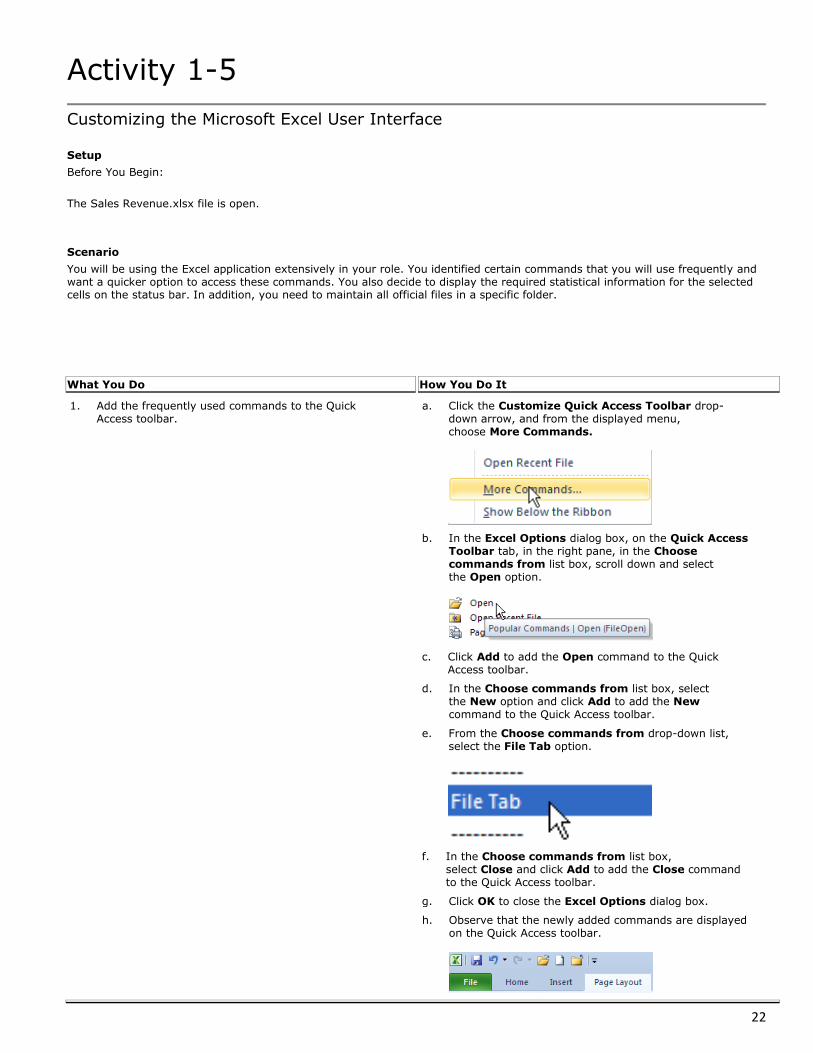
Activity 1-5

Customizing the Microsoft Excel User Interface

Setup

Before You Begin:

The Sales Revenue.xlsx file is open.

Scenario

You will be using the Excel application extensively in your role. You identified certain commands that you will use frequently and want a quicker option to access these commands. You also decide to display the required statistical information for the selected cells on the status bar. In addition, you need to maintain all official files in a specific folder.

What You Do How You Do It

1. Add the frequently used commands to the Quick Access toolbar.

a. Click the Customize Quick Access Toolbar drop-down arrow, and from the displayed menu, choose More Commands.

b. In the Excel Options dialog box, on the Quick Access Toolbar tab, in the right pane, in the Choose commands from list box, scroll down and select the Open option.

c. Click Add to add the Open command to the Quick Access toolbar.

d. In the Choose commands from list box, select the New option and click Add to add the New command to the Quick Access toolbar.

e. From the Choose commands from drop-down list, select the File Tab option.

f. In the Choose commands from list box, select Close and click Add to add the Close command to the Quick Access toolbar.

g. Click OK to close the Excel Options dialog box.

h. Observe that the newly added commands are displayed on the Quick Access toolbar.

23

2. Add the Alignment group to the Quick Access toolbar.

a. On the Ribbon, select the Home tab.

b. In the Alignment group, right-click on the text “Alignment” and choose Add to Quick Access Toolbar.

c. On the Quick Access toolbar, click the Alignment button to display the options in the Alignment group.

d. Observe that all the Alignment group options are now accessible from the Quick Access toolbar and then click the Alignment button to close the Alignment group.

3. Customize the status bar.

a. On the status bar, right-click to view the Customize Status Bar menu.

b. From the displayed menu, choose Macro Recording.

c. Observe that a check mark is displayed beside the Macro Recording option denoting that Macro Recording is added to the status bar and the macro recording icon is displayed in the status area of the status bar.

d. Choose Maximum and Minimum to add them to the status bar.

e. From the displayed menu, choose Zoom.

f. Observe that the check mark is removed and the zoom percentage that was displayed on the status bar is

hidden.

g. Click away from the menu to close the Customize Status Bar menu.

4. Set the default location and color scheme.

a. Select the File tab and choose Options.

b. In the Excel Options dialog box, verify that the General tab is selected.

c. In the User Interface Options section, from the Color scheme drop-down list, select Blue.

d. In the Excel Options dialog box, select the Save tab.

e. In the Save workbooks section, in the Default file location text box, triple-click and type the excel folder name that you created on your desktop and click OK.

f. Observe that the blue theme is applied.

g. On the Quick Access toolbar, choose Close to close the file.

24

Topic D

Create a Basic Worksheet

You customized the Excel interface to enable easy access to frequently used commands in Excel. To start using the Excel application, you need to add data to a worksheet and save it. In this topic, you will enter data in an Excel worksheet.

Bricks are put together to construct a building, and complex structures are achieved by combining the bricks in different forms. Similarly, basic data are put together to create complex worksheets. Before you begin to create complex worksheets, you should know how to enter basic data.

To start using the Excel application, you need to add data to a worksheet and save it. In this topic, you will create a basic worksheet.

Data Types

Excel allows you to enter various types of data. These data types can be generally categorized as labels, values, and dates and time. Labels are text that can be represented using letters, numbers, and symbols. Values are numbers that you may use to perform mathematical or statistical analysis. Date and time are used to represent date, time, or both in various formats. Depending on the data you enter in a cell, Excel automatically chooses the appropriate data type.

Excel 2010 File Formats

The default file type in Excel 2010 is (.xlsx) an XML-based file format. Files saved in this format are suffixed with the letter x. Using this XML-based file format allows files to be automatically compressed upon saving and decompressed upon opening. Saving spreadsheets in the default Excel 2010 file format not only allows you to secure data, but also recover data if the file is corrupt. Excel provides you with an extensive list of formats to save spreadsheets that can be shared with other users.

File Type Description

Excel Workbook (.xlsx)

The default file type in Excel 2010.

Excel Macro-Enabled Workbook (.xlsm)

A basic XML file type that can store VBA macrocode.

Excel 97–2003 Workbook (.xls)

The file type that is used to save a file in a format that is compatible with the previous versions of Excel.

Excel Template (.xltx)

The default file type for an Excel template. It is used to save a workbook as a template so that new workbooks can be created using its content, layout, and format.

Excel Macro-Enabled Template (.xltm)

The default file type for an Excel macro-enabled template.

Excel Binary Workbook (.xlsb)

The binary file format in Excel 2010.

Excel 97–2003 Template (.xlt)

The file type that enables you to save an Excel template that is compatible with the previous versions of Excel.

PDF (.pdf) The file type that enables you to save an Excel document as an Adobe Portable Document Format (PDF) file.

25

The Save and Save As Commands

The Save command is used to save a new workbook or the changes made to an existing workbook, without altering its name, file type, or location. The Save As command is used to save an existing file with a new name, file type, or location. These commands can be accessed from the File tab.

If you use the Save command when a workbook was not previously saved, the Save As dialog box will be displayed automatically.

The Save As Dialog Box

The Save As dialog box can be used to select a different folder, in which to save the file. The default name of the file is displayed in the File name text box. You can also specify a different file name for the file. From the Save as type drop-down list, you can select a different format in which to save the file.

The Compatibility Checker Feature

The Compatibility Checker feature in Excel 2010 allows you to identify the compatibility of objects and data in an Excel 2010 workbook, when you intend to save it in an earlier version of Excel. In the Microsoft Excel - Compatibility Checker dialog box, you can view a list of features in your Excel 2010 file that are not supported in earlier versions of Excel. The dialog box also provides you with an option to convert these objects so that they are visible in earlier versions of Excel. However, you will not be able to modify the objects once you convert them.

Figure 1-13: The Microsoft Excel Compatibility Checker dialog box.

26

How to Create a Basic Worksheet

Procedure Reference Create a Workbook and Enter Data

To create a workbook and enter data:

1. Select the File tab and choose New. 2. In the Backstage view, in the Available Templates pane, below the Home button, select Blank workbook. 3. In the right pane, in the Blank workbook pane, click Create. 4. In the new worksheet, enter the desired data. 5. Use the appropriate navigation technique to select the next cell where you want to enter data. 6. From the File tab menu, choose Save.

Procedure Reference Perform a Compatibility Check on a Workbook

To perform a compatibility check on a workbook:

1. Select the File tab and choose Info. 2. In the Backstage view, in the Prepare for Sharing section, from the Check for Issues drop-down list, select Check

Compatibility.

3. In the Microsoft Excel – Compatibility Checker dialog box, observe the features that are not supported in the earlier version of Excel and click Cancel.

Procedure Reference Save a Workbook Using the Save As Option

To save a workbook using the Save As option:

1. Select the File tab and choose Save As to display the Save As dialog box. 2. In the Save As dialog box, navigate to the desired folder. 3. In the File name text box, type a name for the file. 4. From the Save as type drop-down list, select the desired file format and click Save.

If you select a format of an earlier version of Excel, the Compatibility Checker feature will automatically check the file for any compatibility issues.

5. If necessary, in the Microsoft Excel - Compatibility Checker dialog box, click Continue to convert the features that are not supported in the earlier version of Excel.

Procedure Reference Recover Unsaved Workbooks

To recover unsaved workbooks:

1. On the File tab, select Recent. 2. In the Backstage view, in the right pane, select the Recover Unsaved Workbooks option. 3. In the Open dialog box, select the unsaved workbook and click Open.

27

Activity 1-7

Entering Data in an Excel Workbook

Scenario

OGC Stores has recently introduced two new products. You have the sales data for these products on a printed paper. You want to create an invoice with this data in an Excel worksheet to send it to a customer. You also need to send a copy of this invoice to a coworker in the accounting department who is using Excel 2003.

What You Do How You Do It

1. Enter the column headings.

a. On the Quick Access toolbar, click New to open a blank workbook.

b. In cell A1, type Product and press Tab to move to cell B1.

Type the text as indicated and press Tab.

c. In cell B1, type Quantity and press Tab. Type the text as indicated and press Tab.

d. In cell C1, type Price and press Tab. Type the text as indicated and press Tab.

e. In cell D1, type Date of Shipment and press Enter. Type the text as indicated and presenter.

2. Enter the name of the products.

a. Click cell A3, type Pen and presenter. Type the text as indicated and press Enter.

b. In cell A4, type Chart Type the text as indicated.

3. Enter the data for quantity.

a. Click cell B3, type 410 and presenter. Type the number as indicated and press Enter.

b. In cell B4, type 385 Type the number as indicated.

4. Enter the price and date of shipment.

a. Click cell C3, type 0.5 and presenter. Type the value as indicated and press Enter.

b. In cell C4, type 2 Type the value as indicated.

c. Enter today's date in cells D3 and D4.

5. Save the workbook in different file formats.

a. Select the File tab and choose Save.

b. Navigate to the Excel folder you created on your desktop.

c. In the Save As dialog box, in the File name text box, triple-click and type My Invoice and click Save.

d. Select the File tab and choose Save As.

e. In the Save As dialog box, from the Save as type drop-down list, select Excel 97–2003 Workbook (*.xls) and click Save to save the file in the XLS format.

f. On the Quick Access toolbar, click Close to close the file.

28

Lesson Labs

Due to classroom setup constraints, some labs cannot be keyed in sequence immediately following their associated lesson. Your instructor will tell you whether your labs can be practiced immediately following the lesson or whether they require separate setup from the main lesson content.

Lesson 1 Lab

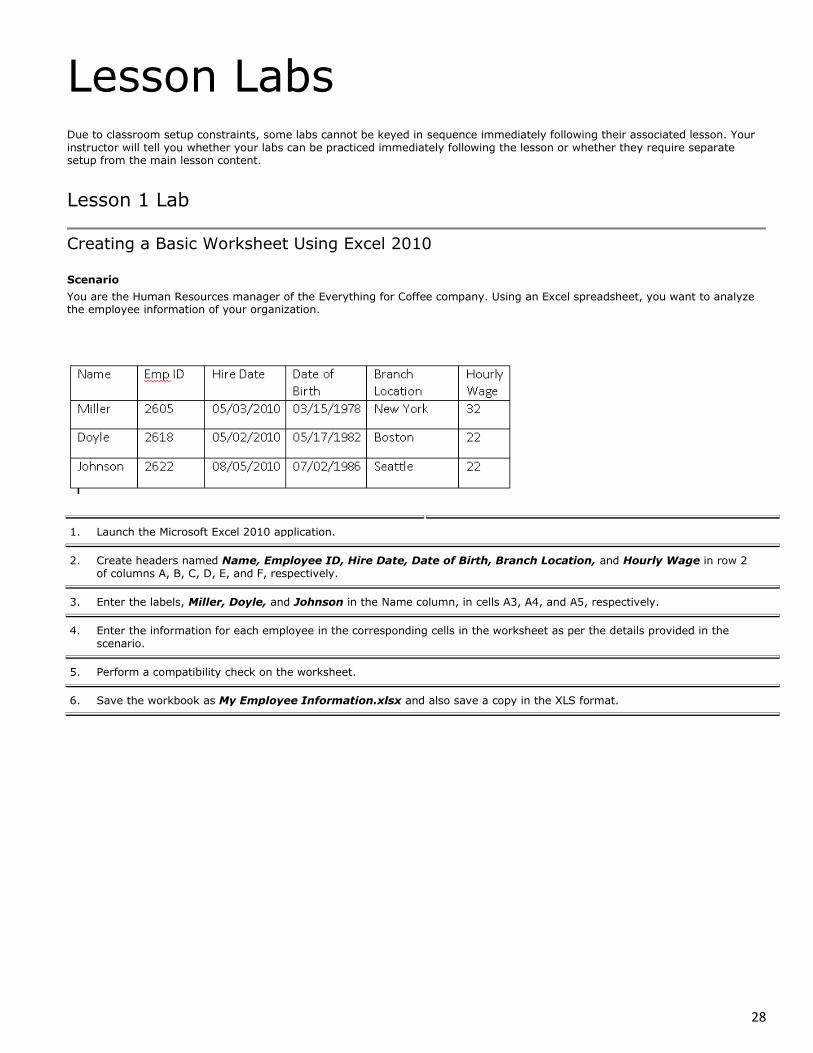
Creating a Basic Worksheet Using Excel 2010

Scenario

You are the Human Resources manager of the Everything for Coffee company. Using an Excel spreadsheet, you want to analyze the employee information of your organization.

1. Launch the Microsoft Excel 2010 application.

2. Create headers named Name, Employee ID, Hire Date, Date of Birth, Branch Location, and Hourly Wage in row 2 of columns A, B, C, D, E, and F, respectively.

3. Enter the labels, Miller, Doyle, and Johnson in the Name column, in cells A3, A4, and A5, respectively.

4. Enter the information for each employee in the corresponding cells in the worksheet as per the details provided in the scenario.

5. Perform a compatibility check on the worksheet.

6. Save the workbook as My Employee Information.xlsx and also save a copy in the XLS format.