1

Life Energy Meter Experimental Reports

http://www.heliognosis.com/rd.html Page

Measuring the Life Energy Phenomena in an Impatience Plant Leaf 1 Observations of vacuum fluctuations suggests the existence of Zero Point Energy (ZPE) 2 Visualizing Chakras Using the Experimental Life Energy Meter 6 Mapping the Energy Body 7 Measuring the Life Energy Phenomena in a Yeast Culture 15 The Response of Orgonotic Instruments to Atmospheric Conditions 16

Experimental Report 1:

Measuring the Life Energy Phenomena in an Impatience Plant Leaf

by David Marett B.Sc.

Impatience Flower

Background

In The Cancer Biopathy, Volume II of the Discovery of the Orgone (1948), Wilhelm Reich wrote at length about an energy concentration device that he called an Orgone Accumulator. Reich claimed this heretofore unknown energy caused a local rise in temperature within the accumulator. He further mentioned a second method of measuring this energy using a high voltage oscillating electric field connected unipolarly to a series of metal plates. A light bulb connected to these plates luminated when living things approached or were placed on the

test plate. Reich observed that a fresh fish placed on the test plate yielded a high lumination of the bulb. The longer the fish remained on the plate (after death) the weaker the lumination was. After several years of experimentation, Heliognosis has developed this method of life energy measurement into a compact electronic instrument. The following experiment illustrates the life energy measurement of a fresh leaf from the Impatience flower and shows how it diminishes with time after picking.

Test leaf inside zip-lock bag

Method

The Experimental Life Energy Meter Model LMII was placed on a plywood table with the small plate electrode directly behind it. A leaf from the Impatience plant was cut from the stem and placed into a weighed tight fitting

zip-lock bag. The air was fully removed from the bag before weighing. The initial weight of the leaf was 0.3 grams. The bag with the leaf inside was taped to the small plate electrode so that it was centered. The leaf could then be placed directly over the plate and then removed to one side for zeroing the meter by lifting one side of the masking tape. Measurements of the energy of the leaf were made once a day with zeroing before and after to confirm the

accuracy of the reading. All measurements were made on the x10 range and all other objects were kept at least 16 inches away from the meter.

Leaf moved away from plate for zeroing - Leaf on the plate for measuring

2

Observations

The leaf was intensely green and vibrant when it was picked. It remained flat during the experiment but the green colour faded slightly over nine days to a dark olive colour. As well, the taut appearance of the leaf tissue became flaccid and slightly wrinkled. The leaf's dimensions remained the same at 4" long and 1 1/8" wide and its weight remained constant. The readings of the energy diminished each day as indicated in the following graph.

Conclusion

The leaf's dimensions and weight remained constant, consistent with the prevention of water and mass loss by using the sealed zip-lock bag. The decrease in the energy readings could then only be caused by a loss of vitality as the leaf cells died after removal from the plant. This is initial evidence that leaves and perhaps all living or once living things contain an energy which dissipates with a loss of life or loss of vitality.

Experimental Report 2:

Observations of vacuum fluctuations suggests the existence of Zero Point Energy (ZPE)

by David Marett B.Sc.

Abstract

Recent experimental evidence would suggest that the elusive zero point energy (ZPE) vacuum fluctuations can be detected using an electric field. Initial data indicates that increasing electric field strength results in an increased coupling with the vacuum fluctuat-ions. This has been determined by varying both the voltage of the electric field as well as by increasing the surface area of the radiator plate. With an AC electric field of 246V peak-to-peak, the vacuum fluctuations present themselves as a dynamic quasi-cyclic current oscillation in the very low frequency (VLF) and ultra-low frequency (ULF) range with a magnitude of 0.02%.

Although Zero Point Energy Vacuum Fluctuations have become a well studied Quantum Mechanical concept, little experimental evidence has come forward in respect to the electric field. A recent study by R. Blanco, H. M. França, E. Santos and R. C. Sponchiado¹ in Physics Letters A, suggests that vacuum fluctuations for the magnetic field can be detected. These magnetic voltage fluctuations are shown to be experimentally distinguishable from the voltage fluctuations associated with the well known Nyquist noise¹.

While studying the electric field absorption in living subjects at a distance, a fluctuation was observed in the very low frequency (VLF) range. The observat-ions were made using a metal plate charged with AC

high voltage. Current flow to and from the plate was monitored using a high impedance, high gain electric current amplifier. Improvements in amplifier design reduced the "thermal Johnson noise" to a level two orders of magnitude lower than the peak-to-peak intensity of the fluctuations initially observed. An apparatus was assembled to study these fluctuations as shown in figure 1.

3

Setup

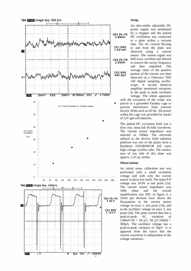
An ultra-stable adjustable DC power supply was modulated by a chopper and the pulsed DC oscillation was connected to a plate within a vacuum tube. The AC current flowing to and from the plate was observed using a current sensor. The current signal was half-wave rectified and filtered to remove the carrier frequency and then amplified. The average value of the positive portion of the current was then observed on a Tektronix TDS 320 digital sampling oscillo-scope. A second identical amplifier monitored variations in the peak to peak oscillator voltage. The whole apparatus

with the exception of the scope was placed in a grounded Faraday cage to prevent interference from external electric fields such as 60 Hz. All power within the cage was provided by stacks of 12V gel-cell batteries.

The pulsed DC excitation field was a slow rise, steep fall 66 kHz waveform. The current sensor impedance was selected as 100kΩ. The electrode utilized as the electric field radiation platform was one of the plates from a Raytheon JAN5R4WGB full wave high voltage rectifier tube. The surface area of one side of this plate was approx. 2.25 sq. inches.

Observations

An initial noise calibration test was performed with a small excitation voltage and with only the current sensor in place (no load). The input P-P voltage was 16.8V at test point (2a). The current sensor impedance was 100k ohms and the overall amplification was 50X. In figure 3, a 25mS per division trace shows the fluctuations in the current sensor voltage on trace 1, test point (1b), and in the oscillator voltage on trace 2, test point (2b). The plate current then has a peak-to-peak AC variation of 2.88mV/50 = 58 µV, 58 µV/100kΩ = 580pA. The oscillator voltage has a peak-to-peak variation of 58µV. It is apparent from the traces that the current waveform is independent of the voltage variations.

4

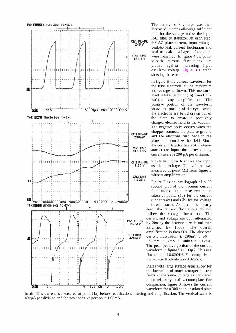
The battery bank voltage was then increased in steps allowing sufficient time for the voltage across the input R-C filter to stabilize. At each step, the AC plate current, input voltage, peak-to-peak current fluctuation and peak-to-peak voltage fluctuation were measured. In figure 4 the peak-to-peak current fluctuations are plotted against increasing input oscillator voltage. Fig. 4 is a graph showing these results.

In figure 5 the current waveform for the tube electrode at the maximum test voltage is shown. This measure-ment is taken at point (1a) from fig. 2 without any amplification. The positive portion of the waveform shows the portion of the cycle when the electrons are being drawn out of the plate to create a positively charged electric field in the vacuum. The negative spike occurs when the chopper connects the plate to ground and the electrons rush back to the plate and neutralize the field. Since the current detector has a 20x attenu-ator at the input, the corresponding current scale is 200 µA per division.

Similarly figure 6 shows the input oscillator voltage. The voltage was measured at point (2a) from figure 2 without amplification.

Figure 7 is an oscillograph of a 50 second plot of the vacuum current fluctuations. This measurement is taken at points (1b) for the current (upper trace) and (2b) for the voltage (lower trace). As it can be clearly

seen, the current fluctuations do not follow the voltage fluctuations. The current and voltage are both attenuated by 20x by the detector circuit and then amplified by 1000x. The overall amplification is then 50x. The observed current fluctuation is 296mV / 50 = 5.92mV. 5.92mV / 100kΩ = 59.2nA. The peak positive portion of the current waveform in figure 5 is 290µA. This is a fluctuation of 0.0204%. For comparison, the voltage fluctuation is 0.0256%.

Plates with large surface areas allow for the formation of much stronger electric fields at the same voltage as compared to the relatively small vacuum plate. For comparison, figure 8 shows the current waveform for a 300 sq in. insulated plate

in air. This current is measured at point (1a) before rectification, filtering and amplification. The vertical scale is 400µA per division and the peak positive portion is 1.03mA.

5

Similarly the voltage waveform and ultra-low frequency (ULF) fluctuations are shown in figures 9 and 10 respectively. In figure 10, the current fluctuations (upper trace) have a scale of 40nA per division. The peak-to-peak current fluctuation was 81.6nA or 0.0079%. The voltage fluctuation was 0.0081%.

Demonstration of the vacuum fluctuation using the Heliognosis Model LM2

A commercial version of the above circuit, the Heliognosis Experimental Life Energy Meter LM2, was connected in the Faraday cage and operated from a 12V gel cell battery. The meter was allowed to warm up for 30 minutes before measurements were taken to insure stability. To rule out the effects of temperature, all the readings were taken over a period of 30 minutes and the temperature was monitored with a mercury thermometer. The temperature at the beginning of the experiment was 17.4 C. At the end of the experiment, the temperature was 17.1 C. The LM2 has a much stronger damping filter than the laboratory version used above to allow observation of the fluctuations outside

of a Faraday cage. The stronger filtration reduces the observed fluctuations some-what but also filters 60Hz more effecti-vely. A smaller flat plate was first tested (40sq in) with the amplification set to x1000 and the rear switch in the large plate position (200kΩ sensor impedance). A large plate, model LM03-AC, with a surface area of 300 sq in was next conn-ected with the same operating conditions. The zero controls were adjusted for each plate to keep the average reading on the analog meter around 10%. The chart recorder output was connected to the TDS320 DSO and provided oscillographs of the VLF and ULF fluctuations.

6

Observations

Readings were taken with the oscilloscope in AC mode to observe the VLF fluctuations in the low Hertz range. These readings were taken over periods of 250mS and 1 second. The oscilloscope was switched to DC mode to see both VLF and ULF fluctuations together over a period of 100 seconds. Several readings in both modes were taken with the small and large plates and the averaged data is shown below.

Peak-to-peak fluctuations:

Figure 11 shows an example of the large plate AC fluctuations over a period of 0.25 sec. As can be seen, the VLF current fluctuation is quasi-cyclic with several frequencies such as 11.5Hz, 25Hz and 40Hz. Electromagnetic interference such as 60Hz is effectively blocked by the Faraday cage and is not visible in the waveform.

Figure 12 shows an example of the DC fluctuations for the large plate over a 100 second interval. The combined VLF and ULF fluctuation corresponds to a peak to peak value of 21.4 nA.

Conclusions

From the above results it is apparent that the electric field around a vacuum plate fluctuates dynamically with a quasi-cyclic oscillation in the VLF and ULF range. The AC current to the vacuum plate varies by as much as 0.0204% within the input voltage and current range studied. The vacuum fluctuations were found to increase proportionately to the input plate voltage. It was also found that increasing plate area also increases the fluctuations. The effective conclusion is that the electric permittivity is not constant but rather a function of the local zero point energy vacuum fluctuations.

References

¹ R. Blanco, H. M. França, E. Santos and R. C. Sponchiado. Radiative noise in circuits with inductance. Physics Letters A, Volume 282, Issue 6, 30 April 2001, Pages 349-356

Experimental Report 3:

Visualizing Chakras Using the Experimental Life Energy Meter

by David Marett B.Sc.

The following procedure demonstrates how to obtain an energetic signature from a human subject using the Heliognosis LM2 Experimental Life Energy Meter. Figure 1 illustrates the mechanical scanning method. An LM2 meter was supported by a nylon cable from a pulley mounted on the ceiling of the laboratory. A geared motor drove the pulley such that the meter would lower itself to the floor at a constant speed. A second nylon

AC (VLF only) DC (VLF+ULF)

small plate 7.9nA 11.2nA

large plate 12.3nA 21.4nA

7

guide cable was employed to keep the meter moving straight as it descended and prevent horizontal motion. The recorder output from the LM2 was connected to a chart recorder so that a plot of the energy signature would be obtained. Every scan used the vacuum tube electrode. This report focuses on a series of scans performed on myself using this method. The results provide a 2-D rendering of my energy field as would be seen by an observer viewing from the side.

The scans were performed at average distances between 3" and 12" from the vacuum tube sensor to obtain energy field depth information. A total of seven scans were performed, four from the front and three from the back. The meter moved from ceiling to floor at a constant rate of 0.88 ft/sec.

1. The Root Chakra (Muladora): In this region the energy field compresses close to the body. A small peak is detectable from the rear on the three inch scan at this chakra.

2. Navel chakra (Swadisthana): The energy begins to expand at this point.

3. Solar Plexus chakra (Manipara): The energy field expands to a peak, projecting predominantly forward.

4. Heart chakra (Anahata): The energy from the Anahata or Heart Chakra is held very close to the back while projecting intensely from the subject's chest. The overall field at this point is attenuated compared to the Manipara chakra.

5. Throat chakra (Vishudha): The energy field projects strongly to the rear.

6. Third eye chakra (Agna): Measuring upward the energy continues to decrease although there is a distinct emanation from the front of the body.

7. Crown chakra (Sahasraram): The field decreases to a minimum here.

In the leg area the energy field emanates from the back of the body with a peak at the knee. As the scanner approaches the ground, increased readings are caused by energy from the earth.

Furthest from the body we find that the solar plexus projection is the most intense at the front. From the rear the throat chakra projects furthest.

Experimental Report 4: http://www.heliognosis.com/rd04.html#exp04

Mapping the Energy Body

by David Marett B.Sc.

The idea that an energy body surrounds the human form has endured since ancient times. The Tibetan Book of the Dead1 refers to it in a ritualistic speech made to the dying to prepare them for the states they are about to encounter. Carlos Castaneda discusses it at great length in his famous apprenticeship to become a warrior and to sidestep the destruction of his awareness at the moment of death2. Wilhelm Reich described an energy he called Orgone, which pervaded everything and was concentrated in living organisms3. Despite having been described by many cultures and researchers an objective method to observe the energy body has remained elusive.

Energy Body Theories

The Chakra system of interpretation identifies the primary energy concentrations in the body. These are defined as the crown of the head, the third eye at the center of the forehead, the throat, the heart (comprised of a center, left and right side), the solar plexus, the navel and the genitalia or root 4. This system originated in Asia and is not perceived

8

directly by the practitioner. In contrast, Carlos Castaneda claimed that he was taught to actually see the energy body by following the practices carried down from the Toltecs. Castaneda depicted the energy body as being shaped like an oblong egg encased in a cocoon that stretches seven feet above the ground and four feet wide5. According to his descriptions, the energy body could potentially escape through the crown during moments of intense stress. The head was considered to be the center of reason and talking. The tip of the sternum was the center of feeling. The center below the naval was the will, and the genital and anal region were final energy concentrations in the lower body. In addition, the left side of the ribs was considered the center for seeing and the right side the center for dreaming6. Castaneda mentions a total of eight energy centers as opposed the nine within the Chakra system. As well, Castaneda stresses that the energy center of the body is also the geometric center of the body. Another feature of the energy body unique to Castaneda is the presence of an assemblage point where awareness is manifest, located on the back over the right shoulder blade7.

To contrast Reichian energetic theory, the proper flow of energy is from the core to the periphery and back to the core cyclically. The pulsation of the body Orgone is associated with deep breathing and oxygenation of the tissues as well as orgastic charge and discharge. The primary energy centers for a Reichian energy perspective is the solar

plexus and the heart/lungs for breathing and the genitals for orgastic potency8. These three regions together form the core with the center around the solar plexus area.

Instrumentation

Techniques such as Kirlian photography have been used to visualize the portion of the energy body which emanates from the fingertips or hands. This technique has been used to evaluate the overall health of the person by analyzing the strength and quality of the electric field patterns around the fingers. Although Kirlian photography will remain a valuable technique, it remains limited to indirect measurement of the quality and shape of the energy body.

The Orgone Field Meter of Wilhelm Reich employed a similar sensing field to the Kirlian method. Using an optically coupled galvanometer, Reich was able to sense the decline of vitality in plants and fish as a function of time after death. His device however was limited to the observation of the overall energy and was not able to provide an energetic map for the body. The Orgone Field Meter principle and the Kirlian principle are both based on the ability of living tissue to differentially absorb and radiate electric displacement currents. This same principle has been improved upon and has been built into a scanning system that can detect the energy body up to a distance of 60 cm. By employing this scanning method, a profile of the energy body may be created from head to toe. A picture of the scanning apparatus is shown at the left.

The scanner is composed of a plastic tubular frame with a low speed motor drive. The motor allows the Experimental Life Energy Meter to descend or ascend at a fixed speed of 1ft/sec. The sensitivity of the meter is selected so that the subject will be 6 inches to 1 foot away from the tube sensor. The optimum range is x100 and the zero is set to zero when there is no subject present and the meter is midway through its travel. Switches at the top and bottom of the frame stop the meter travel as it arrives. Because these switches are connected inductively to ground, the meter reading increases quickly as it approaches them. In order to avoid such effects, all extraneous objects should be kept at least 18 inches away from the scanner during the procedure.

The subject stands facing the scanning frame and the operator activates the Life Meter to descend. The data is collected by a data acquisition system and plotted graphically on the computer display. The image is then saved into an image-processing program. The subject then stands facing away from the scanner while the operator scans the energy profile from behind. These two images are then composed with a picture of the subject on the computer to form the complete energy profile.

Typical Male and Female Scans

In figure 1a a 32 year old healthy male exhibits a typical energy pattern. To the left of the male figure is a graph of the data collected from the rear of the body. To the right is the plot of the energy from the front of the body. The graphs are coloured to show the regions of interest. Each graph has a scale for the energy intensity from zero to eight. These areas are coloured in the following way:

• Purple: Crown of the head and the region immediately above the head

• Sky blue: Eyes

• Dark blue: Throat and upper shoulders

• Green: Heart

• Yellow: Solar plexus

• Orange: Naval

• Red: Genitals or root

9

This subject is a healthy young adult male that will be used to compare the relative strengths and weaknesses of the energy pattern of other male subjects. This will be done by comparing the intensity of the energy at each level as well as its direction, forward or behind. The coloured bar graph in figure 1b shows the combined average of the front and rear readings at each of the above levels. Again the maximum reading is eight.

Referring now to figure 1a, we can see that the energy begins to expand starting 6 inches above the head. A local peak in the energy field is then observed at the level of the eyes. Around the throat, the energy field begins to expand gradually into the heart region. This peak is most noticeable at the rear of the body. The energy field then pushes forward to a peak at the front of the body at the solar plexus region while drawing in slightly at the rear. The energy field then reaches a second major peak at the rear of the body at the pelvis. At the front the energy field begins to close in on itself gradually below the solar plexus. The field then draws inward around the genitalia reaching a minimum around knee level. Below 1.5 feet from the ground, the influence of the earth causes a sudden increase in the energy reading. Looking at the average energy of each level we can see that the heart has the strongest emanation followed by the naval and solar plexus.

A healthy female, 29 years old, is shown in figure 2a. Looking at the energy body from the front, her field begins to expand 12 inches above the head. A noticeable peak can be observed at eye level. The throat region shows a gradual increase with a peak at the base of the neck as seen from the rear, roughly corresponding to the "assemblage point" described by Carlos Castaneda. The female field expands forward at the heart while the energy is drawn in slightly at the rear. Forward expansion continues peaking at the solar plexus while, at the rear, the energy peaks at the naval. The energy body then draws inward around the genitalia and reaches a minimum in the mid thigh. From the average energy data, we can see that the female has her highest energy level at the naval followed by the solar plexus and heart. All of the following female subjects will use her scan as a reference for comparison.

The male energy above the head has an average value of 1.8 compared to 2.4 for the female. The female energy above the head is also visible 6" higher than the male. The female energy is also greater at the eye level at 4.4 compared to the male at 3.2. The same trend continues at the throat with the female at 5.5 contrasted with the male average reading at 4.6. This trend begins to reverse at the heart where the average male reading peaks at 6.3 vs 5.9 for the female. The female again averages higher at the solar plexus at 6.4 vs 6 for the male. At the naval, the female

10

has the highest average at 6.7 vs 6.1 for the male. Around the genitalia, the female is 5.5 vs 4.5 for the male. Around the legs where the energy is lowest, the female is 4.8 and the male is 3.4.

From the above numerical analysis, it can be seen that the male energy is on average strongest at the heart. The energy is evenly distributed around the solar plexus and is located at the centre of gravity for the adult male. The male exhibits two major peaks at the heart and naval regions. Looking only at the front energy, the peaks are at the eyes and solar plexus. From the rear, the peaks are at the eyes, heart and naval.

For the female, the strongest average energy is at the naval level. The naval is the only average peak for the female. This also corresponds with the natural centre of gravity for an adult female. From the front, the female exhibits peaks at the eyes, heart and solar plexus. From the rear, the peaks are at the heart and naval.

From a Reichian perspective, the core of the organism would contain the greatest amount of Orgone energy. For the typical male, the energy is concentrated in the heart and lungs in contrast to the female, whose energy is strongest in the diaphragm and womb areas. The main forward energy peak of both male and female corresponds to the physical center of the body in agreement with Castaneda's assertion as well as the conception that we are connected to the world by an invisible thread of energy emanating from our solar plexus region. It is possible that the energy peak that everyone exhibits around the shoulder blade area may correspond to the "assemblage point". Men's enhanced heart area would indicate that they have a natural affinity for feeling, seeing and dreaming. The naval peak in the female energy body may be due to a concentration of energy in the womb. The aura around the body is affected by various lifestyle, health, vitality and psychological conditions and the scans may be used to help identify these conditions.

Subjects for Comparison

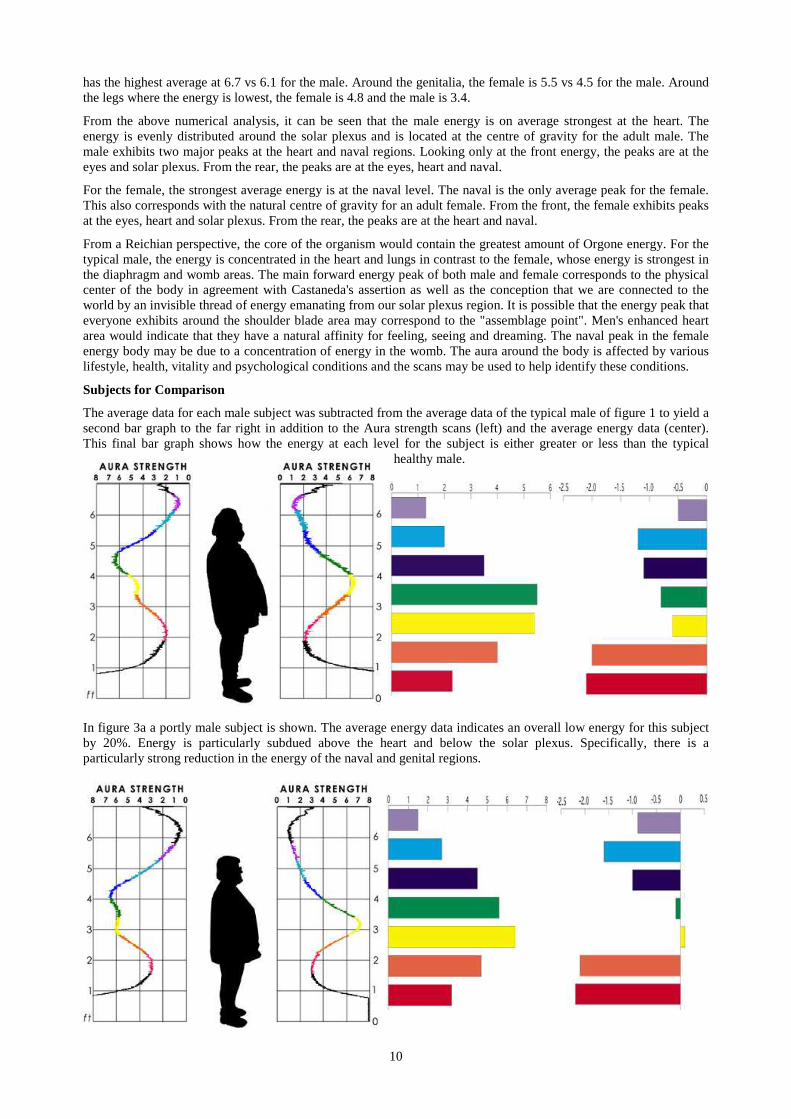
The average data for each male subject was subtracted from the average data of the typical male of figure 1 to yield a second bar graph to the far right in addition to the Aura strength scans (left) and the average energy data (center). This final bar graph shows how the energy at each level for the subject is either greater or less than the typical

healthy male.

In figure 3a a portly male subject is shown. The average energy data indicates an overall low energy for this subject by 20%. Energy is particularly subdued above the heart and below the solar plexus. Specifically, there is a particularly strong reduction in the energy of the naval and genital regions.

11

Figure 4a shows a portly female subject. Her average data is subtracted from the average data of the typical female in figure 2a and displayed in the bar graph figure 4b. As with the portly male, the average energy data indicates a generally reduced energy of about 15%. The naval and genital regions are close to normal but the throat and head regions are weak. From the front and rear energy chart, the forward energy can be seen to be concentrated exclusively at the solar plexus.

Figure 5a is a 37-year-old mother of two. Her overall health is good but she has a minor digestive and growth disorder. Comparing her to the typical female, her average energy pattern is virtually the same above the heart. Her heart energy though is stronger than normal by 10%. This is also evident from the heart peak from her frontal energy scan. She has a reduction in energy at the genital area of 15%. In this particular case, the overall energy is normal and strong. The elevation of energy from the lower part of the body towards the heart may be due to a highly relaxed state. Evidence for this will be illustrated in figure 13a.

Figure 6a shows a second, 45 yr old, mother of two who has suffered from a digestive ailment but is otherwise healthy. Her average energy pattern is almost identical to the previous woman and exhibits a slight reduction below the heart. Organ damage in the solar plexus and naval region may be responsible for the 15% reduction in energy in that region. It is interesting to note that the reduction in energy in the lower part of the body is almost exclusively at the rear.

Old age does not dramatically effect the aura if the health is good. As can be seen in the male of figure 7a, the energy around the heart is projected predominantly backward and the root energy is drawn towards the front of the body. Head and solar plexus energy remains normal. From the average data, it is clear that there has been a significant reduction in the heart energy with the maximal peak now for the solar plexus/naval regions. From the front energy profile, it is apparent that the overall energy of the body has shifted downward towards the naval. There is about a 10% reduction in overall energy.

12

In figure 8a is shown an elderly female subject. The average energy profile is very similar to the typical female except for a 20% reduction in the above head and eye energy levels. The front profile also confirms that the energy body has become more concentrated around the solar plexus and naval region. At the rear of the body, the energy at the solar plexus level is almost equal to that of the heart and naval areas.

In figure 9a is the energy profile of a spiritual healer. It is interesting to note that her frontal energy is concentrated in the solar plexus area exclusively. This in confirmed by both the average data as well as the front scan data. This would be in agreement with the shamanic will emanations from this region for healing.

13

Figure 10a shows a woman who is under great psychological stress. Her centres of reason (head) are over stimulated and emanating with a particularly strong projection. Her heart and throat energy have been borrowed for this task. Her solar plexus energy resembles that of a healer, being focused intensely. Her entire energy field is compressed overall by about 20%. It is likely that this energy compression is a form of spiritual defense.

In figure 11a is shown an 11-year-old boy. His weight and health are normal but his personality is dominated by sports and aggressive behavior. The aggressive child has a diffuse frontal energy shape almost uniformly projecting from head to root. Overall his energy is very strong, 10-15% higher than normal, especially from the head. It is interesting to note that children, with a smaller frame than adults, yield a more intense energy profile.

In figure 12a, another 11-year-old boy is shown who avoids physical activity and invests his energy predominantly on computer and video games. The virtual child has an enhanced eye energy with an intense projection of reason and intellectualization of almost 30%. There is a corresponding reduction in the heart, naval and genitals. The overall energy of his body is normal.

14

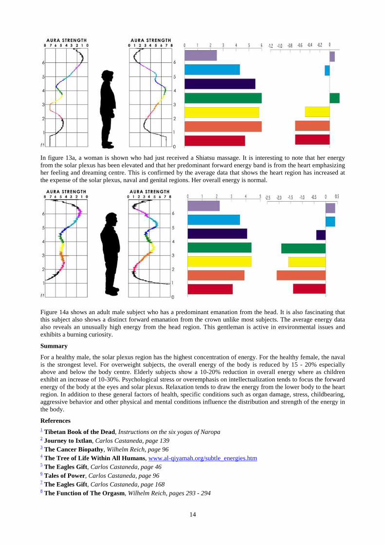
In figure 13a, a woman is shown who had just received a Shiatsu massage. It is interesting to note that her energy from the solar plexus has been elevated and that her predominant forward energy band is from the heart emphasizing her feeling and dreaming centre. This is confirmed by the average data that shows the heart region has increased at the expense of the solar plexus, naval and genital regions. Her overall energy is normal.

Figure 14a shows an adult male subject who has a predominant emanation from the head. It is also fascinating that this subject also shows a distinct forward emanation from the crown unlike most subjects. The average energy data also reveals an unusually high energy from the head region. This gentleman is active in environmental issues and exhibits a burning curiosity.

Summary

For a healthy male, the solar plexus region has the highest concentration of energy. For the healthy female, the naval is the strongest level. For overweight subjects, the overall energy of the body is reduced by 15 - 20% especially above and below the body centre. Elderly subjects show a 10-20% reduction in overall energy where as children exhibit an increase of 10-30%. Psychological stress or overemphasis on intellectualization tends to focus the forward energy of the body at the eyes and solar plexus. Relaxation tends to draw the energy from the lower body to the heart region. In addition to these general factors of health, specific conditions such as organ damage, stress, childbearing, aggressive behavior and other physical and mental conditions influence the distribution and strength of the energy in the body.

References 1 Tibetan Book of the Dead, Instructions on the six yogas of Naropa 2 Journey to Ixtlan, Carlos Castaneda, page 139 3 The Cancer Biopathy, Wilhelm Reich, page 96 4 The Tree of Life Within All Humans , www.al-qiyamah.org/subtle_energies.htm 5 The Eagles Gift, Carlos Castaneda, page 46 6 Tales of Power, Carlos Castaneda, page 96 7 The Eagles Gift, Carlos Castaneda, page 168 8 The Function of The Orgasm, Wilhelm Reich, pages 293 - 294

15

Experimental Report 5:

Measuring the Life Energy Phenomena in a Yeast Culture

by David Marett B.Sc.

Background

Until now the only way to determine if cells are alive or dead is by using subjective observations such as movement, the presence of metabolism products, consumption of media, production of gasses etc. The vigor and health of cells can only be indirectly measured. Wilhelm Reich illustrated in the Bion Experiments and later in The Cancer Bio-pathy that cell vigor could be monitored using special techniques such as dark-field microscopy. Using apochromatic objectives, the blue energetic glow of healthy cells could be seen directly at high magnification. Similarly, Reich treated human blood with a salt solution and observed the length of time before cell death using the dark-field technique. By careful observation of the cell contraction and eventual time of cell membrane breakage, he was able to determine the overall energetic strength of the blood cells and of the person from whom they were taken. In this report a method for monitoring cell culture growth and cell vitality is presented using the Heliognosis LM3 Experimental Life Energy Meter in conjunction with a liquid/cell culture probe.

Fluid Probe Apparatus and LM3

Reference solution and culture

Method:

The Heliognosis Experimental Life Energy Meter Model LM3 Rev B. was placed on a frame with the reference and sample liquid electrodes mounted behind. The apparatus was positioned on a wooden table with all other objects moved at least 18 in away. Two test tube solutions were prepared, each containing exactly 10ml of pure water1. The two tubes were screwed into the reference and sample electrodes. The calibration adjustment was carefully rotated until both the reference and sample electrode read exactly 0% on the x100 range of the Life Meter. To the sample tube was added 0.8 g of Lantic white granulated sugar. The meter now read 9%. The sample tube was then unscrewed and 0.2g of Baker's yeast (Fleischmann's) was added. The tube was immediately screwed into the sample electrode and the timer started.

Observations:

Immediately upon re-attaching the sample electrode with the yeast solution, the reading was 12%. The yeast initially sank to the bottom of the tube. A cloudiness gradually began to form and was distinct after 13 minutes. After 20 minutes, bubbling began from the bottom of the solution. The room temperature was 19.5 degrees C.

When the yeast culture had been growing for 33 minutes, it was observed that the culture was rising to the top of the solution and a gas filled foam developed. At this point the readings on the meter, that had been increasing gradually, began to climb more rapidly. The reference electrode was periodically checked using the switch on the liquid probe to make sure that the instrument was still calibrated. If the reference had deviated away from zero, the Life Meter zero was adjusted to keep the readings accurate. From 40 minutes onward the surface culture continued to grow finally to a thickness of 7mm between 94 and 135 minutes. Gasses and culture solution would occasionally overflow from the vent hole as the growth progressed. Excess was wiped away to prevent it from altering the reading of the inside culture growth. After 135 minutes, the evolution of gas and the rate of culture growth dropped rapidly with the collapse of the surface culture. The deposit of yeast at the bottom of the tube was now much smaller. Bubbling continued from below but at a much lower rate. The culture's activity became insignificant beyond 325 minutes with only occasional bubbles rising from the bottom. Below is shown a picture of the cell culture after 104 minutes. The Life Meter data is plotted graphically below and shows the detected energy level of the culture over time.

16

Yeast culture on solution surface - Detected energy level of yeast culture over time

Conclusion:

The visual observations of culture growth and decline matched perfectly with the data recorded from the Life Meter. During their life cycle, the cells accumulated energy and then released it again to the environment. It is now apparent that the displace-ment currents utilized by the Life Meter can detect the Life energy present in these cells and can monitor its increase and decrease over the cells life cycle. This may lead to the possibility of differential diagnosis of cell health.

Notes: 1Luso bottled water, contains 41.6 ppm of dissolved salts

The Response of Orgonotic Instruments to Atmospheric Conditions

Experimental Report 8; by Heliognosis http://www.heliognosis.com/rd.html#exp08

Abstract

Atmospheric Orgone energy and weather conditions are compared using the To-T apparatus, the Orgone field meter, a vacuum capacitor and a Geiger Mueller counter. A correlation between the observed weather conditions and the test instruments is generally observed. In addition, the pulsatory nature of the cosmic radiation is discovered with an average period of 2.4 hours. The observation of this pulsation at two locations reveals the west –east movement of the pulsation with a mean speed of 4.1km/hr. In the Cancer Biopathy, Wilhelm Reich describes several devices that are responsive to atmospheric orgone energy1. Reich’s orgone accumulator can be observed to change its internal temperature depending on the weather conditions. Reich proposed that the thermal energy observed in the accumulator was a result of the accumulation of a non-electromagnetic energy present in the atmosphere. Reich claimed to observe this same energy phenomena using a number of other methods. These included electrically excited plate electrodes in the air and in vacuum tubes. Optical methods were also employed for visual verification. Reich also observed a visible pulsation over the surface of a lake that moved from west to east2.

Introduction

This report investigates the behavior of several measurement devices described by Wilhelm Reich as being responsive to atmospheric Orgone energy, including: a 1 fold Orgone accumulator, the Orgone Field Meter, a dual plate vacuum tube and a Geiger Muller counter. In addition, basic meteorological data such as barometric pressure, relative humidity, cloud cover, ion count and outside temperature are compared. The Orgone field meter is a setup using a high frequency electric oscillator connected to a series of metal plates through a light bulb. The bulb was found to luminate in the presence of living things such as fish and plants. Vacuum tubes were described by Reich to be responsive to atmospheric conditions3. The Geiger Mueller counter4 was shown by Reich to change its counting rates in the presence of highly charged orgonotic environments. For this report, all of these devices were monitored under controlled conditions to determine if a relationship with the atmospheric conditions indeed exists.

Instrumentation

The apparatus is shown below and consists of a 1 cubic foot 1 fold accumulator constructed from galvanized iron as the inner box. A ½ inch layer of rock wool surrounds the iron inside box. Finally, a ¾ inch plywood box surrounds the other two layers. A hole in the wood box and insulation layer at the top of the accumulator is provided for a temperature monitoring tube made from cardboard. An electronic temperature probe (AD580) is inserted into the center of the tube and surrounded by 3" of rock wool insulation around and above the cylinder.

17

Orgone Accumulator Control and Monitoring Detail of Sensor Area

The entire accumulator is surrounded by a 1" air gap and this gap is surrounded by 3" of rock wool. A copper coil is located within the air space for heat control but is not used in the current experiment. The entire device is surrounded by a ¾" wooden enclosure. A second temperature probe is located in a cardboard cylinder (not shown) within the inner air space of the insulated chamber and at the same level as the accumulator probe. The temperature difference between the accumulator probe and the probe within the air space is To-T. A third temperature probe is located on top of the outer insulated wood box within a galvanized and grounded metal enclosure and is recorded as ambient temperature. This enclosure houses the Orgone Field Meter (Heliognosis LM3D), the dual plate vacuum tube and the Geiger counter. Also inside this enclosure is the signal conditioning electronics and the data acquisition system (Labjack U12). A laptop computer records all the data every minute in 24 hour periods from 9pm to 9pm. A precision temperature controller regulates the room temperature to 0.6 degrees Celsius using a forth temperature probe located on the top edge of the insulated wooden enclosure.

Orgone Field Meter Vacuum Capacitor Geiger Counter

The Orgone Field Meter used in this experiment is a Heliognosis LM3D with a 1 square inch brass electrode as the sensing plate located in the center of the galvanized enclosure. The galvanized enclosure is open at the top to allow for cosmic rays and atmospheric conditions to affect the sensors directly. The dual plate vacuum tube is a high vacuum glass capacitor with two cylindrical electrodes separated by a gap of about 1/8". This tube has a capacitance between the plates of 50pF. The capacitance of this tube is monitored using a precision capacitance meter circuit and then amplified to show the variation over time. Finally a Geiger Mueller counter with a 2" diameter pancake Geiger tube with a mica window faces towards zenith and is monitored for nuclear radiation counts per minute, primarily from cosmic rays. Signal conditioning electronics are employed to convert the raw signals into voltages that can be aquired by the Labjack data acquisition system.

Block Diagram of the Apparatus Labjack Data Acquisition System

18

The Orgone accumulator is monitored to determine if heat accumulates within due to variations in atmospheric conditions. The Orgone field meter and the vacuum tube capacitor are measured to determine if atmospheric conditions influence the ability of the air space and vacuum space to hold charge. These two devices operate somewhat similarly to the electroscope. The Geiger Mueller counter primarily counts the number of incident cosmic rays from space. The atmosphere filters and modifies this radiation depending on its density and cloud cover.

Observations

The experiment was run for three weeks to debug the equipment and remove artifacts from the measuring methods. It was found that the temperature in the room needed to be regulated within 1 degree Celsius to be sure that ambient temperature was only a minor factor in each measurement. Temperature stabilization was employed using a precision temperature controller connected to a micro-furnace in the room. Starting on March 1, 2009, the data was graphed to look for patterns in the diurnal and long-term readings. Below is shown the first eight days of recorded data.

The weather on March 1 was sunny with high pressure and very cold at -12 degrees C. The clear blue skies continued until March 5, when a low-pressure front moved in toward evening. The temperature had been generally rising over this period. March 6 was very warm (+16 C), unsettled with high winds and cloudy conditions until afternoon. Late in the afternoon the wind died down and the sky cleared completely and the pressure increased suddenly. The LM3D was operated on the x100 range with an additional 2x of amplification in the signal conditioning for a total of 200x of amplification. The capacitance of the vacuum was amplified 1000x and is shown as a voltage from the signal conditioning electronics. Looking at the graphs, the LM3D and vacuum tube both show a progressive decline through the entire period. The LM3D shows a distinct diurnal peak at 6 am and 3 pm each day. There is a small upward change in both the LM3D and vacuum capacitor on March 6 but much less dramatic than that shown for To-T. To-T is graphed in degrees Celcius vs. time. The To-T also shows a decline over the period finally rising suddenly at 4 pm on March 6 at about the moment that the low-pressure front moved out of the area. By the morning of March 7 a light rain had returned with overcast skies. To-T declined somewhat and leveled off as the unsettled weather continued until the end of this observation period. The atmospheric pressure had two minimums on the morning of March 6 and the evening of March 8. With the exception of the vacuum tube on the 6 (it was already close to a minimum), To-T, LM3D and the vacuum tube all showed minimums corresponding to the pressure minimums. To-T also shows diurnal variations typically peaking at around noon after a broad based rise through the night. Ambient temperature is graphed in degrees Celcius vs. time. Ambient temperature is shown with a typical variation of between 0.4 and 0.8 degrees C.

The cosmic ray background radiation was monitored over this period as is shown in the last graph below. Radiation is graphed as counts per minute vs. time. The average radiation was lower during sunny weather and higher during the cloudy and rainy period. In general, the cosmic ray count was pulsatory with major peaks approximately every 2.4 hours and minor peaks of about 12 minutes. It is interesting to note that the pulsation rate was higher during the cold sunny days at the beginning of the period. The skies were cloudless and no observable atmospheric phenomena could be seen to be responsible for the pulsation of the cosmic ray counts. Large longer pulses dominated during the unsettled and rainy days at the end of the period. It was the pulsatory nature of the cosmic ray counts that led to the possibility of determining the west-east movement of the pulsation discussed later in this report.

Date March '09 1 2 3 4 5 6 7 8 9

Weather sun

clear sun

clear&cold sun

clear sun

clear&warm sun ->

cloud dry overcast

wind&dry rain

overcast rain wind

light rain sunny breaks

Pressure (mB) 1021 1022 1025 1021 1022-1012 1005-1011 1014-1010 1012-1004 1005-1019

Humidity % 53 53 52-48 48 52-48 52-55 64-60 60-55 64-55

Temperature C -12 -13 -8 -3 0 2 to 16 5 5 2

Ion Count n/t -80 -20 20 -40 80 -> -50 -2 -50 -> 0 50 -> -10

19

The West-East Flow

Measurements of the background radiation were performed at two locations separated by a west-east distance of 33km in the Greater Toronto Area in Canada as shown below:

Both detectors were 2" diameter pancake Geiger-Mueller tubes with mica windows. Both tubes were pointed towards zenith and the counts were primarily from incident cosmic rays. Count data was collected between March 29, 2009 and April 2, 2009. It had previously been determined that the cosmic ray flux was not constant and that the variation was as much as 10%. These variations had a consistent wavelike nature with periods of 12 minutes, 2.4 hours and long-term variations of about 1.5 days. Below is shown the Oakville data from

March 5 to March 6 with a time average of one hour to highlight the approximate 2.4 hour wave cycle:

20

Data from James DeMeo’s lab in Ashland, Oregon was graphed in a similar fashion and shows the same wave phenomena. Counts per minute for February 27 to 28, 2009 using Rad50:

The count data from the Oakville and Beaches locations were graphed to look for similar patterns and to determine the time delay between the two observation points. The patterns lined up and indicated that the atmos-pheric wave pattern took 8 hours to travel from Oakville to the Beaches location. The speed of the wave-front is then 4.1 km/hr in the west to east direction. The illustration below shows the graphed data from the two locat-ions with a 7 h moving average. Short-term peaks with a period of about 5 h are actually two 2.4 h peaks averaged together.

Melvyn A. Shapiro and Alan J. Thorpe5 have reported that the upper atmosphere has pressure variations with a group velocity that moves from west to east: the phenomena is known as Rossby wave effects, which travel on average at 97.7 km/hr at 45 degrees North latitude6. Since the observed wave formation is well below the Rossby wave speed range, it is unlikely that Rossby waves are the cause of the observed effect. Wind speed at ground level is about 20 km/hr on average in March and is also unlikely to be the cause. An example of a Rossby wave diagram is shown above.

21

Rossby wave diagram in the northern hemisphere7 8

Conclusion

Even though the ambient room temperature remained constant during the experiment, the Orgone field meter (LM3D) and vacuum capacitor tracked closely with the weather, declining as the weather turned from bright and sunny to unsettled and rainy. To-T appears to follow the same pattern in general but shows a more dramatic rise in the middle of the period when the weather has a momentary return to sun on March 6. This would indicate that it is a more sensitive detector than either of the former devices. The pressure peaked on March 3 and the morning of March 7, which corresponds to high points for To-T. Two pressure lows occur on the morning of March 6 and the evening of March 8;corroboration with To-T is also present. The ion count data is preliminary and did not consistently correspond to the weather data.

The cosmic ray data has revealed the interesting fact that it fluctuates with a period of about 2.4 hours. This period can increase and decrease and may have a relationship to the atmospheric conditions. Over a 5 day period, the cosmic ray pulsation is seen to travel in a west-east direction with an average speed of 4.1 km/hr. This result appears to be significantly smaller than that due to Rossby waves. Even in clear blue cloudless skies, the pulsation continues in a similar fashion as on rainy or overcast days. Therefore it is not due to varying densities of cloud cover. Future research will hopefully provide an answer to the true nature of this atmospheric wave.

References 1 Wilhelm Reich, The Cancer Biopathy, p. 112 2 Ibid., p. 147 3 Wilhelm Reich, "Meteorological Functions in Orgone-Charged Vacuum Tubes," Orgone Energy Bulletin October 1951, p. 184 4 Wilhelm Reich, "The Geiger-Muller Effect of Cosmic Orgone Energy," Orgone Energy Bulletin, Oct.1951, p. 201 5 Melvyn A. Shapiro and Alan J. Thorpe, THORPEX: a Global Atmospheric Research Programme World Meteorological Organization, Lansen, Germany, 2003 http://www.wmo.int/pages/prog/www/BAS/MG-4/Inf2-thorpex.pdf 6 US National Oceanic and Atmospheric Administration, National Weather Service, Western Region Technical Attachment, 86-04 Jan 28, 1986 http://www.nws.noaa.gov/im/pub/wrta8604.pdf 7 www.aoss-research.engin.umich.edu 8 www.answers.com