lightbend fast data platform · lightbend fast data platform encapsulates the best of breed stream...

Lightbend Fast Data Platform encapsulates

the best of breed stream processing engines

(Spark, Flink, and Akka Streams) with the

backplane of Kafka, plus management and

monitoring tools for maximum reliability

with minimum e�ort.

Sign Up for Early Access

https://info.lightbend.com/TRL-20XX-Fast-Data-Platform-Access_RES-LP.html?lst=RD

This Preview Edition of Stream Processing with Apache Flink,Chapters 2 and 3, is a work in progress. The final book is

currently scheduled for release in November 2017 and will beavailable at oreilly.com and other retailers once it is

published.

Fabian Hueske and Vasiliki Kalavri

Stream Processingwith Apache Flink

Boston Farnham Sebastopol TokyoBeijing Boston Farnham Sebastopol TokyoBeijing

978-1-491-97429-2

[LSI]

Stream Processing with Apache Flinkby Fabian Hueske and Vasiliki Kalavri

Copyright © 2017 Fabian Hueske and Vasiliki Kalavri. All rights reserved.

Printed in the United States of America.

Published by O’Reilly Media, Inc., 1005 Gravenstein Highway North, Sebastopol, CA 95472.

O’Reilly books may be purchased for educational, business, or sales promotional use. Online editions arealso available for most titles (http://oreilly.com/safari). For more information, contact our corporate/insti‐tutional sales department: 800-998-9938 or [email protected].

Editor: Tim McGovern Interior Designer: David Futato

February 2017: First Edition

Revision History for the First Edition2017-02-14: First Release

The O’Reilly logo is a registered trademark of O’Reilly Media, Inc. Stream Processing with Apache Flink,the cover image, and related trade dress are trademarks of O’Reilly Media, Inc.

While the publisher and the authors have used good faith efforts to ensure that the information andinstructions contained in this work are accurate, the publisher and the authors disclaim all responsibilityfor errors or omissions, including without limitation responsibility for damages resulting from the use ofor reliance on this work. Use of the information and instructions contained in this work is at your ownrisk. If any code samples or other technology this work contains or describes is subject to open sourcelicenses or the intellectual property rights of others, it is your responsibility to ensure that your usethereof complies with such licenses and/or rights.

http://oreilly.com/safari

Table of Contents

1. Stream Processing Fundamentals. . . . . . . . . . . . . . . . . . . . . . . . . . . . . . . . . . . . . . . . . . . . . . 1Introduction to dataflow programming 1

Dataflow graphs 1Data parallelism and task parallelism 2Data exchange strategies 3

Processing infinite streams in parallel 4Latency and throughput 4Operations on data streams 7

Time semantics 13What is the meaning of one minute? 13Processing time 15Event time 15Watermarks 17Processing time vs. event time 17

State and consistency models 18Task failures 19Result guarantees 20

Summary 22

2. The Architecture of Apache Flink. . . . . . . . . . . . . . . . . . . . . . . . . . . . . . . . . . . . . . . . . . . . . . 23System Architecture 23

Executing an Application Step-by-Step 23Resource and Task Isolation 25

The Networking Layer 26High Throughput and Low Latency 27Flow Control with Back Pressure 28

Handling Event Time 29Timestamps 30

iii

Watermarks 30Extraction and Assignment of Timestamps and Watermarks 31Handling of Timestamps and Watermarks 32Computing Event Time from Watermarks 32

Fault Tolerance and Failure Recovery 33State Backends 34Recovery from Consistent Checkpoints 35Taking Consistent Checkpoints without Stopping the Worlds 38Highly-Available Flink Clusters 43

Summary 45

iv | Table of Contents

CHAPTER 1

Stream Processing Fundamentals

So far, we have seen how stream processing addresses limitations of traditional batchprocessing and how it enables new applications and architectures. We have discussedthe evolution of the open-source stream processing space and we have got a brieftaste of what a Flink streaming application looks like. In this chapter, we enter thestreaming world for good and we provide the necessary background for the rest ofthis book.

This chapter is still rather independent of Flink. Its goal is to introduce the funda‐mental concepts of stream processing and discuss the requirements of stream pro‐cessing frameworks. We hope that after reading this chapter, you will have gained thenecessary knowledge to understand the requirements of stream processing applica‐tions and you will be able to evaluate features and solutions of modern stream pro‐cessing systems.

Introduction to dataflow programmingBefore we delve into the fundamentals of stream processing, we must first introducethe necessary background on dataflow programming and establish the terminologythat we will use throughout this book.

Dataflow graphsAs the name suggests, a dataflow program describes how data flows between opera‐tions. Dataflow programs are commonly represented as directed graphs, where nodesare called operators and represent computations and edges represent data dependen‐cies. Operators are the basic functional units of a dataflow application. They consumedata from inputs, perform a computation on them, and produce data to outputs forfurther processing. Operators without input ports are called data sources and opera‐

1

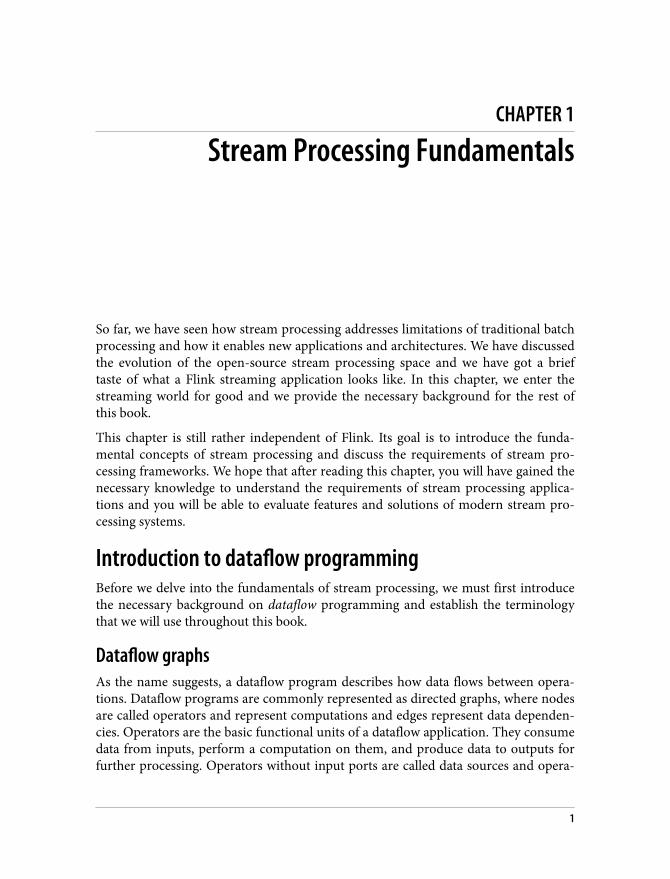
tors without output ports are called data sinks. A dataflow graph must have at leastone data source and one data sink. Figure 2.1 shows a dataflow program that extractsand counts hashtags from an input stream of tweets.

Figure 1-1. A logical dataflow graph to continuously count hashtags. Nodes representoperators and edges denote data dependencies.

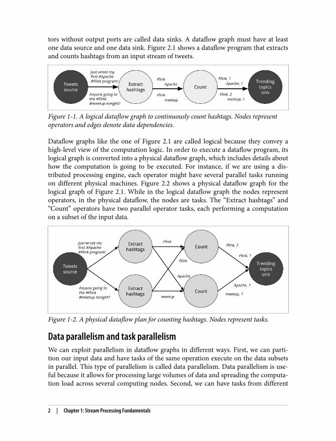
Dataflow graphs like the one of Figure 2.1 are called logical because they convey ahigh-level view of the computation logic. In order to execute a dataflow program, itslogical graph is converted into a physical dataflow graph, which includes details abouthow the computation is going to be executed. For instance, if we are using a dis‐tributed processing engine, each operator might have several parallel tasks runningon different physical machines. Figure 2.2 shows a physical dataflow graph for thelogical graph of Figure 2.1. While in the logical dataflow graph the nodes representoperators, in the physical dataflow, the nodes are tasks. The “Extract hashtags” and“Count” operators have two parallel operator tasks, each performing a computationon a subset of the input data.

Figure 1-2. A physical dataflow plan for counting hashtags. Nodes represent tasks.

Data parallelism and task parallelismWe can exploit parallelism in dataflow graphs in different ways. First, we can parti‐tion our input data and have tasks of the same operation execute on the data subsetsin parallel. This type of parallelism is called data parallelism. Data parallelism is use‐ful because it allows for processing large volumes of data and spreading the computa‐tion load across several computing nodes. Second, we can have tasks from different

2 | Chapter 1: Stream Processing Fundamentals

operators performing computations on the same or different data in parallel. Thistype of parallelism is called task parallelism. Using task parallelism we can better uti‐lize the computing resources of a cluster.

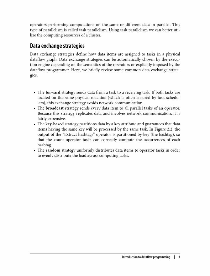
Data exchange strategiesData exchange strategies define how data items are assigned to tasks in a physicaldataflow graph. Data exchange strategies can be automatically chosen by the execu‐tion engine depending on the semantics of the operators or explicitly imposed by thedataflow programmer. Here, we briefly review some common data exchange strate‐gies.

• The forward strategy sends data from a task to a receiving task. If both tasks arelocated on the same physical machine (which is often ensured by task schedu‐lers), this exchange strategy avoids network communication.

• The broadcast strategy sends every data item to all parallel tasks of an operator.Because this strategy replicates data and involves network communication, it isfairly expensive.

• The key-based strategy partitions data by a key attribute and guarantees that dataitems having the same key will be processed by the same task. In Figure 2.2, theoutput of the “Extract hashtags” operator is partitioned by key (the hashtag), sothat the count operator tasks can correctly compute the occurrences of eachhashtag.

• The random strategy uniformly distributes data items to operator tasks in orderto evenly distribute the load across computing tasks.

Introduction to dataflow programming | 3

Figure 1-3. Data exchange strategies.

Processing infinite streams in parallelNow that we have become familiar with the basics of dataflow programming, it’s timeto see how these concepts apply to processing data streams in parallel. But first, wedefine the term data stream:

A data stream is a potentially unbounded sequence of events

Events in a data stream can represent monitoring data, sensor measurements, creditcard transactions, weather station observations, online user interactions, websearches, etc. In this section, we are going to learn the concepts of processing infinitestreams in parallel, using the dataflow programming paradigm.

Latency and throughputIn the previous chapter, we saw how streaming applications have different operationalrequirements from traditional batch programs. Requirements also differ when itcomes to evaluating performance. For batch applications, we usually care about thetotal execution time of a job, or how long it takes for our processing engine to readthe input, perform the computation, and write back the result. Since streaming appli‐


cations run continuously and the input is potentially unbounded, there is no notionof total execution time in data stream processing. Instead, streaming applicationsmust provide results for incoming data as fast as possible while being able to handlehigh ingest rates of events. We express these performance requirements in terms oflatency and throughput.

LatencyLatency indicates how long it takes for an event to be processed. Essentially, it is thetime interval between receiving an event and seeing the effect of processing this eventin the output. To understand latency intuitively, consider your daily visit to yourfavorite coffee shop. When you enter the coffee shop, there might be other customersinside already. Thus, you wait in line and when it is your turn you make an order. Thecashier receives your payment and passes your order to the barista who prepares yourbeverage. Once your coffee is ready, the barista calls your name and you can pick upyour coffee from the bench. Your service latency is the time you spend in the coffeeshop, from the moment you enter until you have the first sip of coffee.

In data streaming, latency is measured in units of time, such as milliseconds. Depend‐ing on the application, we might care about average latency, maximum latency, or per‐centile latency. For example, an average latency value of 10ms means that events areprocessed within 10ms on average. Instead, a 95th-percentile latency value of 10msmeans that 95% of events are processed within 10ms. Average values hide the truedistribution of processing delays and might make it hard to detect problems. If thebarista runs out of milk right before preparing your cappuccino, you will have to waituntil they bring some from the supply room. While you might get annoyed by thisdelay, most other customers will still be happy.

Ensuring low latency is critical for many streaming applications, such as fraud detec‐tion, raising alarms, network monitoring, and offering services with strict servicelevel agreements (SLAs). Low latency is what makes stream processing attractive andenables what we call real-time applications. Modern stream processors, like ApacheFlink, can offer latencies as low as a few milliseconds. In contrast, traditional batchprocessing latencies typically range from a few minutes to several hours. In batchprocessing we first need to gather the events in batches and only then we are able toprocess them. Thus, the latency is bounded by the arrival time of the last event ineach batch and naturally depends on the batch size. True stream processing does notintroduce such artificial delays and therefore can achieve really low latencies. In atrue streaming model, events can be processed as soon as they arrive in the systemand latency reflects the actual work that has to performed on each event.

ThroughputThroughput is a measure of the system’s processing capacity, i.e. its rate of processing.That is, throughput tells us how many events the system can process per time unit.

Processing infinite streams in parallel | 5

Revisiting the coffee shop example, if the shop is open from 7am to 7pm and it serves600 customers in one day, then its average throughput would be 50 customers perhour. While we want latency to be as low as possible, we generally want throughput tobe as high as possible.

Throughput is measured in events or operations per time unit. It is important to notethat the rate of processing depends on the rate of arrival; low throughput does notnecessarily indicate bad performance. In streaming systems we usually want to ensurethat our system can handle the maximum expected rate of events. That is, we are pri‐marily concerned with determining the peak throughput, i.e. the performance limitwhen our system is at its maximum load. To better understand the concept of peakthroughput, let us consider that our system resources are completely unused. As thefirst event comes in, it will be immediately processed with the minimum latency pos‐sible. If you are the first customer showing up at the coffee shop right after it openedits doors in the morning, you will be served immediately. Ideally, we would like thislatency to remain constant and independent of the rate of the incoming events. How‐ever, once we reach a rate of incoming events such that the system resources are fullyused, we will have to start buffering events. In the coffee shop example, you will prob‐ably see this happening right after lunch. Many people show up at the same time andyou have to wait in line to place your order. At this point we have reached the peakthroughput and further increasing the event rate will only result in worse latency. Ifthe system continues to receive data at a higher rate than it can handle, buffers mightbecome unavailable and data might get lost. This situation is commonly known asbackpressure and there exist different strategies to deal with it. In Chapter 3, we lookat Flink’s backpressure mechanism in detail.

Latency vs. throughputAt this point, it should be quite clear that latency and throughput are not independ‐ent metrics. If events take long to travel in the data processing pipeline, we cannoteasily ensure high throughput. Similarly, if a system’s capacity is small, events will bebuffered and have to wait before they get processed.

Let us revisit the coffee shop example to clarify how latency and throughput affecteach other. First, it should be clear that there is an optimal latency in the case of noload. That is, we will get the fastest service if we are the only customer in the coffeeshop. However, during busy times, customers will have to wait in line and latency willincrease. Another factor that affects latency and consequently throughput is the timeit takes to process an event, or the time it takes for each customer to be served in ourcoffee shop. Imagine that during Christmas holiday season, baristas have to draw aSanta Claus on the cup of each coffee they serve. This way, the time to prepare a sin‐gle beverage will increase, causing each person to spend more time in the coffee shop,thus lowering the overall throughput.


Then, can we somehow get both low latency and high throughput or is this a hopelessendeavour? One way we can lower latency is by hiring a more skilled barista, i.e. onethat prepares coffees faster. At high load, this change will also increase throughput,because more customers will be served in the same amount of time. Another way toachieve the same result is to hire a second barista, that is, to exploit parallelism. Themain take-away here is that lowering latency actually increases throughput. Naturally,if a system can perform operations faster, it can perform more operations at the sameamount of time. In fact, that is what we achieve by exploiting parallelism in a streamprocessing pipeline. By processing several streams in parallel, we can lower thelatency while processing more events at the same time.

Operations on data streamsStream processing engines usually provide a set of built-in operations to ingest, trans‐form, and output streams. These operators can be combined into dataflow processinggraphs to implement the logic of streaming applications. In this section, we describethe most common streaming operations.

Operations can be either stateless or stateful. Stateless operations do not maintain anyinternal state. That is, the processing of an event does not depend on any events seenin the past and no history is kept. Stateless operations are easy to parallelize, sinceevents can be processed independently of each other and of their arriving order.Moreover, in the case of a failure, a stateless operator can be simply restarted andcontinue processing from where it left off. On the contrary, stateful operators maymaintain information about the events they have received before. This state can beupdated by incoming events and can be used in the processing logic of future events.Stateful stream processing applications are more challenging to parallelize and oper‐ate in a fault tolerance manner because state needs to be efficiently partitioned andreliably recovered in the case of failures. We further discuss stateful stream process‐ing, failure scenarios, and consistency in the end of this chapter.

Data ingestion and data egressData ingestion and data egress operations allow the stream processor to communicatewith external systems. Data ingestion is the operation of fetching raw data from exter‐nal sources and converting it into a format that is suitable for processing. Operatorsthat implement data ingestion logic are called data sources. A data source can ingestdata from a TCP socket, a file, a Kafka topic, or a sensor data interface. Data egress isthe operation of producing output in a form that is suitable for consumption byexternal systems. Operators that perform data egress are called data sinks and exam‐ples include files, databases, message queues, and monitoring interfaces.


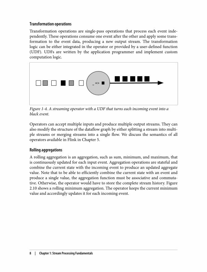
Transformation operationsTransformation operations are single-pass operations that process each event inde‐pendently. These operations consume one event after the other and apply some trans‐formation to the event data, producing a new output stream. The transformationlogic can be either integrated in the operator or provided by a user-defined function(UDF). UDFs are written by the application programmer and implement customcomputation logic.

Figure 1-4. A streaming operator with a UDF that turns each incoming event into ablack event.

Operators can accept multiple inputs and produce multiple output streams. They canalso modify the structure of the dataflow graph by either splitting a stream into multi‐ple streams or merging streams into a single flow. We discuss the semantics of alloperators available in Flink in Chapter 5.

Rolling aggregationsA rolling aggregation is an aggregation, such as sum, minimum, and maximum, thatis continuously updated for each input event. Aggregation operations are stateful andcombine the current state with the incoming event to produce an updated aggregatevalue. Note that to be able to efficiently combine the current state with an event andproduce a single value, the aggregation function must be associative and commuta‐tive. Otherwise, the operator would have to store the complete stream history. Figure2.10 shows a rolling minimum aggregation. The operator keeps the current minimumvalue and accordingly updates it for each incoming event.


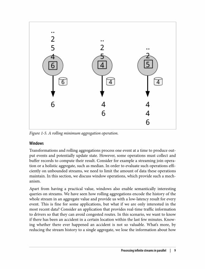
Figure 1-5. A rolling minimum aggregation operation.

WindowsTransformations and rolling aggregations process one event at a time to produce out‐put events and potentially update state. However, some operations must collect andbuffer records to compute their result. Consider for example a streaming join opera‐tion or a holistic aggregate, such as median. In order to evaluate such operations effi‐ciently on unbounded streams, we need to limit the amount of data these operationsmaintain. In this section, we discuss window operations, which provide such a mech‐anism.

Apart from having a practical value, windows also enable semantically interestingqueries on streams. We have seen how rolling aggregations encode the history of thewhole stream in an aggregate value and provide us with a low-latency result for everyevent. This is fine for some applications, but what if we are only interested in themost recent data? Consider an application that provides real-time traffic informationto drivers so that they can avoid congested routes. In this scenario, we want to knowif there has been an accident in a certain location within the last few minutes. Know‐ing whether there ever happened an accident is not so valuable. What’s more, byreducing the stream history to a single aggregate, we lose the information about how


our data varies over time. For instance, we might want to know how many vehiclescross an intersection every 5 minutes.

Window operations continuously create finite sets of events called buckets from anunbounded event stream and let us perform computations on these finite sets. Eventsare usually assigned to buckets based on data properties or based on time. To prop‐erly define window operator semantics, we need to answer two main questions: “howare events assigned to buckets?” and “how often does the window produce a result?”. Thebehavior of windows is defined by a set of policies. Window policies decide when newbuckets are created, which events are assigned to which buckets, and when the con‐tents of a bucket get evaluated. The latter decision is based on a trigger condition.When the trigger condition is met, the bucket contents are sent to an evaluation func‐tion that applies the computation logic on the bucket elements. Evaluation functionscan be aggregations like sum or minimum or custom operations applied on the buck‐et’s collected elements. Policies can be based on time (e.g. events received in the last 5seconds), on count (e.g. the last 100 events), or on a data property. In this section, wedescribe the semantics of common window types.

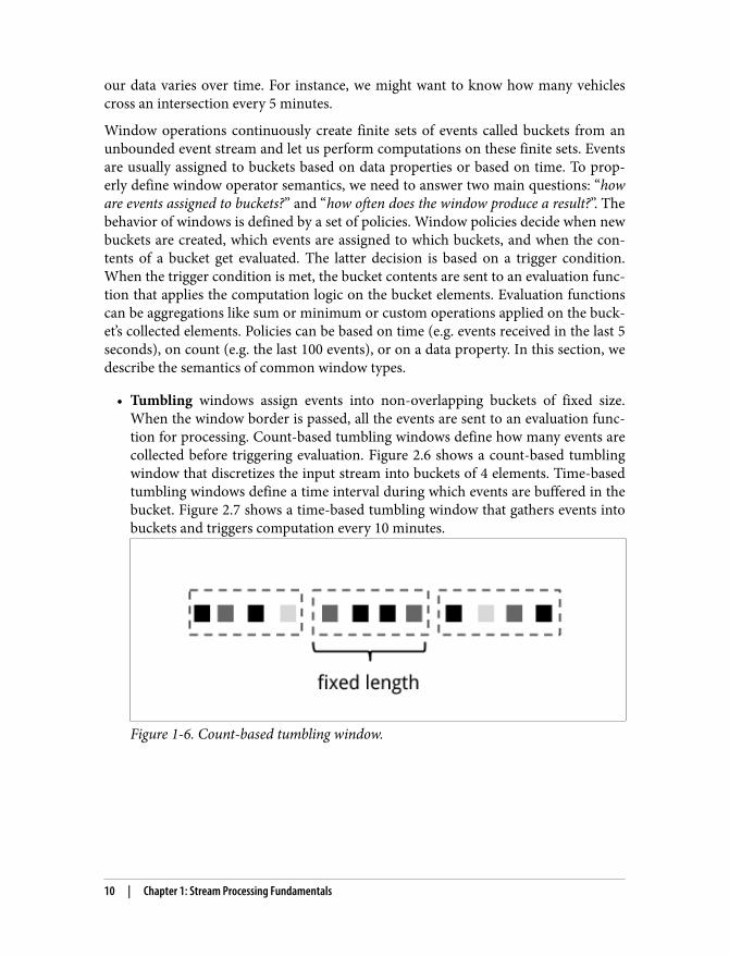
• Tumbling windows assign events into non-overlapping buckets of fixed size.When the window border is passed, all the events are sent to an evaluation func‐tion for processing. Count-based tumbling windows define how many events arecollected before triggering evaluation. Figure 2.6 shows a count-based tumblingwindow that discretizes the input stream into buckets of 4 elements. Time-basedtumbling windows define a time interval during which events are buffered in thebucket. Figure 2.7 shows a time-based tumbling window that gathers events intobuckets and triggers computation every 10 minutes.

Figure 1-6. Count-based tumbling window.


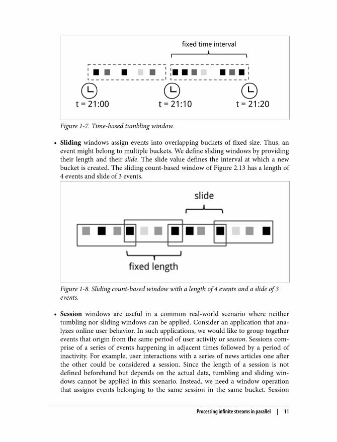
Figure 1-7. Time-based tumbling window.

• Sliding windows assign events into overlapping buckets of fixed size. Thus, anevent might belong to multiple buckets. We define sliding windows by providingtheir length and their slide. The slide value defines the interval at which a newbucket is created. The sliding count-based window of Figure 2.13 has a length of4 events and slide of 3 events.

Figure 1-8. Sliding count-based window with a length of 4 events and a slide of 3events.

• Session windows are useful in a common real-world scenario where neithertumbling nor sliding windows can be applied. Consider an application that ana‐lyzes online user behavior. In such applications, we would like to group togetherevents that origin from the same period of user activity or session. Sessions com‐prise of a series of events happening in adjacent times followed by a period ofinactivity. For example, user interactions with a series of news articles one afterthe other could be considered a session. Since the length of a session is notdefined beforehand but depends on the actual data, tumbling and sliding win‐dows cannot be applied in this scenario. Instead, we need a window operationthat assigns events belonging to the same session in the same bucket. Session


windows group events in session based on a session gap value that defines thetime of inactivity to consider a session closed. Figure 2.9 shows a session window.

Figure 1-9. Session window.

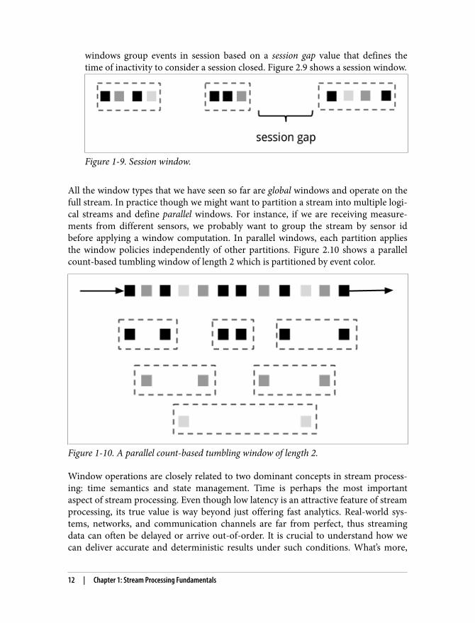
All the window types that we have seen so far are global windows and operate on thefull stream. In practice though we might want to partition a stream into multiple logi‐cal streams and define parallel windows. For instance, if we are receiving measure‐ments from different sensors, we probably want to group the stream by sensor idbefore applying a window computation. In parallel windows, each partition appliesthe window policies independently of other partitions. Figure 2.10 shows a parallelcount-based tumbling window of length 2 which is partitioned by event color.

Figure 1-10. A parallel count-based tumbling window of length 2.

Window operations are closely related to two dominant concepts in stream process‐ing: time semantics and state management. Time is perhaps the most importantaspect of stream processing. Even though low latency is an attractive feature of streamprocessing, its true value is way beyond just offering fast analytics. Real-world sys‐tems, networks, and communication channels are far from perfect, thus streamingdata can often be delayed or arrive out-of-order. It is crucial to understand how wecan deliver accurate and deterministic results under such conditions. What’s more,


streaming applications that process events as they are produced should also be able toprocess historical events in the same way, thus enabling offline analytics or even timetravel analyses. Of course, none of this matters if our system cannot guard stateagainst failures. All the window types that we have seen so far need to buffer databefore performing an operation. In fact, if we want to compute anything interestingin a streaming application, even a simple count, we need to maintain state. Consider‐ing that streaming applications might run for several days, months, or even years, weneed to make sure that state can be reliably recovered under failures and that our sys‐tem can guarantee accurate results even if things break. In the rest of this chapter, weare going to look deeper into the concepts of time and state guarantees under failuresin data stream processing.

Time semanticsIn this section, we introduce time semantics and describe the different notions oftime in streaming. We discuss how a stream processor can provide accurate resultswith out-of-order events and how we can support historical event processing andtime travel with streaming.

What is the meaning of one minute?When dealing with a potentially unbounded stream of continuously arriving events,time becomes a central aspect of applications. Let’s assume we want to computeresults continuously, for example every one minute. What would one minute reallymean in the context of our streaming application?

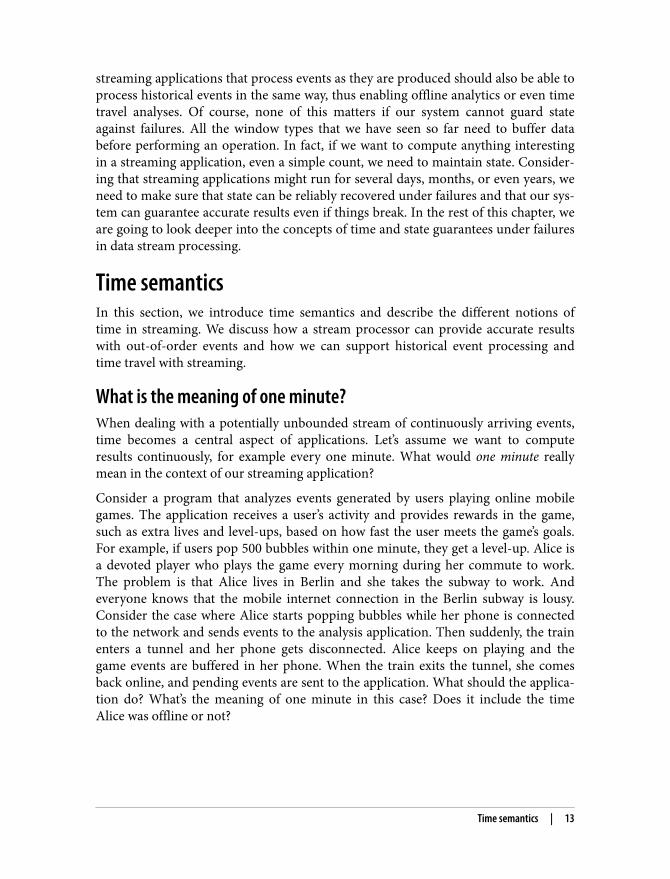
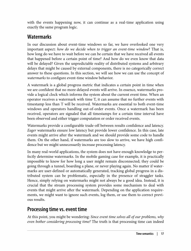
Consider a program that analyzes events generated by users playing online mobilegames. The application receives a user’s activity and provides rewards in the game,such as extra lives and level-ups, based on how fast the user meets the game’s goals.For example, if users pop 500 bubbles within one minute, they get a level-up. Alice isa devoted player who plays the game every morning during her commute to work.The problem is that Alice lives in Berlin and she takes the subway to work. Andeveryone knows that the mobile internet connection in the Berlin subway is lousy.Consider the case where Alice starts popping bubbles while her phone is connectedto the network and sends events to the analysis application. Then suddenly, the trainenters a tunnel and her phone gets disconnected. Alice keeps on playing and thegame events are buffered in her phone. When the train exits the tunnel, she comesback online, and pending events are sent to the application. What should the applica‐tion do? What’s the meaning of one minute in this case? Does it include the timeAlice was offline or not?

Time semantics | 13

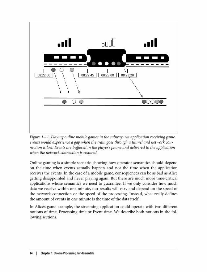
Figure 1-11. Playing online mobile games in the subway. An application receiving gameevents would experience a gap when the train goes through a tunnel and network con‐nection is lost. Events are buffered in the player’s phone and delivered to the applicationwhen the network connection is restored.

Online gaming is a simple scenario showing how operator semantics should dependon the time when events actually happen and not the time when the applicationreceives the events. In the case of a mobile game, consequences can be as bad as Alicegetting disappointed and never playing again. But there are much more time-criticalapplications whose semantics we need to guarantee. If we only consider how muchdata we receive within one minute, our results will vary and depend on the speed ofthe network connection or the speed of the processing. Instead, what really definesthe amount of events in one minute is the time of the data itself.

In Alice’s game example, the streaming application could operate with two differentnotions of time, Processing time or Event time. We describe both notions in the fol‐lowing sections.


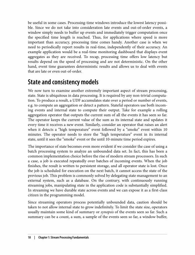
Processing timeProcessing time is the time of the local clock on the machine where the operator pro‐cessing the stream is being executed. A processing-time window includes all eventsthat happen to have arrived at the window operator within a time period, as meas‐ured by the wall-clock of its machine. In Alice’s case, a processing-time windowwould continue counting time when her phone gets disconnected, thus not account‐ing for her game activity during that time:

Figure 1-12. A processing-time window continues counting time when Alice’s phone getsdisconnected.

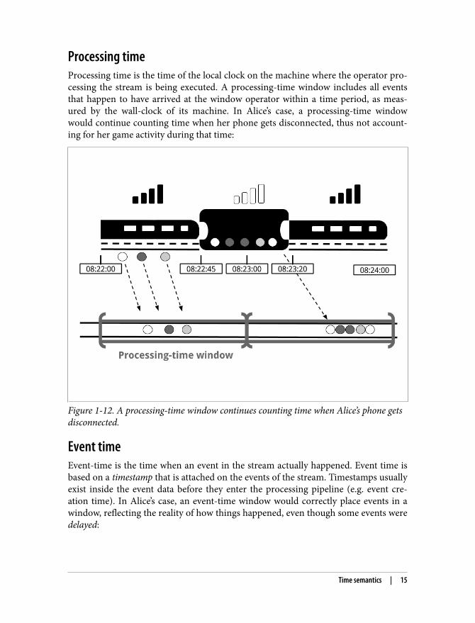
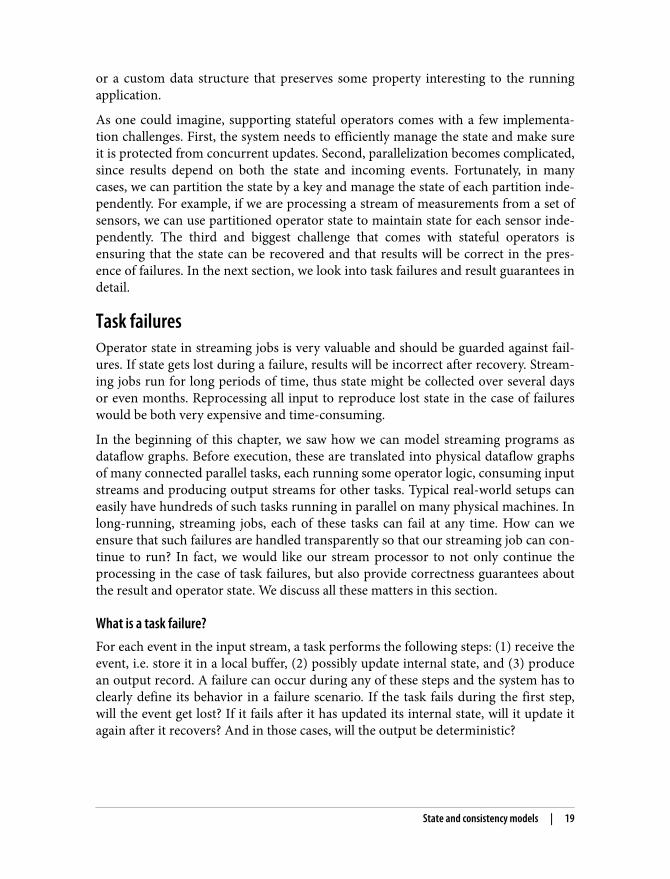
Event timeEvent-time is the time when an event in the stream actually happened. Event time isbased on a timestamp that is attached on the events of the stream. Timestamps usuallyexist inside the event data before they enter the processing pipeline (e.g. event cre‐ation time). In Alice’s case, an event-time window would correctly place events in awindow, reflecting the reality of how things happened, even though some events weredelayed:

Time semantics | 15

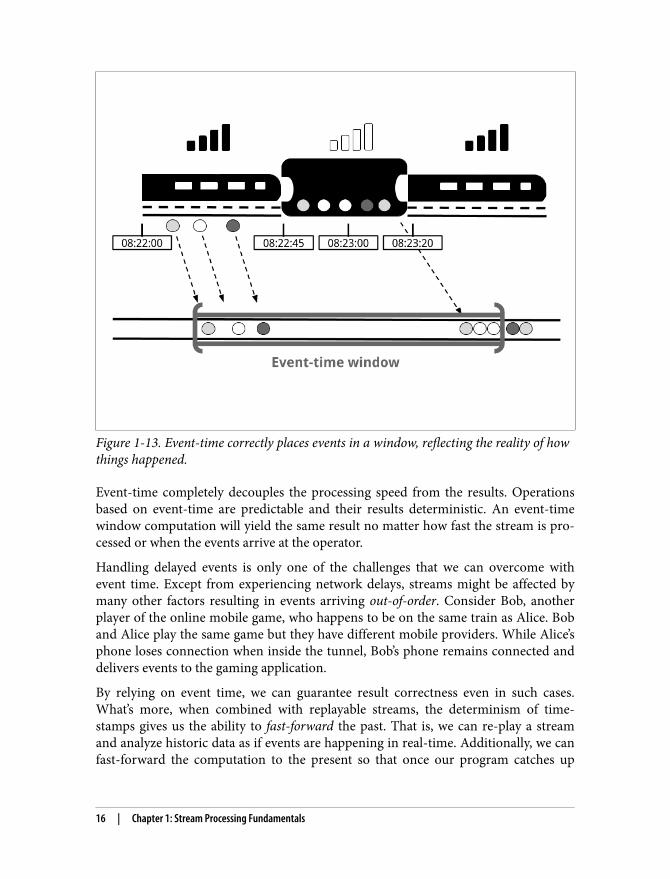
Figure 1-13. Event-time correctly places events in a window, reflecting the reality of howthings happened.

Event-time completely decouples the processing speed from the results. Operationsbased on event-time are predictable and their results deterministic. An event-timewindow computation will yield the same result no matter how fast the stream is pro‐cessed or when the events arrive at the operator.

Handling delayed events is only one of the challenges that we can overcome withevent time. Except from experiencing network delays, streams might be affected bymany other factors resulting in events arriving out-of-order. Consider Bob, anotherplayer of the online mobile game, who happens to be on the same train as Alice. Boband Alice play the same game but they have different mobile providers. While Alice’sphone loses connection when inside the tunnel, Bob’s phone remains connected anddelivers events to the gaming application.

By relying on event time, we can guarantee result correctness even in such cases.What’s more, when combined with replayable streams, the determinism of time‐stamps gives us the ability to fast-forward the past. That is, we can re-play a streamand analyze historic data as if events are happening in real-time. Additionally, we canfast-forward the computation to the present so that once our program catches up


with the events happening now, it can continue as a real-time application usingexactly the same program logic.

WatermarksIn our discussion about event-time windows so far, we have overlooked one veryimportant aspect: how do we decide when to trigger an event-time window? That is,how long do we have to wait before we can be certain that we have received all eventsthat happened before a certain point of time? And how do we even know that datawill be delayed? Given the unpredictable reality of distributed systems and arbitrarydelays that might be caused by external components, there is no categorically correctanswer to these questions. In this section, we will see how we can use the concept ofwatermarks to configure event-time window behavior.

A watermark is a global progress metric that indicates a certain point in time whenwe are confident that no more delayed events will arrive. In essence, watermarks pro‐vide a logical clock which informs the system about the current event time. When anoperator receives a watermark with time T, it can assume that no further events withtimestamp less than T will be received. Watermarks are essential to both event-timewindows and operators handling out-of-order events. Once a watermark has beenreceived, operators are signaled that all timestamps for a certain time interval havebeen observed and either trigger computation or order received events.

Watermarks provide a configurable trade-off between results confidence and latency.Eager watermarks ensure low latency but provide lower confidence. In this case, lateevents might arrive after the watermark and we should provide some code to handlethem. On the other hand, if watermarks are too slow to arrive, we have high confi‐dence but we might unnecessarily increase processing latency.

In many real-world applications, the system does not have enough knowledge to per‐fectly determine watermarks. In the mobile gaming case for example, it is practicallyimpossible to know for how long a user might remain disconnected; they could begoing through a tunnel, boarding a plane, or never playing again. No matter if water‐marks are user-defined or automatically generated, tracking global progress in a dis‐tributed system can be problematic, especially in the presence of straggler tasks.Hence, simply relying on watermarks might not always be a good idea. Instead, it iscrucial that the stream processing system provides some mechanism to deal withevents that might arrive after the watermark. Depending on the application require‐ments, we might want to ignore such events, log them, or use them to correct previ‐ous results.

Processing time vs. event timeAt this point, you might be wondering: Since event time solves all of our problems, whyeven bother considering processing time? The truth is that processing time can indeed

Time semantics | 17

be useful in some cases. Processing-time windows introduce the lowest latency possi‐ble. Since we do not take into consideration late events and out-of-order events, awindow simply needs to buffer up events and immediately trigger computation oncethe specified time length is reached. Thus, for applications where speed is moreimportant than accuracy, processing time comes handy. Another case is when weneed to periodically report results in real-time, independently of their accuracy. Anexample application would be a real-time monitoring dashboard that displays eventaggregates as they are received. To recap, processing time offers low latency butresults depend on the speed of processing and are not deterministic. On the otherhand, event time guarantees deterministic results and allows us to deal with eventsthat are late or even out-of-order.

State and consistency modelsWe now turn to examine another extremely important aspect of stream processing,state. State is ubiquitous in data processing. It is required by any non-trivial computa‐tion. To produce a result, a UDF accumulates state over a period or number of events,e.g. to compute an aggregation or detect a pattern. Stateful operators use both incom‐ing events and internal state to compute their output. Take for example a rollingaggregation operator that outputs the current sum of all the events it has seen so far.The operator keeps the current value of the sum as its internal state and updates itevery time it receives a new event. Similarly, consider an operator that raises an alertwhen it detects a “high temperature” event followed by a “smoke” event within 10minutes. The operator needs to store the “high temperature” event in its internalstate, until it sees the “smoke” event or the until 10-minute time period expires.

The importance of state becomes even more evident if we consider the case of using abatch processing system to analyze an unbounded data set. In fact, this has been acommon implementation choice before the rise of modern stream processors. In sucha case, a job is executed repeatedly over batches of incoming events. When the jobfinishes, the result is written to persistent storage, and all operator state is lost. Oncethe job is scheduled for execution on the next batch, it cannot access the state of theprevious job. This problem is commonly solved by delegating state management to anexternal system, such as a database. On the contrary, with continuously runningstreaming jobs, manipulating state in the application code is substantially simplified.In streaming we have durable state across events and we can expose it as a first-classcitizen in the programming model.

Since streaming operators process potentially unbounded data, caution should betaken to not allow internal state to grow indefinitely. To limit the state size, operatorsusually maintain some kind of summary or synopsis of the events seen so far. Such asummary can be a count, a sum, a sample of the events seen so far, a window buffer,


or a custom data structure that preserves some property interesting to the runningapplication.

As one could imagine, supporting stateful operators comes with a few implementa‐tion challenges. First, the system needs to efficiently manage the state and make sureit is protected from concurrent updates. Second, parallelization becomes complicated,since results depend on both the state and incoming events. Fortunately, in manycases, we can partition the state by a key and manage the state of each partition inde‐pendently. For example, if we are processing a stream of measurements from a set ofsensors, we can use partitioned operator state to maintain state for each sensor inde‐pendently. The third and biggest challenge that comes with stateful operators isensuring that the state can be recovered and that results will be correct in the pres‐ence of failures. In the next section, we look into task failures and result guarantees indetail.

Task failuresOperator state in streaming jobs is very valuable and should be guarded against fail‐ures. If state gets lost during a failure, results will be incorrect after recovery. Stream‐ing jobs run for long periods of time, thus state might be collected over several daysor even months. Reprocessing all input to reproduce lost state in the case of failureswould be both very expensive and time-consuming.

In the beginning of this chapter, we saw how we can model streaming programs asdataflow graphs. Before execution, these are translated into physical dataflow graphsof many connected parallel tasks, each running some operator logic, consuming inputstreams and producing output streams for other tasks. Typical real-world setups caneasily have hundreds of such tasks running in parallel on many physical machines. Inlong-running, streaming jobs, each of these tasks can fail at any time. How can weensure that such failures are handled transparently so that our streaming job can con‐tinue to run? In fact, we would like our stream processor to not only continue theprocessing in the case of task failures, but also provide correctness guarantees aboutthe result and operator state. We discuss all these matters in this section.

What is a task failure?For each event in the input stream, a task performs the following steps: (1) receive theevent, i.e. store it in a local buffer, (2) possibly update internal state, and (3) producean output record. A failure can occur during any of these steps and the system has toclearly define its behavior in a failure scenario. If the task fails during the first step,will the event get lost? If it fails after it has updated its internal state, will it update itagain after it recovers? And in those cases, will the output be deterministic?

State and consistency models | 19

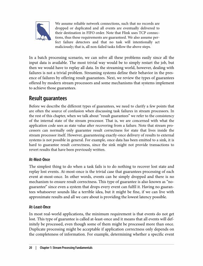
We assume reliable network connections, such that no records aredropped or duplicated and all events are eventually delivered totheir destination in FIFO order. Note that Flink uses TCP connec‐tions, thus these requirements are guaranteed. We also assume per‐fect failure detectors and that no task will intentionally actmaliciously; that is, all non-failed tasks follow the above steps.

In a batch processing scenario, we can solve all these problems easily since all theinput data is available. The most trivial way would be to simply restart the job, butthen we would have to replay all data. In the streaming world, however, dealing withfailures is not a trivial problem. Streaming systems define their behavior in the pres‐ence of failures by offering result guarantees. Next, we review the types of guaranteesoffered by modern stream processors and some mechanisms that systems implementto achieve those guarantees.

Result guaranteesBefore we describe the different types of guarantees, we need to clarify a few points thatare often the source of confusion when discussing task failures in stream processors. Inthe rest of this chapter, when we talk about “result guarantees” we refer to the consistencyof the internal state of the stream processor. That is, we are concerned with what theapplication code sees as state value after recovering from a failure. Note that stream pro‐cessors can normally only guarantee result correctness for state that lives inside thestream processor itself. However, guaranteeing exactly-once delivery of results to externalsystems is not possible in general. For example, once data has been emitted to a sink, it ishard to guarantee result correctness, since the sink might not provide transactions torevert results that have been previously written.

At-Most-OnceThe simplest thing to do when a task fails is to do nothing to recover lost state andreplay lost events. At-most-once is the trivial case that guarantees processing of eachevent at-most-once. In other words, events can be simply dropped and there is nomechanism to ensure result correctness. This type of guarantee is also known as “no-guarantee” since even a system that drops every event can fulfil it. Having no guaran‐tees whatsoever sounds like a terrible idea, but it might be fine, if we can live withapproximate results and all we care about is providing the lowest latency possible.

At-Least-OnceIn most real-world applications, the minimum requirement is that events do not getlost. This type of guarantee is called at-least-once and it means that all events will def‐initely be processed, even though some of them might be processed more than once.Duplicate processing might be acceptable if application correctness only depends onthe completeness of information. For example, determining whether a specific event


occurs in the input stream can be correctly realized with at-least-once guarantees. Inthe worst case, we will locate the event more than once. However, counting howmany times a specific event occurs in the input stream might return the wrong resultunder at-least-once guarantees.

In order to ensure at-least-once result correctness, we need to have a mechanism toreplay events, either from the source or from some buffer. Persistent event logs writeall events to durable storage, so that they can be replayed if a task fails. Another wayto achieve equivalent functionality is using record acknowledgements. This methodstores every event in a buffer until its processing has been acknowledged by all tasksin the pipeline, at which point the event can be discarded.

Exactly-OnceThis is the strictest and most challenging to achieve type of guarantee. Exactly-onceresult guarantees means that not only there will be no event loss, but also updates onthe internal state will be applied exactly once for each event. In essence, exactly-onceguarantees mean that our application will provide the correct result, as if a failurenever happened.

Providing exactly-once guarantees requires at-least-once guarantees, thus a datareplay mechanism is again necessary. Additionally, the stream processor needs toensure internal state consistency. That is, after recovery, it should know whether anevent update has already been reflected on the state or not. Transactional updates isone way to achieve this result, however, it can incur substantial performance over‐head. Instead, Flink uses a lightweight snapshotting mechanism to achieve exactly-once result guarantees. We discuss Flink’s fault-tolerance algorithm in Chapter 3.

End-to-end Exactly-OnceThe types of guarantees we have seen so far refer to the stream processor componentonly. In a real-word streaming architecture however, it is common to have severalconnected components. In the very simple case, there will be at least one source andone sink apart from the stream processor. End-to-end guarantees refer to result cor‐rectness across the data processing pipeline. To assess end-to-end guarantees, one hasto consider all the components of an application pipeline. Each component providesits own guarantees and the end-to-end guarantee of the complete pipeline would bethe weakest of each of its components. It is important to note that sometimes we canget stronger semantics with weaker guarantees. A common case is when a task per‐forms idempotent operations, like maximum or minimum. In this case, we can ach‐ieve exactly-once semantics with at-least-once guarantees.

State and consistency models | 21

SummaryIn this chapter, we have introduced data stream processing by describing fundamen‐tal concepts and ideas. We have explained the dataflow programming model and wehave shown how streaming applications can be expressed as distributed dataflowgraphs. Next, we have looked into the requirements of processing infinite streams inparallel and we have discussed the importance of latency and throughput for streamapplications. We have introduced basic streaming operations and we have showedhow we can compute meaningful results on unbounded input data using windows.We have wondered about the meaning of time in stream processing and we havecompared the notions of event time and processing time. Finally, we have seen whystate is important in streaming applications and how we can guard it against failuresand guarantee correct results.

Up to this point, we have considered streaming concepts independently of ApacheFlink. In the rest of this book, we are going to see how Flink actually implementsthese concepts and how you can use its DataStream APIs to write applications thatuse all of the features that we have introduced so far.


1 see discussion of highly-available setups later in this chapter.

CHAPTER 2

The Architecture of Apache Flink

The previous chapter discussed important concepts of distributed stream processing,such as parallelization, time, and state. In this chapter we give a high-level introduc‐tion into Flink’s architecture and describe how Flink addresses the aspects of streamprocessing that we discussed before. In particular, we explain how Flink is able toprovide low latency and high throughput processing, how it handles time in stream‐ing applications, and how its fault tolerance mechanism works. This chapter providesrelevant background information to successfully implement and operate advancedstreaming applications with Apache Flink. It will help you to understand Flink’s inter‐nals and to reason about the performance and behavior of streaming applications.

System ArchitectureFlink’s architecture follows the master-worker pattern implemented by many dis‐tributed systems. In Flink, the master process is called JobManager1 and a worker pro‐cess is called TaskManager. A Flink cluster consists of at least one JobManager andone or more TaskManagers. Client processes submit applications to the JobManager.Every process runs in a separate Java Virtual Machine (JVM).

Executing an Application Step-by-StepThe responsibilities of the JobManager, TaskManagers, and Client processes are bestexplained by describing the execution of a streaming application at a high level. Thefollowing figure shows the steps of submitting and executing a streaming applicationon Flink.

23

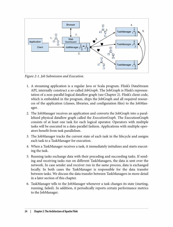
Figure 2-1. Job Submission and Execution.

1. A streaming application is a regular Java or Scala program. Flink’s DataStreamAPI, internally construct a so-called JobGraph. The JobGraph is Flink’s represen‐tation of a non-parallel logical dataflow graph (see Chapter 2). Flink’s client code,which is embedded in the program, ships the JobGraph and all required resour‐ces of the application (classes, libraries, and configuration files) to the JobMan‐ager.

2. The JobManager receives an application and converts the JobGraph into a paral‐lelized physical dataflow graph called the ExecutionGraph. The ExecutionGraphconsists of at least one task for each logical operator. Operators with multipletasks will be executed in a data-parallel fashion. Applications with multiple oper‐ators benefit from task parallelism.

3. The JobManager tracks the current state of each task in the lifecycle and assignseach task to a TaskManager for execution.

4. When a TaskManager receives a task, it immediately initializes and starts execut‐ing the task.

5. Running tasks exchange data with their preceding and succeeding tasks. If send‐ing and receiving tasks run on different TaskManagers, the data is sent over thenetwork. In case sender and receiver run in the same process, data is exchangedlocally. In both cases the TaskManager is responsible for the data transferbetween tasks. We discuss the data transfer between TaskManagers in more detailin a later section of this chapter.

6. TaskManager tells to the JobManager whenever a task changes its state (starting,running, failed). In addition, it periodically reports certain performance metricsto the JobManager.

24 | Chapter 2: The Architecture of Apache Flink

7. Flink’s web dashboard runs as part of the JobManager and publishes details aboutcurrently running or terminated applications. The JobManager exposes the sameinformation also via a REST interface.

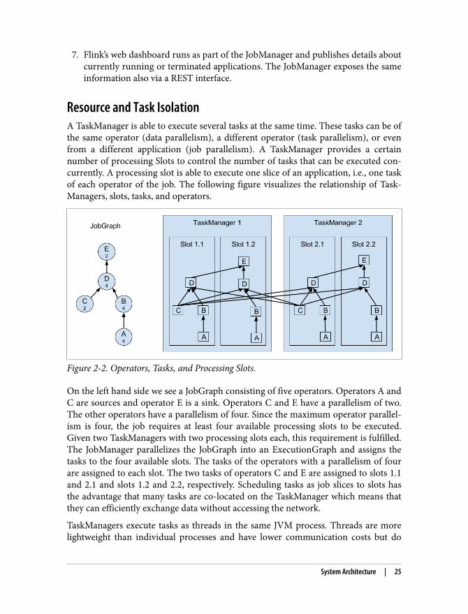
Resource and Task IsolationA TaskManager is able to execute several tasks at the same time. These tasks can be ofthe same operator (data parallelism), a different operator (task parallelism), or evenfrom a different application (job parallelism). A TaskManager provides a certainnumber of processing Slots to control the number of tasks that can be executed con‐currently. A processing slot is able to execute one slice of an application, i.e., one taskof each operator of the job. The following figure visualizes the relationship of Task‐Managers, slots, tasks, and operators.

Figure 2-2. Operators, Tasks, and Processing Slots.

On the left hand side we see a JobGraph consisting of five operators. Operators A andC are sources and operator E is a sink. Operators C and E have a parallelism of two.The other operators have a parallelism of four. Since the maximum operator parallel‐ism is four, the job requires at least four available processing slots to be executed.Given two TaskManagers with two processing slots each, this requirement is fulfilled.The JobManager parallelizes the JobGraph into an ExecutionGraph and assigns thetasks to the four available slots. The tasks of the operators with a parallelism of fourare assigned to each slot. The two tasks of operators C and E are assigned to slots 1.1and 2.1 and slots 1.2 and 2.2, respectively. Scheduling tasks as job slices to slots hasthe advantage that many tasks are co-located on the TaskManager which means thatthey can efficiently exchange data without accessing the network.

TaskManagers execute tasks as threads in the same JVM process. Threads are morelightweight than individual processes and have lower communication costs but do

System Architecture | 25

2 Batch applications can as well exchange data in a bulk fashion. In batch mode, the outgoing data is collected atthe sender and transmitted as a batch over a temporary TCP connection to the receiver.

not strictly isolate tasks from each other. Hence, a single misbehaving task can kill thewhole TaskManager process and all tasks which are being executed on the TaskMan‐ager. Flink features flexible deployment configurations and first class integration withcluster resource managers such as YARN and Apache Mesos (see Chapter X). There‐fore, it is possible to isolate jobs by starting a Flink cluster per job or configuring mul‐tiple TaskManagers with a single processing slot per physical machine. By leveragingthread-parallelism inside of a TaskManager and the option to deploy several Task‐Manager processes per host, Flink offers a lot of flexibility to trade-of performanceand resources isolation when deploying applications. We will discuss the configura‐tion and setup of Flink clusters in detail in Chapter X.

The Networking LayerIn a running streaming application, processing tasks are continuously exchangingdata. The TaskManagers take care of shipping data from sending tasks to receivingtasks. Although Flink is often perceived as a record-at-a-time streaming engine, thecommunication between tasks uses buffers to collect records before they are shippedto achieve satisfying throughput. This batching technique is basically the same mech‐anism as found in networking or disk IO protocols. Each TaskManager has a pool ofbyte buffers (by default 32KB in size) which are used to send and receive data.

If the sender task and receiver task run in the same TaskManager process, the sendertask serializes the outgoing records into a byte buffer and puts the buffer into a queueonce it is filled. The receiving task takes the buffer from the queue and deserializesthe incoming records. Hence, no network communication is involved.

If the sender and receiver tasks run in separate TaskManager processes, the commu‐nication happens via the network stack of the operating system. For streaming appli‐cations, the data exchange must happen in a pipelined fashion, i.e., each pair ofTaskManagers maintains a permanent TCP connection to exchange data 2. In case ofa shuffle connection pattern, each sender task needs to be able to send data to eachreceiving task. A TaskManager that executes a sender task needs for each receivingtask one byte buffer into which the sender task serializes its outgoing data. Once abuffer is filled, it is shipped via the network to the receiving task. On the receiver side,a TaskManager needs one byte buffer for each receiving task. The following figurevisualizes this architecture.


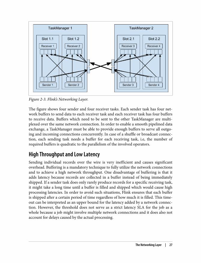
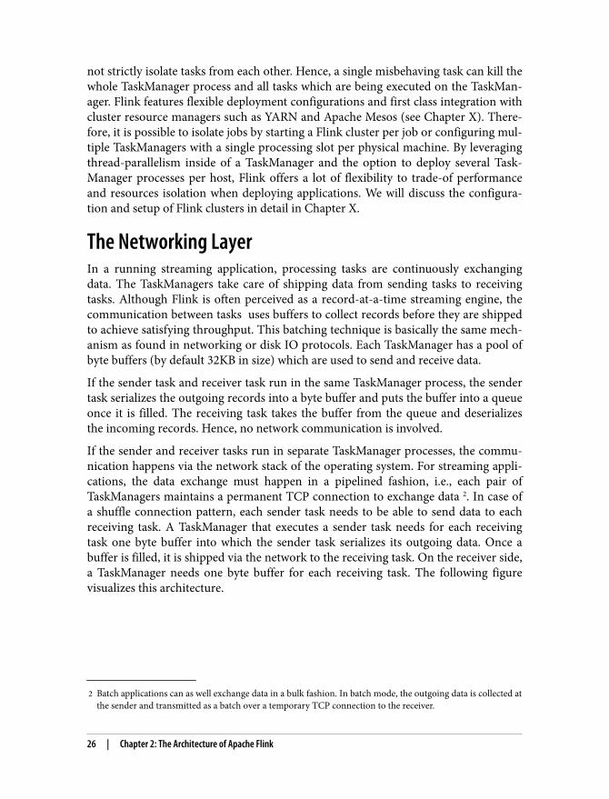
Figure 2-3. Flink’s Networking Layer.

The figure shows four sender and four receiver tasks. Each sender task has four net‐work buffers to send data to each receiver task and each receiver task has four buffersto receive data. Buffers which need to be sent to the other TaskManager are multi‐plexed over the same network connection. In order to enable a smooth pipelined dataexchange, a TaskManager must be able to provide enough buffers to serve all outgo‐ing and incoming connections concurrently. In case of a shuffle or broadcast connec‐tion, each sending task needs a buffer for each receiving task, i.e, the number ofrequired buffers is quadratic to the parallelism of the involved operators.

High Throughput and Low LatencySending individual records over the wire is very inefficient and causes significantoverhead. Buffering is a mandatory technique to fully utilize the network connectionsand to achieve a high network throughput. One disadvantage of buffering is that itadds latency because records are collected in a buffer instead of being immediatelyshipped. If a sender task does only rarely produce records for a specific receiving task,it might take a long time until a buffer is filled and shipped which would cause highprocessing latencies. In order to avoid such situations, Flink ensures that each bufferis shipped after a certain period of time regardless of how much it is filled. This time‐out can be interpreted as an upper bound for the latency added by a network connec‐tion. However, the threshold does not serve as a strict latency SLA for the job as awhole because a job might involve multiple network connections and it does also notaccount for delays caused by the actual processing.

The Networking Layer | 27

Flow Control with Back PressureStreaming applications which ingest streams with high volume can easily come to apoint where a task is not able to process its input data at the rate at which it arrives.This might happen if the volume of an input stream is too high for the amount ofresources allocated to a certain operator or if the input rate of a stream significantlyvaries and causes spikes of high load. Regardless of the reason why an operator can‐not handle its input, this situation should never be a reason for a stream processor toterminate an application. Instead the stream processor should gracefully throttle therate at which a streaming application ingests its input to the maximum speed atwhich the application can process the data. With a decent monitoring infrastructurein place, a throttling situation can be easily detected and usually resolved by addingmore compute resources and increasing the parallelism of the bottleneck operator.The described flow control technique is called backpressure and an important featureof stream processors.

Flink naturally supports backpressure due to the design of its network layer. The fol‐lowing figure illustrates the behavior of the network stack when a receiving task is notable to process its input data at the rate at which it is emitted by the sender task.

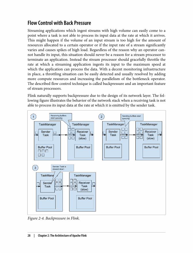
Figure 2-4. Backpressure in Flink.


3 A TaskManager ensures that each task has at least one incoming and one outgoing buffer and respects addi‐tional buffer assignment constraints to avoid deadlocks and maintain smooth communication.

The figure shows a sender and a receiver task running on different machines. (1)When the input rate of the application increases, the sender task can cope with theload but the receiver task starts to fall behind and is no longer able to handle its inputload. Now the receiving TaskManager starts to queue buffers with received data. Atsome point the buffer pool of the receiving TaskManager is empty 3 and can no longercontinue to buffer arriving data. (2) Next, the sending TaskManager starts queuingbuffers with outgoing records until its own buffer pool is empty. (3) Finally, thesender task cannot emit anymore data and blocks until a new buffer becomes avail‐able. A task which is blocked due to a slow receiver behaves itself like a slow receiverand in turn slows down its predecessors. The slowdown escalates up to the sources ofthe streaming application. Eventually, the whole application is slowed down to theprocessing rate of the slowest operator.

Due to the flexible assignment of network buffers to queue outgoing or incomingdata, Flink is able to handle temporary load spikes or slowed down tasks in a verygraceful manner.

Handling Event TimeIn Chapter 2, we highlighted the importance of time semantics for stream processingapplications and explained the differences between processing time and event time.While processing time is easy to understand because it is based on the local time ofthe processing machine, it produces somewhat arbitrary, inconsistent, and non-reproducible results. In contrast, event time semantics yield reproducible and consis‐tent results which is a hard requirement for many stream processing use-cases.However, event-time applications require some additional configuration compared toapplications with processing-time semantics. Also the internals of stream processorsthat support event-time are more involved than the internals of a system that purelyoperates in processing-time. Flink provides intuitive and easy-to-use primitives forcommon event-time processing use cases but also allows implementing moreadvanced event-time applications with custom operators. For such advanced applica‐tions, a good understanding of Flink’s internals is often helpful and sometimes alsorequired. The previous chapter introduced two concepts that Flink leverages to pro‐vide event-time semantics: record timestamps and watermarks. In the following wewill describe how Flink internally implements and handles timestamps and water‐marks to support streaming applications with event-time semantics.

Handling Event Time | 29

TimestampsA Flink streaming application with event-time semantics must ensure that everyrecord has a timestamp. The timestamp associates a record with a specific point intime. Although the semantics of the timestamps are up to the application, they oftenencode the time at which an event happened. When processing a data stream inevent-time mode, Flink evaluates time-based operators based on the timestamps ofrecords. For example, a time-based window operator assigns records to windowsaccording to their associated timestamp. Flink encodes timestamps as 16-byte longvalues and attaches them as metadata to records. Its built-in operators interpret thelong value as a Unix timestamp with millisecond precision, i.e., the number of milli‐seconds since 1970-01-01-00:00:00.000. However, custom operators can have theirown interpretation and, for example, adjust the precision to microseconds.

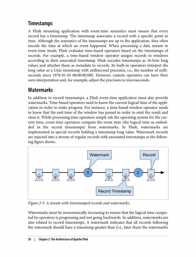
WatermarksIn addition to record timestamps, a Flink event-time application must also providewatermarks. Time-based operators need to know the current logical time of the appli‐cation in order to make progress. For instance, a time-based window operator needsto know that the end-time of the window has passed in order to emit the result andclose it. While processing time operators simply ask the operating system for the cur‐rent time, event-time operators compute the event time (the logical time as embed‐ded in the record timestamps) from watermarks. In Flink, watermarks areimplemented as special records holding a timestamp long value. Watermark recordsare injected into a stream of regular records with annotated timestamps as the follow‐ing figure shows.

Figure 2-5. A stream with timestamped records and watermarks.

Watermarks must be monotonically increasing to ensure that the logical time compu‐ted by operators is progressing and not going backwards. In addition, watermarks arealso related to record timestamps. A watermark indicates that all records followingthe watermark should have a timestamp greater than (i.e., later than) the watermark’s


4 In fact this is a bit oversimplified. Watermarks can be used to control result completeness and latency. We willdiscuss this property of watermarks in Chapter X.

5 The syntax of these functions is discussed in Chapter X.

timestamp 4. Records that violate this condition are so-called late records. When anoperator advances its logical time to the latest watermark and therefore triggers acomputation, late records do not contribute to the result of the computation whichconsequently will be inaccurate or incomplete. Flink provides mechanisms to prop‐erly handle late records. We will discuss these features later in Chapter 6. The require‐ment of monotonically increasing watermarks and the objective to limit the numberof late elements does also mean that the timestamps of the records in a stream shouldbe in general increasing as well. Monotonically increasing timestamps are notrequired though because watermarks are a mechanism to tolerate records with out-of-order timestamps, such as the records with timestamps 3 and 5 in the above figure.

Extraction and Assignment of Timestamps and WatermarksTimestamps and watermarks can be interpreted as properties of a data stream. Theyare usually generated when a stream is ingested by a streaming application. Sincerecord timestamps and watermarks are tightly related with each other, extracting andassigning timestamps and watermarks goes hand in hand in Flink. A Flink applica‐tion can assign timestamps and watermarks in two ways.

The first option is a data source that immediately attaches timestamps and emitswatermarks when ingesting a data stream into the application. This approach ismainly applicable for custom data source functions because timestamp extractiondepends on the often custom data type of a source function. Flink’s built-in connec‐tors are usually more generic and do not extract and assign timestamps and water‐marks (see Chapter X for details on connectors).

The second and more common approach is to use a so-called timestamp and water‐mark extraction operator. The operator is usually applied immediately after a sourcefunction and consists of two user-defined functions5. The first function extracts atimestamp from a record. Flink calls the timestamp extraction function for eachrecord and attaches the extracted long value as metadata to the record. The secondfunction generates a watermark and there are two ways to do this:

1. Generation of periodic watermarks: Flink periodically asks the user-defined func‐tion for the current watermark timestamp. The polling interval can be config‐ured.

2. Generation of punctuated watermarks: Flink calls the user-defined function foreach passing record. The user-defined function may or may not extract a water‐

Handling Event Time | 31

6 The Process operator is invoked per record and gives access to the record’s timestamp, the current watermark,and allows to register timers which invoke a callback function once the time is reached. The Process functionis later discussed in Chapter X.

mark from the record. Punctuated watermarks are useful if the stream containsspecial records that encode watermark information.

In both cases, Flink injects the watermarks returned by the function into the stream. Atimestamp and watermark extractor operator can also be used to override existing time‐stamps and watermarks, for example timestamps and watermarks generated by a sourcefunction. However, it should be noted that this is usually not a good idea and should bedone very carefully.

Handling of Timestamps and WatermarksOnce timestamps have been assigned and watermarks have been generated and injec‐ted into a stream, subsequent operators can process the records of the stream withevent-time semantics. Except for the Process operator6, all built-in operators of Flink’sDataStream API handle timestamps and watermarks internally and do not give devel‐opers access to them. None of the built-in operators (except for timestamp extractorsand watermark generators which were discussed before) expose APIs to adjust orchange timestamps or watermarks.

Instead, the operators take care of maintaining and emitting record timestamps andwatermarks. Some operators have to adjust timestamps of existing records or com‐pute timestamps for new records. For instance, a time window operator attaches theend time of a window as timestamp to all records emitted by the window and subse‐quently forwards the watermarks that triggered the window’s computation. By han‐dling record timestamps and watermarks internally, developers of Flink event-timeapplications only have to provide streams with annotated timestamps and water‐marks and Flink’s operators will take care of everything else.

Computing Event Time from WatermarksFlink is a distributed system and executes streaming applications in a data parallelfashion (see Chapter 2) by splitting streams into stream partitions which are concur‐rently processed. Streams are usually ingested by multiple concurrently runningsource tasks in order to achieve the required throughput. Consequently, watermarksare generated in parallel as well. However, parallel watermark generators do onlyobserve the record timestamps of their local stream partition such that a single water‐mark can only define the logical time in its local partition of the stream.

As mentioned before, watermarks are implemented by Flink as special records whichare received and emitted by operators. Watermarks emitted by an operator task are


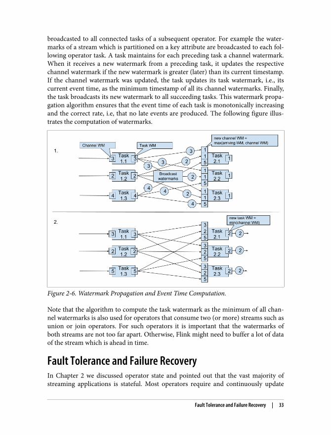
broadcasted to all connected tasks of a subsequent operator. For example the water‐marks of a stream which is partitioned on a key attribute are broadcasted to each fol‐lowing operator task. A task maintains for each preceding task a channel watermark.When it receives a new watermark from a preceding task, it updates the respectivechannel watermark if the new watermark is greater (later) than its current timestamp.If the channel watermark was updated, the task updates its task watermark, i.e., itscurrent event time, as the minimum timestamp of all its channel watermarks. Finally,the task broadcasts its new watermark to all succeeding tasks. This watermark propa‐gation algorithm ensures that the event time of each task is monotonically increasingand the correct rate, i.e, that no late events are produced. The following figure illus‐trates the computation of watermarks.

Figure 2-6. Watermark Propagation and Event Time Computation.

Note that the algorithm to compute the task watermark as the minimum of all chan‐nel watermarks is also used for operators that consume two (or more) streams such asunion or join operators. For such operators it is important that the watermarks ofboth streams are not too far apart. Otherwise, Flink might need to buffer a lot of dataof the stream which is ahead in time.

Fault Tolerance and Failure RecoveryIn Chapter 2 we discussed operator state and pointed out that the vast majority ofstreaming applications is stateful. Most operators require and continuously update

Fault Tolerance and Failure Recovery | 33

some kind of state such as records collected in a window, reading positions of aninput source, or custom, application-specific operator state. In Flink, all state -regardless of built-in or custom operators - is treated the same. Each task manages itsown state and does not share it with other tasks (belonging to the same or other oper‐ators). The state is locally stored on the processing machine, i.e., Flink does not relyon some kind of global mutable state. Since operator state must never be lost, Flinkneeds to protect it from any kinds of failures which are common in distributed sys‐tems such as killed processes, failing machines, and interrupted network connections.For streaming applications with strict latency requirements, the overhead of prepar‐ing for failures as well as recovering from them needs to be low.

Flink’s approach to recover applications and the state of their operators from failuresis based on consistent checkpoints of the complete state of an application. This tech‐nique can provide exactly-once result guarantees. Flink implements a sophisticatedand lightweight algorithm to take consistent checkpoints by copying local operatorstate to a remote storage in a distributed and asynchronous fashion. Moreover, Flinkcan be configured to operate in a highly-available cluster mode without a single pointof failure to be able to tolerate JobManager and TaskManager failures.

In the following sections, we discuss how Flink internally manages state. We explainwhat a consistent checkpoint is and how it is used to recover from failures. We dis‐cuss Flink’s checkpointing algorithm in detail and finally explain how Flink’s highly-available mode works.

State BackendsDuring regular processing, the tasks of a stateful application need efficient read andwrite access to their state. Therefore, tasks locally store their state on their TaskMan‐ager for fast access. However as in any distributed system, TaskManagers may fail atany point in time such that their storage must be considered as volatile. Therefore,Flink periodically checkpoints the local operator state to a remote and persistent stor‐age.

There are different options how operator state can be locally and remotely stored. Forexample, TaskManagers can store local state in-memory or on their local disk. Whilethe former approach gives very good performance, it limits the maximum size of thestate. On the other hand, writing state to disk is slower but allows for larger state. Theremote storage for checkpointing can be a distributed file system or a database sys‐tem. Flink features a pluggable mechanism called state backend to configure howstate is locally and remotely stored. Flink comes with different state backends thatserve different needs. We will discuss the different state backends and their pros andcons in more detail in Chapter X.


Recovery from Consistent CheckpointsFlink periodically takes consistent checkpoints of a running streaming application. Aconsistent checkpoint of a stateful streaming application is a copy of the state of eachof its operators at a point when all operators have processed exactly the same input.This is easier to understand when looking at the steps of a naive algorithm to take aconsistent checkpoint from a streaming application.

1. Pause the ingestion of streams at all data sources.2. Wait for all in-flight data to be completely processed.3. Copy the state of each task to a remote, persistent storage such as HDFS.4. Report the storage locations of all tasks’ checkpoints to the JobManager.5. Resume the ingestion of all streams.

Note that Flink does not implement this naive algorithm. We present Flink’s moresophisticated checkpointing algorithm after we discussed how Flink uses consistentcheckpoints to recover from failures.

In order to protect a streaming application from failures, Flink periodically takes con‐sistent checkpoints from the application. The JobManager holds pointers to the loca‐tions where the checkpoints of every task are stored. The following picture shows anapplication with a single source task that consumes a stream of increasing numbers.The numbers are partitioned into a stream of even and odd numbers and on eachstream is a running sum computed. The source task stores the current offset of itsinput stream as state, the sum tasks persist the current sum value as state. When tak‐ing a checkpoint, all tasks write their state into HDFS and report the storage locationto the JobManager.


Figure 2-7. Taking a consistent checkpoint from a streaming application.

If at some point one or more tasks of the application fail, Flink recovers from thisfailure by resetting the applications state to the most recently completed checkpointas the following figure shows. The recovery process is depicted in the following fig‐ure.


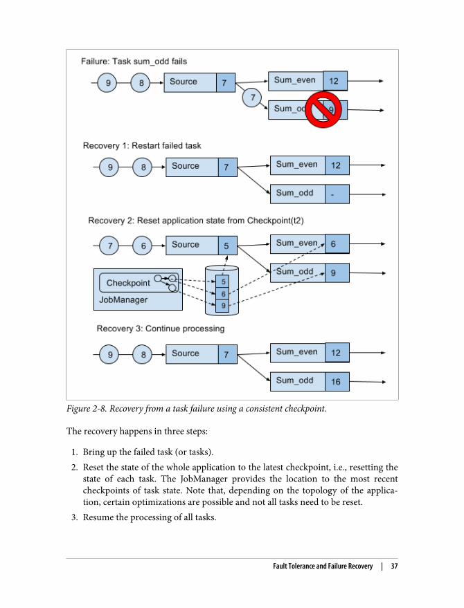
Figure 2-8. Recovery from a task failure using a consistent checkpoint.

The recovery happens in three steps:

1. Bring up the failed task (or tasks).2. Reset the state of the whole application to the latest checkpoint, i.e., resetting the

state of each task. The JobManager provides the location to the most recentcheckpoints of task state. Note that, depending on the topology of the applica‐tion, certain optimizations are possible and not all tasks need to be reset.

3. Resume the processing of all tasks.


7 Note that there are other resettable sources. In addition it is possible to implement a source function that buf‐fers records inside operator state to replay them in case of a failure.

This checkpointing and recovery mechanism is able to provide exactly-once consis‐tency for applications, given that all operators checkpoint and restore all of their stateand that all data sources of the application checkpoint their reading position in theirinput stream and are able to continue reading from a position that was reset by acheckpoint. Whether a data source is resettable or not depends on its implementationand the external system or interface from which a stream is consumed. For instance,Apache Kafka supports to read records from a previous offset of the stream. In con‐trast, a stream consumed from a socket cannot be reset because sockets do not bufferdata which has been emitted. Consequently, an application can only be operatedunder exactly-once failure semantics if it consumes all data from resettable data sour‐ces such as Flink’s connector for Apache Kafka 7

When an application is restarted from a checkpoint, its internal state is exactly thesame as when the checkpoint was taken. When it restarts, the application consumesand processes all data that was processed between the checkpoint and the failureanother time. Although this means that some messages are processed twice (beforeand after the failure) by Flink operators, the mechanism still achieves exactly-oncestate semantics because the state of all operators has been reset to a point that had notseen this data yet. We also need to point out that the checkpointing and recoverymechanism does only reset the internal state of a streaming application. Flink is ingeneral not able to invalidate records that have been sent out or to rollback changesdone to external systems. Even if the state of an application is guaranteed to haveexactly-once semantics, a data sink might emit a record more than once duringrecovery. Nonetheless, it is also possible to achieve exactly-once output semantics forselected data sinks. The challenge of end-to-end exactly-once applications is dis‐cussed in detail in Chapter X.

Taking Consistent Checkpoints without Stopping the WorldsFlink’s recovery mechanism is based on consistent application checkpoints. The naiveapproach to take a checkpoint from a streaming application, i.e, to pause, checkpoint,and resume the application, suffers from its “stop-the-world” behavior and is notapplicable for applications that have even moderate latency requirements. Instead,Flink implements an algorithm which is based on the well-known Chandy-Lamportalgorithm for distributed snapshots. The algorithm does not pause the applicationbut allows to continue processing while checkpointing the state of operators. In thefollowing we explain how this algorithm works.

At the core of Flink’s checkpointing algorithm is a special type of record which iscalled checkpoint barrier. Similar to watermarks, checkpoint barriers are injected into


the regular data stream and cannot overtake or be passed by other records. A check‐point barrier logically splits a stream into two parts and the position of the barrier inthe stream defines the extent of a checkpoint. All state modifications due to recordsthat precede a barrier are included in the checkpoint while the records following thebarrier do not modify the checkpointed state. In order to identify the checkpoint towhich a barrier belongs, each barrier carries a checkpoint ID.

We continue to explain the algorithm step-by-step using the example of a simplestreaming application. The application consists of two source tasks which both con‐sume a stream of increasing numbers. The output of the source tasks is partitionedinto substreams of even and odd numbers. Each substream is processed by a task thatkeeps the highest observed number as state and forwards all records to a statelesssink. The application is depicted in the following figure.

Figure 2-9. An example streaming application with two stateful sources, two statefultasks, and two stateless sinks.

A checkpoint is initiated by the JobManager by sending a message with a new check‐point ID to each data source task as the following figure shows.


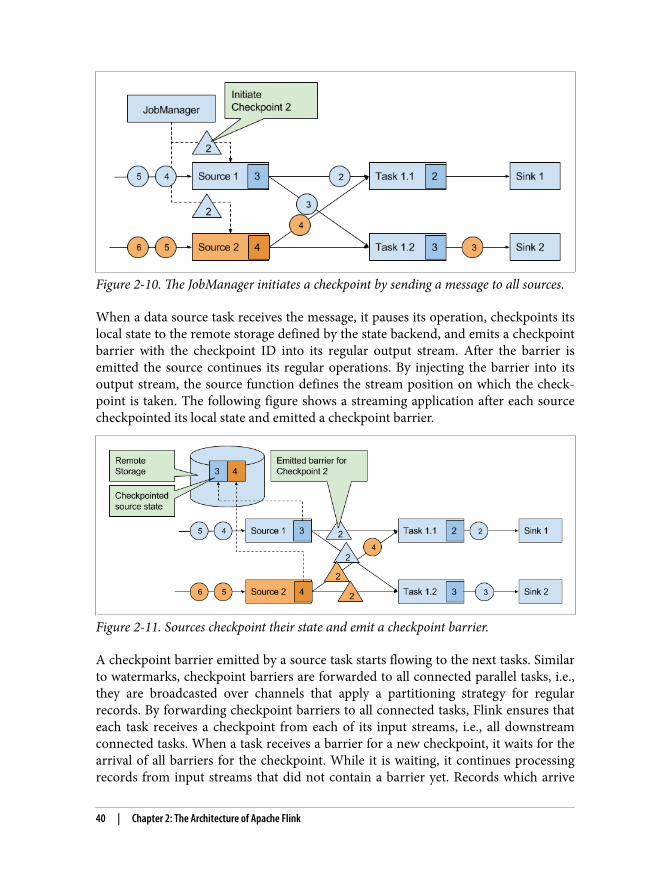
Figure 2-10. The JobManager initiates a checkpoint by sending a message to all sources.

When a data source task receives the message, it pauses its operation, checkpoints itslocal state to the remote storage defined by the state backend, and emits a checkpointbarrier with the checkpoint ID into its regular output stream. After the barrier isemitted the source continues its regular operations. By injecting the barrier into itsoutput stream, the source function defines the stream position on which the check‐point is taken. The following figure shows a streaming application after each sourcecheckpointed its local state and emitted a checkpoint barrier.

Figure 2-11. Sources checkpoint their state and emit a checkpoint barrier.

A checkpoint barrier emitted by a source task starts flowing to the next tasks. Similarto watermarks, checkpoint barriers are forwarded to all connected parallel tasks, i.e.,they are broadcasted over channels that apply a partitioning strategy for regularrecords. By forwarding checkpoint barriers to all connected tasks, Flink ensures thateach task receives a checkpoint from each of its input streams, i.e., all downstreamconnected tasks. When a task receives a barrier for a new checkpoint, it waits for thearrival of all barriers for the checkpoint. While it is waiting, it continues processingrecords from input streams that did not contain a barrier yet. Records which arrive


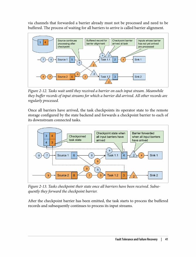
via channels that forwarded a barrier already must not be processed and need to bebuffered. The process of waiting for all barriers to arrive is called barrier alignment.

Figure 2-12. Tasks wait until they received a barrier on each input stream. Meanwhilethey buffer records of input streams for which a barrier did arrived. All other records areregularly processed.

Once all barriers have arrived, the task checkpoints its operator state to the remotestorage configured by the state backend and forwards a checkpoint barrier to each ofits downstream connected tasks.

Figure 2-13. Tasks checkpoint their state once all barriers have been received. Subse‐quently they forward the checkpoint barrier.

After the checkpoint barrier has been emitted, the task starts to process the bufferedrecords and subsequently continues to process its input streams.


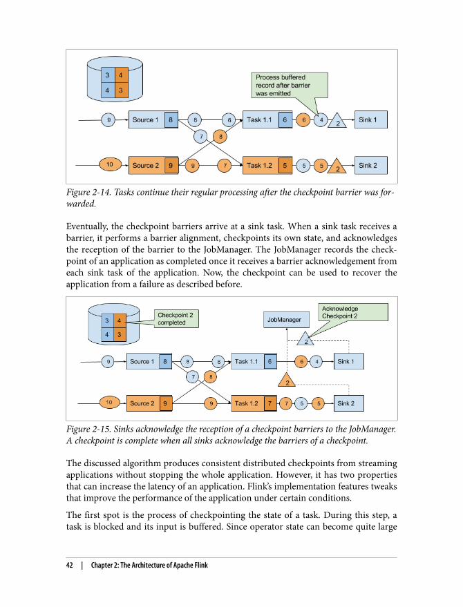
Figure 2-14. Tasks continue their regular processing after the checkpoint barrier was for‐warded.

Eventually, the checkpoint barriers arrive at a sink task. When a sink task receives abarrier, it performs a barrier alignment, checkpoints its own state, and acknowledgesthe reception of the barrier to the JobManager. The JobManager records the check‐point of an application as completed once it receives a barrier acknowledgement fromeach sink task of the application. Now, the checkpoint can be used to recover theapplication from a failure as described before.

Figure 2-15. Sinks acknowledge the reception of a checkpoint barriers to the JobManager.A checkpoint is complete when all sinks acknowledge the barriers of a checkpoint.

The discussed algorithm produces consistent distributed checkpoints from streamingapplications without stopping the whole application. However, it has two propertiesthat can increase the latency of an application. Flink’s implementation features tweaksthat improve the performance of the application under certain conditions.

The first spot is the process of checkpointing the state of a task. During this step, atask is blocked and its input is buffered. Since operator state can become quite large


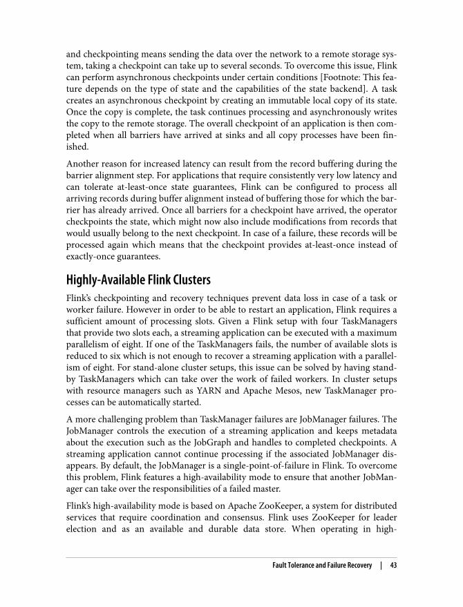
and checkpointing means sending the data over the network to a remote storage sys‐tem, taking a checkpoint can take up to several seconds. To overcome this issue, Flinkcan perform asynchronous checkpoints under certain conditions [Footnote: This fea‐ture depends on the type of state and the capabilities of the state backend]. A taskcreates an asynchronous checkpoint by creating an immutable local copy of its state.Once the copy is complete, the task continues processing and asynchronously writesthe copy to the remote storage. The overall checkpoint of an application is then com‐pleted when all barriers have arrived at sinks and all copy processes have been fin‐ished.

Another reason for increased latency can result from the record buffering during thebarrier alignment step. For applications that require consistently very low latency andcan tolerate at-least-once state guarantees, Flink can be configured to process allarriving records during buffer alignment instead of buffering those for which the bar‐rier has already arrived. Once all barriers for a checkpoint have arrived, the operatorcheckpoints the state, which might now also include modifications from records thatwould usually belong to the next checkpoint. In case of a failure, these records will beprocessed again which means that the checkpoint provides at-least-once instead ofexactly-once guarantees.

Highly-Available Flink ClustersFlink’s checkpointing and recovery techniques prevent data loss in case of a task orworker failure. However in order to be able to restart an application, Flink requires asufficient amount of processing slots. Given a Flink setup with four TaskManagersthat provide two slots each, a streaming application can be executed with a maximumparallelism of eight. If one of the TaskManagers fails, the number of available slots isreduced to six which is not enough to recover a streaming application with a parallel‐ism of eight. For stand-alone cluster setups, this issue can be solved by having stand-by TaskManagers which can take over the work of failed workers. In cluster setupswith resource managers such as YARN and Apache Mesos, new TaskManager pro‐cesses can be automatically started.

A more challenging problem than TaskManager failures are JobManager failures. TheJobManager controls the execution of a streaming application and keeps metadataabout the execution such as the JobGraph and handles to completed checkpoints. Astreaming application cannot continue processing if the associated JobManager dis‐appears. By default, the JobManager is a single-point-of-failure in Flink. To overcomethis problem, Flink features a high-availability mode to ensure that another JobMan‐ager can take over the responsibilities of a failed master.

Flink’s high-availability mode is based on Apache ZooKeeper, a system for distributedservices that require coordination and consensus. Flink uses ZooKeeper for leaderelection and as an available and durable data store. When operating in high-


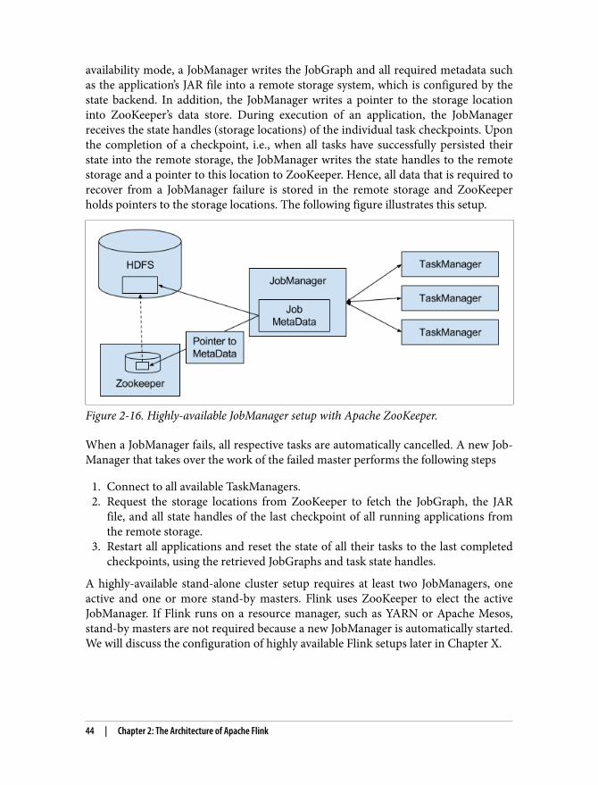
availability mode, a JobManager writes the JobGraph and all required metadata suchas the application’s JAR file into a remote storage system, which is configured by thestate backend. In addition, the JobManager writes a pointer to the storage locationinto ZooKeeper’s data store. During execution of an application, the JobManagerreceives the state handles (storage locations) of the individual task checkpoints. Uponthe completion of a checkpoint, i.e., when all tasks have successfully persisted theirstate into the remote storage, the JobManager writes the state handles to the remotestorage and a pointer to this location to ZooKeeper. Hence, all data that is required torecover from a JobManager failure is stored in the remote storage and ZooKeeperholds pointers to the storage locations. The following figure illustrates this setup.

Figure 2-16. Highly-available JobManager setup with Apache ZooKeeper.

When a JobManager fails, all respective tasks are automatically cancelled. A new Job‐Manager that takes over the work of the failed master performs the following steps

1. Connect to all available TaskManagers.2. Request the storage locations from ZooKeeper to fetch the JobGraph, the JAR

file, and all state handles of the last checkpoint of all running applications fromthe remote storage.

3. Restart all applications and reset the state of all their tasks to the last completedcheckpoints, using the retrieved JobGraphs and task state handles.

A highly-available stand-alone cluster setup requires at least two JobManagers, oneactive and one or more stand-by masters. Flink uses ZooKeeper to elect the activeJobManager. If Flink runs on a resource manager, such as YARN or Apache Mesos,stand-by masters are not required because a new JobManager is automatically started.We will discuss the configuration of highly available Flink setups later in Chapter X.


SummaryIn this chapter we have discussed Flink’s high-level architecture and the internals ofits networking stack, event-time processing mode, and failure recovery mechanism.Knowledge about these internals can be helpful when designing advanced streamingapplications, setting up and configuring clusters, and operating streaming applica‐tions as well as reasoning about their performance.

Summary | 45

lightbend fast data platform · lightbend fast data platform encapsulates the best of breed stream...

Documents