likelihood-based scoring rules for comparing density
TRANSCRIPT

HAL Id: hal-00834423https://hal.archives-ouvertes.fr/hal-00834423
Submitted on 15 Jun 2013
HAL is a multi-disciplinary open accessarchive for the deposit and dissemination of sci-entific research documents, whether they are pub-lished or not. The documents may come fromteaching and research institutions in France orabroad, or from public or private research centers.
L’archive ouverte pluridisciplinaire HAL, estdestinée au dépôt et à la diffusion de documentsscientifiques de niveau recherche, publiés ou non,émanant des établissements d’enseignement et derecherche français ou étrangers, des laboratoirespublics ou privés.
Likelihood-based scoring rules for comparing densityforecasts in tails
Cees Diks, Valentyn Panchenko, Dick van Dijk
To cite this version:Cees Diks, Valentyn Panchenko, Dick van Dijk. Likelihood-based scoring rules for comparing densityforecasts in tails. Econometrics, MDPI, 2011, 10.1016/j.jeconom.2011.04.001. hal-00834423
Accepted Manuscript
Likelihood-based scoring rules for comparing density forecasts in tails
Cees Diks, Valentyn Panchenko, Dick van Dijk
PII: S0304-4076(11)00080-7DOI: 10.1016/j.jeconom.2011.04.001Reference: ECONOM 3477
To appear in: Journal of Econometrics
Received date: 9 April 2009Revised date: 10 April 2011Accepted date: 18 April 2011
Please cite this article as: Diks, C., Panchenko, V., van Dijk, D., Likelihood-based scoringrules for comparing density forecasts in tails. Journal of Econometrics (2011),doi:10.1016/j.jeconom.2011.04.001
This is a PDF file of an unedited manuscript that has been accepted for publication. As aservice to our customers we are providing this early version of the manuscript. The manuscriptwill undergo copyediting, typesetting, and review of the resulting proof before it is published inits final form. Please note that during the production process errors may be discovered whichcould affect the content, and all legal disclaimers that apply to the journal pertain.
Likelihood-Based Scoring Rules for Comparing DensityForecasts in Tails
Cees Diks∗
Department of Quantitative EconomicsUniversity of Amsterdam
Valentyn Panchenko†
School of EconomicsUniversity of New South Wales
Dick van Dijk‡
Econometric InstituteErasmus University Rotterdam
April 7, 2011
Abstract
We propose new scoring rules based on conditional and censored likelihood for assessing the predic-tive accuracy of competing density forecasts over a specific region of interest, such as the left tail infinancial risk management. These scoring rules can be interpreted in terms of Kullback-Leibler diver-gence between weighted versions of the density forecast and the true density. Existing scoring rulesbased on weighted likelihood favor density forecasts with more probability mass in the given region,rendering predictive accuracy tests biased towards such densities. Using our novel likelihood-basedscoring rules avoids this problem.
Keywords: density forecast evaluation; scoring rules; weighted likelihood ratio scores; conditionallikelihood; censored likelihood; risk management.
JEL Classification: C12; C22; C52; C53
∗Center for Nonlinear Dynamics in Economics and Finance, Department of Quantitive Economics, University of Amster-dam, Roetersstraat 11, NL-1018 WB Amsterdam, The Netherlands. E-mail: [email protected]†School of Economics, Faculty of Business, University of New South Wales, Sydney, NSW 2052, Australia. E-mail:
[email protected]‡Econometric Institute, Erasmus University Rotterdam, P.O. Box 1738, NL-3000 DR Rotterdam, The Netherlands. E-mail:
[email protected] (corresponding author)

1 Introduction
The interest in density forecasts is rapidly expanding in both macroeconomics and finance. Undoubtedly
this is due to the increased awareness that point forecasts are not very informative unless some indication
of their uncertainty is provided, see Granger and Pesaran (2000) and Garratt et al. (2003) for discussions
of this issue. Density forecasts, representing a full predictive distribution of the random variable in ques-
tion, provide the most complete measure of this uncertainty. Prominent macroeconomic applications are
density forecasts of output growth and inflation obtained from a variety of sources, including statisti-
cal time series models (Clements and Smith, 2000), professional forecasters (Diebold et al., 1999), and
central banks and other institutions producing so-called ‘fan charts’ for these variables (Clements, 2004;
Mitchell and Hall, 2005). In finance, density forecasts play a pivotal role in risk management as they
form the basis for risk measures such as Value-at-Risk (VaR) and Expected Shortfall (ES), see Dowd
(2005) and McNeil et al. (2005) for general overviews and Guidolin and Timmermann (2006) for a
recent empirical application.1
The increasing popularity of density forecasts has naturally led to the development of statistical tools
for evaluating their accuracy. The techniques that have been proposed for this purpose can be classified
into two groups. First, several approaches have been put forward for testing the quality of an individual
density forecast, relative to the data-generating process. Following the seminal contribution of Diebold et
al. (1998), the most prominent tests in this group are based on the probability integral transform (PIT) of
Rosenblatt (1952).2 We refer to Clements (2005) and Corradi and Swanson (2006c) for in-depth surveys
on specification tests for univariate density forecasts.
The second group of evaluation tests aims to compare two or more competing density forecasts. This
problem of relative predictive accuracy has been considered by Sarno and Valente (2004), Mitchell and
Hall (2005), Corradi and Swanson (2005, 2006b), Amisano and Giacomini (2007) and Bao et al. (2004,
1In addition, density forecasts are starting to be used in other financial decision problems, such as derivative pricing(Campbell and Diebold, 2005; Taylor and Buizza, 2006; Hardle and Hlavka, 2009) and asset allocation (Guidolin and Tim-mermann, 2007). It is also becoming more common to use density forecasts to assess the adequacy of predictive regres-sion models for asset returns, including stocks (Perez-Quiros and Timmermann, 2001), interest rates (Hong et al., 2004;Egorov et al., 2006) and exchange rates (Sarno and Valente, 2005; Rapach and Wohar, 2006), as well as measures of financialmarket volatility (Bollerslev et al., 2009; Corradi et al., 2009).
2Alternative test statistics based on the PIT are developed in Berkowitz (2001), Bai (2003), Bai and Ng (2005), Hong and Li(2005), Li and Tkacz (2006), and Corradi and Swanson (2006a), mainly to counter the problems caused by parameter estimationuncertainty and the assumption of correct dynamic specification under the null hypothesis.
1

2007). All statistics in this group compare the relative distance between the competing density forecasts
and the true (but unobserved) density, albeit in different ways. Sarno and Valente (2004) consider the
integrated squared difference between the density forecast and the true density as distance measure, while
Corradi and Swanson (2005, 2006b) employ the mean squared error between the cumulative distribution
function (CDF) of the density forecast and the true CDF. The other studies in this group develop tests
of equal predictive ability based on a comparison of the Kullback-Leibler Information Criterion (KLIC).
Amisano and Giacomini (2007) provide an interesting interpretation of the KLIC-based comparison
in terms of scoring rules, which are loss functions depending on the density forecast and the actually
observed data. In particular, it is shown that the difference between the logarithmic scoring rule for two
competing density forecasts corresponds exactly to their relative KLIC values.
In many applications of density forecasts, we are mostly interested in a particular region of the
density. Financial risk management is an example in case, where the main concern is obtaining an
accurate description of the left tail of the distribution of asset returns. Bao et al. (2004) and Amisano
and Giacomini (2007) suggest likelihood ratio (LR) tests based on weighting the KLIC-type logarithmic
scoring rule for the purpose of evaluating and comparing density forecasts over a particular region.
However, as mentioned by Corradi and Swanson (2006c) the accuracy of density forecasts in a specific
region cannot be measured in a straightforward manner using the KLIC. The problem that occurs is
that by construction the weighted logarithmic scoring rule favors density forecasts with more probability
mass in the region of interest, rendering the resulting tests of equal predictive ability biased towards such
density forecasts.
In this paper we demonstrate that two density forecasts can still be compared on a specific region of
interest by means of likelihood-based scoring rules in a natural way. Our proposed solution is to replace
the full likelihood by the conditional likelihood, given that the actual observation lies in the region of
interest, or by the censored likelihood, with censoring of the observations outside the region of inter-
est. We show analytically that these new scoring rules can be interpreted in terms of Kullback-Leibler
divergences between weighted versions of the density forecast and the actual density. This implies that
the conditional likelihood and censored likelihood scoring rules favor density forecasts that approximate
the true conditional density as closely as possible in the region of interest. Consequently, tests of equal
2
predictive accuracy of density forecasts based on these scoring rules do not suffer from spurious rejec-
tions against densities with more probability mass in that region. This is confirmed by extensive Monte
Carlo simulations, in which we assess the finite sample properties of the predictive ability tests for the
different scoring rules. Here we also find that the censored likelihood scoring rule, which uses more of
the relevant information present, performs better in most, but not all, cases considered.
We wish to emphasize that the framework developed here differs from the evaluation of conditional
quantile forecasts as considered in Giacomini and Komunjer (2005). That approach focuses on the
predictive accuracy of point forecasts for a specific quantile of interest, such as the VaR at a certain level,
whereas the conditional and censored likelihood scoring rules intend to cover a broader region of the
density. We do not claim that our methodology is a substitute for the quantile forecast evaluation test (or
any other predictive accuracy test), but suggest that they may be used in a complementary way.
Gneiting and Ranjan (2008) independently also address the tendency of the weighted LR test of
Amisano and Giacomini (2007) to favor density forecasts with more probability mass in the region of
interest, but from a quantile forecast evaluation perspective. They point out that this tendency is a con-
sequence of the scoring rule not being proper (Winkler and Murphy, 1968; Gneiting and Raftery, 2007),
meaning that an incorrect density forecast may receive a higher average score than the true conditional
density. Exactly this gives rise to the problem of spuriously favoring densities with more probability mass
in the region of interest. As an alternative Gneiting and Ranjan (2008)propose weighted quantile scoring
rules. Our aim in this paper is different in that we specifically want to find alternative scoring rules that
generalize the unweighted likelihood scoring rule. The two main reasons for pursuing this are, first, that
likelihood-based score differences are invariant under transformations of the outcome space and, second,
that they lead to LR statistics, which are known to have optimal power properties, as emphasized by
Berkowitz (2001) in the context of density forecast evaluation.
The remainder of this paper is organized as follows. In Section 2, we discuss conventional scoring
rules based on the KLIC divergence for evaluating density forecasts and illustrate the problem with the
resulting LR tests in case the logarithmic scores are weighted to focus on a particular region of interest. In
Section 3 we put forward our alternative scoring rules based on conditional and censored likelihood and
show analytically that the new scoring rules are proper. We assess the finite sample properties of tests of
3

equal predictive accuracy of density forecasts based on the different scoring rules by means of extensive
Monte Carlo simulation experiments in Section 4. We provide an empirical application concerning
density forecasts for daily S&P 500 returns in Section 5, demonstrating the practical usefulness of the
new scores. We summarize and conclude in Section 6.
2 Scoring rules for evaluating density forecasts
We consider a stochastic process Zt : Ω → Rk+1Tt=1, defined on a complete probability space
(Ω,F ,P), and identify Zt with (Yt, X ′t)′, where Yt : Ω → R is the real valued random variable of
interest and Xt : Ω → Rk is a vector of observable predictor variables. The information set at time t
is defined as Ft = σ(Z ′1, . . . , Z ′t)′. We consider the case where two competing forecast methods are
available, each producing one-step ahead density forecasts, i.e. predictive densities of Yt+1, based on Ft.
The competing density forecasts of Yt+1 are denoted by the probability density functions (pdfs) ft(y)
and gt(y), respectively. As in Amisano and Giacomini (2007), by ‘forecast method’ we mean the set
of choices that the forecaster makes at the time of the prediction, including the variables Xt, the econo-
metric model (if any), and the estimation method. The only requirement that we impose on the forecast
methods is that the density forecasts depend only on a finite number m of most recent observations
Zt−m+1, . . . , Zt. Forecast methods of this type arise naturally, for instance, when density forecasts are
obtained from time series regression models, for which parameters are estimated with a moving window
ofm observations. The reason for focusing on forecast methods rather than on forecast models is that this
allows for treating parameter estimation uncertainty as an integral part of the density forecasts. Requiring
the use of a finite (rolling) window of m past observations for parameter estimation then considerably
simplifies the asymptotic theory of tests of equal predictive accuracy, as demonstrated by Giacomini and
White (2006). It also turns out to be convenient as it enables comparison of density forecasts based on
both nested and non-nested models, in contrast to other approaches such as West (1996).
Our interest lies in comparing the relative performance of the one-step-ahead density forecasts ft(y)
and gt(y). One of the approaches that has been put forward for this purpose is based on scoring rules,
which are commonly used in probability forecast evaluation, see Diebold and Lopez (1996). In the
current context, a scoring rule is a loss function S∗(ft; yt+1) depending on the density forecast and the
4

actually observed value yt+1, such that a density forecast that is ‘better’ receives a higher score. Of
course, what is considered to be a better forecast among two competing incorrect forecasts depends on
the measure used to quantify divergences between distributions. However, as argued by Diebold et al.
(1998) and Granger and Pesaran (2000), any rational user would prefer the true conditional density pt of
Yt+1 over an incorrect density forecast. This suggests that it is natural to focus, if possible, on scoring
rules that are such that incorrect density forecasts ft do not receive a higher average score than the true
conditional density, that is,
Et(S(ft;Yt+1)
)≤ Et (S(pt;Yt+1)) , for all t.
Following Gneiting and Raftery (2007), a scoring rule satisfying this condition will be called proper.
It is useful to note that the correct density pt includes true parameters (if any). In practice, den-
sity forecasts typically involve estimated parameters. This implies that even if the density forecast ft
is based on a correctly specified model, but the model includes estimated parameters, the average score
Et(S(ft;Yt+1)
)may not achieve the upper bound Et (S(pt;Yt+1)) due to nonvanishing estimation un-
certainty. This reflects the fact that a density forecast based on a misspecified model with limited es-
timation uncertainty may be preferred over a density forecast based on the correct model specification
having larger estimation uncertainty. Section 4.3 illustrates this issue with a Monte Carlo simulation.
The above may seem to suggest that the notion of properness of scoring rules is of limited relevance
in practice. Nevertheless, it does appear to be a desirable characteristic. Proper scoring rules are such
that density forecasts receive a higher score when they approximate the true conditional density more
closely, for example in the Kullback-Leibler sense as with the logarithmic score (2) discussed below. We
have to keep in mind though that in the presence of nonvanishing estimation uncertainty, as accounted
for in the adopted framework of Giacomini and White (2006), this may be a density forecast based on a
misspecified model.
Given a scoring rule of one’s choice, there are various ways to construct tests of equal predictive
ability. Giacomini and White (2006) distinguish tests for unconditional predictive ability and conditional
predictive ability. In the present paper, for clarity of exposition, we focus on tests for unconditional
5
predictive ability.3 Assume that two competing density forecasts ft and gt and corresponding realizations
of the variable Yt+1 are available for t = m,m + 1, . . . , T − 1. We may then compare ft and gt based
on their average scores, by testing formally whether their difference is statistically significant. Defining
the score difference
d∗t+1 = S∗(ft; yt+1)− S∗(gt; yt+1),
for a given scoring rule S∗, the null hypothesis of equal scores is given by
H0 : E(d∗t+1) = 0, for all t = m,m+ 1, . . . , T − 1.
Let d∗m,n denote the sample average of the score differences, that is, d
∗m,n = n−1
∑T−1t=m d
∗t+1 with
n = T −m. In order to test H0 against the alternative Ha: E(d∗m,n
)6= 0, (or < 0 or > 0) we may use
a Diebold and Mariano (1995) type statistic
tm,n =d∗m,n√σ2m,n/n
, (1)
where σ2m,n is a heteroskedasticity and autocorrelation-consistent (HAC) variance estimator of σ2
m,n =
Var(√
nd∗m,n
), which satisfies σ2
m,n−σ2m,n
P−→ 0. The following theorem characterizes the asymptotic
distribution of the test statistic under the null hypothesis.
Theorem 1 The statistic tm,n in (1) is asymptotically (as n → ∞ with m fixed) standard normally
distributed under the null hypothesis if: (i) Zt is φ-mixing of size −q/(2q − 2) with q ≥ 2, or α-
mixing of size−q/(q−2) with q > 2; (ii) E|d∗t+1|2q <∞ for all t; and (iii) σ2m,n = Var
(√nd∗m,n
)> 0
for all n sufficiently large.
Proof: This is Theorem 4 of Giacomini and White (2006), where a proof can also be found. 2
The proof of this theorem as given by Giacomini and White (2006) is based on the central limit
theorems for dependent heterogeneous processes given in Wooldridge and White (1988). The conditions
in Theorem 1 are rather weak in that they allow for nonstationarity and heterogeneity. However, note
that conditions (i) and (ii) jointly imply the existence of at least the fourth moment of d∗t+1 for all t.
3The above inequality in terms of conditional expectations implies the same inequality in terms of unconditional expecta-
tions, that is, E“Et
“S(ft;Yt+1)
””≤ E (Et (S(pt;Yt+1)))⇒ E
“S(ft;Yt+1)
”≤ E (S(pt;Yt+1))
6

Theorem 1.3 of Merlevede and Peligrad (2000) shows that asymptotic normality can also be achieved
under weaker distributional assumptions (existence of the second moment plus a condition relating the
behavior of the tail of the distribution of |d∗t+1| to the mixing rate). However, strict stationarity is assumed
by Merlevede and Peligrad (2000). The conditions required for asymptotic normality of normalized
partial sums of dependent heterogeneous random variables have been further explored by De Jong (1997).
2.1 The logarithmic scoring rule and the Kullback-Leibler information criterion
Mitchell and Hall (2005), Amisano and Giacomini (2007), and Bao et al. (2004, 2007) focus on the
logarithmic scoring rule
Sl(ft; yt+1) = log ft(yt+1), (2)
assigning a high score to a density forecast if the observation yt+1 falls within a region with high pre-
dictive density ft, and a low score if it falls within a region with low predictive density. Based on the
n observations available for evaluation, ym+1, . . . , yT , the density forecasts ft and gt can be ranked
according to their average scores n−1∑T−1
t=m log ft(yt+1) and n−1∑T−1
t=m log gt(yt+1). The density fore-
cast yielding the highest average score would obviously be the preferred one. The sample average of
the log score differences dlt+1 = log ft(yt+1) − log gt(yt+1) may be used to test whether the predictive
accuracy is significantly different, using the test statistic defined in (1). Note that this coincides with the
log-likelihood ratio of the two competing density forecasts.
Intuitively, the logarithmic scoring rule is closely related to information theoretic goodness-of-fit
measures such as the Kullback-Leibler Information Criterion (KLIC), which for the density forecast ft
is defined as
KLIC(ft) = Et(
log pt(Yt+1)− log ft(Yt+1))
=∫ ∞−∞
pt(yt+1) log
(pt(yt+1)
ft(yt+1)
)dyt+1, (3)
where pt denotes the true conditional density. Obviously, a higher expected value (with respect to the
true density pt) of the logarithmic score in (2) is equivalent to a lower value of the KLIC in (3). Under
the constraint∫∞−∞ ft(y) dy = 1, the expectation of log ft(Yt+1) with respect to the true density pt is
maximized by taking ft = pt. This follows from the fact that for any density ft different from pt,
Et
(log
(ft(Yt+1)pt(Yt+1)
))≤ Et
(ft(Yt+1)pt(Yt+1)
)− 1 =
∫ ∞−∞
pt(y)ft(y)pt(y)
dy − 1 = 0,
7

where the inequality follows from applying log x ≤ x− 1 to ft/pt.
It thus follows that the quality of a normalized density forecast ft can be measured properly by the
log-likelihood score Sl(ft; yt+1) and, equivalently, by the KLIC in (3). An advantage of the KLIC is that
it has an absolute lower bound equal to zero, which is achieved if and only if the density forecast ft is
identical to the true distribution pt. As such, its value provides a measure of the divergence between the
candidate density ft and pt. However, since pt is unknown, the KLIC cannot be evaluated directly (but
we return to this point below). We can nevertheless use the KLIC to measure the relative accuracy of
two competing densities, as discussed in Mitchell and Hall (2005) and Bao et al. (2004, 2007). Taking
the difference KLIC(gt) − KLIC(ft) the term Et (log pt(Yt+1)) drops out, solving the problem that the
true density pt is unknown. This in fact renders the logarithmic score difference dlt+1 = log ft(yt+1) −
log gt(yt+1).
Summarizing the above, the null hypothesis of equal average logarithmic scores for the density fore-
casts ft and gt actually corresponds with the null hypothesis of equal KLICs. Given that the KLIC
measures the divergence of the density forecasts from the true density, the use of the logarithmic scoring
rule boils down to assessing which of the competing densities comes closest to the true distribution.
Bao et al. (2004, 2007) discuss an extension to compare multiple density forecasts based on their
KLIC values, where the null hypothesis is that none of the available density forecasts is more accurate
than a given benchmark, in the spirit of the reality check of White (2000). Mitchell and Hall (2005) and
Hall and Mitchell (2007) also use the relative KLIC values as a basis for combining density forecasts.
It is useful to note that both Mitchell and Hall (2005) and Bao et al. (2004, 2007) employ the KLIC
for testing the null hypothesis of an individual density forecast being correct, that is, H0 : KLIC(ft) =
0. The problem that the true density pt in (3) is unknown then is circumvented by using the result
established by Berkowitz (2001) that the KLIC of the density forecast ft relative to pt is equal to the
KLIC of the density of the inverse normal transform of the PIT of ft relative to the standard normal
density. Defining zf ,t+1 = Φ−1(Ft(yt+1)) with Ft(yt+1) =∫ yt+1
−∞ ft(y) dy and Φ the standard normal
distribution function, it holds true that
log pt(yt+1)− log ft(yt+1) = log qt(zf ,t+1)− log φ(zf ,t+1),
8

where qt is the true conditional density of zf ,t+1 and φ is the standard normal density. This result states
that the logarithmic scores are invariant to the inverse normal transform of yt+1, which is essentially a
consequence of the general invariance of likelihood ratios under smooth coordinate transformations. Of
course, in practice the density qt is not known either, but it may be estimated using a flexible density
function. The resulting KLIC estimate then allows testing for departures of qt from the standard normal.
2.2 Weighted logarithmic scoring rules
In empirical applications of density forecasting it frequently occurs that a particular region of the density
is of most interest. For example, in risk management applications such as VaR and ES estimation, an
accurate description of the left tail of the distribution of asset returns obviously is of crucial importance.
In that context, it seems natural to focus on the performance of density forecasts in the region of interest
and pay less attention to (or even ignore) the remaining part of the distribution.
Within the framework of scoring rules, an obvious way to pursue this is to construct a weighted
scoring rule, using a weight function wt(y) to emphasize the region of interest (see Franses and van Dijk
(2003) for a similar idea in the context of testing equal predictive accuracy of point forecasts). Along
this line Amisano and Giacomini (2007) propose the weighted logarithmic (wl) scoring rule
Swl(ft; yt+1) = wt(yt+1) log ft(yt+1) (4)
to assess the quality of density forecast ft on a certain region defined by the properties of wt(yt+1). The
weighted average scores n−1∑T−1
t=mwt(yt+1) log ft(yt+1) and n−1∑T−1
t=mwt(yt+1) log gt(yt+1) can be
used for ranking two competing forecasts, while the weighted score difference
dwlt+1 = Swl(ft; yt+1)− Swl(gt; yt+1) = wt(yt+1)(log ft(yt+1)− log gt(yt+1)), (5)
forms the basis for testing the null hypothesis of equal weighted scores, H0 : E(dwlt+1
)= 0, for all
t = m,m+ 1, . . . , T , by means of a Diebold-Mariano type statistic of the form (1).
For the sake of argument it is instructive to consider the case of a ‘threshold’ weight function
wt(y) = I(y ≤ r), with a fixed threshold r, where I(A) = 1 if the event A occurs and zero other-
wise. This is a simple example of a weight function we might consider for evaluation of the left tail in
risk management applications. In this case, however, the weighted logarithmic score results in predictive
9

ability tests that are biased towards densities with more probability mass in the left tail. This can be
seen by considering the situation where gt(y) > ft(y) for all y smaller than some given value y∗, say.
Using wt(y) = I(y ≤ r) for some r < y∗ in (4) implies that the weighted score difference dwlt+1 in (5)
is never positive, and strictly negative for observations below the threshold value r, such that E(dwlt+1)
is negative. Obviously, this can have far-reaching consequences when comparing density forecasts with
different tail behavior. In particular, it may happen that a (relatively) fat-tailed distribution gt is favored
over a thin-tailed distribution ft, even if the latter is the true distribution from which the data are drawn,
as the following example illustrates.
Figure 1 about here
Example 1 Suppose we wish to compare the accuracy of two density forecasts for Yt+1, one being the
standard normal distribution with pdf
ft(y) = (2π)−12 exp(−y2/2),
and the other being the Student-t distribution with ν degrees of freedom, standardized to unit variance,
with pdf
gt(y) =Γ(ν+12
)√(ν − 2)πΓ(ν2 )
(1 +
y2
(ν − 2)
)−(ν+1)/2
, with ν > 2.
Figure 1 shows these density functions for the case ν = 5, as well as the relative log-likelihood score
log ft(yt+1) − log gt(yt+1). The relative score function is negative in the left tail (−∞, y∗), with
y∗ ≈ −2.5. Now consider the situation that we have a sample ym+1, . . . , yT of n observations from
an unknown density on (−∞,∞) for which ft(y) and gt(y) are competing candidates, and we use a
threshold weight function wt(y) = I(y ≤ r), with fixed threshold r, to concentrate on the left tail. It
follows from the lower panel of Figure 1 that if the threshold r < y∗, the average weighted log-likelihood
score difference dwlm,n can never be positive and will be strictly negative whenever there are observations
in the tail. Evidently, the test of equal predictive accuracy will then favor the fat-tailed Student-t density
gt(y), even if the true density is the standard normal ft(y). 2
10
2.3 Weighted probability scores
The issue we are signalling has been reported independently by Gneiting and Ranjan (2008). As they
point out, the wl score does not satisfy the properness property, in the sense that there can be incorrect
density forecasts ft that receive a higher average score than the actual conditional density pt. As a
consequence, the associated test of equal predictive accuracy could even suggest that the incorrect density
forecast is significantly better than the true density.
As discussed before, it seems reasonable to focus on proper scoring rules to avoid such inconsisten-
cies. However, there are many different proper scoring rules one might use, raising the question which
rules are suitable candidates in practice. Our main reason to focus on KLIC-based scoring rules is the
close connection with likelihood ratio tests, which are known to perform well in many statistical settings.
As mentioned before, the test for equal predictive ability based on the logarithmic scoring rule is nothing
but a likelihood ratio test.
Before introducing our proper likelihood-based scoring rules, we briefly summarize the scoring rules
proposed by Gneiting and Ranjan (2008), which may also be used for comparing density forecasts in
specific regions of interest. Their starting point is the continuous ranked probability score (CRPS),
which for the density forecast ft is defined as
CRPS(ft, yt+1) =∫ ∞−∞
PS(Ft(r), I(yt+1 ≤ r)) dr, (6)
where
PS(Ft(r), I(yt+1 ≤ r)) = (I(yt+1 ≤ r)− Ft(r))2
is the Brier probability score for the probability forecast Ft(r) =∫ r−∞ ft(y)dy of the event Yt+1 ≤ r.
Equivalently, the CRPS may be written in terms of α-quantile forecasts qt,α = F−1t (α), as
CRPS(ft, yt+1) =∫ 1
0QSα(qt,α, yt+1) dα, (7)
where
QSα(qt,α, yt+1) = 2(α− I(yt+1 < qt,α))(yt+1 − qt,α)
is the quantile score (also known as the ‘tick’ or ‘check’ score) function, see also Giacomini and Ko-
munjer (2005). As suggested by Gneiting and Ranjan (2008), the CRPS in (7) may be generalized to
11

emphasize certain regions of interest in the evaluation of density forecasts. Specifically, a weighted
quantile scoring rule (wqs) may be defined as
Swqs(ft; yt+1) = −∫ 1
0v(α)QSα(qt,α, yt+1) dα,
where v(α) is a nonnegative weight function on the unit interval and the minus sign on the right-hand side
is inserted such that density forecasts with higher scores are preferred. Similarly, a weighted probability
score (wps) is obtained from (6) as
Swps(ft; yt+1) = −∫ ∞−∞
wt(r)PS(Ft(r), I(yt+1 ≤ r)) dr, (8)
for some weight function wt. Note that the same wps scoring rule was proposed by Corradi and Swanson
(2006b) for evaluating density forecasts in case a specific region of the density is of interest rather than
its whole support. In the Monte Carlo simulations in Section 4, we include Diebold-Mariano type tests
based on Swps(ft; yt+1) for comparison purposes.
3 Scoring rules based on conditional and censored likelihood
KLIC-based scoring rules for evaluating and comparing density forecasts in a specific region of interest
At ⊂ R can be obtained in a relatively straightforward manner. Specifically, it is natural to replace the
full likelihood in (2) either by the conditional likelihood, given that the observation lies in the region of
interest, or by the censored likelihood.
The conditional likelihood (cl) score function, given a region of interest At, is given by
Scl(ft; yt+1) = I(yt+1 ∈ At) log
(ft(yt+1)∫Atft(s)ds
). (9)
The main argument for using this scoring rule would be to evaluate density forecasts based only on their
behavior in the region of interest At. The division by∫Atft(s)ds serves the purpose of normalizing the
density on the region of interest, such that competing density forecasts can be compared in terms of their
relative KLIC-values, as discussed before.
However, due to this normalization, the cl scoring rule does not take into account the accuracy of
the density forecast for the total probability of the region of interest. For example, in case At is the
left tail yt+1 ≤ r, the conditional likelihood ignores whether the tail probability implied by ft matches
12

with the frequency at which tail observations actually occur. As a result, the scoring rule in (9) attaches
comparable scores to density forecasts that have similar tail shapes but may have completely different
tail probabilities. This tail probability is obviously relevant for risk management purposes, in particular
for VaR evaluation, and therefore it would be useful to include it in the density forecast evaluation. This
can be achieved by using the censored likelihood (csl) score function, given by
Scsl(ft; yt+1) = I(yt+1 ∈ At) log ft(yt+1) + I(yt+1 ∈ Act) log
(∫Act
ft(s)ds
), (10)
where Act is the complement of At. This scoring rule uses the likelihood associated with having an
observation outside the region of interest, but apart from that ignores the shape of ft outside At. In that
sense this scoring rule is similar to the log-likelihood used in the Tobit model for random variables that
cannot be observed above a certain threshold value (see Tobin, 1958).
The conditional and censored likelihood scoring rules as discussed above focus on a sharply defined
region of interest At. It is possible to adapt these score functions in order to emphasize certain parts of
the outcome space more generally, by going back to the original idea of using a weight function wt(y)
as in (4). For this purpose, note that by setting wt(y) = I(y ∈ At) the scoring rules in (9) and (10) can
be rewritten as
Scl(ft; yt+1) = wt(yt+1) log
(ft(yt+1)∫wt(s)ft(s)ds
), (11)
and
Scsl(ft; yt+1) = wt(yt+1) log ft(yt+1) + (1− wt(yt+1)) log(
1−∫wt(s)ft(s)ds
). (12)
At this point, we make the following assumptions.
Assumption 1 The density forecasts ft and gt satisfy KLIC(ft) < ∞ and KLIC(gt) < ∞, where
KLIC(ht) =∫pt(y) log (pt(y)/ht(y)) dy is the Kullback-Leibler divergence between the density fore-
cast ht and the true conditional density pt.
Assumption 2 The weight function wt(y) is such that (a) it is determined by the information available
at time t, and hence a function of Ft, (b) 0 ≤ wt(y) ≤ 1, and (c)∫wt(y)pt(y) dy > 0.
Assumption 1 ensures that the expected score differences for the competing density forecasts are finite.
13

Assumption 2 (c) is needed to avoid cases where wt(y) takes strictly positive values only outside the
support of the data.
The following lemma shows that the generalized cl and csl scoring rules in (11) and (12) are proper,
and hence cannot lead to spurious rejections against wrong alternatives just because these have more
probability mass in the region(s) of interest.
Lemma 1 Under Assumptions 1 and 2, the generalized conditional likelihood scoring rule given in (11)
and the generalized censored likelihood scoring rule given in (12) are proper.
The proof of this Lemma is given in Appendix A. The proof clarifies that the scoring rules in (11)
and (12) can be interpreted in terms of Kullback-Leibler divergences between weighted versions of the
density forecast and the actual density.
We may test the null hypothesis of equal performance of two density forecasts ft(yt+1) and gt(yt+1)
based on the conditional likelihood score (11) or the censored likelihood score (12) in the same manner
as before. That is, given a sample of density forecasts and corresponding realizations for n time periods
t = m,m + 1, . . . , T − 1, we may form the relative scores dclt+1 = Scl(ft; yt+1) − Scl(gt; yt+1) and
dcslt+1 = Scsl(ft; yt+1)− Scsl(gt; yt+1) and use these for computing Diebold-Mariano type test statistics
as given in (1).
Figure 2 about here
Example 1 (continued) We revisit the example from the previous section in order to illustrate the
properties of the various scoring rules and the associated tests for comparing the accuracy of competing
density forecasts. We generate 10, 000 series of n = 2, 000 independent observations yt+1 from a
standard normal distribution. For each sequence we compute the weighted logarithmic scores in (4), the
conditional likelihood scores in (11), and the censored likelihood scores in (12). We use the threshold
weight function wt(y) = I(y ≤ r), with the threshold fixed at r = −2.5. The scores are computed for
the (correct) standard normal density ft and for the standardized Student-t density gt with five degrees
of freedom. Figure 2 shows the empirical CDF of the mean relative scores d∗m,n, where ∗ is wl, cl or
csl. The average wl scores take almost exclusively negative values, which means that, on average, they
14

attach a lower score to the correct normal distribution than to the Student-t distribution, cf. Figure 1,
indicating a bias in the corresponding test statistic towards the incorrect, fat-tailed distribution. The cl
and csl scoring rules both correctly favor the true normal density. The censored likelihood rule appears to
be better at detecting the inadequacy of the Student-t distribution, in that its relative scores stochastically
dominate those based on the conditional likelihood.
To illustrate the behavior of the scoring rules obtained under smooth weight functions we consider
the logistic weight function
wt(y) = 1/(1 + exp(a(y − r))) with a > 0. (13)
This sigmoidal function changes monotonically from 1 to 0 as Yt+1 increases, while wt(r) = 12 and the
slope parameter a determines the speed of the transition. In the limit as a → ∞, the threshold weight
function I(y ≤ r) is recovered. We fix the center at r = −2.5 and vary the slope parameter a among
the values 3, 4, 6, and 10. For a = 10, the logistic weight function is already very close to the threshold
weight function I(y ≤ r), such that for larger values of a the score distributions essentially do not change
anymore. The integrals∫wt(y)ft(y) dy and
∫wt(y)gt(y) dy are determined numerically by averaging
over a large number (106) of simulated random variables Yt+1 with density ft and gt, respectively.
Figure 3 about here
Figure 3 shows the empirical CDFs of the mean relative scores d∗m,n obtained with the conditional
likelihood and censored likelihood scoring rules for the different values of a. It can be observed that the
difference between the scores increases as a becomes larger. In fact, for the smoothest weight function
considered (a = 1) the two score distributions are very similar. The cl and csl score distributions become
more alike for smaller values of a because, as a→ 0, wt(y) in (13) converges to a constant equal to 12 for
all values of y, so thatwt(y)−(1−wt(y))→ 0, and moreover∫wt(y)ft(y) dy =
∫wt(y)gt(y) dy → 1
2 .
Consequently, both scoring rules converge to the unconditional likelihood (up to a constant factor 2) and
the relative scores dclt+1 and dcslt+1 have the limit
12
(log ft(yt+1)− log gt(yt+1)).
2
15

We close this section with some remarks on the weight function wt(y) defining the region that is
emphasized in the density forecast evaluation. The conditional and censored likelihood scoring rules may
be applied with arbitrary weight functions, subject to the conditions stated in Lemma 1. The appropriate
choice ofwt(y) obviously depends on the interests of the forecast user. The threshold (or logistic) weight
function considered in the example above seems a natural choice in risk management applications, as the
left tail behavior of the density forecast is of most concern there. In other applications however the focus
may be on different regions. For example, for monetary policymakers aiming to keep inflation within a
certain range, the central part of the density may be of most interest, suggesting a weight function such
as wt(y) = I(rl ≤ y ≤ ru), for certain lower and upper bounds rl and ru.
The preceding implies that essentially it is also up to the forecast user to set the parameter(s) in
the weight function, such as the threshold r in wt(y) = I(y ≤ r). For example, when Yt represents
the return on a given portfolio, r may be set equal to a certain quantile of the return distribution such
that it corresponds with a target VaR level. In practice, r will then have to be estimated from historical
data and might be set equal to the particular quantile of the m observations in the moving window that
is used for constructing the density forecast at time t. This makes the weight function dynamic, i.e.
wt(y) = I(y ≤ rt), while it also involves estimation uncertainty, namely in the threshold rt. As shown
by Lemma 1, as long as the weight function wt is conditionally (given Ft) independent of Yt+1, the
properness property of the conditional and censored likelihood scoring rules is not affected. However,
nonvanishing estimation uncertainty in the threshold may affect the power of the test of equal predictive
accuracy. In Section 4.3, we verify this numerically with Monte Carlo simulations.
4 Monte Carlo simulations
In this section we examine the implications of using the weighted logarithmic scoring rule in (4), the
conditional likelihood score in (11), the censored likelihood score in (12), and the weighted probability
score in (8) for constructing a test of equal predictive ability of two competing density forecasts in finite
samples. Specifically, we consider the size and power properties of the Diebold-Mariano type statistic as
given in (1) for testing the null hypothesis that the two competing density forecasts have equal expected
16

scores, or
H0 : E(d∗t+1
)= 0, for t = m,m+ 1, . . . , T − 1
under scoring rule ∗, where ∗ is either wl, wps, cl or csl. As before m denotes the length of the rolling
window used for constructing the density forecast and n = T − m denotes the number of forecasts.
Throughout we use a HAC-estimator for the asymptotic variance of the average relative score d∗m,n, that
is σ2m,n = γ0 +2
∑K−1k=1 akγk, where γk denotes the lag-k sample covariance of the sequence d∗t+1T−1
t=m
and ak are the Bartlett weights ak = 1− k/K with K = bn1/4c. We focus on one-sided rejection rates
to highlight the fact that some of the scoring rules may favor a wrong density forecast over a correct one.
Concerning the implementation of the wps rule in (8), it is useful to note that it is in fact not essential
for the properness of this score function to use an integral. As mentioned by Gneiting and Ranjan
(2008), a weighted sum over a finite number of y-values also renders a suitable scoring rule. With this
in mind, we do not attempt to obtain an accurate numerical approximation to the integral in (8), which
is computationally very demanding, but simply use a discretized version with a discretization step of the
y-variable of 0.1.
Initially, we examine the size and power properties of the test of equal predictive ability in an envi-
ronment that does not involve parameter estimation uncertainty in Sections 4.1 and 4.2, to demonstrate
the pitfalls when using wl scoring rule and the benefits of the cl and csl alternatives most clearly. The
role of estimation uncertainty, both in the density forecasts and in the weighting function, are addressed
explicitly in Section 4.3.
4.1 Size
In order to assess the size properties of the tests a case is required with two competing predictive densities
that are both ‘equally (in)correct’. However, whether or not the null hypothesis of equal predictive
ability holds depends on the weight function wt(y) that is used in the scoring rules. This complicates the
simulation design, given the fact that we would like to examine how the behavior of the tests depends
on the specific settings of the weight function. For the threshold weight function wt(y) = I(y ≤ r) it
appears to be impossible to construct an example with two different density forecasts having identical
predictive ability regardless of the value of r. We therefore evaluate the size of the tests when focusing
17

on the central part of the distribution by means of the weight function wt(y) = I(−r ≤ y ≤ r). As
mentioned before, in some cases this region of the distribution may be of primary interest, for instance
to monetary policymakers targeting to keep inflation between certain lower and upper bounds. The data
generating process (DGP) is taken to be i.i.d. standard normal, while the two competing density forecasts
are normal distributions with different means equal to −0.2 and 0.2 and identical variance equal to 1. In
this case, independent of the value of r the competing density forecasts have equal predictive accuracy, as
the scoring rules considered here are invariant under a simultaneous reflection about zero of all densities
of interest (the true conditional density as well as the density forecasts). In addition, it turns out that
for this combination of DGP and predictive densities, the relative scores d∗t+1 for the wl, cl and csl rules
based on wt(y) = I(−r ≤ y ≤ r) are identical; observations outside the interval [−r, r] do not support
evidence in favor of either density forecast, which is reflected in equal scores for the two forecasts, under
any of the scoring rules considered.
Figure 4 about here
Figure 4 displays one-sided rejection rates at nominal significance levels of 1, 5 and 10% of the null
hypothesis against the alternative that theN(0.2, 1) distribution has better predictive ability as a function
of the threshold value r, based on 10, 000 replications for sample size n = 500. The rejection rates of the
tests are quite close to the nominal significance levels for all values of r. Unreported results for different
values of n show that this holds even for sample sizes as small as n = 100 observations. Hence, the size
properties of the predictive ability test appear to be satisfactory.
4.2 Power
We evaluate the power of the test based on the various scoring rules by performing simulation experi-
ments where one of the competing density forecasts is correct, i.e. corresponds exactly with the underly-
ing DGP. In that case the true density always is the best possible one, regardless of the region for which
the densities are evaluated, that is, regardless of the weight function used in the scoring rules. Given that
our main focus in this paper has been on comparing density forecasts in the left tail, in these experiments
we first return to the threshold weight function wt(y) = I(y ≤ r).
18

In order to make the rejection frequencies of the null obtained for different values of r more com-
parable, we make the sample size n dependent on the threshold value in such a way that the expected
number of observations in the region of interest, denoted by c, is constant across the various values of r.
This is achieved by setting n = c/P(Y < r). Given that in typical risk management applications there
may be only a few tail observations, we consider relatively small values of c.
Figure 5 about here
Figure 6 about here
Figures 5 and 6 show the observed rejection rates for c = 5 and c = 40, respectively, based on
10, 000 replications, for data drawn from the standard normal distribution (left column) or the standard-
ized Student-t(5) distribution (right column). In both cases, the null hypothesis being tested is equal
predictive accuracy of the standard normal and standardized Student-t(5) density forecasts. The top
(bottom) panels in these Figures show rejection rates at nominal significance level 5% against superior
predictive ability of the standard normal (standardized Student-t(5)) distribution, as a function of the
threshold parameter r. Hence, the top left and bottom right panels report true power (rejections in favor
of the correct density), while the top right and bottom left panels report spurious power (rejections in
favor of the incorrect density).
Figure 7 about here
Several interesting conclusions emerge from these graphs. First, the power of the wl scoring rule
depends strongly on the threshold parameter r. For the normal DGP, for example, the test has excellent
power for values of r between−2 and 0, but for more negative threshold values the rejection rates against
the correct alternative drop to zero. In fact, for threshold values less than −2, we observe substantial
spurious power in the form of rejection against the incorrect alternative of superior predictive ability of
the Student-t density. Comparing Figures 5 and 6 shows that this is not a small sample problem. In
fact, the spurious power for the wl rule increases as the sample size becomes larger. This behavior of the
test based on the wl scoring rule for large negative values of r can be understood from the bottom graph
of Figure 1, showing that the logarithmic score is higher for the Student-t density than for the normal
19

density for all values of y below −2.5, approximately. To understand the non-monotonic nature of these
power curves more fully, we use numerical integration to obtain the expected relative score E(dwlt+1
)for
various values of the threshold r for i.i.d. standard normal data. The results are shown in Figure 7. It can
be observed that the mean changes sign several times, in exact accordance with the patterns in the top
panels of Figures 5 and 6. Whenever the mean score difference (computed as the score of the standard
normal minus the score of the standardized Student-t(5) density) is positive the associated test has high
power, while it has high spurious power for negative mean scores. The wl scoring rule thus cannot be
relied upon for discriminating between competing density forecasts. For example, a rejection of the null
hypothesis in favor of superior predictive accuracy of the Student-t density for r ≈ −2.5 could be due
to the considerable ‘true’ power of the test, as shown in the bottom-right graph in Figure 6. However, it
may equally likely be the result of the spurious power problem shown in the bottom-left graph.
Second, the top-right and bottom-left panels of Figure 5 suggest that the wps, cl and csl scores
also display some spurious power for certain regions of threshold values. However, in stark contrast
to the weighted logarithmic scoring rule, this appears to be due to the extremely small sample size,
as it quickly disappears as c increases. Already for c = 40 the rejection rates for these scoring rules
against the incorrect alternative remain below the nominal significance level of 5%, see Figure 6. This
clearly demonstrates the advantage of using a proper scoring rule for comparing the predictive accuracy
of density forecasts.
Third, for small values of the threshold r the power for the csl scoring rule is higher than that of the
cl rule, for the standard normal (top left panel) as well as for the standardized Student-t(5) distributions
(bottom right panel), especially for c = 5 (see Figure 5). Obviously, the additional information concern-
ing the coverage probability of the left tail region helps to distinguish between the competing density
forecasts, in particular when the number of observations in the region of interest is extremely small.
Fourth, for c = 5, the power of the different tests behaves similarly for large values of r. This should
be expected on theoretical grounds for the wl, cl and csl scoring rules, since they become identical in the
limit as r → ∞. This is not the case for the wps scoring rule though, so its similar power for large r
might be coincidental. In fact, for c = 40 it is visible that the wps rule has slightly deviating power from
the other rules for large r; it is somewhat smaller for the normal DGP (top left panel of Figure 6) while
20

it appears to be somewhat larger for the Student-t(5) DGP (lower right panel of Figure 6).
Figure 8 about here
Next, we perform the same simulation experiments but with the weight function wt(y) = I(−r ≤
y ≤ r) to study the power properties of the tests when they are used to compare density forecasts on the
central part of the distribution. Figure 8 shows rejection rates obtained for an i.i.d. standard normal DGP,
when we test the null of equal predictive ability of theN(0, 1) and standardized Student-t(5) distributions
against the alternative that either of these density forecasts has better predictive ability, for c = 200 (the
number of observations in the region of interest needed to obtain a reasonable power strongly depends
on the relative differences between densities). The format is the same as in Figures 5 and 6, with the
left (right) column showing results when the DGP is the standard normal (standardized Student-t(5))
distribution. The top (bottom) panels in these Figures show rejection rates at nominal significance level
5% against superior predictive ability of the standard normal (standardized Student-t(5)) distribution,
as a function of the threshold parameter r. It can be clearly observed that the wl rule displays spurious
power, and that in the full information case (i.e. large values of r) the likelihood-based rules provide
more powerful tests than the wps rule.
4.3 Estimation uncertainty and time-varying weight functions
In the remaining simulation experiments, we examine the effects of parameter estimation uncertainty.
We start with a simulation addressing the effect of non-vanishing estimation uncertainty on the tests
of equal predictive accuracy. In particular, we demonstrate that a forecast method using an incorrect
model specification but with limited estimation uncertainty may produce a better density forecast than
a forecast method based on the correct model specification but having larger estimation uncertainty.
For brevity, we focus only on the (unweighted) logarithmic scoring rule (2). The results generalize to
other scoring considered in the paper. The data generating process is the following AR(2) specification:
yt = 0.8yt−1 + 0.05yt−2 + εt, εt ∼ i.i.d. N(0, 1). We compare the predictive accuracy of the AR(2)
specification, which is correct up to two estimated parameters, against a more parsimonious, but incorrect
AR(1) specification with one parameter to be estimated. The parameters are estimated by MLE. Recall
that we work under a rolling forecast scheme, where the size of the estimation windowm is fixed, so that
21

the estimation uncertainty does not vanish asymptotically. Table 1 shows one-sided rejection rates of the
test of the equal predictive density for different rolling estimation window sizesm against the alternatives
that the average log-score is higher for the AR(2) model relative to the AR(1) model and vice versa. For
small estimation windows, m = 100; 250, the estimation uncertainty is relatively important and the
test often indicates that the incorrectly specified, but more parsimonious AR(1) model produces better
density forecasts. For intermediate values m = 500; 1, 000 the test generally does not reject the null of
equal predictive accuracy. For very large estimation windows with m = 2, 500; 5, 000, the estimation
error is small enough for the test to favor the correctly specified AR(2) model. We can summarize that
with small estimation samples, the density forecasts from the AR(1) model approximate the true density
forecast more closely, on average, and this is rightfully detected by the log-score and the associated test.
Table 1 about here
Next, in addition to parameter estimation uncertainty in the density forecasts, we investigate the
effect of using a weight function that is time-varying and depends on estimated parameters. In particular,
we use a threshold weight function wt(y) = I(y ≤ rαt ), where the threshold rαt is given by the empirical
α-quantile obtained from a finite window of past observations. As shown by Lemma 1, the cl and csl
scoring rules in (11) and in (12) remain proper in this case and the properties of the associated tests of
equal predictive accuracy should not be affected.
We focus on a DGP which is more relevant for finance applications. The DGP is taken to be a
GARCH(1,1) process, specified as yt =√htηt, with ht = 0.01 + 0.1y2
t−1 + 0.8ht−1 and ηt an i.i.d.
standard normal sequence. We evaluate the performance of the available scoring rules in identifying
the correctly specified GARCH density forecast when compared with an alternative density forecast,
which differs only in the specification of the distribution of the standardized innovations ηt. Specifically,
the alternative specification assumes a standardized Student-t(5) distribution for ηt. The model for the
conditional volatility is correctly specified in both forecast methods, up to the unknown parameters.
The GARCH parameters are estimated by MLE using a rolling window of m = 2, 000 observations
and the threshold, rαt , is set equal to the empirical α-quantile of yt−m+1, yt−m+2, . . . , yt. Similarly to
the previous experiments the number of observations for which density forecasts are constructed varies
22

depending on the number of expected observations falling within the region of interest, i.e. n = c/α.
We report results for c = 40.
Figure 9 about here
Given the same number of parameters in the model specifications underlying the competing forecasts
and the relatively large rolling window size, m = 2000, we may expect that the density forecasts based
on the correct specification with standard normal innovations are closer to the true conditional density
than the forecasts using the standardized Student-t(5) innovations. Figure 9 shows one-sided rejection
rates of the null hypothesis of equal predictive abilities against better predictive ability of the forecast
based on the standard normal innovations compared to the forecast based on standardized Student-t(5)
innovations and vice versa for values of α ranging between 0.01 and 0.5. The right panel shows that the
cl and csl scoring rules do not display spurious power, while the wl rule has rejection rates substantially
above the nominal level of 5%, in particular for small threshold values. This confirms that the cl and
csl scoring rules can be used in combination with time-varying weight functions without introducing
spurious rejections of the null hypothesis. The cl and csl scoring rules display comparable power for
quantiles α > 0.10, approximately. For lower quantiles, thus focusing more on the left tail, the additional
information used by the csl rule again leads to improved power compared to the cl rule. While the wps
scoring rule has power comparable to the csl rule for the lowest quantiles, its (relative) performance
rapidly deteriorates as α becomes larger.
5 Empirical illustration
We examine the empirical relevance of the proposed scoring rules in the context of the evaluation of
density forecasts for daily stock index returns. We consider S&P 500 log-returns yt = ln(Pt/Pt−1),
where Pt is the closing price on day t, adjusted for dividends and stock splits. The sample period runs
from January 1, 1980 until March 14, 2008, giving a total of 7,115 observations (source: Datastream).
For illustrative purposes we define two forecast methods based on GARCH models in such a way that
a priori one of the methods is expected to be superior to the other. Examining a large variety of GARCH
models for forecasting daily US stock index returns, Bao et al. (2007) conclude that the accuracy of
23

density forecasts depends more on the choice of the distribution of the standardized innovations than on
the volatility specification. Therefore, we differentiate our forecast methods in terms of the innovation
distribution, while keeping identical specifications for the conditional mean and the conditional variance.
We consider an AR(5) model for the conditional mean return together with a GARCH(1,1) model for the
conditional variance, that is
yt = µt + εt = µt +√htηt,
where the conditional mean µt and the conditional variance ht are given by
µt = ρ0 +5∑j=1
ρjyt−j ,
ht = ω + αε2t−1 + βht−1,
and the standardized innovations ηt are i.i.d. with mean zero and variance one.
Following Bollerslev (1987), a common finding in empirical applications of GARCH models has
been that a normal distribution for ηt is not sufficient to fully account for the kurtosis observed in stock
returns. We therefore concentrate on leptokurtic distributions for the standardized innovations. Specifi-
cally, for one forecast method the distribution of ηt is specified as a (standardized) Student-t distribution
with ν degrees of freedom, while for the other forecast method we use the (standardized) Laplace dis-
tribution. Note that for the Student-t distribution the degrees of freedom ν is a parameter that is to be
estimated. The degrees of freedom directly determines the value of the excess kurtosis of the standard-
ized innovations, which is equal to 6/(ν − 4) (assuming ν > 4). Due to its flexibility, the Student-t
distribution has been widely used in GARCH modeling (see e.g. Bollerslev (1987), Baillie and Boller-
slev (1989)). The standardized Laplace distribution provides a more parsimonious alternative with no
additional parameters to be estimated and has been applied in the context of conditional volatility model-
ing by Granger and Ding (1995) and Mittnik et al. (1998). The Laplace distribution has excess kurtosis
of 3, which exceeds the excess kurtosis of the Student-t(ν) distribution for ν > 6. Because of the greater
flexibility in modeling kurtosis, we may expect that the forecast method with Student-t innovations gives
superior density forecasts relative to the Laplace innovations. This is indeed indicated by results in Bao
et al. (2007), who evaluate these density forecasts ‘unconditionally’, that is, not focusing on a particular
region of the distribution.
24

Our evaluation of the two forecast methods is based on their one-step ahead density forecasts for
daily returns, using a rolling window scheme for parameter estimation. The length of the estimation
window is set to m = 2, 000 observations, so that the number of out-of-sample observations is equal to
n = 5, 115. For comparing the density forecasts’ accuracy we use the Diebold-Mariano type test based
on the weighted logarithmic scoring rule in (4), the weighted probability scores in (8), the conditional
likelihood in (11), and the censored likelihood in (12). We concentrate on the left tail of the distribution
by using the threshold weight function wt(y) = I(y ≤ rαt ) for the wl, wps, cl and csl scoring rules. The
time-varying threshold rαt is set equal to the empirical α-quantile of the return observations in the relevant
estimation window, where we consider α = 0.10, 0.05 and 0.01. The score difference d∗t+1 is computed
by subtracting the score of the GARCH-Laplace density forecast from the score of the GARCH-t density
forecast, such that positive values of d∗t+1 indicate better predictive ability of the forecast method based
on Student-t innovations.
Table 2 about here
Table 2 shows the average score differences d∗m,n with the accompanying tests of equal predictive
accuracy as in (1), where we use a HAC estimator for the asymptotic variance σ2m,n to account for serial
dependence in the d∗t+1 series. The results clearly demonstrate that different conclusions follow from the
different scoring rules. For thresholds based on α = 0.05 and 0.01 the wl scoring rule suggests superior
predictive ability of the forecast method based on Laplace innovations, while for α = 0.1, it fails to reject
the null of equal predictive ability. By contrast, the cl scoring rule suggests that the performance of the
GARCH-t density forecasts is superior for all three values of α. The csl scoring rule points towards the
same conclusion as the cl rule, although the evidence for better predictive ability of the forecast based on
the GARCH-t specification is somewhat weaker. The wps rule also indicates the superior performance
of the GARCH-t especially for α = 0.01, but evidence is weak when we consider less extreme quantiles
α = 0.05 and 0.1. In the remainder of this section we seek to understand the reasons for these conflicting
results, and explore the consequences of selecting either forecast method for risk management purposes.
In addition, this allows us to obtain circumstantial evidence that shows which of the two competing
forecast methods is most appropriate.
25
Figure 10 about here
For most estimation windows, the degrees of freedom parameter in the Student-t distribution is es-
timated to be (slightly) larger than 6, such that the Laplace distribution implies fatter tails than the
Student-t distribution. Hence, it may very well be that the wl scoring rule indicates superior predictive
ability of the Laplace distribution simply because this density has more probability mass in the region of
interest, that is, the problem that motivated our analysis in the first place may be relevant here. To see this
from a slightly different perspective, we compute one-day 90%, 95% and 99% VaR and ES estimates as
implied by the two forecast methods. The 100× (1−α)% VaR is determined as the α-th quantile of the
density forecast ft, that is, through Pf ,t
(Yt+1 ≤ VaRf ,t(α)
)= α. The ES is defined as the conditional
mean return given that Yt+1 ≤ VaRf ,t(α), that is ESf ,t(α) = Ef ,t
(Yt+1|Yt+1 ≤ VaRf ,t(α)
). Figure
10 shows the VaR estimates against the realized returns. We observe that typically the VaR estimates
based on the Laplace innovations are more extreme, confirming that it has fatter tails than the Student-t
innovations. The same conclusion follows from the sample averages of the VaR and ES estimates, as
shown in Table 3.
The VaR and ES estimates also enable us to assess which of the two innovation distributions is the
most appropriate in a different way. For that purpose, we first of all compute the frequency of 90%,
95% and 99% VaR violations, which should be close to 0.1, 0.05 and 0.01, respectively, if the innovation
distribution is correctly specified. We compute the likelihood ratio (LR) test of correct unconditional
coverage (CUC) suggested by Christoffersen (1998) to determine whether the empirical violation fre-
quencies differ significantly from these nominal levels. Additionally, we use Christoffersen’s (1998) LR
tests of independence of VaR violations (IND) and for correct conditional coverage (CCC). Define the
indicator variables If ,t+1(yt+1 ≤ VaRf ,t(α)) for α = 0.1, 0.05 and 0.01, which take the value 1 if the
condition in brackets is satisfied and 0 otherwise. Independence of the VaR exceedances is tested against
a first-order Markov alternative, that is, the null hypothesis is given by H0 : E(If ,t+1|If ,t) = E(If ,t+1).
In words, we test whether the probability of observing a VaR violation on day t + 1 is affected by ob-
serving a VaR violation on day t or not. The CCC test simultaneously examines the null hypotheses of
correct unconditional coverage and of independence, with the CCC test statistic simply being the sum
of the CUC and IND LR statistics. For evaluating the adequacy of the ES estimates we employ the test
26
suggested by McNeil and Frey (2000). For every return yt+1 that falls below the VaRf ,t(α) estimate, de-
fine the standardized ‘residual’ et+1 = (yt+1 − ESf ,t(α))/ht+1, where ht+1 is the conditional volatility
forecast obtained from the corresponding GARCH model. If the ES predictions are correct, the expected
value of et+1 is equal to zero, which can be assessed by means of a two-sided t-test with HAC variance
estimator.
Table 3 about here
The results reported in Table 3 show that the empirical VaR exceedance probabilities are very close
to the nominal levels for the Student-t innovation distribution. For the Laplace distribution, they are
considerably lower for α = 0.05 and α = 0.01. This is confirmed by the CUC test, which for these
quantiles convincingly rejects the null of correct unconditional coverage for the Laplace distribution but
not for the Student-t distribution. The null hypothesis of independence is not rejected in any of the cases
at the 5% significance level. Finally, the McNeil and Frey (2000) test does not reject the adequacy of the
95% ES estimates for either of the two distributions, but it does for the 90% and 99% ES estimates based
on the Laplace innovation distribution. In sum, the VaR and ES estimates suggest that the Student-t
distribution is more appropriate than the Laplace distribution, confirming the density forecast evaluation
results obtained with the conditional and censored likelihood scoring rules. In terms of risk management,
using the GARCH-Laplace forecast method would lead to larger estimates of risk than the GARCH-t
forecast method. This, in turn, could result in suboptimal asset allocation and ‘over-hedging’.
6 Conclusions
In this paper we have developed new scoring rules based on conditional and censored likelihood for
evaluating the predictive ability of competing density forecasts. It was shown that these scoring rules
are useful when the main interest lies in comparing the density forecasts’ accuracy for a specific region,
such as the left tail in financial risk management applications. Directly weighting the (KLIC-based)
logarithmic scoring rule is not suitable for this purpose. By construction this tends to favor density
forecasts with more probability mass in the region of interest, rendering the tests of equal predictive
accuracy biased towards such densities. Our novel scoring rules do not suffer from this problem.
27

We argued that likelihood-based scoring rules can be extended for comparing density forecasts on
a specific region of interest by using the conditional likelihood, given that the actual observation lies in
the region of interest, or the censored likelihood, with censoring of the observations outside the region
of interest. Furthermore, we showed that the conditional and censored likelihood scoring rules can
be extended in order to emphasize certain parts of the outcome space more generally by using smooth
weight functions. Both scoring rules can be interpreted in terms of Kullback-Leibler divergences between
weighted versions of the density forecast and the true conditional density.
Monte Carlo simulations demonstrated that the conventional scoring rules may indeed give rise to
spurious rejections due to the possible bias in favor of an incorrect density forecast. This phenomenon is
virtually non-existent for the new scoring rules, and where present, diminishes quickly upon increasing
the sample size. When comparing the scoring rules based on conditional likelihood and censored like-
lihood it was found that the latter often leads to more powerful tests. This is due to the fact that more
information is used by the censored likelihood scores. Additionally, the censored likelihood scoring rule
outperforms the weighted probability score function of Gneiting and Ranjan (2008).
In an empirical application to S&P 500 daily returns we investigated the use of the various scoring
rules for density forecast comparison in the context of financial risk management. It was shown that
the weighted logarithmic scoring rule and the newly proposed scoring rules can lead to the selection of
different density forecasts. The density forecasts preferred by the conditional and censored likelihood
scoring rules appear to be more appropriate as they result in more accurate estimates of VaR and ES.
28
A Appendix
This Appendix provides a proof of Lemma 1.
Generalized conditional likelihood score It is to be shown thatEt(dclt+1(pt, ft)) ≥ 0, where dclt+1(pt, ft) =
Scl(pt;Yt+1)− Scl(ft, Yt+1). Define Pt ≡∫wt(s)pt(s) ds and Ft ≡
∫wt(s)ft(s) ds.
The time-t conditional expected score difference for the density forecasts pt and ft is
Et(dclt+1(pt, ft)
)=
∫pt(y)
(wt(y) log
(pt(y)Pt
))dy
−∫pt(y)
(wt(y) log
(ft(y)Ft
))dy
= Pt
∫wt(y)pt(y)
Ptlog
(wt(y)pt(y)/Ptwt(y)ft(y)/Ft
)dy
= Pt ·K(wt(y)pt(y)
Pt,wt(y)ft(y)
Ft
)≥ 0,
where K(·, ·) represents the Kullback-Leibler divergence between the pdfs in its arguments, which is
finite as a consequence of Assumption 1.
Assumption 1 implies the existence of the Radon-Nikodym derivative of the density forecasts with
respect to the true predictive density pt, i.e. 0ft(y)/pt(y) < ∞ and 0gt(y)/pt(y) < ∞, which in turn
implies support(ft) = support(gt) = support(pt). This, together with Assumption 2 (c) guarantees that
wt(y)pt(y)/Pt and wt(y)ft(y)/Ft can be interpreted as pdfs, while Assumption 2 (a) ensures that wt(y)
can be treated as a given function of y in the calculation of the expectation, which is conditional on Ft.
2
29

Generalized censored likelihood score If dcslt+1(pt, ft) = Scsl(pt;Yt+1)− Scsl(ft, Yt+1), then
Et(dcslt+1(pt, ft)
)=
∫pt(y) log
((pt(y))wt(y) (1− Pt)1−wt(y)
)dy
−∫pt(y) log
((ft(y)
)wt(y)(1− Ft)1−wt(y)
)dy
=∫pt(y) log
(pt(y)
ft(y)
)wt(y)(1− Pt1− Ft
)1−wt(y) dy
=∫pt(y) log
(pt(y)FtPtft(y)
)wt(y)(Pt
Ft
)wt(y)(1− Pt1− Ft
)1−wt(y) dy
=∫pt(y)
(wt(y) log
(pt(y)FtPtft(y)
)+ wt(y) log
Pt
Ft+ (1− wt(y)) log
(1− Pt1− Ft
))dy
= Pt
∫pt(y)wt(y)
Ptlog
(wt(y)pt(y)/Ptwt(y)ft(y)/Ft
)dy
+Pt logPt
Ft+ (1− Pt) log
(1− Pt1− Ft
)= Pt ·K
(wt(y)pt(y)
Pt,wt(y)ft(y)
Ft
)+K
(Bin(1, Pt),Bin(1, Ft)
)≥ 0,
where K(
Bin(1, Pt),Bin(1, Ft))
is the Kullback-Leibler divergence between two Bernoulli distribu-
tions with succes probabilities Pt and Ft, respectively. Assumption 2 (b), which requires wt(y) to be
scaled between 0 and 1 for the csl rule, is essential for this interpretation because it implies that Pt and
Ft can be interpreted as probabilities.
Again, Assumptions1 and 2 (c) guarantee that wt(y)pt(y)/Pt and wt(y)ft(y)/Ft can be interpreted
as pdfs, while Assumption 2 (a) ensures that wt(y) can be treated as a given function of y in the calcula-
tion of the expectation, which is conditional on Ft.
2
30

Acknowledgments
We would like to thank the associate editor and two anonymous referees, Michael Clements, Frank
Diebold, and Wolfgang Hardle, seminar participants at Humboldt University Berlin, Monash University,
Queensland University of Technology, University of Amsterdam, University of New South Wales, Uni-
versity of Pennsylvania, and the Reserve Bank of Australia, as well as participants at the 16th Society
for Nonlinear Dynamics and Econometrics Conference (San Francisco, April 3-4, 2008) and the New
Zealand Econometric Study Group Meeting in honor of Peter C.B. Phillips (Auckland, March 7-9, 2008)
for providing useful comments and suggestions. Valentyn Panchenko acknowledges the support under
Australian Research Council’s Discovery Projects funding scheme (project number DP0986718). Usual
caveats apply.
31

References
Amisano, G. and R. Giacomini, (2007). Comparing density forecasts via weighted likelihood ratio tests.Journal of Business and Economic Statistics 25, 177–190.
Bai, J. (2003). Testing parametric conditional distributions of dynamic models. Review of Economicsand Statistics 85, 531–549.
Bai, J. and S. Ng, (2005). Tests for skewness, kurtosis, and normality of time series data. Journal ofBusiness and Economic Statistics 23, 49–60.
Baillie, R.T. and T. Bollerslev, (1989). The message in daily exchange rates: A conditional-variancetale. Journal of Business and Economic Statistics 7, 297–305.
Bao, Y., T.-H. Lee and B. Saltoglu, (2004). A test for density forecast comparison with applications torisk management. Working paper 04-08, UC Riverside.
Bao, Y., T.-H. Lee and B. Saltoglu, (2007). Comparing density forecast models. Journal of Forecasting26, 203–225.
Berkowitz, J. (2001). Testing density forecasts, with applications to risk management. Journal ofBusiness and Economic Statistics 19, 465–474.
Bollerslev, T., U. Kretschmer, C. Pigorsch and G. Tauchen, (2009). A discrete-time model for dailyS&P500 returns and realized variations: Jumps and leverage effects. Journal of Econometrics 150,151–166.
Bollerslev, T. (1987). A conditionally heteroskedastic time series model for speculative prices and ratesof return. Review of Economics and Statistics 69, 542–547.
Campbell, S.D. and F.X. Diebold, (2005). Weather forecasting for weather derivatives. Journal of theAmerican Statistical Association 100, 6–16.
Christoffersen, P.F. (1998). Evaluating interval forecasts. International Economic Review 39, 841–862.
Clements, M.P. (2004). Evaluating the Bank of England density forecasts of inflation. Economic Journal114, 844–866.
Clements, M.P. (2005). Evaluating Econometric Forecasts of Economic and Financial Variables.Palgrave-Macmillan, New York.
Clements, M.P. and J. Smith, (2000). Evaluating the forecast densities of linear and nonlinear models:Applications to output growth and inflation. Journal of Forecasting 19, 255–276.
Corradi, V., W. Distaso and N.R. Swanson, (2009). Predictive density estimators for daily volatilitybased on the use of realized measures. Journal of Econometrics 150, 119–138.
Corradi, V. and N.R. Swanson, (2005). A test for comparing multiple misspecified conditional intervalmodels. Econometric Theory 21, 991–1016.
Corradi, V. and N.R. Swanson, (2006a). Bootstrap conditional distribution tests in the presence ofdynamic misspecifation. Journal of Econometrics 133, 779–806.
Corradi, V. and N.R. Swanson, (2006b). Predictive density and conditional confidence interval accuracytests. Journal of Econometrics 135, 187–228.
32

Corradi, V. and N.R. Swanson, (2006c). Predictive density evaluation, in: G. Elliott, C.W.J. Grangerand A. Timmermann (Eds.), Handbook of Economic Forecasting, Vol. 1. Elsevier, Amsterdam, pp.197–284.
De Jong, R.M. (1997). Central limit theorems for dependent heterogeneous random variables. Econo-metric Theory 13, 353–367.
Diebold, F.X., T.A. Gunther and A.S. Tay, (1998). Evaluating density forecasts with applications tofinancial risk management. International Economic Review 39, 863–883.
Diebold, F.X. and Lopez, J.A. (1996). Forecast evaluation and combination. in: G.S. Maddala and C.R.Rao (Eds.), Handbook of Statistics, Vol. 14. North-Holland, Amsterdam, pp. 241–268.
Diebold, F.X. and R.S. Mariano, (1995). Comparing predictive accuracy. Journal of Business andEconomic Statistics, 13, 253–263.
Diebold, F.X., A.S. Tay and K.F. Wallis, (1999). Evaluating density forecasts of inflation: The sur-vey of professional forecasters, in: R.F. Engle and H. White, (Eds.), Cointegration, Causality, andForecasting: A Festschrift in Honor of C.W.J. Granger. Oxford University Press, Oxford, pp. 76–90.
Dowd, K. (2005). Measuring Market Risk, second edition, John Wiley & Sons, Chichester.
Egorov, A.V., Y. Hong and H. Li, (2006). Validating forecasts of the joint probability density of bondyields: Can affine models beat random walk? Journal of Econometrics 135, 255–284.
Franses, P.H. and D. van Dijk, (2003). Selecting a nonlinear time series model using weighted tests ofequal forecast accuracy. Oxford Bulletin of Economics and Statistics 65, 727–744.
Garratt, A., K. Lee, M.H. Pesaran and Y. Shin, (2003). Forecast uncertainties in macroeconomic mod-elling: An application to the UK economy. Journal of the American Statistical Association 98, 829–838.
Giacomini, R. and I. Komunjer, (2005). Evaluation and combination of conditional quantile forecasts.Journal of Business and Economic Statistics 23, 416–431.
Giacomini, R. and H. White, (2006). Tests of conditional predictive ability. Econometrica 74, 1545–1578.
Gneiting, T. and A.E. Raftery, (2007). Strictly proper scoring rules, prediction and estimation. Journalof the American Statistical Association 102, 359–378.
Gneiting, T. and R. Ranjan, (2008). Comparing density forecasts using threshold and quantile weightedscoring rules. Technical Report 533. University of Washington.
Granger, C.W.J. and Z. Ding, (1995). Some properties of absolute return, an alternative measure of risk.Annales d’Economie et de Statistique 40, 67–91.
Granger, C.W.J. and M.H. Pesaran, (2000). Economic and statistical measures of forecast accuracy.Journal of Forecasting 19, 537–560.
Guidolin, M. and A. Timmermann, (2006). Term structure of risk under alternative econometric specifi-cations. Journal of Econometrics 131, 285–308.
33

Guidolin, M. and A. Timmermann, (2007). Asset allocation under multivariate regime switching. Journalof Economic Dynamics and Control 31, 3503–3544.
Hall, S.G. and J. Mitchell, (2007). Combining density forecasts. International Journal of Forecasting 23,1–13.
Hardle, W. and Z. Hlavka, (2009). Dynamics of state price densities. Journal of Econometrics 150,1–15.
Hong, Y. and H. Li, (2005). Nonparametric specification testing for continuous-time models withapplications to term structure of interest rates. Review of Financial Studies 18, 37–84.
Hong, Y., H. Li and F. Zhao, (2004). Out-of-sample performance of discrete-time spot interest ratemodels. Journal of Business and Economic Statistics 22, 457–473.
Kendall, M.G. and A. Stuart, (1969). The Advanced Theory of Statistics, Vol. 1, Third edn. Griffin,London
Lahiri, K. and J.G. Wang, (2007). Evaluating probability forecasts for GDP declines. Working paper,University of Albany - SUNY.
Li, F. and G. Tkacz, (2006). A consistent bootstrap test for conditional density functions with time-seriesdata. Journal of Econometrics 133, 863–886.
McNeil, A.J. and R. Frey, (2000). Estimation of tail-related risk measures for heteroscedastic financialtime series: an extreme value approach. Journal of Empirical Finance 7, 271–300.
McNeil, A.J., R. Frey and P. Embrechts, (2005). Quantitative Risk Management: Concepts, Techniques,and Tools. Princeton University Press, Princeton
Merlevede, F. and M. Peligrad, (2000). The functional central limit theorem under the strong mixingcondition. Annals of Probability 28, 1336–1352.
Mitchell, J. and S.G. Hall, (2005). Evaluating, comparing and combining density forecasts using theKLIC with an application to the Bank of England and NIESR ‘fan’ charts of inflation. Oxford Bulletinof Economics and Statistics 67, 995–1033.
Mittnik, S., M.S. Paolella and S.T. Rachev, (1998). Unconditional and conditional distributional modelsfor the Nikkei index. Asia-Pacific Financial Markets 5, 99–128.
Oberhofer, W. and H. Haupt, (2005). The asymptotic distribution of the unconditional quantile estimatorunder dependence. Statistics & Probability Letters 73, 243 – 250.
Perez-Quiros, G. and A. Timmermann, (2001). Business cycle asymmetries in stock returns: Evidencefrom higher order moments and conditional densities. Journal of Econometrics 103, 259–306.
Rapach, D.E. and M.E. Wohar, (2006). The out-of-sample forecasting performance of nonlinear modelsof real exchange rate behavior. International Journal of Forecasting 22, 341–361.
Rosenblatt, M. (1952). Remarks on a multivariate transformation. Annals of Mathematical Statistics 23,470–472.
Sarno, L. and G. Valente, (2004). Comparing the accuracy of density forecasts from competing models.Journal of Forecasting 23, 541–557.
34

Sarno, L. and G. Valente, (2005). Empirical exchange rate models and currency risk: Some evidencefrom density forecasts. Journal of International Money and Finance 24, 363–385.
Taylor, J.W. and R. Buizza, (2006). Density forecasting for weather derivative pricing. InternationalJournal of Forecasting 22, 29–42.
Tobin, J. (1958). Estimation of relationships for limited dependent variables. Econometrica 26, 24–36.
West, K.D. (1996). Asymptotic inference about predictive ability. Econometrica 64, 1067–1084.
White, H. (2000). A reality check for data snooping. Econometrica 68, 1097–1126.
Winkler, R.L. and A.H. Murphy, (1968). Good probability assessors. Journal of Applied Meteorology7, 751–758.
Wooldridge, J.M. and H. White, (1988). Some invariance principles and central limit theorems fordependent heterogeneous processes. Econometric Theory 4, 210–230.
35

Table 1: Tests of equal predictive accuracy under parameter estimationuncertainty
m 100 250 500 1000 2500 5000
Ha : E(dlt+1) > 0 0.000 0.000 0.024 0.134 0.339 0.463Ha : E(dlt+1) < 0 0.982 0.239 0.026 0.004 0.001 0.000
Note: The table presents one-sided rejection rates (at nominal significance level 5%) ofthe null hypothesis of equal predictive accuracy against the indicated alternative by theDiebold-Mariano type test statistic defined in (1) when using the logarithmic scoringrule (2), based on the sample average of the score difference dlt+1 = log ft(yt+1) −log gt(yt+1). The DGP is an AR(2) process: yt = 0.8yt−1 + 0.05yt−2 + εt,withεt ∼ i.i.d. N(0, 1). The competing density forecasts ft and gt are based on AR(2) andAR(1) specifications, respectively. The residuals in both specifications are assumed tobe normally distributed and the coefficients are estimated using a moving window ofm observations. The estimation window size is varied from m = 100 to 5, 000. Thenumber of out-of-sample evaluations is n = 5, 000 and the number of replications is10, 000.

Table 2: Average score differences and tests of equal predictive accuracy
Scoring rule α = 0.10 α = 0.05 α = 0.01
d∗
Test stat. d∗
Test stat. d∗
Test stat.
Threshold weight functionwl −1.69× 10⁻⁴ −0.14 −5.12× 10⁻³ −4.74 −3.21× 10⁻³ −3.75wps 4.29× 10⁻⁷ 0.69 7.75× 10⁻⁷ 1.56 8.68× 10⁻⁷ 4.28cl 1.47× 10⁻³ 1.48 1.58× 10⁻³ 2.32 7.78× 10⁻⁴ 1.81csl 2.21× 10⁻³ 1.89 1.63× 10⁻³ 1.53 1.16× 10⁻³ 1.35
Note: The table presents the average score difference d∗
and the corresponding test statistics for the weighted logarithmic (wl)scoring rule in (4), the weighted probability score (wps) in (8), the conditional likelihood (cl) in (11), and the censored likelihood(csl) in (12). All scoring rules are based on the indicator weight function wt(y) = I(y ≤ rαt ), where rαt is the α-th quantile of theempirical (in-sample) CDF, where α = 0.1, 0.05 or 0.01. The score difference dt+1 is computed for density forecasts obtainedfrom an AR(5)-GARCH(1,1) model with (standardized) Student-t(ν) innovations relative to the same model but with Laplaceinnovations, for daily S&P500 returns over the evaluation period December 2, 1987 – March 14, 2008.
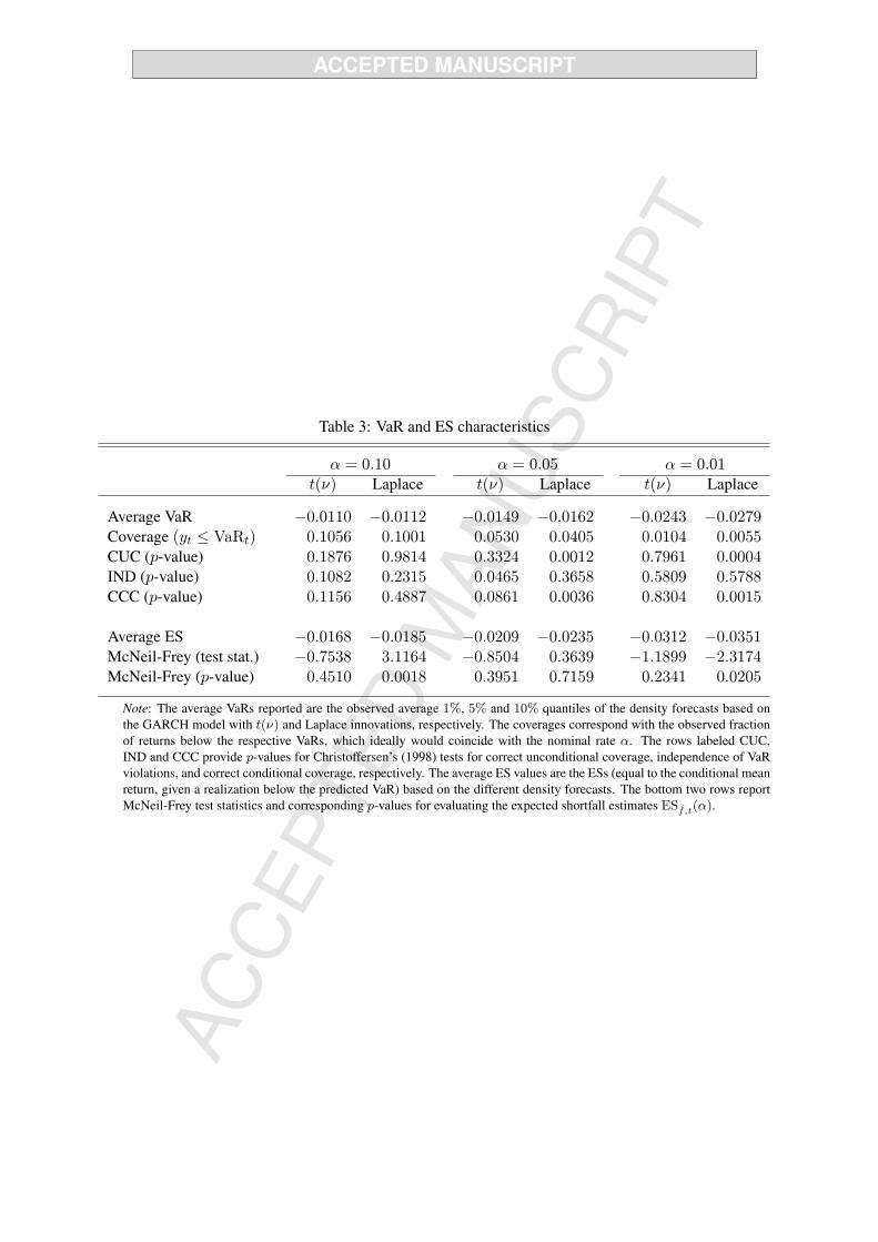
Table 3: VaR and ES characteristics
α = 0.10 α = 0.05 α = 0.01t(ν) Laplace t(ν) Laplace t(ν) Laplace
Average VaR −0.0110 −0.0112 −0.0149 −0.0162 −0.0243 −0.0279Coverage (yt ≤ VaRt) 0.1056 0.1001 0.0530 0.0405 0.0104 0.0055CUC (p-value) 0.1876 0.9814 0.3324 0.0012 0.7961 0.0004IND (p-value) 0.1082 0.2315 0.0465 0.3658 0.5809 0.5788CCC (p-value) 0.1156 0.4887 0.0861 0.0036 0.8304 0.0015
Average ES −0.0168 −0.0185 −0.0209 −0.0235 −0.0312 −0.0351McNeil-Frey (test stat.) −0.7538 3.1164 −0.8504 0.3639 −1.1899 −2.3174McNeil-Frey (p-value) 0.4510 0.0018 0.3951 0.7159 0.2341 0.0205
Note: The average VaRs reported are the observed average 1%, 5% and 10% quantiles of the density forecasts based onthe GARCH model with t(ν) and Laplace innovations, respectively. The coverages correspond with the observed fractionof returns below the respective VaRs, which ideally would coincide with the nominal rate α. The rows labeled CUC,IND and CCC provide p-values for Christoffersen’s (1998) tests for correct unconditional coverage, independence of VaRviolations, and correct conditional coverage, respectively. The average ES values are the ESs (equal to the conditional meanreturn, given a realization below the predicted VaR) based on the different density forecasts. The bottom two rows reportMcNeil-Frey test statistics and corresponding p-values for evaluating the expected shortfall estimates ESf ,t(α).

0
0.1
0.2
0.3
0.4
0.5
de
nsity
N(0,1)stand. t(5)
-3-2.5
-2-1.5
-1-0.5
0 0.5
-4 -3 -2 -1 0 1 2 3 4
log
lik
elih
oo
d r
atio
y
Figure 1: Probability density functions of the standard normal distribution ft(yt+1) and standard-ized Student-t(5) distribution gt(yt+1) (upper panel) and corresponding relative log-likelihood scoreslog ft(yt+1)− log gt(yt+1) (lower panel).

0
0.2
0.4
0.6
0.8
1
-0.005 0 0.005
empi
rical
CD
F
score
wlcl
csl
Figure 2: Empirical CDFs of mean relative scores d∗m,n for the weighted logarithmic (wl) scoring rule
in (4), the conditional likelihood (cl) in (11), and the censored likelihood (csl) in (12) for series ofn = 2, 000 independent observations from a standard normal distribution. The scoring rules are basedon the threshold weight function wt(y) = I(y ≤ r) with r = −2.5. The relative score is defined as thescore for the (correct) standard normal density minus the score for the standardized Student-t(5) density.The graph is based on 10, 000 replications.

0
0.2
0.4
0.6
0.8
1
0 0.005
em
piric
al C
DF
score
(a=3)
clcsl
0
0.2
0.4
0.6
0.8
1
0 0.005
em
piric
al C
DF
score
(a=4)
clcsl
0
0.2
0.4
0.6
0.8
1
0 0.005
em
piric
al C
DF
score
(a=6)
clcsl
0
0.2
0.4
0.6
0.8
1
0 0.005
em
piric
al C
DF
score
(a=10)
clcsl
Figure 3: Empirical CDFs of mean relative scores d∗m,n for the generalized conditional likelihood (cl)
and censored likelihood (csl) scoring rules for series of n = 2, 000 independent observations from astandard normal distribution. The scoring rules are based on the logistic weight function wt(y) definedin (13) for various values of the slope parameter a. The relative score is defined as the score for (correct)standard normal density minus the score for the standardized Student-t(5) density. The graph is basedon 10, 000 replications.
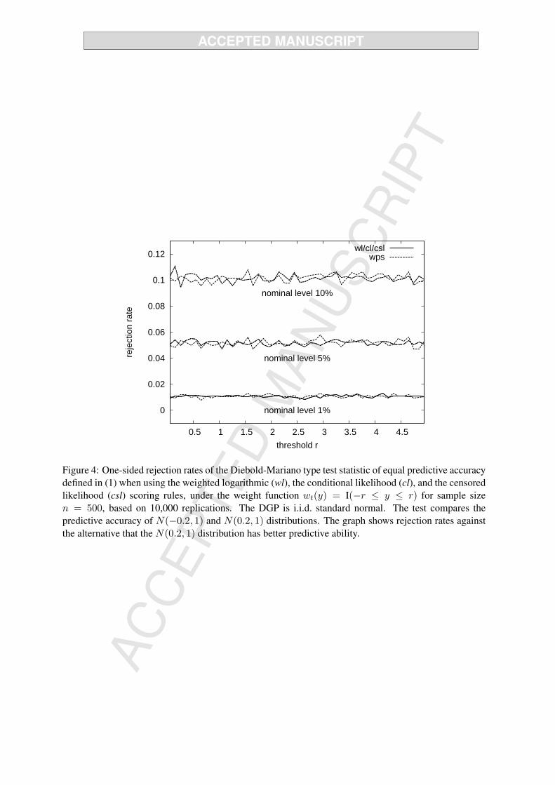
0
0.02
0.04
0.06
0.08
0.1
0.12
0.5 1 1.5 2 2.5 3 3.5 4 4.5
reje
ctio
n ra
te
threshold r
nominal level 1%
nominal level 5%
nominal level 10%
wl/cl/cslwps
Figure 4: One-sided rejection rates of the Diebold-Mariano type test statistic of equal predictive accuracydefined in (1) when using the weighted logarithmic (wl), the conditional likelihood (cl), and the censoredlikelihood (csl) scoring rules, under the weight function wt(y) = I(−r ≤ y ≤ r) for sample sizen = 500, based on 10,000 replications. The DGP is i.i.d. standard normal. The test compares thepredictive accuracy of N(−0.2, 1) and N(0.2, 1) distributions. The graph shows rejection rates againstthe alternative that the N(0.2, 1) distribution has better predictive ability.

0
0.2
0.4
0.6
0.8
1
-3 -2 -1 0 1 2 3
reje
ctio
n ra
te
threshold r
wlwps
clcsl
0
0.2
0.4
0.6
0.8
1
-3 -2 -1 0 1 2 3
reje
ctio
n ra
te
threshold r
wlwps
clcsl
0
0.2
0.4
0.6
0.8
1
-4 -3 -2 -1 0 1 2 3 4
reje
ctio
n ra
te
threshold r
wlwps
clcsl
0
0.2
0.4
0.6
0.8
1
-4 -3 -2 -1 0 1 2 3 4
reje
ctio
n ra
te
threshold r
wlwps
clcsl
Figure 5: One-sided rejection rates (at nominal significance level 5%) of the Diebold-Mariano typetest statistic of equal predictive accuracy defined in (1) when using the weighted logarithmic (wl), theconditional likelihood (cl), and the censored likelihood (csl) scoring rules, under the threshold weightfunction wt(y) = I(y ≤ r) for c = 5 expected observations in the region of interest, based on 10,000replications. For the graphs in the left and right columns, the DGP is i.i.d. standard normal and i.i.d.standardized Student-t(5), respectively. The test compares the predictive accuracy of the standard normaland the standardized Student-t(5) distributions. The graphs in the top (bottom) panels show rejectionrates against superior predictive ability of the standard normal (standardized Student-t(5)) distribution,as a function of the threshold parameter r.
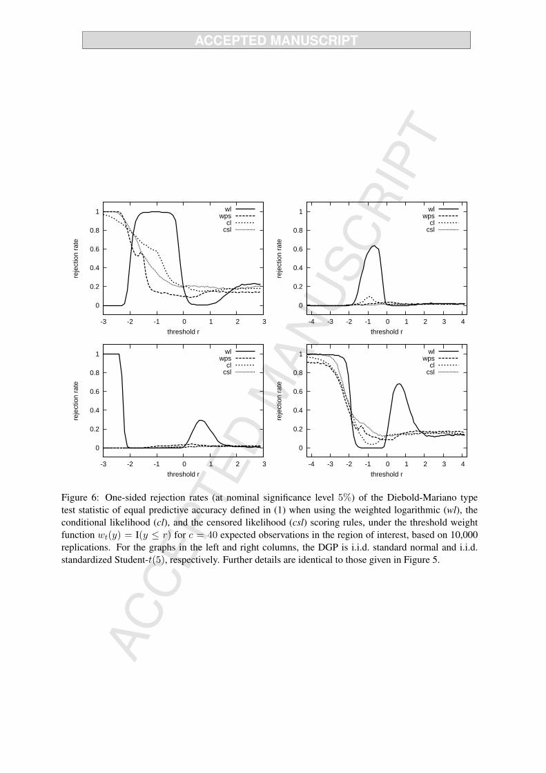
0
0.2
0.4
0.6
0.8
1
-3 -2 -1 0 1 2 3
reje
ctio
n ra
te
threshold r
wlwps
clcsl
0
0.2
0.4
0.6
0.8
1
-3 -2 -1 0 1 2 3
reje
ctio
n ra
te
threshold r
wlwps
clcsl
0
0.2
0.4
0.6
0.8
1
-4 -3 -2 -1 0 1 2 3 4
reje
ctio
n ra
te
threshold r
wlwps
clcsl
0
0.2
0.4
0.6
0.8
1
-4 -3 -2 -1 0 1 2 3 4
reje
ctio
n ra
te
threshold r
wlwps
clcsl
Figure 6: One-sided rejection rates (at nominal significance level 5%) of the Diebold-Mariano typetest statistic of equal predictive accuracy defined in (1) when using the weighted logarithmic (wl), theconditional likelihood (cl), and the censored likelihood (csl) scoring rules, under the threshold weightfunction wt(y) = I(y ≤ r) for c = 40 expected observations in the region of interest, based on 10,000replications. For the graphs in the left and right columns, the DGP is i.i.d. standard normal and i.i.d.standardized Student-t(5), respectively. Further details are identical to those given in Figure 5.

-0.03
-0.02
-0.01
0
0.01
0.02
0.03
0.04
0.05
-4 -2 0 2 4
mea
n sc
ore
r
Figure 7: Mean relative wl score E[dwlt+1] with threshold weight function wt(y) = I(y ≤ r) for thestandard normal versus the standardized Student-t(5) density as a function of the threshold value r, forthe standard normal DGP.

0
0.2
0.4
0.6
0.8
1
0.5 1 1.5 2 2.5 3 3.5 4 4.5 5
reje
ctio
n ra
te
threshold r
wlwps
clcsl
0
0.2
0.4
0.6
0.8
1
0.5 1 1.5 2 2.5 3 3.5 4 4.5 5
reje
ctio
n ra
te
threshold r
wlwps
clcsl
0
0.2
0.4
0.6
0.8
1
0.5 1 1.5 2 2.5 3 3.5 4 4.5 5
reje
ctio
n ra
te
threshold r
wlwps
clcsl
0
0.2
0.4
0.6
0.8
1
0.5 1 1.5 2 2.5 3 3.5 4 4.5 5
reje
ctio
n ra
te
threshold r
wlwps
clcsl
Figure 8: One-sided rejection rates (at nominal significance level 5%) of the Diebold-Mariano typetest statistic of equal predictive accuracy defined in (1) when using the weighted logarithmic (wl), theconditional likelihood (cl), and the censored likelihood (csl) scoring rules, under the weight functionwt(y) = I(−r ≤ y ≤ r) for c = 200 expected observations in the region of interest, based on 10,000replications. The DGP is i.i.d. standard normal. The graphs on the left and right show rejection ratesagainst better predictive ability of the standard normal distribution compared to the standardized Student-t(5) distribution and vice versa, respectively.

0
0.2
0.4
0.6
0.8
1
0.01 0.1 0.2 0.3 0.4 0.5
reje
ctio
n r
ate
α-quantile threshold
wlwps
clcsl
0
0.2
0.4
0.6
0.8
1
0.01 0.1 0.2 0.3 0.4 0.5
reje
ctio
n r
ate
α-quantile threshold
wlwps
clcsl
Figure 9: One-sided rejection rates (at nominal significance level 5%) of the Diebold-Mariano typetest statistic of equal predictive accuracy defined in (1) when using the weighted logarithmic (wl), theweighted probability wps, the conditional likelihood (cl), and the censored likelihood (csl) scoring rulesfor c = 40 expected observations in the region of interest, based on 1,000 replications. The data followan GARCH(1)-process with the standard normal innovations. The competing model is based on thestandardized Student-t(5) innovations. The graphs on the left and right show rejection rates against betterpredictive ability of the forecast based on the standard normal innovations compared to the forecast basedon standardized Student-t(5) innovations and vice versa, respectively.
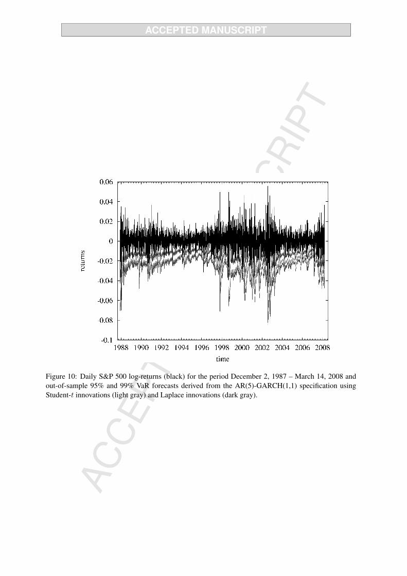
Figure 10: Daily S&P 500 log-returns (black) for the period December 2, 1987 – March 14, 2008 andout-of-sample 95% and 99% VaR forecasts derived from the AR(5)-GARCH(1,1) specification usingStudent-t innovations (light gray) and Laplace innovations (dark gray).