Limited Information and Advertising in the USPersonal Computer Industry

Michelle Sovinsky Goeree1

First version: June, 2002This version: January, 2008

Abstract

Traditional discrete choice models assume buyers are aware of all products for sale. Inmarkets where products change rapidly the full information assumption is untenable. Ipresent a discrete choice model of limited consumer information, where advertising in�uencesthe set of products from which consumers choose to purchase. I apply the model to the USpersonal computer market where top �rms spend over $2 billion annually on advertising.I �nd estimated markups of 19% over production costs, where top �rms advertise morethan average and earn higher than average markups. High markups are explained to alarge extent by informational asymmetries across consumers, where full information modelspredict markups of one-fourth the magnitude. I �nd that estimated product demand curvesare biased towards being too elastic under traditional models. I show how to use data onmedia exposure to improve estimated price elasticities in the absence of micro ad data.

JEL Classi�cation: L15, D12, D21, M37, L63

Keywords: Advertising, information, discrete choice models, product di¤erentiation, per-sonal computer industry

1University of Southern California and Claremont McKenna College (email:michelle.goeree@gmail.com). This paper is based on my 2002 dissertation. Special thanksto my advisors, Steven Stern and Simon Anderson. I am grateful to Costas Meghir and threeanonymous referees for their detailed comments, which substantially improved the paper. Thepaper has bene�ted from comments of seminar partipants at Amsterdam, Arizona, ClaremontMcKenna, Edinburgh, KU Leuven, Southern California, Tilburg, UC Irvine, Virginia, Warwick,Yale, EARIE meetings, and IIOC meetings and discussions with Dan Ackerberg, Steve Berry,Greg Crawford, Jacob Goeree, Phil Haile, Mike Keane, Aviv Nevo, Margaret Slade, Matt Shum,Frank Verboven, and Michael Waterson. I thank Gartner Inc. and Sandra Lahtinen for makingthe data available. I am grateful for �nancial support from the University of Virginia�s BankardFund for Political Economy.

1. Introduction

In 1998 over 36 million personal computers (PCs) were sold in the US, generating over $62

billion in revenues�over $2 billion of which was spent on advertising. The PC industry is

one in which products change rapidly, with approximately 200 new products introduced by

the top 15 �rms every year (Gartner Inc., 1999). Due to the large number of PCs available

and the frequency with which new products are brought into the market, consumers are

unlikely to be aware of all PCs for sale. Furthermore, it is reasonable to suspect consumers

have limited information in many industries.

Traditional random coe¢ cient discrete choice models are estimated under the assumption

that buyers are aware of all available products. Within the full information framework,

Berry, Levinsohn, and Pakes (1995)(hereafter BLP) show that it is important to allow for

consumer taste heterogeneity in order to obtain realistic estimates of demand elasticities.

This paper adds to BLP and shows that it is just as important to allow for heterogeneity in

consumer information in industries with a rapidly changing product line. Indeed, in rapidly

changing markets informational asymmetries may explain (perhaps a signi�cant) part of the

variation in sales.

This paper presents a model of limited information where the imperfect substitutabil-

ity between di¤erent brands may arise from limited consumer information about product

o¤erings as well as from idiosyncratic brand preferences. The limited information model

incorporates three important sources of consumer heterogeneity: choice sets, tastes, and ad-

vertising media exposure. Following the data combining approach of Petrin (2002), I show

how to estimate a model of limited information in the absence of micro-level advertising

data, which are di¢ cult to obtain in many industries.1

The results suggest that traditional models, which rule out non-random informational

asymmetries a priori, can yield estimates of product-speci�c demand curves that are biased

towards being too elastic. The estimates indicate that advertising has very di¤erent infor-

mative e¤ects across individuals and media, and that allowing for heterogeneity in consumer

information yields more realistic estimates of demand elasticities.

The results show that (i) limited information about a product is a contributing factor

to di¤erences in purchase outcomes and (ii) information is distributed across households in

a non-random way. An implication of these �ndings is that assuming full information may

lead to incorrect conclusions regarding the intensity of competition. Indeed, I found high

estimated median markups in the PC industry in 1998, about 19%, whereas traditional full

1Recent structural studies of advertising utilizing micro purchase and advertising exposure data includeErdem and Keane (1996), Ackerberg (2003), and Anand and Shachar (2004). Shum (2004) matches aggregateadvertising data to micro purchase data.

2

information models suggest the industry was more competitive, with estimated markups

of only 5%. Furthermore, the results suggest top �rms bene�t from limited consumer

information with the top �rms earning higher than average markups and engaging in higher

than average advertising. These implications are of particular importance when addressing

policy issues.

The paper proceeds as follows, in the next section I describe the data. I discuss the

model and identi�cation in sections 3 and 4. Estimation is discussed in section 5. The

results from preliminary regressions and from the full model are presented in sections 6 and

7, respectively. I describe the speci�cation tests and conclude in the �nal sections 8 and 9.

2. Data

Product Level Data The product level data were provided by Gartner Inc. and consist

of quarterly shipments and dollar sales of all PCs sold between 1996 and 1998.2 The majority

of �rms sell to the home market, businesses, educational institutions, and the government.

Since the focus of this research is on consumer behavior, I use the home market data to

estimate the model.3 Sales to the home market comprise over 30% of all PCs sold.

As can be seen from Table I, the PC industry is concentrated, with the top six �rms

accounting for over 69% (71%) of the dollar (unit) home market share on average. The

major market players did not change over the period, although there was signi�cant change

in some of their market shares. The top ten �rms, based on home market share (Acer,

Apple, Compaq, Dell, Gateway, Hewlett-Packard, IBM, Micron, NEC, and Packard-Bell),

account for over 80% of PC sales to the home market. The analysis includes the top ten

�rms and �ve others (AST, AT&T / NCR, DEC, Epson, and Texas Instruments) to make

full use of micro-purchase data.4 The 15 �included��rms account for over 85% (83%) of

the dollar (unit) home market share on average.

I have data on �ve main PC attributes: manufacturer (e.g. Dell), brand (e.g. Latitude

LX), form factor (e.g. desktop), CPU type (e.g. Pentium II), and CPU speed (MHz). I

de�ne a model as a manufacturer, brand, CPU type, CPU speed, form factor combination.

Due to data limitations, I do not include some essential product characteristics (such as

memory or hard disk) or product peripherals (such as CD-ROM or modem). However, the

2Prices are dollar sales divided by units sold and are de�ated using the Consumer Price Index from BLS.3I use the non-home sector data in the supply side of the model (see section 3.3).4While all �rms were active in 1996, by 1998, Texas Instruments had merged with Acer, DEC had merged

with Compaq, and the other three �rms had disappeared from the home market. I treat changes in numberof products and �rms as exogenous variation, a common assumption made in this literature. I discuss theimpact of including the smaller �rms on the results in section 8.

3

ease with which consumers can add on after purchase (by buying RAM or a CD-ROM, for

instance) would make it di¢ cult to determine consumer preferences over these dimensions.

The data I use consist of a more limited set of attributes, but those which cannot be easily

altered after purchase. The Gartner data still allow for a very narrow model de�nition.

For example, the Compaq Armada 6500 and the Armada 7400 are two separate models.

Both have Pentium II 300/366 processors, 64 MB standard memory, 56KB/s modem, an

expansion bay for peripherals, and full-size displays and keyboards. The 7400 is lighter,

although somewhat thicker, and it has a larger standard hard drive, and more cache memory.

In both models the hard drive and memory are expandable up to the same limit. In addition,

the Apple Power Macintosh Power PC 604 180/200 desktop and deskside are two separate

models. They di¤er only in their form factor.

Percentage Dollar Median Percentage MarkupManufacturer Home Market Share Ad Ad to Sales Median Price over Marginal Costs including ad costs

1996 1997 1998 Expend Ratio Home Sector Home Sector Home SectorIndustry 3.4% $2,239 15% 10%

Top 6 Firm 65.67 68.31 75.26 $469 9.1% $2,172 17% 12%

Acer 6.20 6.02 4.37 $117 5.4% $1,708 11% 9%Apple 6.66 5.79 9.16 $161 5.3% $1,859 16% 9%AST 3.08 1.53 13%Compaq 11.89 16.29 16.43 $208 2.4% $2,070 23% 16%Dell 2.46 2.87 2.57 $150 2.1% $2,297 10%Gateway 8.94 11.77 16.43 $277 5.6% $2,767 12% 10%Hewlett­Packard 4.02 5.52 10.05 $651 17.7% $2,203 16% 10%IBM 8.49 7.42 6.85 $1,189 20.1% $2,565 16% 10%Micron 3.26 4.05 1.68 7%NEC 3.22Packard Bell 23.48Packard Bell ­ NEC 21.02 16.33 $327 7.2% $2,075 16% 11%Texas Instruments 1.40 7%

15 included 83.11 82.27 83.88

Notes:Others in the 15 included are ATT(NCR), DEC, and Epson, each of which held less than 1% of the home (and total) market shares in 1996 and 1997. AST and Micronheld less than 1% total market shares on average. In 1997 three mergers occurred :Packard Bell, NEC,ZDS; Acer,Texas Instr.; Gateway, Advanced Logic Research.Ad expenditures (in $M) and ad to sales ratios are annual averages and are from LNA and include all sectors (home, business, education, government).  Percentage markupsare the median (price­marginal costs)/price across all products. The last column is percentage total markups per unit after including advertising. These are determined fromestimated markups and estimated effective product advertising in the home sector.

Average Annual

Table I: Summary Statistics for Market Shares, Advertising, Prices, and Markups

Treating a model/quarter as an observation, the sample size is 2112,5 representing 723

distinct models. The majority of the PCs o¤ered to home consumers were desk PCs (70%)

and over 83% of the processors were Pentium-based. The number of models o¤ered by

each �rm varied. Compaq had the largest selection with 138 di¤erent choices, while Texas

Instruments o¤ered only �ve. On average, each �rm o¤ered a model for three quarters.

The market size is the number of US households in a given period, as reported by the

Census Bureau. Market shares are unit sales of each model divided by market size. The

outside good market share is one minus the share of the inside goods.

5This is the sample size after eliminating observations with negligible quarterly market shares.

4

Advertising Data Due to data limitations, previous studies were unable to consider the

di¤erential e¤ects of advertising across media. I use advertising data from Competitive

Media Reporting�s (CMR) LNA/ Multi-Media publication, which includes quarterly ad ex-

penditures across ten media. Some of the media channels are not used frequently by PC

�rms. For example, outdoor advertising for PCs is rare (on average less than 0.3% of ad

expenditures). I aggregate the media into newspaper, magazine, television (TV) and radio

categories.6 These broader channels contain more non-zero observations aiding identi�cation

of media speci�c parameters.

These data are not broken down by sector (e.g. home, business, etc.). CMR categorizes

advertising across product types, which, in some instances, allows me to isolate non-home

expenditures. For example, some expenditures are reported with detail, (e.g. IBM RS/6000

server) while others are generally reported (e.g. IBM various computers). As a result, the

ad measure includes some expenditures on non-PC systems intended for non-home sectors

(such as mainframe servers and UNIX workstations).

Total ad expenditures by the top �rms in the computer industry have grown from $1.4

billion in 1995 to over $2 billion in 1998 (an average annual rate close to 13%). As Table I

shows, there is much variation across �rms. The industry ad-to-sales ratio is 3.4%. However,

the top �rms spend on average over 9% of their sales revenue on advertising. Notably, the

majority of the top �rm expenditures are by IBM whose ad-to-sales ratio is over 20%. IBM�s

large relative ad expenditures may be due to its non-PC interests (servers, mainframes, UNIX

workstations, etc.). To examine this hypothesis, in the model, I allow the position of the

�rm in the non-PC sector to a¤ect the non-home sector marginal revenue of advertising.

Excluding IBM�s expenditures, the remaining top �rms spend an average of 6.5% of their

revenue on advertising. In contrast, Compaq�s ad-to-sales ratio is only 2.4%.

It is common for PC �rms to advertise products simultaneously in groups. For example,

in 1996, one of Compaq�s ad campaigns involved all Presarios (of which there are 12). One

possibility is that group advertising provides as much information about the products in

the group as product-speci�c advertising. However, if group advertising were as e¤ective

as product advertising, we would observe only group advertising (the most e¢ cient use of

resources). An alternative possibility is that group advertising merely informs the consumer

about the �rm. If this were the case, we should observe either �rm-level (the largest possible

group) or product-speci�c advertising.

In reality, �rms use a combination of product-speci�c and group advertising (with groups

of varying sizes). I need a measure of ad expenditures by product that incorporates all

6The �magazine�medium includes Sunday magazines. The �television�medium includes network, spot,cable or syndicated TV. The �radio� medium includes network and spot radio. There are many zeroobservations for outdoor advertising, and so I choose to add it to the radio medium.

5

advertising done for the product. I construct �e¤ective�product ad expenditures by adding

observed product-speci�c expenditures to a weighted average of all group expenditures for

that product where the weights are estimated. Let Gj be the set of all product groupsthat include product j (I suppress the time subscript). Let adH be (observed) total ad

expenditures for group H 2 Gj where the average expenditure per product in the group is

adH �adHjHj :

Then �e¤ective�ad expenditures for product j are given by

adj =XH2Gj

��1adH + �2ad

2

H

�(1)

where the sum is over the di¤erent groups that include product j:7 This speci�cation allows

for increasing or decreasing returns to group advertising. If there is only one product in the

group (i.e. it is product-speci�c), I restrict �1 to unity and �2 to zero.

Consumer Level Data The consumer level data come from the Survey of Media and

Markets conducted by Simmons Market Research Bureau. Simmons collects data on con-

sumers�media habits, product usage, and demographics from about 20,000 households an-

nually. Ideally, one would have individual-level purchase, ad exposure, and demographic

data. Unfortunately, these data are not available for the PC industry. However, I am able

to use the Simmons data to link demographics with purchases and to control for household

variation in advertising media exposure. I use two years of the survey from 1996-1997 (data

from 1998 were not publicly available). Descriptive statistics are given in Table II.8

The Simmons respondents were asked about their media habits. I use the self-reported

media exposure information to control for variation in advertising media exposure across

households. I combine the Simmons data with (separate) information on market shares

and product characteristics, which enables me to obtain a more precise picture of how media

exposure and demand are related. I use these data to construct �media exposure�moments.

In addition, Simmons collects information on PC ownership, including whether the in-

dividual purchased in the past year and the manufacturer. Approximately 11% of the

households purchased a PC in the last 12 months. Respondents were not asked any speci�cs

7I call these �e¤ective� product ad expenditures to indicate they are constructed from observed groupand product-speci�c advertising. To get an idea of the level of detail in the data: in the �rst quarter of1998, there were 18 group advertisements for Apple computers. The groups advertised ranged from �variouscomputers�to �PowerBook�to �Macintosh Power PC G3 Portable�(the later being a speci�c model). Inthis quarter the Apple Macintosh Power PC G3 Portable computer belonged to 7 di¤erent product groups.

8The Simmons survey oversamples in large metropolitan areas. This causes no estimation bias becauseresidential location is treated as exogenous. To reduce the sample to a manageable size, I select 6700respondents randomly from each year. The �nal sample size is 13,400.

6

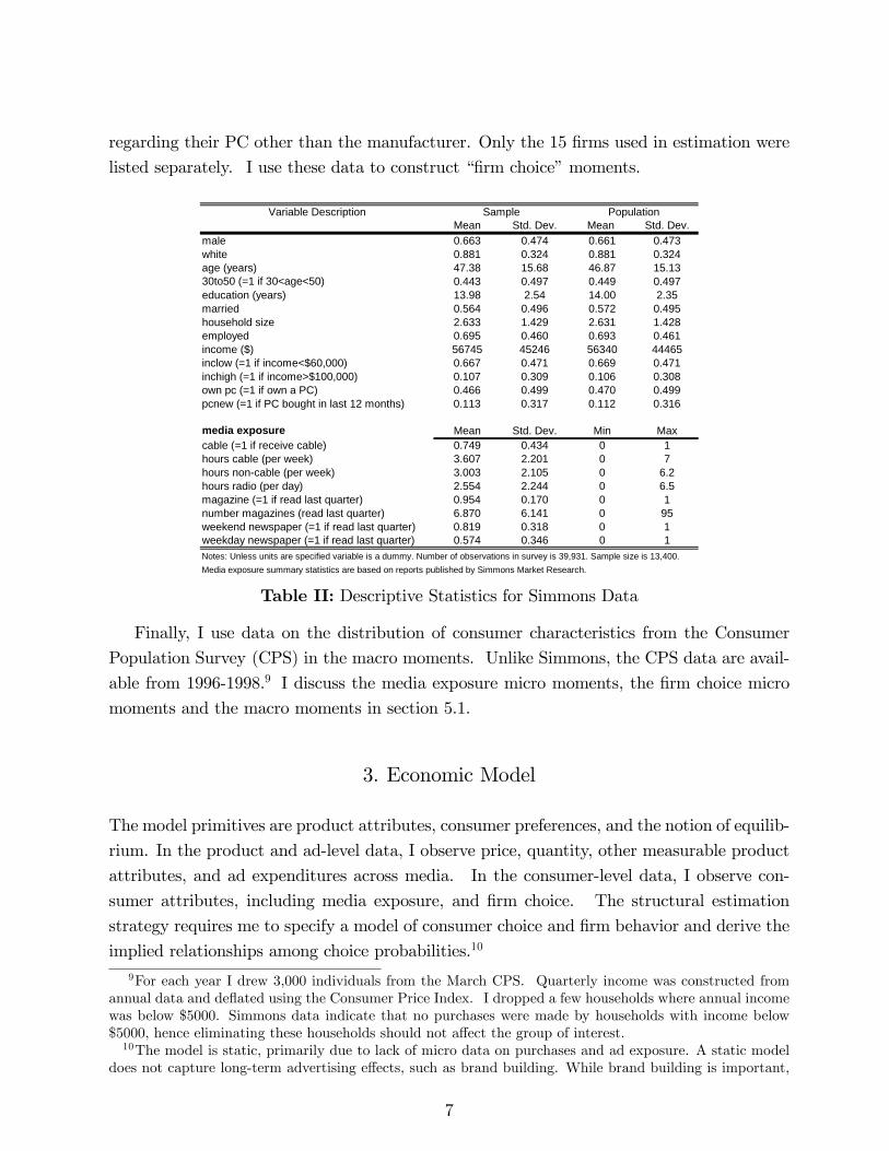
regarding their PC other than the manufacturer. Only the 15 �rms used in estimation were

listed separately. I use these data to construct ��rm choice�moments.

Variable Description Sample PopulationMean Std. Dev. Mean Std. Dev.

male 0.663 0.474 0.661 0.473white 0.881 0.324 0.881 0.324age (years) 47.38 15.68 46.87 15.1330to50 (=1 if 30<age<50) 0.443 0.497 0.449 0.497education (years) 13.98 2.54 14.00 2.35married 0.564 0.496 0.572 0.495household size 2.633 1.429 2.631 1.428employed 0.695 0.460 0.693 0.461income ($) 56745 45246 56340 44465inclow (=1 if income<$60,000) 0.667 0.471 0.669 0.471inchigh (=1 if income>$100,000) 0.107 0.309 0.106 0.308own pc (=1 if own a PC) 0.466 0.499 0.470 0.499pcnew (=1 if PC bought in last 12 months) 0.113 0.317 0.112 0.316

media exposure Mean Std. Dev. Min Maxcable (=1 if receive cable) 0.749 0.434 0 1hours cable (per week) 3.607 2.201 0 7hours non­cable (per week) 3.003 2.105 0 6.2hours radio (per day) 2.554 2.244 0 6.5magazine (=1 if read last quarter) 0.954 0.170 0 1number magazines (read last quarter) 6.870 6.141 0 95weekend newspaper (=1 if read last quarter) 0.819 0.318 0 1weekday newspaper (=1 if read last quarter) 0.574 0.346 0 1Notes: Unless units are specified variable is a dummy. Number of observations in survey is 39,931. Sample size is 13,400.Media exposure summary statistics are based on reports published by Simmons Market Research.

Table II: Descriptive Statistics for Simmons Data

Finally, I use data on the distribution of consumer characteristics from the Consumer

Population Survey (CPS) in the macro moments. Unlike Simmons, the CPS data are avail-

able from 1996-1998.9 I discuss the media exposure micro moments, the �rm choice micro

moments and the macro moments in section 5.1.

3. Economic Model

The model primitives are product attributes, consumer preferences, and the notion of equilib-

rium. In the product and ad-level data, I observe price, quantity, other measurable product

attributes, and ad expenditures across media. In the consumer-level data, I observe con-

sumer attributes, including media exposure, and �rm choice. The structural estimation

strategy requires me to specify a model of consumer choice and �rm behavior and derive the

implied relationships among choice probabilities.10

9For each year I drew 3,000 individuals from the March CPS. Quarterly income was constructed fromannual data and de�ated using the Consumer Price Index. I dropped a few households where annual incomewas below $5000. Simmons data indicate that no purchases were made by households with income below$5000, hence eliminating these households should not a¤ect the group of interest.10The model is static, primarily due to lack of micro data on purchases and ad exposure. A static model

does not capture long-term advertising e¤ects, such as brand building. While brand building is important,

7

3.1. Utility and Demand

An individual chooses from J products, indexed j = 1; :::; J , where a product is a PC

model de�ned as a �rm-brand-CPU type-CPU speed-form factor combination. Product j

characteristics are price (p), non-price observed attributes (x) (CPU speed, Pentium CPU,

�rm, laptop form factor, etc.), and attributes unobserved to the researcher but known to

consumers and producers (�).11 The indirect utility consumer i obtains from j at time t is

uijt = �jt + �ijt + �ijt

where �jt = x0j� + �jt captures the base utility every consumer derives from j and mean

preferences for xj are captured by �.12 The composite random shock, �ijt + �ijt;13 captures

heterogeneity in consumers�tastes for product attributes, and �ijt is a mean zero stochastic

term distributed i.i.d. type I extreme value across products and consumers.

The �ijt term includes interactions between observed consumer attributes (Dit); unob-

served (to the econometrician) consumer tastes (�i); and xj. Speci�cally,

�ijt = � ln(yit � pjt) + xj0(Dit + ��i) �i � N(0; Ik): (2)

The matrix measures how tastes vary with xj: I assume that �i are independently normally

distributed with a variance to be estimated. � is a scaling matrix. Income is yit:

Consumers have an �outside� option, which includes nonpurchase, purchase of a used

PC, or purchase of a new PC from a �rm not in the 15 included �rms. Normalizing p0t to

zero, the indirect utility from the outside option is

ui0t = � ln(yit) + �0t + �i0t:

I also normalize �0t to zero, because I cannot identify relative utility levels.

3.2. Information Technology

In industries where new product introductions are frequent, the full information assumption

is not innocuous. This paper considers a model of random choice sets, where the probability

the majority of PC �rms have not changed over the period and most had been in existence for many yearsprior to 1996. These �rms would not have as much need to establish a brand image as to spread informationabout new products. The static framework permits me to focus on the in�uence of advertising on the choiceset absent the additional structure and complications of a dynamic setting. Also, the nature of advertisingin the PC industry lends itself to a static framework. Products change rapidly, and the e¤ects of advertisingtoday on future information provision are minimal since the same products are no longer for sale.11I do not include brand �xed e¤ects because there are over 200 brands.12Note that this indirect utility can be derived from a Cobb-Douglas utility function (see BLP).13Choices are invariant to multiplication by a person-speci�c constant, so I �x the standard deviation of

�ijt: Since there are over 2000 products estimating an unrestricted covariance matrix is not feasible.

8

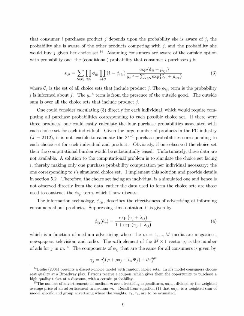
that consumer i purchases product j depends upon the probability she is aware of j, the

probability she is aware of the other products competing with j; and the probability she

would buy j given her choice set:14 Assuming consumers are aware of the outside option

with probability one, the (conditional) probability that consumer i purchases j is

sijt =XS2Cj

Yl2S

�iltYk=2S

(1� �ikt)expf�jt + �ijtg

yit� +P

r2S expf�rt + �irtg(3)

where Cj is the set of all choice sets that include product j: The �ijt term is the probability

i is informed about j. The yit� term is from the presence of the outside good. The outside

sum is over all the choice sets that include product j.

One could consider calculating (3) directly for each individual, which would require com-

puting all purchase probabilities corresponding to each possible choice set. If there were

three products, one could easily calculate the four purchase probabilities associated with

each choice set for each individual. Given the large number of products in the PC industry

(J = 2112), it is not feasible to calculate the 2J�1 purchase probabilities corresponding to

each choice set for each individual and product. Obviously, if one observed the choice set

then the computational burden would be substantially eased. Unfortunately, these data are

not available. A solution to the computational problem is to simulate the choice set facing

i, thereby making only one purchase probability computation per individual necessary: the

one corresponding to i�s simulated choice set. I implement this solution and provide details

in section 5.2. Therefore, the choice set facing an individual is a simulated one and hence is

not observed directly from the data, rather the data used to form the choice sets are those

used to construct the �ijt term, which I now discuss.

The information technology, �ijt, describes the e¤ectiveness of advertising at informing

consumers about products. Suppressing time notation, it is given by

�ij(��) =exp

� j + �ij

�1 + exp

� j + �ij

� (4)

which is a function of medium advertising where the m = 1; :::;M media are magazines,

newspapers, television, and radio. The mth element of the M � 1 vector aj is the numberof ads for j in m.15 The components of �ij that are the same for all consumers is given by

j = a0j('+ �aj + imf ) + #xagej

14Leslie (2004) presents a discrete-choice model with random choice sets. In his model consumers chooseseat quality at a Broadway play. Patrons receive a coupon, which gives them the opportunity to purchase ahigh quality ticket at a discount, with a certain probability.15The number of advertisements in medium m are advertising expenditures, adjm; divided by the weighted

average price of an advertisement in medium m: Recall from equation (1) that adjm is a weighted sum ofmodel speci�c and group advertising where the weights, �1; �2; are to be estimated.

9

where the vectors, ' and �; measure the e¤ectiveness of advertising media at informing

consumers. I include �xed e¤ects for those �rms that o¤ered a product every quarter (the

f ), but do not estimate a �xed e¤ect for each medium, so im is a column vector of ones.

Finally, consumers may be more likely to know a product the longer it has been on the

market, this is captured by # where xagej is the PC age measured in quarters.

Ideally, one would have individual ad exposure data. Unfortunately, these data are

not available for many industries including the PC industry. I control for variation in

household ad exposure (as it is related to observables) by using media exposure information

from Simmons. The �ij captures consumer information heterogeneity:

�ij = a0j(�Dsi � + �i) + eD0

ie� ln�i � N(0; Im):

The � matrix captures how advertising media�s e¤ectiveness varies by observed consumer

characteristics. Simmons data are used to identify�, whereDs is a larger set of demographic

characteristics from the Simmons data.16 Thus �mDsi is the exposure of individual i to

medium m; and a0j�Dsi is the exposure of i to ads for product j: The parameter & measures

the e¤ect of this ad exposure on the information set. The �i vector are unobserved (to the

econometrician) consumer heterogeneity with regard to ad medium e¤ectiveness.17 I assume

� are independent of other unobservables.

In the absence of advertising, consumers still may be (di¤erentially) informed (i.e. �(a =

0) > 0). The eD (a subset of D) proxy for the opportunity costs of acquiring information.18

The magnitude of �ij when no advertising occurs depends on eD0ie�+ #xagej .

Notice �ij depends upon own product advertising only. Allowing informational spillovers

would greatly complicate the model. First, the theoretical framework would have to address

free-riding in advertising choices across �rms. Second, one would need adequate variation

in the data to empirically identify the spillover e¤ect across products. For these reasons,

I assume the probability a consumer is informed about a product is (conditional on her

attributes) independent of the probability she is informed about any other product. Infor-

mation provided (via advertising) for one product (or by one �rm) cannot �spillover� to

another product (or to another �rm). That is, I assume product or group advertising for

product r 6= j provides no information about j.

Let {i = (yi; Di; �i; �i) be the vector of individual characteristics. I assume that the

consumer purchases at most one good per period,19 that which provides the highest util-

ity, U; from all the goods in her choice set. Let Rj � f{ : U({; pj; xj; aj; �j; �ij) �16There are 11 demographic characteristics included in Ds: These are measures of age, household size,

marital status, income, sex, race, and education.17To limit the number of parameters to estimate, I normalized the variance of the � to one for all media.18These consist of dummies for high school graduate, income< $60,000, and income> $100,000.19This assumption may be unwarranted for some products for which multiple purchase is common. How-

10

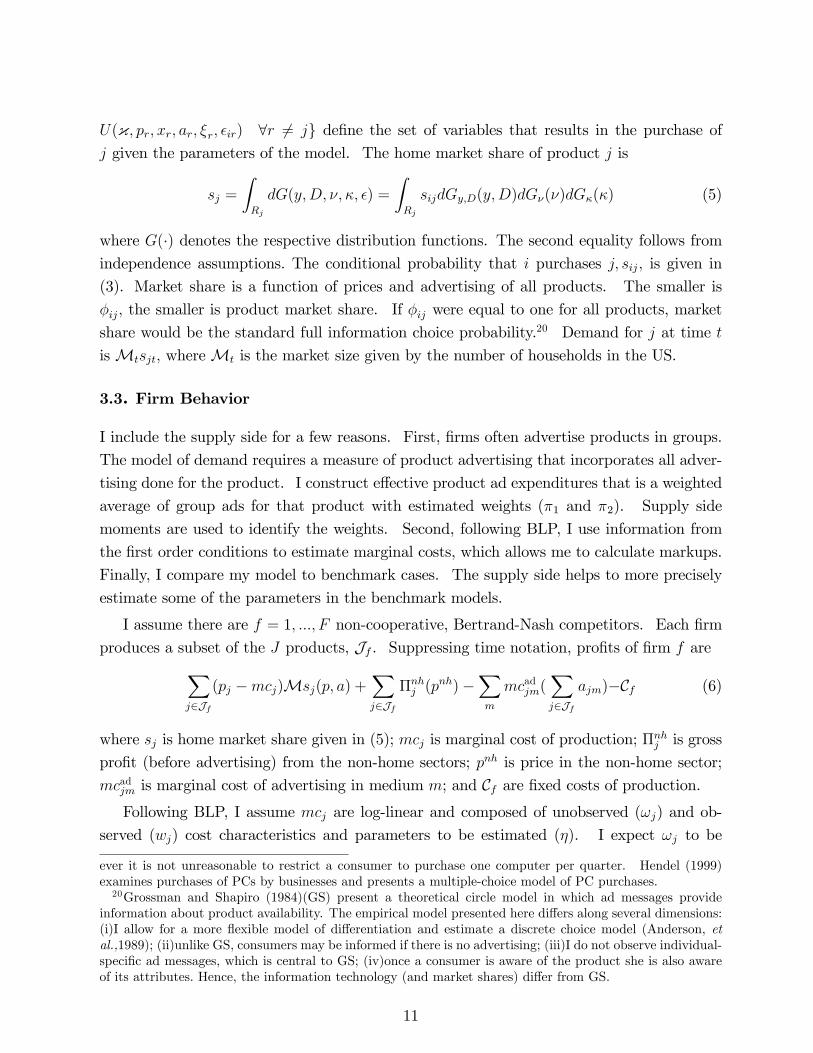
U({; pr; xr; ar; �r; �ir) 8r 6= jg de�ne the set of variables that results in the purchase ofj given the parameters of the model. The home market share of product j is

sj =

ZRj

dG(y;D; �; �; �) =

ZRj

sijdGy;D(y;D)dG�(�)dG�(�) (5)

where G(�) denotes the respective distribution functions. The second equality follows fromindependence assumptions. The conditional probability that i purchases j; sij; is given in

(3). Market share is a function of prices and advertising of all products. The smaller is

�ij; the smaller is product market share. If �ij were equal to one for all products, market

share would be the standard full information choice probability.20 Demand for j at time t

isMtsjt; whereMt is the market size given by the number of households in the US.

3.3. Firm Behavior

I include the supply side for a few reasons. First, �rms often advertise products in groups.

The model of demand requires a measure of product advertising that incorporates all adver-

tising done for the product. I construct e¤ective product ad expenditures that is a weighted

average of group ads for that product with estimated weights (�1 and �2). Supply side

moments are used to identify the weights. Second, following BLP, I use information from

the �rst order conditions to estimate marginal costs, which allows me to calculate markups.

Finally, I compare my model to benchmark cases. The supply side helps to more precisely

estimate some of the parameters in the benchmark models.

I assume there are f = 1; :::; F non-cooperative, Bertrand-Nash competitors. Each �rm

produces a subset of the J products, Jf . Suppressing time notation, pro�ts of �rm f areXj2Jf

(pj �mcj)Msj(p; a) +Xj2Jf

�nhj (pnh)�

Xm

mcadjm(Xj2Jf

ajm)�Cf (6)

where sj is home market share given in (5); mcj is marginal cost of production; �nhj is gross

pro�t (before advertising) from the non-home sectors; pnh is price in the non-home sector;

mcadjm is marginal cost of advertising in medium m; and Cf are �xed costs of production.Following BLP, I assume mcj are log-linear and composed of unobserved (!j) and ob-

served (wj) cost characteristics and parameters to be estimated (�). I expect !j to be

ever it is not unreasonable to restrict a consumer to purchase one computer per quarter. Hendel (1999)examines purchases of PCs by businesses and presents a multiple-choice model of PC purchases.20Grossman and Shapiro (1984)(GS) present a theoretical circle model in which ad messages provide

information about product availability. The empirical model presented here di¤ers along several dimensions:(i)I allow for a more �exible model of di¤erentiation and estimate a discrete choice model (Anderson, etal.,1989); (ii)unlike GS, consumers may be informed if there is no advertising; (iii)I do not observe individual-speci�c ad messages, which is central to GS; (iv)once a consumer is aware of the product she is also awareof its attributes. Hence, the information technology (and market shares) di¤er from GS.

11

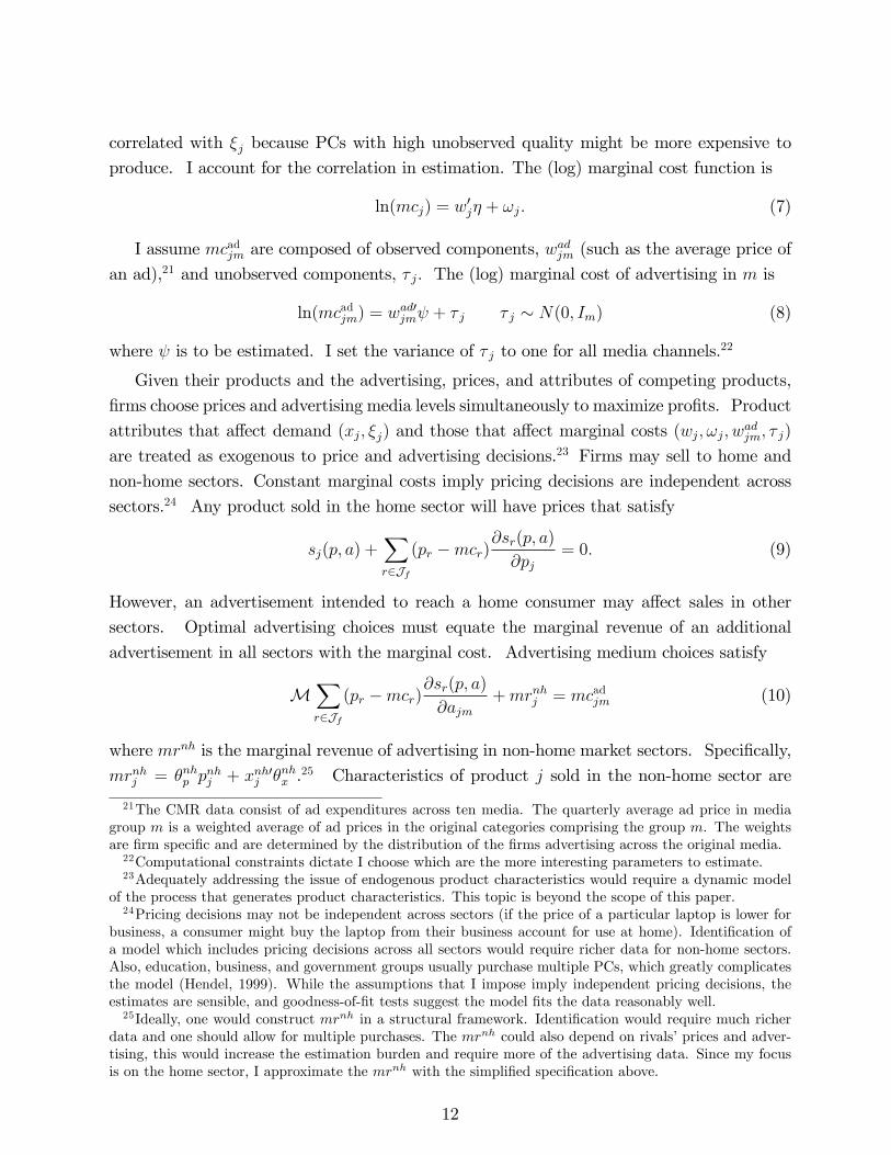
correlated with �j because PCs with high unobserved quality might be more expensive to

produce. I account for the correlation in estimation. The (log) marginal cost function is

ln(mcj) = w0j� + !j: (7)

I assume mcadjm are composed of observed components, wadjm (such as the average price of

an ad),21 and unobserved components, � j: The (log) marginal cost of advertising in m is

ln(mcadjm) = wad0jm + � j � j � N(0; Im) (8)

where is to be estimated. I set the variance of � j to one for all media channels.22

Given their products and the advertising, prices, and attributes of competing products,

�rms choose prices and advertising media levels simultaneously to maximize pro�ts. Product

attributes that a¤ect demand (xj; �j) and those that a¤ect marginal costs (wj; !j; wadjm; � j)

are treated as exogenous to price and advertising decisions.23 Firms may sell to home and

non-home sectors. Constant marginal costs imply pricing decisions are independent across

sectors.24 Any product sold in the home sector will have prices that satisfy

sj(p; a) +Xr2Jf

(pr �mcr)@sr(p; a)

@pj= 0: (9)

However, an advertisement intended to reach a home consumer may a¤ect sales in other

sectors. Optimal advertising choices must equate the marginal revenue of an additional

advertisement in all sectors with the marginal cost. Advertising medium choices satisfy

MXr2Jf

(pr �mcr)@sr(p; a)

@ajm+mrnhj = mcadjm (10)

where mrnh is the marginal revenue of advertising in non-home market sectors. Speci�cally,

mrnhj = �nhp pnhj + xnh0j �nhx .

25 Characteristics of product j sold in the non-home sector are

21The CMR data consist of ad expenditures across ten media. The quarterly average ad price in mediagroup m is a weighted average of ad prices in the original categories comprising the group m. The weightsare �rm speci�c and are determined by the distribution of the �rms advertising across the original media.22Computational constraints dictate I choose which are the more interesting parameters to estimate.23Adequately addressing the issue of endogenous product characteristics would require a dynamic model

of the process that generates product characteristics. This topic is beyond the scope of this paper.24Pricing decisions may not be independent across sectors (if the price of a particular laptop is lower for

business, a consumer might buy the laptop from their business account for use at home). Identi�cation ofa model which includes pricing decisions across all sectors would require richer data for non-home sectors.Also, education, business, and government groups usually purchase multiple PCs, which greatly complicatesthe model (Hendel, 1999). While the assumptions that I impose imply independent pricing decisions, theestimates are sensible, and goodness-of-�t tests suggest the model �ts the data reasonably well.25Ideally, one would construct mrnh in a structural framework. Identi�cation would require much richer

data and one should allow for multiple purchases. The mrnh could also depend on rivals�prices and adver-tising, this would increase the estimation burden and require more of the advertising data. Since my focusis on the home sector, I approximate the mrnh with the simpli�ed speci�cation above.

12

price (pnhj ) and other observable characteristics (xnhj ) including advertising, CPU speed, and

non-PC �rm sales.26 The �nh are parameters to be estimated. Let �AD = fvec( ); vec(�nh)g.

4. Identi�cation

Following the literature, I assume that the demand and pricing unobservables (evaluated at

the true parameter values, �0) are mean independent of a set of exogenous instruments; z :

E��j(�0) j z

�= E [!j(�0) j z] = 0: (11)

I do not observe �j or !j, but market participants do. This leads to endogeneity problems

because prices and ad choices are most likely functions of unobserved characteristics. If

price is positively correlated with unobserved quality, price coe¢ cients (in absolute value)

will be understated (as preliminary estimates in section (6) indicate). Whereas if advertising

is positively correlated with quality, its e¤ect will be overstated.27

A solution involves instrumental variables.28 BLP show that variables that shift markups

are valid instruments for price in di¤erentiated products models. In a limited information

framework the components of z include the characteristics of all the products marketed (the

x), variables that determine production costs (the components of the w that are not in x)

and variables that determine advertising costs (the components of wad).29 The value of the

instrument for any given product can be any function of z:

The intuition to motive the advertising instruments is similar to that used by BLP to

motivate the price instruments. Products which face more competition (due to many rivals

o¤ering similar products) will tend to have lower markups relative to more di¤erentiated

products. Advertising for j depends on j�s markup. As ad �rst order conditions (FOC)

in (10) indicate, a �rm will advertise a product more the more they make on the sale of

the product, ceteris paribus. The pricing FOCs in (9) show the optimal price (and hence

markup) for j depends upon characteristics of all of the products o¤ered. Therefore, the

optimal price and advertising depends upon the characteristics, prices, and advertising of

all products o¤ered. Note also that the level of advertising for j in media m depends on

26Non-PC sales are constructed by subtracting quarterly PC sales from quarterly total manufacturer sales(as recorded in �rm quarterly reports). Therefore �non-home sales�include sales of computer systems suchas mainframes, servers, and UNIX workstations.27See Milgrom and Roberts (1986).28Berry (1994) was the �rst to discuss the implementation of instrumental variables methods to correct

for endogeneity between unobserved characteristics and prices. BLP provide an estimation technique. Mymodel and estimation strategy is in this spirit but is adapted to correct for advertising endogeneity.29Variables that determine production costs that are not in x include a time trend. Hence, production

costs shifters do not play a large role in identifying demand in the model presented in section (3).

13

the marginal cost of advertising in that media: Thus the instruments will be functions of

attributes, product cost shifters, and advertising cost shifters of all other products.

Given (11) and regularity conditions, the optimal instrument for any disturbance-parameter

pair is the expected value of the derivative of the disturbance with respect to the parameter

(evaluated at �0) (Chamberlain, 1987). Optimal instruments are functions of advertising

and prices. To use the optimal instruments, I would have to calculate the price and ad-

vertising equilibrium for di¤erent f�j; !jg sequences, compute the derivatives at equilibriumvalues, and integrate out over the distribution of the f�j; !jg sequences. This is computa-tionally demanding and requires additional assumptions on the joint distribution (�; !):

I form approximations to the optimal instruments, following BLP(1999), by evaluating

the derivatives at the expected value of the unobservables (� = ! = 0). The instruments

will be biased since the derivatives evaluated at the expected values are not the expected

value of the derivatives. However, the approximations are functions of exogenous data and

are constructed such that they are highly correlated with the relevant functions of prices and

advertising. Hence the exogenous instruments will be consistent estimates of the optimal

instruments.30 Details are in Appendix A.

There is a potential endogeneity problem in the micro data. If a consumer with an a

priori higher tendency to purchase a particular product chooses which media to consult in

the decision process, then media exposure will be correlated with the unobservables. To the

extent that exposure is driven by the intention to buy, exposure and purchase decisions will

be correlated even if ad exposure has no impact on the purchase decision.

To account for the dependence of media exposure on the decision to buy, I would have

to model the decision to engage in a particular media and de�ne the joint probability of

purchase and media exposure as a function of observables and unobservables.31 Estimation

would require richer data and additional assumptions on the distribution of unobservables. I

test for the exogeneity of media exposure (see Smith and Blundell, 1986; Rivers and Vuong,

1988), using purchase and media exposure data from Simmons.32 As instruments for media

exposure I use the cost of access (subscription price) to various media. Details are given in

Appendix B. The tests indicate media exposure endogeneity is not an issue in the data. I

cannot reject the null hypothesis that exposure to newspapers, magazines, and cable televi-

sion is exogenous to the PC purchase decision. Given this motivation, I treat media exposure

30One could use a series approximation (BLP) to construct exogenous instruments. I use the more directapproximation (BLP,1999) since it is more closely tied to the model. Results from logit IV regressionsindicate the instruments are strong and that they address the endogeneity issues.31Anand and Shachar(2004) use micro-level data to estimate a model of TV viewing choices and show how

to overcome the exposure endogeneity problem when consumption decisions also determine ad exposures.32Rivers and Vuong (1988) develop a two-step test for the exogeneity of regressors in limited dependent

variable models. Wooldridge (2002) shows the exogeneity test is valid when the regressor is a binary variable.

14

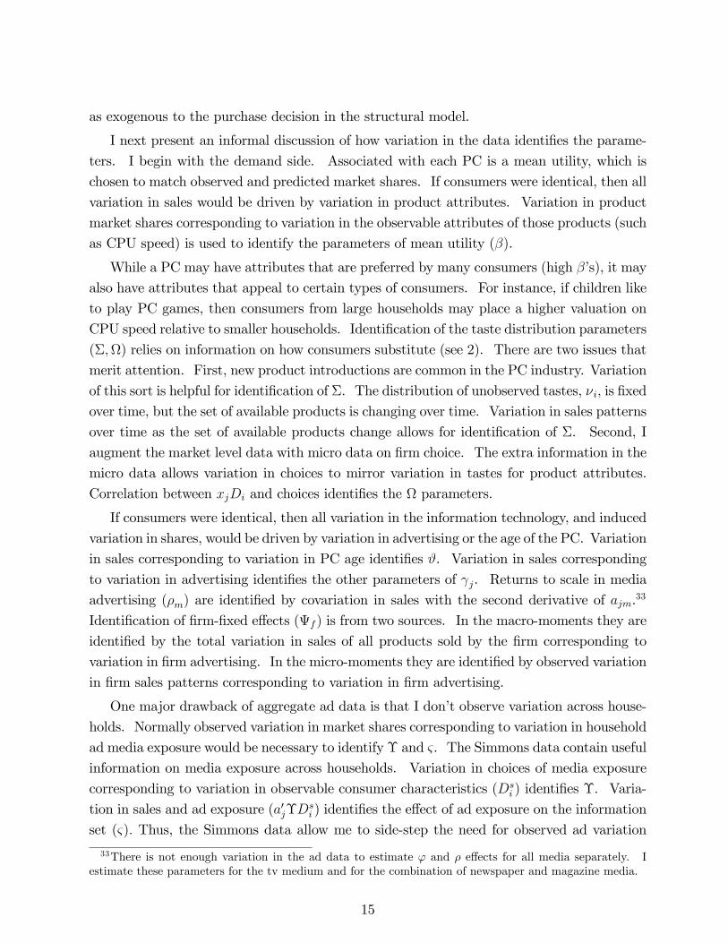
as exogenous to the purchase decision in the structural model.

I next present an informal discussion of how variation in the data identi�es the parame-

ters. I begin with the demand side. Associated with each PC is a mean utility, which is

chosen to match observed and predicted market shares. If consumers were identical, then all

variation in sales would be driven by variation in product attributes. Variation in product

market shares corresponding to variation in the observable attributes of those products (such

as CPU speed) is used to identify the parameters of mean utility (�).

While a PC may have attributes that are preferred by many consumers (high ��s), it may

also have attributes that appeal to certain types of consumers. For instance, if children like

to play PC games, then consumers from large households may place a higher valuation on

CPU speed relative to smaller households. Identi�cation of the taste distribution parameters

(�;) relies on information on how consumers substitute (see 2). There are two issues that

merit attention. First, new product introductions are common in the PC industry. Variation

of this sort is helpful for identi�cation of �. The distribution of unobserved tastes, �i; is �xed

over time, but the set of available products is changing over time. Variation in sales patterns

over time as the set of available products change allows for identi�cation of �. Second, I

augment the market level data with micro data on �rm choice. The extra information in the

micro data allows variation in choices to mirror variation in tastes for product attributes.

Correlation between xjDi and choices identi�es the parameters.

If consumers were identical, then all variation in the information technology, and induced

variation in shares, would be driven by variation in advertising or the age of the PC. Variation

in sales corresponding to variation in PC age identi�es #. Variation in sales corresponding

to variation in advertising identi�es the other parameters of j. Returns to scale in media

advertising (�m) are identi�ed by covariation in sales with the second derivative of ajm.33

Identi�cation of �rm-�xed e¤ects (f ) is from two sources. In the macro-moments they are

identi�ed by the total variation in sales of all products sold by the �rm corresponding to

variation in �rm advertising. In the micro-moments they are identi�ed by observed variation

in �rm sales patterns corresponding to variation in �rm advertising.

One major drawback of aggregate ad data is that I don�t observe variation across house-

holds. Normally observed variation in market shares corresponding to variation in household

ad media exposure would be necessary to identify � and &. The Simmons data contain useful

information on media exposure across households. Variation in choices of media exposure

corresponding to variation in observable consumer characteristics (Dsi ) identi�es �. Varia-

tion in sales and ad exposure (a0j�Dsi ) identi�es the e¤ect of ad exposure on the information

set (&): Thus, the Simmons data allow me to side-step the need for observed ad variation

33There is not enough variation in the ad data to estimate ' and � e¤ects for all media separately. Iestimate these parameters for the tv medium and for the combination of newspaper and magazine media.

15

across households. The other parameters of �ij which do not interact with advertising (e�) areseparately identi�ed from due to nonlinearities. Finally, the parameters on group advertis-

ing (�1 and �2) are identi�ed by observed variation in expenditures on group advertisements

(adm) with the number of products in the group and by functional form.

Variation in prices and shares corresponding to variation in observed cost attributes

identi�es the corresponding cost attributes�e¤ect on production costs. Covariation in ad

prices, advertising and the generalized residuals identi�es the e¤ect of ad prices on ad costs.

5. The Estimation Technique

The econometric technique follows recent studies of di¤erentiated products, such as BLP

(1995, 2004) and Nevo (2000). The parameters are �; � = f�;�;; ��g; �; and �AD; where�� = f�1; �2; '; �;; #; e�;�; &g. Under the assumption that the observed data are the

equilibrium outcomes, I estimate the parameters simultaneously using generalized method

of moments (GMM). There are �ve �sets�of moments:

(i) from demand, which match the predicted market shares to observed shares

(ii) from pricing decisions, which express an orthogonality between the cost side unobserv-able and instruments

(iii) from advertising media decisions, which express an orthogonality between the adver-tising residuals and instruments

(iv) from purchase decisions, which match the model�s predictions for the probability in-dividuals purchase from �rm f (conditional on observed characteristics) to observedpurchases

(v) from media exposure decisions, which match the model�s predictions for exposure tomedia m (conditional on observed characteristics) to observed exposure

5.1. The Moments

I use macro product data, ad data, and the CPS consumer data in the �rst three sets of

moments. I use micro consumer data in the last two sets of moments. The strategy of

combining micro and macro data follows work by Petrin (2002) and BLP(2004).

BLP-Type Macro Moments Following BLP, I restrict the model predictions for j�s

market share to match observed shares. I solve for �(S; �) that is the implicit solution to

Sobst � st(�; �) = 0

16

where Sobst and st are vectors of observed and predicted shares respectively. I substitute

�(S; �) for � when calculating the moments.34 The �rst moment unobservable is

�jt = �jt(S; �)� x0j�: (12)

I use the demand system estimates to compute marginal costs (Bresnahan, 1989). In vector

form, the J FOCs from (9) imply

mc = p��(�; �)�1s(�; �) (13)

where �j;r = �@sr@pjIj;r with Ij;r an indicator function equal to one when j and r are produced

by the same �rm. Combining (13) and (7) yields the second moment unobservable:

! = ln(p��(�; �)�1s(�; �))� w0�: (14)

Advertising Macro Moments Some �rms choose not to advertise some products in some

media. To allow for corner solutions I use the method of generalized residuals proposed by

Gourieroux, et al.(1987). The method is best illustrated by an example. For ease of

exposition I suppress the time subscript. Let y�i = xi� + ui. We observe y�i if y�i � 0

and zero otherwise. The errors, ui(�); are linked with y�i . The errors cannot be used

to construct moments because they depend on unobserved variables. Gourieroux, et al.

suggest an alternative method: replace the errors by their best prediction conditional on the

observable variables, E[ui(�) j yi]; and use these to construct moments.In this paper the latent variables are optimal advertising levels (denoted a�jm): Due to

nonlinearities the application is more complex, but the technique is the same. We observe

ajm =

�a�jm if @�j=@ajm jajm=a�jm= 00 if @�j=@ajm jajm=0< 0

where �j is product j�s pro�t from (6). Rewrite the advertising medium FOC as

ln (mrjm(ajm))� wad0jm = � jm (15)

where mrjm is medium marginal revenue (the left-hand side of (10)). The latent variable is

the implicit solution to (15) so the errors, � jm; will depend on a�jm: I use the best prediction of

� jm; conditional on observed advertising, to construct moments. In estimation, I �x �� = 1:

Using ad marginal costs (8) and the interior FOCs (10), the likelihood function is

$ =Y

j:ajm>0

�normal (fmrjm) Yj:ajm�0

1� � (fmrjm)34I use a contraction mapping suggested by BLP to compute � (S; �) : Goeree (2008) shows that the

function used in the �xed point algorithm is a contraction mapping. The proof parallels the proof for thefull information case.

17

where fmrjm � ln (mrjm(ajm)) � wad0jm ; �normal is the standard normal pdf, and � is the

cumulative standard normal. The generalized residual for the jth observation is

e� jm(b�) = E[� jm(b�) j ajm] = fmrjm1(ajm > 0)� �normal(fmrjm)1� �(fmrjm) 1(ajm = 0)

where � are the parameters of (15) and b� its maximum likelihood estimator.

The (third set of) moments express an orthogonality between the generalized residuals

and the instruments. For instance, the � that solves

1

J

Xj

@fmrjm@�

e� jm = 0is the MOM estimator, where @fmrjm

@�are the appropriate instruments. Let T (�;mc; �; �AD)

be the vector of residuals stacked over media and products.

Firm Choice Micro Moments I combine micro �rm choice data from Simmons with

macro product level data (á la Petrin, 2002).35 The Simmons data connect consumers

to �rms, thus associating consumer and average product attributes (across �rms). These

moments allow me to obtain more precise estimates of the parameters of the taste distribution

( and �) and advertising e¤ectiveness (f). The demographic characteristics for these

moments (denoted Ds) are not given by the CPS but are linked directly to purchases.

Let Bi be a F � 1 vector of �rm choices for individual i. Let bi be a realization of Biwhere bif = 1 if a brand produced by f was chosen. De�ne the residual as the di¤erence

between the vector of observed choices and the model prediction given (�; �) :

Bi(�; �) = bi � E�;�E[Bi j Dsi ; �; �]: (17)

For example, the element of E�;�E[Bi j Dsi ; �; �] corresponding to �rm 2 for consumer i is

Xj2J2

Z XS2Cj

Yl2S

�iltYk=2S

(1� �ikt)expf�jt + �ijtg

yit� +P

r2S expf�rt + �irtgdG�(�)dG�(�)

where the �rst summand is over products sold by �rm 2; the integral is over the assumed

distributions of � and �, and the second summand is over all the di¤erent choice sets that

include product j:36 The population restriction for the micro moment is E[Bi(�; �) j (x; �)] =0: Let B(�; �) be the vector formed by stacking the residuals Bi(�; �) over individuals.35Petrin (2002) shows how to combine macro data with data that links average consumer attributes to

product attributes to obtain more precise estimates.36Simmons is annual so the outermost summand is over all products sold by each �rm over the year.

18

Media ExposureMicroMoments The �fth set of moments are used to estimate�:These

allow me to control for variation in ad exposure across households (as related to observables)

via variation in media exposure. The Simmons respondents were ranked according to how

often they watched TV, read newspapers, etc. relative to others in the surveyed popula-

tion. I have information on the ranges of respondents� answers, but the survey reports

only the quintile to which the consumer belongs. I construct moments arising from an

ordered-response likelihood. Let h�im be the amount of exposure of i to medium m

h�im = Ds0i �m + "im

where "im is a mean zero term distributed i.i.d. standard normal. De�ning quintile one

as the highest, i belongs to the qth quintile in medium m if cqm < h�im < c(q�1)m where c

are cuto¤ values. Let Him be the vector of quintiles for i in m: Let him be a realization of

Him where the qth element himq = 1 if i�s level of exposure falls in q: If � is the cumulative

standard normal and �iqm = �(cqm �Ds0i �m) then

Pr(hiqm = 1) = �i;q�1;m � �iqm:

The maximum likelihood estimate of �m solvesXi

Xq

hiqm@ ln Pr(hiqm = 1 j Ds

i )

@�m= 0:

The di¤erence between the vector of observed quintiles and the prediction given �m;

Him (�m) = him � E [Him j Dsi ;�m] ; (18)

is the residual where the qth element of E [Him j Dsi ;�m] = �iqm � �i;q�1;m and

Zmedia;im =@ ln Pr(hiqm = 1 j Ds

i )

@�md

are the appropriate instruments: Let Hi (�) be the residuals stacked over media.

5.2. The GMM Estimator

I use GMM to �nd the parameter values that minimize the objective function, �0ZA�1Z 0�;

where A is a weighting matrix, which is a consistent estimate of E[Z 0��0Z] and Z are

instruments orthogonal to the composite error term �. Speci�cally, if Z�; Z!; Zad; Zmicro;

Zmedia are the respective instruments for each disturbance/residual, the sample moments are

Z 0� =

26666641J

PJj=1 Z�;j�j(�; �)

1J

PJj=1 Z!;j!j(�; �; �)

1J

Pm�Jj=1 Zad;jTj (�; �; �AD)

1N

PNi=1 Zmicro;iBi(�; �)

1N

PNi=1 Zmedia;iHi (�)

377777519

where Z�;j is column j of Z�: Joint estimation takes into account the cross-equation restric-

tions on the parameters that a¤ect both demand and supply, which yields more e¢ cient

estimates. This comes at the cost of increased computation time since joint estimation

requires a non-linear search over all the parameters of the model.37

Simulation As in BLP, the distribution of consumer demographics is an empirical one.

As a result there is no analytical solution for predicted market shares, making simulation

of equation (5) necessary. Furthermore consumers may not know all products for sale,

but I don�t observe the choice set facing any one consumer. As I discussed in section 3.2,

a solution is to simulate the choice set.38 An outline of the simulation technique follows.

Details are in Appendix C.

I sample a set of �individuals�where each consists of (vi1; : : : ; vik) taste parameters drawn

from a multivariate normal; demographic characteristics, (yi; Di1; : : : ; Did); drawn from the

CPS for use in the macro moments; and unobserved advertising medium e¤ectiveness draws,

(�i1; : : : ; �im); from a multivariate log normal.

Simulating individual i�s choice set is a two-step process. I begin by drawing J uniform

variables for each individual. First, I compute the probability individual i knows product j

for a given value of the parameters. That is I compute the information technology for each

person-product combination (the �ij from equation (4) evaluated at the parameter values).

Second, I compare i�s uniform draw for each product with the computed �ij. If the computed

probability i knows product k (ie. the value of �ik) is larger than the corresponding uniform

draw for k; product k is in i�s choice set. I repeat this comparison for all products and

form i�s simulated choice set. Note that i�s choice set may change as the parameter values

change. I simulate the choice set for the remaining individuals analogously.

Given the simulated choice set, I compute choice probabilities for each individual for

each product and construct an importance sampler to smooth the simulated choice proba-

37I restrict the non-linear search to a subset of the parameters = f�; �ADg. This restriction is possiblesince the FOCs with respect to � and � can be expressed in terms of �. (See Nevo, 2000.) I could separatelyestimate � and substitute predicted for actual exposure when estimating the remaining parameters. Thiswould decrease computational time but, due to the non-linear nature of the model, would not yield consistentestimates except under speci�c distributional assumptions.38Chiang, et al.(1999) use micro purchase data for ketchup to model �consideration set� formation. A

consideration set is a subset of the 2J�1 choice sets. Due to the stable nature of the industry the consumer�sconsideration set doesn�t change over time, allowing the authors to eliminate choice sets which do not containall previously purchased brands. Also, there are only four brands for a consumer to consider. The PC industryis much di¤erent: it is rapidly changing and there are a large number of products. Therefore, I use a verydi¤erent approach in modeling (and estimating) choice set heterogeneity. While the approach I take doesnot a priori limit the potential set of products available to the consumer, the Chiang, et al. approach ismore �exible in the sense that it does not impose conditional independence among products in a particularconsumer�s consideration set. Recent papers addressing consideration sets are Mehta, et al.(2003), Nierop,et al.(2005), and Ching, et al.(2007).

20

bilities.39 The market share simulator is the average over individuals of the smoothed choice

probabilities. The process is similar for the micro moments, but I take R draws for each

product-individual. The individual product choice probability simulator is the average over

the R draws. Individual �rm choice probabilities are the sum over the products o¤ered by

each �rm.

The Estimation Algorithm and Properties of the Estimator First, calculate the

instruments and keep them �xed for the duration of the estimation. Then, given a value of

the parameters, �;

(i) Compute the simulated market shares and solve for the vector � that equates simulatedand observed shares.

(ii) Calculate � and compute the demand unobservables, � (see 12). Calculate � and com-pute the cost side unobservables, ! (see 14). Compute the ad residual, T .

(iii) Simulate the �rm purchase probabilities and calculate the micro residual (see 17).

(iv) Compute the media residual (see 18).

(v) Search for the parameter values that minimize the objective function: b�0ZA�1Z 0b�;where b� is the composite error term resulting from simulated moments. If the para-meters don�t minimize the moments (according to some criteria) make a new guess ofthe parameters. Repeat until moments are close to zero.

The estimator is consistent and asymptotically normal (Pakes and Pollard, 1989). As

the number of pseudo random draws used in simulation R ! 1 the method of simulated

moments covariance matrix approaches the method of moments covariance matrix. To

reduce the variance due to simulation, I employ antithetic acceleration (see Stern, 1997,

2000). Geweke (1988) shows if antithetic acceleration is implemented during simulation,

then the loss in precision is of order 1=N (where N are the number of observations), which

requires no adjustment to the asymptotic covariance matrix. The reported (asymptotic)

standard errors are derived from the inverse of the simulated information matrix which allows

for possible heteroskedasticity.40

39I construct an importance sampler by using the initial choice set weight to smooth the simulated choiceprobabilities. The initial choice set weight is the product over the ��s for products in the choice set (computedat initial parameter values) multiplied by the product of (1� �) for all products not in the choice set.40The reported standard errors do not include additional variance due to simulation error.

21

6. Preliminary Analysis

First, I estimate a series of probit models of the decision to purchase a PC (using the

Simmons data).41 These regressions establish that advertising exposure impacts demand

and guide the choice of variables to include in the structural model. I started by allowing for

many explanatory variables including interactions between consumer attributes, education

and income splines, and media exposure variables (see Appendix D, Table D1 for selected

results). The estimates suggest media exposure a¤ects the decision to buy a PC, after

controlling for observed consumer covariates.42 Results from likelihood ratio tests reject the

hypothesis that media exposure has no e¤ect on PC purchase (at 1% signi�cance level) and

indicate exposure to the TV and magazine media impact the purchase decision the most.43

I found the consumer attributes which matter most are age, education, and marital status.

Household income and size also signi�cantly a¤ect the probability of purchase, although

including the presence and/or number of kids does not improve the �t.

Next, I estimate models of �rm choice that illustrate the need to instrument for price

and advertising in the structural model. As discussed in section 4, advertising may be

endogenous. Due to data limitations I cannot examine the e¤ects of product advertising on

product choice without estimating the structural model. Instead, I examine the e¤ects of

�rm advertising on �rm choice using Simmons data and CMR advertising data combined with

data on observable product characteristics. Suppose a consumer who buys a computer �rst

chooses a �rm and then a model. Let the consumer�s indirect utility be a function of observed

attributes that vary by model and �rm (these are price, CPU speed, form factor etc.), of

observed attributes that vary only by �rm (these are �rm advertising), and a generalized

extreme value term. Table D2 in Appendix D presents results of the nested logit regresssions.

In all speci�cations price coe¢ cient estimates are positive and signi�cant. The most

obvious explanation is that prices are correlated with quality. After including CPU speed,

Pentium, and laptop as explanatory variables (speci�cation 2), the price coe¢ cient is still

positive suggesting there are other product attributes that are positively correlated with

prices. Speci�cation 3, which includes total advertising expenditures as an explanatory

variable, �ts better even though it has fewer explanatory variables. Without indicating

41While reduced form estimation is computationally easy, structural analysis has many advantages. Itprovides estimates that are invariant to changes in policy or competitive factors. It also allows one to specifythe e¤ects of advertising. If advertising a¤ects a consumer�s choice set we would expect changes in behavioras advertising changes. This e¤ect is not captured in reduced form models because it is not possible to bespeci�c about how advertising a¤ects demand. Also we would expect changes in �rm behavior as variablesrelating to advertising change, which will have an impact on markups and prices.42Unobserved consumer attributes may in�uence media e¤ectiveness at providing information. The full

model allows for unobserved consumer heterogeneity in media e¤ectiveness (the �i; see section 3.2).43I cannot reject the hypothesis that all other media have no impact on purchase probabilities.

22

how advertising a¤ects demand the coe¢ cient estimates indicate that advertising may be

correlated with higher quality. This obtains from comparing estimates from speci�cations 1

and 3: price coe¢ cients in the speci�cation with advertising are smaller. Advertising may

be capturing some of the e¤ect of unobserved product attributes.44 The results suggest

advertising�s e¤ect di¤ers across media (speci�cation 4). Finally, after including consumer

covariates (speci�cation 6), advertising still in�uences the decision of �rm choice.

I account for the possibility that unobserved attributes are correlated with prices and

correct for the possible correlation with advertising in the structural model. Previous papers

(Berry, 1994; BLP, 1995, 1999; Nevo, 2000; and many others) have shown that BLP-type

instruments (which I use) can account for the possible correlation between prices and unob-

served characteristics and result in a more reasonable estimate of the coe¢ cient on price.

Finally, I estimate a logit model to show that the instruments I use in the full model

address the endogeneity issues. Table D3 in Appendix D presents results. As previous

studies have shown, logit demand estimates are obtained from an ordinary least squares

(OLS) regression of ln(sj)� ln(s0) on price, other product characteristics, and �rm dummy

variables. Included product characteristics are the same as those in the full speci�cation.

The �rst two columns report OLS results. As expected, the price coe¢ cient is negative but

small in magnitude. The second column reports results with �rm dummy variables, which

improves the �t of the model, but does not signi�cantly change the price coe¢ cient estimate.

Columns (iii)-(iv) present results using BLP (1995) instruments. These instruments are the

sum of the values of the same characteristics of other products o¤ered by the same �rm, the

sum of the values of the same characteristics of all products o¤ered by rival �rms, and the

number of own-�rm products and number of rival �rm products. The remaining columns

present the results from instrumental variables (IV) regressions using a more direct (but

computationally burdensome) approximation to the e¢ cient IV estimator in the spirit of

BLP (1999). See Appendix A for details.

Both sets of instruments appear to address the endogeneity of price issue and result

in estimates for the price coe¢ cient that is signi�cantly higher in absolute value. Other

parameter estimates are similar across speci�cations, with an exception being the sign change

on the coe¢ cient for laptop. This is consistent with the idea that price is endogenous as

laptops are more portable and hence better (all else constant) and certainly demand a higher

price. The �rst-stage F-statistic for the IV regressions are high suggesting the instruments

have power. While the results suggest both sets of instruments are reasonable candidates to

use in the full-model, I chose to use the more direct approximation to the optimal instruments

44Comparing speci�cations 2 and 5 suggests that advertising may impact choice as much as observableproduct characteristics. However these results should be interpreted with caution since the coe¢ cients onproduct characteristics are estimable up to a scale factor and are identi�ed due to nonlinearities.

23

(based on BLP, 1999) since they are more closely tied to the structure of the model.

7. Structural Estimation Results

Product Di¤erentiation There is much variation in tastes across consumers with respect

to product attributes. I estimate the means and the standard deviations of the taste

distribution for CPU speed, Pentium, and laptop. In all tables the (asymptotic) standard

errors are in parentheses. The mean coe¢ cients (�) are given in the �rst column and

panel of Table III. Estimates of heterogeneity around these means are presented in the next

columns. The means of CPU speed and laptop are positive and signi�cant. The results

imply that CPU speed and laptop have a signi�cant positive e¤ect on the distribution of

utility. In addition, the marginal valuation for CPU speed is (signi�cantly) increasing in

household size (4:05). This is intuitive as children often use the PC to play games (which

require higher CPU speeds). Coe¢ cients for Pentium dummy are not signi�cant at the 5%

level. This suggests that once you control for CPU speed (and other product attributes)

consumers don�t place extra value on whether the chip is a Pentium. During this time

period 80% of PCs had a Pentium chip. In that light the results may not be so surprising.

The non-random coe¢ cient results are also presented in the �rst panel. The coe¢ cient

on ln(y�p) is of the expected sign and is highly signi�cant (1.2). Firm �xed e¤ect estimatesindicate that the marginal valuation for a product is (signi�cantly) higher if it is produced by

Apple, Dell, IBM or Packard Bell. This could capture prestige-e¤ects of owning a computer

produced by one of top �rms (Apple, IBM, and Packard Bell). Apple operates on a di¤erent

platform, so Apple �xed e¤ects could re�ect the extra valuation consumers, on average,

place on the Apple platform. Finally they could capture extra valuation consumers place on

enhanced services o¤ered by the �rms (for instance Dell is known for its excellent consumer

service) or other reputational e¤ects.

The cost and non-home sector estimates are given in the lower panel. Most of the

coe¢ cients (�) are of the expected sign and are signi�cantly di¤erent from zero. The

estimates indicate marginal costs are declining over time and increases in CPU speed or

producing a laptop increase marginal costs. The only variable with an unexpected sign is

Pentium (-0.25), indicating that PCs with a Pentium chip are cheaper to produce. The

coe¢ cient on the (log) price of advertising ( ) is highly signi�cant and indicates that there

are not many product-speci�c cost characteristics that a¤ect the cost of advertising.

The parameter estimates for non-home marginal revenue are given in the bottom panel.

All coe¢ cients are positive and signi�cant. Recall the majority of industry advertising

expenditures are by IBM. My conjecture that the high expenditures are due to IBM�s non-

24

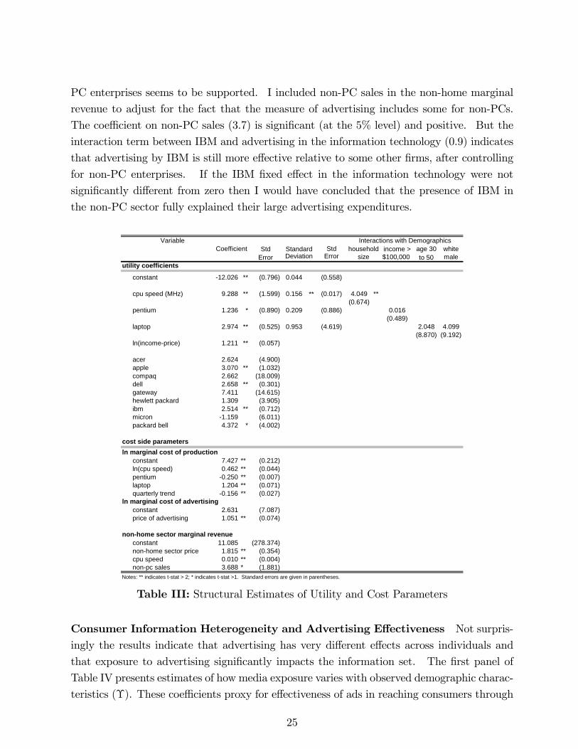
PC enterprises seems to be supported. I included non-PC sales in the non-home marginal

revenue to adjust for the fact that the measure of advertising includes some for non-PCs.

The coe¢ cient on non-PC sales (3.7) is signi�cant (at the 5% level) and positive. But the

interaction term between IBM and advertising in the information technology (0.9) indicates

that advertising by IBM is still more e¤ective relative to some other �rms, after controlling

for non-PC enterprises. If the IBM �xed e¤ect in the information technology were not

signi�cantly di¤erent from zero then I would have concluded that the presence of IBM in

the non-PC sector fully explained their large advertising expenditures.

Variable Interactions with DemographicsStd Standard Std household income > age 30 white

Error Deviation Error $100,000 to 50 maleutility coefficients

constant ­12.026 ** (0.796) 0.044 (0.558)

cpu speed (MHz) 9.288 ** (1.599) 0.156 ** (0.017) 4.049 **(0.674)

pentium 1.236 * (0.890) 0.209 (0.886) 0.016(0.489)

laptop 2.974 ** (0.525) 0.953 (4.619) 2.048 4.099(8.870) (9.192)

ln(income­price) 1.211 ** (0.057)

acer 2.624 (4.900)apple 3.070 ** (1.032)compaq 2.662   (18.009)dell 2.658 ** (0.301)gateway 7.411   (14.615)hewlett packard 1.309 (3.905)ibm 2.514 ** (0.712)micron ­1.159 (6.011)packard bell 4.372 * (4.002)

cost side parametersln marginal cost of production

constant 7.427 ** (0.212)ln(cpu speed) 0.462 ** (0.044)pentium ­0.250 ** (0.007)laptop 1.204 ** (0.071)quarterly trend ­0.156 ** (0.027)

ln marginal cost of advertisingconstant 2.631 (7.087)price of advertising 1.051 ** (0.074)

non­home sector marginal revenueconstant 11.085 (278.374)non­home sector price 1.815 ** (0.354)cpu speed 0.010 ** (0.004)non­pc sales 3.688 * (1.881)

Notes: ** indicates t­stat > 2; * indicates t­stat >1.  Standard errors are given in parentheses.

sizeCoefficient

Table III: Structural Estimates of Utility and Cost Parameters

Consumer Information Heterogeneity and Advertising E¤ectiveness Not surpris-

ingly the results indicate that advertising has very di¤erent e¤ects across individuals and

that exposure to advertising signi�cantly impacts the information set. The �rst panel of

Table IV presents estimates of how media exposure varies with observed demographic charac-

teristics (�). These coe¢ cients proxy for e¤ectiveness of ads in reaching consumers through

25

various media. The results indicate magazines are most e¤ective at reaching high income

individuals where the e¤ectiveness is increasing in household size. Newspapers are most ef-

fective at reaching high income, married individuals who are above the age of 30. Although

newspaper advertising is less likely to reach a family the larger is their household (�0:04).Hence, newspaper advertising targeted at large households would not be e¤ective in increas-

ing the probability of being informed for this particular cohort. Perhaps not surprisingly,

TV advertising is the most e¤ective medium for reaching low income households. Television

advertising is also e¤ective at reaching married individuals over 50, although not as e¤ective

as newspaper. Interestingly most advertising in the PC industry is in magazines, suggesting

PC �rms target high income households.

Coefficient estimates for interactions with mediaMagazine (mag) Newspaper (np) Television (tv) Radio

Variable Std. Error Std. Error Std. Error Std. Error Std. Errorconsumer information heterogeneity coefficientsmedia and demographic interactions (Υ)

constant ­1.032 ** (0.040) ­0.973 ** (0.040) ­1.032 ** (0.041) ­1.000 ** (0.043)30to50 (=1 if 30<age<50 ­0.042 * (0.025) 0.207 ** (0.025) 0.019 (0.025) ­0.030 * (0.025)50plus (=1 if age>50) 0.005 (0.025) 0.541 ** (0.025) 0.193 ** (0.025) ­0.245 ** (0.025)married (=1 if married) ­0.022 * (0.018) 0.187 ** (0.018) 0.075 ** (0.018) ­0.011 (0.018)hh size (household size) 0.040 ** (0.006) ­0.038 ** (0.006) 0.018 ** (0.006) 0.012 * (0.006)inclow (=1 if income<$60,000) ­0.194 ** (0.021) ­0.251 ** (0.021) 0.114 ** (0.021) ­0.117 ** (0.022)inchigh (=1 if income>$100,000) 0.153 ** (0.029) 0.127 ** (0.028) ­0.025 (0.030) 0.069 ** (0.030)malewh (=1 if male and white) ­0.078 ** (0.018) 0.002 (0.018) ­0.019 * (0.018) 0.006 (0.018)eduhs (=1 if highest edu 12 years) ­0.102 ** (0.026) ­0.338 ** (0.026) 0.296 ** (0.027) 0.076 ** (0.027)eduad (=1 if highest edu 1­3 college) 0.032 * (0.028) ­0.166 ** (0.027) 0.278 ** (0.028) 0.115 ** (0.029)edubs (=1 if highest edu college grad) ­0.024 (0.025) ­0.063 ** (0.024) 0.145 ** (0.025) 0.081 ** (0.026)edusp (education if <11) ­0.028 ** (0.003) ­0.069 ** (0.003) 0.034 ** (0.003) ­0.014 ** (0.003)

advertising media exposure (ζ)media exposure * advertising 0.948 ** (0.059)

demographics (λ)constant 0.104 ** (0.004)high school graduate 0.834 ** (0.028)income < $60,000 0.687 ** (0.009)income > $100,000 0.139 (0.318)

information technology coefficients common across consumersage of pc 0.159 ** (0.005)media advertising (φ,ρ)

npand mag advertising 0.720 * (0.488)tv advertising 1.078 ** (0.418)(np and mag advertising)2 ­0.013 (0.014)(tv advertising)2 ­0.049 ** (0.004)

firm total advertising (Ψ)acer 0.520 (0.042)apple 0.163 (0.790)compaq 0.504 ** (0.077)dell 0.497 * (0.460)gateway 0.918 ** (0.065)hewlett packard 0.199 (11.750)ibm 0.926 ** (0.184)micron 0.029 (5.832)packard bell 0.231 * (0.149)

group advertising (π)group advertising 0.891 ** (0.007)(group advertising)2 0.104 ** (0.011)

Notes: ** indicates t­stat > 2; * indicates t­stat >1.  Unless units are specified variable is a dummy.

CoefficientCoefficient Coefficient Coefficient Coefficient

Table IV: Structural Estimates of Information Technology Parameters

The results con�rm that variation in ad media exposure across households is an important

source of consumer heterogeneity. The variation in ad exposure translates into variation

in information sets as evidenced by the positive and highly signi�cant estimate for &. The

26

estimates highlight the importance of considering the di¤erential e¤ects of advertising both

across households and across media. Most of the literature does not incorporate consumer

information heterogeneity, which has implications for markups as discussed shortly.

Parameter estimates of e� suggest other means of information provision, such as word-of-mouth or experience, play a role in informing certain types of consumers. The coe¢ cient on

income less than $60,000 (0:69) indicates these individuals are likely to be informed about

41% of the products without seeing an ad. Whereas having a high income is not signi�cantly

di¤erent from having a middle income, in terms of being informed without seeing an ad. This

could arise because low income individuals are likely to have lower opportunity costs and

thus more time to search for information. In addition, the probability of being informed

without seeing any advertising is higher for high-school grads relative to non-graduates.

The lower panel presents estimates of the parameters that are the same across households

(the j parameters). Consumers are signi�cantly more likely to know a PC the longer it has

been on the market (0:16): This is intuitive, for the longer it has been on the market the

more opportunity consumers have had to learn of it by word-of-mouth or through advertising.

There are decreasing returns to advertising in the TV (�0:05) and newspapers and magazines(�0:01) media, but they are decreasing at a faster rate for TV. Estimates of �rm �xed

e¤ects interacted with total advertising () indicate that some �rms are more e¤ective at

informing consumers through advertising. Most notably ads by Compaq, Dell, Gateway,

IBM and Packard Bell are signi�cantly more e¤ective, which could be due to di¤erences in

advertising techniques across �rms.

Some products are advertised in groups while others are advertised individually. The

coe¢ cient estimates on group advertising (�1) and group advertising squared (�2) are given

in the last rows of Table IV. These (unrestricted) estimates predict that we will observe

both group and product speci�c advertising, which is supported by the data. There are

economies of scope in group advertising (0:1). The estimates imply that if average group

ad expenditures (ad) for a particular product group are above a threshold level of $1.05

million per quarter45 (either the expenditures for a group are high or the groups are small)

the �rm will �nd it worthwhile to engage in group advertising to capitalize on the economies

of scope. To put this into context, in the �rst quarter of 1998 Apple�s advertising strategy

involved 17 group advertisements. The estimates suggest we would observe 17 group ads

only if Apple�s home sector advertising budget was at least $18 million. Apple spent over

$180 million in advertising in 1998 and more than $20 million in the �rst quarter �consistent

with the model�s prediction.

45The ad threshold is (1� �1)=�2: If there is only one product in the group I restrict �1 = 1 and �2 = 0.

27

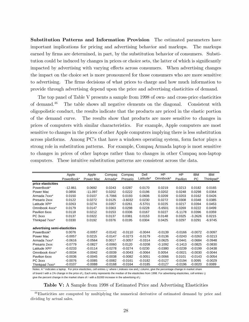
Substitution Patterns and Information Provision The estimated parameters have

important implications for pricing and advertising behavior and markups. The markups

earned by �rms are determined, in part, by the substitution behavior of consumers. Substi-

tution could be induced by changes in prices or choice sets, the latter of which is signi�cantly

impacted by advertising with varying e¤ects across consumers. When advertising changes

the impact on the choice set is more pronounced for those consumers who are more sensitive

to advertising. The �rms decisions of what prices to charge and how much information to

provide through advertising depend upon the price and advertising elasticities of demand.

The top panel of Table V presents a sample from 1998 of own- and cross-price elasticities

of demand.46 The table shows all negative elements on the diagonal. Consistent with

oligopolistic conduct, the results indicate that the products are priced in the elastic portion

of the demand curve. The results show that products are more sensitive to changes in

prices of computers with similar characteristics. For example, Apple computers are most

sensitive to changes in the prices of other Apple computers implying there is less substitution

across platforms. Among PC�s that have a windows operating system, form factor plays a

strong role in substitution patterns. For example, Compaq Armada laptop is most sensitive

to changes in prices of other laptops rather than to changes in other Compaq non-laptop

computers. These intuitive substitution patterns are consistent across the data.

Apple Apple Compaq Compaq Dell HP HP IBM IBMPowerBook* Power Mac Armada* Presario Latitude* Omnibook* Pavilion PC Thinkpad*

price elasticitiesPowerBook* ­12.861 0.0692 0.0243 0.0287 0.0170 0.0219 0.0213 0.0182 0.0165Power Mac 0.0856 ­11.097 0.0202 0.0222 0.0196 0.0202 0.0248 0.0298 0.0364Armada 7xxx* 0.0150 0.0107 ­5.7066 0.0193 0.0606 0.0209 0.0203 0.0162 0.0426Presario 2xxx 0.0122 0.0272 0.0125 ­3.6032 0.0230 0.0272 0.0308 0.0348 0.0385Latitude XPI* 0.0263 0.0274 0.0357 0.0261 ­5.5701 0.0225 0.0217 0.0394 0.0453Omnibook 4xxx* 0.0179 0.0147 0.0363 0.0298 0.0228 ­5.6501 0.0269 0.0222 0.0499Pavilion 6xxx 0.0118 0.0212 0.0153 0.0336 0.0167 0.0227 ­5.1178 0.0396 0.0359PC 3xxx 0.0137 0.0322 0.0137 0.0381 0.0153 0.0148 0.0325 ­3.2626 0.0215Thinkpad 7xxx* 0.0330 0.0192 0.0376 0.0195 0.0304 0.0425 0.0297 0.0291 ­6.9745

advertising semi­elasticitiesPowerBook* 0.0076 ­0.0057 ­0.0142 ­0.0110 ­0.0044 ­0.0139 ­0.0166 ­0.0072 ­0.0097Power Mac ­0.0057 0.0215 ­0.0147 ­0.0273 ­0.0179 ­0.0136 ­0.0243 ­0.0263 ­0.0213Armada 7xxx* ­0.0616 ­0.0564 0.0017 ­0.0057 ­0.0314 ­0.0625 ­0.0441 ­0.0684 ­0.0948Presario 2xxx ­0.0779 ­0.0827 ­0.0060 0.0120 ­0.0208 ­0.1092 ­0.1413 ­0.0825 ­0.0830Latitude XPI* ­0.0233 ­0.0114 ­0.0278 ­0.0274 0.0230 ­0.0380 ­0.0239 ­0.0199 ­0.0438Omnibook 4xxx* ­0.0034 ­0.0042 ­0.0039 ­0.0043 ­0.0064 0.0054 ­0.0021 ­0.0030 ­0.0044Pavilion 6xxx ­0.0036 ­0.0045 ­0.0038 ­0.0082 ­0.0051 ­0.0066 0.0101 ­0.0143 ­0.0054PC 3xxx ­0.0076 ­0.0085 ­0.0082 ­0.0161 ­0.0182 ­0.0127 ­0.0194 0.0095 ­0.0029Thinkpad 7xxx* ­0.0107 ­0.0088 ­0.0168 ­0.0164 ­0.0185 ­0.0127 ­0.0196 ­0.0020 0.0089Notes: A * indicates a laptop.  For price elasticities, cell entries i,j where i ,indexes row and j  column, give the percentage change in market shareof brand I with a 1% change in the price of j. Each entry represents the median of the elasticities from 1998. For advertising elasticities, cell entries i,jgive the percent change in the market share of i  with a $1000 increase in the advertising of j.

Table V: A Sample from 1998 of Estimated Price and Advertising Elasticities

46Elasticities are computed by multiplying the numerical derivative of estimated demand by price anddividing by actual sales.

28

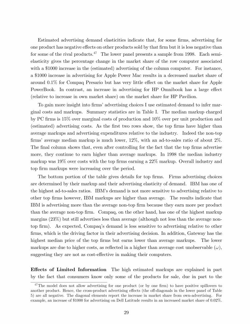
Estimated advertising demand elasticities indicate that, for some �rms, advertising for

one product has negative e¤ects on other products sold by that �rm but it is less negative than

for some of the rival products.47 The lower panel presents a sample from 1998. Each semi-

elasticity gives the percentage change in the market share of the row computer associated

with a $1000 increase in the (estimated) advertising of the column computer. For instance,

a $1000 increase in advertising for Apple Power Mac results in a decreased market share of

around 0.1% for Compaq Presario but has very little e¤ect on the market share for Apple

PowerBook. In contrast, an increase in advertising for HP Omnibook has a large e¤ect

(relative to increase in own market share) on the market share for HP Pavilion.

To gain more insight into �rms�advertising choices I use estimated demand to infer mar-

ginal costs and markups. Summary statistics are in Table I. The median markup charged

by PC �rms is 15% over marginal costs of production and 10% over per unit production and

(estimated) advertising costs. As the �rst two rows show, the top �rms have higher than

average markups and advertising expenditures relative to the industry. Indeed the non-top

�rms�average median markup is much lower, 12%, with an ad-to-sales ratio of about 2%.

The �nal column shows that, even after controlling for the fact that the top �rms advertise

more, they continue to earn higher than average markups. In 1998 the median industry

markup was 19% over costs with the top �rms earning a 22% markup. Overall industry and

top �rm markups were increasing over the period.

The bottom portion of the table gives details for top �rms. Firms advertising choices

are determined by their markup and their advertising elasticity of demand. IBM has one of

the highest ad-to-sales ratios. IBM�s demand is not more sensitive to advertising relative to

other top �rms however, IBM markups are higher than average. The results indicate that

IBM is advertising more than the average non-top �rm because they earn more per product

than the average non-top �rm. Compaq, on the other hand, has one of the highest markup

margins (23%) but still advertises less than average (although not less than the average non-

top �rm). As expected, Compaq�s demand is less sensitive to advertising relative to other

�rms, which is the driving factor in their advertising decision. In addition, Gateway has the

highest median price of the top �rms but earns lower than average markups. The lower

markups are due to higher costs, as re�ected in a higher than average cost unobservable (!),

suggesting they are not as cost-e¤ective in making their computers.

E¤ects of Limited Information The high estimated markups are explained in part

by the fact that consumers know only some of the products for sale, due in part to the

47The model does not allow advertising for one product (or by one �rm) to have positive spillovers toanother product. Hence, the cross-product advertising e¤ects (the o¤-diagonals in the lower panel of Table5) are all negative. The diagonal elements report the increase in market share from own-advertising. Forexample, an increase of $1000 for advertising on Dell Latitude results in an increased market share of 0.02%.

29

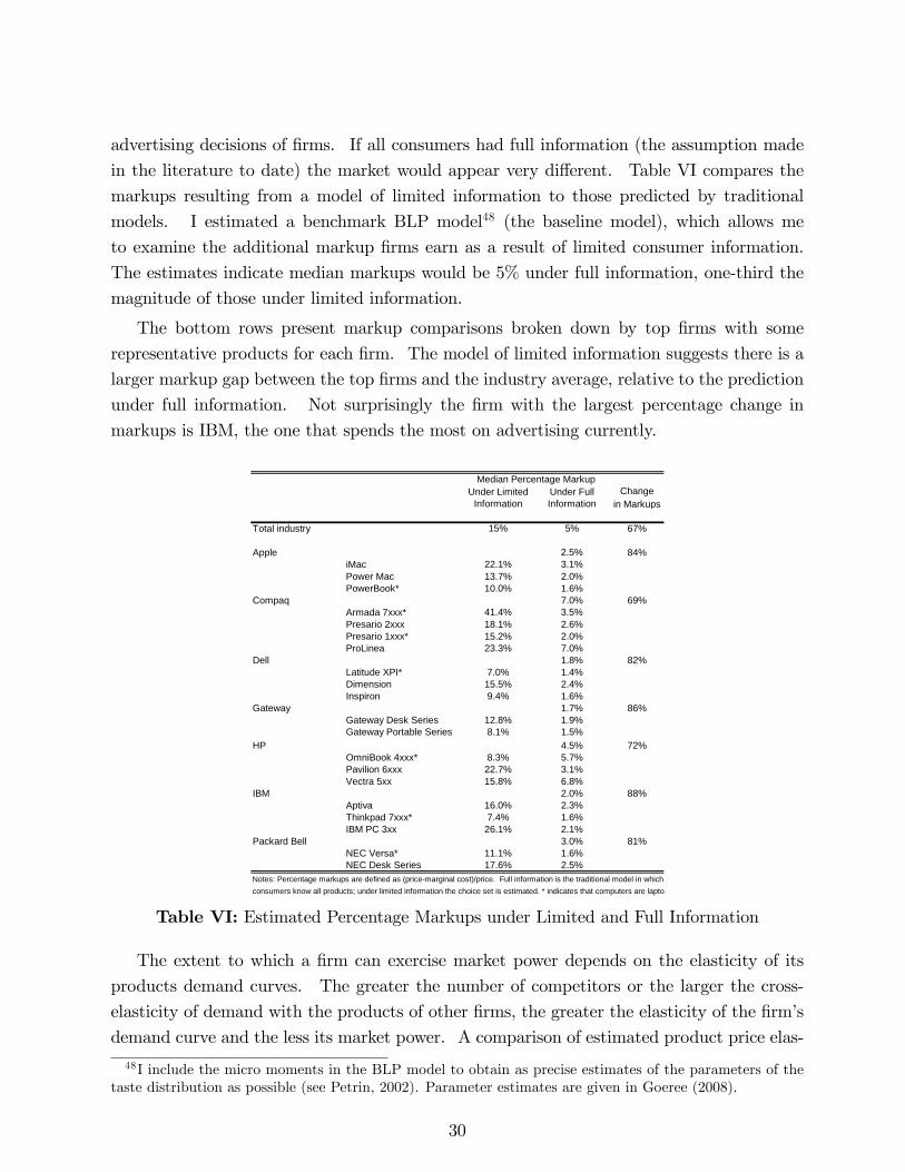
advertising decisions of �rms. If all consumers had full information (the assumption made

in the literature to date) the market would appear very di¤erent. Table VI compares the

markups resulting from a model of limited information to those predicted by traditional

models. I estimated a benchmark BLP model48 (the baseline model), which allows me

to examine the additional markup �rms earn as a result of limited consumer information.

The estimates indicate median markups would be 5% under full information, one-third the

magnitude of those under limited information.

The bottom rows present markup comparisons broken down by top �rms with some

representative products for each �rm. The model of limited information suggests there is a

larger markup gap between the top �rms and the industry average, relative to the prediction

under full information. Not surprisingly the �rm with the largest percentage change in

markups is IBM, the one that spends the most on advertising currently.

Median Percentage MarkupUnder Limited Under Full Change

Information Information in Markups

Total industry 15% 5% 67%

Apple 2.5% 84%iMac 22.1% 3.1%Power Mac 13.7% 2.0%PowerBook* 10.0% 1.6%

Compaq 7.0% 69%Armada 7xxx* 41.4% 3.5%Presario 2xxx 18.1% 2.6%Presario 1xxx* 15.2% 2.0%ProLinea 23.3% 7.0%

Dell 1.8% 82%Latitude XPI* 7.0% 1.4%Dimension 15.5% 2.4%Inspiron 9.4% 1.6%

Gateway 1.7% 86%Gateway Desk Series 12.8% 1.9%Gateway Portable Series 8.1% 1.5%

HP 4.5% 72%OmniBook 4xxx* 8.3% 5.7%Pavilion 6xxx 22.7% 3.1%Vectra 5xx 15.8% 6.8%

IBM 2.0% 88%Aptiva 16.0% 2.3%Thinkpad 7xxx* 7.4% 1.6%IBM PC 3xx 26.1% 2.1%

Packard Bell 3.0% 81%NEC Versa* 11.1% 1.6%NEC Desk Series 17.6% 2.5%

Notes: Percentage markups are defined as (price­marginal cost)/price.  Full information is the traditional model in whichconsumers know all products; under limited information the choice set is estimated. * indicates that computers are laptops

Table VI: Estimated Percentage Markups under Limited and Full Information

The extent to which a �rm can exercise market power depends on the elasticity of its

products demand curves. The greater the number of competitors or the larger the cross-

elasticity of demand with the products of other �rms, the greater the elasticity of the �rm�s

demand curve and the less its market power. A comparison of estimated product price elas-

48I include the micro moments in the BLP model to obtain as precise estimates of the parameters of thetaste distribution as possible (see Petrin, 2002). Parameter estimates are given in Goeree (2008).

30

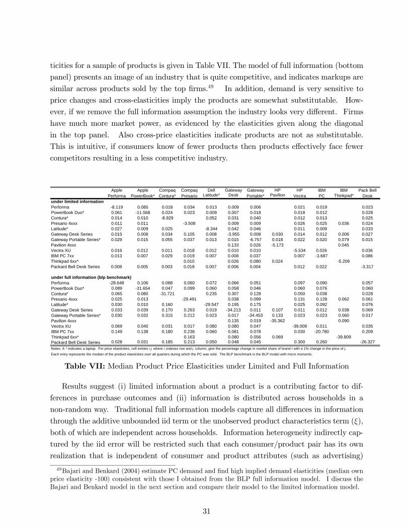
ticities for a sample of products is given in Table VII. The model of full information (bottom

panel) presents an image of an industry that is quite competitive, and indicates markups are

similar across products sold by the top �rms.49 In addition, demand is very sensitive to

price changes and cross-elasticities imply the products are somewhat substitutable. How-

ever, if we remove the full information assumption the industry looks very di¤erent. Firms

have much more market power, as evidenced by the elasticities given along the diagonal

in the top panel. Also cross-price elasticities indicate products are not as substitutable.

This is intuitive, if consumers know of fewer products then products e¤ectively face fewer

competitors resulting in a less competitive industry.

Apple Apple Compaq Compaq Dell Gateway Gateway HP HP IBM IBM Pack BellPerforma PowerBook* Contura* Presario Latitude* Desk Portable* Pavilion Vectra PC Thinkpad* Desk

under limited informationPerforma ­8.119 0.085 0.018 0.034 0.013 0.009 0.006 0.021 0.019 0.023PowerBook Duo* 0.061 ­11.568 0.024 0.023 0.009 0.007 0.018 0.018 0.012 0.028Contura* 0.014 0.010 ­8.929 0.052 0.031 0.040 0.012 0.013 0.025Presario 4xxx 0.011 0.011 ­3.508 0.009 0.009 0.026 0.025 0.036 0.024Latitude* 0.027 0.009 0.025 ­8.344 0.042 0.046 0.011 0.009 0.033Gateway Desk Series 0.015 0.008 0.034 0.105 0.008 ­3.955 0.008 0.030 0.014 0.012 0.006 0.027Gateway Portable Series* 0.029 0.015 0.055 0.037 0.013 0.015 ­6.757 0.018 0.022 0.020 0.079 0.015Pavilion 4xxx 0.133 0.026 ­5.173 0.045Vectra XU 0.016 0.012 0.011 0.018 0.012 0.010 0.010 ­5.534 0.026 0.036IBM PC 7xx 0.013 0.007 0.029 0.019 0.007 0.008 0.037 0.007 ­3.687 0.086Thinkpad 6xx* 0.010 0.026 0.080 0.024 ­5.209Packard Bell Desk Series 0.008 0.005 0.003 0.018 0.007 0.006 0.004 0.012 0.022 ­3.317

under full information (blp benchmark)Performa ­28.648 0.106 0.088 0.060 0.072 0.066 0.051 0.097 0.090 0.057PowerBook Duo* 0.089 ­31.654 0.047 0.099 0.060 0.058 0.046 0.060 0.076 0.060Contura* 0.065 0.080 ­31.721 0.235 0.307 0.128 0.050 0.038 0.028Presario 4xxx 0.025 0.013 ­29.491 0.038 0.099 0.131 0.128 0.062 0.061Latitude* 0.030 0.010 0.160 ­29.547 0.195 0.175 0.025 0.092 0.076Gateway Desk Series 0.033 0.039 0.170 0.263 0.019 ­34.213 0.011 0.107 0.011 0.012 0.038 0.069Gateway Portable Series* 0.030 0.032 0.315 0.212 0.023 0.017 ­34.453 0.133 0.023 0.023 0.060 0.017Pavilion 4xxx 0.135 0.019 ­35.362 0.090Vectra XU 0.069 0.040 0.031 0.017 0.080 0.080 0.047 ­39.009 0.011 0.035IBM PC 7xx 0.149 0.138 0.180 0.236 0.060 0.081 0.078 0.030 ­20.780 0.209Thinkpad 6xx* 0.163 0.080 0.056 0.069 ­39.809Packard Bell Desk Series 0.028 0.031 0.185 0.213 0.050 0.048 0.045 0.300 0.260 ­26.327Notes: A * indicates a laptop.  For price elasticities, cell entries i,j where i ,indexes row and j  column, give the percentage change in market share of brand I with a 1% change in the price of j.Each entry represents the median of the product elasticities over all quarters during which the PC was sold.  The BLP benchmark is the BLP model with micro moments.

Table VII: Median Product Price Elasticities under Limited and Full Information

Results suggest (i) limited information about a product is a contributing factor to dif-

ferences in purchase outcomes and (ii) information is distributed across households in a

non-random way. Traditional full information models capture all di¤erences in information

through the additive unbounded iid term or the unobserved product characteristics term (�),

both of which are independent across households. Information heterogeneity indirectly cap-

tured by the iid error will be restricted such that each consumer/product pair has its own

realization that is independent of consumer and product attributes (such as advertising)

49Bajari and Benkard (2004) estimate PC demand and �nd high implied demand elasticities (median ownprice elasticity -100) consistent with those I obtained from the BLP full information model. I discuss theBajari and Benkard model in the next section and compare their model to the limited information model.

31

and of all other consumer/product pairs. This doesn�t permit correlation in information

across consumers, nor does it permit informational advantages to depend on consumer and

product observables. Alternatively, information heterogeneity can be indirectly captured

via unobserved product characteristics. In the model of limited information, a product with

little advertising is unlikely to be in many consumer�s choice sets and will have a low market

share. In the BLP model, a small market share could be explained by a low value for �j:50

Again, the unobserved term is independent of consumer attributes. Not explicitly allowing

for informational asymmetries is particularly restrictive in rapidly changing markets where

consumers are likely to have limited information, and hence where heterogeneity in the dis-

tribution of information across consumers and products explains (perhaps a signi�cant) part

of the variation in sales across products.

The results indicate that relying on an additive unbounded iid error term or unobserved

product characteristics to explain di¤erences in information across consumer-product pairs

can generate inconsistent estimates of product speci�c demand curves that are biased towards

being too elastic. Consider as an example a market that consists of three products each

produced by a di¤erent �rm. These products have identical characteristics, but the �rms

are each monopolies due to limited consumer information. That is, there are three groups

of consumers where each group knows only one product. In this world, each of the three

�rms would earn monopoly markups. Let�s consider how the full and limited information

models would address the data generated from such a world.

First, assume the consumers are identical. In the data we would observe identical individ-

uals purchasing di¤erent products with identical observed characteristics. The model would

need to make the products di¤er somehow to match the data. Traditional models would rely

on the iid term to explain the observed purchase patterns. (The model couldn�t use di¤erent

� to match the data since all consumers would buy the product with the highest �:) Would

this result change if consumers were heterogenous, that is could the model explain di¤erent

purchases through di¤erent consumer tastes? No, because observed product characteristics

are the same (i.e. a consumer with a large taste for CPU speed has to choose among three

products with identical CPU speed, that are also identical in every other observable respect).

There are two points here (i) the iid terms would allow the model to match the purchase

patterns but would use random consumer-product variation to do so (ii) the estimated elas-

ticities would be more elastic than the true elasticities. Estimated markups would be much

lower than true markups.

The limited information framework could explain di¤erences in choices among otherwise

identical products through di¤erences in consumer information across products. First, in the

case of no advertising, the model permits information heterogeneity due to di¤erences in con-

50I thank an anonymous referee for this point.

32

sumer attributes. Second, household information heterogeneity could arise if �rms advertise

products using di¤erent media where certain media are more e¤ective at informing certain

types of consumers. The limited information model allows consumers to be non-randomly

di¤erentially informed, which may explain di¤erences in purchase patterns observed in the

data. There are two points here (i) the limited information model matches purchase patterns

using non-random information heterogeneity across consumers and products (relying less on

the iid term) (ii) the estimated elasticities would be more inelastic than the traditional elas-

ticities. In this example, the markups estimated from the limited information model would

be higher relative to those obtained under traditional models.

Consider another example. The market again consists of three products with identical

observed characteristics, but product one has a low market share relative to the others.

Again, for the sake of illustration, assume product one is a high quality product where the

unequal distribution of market shares is due to limited information: few consumers know

product one. The BLP model can match the data through one of two ways (i) through

the iid error term (ii) through unobserved product characteristics (�): Since mean utility is

chosen to match market shares, the model will force product one�s mean utility to be lower

through a low value of �. This has the implication that consumers are more sensitive to

price changes in product one, ceteris paribus, since their mean utility is lower. However, in

truth product one is a high quality product, and hence should have a high � value. The

limited information model would allow for the following: few consumers are informed about

the existence of product one (perhaps due to low advertising for the product), implying it

has a low market share. High quality implies a high value of � resulting in higher utility

for consumers who know the product, ceteris paribus, resulting in more inelastic demand

among fewer consumers. The limited information model would predict that product one

would have higher markups than those predicted by traditional models.

This is best illustrated by examining the di¤erences in the value of the unobserved product

characteristics terms when the parameters are estimated via BLP full information versus

limited information models. Apple�s PowerBook G3 was introduced in November 1997 and

was designed to use a high speed �backside�cache which could interact with the processor

at much faster speeds than a standard L2 cache (which was restricted by the motherboard

speed). At the time, the PowerBook G3 was considered the fastest notebook in the world. It

received very favorable reviews for its speed, weight, size, design, and overall performance.51

The PowerBook G3 had a very small share of the market, both because Apple�s market share

was low during this period (around 6%) and also because the PowerBook G3 was only on

the market for 5 months. To match the low market shares, the BLP model generates a low

value of � (relative to other products in the quarter). In contrast, the limited information

51apple-history.com;pcworld.com/article/id,11954/article.html; epinions.com; consumerreports.com

33

model generates a low average value for �, but a signi�cantly higher � value than in the BLP

model. The anecdotal evidence seems to support the limited information results: there are

few consumers who know the PowerBook G3, but among the informed subset mean utility

is increased from buying it, ceteris paribus. This suggests Apple could earn a high markup

on the PowerBook G3 from the subset of consumers who know it. Indeed, the estimated

limited information markups for PowerBook G3 are on the order of 11%, while the BLP

estimates suggest this is a product with low markups (around 1%). The results suggest that

traditional models, which rule out non-random informational asymmetries across households

and products a priori, yield inconsistent estimates for product speci�c elasticities that are

biased towards being too elastic.52

8. Sensitivity Analysis

I examine the robustness of the limited information model by conducting goodness-of-�t tests.

First, I tested whether all the moments were satis�ed. The objective function is a Wald

statistic distributed chi-squared with degrees of freedom equal to the number of moment

restrictions less the number of parameters. This test is conditional on all assumptions of the

model and tests the overidentifying moment restrictions together with all functional form

and distributional assumptions. The test is stringent and generally rejects for large samples.

It is not surprising then, given the large sample size and stylized nature of the model, that

the model is rejected by the data.

Second, I conducted goodness-of-�t tests focused on various aspects of the model. I

partitioned the region in which the response variables (and in some cases covariates) lie into

disjoint cells. I calculated the quadratic form based on the di¤erence between the observed

number of outcomes in each cell and the expected number (given the observed covariates). If

the model is correct, the normalized quadratic form converges in distribution to a chi-square

random variable as the sample size increases.53

Formal tests were not able to reject the null that predicted values for market shares are

the same as the observed values.54 I also constructed test statistics based on the average

value of shares that fall into speci�ed cells. Again, the test statistic is below the 10%

level of signi�cance critical value: the null hypothesis is not rejected. Controlling for

product attributes, the model does a good job of predicting average market shares across

52See Goeree (2002, 2008) for details concerning why full information and limited information models will(most likely) result in di¤erent estimates for price elasticities of demand.53These tests are based on those presented in Andrews(1988). The predetermined number of cells are

centered at the mean of the response variable with a width proportional to its standard deviation.54The test statistic is chi-squared with 7 degrees of freedom. The realized value (4.7) is below the 10%

level critical value (12). The model �ts well, but misses more among lower market share products.

34

cells. However the model tends to miss more among non-Pentiums.

Third, I compared the limited information model (hereafter LIM) to three alternatives.

The �rst is the BLP model (with micro moments). The second is a full information model

where advertising a¤ects the utility function directly. I refer to this model as the uninforma-

tive model (hereafter UN). The third is a modi�cation of the BLP model proposed by Bajari

and Benkard (2005, hereafter BB). They estimate PC demand and �nd high estimated

own-price elasticities. They (independently) attribute their unrealistically high estimates

to the full information assumption. They estimate a modi�ed BLP model limited to those

products with large market shares. The intuition being consumers are more likely to know

these products since it is easier to obtain information on them.55

I would prefer to be able to test the relative �t of the models parametrically. Un-

fortunately a formal test of non-nested hypotheses (Vuong, 1989) would require additional

assumptions on the distribution of the errors. While the data suggest no natural assumptions

for the error distributions I present analysis that highlights the strengths and weaknesses of

the �t of LIM relative to other models. For instance, both LIM and UN predict a threshold

level of average group ad expenditures (above which products will be advertised in groups

and below which they will be advertised individually). We should never observe group

(product speci�c) expenditures below (above) this level. The LIM and UN models predict

di¤erent threshold levels. These predictions are presented in the second panel of Table VIII.

The LIM model misses about 3% of the time, while UN misses more than twice as much, 8%.

Most of the misses for both models are among Apple products (2.4% for LIM and 8% for

UN), while both models�predictions match the data for HP and Packard Bell. In addition,

both models miss more among TV advertisements (1.5% for LIM and 5.5% for UN). The fact

that UN �ts worse in this dimension is not surprising since UN predicts a higher threshold

level (so we expect to observe a larger percentage of group expenditures below the predicted

threshold). It is surprising that LIM does no worse than UN regarding the proportion of

product speci�c expenditures above the predicted threshold. Both models miss less than 1%

on average, with all the misses coming among Apple and Compaq products. This anecdotal

evidence suggests, at the very least, that the LIM model �ts no worse than the UN model.

Another dimension along which the models can be compared regards the role of unob-

served product attributes. In all models mean utility is chosen such that predicted shares

match observed shares. While there is no explicit role for advertising in the BLP model or

BB modi�cation, one can interpret the unobserved product heterogeneity terms ( �j) as con-

taining product advertising.56 Using the parameter estimates from the respective models, I

55The parameter estimates for the alternative models can be found in Goeree (2008).56In the LIM model, a product with little advertising is unlikely to be in many consumer�s choice sets and

will have a low market share. In the BLP and BB models, a small market share would be explained by a

35

restricted �j to zero and recalculated the predicted market shares. These �pseudo�predicted

shares are presented in the �rst panel of Table VIII. These provide insight into the impor-

tance of unobserved product attributes in each model as well as indicate how well the model

�ts market shares based solely on observables and the form of the model.

Prediction for different modelsObserved Limited Full Information Full Information Large Market

Information Uninformative No Advertising Shares OnlyResponse Variable Advertising BLP Bajari/Benkard

average annual percent unit market sharesApple 6.45% 8.87% 8.96% 5.15% 6.54% **Compaq 16.17% 17.75% * 17.98% 19.74% 22.16%Gateway 10.76% 11.32% ** 10.99% ** 13.07% 13.34%HP 6.53% 6.86% ** 5.99% * 1.98% 7.85%IBM 7.60% 8.51% * 8.59% 9.38% 8.10% *Packard Bell 22.61% 20.37% * 24.34% * 27.41% 27.00%

mean industry elasticity 4.39% 4.41% 4.41% 4.38%

group and product­specific advertisingPredicted threshold value ($millions) 1.05 1.66 not not

applicable applicablepercent group expenditures below predicted threshold valueAll products 2.7% 8.2%

Apple 2.4% 8.2%Compaq 1.4% 4.4%Gateway 1.1% 2.6%HP 0.0% 0.0%IBM 1.1% 3.8%Packard Bell 0.0% 0.0%

Newspaper 0.0% 0.8%Magazine 0.1% 0.9%Television 1.5% 5.5%Radio 0.9% 0.9%

percent product­specific expenditures above predicted threshold valueAll products 0.8% 0.8%

Apple 0.9% 0.9%Compaq 0.9% 0.9%Gateway 0.0% 0.0%HP 0.0% 0.0%IBM 0.0% 0.0%Packard Bell 0.0% 0.0%

Newspaper 0.0% 0.0%Magazine 0.8% 0.8%Television 0.1% 0.1%Radio 0.8% 0.8%

Notes: Predicted market shares are evaluated at parameter estimates with unobserved product attributes restricted to zero. ** indicates thatpredicted values within 5% of the observed value * within 10% of the true value.  Predicted group advertising expenditures threshold valuein millions. Advertising expenditures are computed using equation (1) evalulated at the optimal parameter values.   Firm percentages arecalculated as percent of product/medium advertising by that firm.  The BLP model includes micro moments.  The Bajari/Benkard (BB)model includes only those products which sold more than 5000 units.

Table VIII: Goodness of Fit

The BLP model�s predicted pseudo shares do not come within 10% of the observed market

shares for any of the top �rms (second to last column). The BB modi�cation (last column)

�ts the market shares of the top �rms better than the BLP model, the Apple shares are

within 5% of the observed shares and IBM within 10%. This is not surprising since BB

low value for �j :

36

restricts estimation to the larger �rms. Both BLP and BB provide a worse �t than the

models in which advertising plays an explicit role. Again, this is not a surprise as the �jplay a larger role in the BLP and BB model relative to the advertising models. The LIM

model �ts the market shares better than the UN model. For Gateway and HP, the pseudo

market shares are within 5% of observed shares and for Compaq, IBM, and Packard Bell,

the pseudo shares are within 10%. The UN model comes within 5% of the observed market

shares for Gateway and within 10% for HP and Packard Bell. Neither model predicts Apple

market shares within 10%. This is perhaps not so surprising given that the �rm for which

the advertising predictions miss the most is Apple. These results suggest the model of

limited information does a good job of predicting advertising and market shares in the PC

industry, relative to models in which consumers are assumed to be aware of all products.

While the alternative models present di¤erent pictures of product elasticities, they are

consistent in their predictions of industry elasticities. For all models, I simulate a 1% increase

in the price of all (inside) goods and calculate the percentage change in total home market

share. Mean industry elasticities are given in the second panel. Industry demand is more

inelastic, an intuitive result given the relative scarcity of products which are substitutable

for PCs (particularly over this time frame).

Due to the di¢ culty in obtaining ad data for some industries, a comparison of BLP and

BB may be useful. If LIM is believed to be the correct model, then the BB modi�cation

may be preferred in that it generates estimates of product demand curves that are less elastic

(relative to BLP) and closer in magnitude to those of LIM.57 However, the �j still play a

large role in BB, namely only for Apple is the reliance on the �j small enough to provide an

adequate �t of market shares based on observables. To the extent that the role (or number

of) smaller �rms is an important dimension of industry competition, the BB modi�cation

will not be preferred to other models of full information.

Recall, that LIM restricts attention to the top ten �rms plus �ve other small �rms. This

sample selection could e¤ect estimated margins in two ways. First the smaller products

not included in the sample are likely to have higher own-price elasticities and hence lower

markups (relative to similar included products). Estimated markups for the included prod-

ucts will be higher the more smaller �rms (or less-advertising intensive �rms) are excluded.

This e¤ect would be in largest for the BB modi�cation which limits the sample to large

�rms. Indeed BB found evidence of much higher markups (less elastic demand curves).

This e¤ect is less pronounced for LIM in that �ve of the �rms are small. The other e¤ect of

limiting the sample has to do with the impact on the �outside�good. The fewer products

are included among the �inside� goods (the larger is the outside good) the lower will be

57BB �nd estimated product speci�c demand elasticities ranging from -4 to -72 with a median elasticityof -11 for their modi�ed model.

37

estimated markups for the inside goods. Under full information when a product is added

to the sample that product is a competitor with every other product. The overall impact

on markups will depend upon the substitution patterns among the inside goods and the size

of the outside good. However when a product is added to the LIM model it may not be a

competitor with every other product (some consumers may not know it exists). Hence, LIM

markups will not be as sensitive to adding new �rms to the included sample as will models

of full information.

Modeling advertising as a¤ecting a consumer�s choice set requires signi�cant computation

time since the choice sets must be simulated. To test if the bene�ts of simulating choice sets

are worth the costs of increased computation time, I performed a monte-carlo experiment.

Consider a market consisting of two products and one outside good. Denote the probability

consumers are aware of a product by �j: The limited information market share is

s1 = �1(1� �2)D1

1 +D1

+ �1�2D1

1 +D1 +D2

where Dj represents exp(�j); the mean utility from product j; analogously for product 2. A

version of the market share which would not require simulating choice sets is

s�1 =�1D1

1 + �1D1

+�1D1

1 + �1D1 + �2D2

:

I calculated the values of sj and s�j for di¤erent values of � and D. The resulting value of s�j

was within 5% of the value of sj only 2% of the time. Notice also that the speci�cation for

s�j is not separately identi�able from a model in which advertising enters the utility function

directly (or a model in which advertising is included in �j). This obtains by de�ning �� =

ln(�) and D = exp(�+��): These results suggest that the more computationally demanding

LIM model cannot be replaced easily with a simpli�ed version. Secondly, advertising which

in�uences consumers�choice sets has very di¤erent e¤ects from that which shifts demand

directly through utility. That is, the standard BLP model and models in which advertising

are one of the observed product attributes are not observationally equivalent to the model

presented in this research.58

9. Conclusions

In markets characterized by rapid change, such as the PC industry, it is probable that con-

sumers know only a subset of all available products. Models estimated under the assumption58A model that includes both e¤ects of advertising, through the choice set and directly in utility, is,

theoretically, separately identi�able. However, in practice, one would like identi�cation to be driven byvariation in the data. See Ackerberg (2001, 2003) who uses micro data to estimate a model which allows forinformative and uninformative e¤ects of advertising.

38

of full information present an image of the PC industry that is quite competitive. For exam-

ple, a BLP full information model yields modest estimated median markups of 5%. When

we remove the full information assumption the industry looks very di¤erent. Indeed, esti-

mated cross-price elasticities indicate products are not as substitutable as full information

estimates suggest. I estimate a model of limited consumer information, where �rms provide

information through advertising. I �nd estimated median markups in the PC industry are

high: 19% over production costs in 1998, where the top �rms engage in higher than average

advertising and earn higher than average markups. The results suggest �rms have signi�cant

market power due in part to limited consumer information. The di¤erences in estimated

price elasticities (and implied markups) across the approaches re�ects the inconsistency in

the full information model which does not allow consumers to be di¤erentiated in terms of

information. I extend the BLP framework to permit systematic (non-random) di¤erences in

information based on consumer observables. I try to capture potential correlation in infor-

mation across consumers using di¤erences in information exposure across consumer types

based on media exposure choices. The model allows for the possibility that the imperfect

substitutability between di¤erent brands of consumer products is due to consumers�having

limited information about product o¤erings as well as to consumer-idiosyncratic brand pref-

erences. I show how to use additional data on media exposure to improve estimated price

elasticities, á la BLP, in the absence of micro ad data.

The results suggest that (i) allowing for heterogeneity in consumers�choice sets yields

more realistic estimates of substitution patterns between goods, (ii) assuming full informa-

tion may result in incorrect conclusions regarding the intensity of industry competition, and

(iii) �rms bene�t from limited consumer information. I �nd that exposure to advertising

signi�cantly impacts consumers� information sets, but that advertising has very di¤erent

informative e¤ects across individuals and across media. The estimates suggest that some

�rms are more e¤ective at informing consumers through advertising. For some �rms adver-

tising one product can have a negative e¤ect on the market share of other products sold by

that �rm, but the e¤ect is less negative than it is for most of the rivals�products. There

are economies of scope in group advertising and some �rms �nd it worthwhile to engage in

group advertising for some product lines to capitalize on the increasing returns.

Considering the implications of limited information is particularly important when ad-

dressing policy issues. In the PC industry, models estimated under the assumption that

consumers are aware of all products generate estimates of product-speci�c demand curves

that are biased towards being too elastic. The results of this paper suggest that antitrust

authorities may reach di¤erent conclusions regarding the welfare implications of mergers

depending on their assumptions regarding consumer information.59

59See Goeree (2002, 2003).

39

Appendix A. Approximations to the Optimal Instruments

To motivate the instruments discussed in section 4, it easiest to �rst consider a simplercontext. The following text borrows heavily from the Appendix to BLP (1999). The fullinformation linear model has an estimating equation of

ln(sj)� ln(s0) � �j = xj� � �pj + �j: (A.1)

The optimal instruments are E(x j z) and E(p j z) assuming � is iid. Given that x is anelement of z; E(x j z) = x: If the demand and cost unobservable have some known densitywhich is independent of z then

E(p j z) =Zp(x;w; �; �; !)f(�; !)d�d! (A.2)

where p(x;w; �; �; !) is the equilibrium pricing function, which has as arguments the observed(x;w) and unobserved (�; !): BLP suggest using a series of basis functions to form a semi-parametric approximation to E(p j z): BLP (1999) suggest an approach that makes greateruse of the functional form of equilibrium prices as implied by the model. I use this approachand outline it below.

In the case of (A.1) they propose to replace the expected equilibrium price in (A.2)with the equilibrium price at the expected value of the unobservables (ie at � = ! = 0): Theinstrument for price is then bp = p(x;w;b�; �; !)j�=!=0for some initial estimate of b�: Note if the x characteristics imply, given b� and � = 0, thatproduct j has close rivals then the predicted markup for product j will be low and its pre-dicted price will be close to predicted marginal cost, w0jb�: Otherwise, if a good is predictedto have no close rivals the instrument associated with price may be well above predicted mar-ginal cost. As BLP note, rivals�characteristics have an e¤ect on the calculated instrumentthat is motivated by the model.

It is trivial to extend the simple model in (A.1) to one in which advertising enterslinearly. The corresponding instrument for advertising would be

ba = a(x;wad;b�; �; !)j�=!=0for some initial estimate of b�: Firms advertising choices depend on their markup, theiradvertising elasticities of demand, and the cost of advertising in di¤erent media. If theproduct has low predicted markups (due to many close rivals) then marginal revenue fromadvertising will be lower, ceteris paribus, and our predicted advertising (in each media)will be lower as well.60 Otherwise, if a good is predicted to have no close rivals predictedadvertising will be higher, ceteris paribus. Note also that the level of predicted advertisingfor j in mediam depends on the predicted marginal cost of advertising in that media (wadjmb ):

The estimator will be biased since the price (advertising) evaluated at the expectedvalues are not the expected value of price (advertising). However, the approximation isconsistent since it is a function of exogenous data and is constructed to be highly correlatedwith the relevant functions of prices (advertising). Applying the method to the non-linearlimited information model is more complex, but the instruments are still functions of thesame exogenous data and are constructed in a way that makes use of the functional form ofequilibrium prices and advertising implied by the model.

60Indeed if products are identical, Bertrand competitors will �nd it optimal not to advertise.

40

The e¢ cient set of instruments when we have only moment restrictions is

E

�@�j(�0)

@�;@!j(�0)

@�

���� z�T (zj)where T (zj) is the matrix that normalizes the error matrix (Chamberlin, 1987).61 BLP(1999) propose to replace the expectation with the appropriate derivatives evaluated at theexpectation of the unobservables. Below are the steps I take to construct such derivativesfor the limited information model:

(i) Construct initial instruments for prices (bpinitial) and advertising.62(ii) Use the initial instruments to obtain an initial estimate of the parameters, b�.(iii) Construct estimates of �; mc;and mcad: I used b� = xb� , ln(cmc) = wb�; and ln(cmcad) =

wadb :(iv) Solve the �rst-order conditions for equilibrium advertising, ba, as a function of (b�;b�; cmc;cmcad; bpinitial; x):(v) Solve the �rst-order conditions of the model for equilibrium prices, bp, as a function of

(b�;b�; cmc, ba; x):(vi) These imply a value for predicted market shares, bs, which is a function of (b�; bp;b�; ba; x):(vii) This gives the unobservables evaluated at the exogenous predictions: b�(�) = b�(bp;ba; bs;b�; x; �)

and b!(�) = b!(bp;ba; bs;b�; cmc; x; �): Calculate the required disturbance-parameter pairderivatives.

(viii) Repeat steps (iv)-(vii) where each time the new bpinitial is replaced by the bp found fromthe previous round.

(ix) Form approximations to the optimal instruments by taking the average of the exogenousderivatives found in step (vii).

Appendix B. Media Exposure Exogeneity Tests

I use data from the Simmons survey to test whether media exposure is endogenous tothe purchase decision. These include information on whether the individual purchased aPC, demographic characteristics, and media exposure information. For ease of exposition,assume there is only one advertising medium.63 The value to i of purchasing a PC is

y�i = z1i�1 + �Eim + ui

which depends upon exogenous control variables, z1i; (potentially endogenous) media expo-sure variables Eim, and parameters. The explanatory variables included in z1i are measures

61In the linear model of (A.1) @�j=@(�; �) = (xj ; pj):62I constructed a distance variable based on observables and used kernel estimates for prices and advertising

as the initial instruments.63It is straightforward to extend the framework to allow for multiple endogenous variables.

41

of age, education, marital status, household size, gender, race, and income. We observe apurchase yi = 1(y�i > 0).

The amount of exposure of i to medium m is

E�im = z1i�21 + z2m�22 + "im = Zim�2 + "im:

The instruments, z2m; are variables that impact exposure to medium m but do not a¤ect theprobability you buy a PC, conditional on exposure. These consist of the price of media accessand are discussed below. I assume (ui; "im) has a mean zero, bivariate normal distributionand is independent of Zim.

Simmons reports the quintile into which the consumer falls with regard to media ex-posure. De�ning quintile one as the highest, i belongs to the qth quintile in medium m ifcqm < E�im < c(q�1)m where c are cuto¤ values. I construct a binary variable equal to one ifi falls in one of the top two quintiles for medium m.64

Smith and Blundell (1986) and Rivers and Vuong (1988) develop a two-step test for theexogeneity of regressors in limited dependent variable models. Wooldridge (2002) shows thatthe test of exogeneity is valid without assuming normality or homoskedasticity of "im and canbe applied broadly even if the endogenous regressor is a binary variable. I present the resultsfrom the two-step regressions and the exogeneity tests after discussing the instruments.

If individuals consult a magazine or newspaper prior to purchase, they may buy asingle copy o¤ the newstand. Hence, I gathered data on two measures of the price of access:single-copy price and the per-issue price based on an annual subscription. I collected accessprices for over 140 magazines and over 100 newspapers in 1996 and 1997 from the AuditBureau of Circulations. Newspaper prices are averaged within 12 geographic regions.

Television viewers who fall into the highest quintiles may have access to more channelsthan those provided by a basic cable subscription (i.e. expanded basic cable). I use twomeasures of the cost of access to cable: the monthly fee for basic cable and the monthly feefor expanded basic cable. In some geographic regions, consumers can purchase pay servicestations at an additional fee (HBO, Showtime, etc). Since these pay service stations aretypically commercial free, I don�t include the additional monthly fee associated with payservice access. The cable price data are from the Television and Cable Factbook, 1996 and1997. I gathered data on access prices for over 250 cable carriers in 12 geographic regions.Cable prices are averaged within geographic region.

Table B1 presents the results with single-copy magazine, single-copy newspaper, andthe monthly fee for expanded basic cable as instruments for exposure to magazines, newspa-pers, and television, respectively. The results indicate high income married individuals aremore likely to be in the top quintiles of newspaper and magazine readership, where reader-ship of newspapers is increasing in household size. Not surprisingly, low income individualsare more likely to be in the top 40% of exposure to television, where these individuals areless likely to be in the top quintiles for newspaper or magazine readership.

The �rst part of the lower panel reports the �2 test-statistic of the restriction that accessprices have no impact on exposure falling in the top 40% for each media.65 As indicated bythe last row, the instruments have power in all speci�cations. The second panel presentsthe results of a Wald test of the null hypothesis that exposure is exogenous for each media.In all speci�cations, the test statistic is not signi�cant, indicating that I cannot reject thenull that exposure to newspapers, magazines, and cable television is exogenous to the PCpurchase decision. I conducted the exogeneity tests for exposure to each quintile separatelyand for the alternative access prices mentioned above. The results do not change.64Probit results suggest falling into the lower three quintiles does not signi�cantly impact PC purchase

probabilities, conditional on observed covariates. However, I conduct the same tests for exposure to eachquintile separately and the results do not change.65The price coe¢ cient for newspaper is positive. This could re�ect the higher quality (and prices) of

newspapers read by individuals in the top quintiles.

42

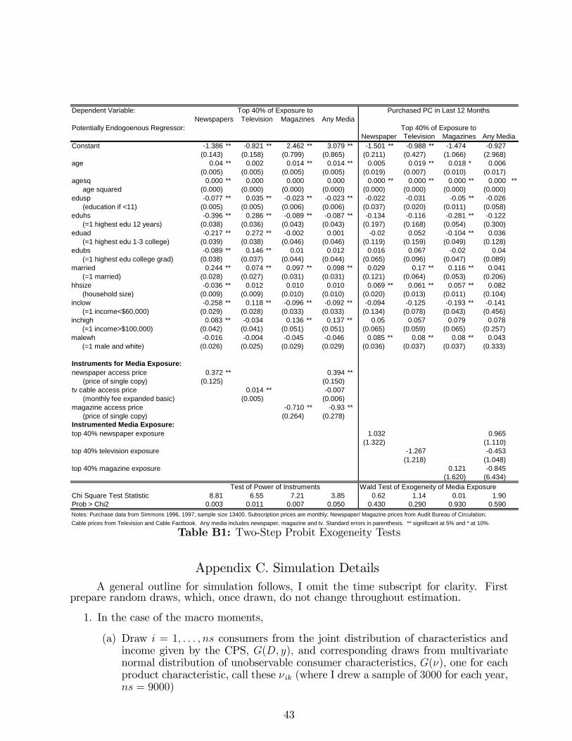
Dependent Variable: Top 40% of Exposure to Purchased PC in Last 12 MonthsNewspapers Television Magazines Any Media

Potentially Endogoenous Regressor: Top 40% of Exposure toNewspaper Television Magazines Any Media

Constant ­1.386 ** ­0.821 ** 2.462 ** 3.079 ** ­1.501 ** ­0.988 ** ­1.474 ­0.927(0.143) (0.158) (0.799) (0.865) (0.211) (0.427) (1.066) (2.968)

age 0.04 ** 0.002 0.014 ** 0.014 ** 0.005 0.019 ** 0.018 * 0.006(0.005) (0.005) (0.005) (0.005) (0.019) (0.007) (0.010) (0.017)

agesq 0.000 ** 0.000 0.000 0.000 0.000 ** 0.000 ** 0.000 ** 0.000 **age squared (0.000) (0.000) (0.000) (0.000) (0.000) (0.000) (0.000) (0.000)

edusp ­0.077 ** 0.035 ** ­0.023 ** ­0.023 ** ­0.022 ­0.031 ­0.05 ** ­0.026(education if <11) (0.005) (0.005) (0.006) (0.006) (0.037) (0.020) (0.011) (0.058)

eduhs ­0.396 ** 0.286 ** ­0.089 ** ­0.087 ** ­0.134 ­0.116 ­0.281 ** ­0.122(=1 highest edu 12 years) (0.038) (0.036) (0.043) (0.043) (0.197) (0.168) (0.054) (0.300)

eduad ­0.217 ** 0.272 ** ­0.002 0.001 ­0.02 0.052 ­0.104 ** 0.036(=1 highest edu 1­3 college) (0.039) (0.038) (0.046) (0.046) (0.119) (0.159) (0.049) (0.128)

edubs ­0.089 ** 0.146 ** 0.01 0.012 0.016 0.067 ­0.02 0.04(=1 highest edu college grad) (0.038) (0.037) (0.044) (0.044) (0.065) (0.096) (0.047) (0.089)

married 0.244 ** 0.074 ** 0.097 ** 0.098 ** 0.029 0.17 ** 0.116 ** 0.041(=1 married) (0.028) (0.027) (0.031) (0.031) (0.121) (0.064) (0.053) (0.206)

hhsize ­0.036 ** 0.012 0.010 0.010 0.069 ** 0.061 ** 0.057 ** 0.082(household size) (0.009) (0.009) (0.010) (0.010) (0.020) (0.013) (0.011) (0.104)

inclow ­0.258 ** 0.118 ** ­0.096 ** ­0.092 ** ­0.094 ­0.125 ­0.193 ** ­0.141(=1 income<$60,000) (0.029) (0.028) (0.033) (0.033) (0.134) (0.078) (0.043) (0.456)

inchigh 0.083 ** ­0.034 0.136 ** 0.137 ** 0.05 0.057 0.079 0.078(=1 income>$100,000) (0.042) (0.041) (0.051) (0.051) (0.065) (0.059) (0.065) (0.257)

malewh ­0.016 ­0.004 ­0.045 ­0.046 0.085 ** 0.08 ** 0.08 ** 0.043(=1 male and white) (0.026) (0.025) (0.029) (0.029) (0.036) (0.037) (0.037) (0.333)

Instruments for Media Exposure:newspaper access price 0.372 ** 0.394 **

(price of single copy) (0.125) (0.150)tv cable access price 0.014 ** ­0.007

(monthly fee expanded basic) (0.005) (0.006)magazine access price ­0.710 ** ­0.93 **

(price of single copy) (0.264) (0.278)Instrumented Media Exposure:top 40% newspaper exposure 1.032 0.965

(1.322) (1.110)top 40% television exposure ­1.267 ­0.453

(1.218) (1.048)top 40% magazine exposure 0.121 ­0.845

(1.620) (6.434)Test of Power of Instruments Wald Test of Exogeneity of Media Exposure

Chi Square Test Statistic 8.81 6.55 7.21 3.85 0.62 1.14 0.01 1.90Prob > Chi2 0.003 0.011 0.007 0.050 0.430 0.290 0.930 0.590Notes: Purchase data from Simmons 1996, 1997; sample size 13400. Subscription prices are monthly; Newspaper/ Magazine prices from Audit Bureau of Circulation;Cable prices from Television and Cable Factbook.  Any media includes newspaper, magazine and tv. Standard errors in parenthesis.  ** significant at 5% and * at 10%.

Table B1: Two-Step Probit Exogeneity Tests

Appendix C. Simulation DetailsA general outline for simulation follows, I omit the time subscript for clarity. First

prepare random draws, which, once drawn, do not change throughout estimation.

1. In the case of the macro moments,

(a) Draw i = 1; : : : ; ns consumers from the joint distribution of characteristics andincome given by the CPS, G(D; y); and corresponding draws from multivariatenormal distribution of unobservable consumer characteristics, G(�); one for eachproduct characteristic, call these �ik (where I drew a sample of 3000 for each year,ns = 9000)

43

(b) Draw log normal variables one for each medium combination, call these �im(wherem = 1; :::; 4):

(c) Draw uniform random variables one for each product-individual pair, call theseuij:

2. For the micro moments

(a) For each Simmons consumer i = 1; : : : ; ncons draw R times from multivariatenormal distribution of unobservable consumer characteristics, G(�); one for eachproduct characteristic, call these �ikr (where ncons = 13400):

(b) Draw R uniform random variables for each product-individual combination, callthese uijr:

(c) Draw R log normal variables one for each medium-individual combination, callthese �imr:

3. Choose an initial value of the parameters �0

4. For the macro-moments, do for i = 1; : : : ; ns

(a) Calculate �ij(�) for each product j = 1; :::; J for each period

�ij(�) =exp (� ij)

1 + exp (� ij)

� ij =Pd

gDid

0e�+#xagej +Pm

'majm+Pm

�ma2jm+f

Pm

ajm+&Pm

Pd

�mdDsidajm+

Pm

ajm�im

(b) Given �ij(�) and uij construct a J dimensional Bernoulli vector, bi(�): This de�nesthe choice set S 0, where the jth element is determined according to

bij =

�1 if �ij(�) > uij0 if �ij (�) � uij

De�ne b0i to be the Bernoulli vector generated from the initial choice of parameters,�0.

(c) Calculate

Pij(�) =expf�j + �ijg

yi� + �k:b0i;k=1 expf�k + �ikg

where �ij is value of � ln(yi�pj)+P

k xjk(�k�ik+P

dkdDid) given the ith drawand �:

(d) Calculate

sij(�) = �l2S�il�k=2S (1� �ik)Pij(�)

�0i (�0)

where �0i (�0) is the value of �l2S0�il�k=2S0 (1� �ik) using the initial value of theparameters and the initial choice set. During estimation the parameter valueswill be updated so the simulated product over the �ij will di¤er from the initial�0i (�0) in all but the �rst simulation.

44

5. Calculate the simulator for the market share

bsj = 1

ns

Xi

sij

6. For the micro-moments: For each consumer, i = 1; : : : ; ncons; calculate � ij

� ij =Pd

gDsid

0e�d + #xagej +Pm

'majm +Pm

�ma2jm +f

Pm

ajm + &Pm

Pd

�mdDsidajm

do for r = 1; : : : ; R draws

(a) Calculate �ijr(�)

�ijr(�) =exp (� ijr)

1 + exp (� ijr)

� ijr = � ij +Pm

a0jm�imr

(b) Given �ijr(�) and uijr construct a J dimensional Bernoulli vector, bir(�): Thisde�nes the choice set Sr for the rth loop, where the jth element is determinedaccording to

bijr =

�1 if �ijr(�) > uijr0 if �ijr (�) � uijr

De�ne b0ir to be the Bernoulli vector generated from the initial choice of parame-ters, �0.

(c) Calculate

Pijr(�) =expf�j + �ijrg

yi� + �k:b0ir;k=1 expf�k + �ikrg

where �ijr is value of � ln(yi � pj) +P

k xjk(�k�ikr +P

dkdDsid) given the rth

draw and �:(d) Calculate

sijr(�) = �l2Sr�il�k=2Sr (1� �ik)Pijr(�)

�0ir (�0)

where �0ir(�0) is the value of �l2Sr�il�k=2Sr (1� �ik) using the initial choice setevaluated at the initial value of the parameters, b0ir:

7. Calculate the simulator for the choice probability

csij = 1

R

Xr

sijr

The �rm choice probability (used in the micro moments) is

bBif = Xj2Jf

csij

45

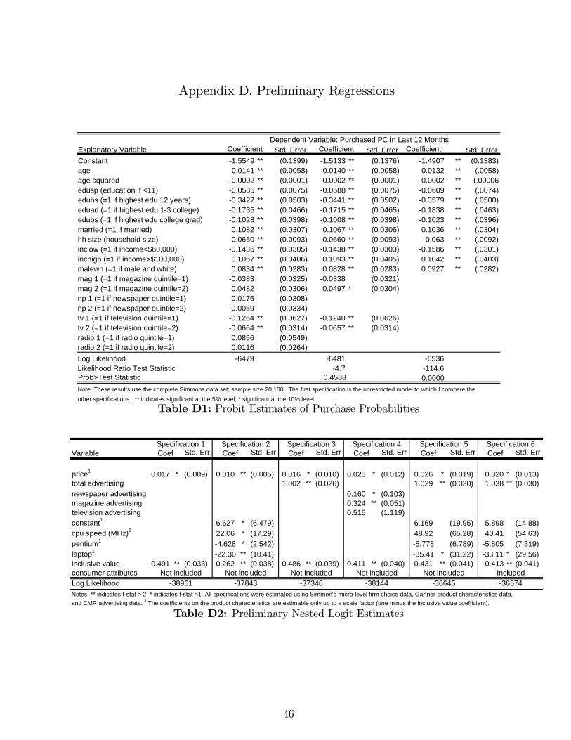
Appendix D. Preliminary Regressions

Dependent Variable: Purchased PC in Last 12 MonthsExplanatory Variable Coefficient Std. Error Coefficient Std. Error Coefficient Std. ErrorConstant ­1.5549 ** (0.1399) ­1.5133 ** (0.1376) ­1.4907 ** (0.1383)age 0.0141 ** (0.0058) 0.0140 ** (0.0058) 0.0132 ** (.0058)age squared ­0.0002 ** (0.0001) ­0.0002 ** (0.0001) ­0.0002 ** (.00006edusp (education if <11) ­0.0585 ** (0.0075) ­0.0588 ** (0.0075) ­0.0609 ** (.0074)eduhs (=1 if highest edu 12 years) ­0.3427 ** (0.0503) ­0.3441 ** (0.0502) ­0.3579 ** (.0500)eduad (=1 if highest edu 1­3 college) ­0.1735 ** (0.0466) ­0.1715 ** (0.0465) ­0.1838 ** (.0463)edubs (=1 if highest edu college grad) ­0.1028 ** (0.0398) ­0.1008 ** (0.0398) ­0.1023 ** (.0396)married (=1 if married) 0.1082 ** (0.0307) 0.1067 ** (0.0306) 0.1036 ** (.0304)hh size (household size) 0.0660 ** (0.0093) 0.0660 ** (0.0093) 0.063 ** (.0092)inclow (=1 if income<$60,000) ­0.1436 ** (0.0305) ­0.1438 ** (0.0303) ­0.1586 ** (.0301)inchigh (=1 if income>$100,000) 0.1067 ** (0.0406) 0.1093 ** (0.0405) 0.1042 ** (.0403)malewh (=1 if male and white) 0.0834 ** (0.0283) 0.0828 ** (0.0283) 0.0927 ** (.0282)mag 1 (=1 if magazine quintile=1) ­0.0383 (0.0325) ­0.0338 (0.0321)mag 2 (=1 if magazine quintile=2) 0.0482 (0.0306) 0.0497 * (0.0304)np 1 (=1 if newspaper quintile=1) 0.0176 (0.0308)np 2 (=1 if newspaper quintile=2) ­0.0059 (0.0334)tv 1 (=1 if television quintile=1) ­0.1264 ** (0.0627) ­0.1240 ** (0.0626)tv 2 (=1 if television quintile=2) ­0.0664 ** (0.0314) ­0.0657 ** (0.0314)radio 1 (=1 if radio quintile=1) 0.0856 (0.0549)radio 2 (=1 if radio quintile=2) 0.0116 (0.0264)Log Likelihood ­6479 ­6481 ­6536Likelihood Ratio Test Statistic ­4.7 ­114.6Prob>Test Statistic 0.4538 0.0000Note: These results use the complete Simmons data set; sample size 20,100.  The first specification is the unrestricted model to which I compare theother specifications.  ** indicates significant at the 5% level; * significant at the 10% level.

Table D1: Probit Estimates of Purchase Probabilities

Specification 1 Specification 2 Specification 3 Specification 4 Specification 5 Specification 6Variable Coef Std. Err Coef Std. Err Coef Std. Err Coef Std. Err Coef Std. Err Coef Std. Err

price1 0.017 * (0.009) 0.010 ** (0.005) 0.016 * (0.010) 0.023 * (0.012) 0.026 * (0.019) 0.020 * (0.013)total advertising 1.002 ** (0.026) 1.029 ** (0.030) 1.038 ** (0.030)newspaper advertising 0.160 * (0.103)magazine advertising 0.324 ** (0.051)television advertising 0.515 (1.119)constant1 6.627 * (6.479) 6.169 (19.95) 5.898 (14.88)cpu speed (MHz)1 22.06 * (17.29) 48.92 (65.28) 40.41 (54.63)pentium1 ­4.628 * (2.542) ­5.778 (6.789) ­5.805 (7.319)laptop1 ­22.30 ** (10.41) ­35.41 * (31.22) ­33.11 * (29.56)inclusive value 0.491 ** (0.033) 0.262 ** (0.038) 0.486 ** (0.039) 0.411 ** (0.040) 0.431 ** (0.041) 0.413 ** (0.041)consumer attributes Not included Not included Not included Not included Not included IncludedLog Likelihood ­38961 ­37843 ­37348 ­38144 ­36645 ­36574Notes: ** indicates t­stat > 2; * indicates t­stat >1. All specifications were estimated using Simmon's micro­level firm choice data, Gartner product characteristics data,and CMR advertising data. 1 The coefficients on the product characteristics are estimable only up to a scale factor (one minus the inclusive value coefficient).

Table D2: Preliminary Nested Logit Estimates

46

OLS OLS IV IV IV IVVariable (i) (ii) (iii) (iv) (v) (vi)

price ­0.05 * ­0.04 * ­0.71 ** ­1.07 ** ­2.41 ** ­2.46 **(0.04) (0.04) (0.13) (0.17) (0.51) (0.41)

cpu speed 0.16 ** 0.17 ** 0.07 0.06 0.17 * 0.07 *(0.08) (0.08) (0.08) (0.08) (0.14) (0.11)

pentium ­0.36 ** 0.04 ­0.68 ** ­0.85 ** 1.51 ** 2.04 **(0.09) (0.14) (0.11) (0.19) (0.29) (0.38)

laptop ­1.27 ** ­1.25 ** 1.99 ** 2.35 ** 3.82 ** 3.83 **(0.09) (0.09) (0.16) (0.20) (0.58) (0.47)

acer 1.64 ** 1.65 ** 1.67 **(0.16) (0.17) (0.20)

apple 1.81 ** 0.62 ** 0.98 *(0.20) (0.29) (0.56)

compaq 1.77 ** 1.72 ** 1.66 **(0.16) (0.17) (0.21)

dell 0.72 ** 0.43 ** 0.06(0.16) (0.17) (0.25)

gateway 1.98 ** 1.43 ** 0.69 **(0.17) (0.21) (0.33)

hp ­0.13 ­0.26 * ­0.43 **(0.17) (0.18) (0.22)

ibm 1.01 ** 0.64 ** 0.13(0.16) (0.19) (0.28)

micron 0.55 ** ­0.71 ** ­2.40 **(0.17) (0.28) (0.56)

pbell 2.24 ** 2.18 ** 2.10 **(0.17) (0.19) (0.23)

Constant ­12.64 ** ­13.83 ** ­12.83 ** ­13.99 ** ­13.33 ** ­14.20 **(0.89) (0.89) (0.90) (0.90) (1.32) (1.21)

First StageAdjusted R2 0.13 0.30 0.42 0.53 0.33 0.49F­statistic 126.47 112.7 210.69 143.76Prob > F 0.00 0.00 0.00 0.00InstrumentsBLP 95 Series approximation X XBLP 99 Direct approximation X XNotes: The dependent variable is ln (s_j)­ln (s_0) based on 2112 observations.   All regressions include time dummies.Asymptotically robust standard errors are in parenthesis. ** indicates t­stat>2; * indicates t­stat>1.  BLP series approximationIV are the sum of the values of the same characteristics of other products offered by the same firm, the sum of the values ofthe same characteristics of all products offered by rival firms, the number of own­firm products, and the number of rival firmproducts.  The more direct approximation IV are based on BLP 1999.  These are used in the full model and described in the paper.

Table D3: Logit IV Results

47

References

Ackerberg, D. (2001): Empirically Distinguishing Informative and Prestige E¤ects of Adver-tising, RAND Journal of Economics, 32, 100-118.

Ackerberg, D. (2003): Advertising, Learning, and Consumer Choice in Experience GoodsMarkets: A Structural Empirical Examination, International Economic Review, 44,1007-1040.

Anand, B., and R. Shachar (2004): �Advertising, the Matchmaker,�Harvard Business SchoolWorking Paper No. 02-057.

Anderson, S., and A. de Palma, and J.F. Thisse (1989): Demand for Di¤erentiated Prod-ucts, Discrete Choice Models, and the Characteristics Approach, Review of EconomicStudies 56, 21-35.

Andrews, D. (1988): Chi-square Diagnostic Tests for Econometric Models, Journal of Econo-metrics, 37, 135-156.

Bajari, P., and C. L. Benkard (2005): Demand Estimation with Heterogenous Consumersand Unobserved Product Characteristics: A Hedonic Approach, Journal of PoliticalEconomy, 113, 1239-1276.

Berry, S. (1994): Estimating Discrete Choice Models of Product Di¤erentiation, Rand Jour-nal of Economics, 25, 242-262.

Berry, S., J. Levinsohn, and A. Pakes (1995): Automobile Prices in Market Equilibrium,Econometrica, 63, 841-890.

Berry, S., J. Levinsohn, and A. Pakes (1999): Voluntary Export Restraints on Automobiles:Evaluating a Trade Policy, American Economic Review, 89, 400-430.

Berry, S., J. Levinsohn, and A. Pakes (2004): Di¤erentiated Products Demand Systems froma Combination of Micro and Macro Data: The New Car Market, Journal of PoliticalEconomy, 112, 68-105.

Bresnahan, T. (1989): Empirical Studies of Industries with Market Power, in Handbook ofIndustrial Organization, ed. by R. Schmalensee and R. Willig. North-Holland, NewYork and Oxford: Elsevier Science Publishers, Chapter 17.

Chamberlain, G. (1987): Asymptotic E¢ ciency in Estimation with Conditional MomentRestrictions, Journal of Econometrics, 34, 305-344.

Chiang, J., S. Chib, and C. Narasimhan (1999): Markov Chain Monte Carlo and Models ofConsideration Set and Parameter Heterogeneity, Journal of Econometrics, 89, 223-248.

Ching, A., T. Erdem, and M. Keane (2007): The Price Consideration Model of BrandChoice,�forthcoming, Journal of Applied Econometrics

Erdem, T., and M. Keane (1996): Decision-making Under Uncertainty: Capturing DynamicBrand Choice Processes in Turbulent Consumer Goods Markets, Marketing Science,15, 1-20.

Geweke, J. (1988): Antithetic Acceleration of Monte Carlo Integration in Bayesian Inference,Journal of Econometrics, 38, 73-89.

Goeree, M.S. (2002): �Informative Advertising and the US Personal Computer Market: AStructural Empirical Examination,�Ph.D. Dissertation, University of Virginia.

Goeree, M.S. (2003): �Was Mr. Hewlett Right? Mergers, Advertising, and the PC Industry,�Unpublished Manuscript, Claremont McKenna College.

Goeree, M.S. (2008): �Limited Information and Advertising in the US Personal Computer In-dustry, Supplementary Material: Miscellaneous,�Econometrica Supplementary Ma-terial, http://www.econometricsociety.org/ecta/supmat/

Gourieroux, C., A. Monfort, E. Renault, and A. Trognon (1987): Generalized Residuals,Journal of Econometrics, 34, 5-32.

Grossman, G., and C. Shapiro (1984): Informative Advertising with Di¤erentiated Products,Review of Economic Studies, 51, 63-82.

Hendel, I. (1999): Estimating Multiple-Discrete Choice Models: An Application to Comput-erization Returns, Review of Economic Studies, 66, 423-46.

Leslie, P. (2004): Price Discrimination in Broadway Theater, Rand Journal of Economics,35, 520-541.

Mehta, N., S.Rajiv, and K. Srinivasan (2003): Price Uncertainty and Consumer Search: AStructural Model of Consideration Set Formation, Marketing Science, 22, 58-84.

Milgrom, P., and J. Roberts (1986): Price and Advertising Signals of Product Quality,Journal of Political Economy, 94, 796-821.

Nevo, A. (2000): A Practitioner�s Guide to Estimation of Random Coe¢ cients Logit Modelsof Demand, Journal of Economics and Management Strategy, 9, 513-548.

Nierop, E., R. Paap, B.Bronnenberg, P. Franses, and M. Wedel (2005): �Retrieving Unob-served Consideration Sets from Household Panel Data,�UCLA Anderson WorkingPaper.

Pakes, A., and D. Pollard (1989): Simulation and the Asymptotics of Optimization Estima-tors, Econometrica, 57, 1027-1057.

Petrin, A. (2002): Quantifying the Bene�ts of New Products: The Case of the Minivan,Journal of Political Economy, 110, 705-729.

Rivers, D., and Q. Vuong (1988): Limited Information Estimators and Exogeneity Tests forSimultaneous Probit Models, Journal of Econometrics, 39, 347-366.

Shum, M. (2004): Does Advertising Overcome Brand Loyalty? Evidence from the BreakfastCereals Market, Journal of Economics and Management Strategy, 13, 241-272.

Smith, R.J., and R. Blundell (1986): An Exogeneity Test for a Simultaneous Equation TobitModel with an Application to Labor Supply, Econometrica, 54, 679-85.

Stern, S. (1997): Simulation-Based Estimation, Journal of Economic Literature, 35, 2006-2039.

Stern, S. (2000): Simulation Based Inference in Econometrics: Motivation and Methods,in Simulation-Based Inference in Econometrics: Methods and Applications, ed. byMariano, Weeks, and Schuermann. Cambridge, U.K.: Cambridge University Press.

Vuong, Q.H. (1989): Likelihood Ratio Tests for Model Selection and Non-Nested Hypotheses,Econometrica, 57, 307-333.

Wooldridge, J. (2002): Econometric Analysis of Cross Section and Panel Data, CambridgeM.A.: MIT Press.