linear control of manipulators

CHAPTER 9

Linear control of manipulators

9.1 INTRODUCTION

9.2 FEEDBACK AND CLOSED-LOOP CONTROL

9.3 SECOND-ORDER LINEAR SYSTEMS

9.4 CONTROL OF SECOND-ORDER SYSTEMS

9.5 CONTROL-LAW PARTITIONING

9.6 TRAJECTORY-FOLLOWING CONTROL

9.7 DISTURBANCE REJECTION

9.8 CONTINUOUS VS. DISCRETE TIME CONTROL

9.9 MODELING AND CONTROL OF A SINGLE JOINT9.10 ARCHITECTURE OF AN INDUSTRIAL-ROBOT CONTROLLER

9.1 INTRODUCTION

Armed with the previous material, we now have the means to calculate joint-position time histories that correspond to desired end-effector motions throughspace. In this chapter, we begin to discuss how to cause the manipulator actually toperform these desired motions.

The control methods that we wifi discuss fall into the class called linear-controlsystems. Strictly speaking, the use of linear-control techniques is valid only whenthe system being studied can be modeled mathematically by linear differentialequations. For the case of manipulator control, such linear methods must essentiallybe viewed as approximate methods, for, as we have seen in Chapter 6, the dynamicsof a manipulator are more properly represented by a nonlinear differential equation.Nonetheless, we wifi see that it is often reasonable to make such approximations,and it also is the case that these linear methods are the ones most often used incurrent industrial practice.

Finally, consideration of the linear approach will serve as a basis for themore complex treatment of nonlinear control systems in Chapter 10. Although weapproach linear control as an approximate method for manipulator control, thejustification for using linear controllers is not only empirical. In Chapter 10, wewill prove that a certain linear controller leads to a reasonable control systemeven without resorting to a linear approximation of manipulator dynamics. Readersfamiliar with linear-control systems might wish to skip the first four sections of thecurrent chapter.

262

Section 9.2 Feedback and closed-loop control 263

9.2 FEEDBACK AND CLOSED-LOOP CONTROL

We will model a manipulator as a mechanism that is instrumented with sensorsat each joint to measure the joint angle and that has an actuator at each joint toapply a torque on the neighboring (next higher) link.1. Although other physicalarrangements of sensors are sometimes used, the vast majority of robots have aposition sensor at each joint. Sometimes velocity sensors (tachometers) are alsopresent at the joints. Various actuation and transmission schemes are prevalent inindustrial robots, but many of these can be modeled by supposing that there is asingle actuator at each joint.

We wish to cause the manipulator joints to follow prescribed position trajec-tories, but the actuators are commanded in terms of torque, so we must use somekind of control system to compute appropriate actuator commands that will realizethis desired motion. Almost always, these torques are determined by using feedbackfrom the joint sensors to compute the torque required.

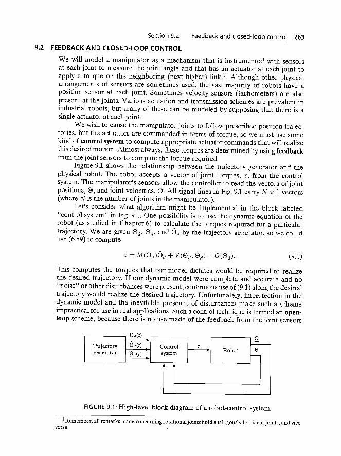
Figure 9.1 shows the relationship between the trajectory generator and thephysical robot. The robot accepts a vector of joint torques, r, from the controlsystem. The manipulator's sensors allow the controller to read the vectors of jointpositions, e, and joint velocities, e. All signal lines in Fig. 9.1 carry N x 1 vectors(where N is the number of joints in the manipulator).

Let's consider what algorithm might be implemented in the block labeled"control system" in Fig. 9.1. One possibility is to use the dynamic equation of therobot (as studied in Chapter 6) to calculate the torques required for a particulartrajectory. We are given ed, ®d, and °d by the trajectory generator, so we coulduse (6.59) to compute

r = + V(Od, ed) + G(ed). (9.1)

This computes the torques that our model dictates would be required to realizethe desired trajectory. If our dynamic model were complete and accurate and no"noise" or other disturbances were present, continuous use of (9.1) along the desiredtrajectory would realize the desired trajectory. Unfortunately, imperfection in thedynamic model and the inevitable presence of disturbances make such a schemeimpractical for use in real applications. Such a control technique is termed an open-loop scheme, because there is no use made of the feedback from the joint sensors

FIGURE 9.1: High-level block diagram of a robot-control system.

1Remember all remarks made concerning rotational joints holdanalogously for linear joints, and viceversa

264 Chapter 9 Linear control of manipulators

(i.e., (9.1) is a function oniy of the desired trajectory, ®d' and its derivatives, and nota function of 0, the actual trajectory).

Generally, the only way to build a high-performance control system is to makeuse of feedback from joint sensors, as indicated in Fig. 9.1. Typically, this feedbackis used to compute any servo error by finding the difference between the desiredand the actual position and that between the desired and the actual velocity:

E = —0,

(9.2)

The control system can then compute how much torque to require of the actuatorsas some function of the servo error. Obviously, the basic idea is to compute actuatortorques that would tend to reduce servo errors. A control system that makes use offeedback is called a closed-loop system. The "loop" closed by such a control systemaround the manipulator is apparent in Fig. 9.1.

The central problem in designing a control system is to ensure that the resultingclosed-loop system meets certain performance specifications. The most basic suchcriterion is that the system remain stable. For our purposes, we wifi define a systemto be stable if the errors remain "small" when executing various desired trajectorieseven in the presence of some "moderate" disturbances. It should be noted that animproperly designed control system can sometimes result in unstable performance,in which servo errors are enlarged instead of reduced. Hence, the first task of acontrol engineer is to prove that his or her design yields a stable system; the secondis to prove that the closed-loop performance of the system is satisfactory. In practice,such "proofs" range from mathematical proofs based on certain assumptions andmodels to more empirical results, such as those obtained through simulation orexperimentation.

Figure 9.1, in which all signals lines represent N xl vectors, summarizes the factthat the manipulator-control problem is a multi-input, multi-output (MIMO) controlproblem. In this chapter, we take a simple approach to constructing a control systemby treating each joint as a separate system to be controlled. Hence, for an N-jointedmanipulator, we will design N independent single-input, single-output (SISO)control systems. This is the design approach presently adopted by most industrial-robot suppliers. This independent joint control approach is an approximate methodin that the equations of motion (developed in Chapter 6) are not independent, butrather are highly coupled. Later, this chapter wifi present justification for the linearapproach, at least for the case of highly geared manipulators.

9.3 SECOND-ORDER LINEAR SYSTEMS

Before considering the manipulator control problem, let's step back and start byconsidering a simple mechanical system. Figure 9.2 shows a block of mass in attachedto a spring of stiffness k and subject to friction of coefficient b. Figure 9.2 also indicatesthe zero position and positive sense of x, the block's position. Assuming a frictionalforce proportional to the block's velocity, a free-body diagram of the forces actingon the block leads directly to the equation of motion,

niI+bi+kx =0. (9.3)

Section 9.3 Second-order linear systems 265

FIGURE 9.2: Spring—mass system with friction.

Hence, the open-loop dynamics of this one-degree-of-freedom system are describedby a second-order linear constant-coefficient differential equation [1]. The solutionto the differential equation (9.3) is a time function, x (t), that specifies the motionof the block. This solution will depend on the block's initial conditions—that is, itsinitial position and velocity.

We wifi use this simple mechanical system as an example with which to reviewsome basic control system concepts. Unfortunately, it is impossible to do justice tothe field of control theory with only a brief introduction here. We wifi discuss thecontrol problem, assuming no more than that the student is familiar with simpledifferential equations. Hence, we wifi not use many of the popular tools of thecontrol-engineering trade. For example, Laplace transforms and other commontechniques neither are a prerequisite nor are introduced here. A good reference forthe field is [4].

Intuition suggests that the system of Fig. 9.2 might exhibit several differentcharacteristic motions. For example, in the case of a very weak spring (i.e., k small)and very heavy friction (i.e., b large) one imagines that, if the block were perturbed,it would return to its resting position in a very slow, sluggish manner. However,with a very stiff spring and very low friction, the block might oscifiate several timesbefore coming to rest. These different possibilities arise because the character of thesolution to (9.3) depends upon the values of the parameters in, b, and k.

From the study of differential equations [1], we know that the form of thesolution to an equation of the form of (9.3) depends on the roots of its characteristicequation,

ins2+bs-j-k=O. (9.4)

This equation has the roots

bS1

— 2in+

2iii

b — 4mk(9.5)

2m 2in

The location of and s2 (sometimes called the poles of the system) in thereal—imaginary plane dictate the nature of the motions of the system. If and s2are real, then the behavior of the system is sluggish and nonoscillatory. If andare complex (i.e., have an imaginary component) then the behavior of the system is


oscifiatory. If we include the special limiting case between these two behaviors, wehave three classes of response to study:

1. Real and Unequal Roots. This is the case when b2 > 4 ink; that is, frictiondominates, and sluggish behavior results. This response is called overdamped.

2. Complex Roots. This is the case when b2 <4 ink; that is, stiffness dominates,and oscifiatory behavior results. This response is called underdamped.

3. Real and Equal Roots. This is the special case when b2 = 4 ink; that is,friction and stiffness are "balanced," yielding the fastest possible nonosdillatoryresponse. This response is called critically damped.

The third case (critical damping) is generally a desirable situation: the systemnulls out nonzero initial conditions and returns to its nominal position as rapidly aspossible, yet without oscillatory behavior.

Real and unequal roots

It can easily be shown (by direct substitution into (9.3)) that the solution, x(t), givingthe motion of the block in the case of real, unequal roots has the form

x(t) = + c2eS2t, (9.6)

where s1 and s2 are given by (9.5). The coefficients c1 and c2 are constants that canbe computed for any given set of initial conditions (i.e., initial position and velocityof the block).

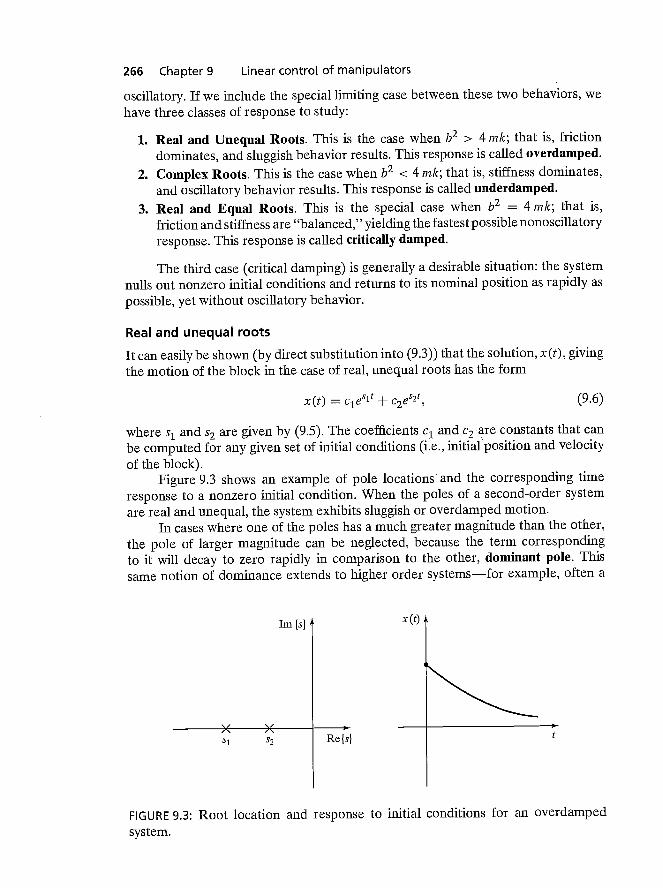
Figure 9.3 shows an example of pole locations• and the corresponding timeresponse to a nonzero initial condition. When the poles of a second-order systemare real and unequal, the system exhibits sluggish or overdamped motion.

In cases where one of the poles has a much greater magnitude than the other,the pole of larger magnitude can be neglected, because the term correspondingto it wifi decay to zero rapidly in comparison to the other, dominant pole. Thissame notion of dominance extends to higher order systems—for example, often a

Tm )s}x(t)

,\ /\Rejs} t

FIGURE 9.3: Root location and response to initial conditions for an overdampedsystem.


third-order system can be studied as a second-order system by considering only twodominant poles.

EXAMPLE 9.1

Determine the motion of the system in Fig. 9.2 if parameter values are in = 1, b = 5,and k = 6 and the block (initially at rest) is released from the position x = —1.

The characteristic equation is

(9.7)

which has the roots s1 = —2 and = Hence, the response has the form

x(t) = + c2e_3t (9.8)

We now use the given initial conditions, x(0) = —1 and i(0) = 0, to compute c1 andc2. To satisfy these conditions at t = 0, we must have

Ci + C2 = —1

and—2c1 — 3c2 = 0, (9.9)

which are satisfied by c1 = —3 and c2 = 2. So, the motion of the system for t ? 0 isgiven by

x(t) = _3e_2t + 2e_3t. (9.10)

Complex roots

For the case where the characteristic equation has complex roots of the form

= A + /Li,

= A — (9.11)

it is stifi the case that the solution has the form

x(t) = c1eS1t + c2eS2t. (9.12)

However, equation (9.12) is difficult to use directly, because it involves imaginarynumbers explicitly. It can be shown (see Exercise 9.1) that Euler's formula,

= cosx + i sinx, (9.13)

allows the solution (9.12) to be manipulated into the form

x(t) = cieAt cos(/Lt) + (9.14)

As before, the coefficients c1 and c2 are constants that can be computed for anygiven set of initial conditions (i.e., initial position and velocity of the block). If wewrite the constants c1 and c2 in the form

C1 = r cos 8,

c2=rsin8, (9.15)


then (9.14) can be written in the form

x(t) = rext — 8), (9.16)

where

r

8 = Atan2(c2, c1). (9.17)

In this form, it is easier to see that the resulting motion is an oscifiation whoseamplitude is exponentially decreasing toward zero.

Another common way of describing oscillatory second-order systems is interms of damping ratio and natural frequency. These terms are defined by theparameterization of the characteristic equation given by

+ + = 0, (9.18)

where is the damping ratio (a dimensionkss number between 0 and 1) andw71 is the natural frequency.2 Relationships between the pole locations and theseparameters are

=

and

= (9.19)

In this terminology, the imaginary part of the poles, is sometimes called thedamped natural frequency. For a damped spring—mass system such as the one inFig. 9.2, the damping ratio and natural frequency are, respectively,

b

= (9.20)

When no damping is present (b = 0 in our example), the damping ratio becomeszero; for critical damping (b2 = 4km), the damping ratio is 1.

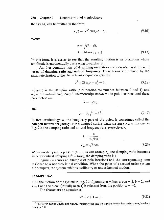
Figure 9.4 shows an example of pole locations and the corresponding timeresponse to a nonzero initial condition. When the poles of a second-order systemare complex, the system exhibits oscifiatory or underdamped motion.

EXAMPLE 9.2

Find the motion of the system in Fig. 9.2 if parameter values are m = 1, b = 1, andk = 1 and the block (initially at rest) is released from the position x = —1.


s2+s+1=0, (9.21)

2The terms damping ratio and natural frequency can also be applied to overdamped systems, in whichcase > 1.0.


Tm{s} x(t)

X

Re(s} \.JX

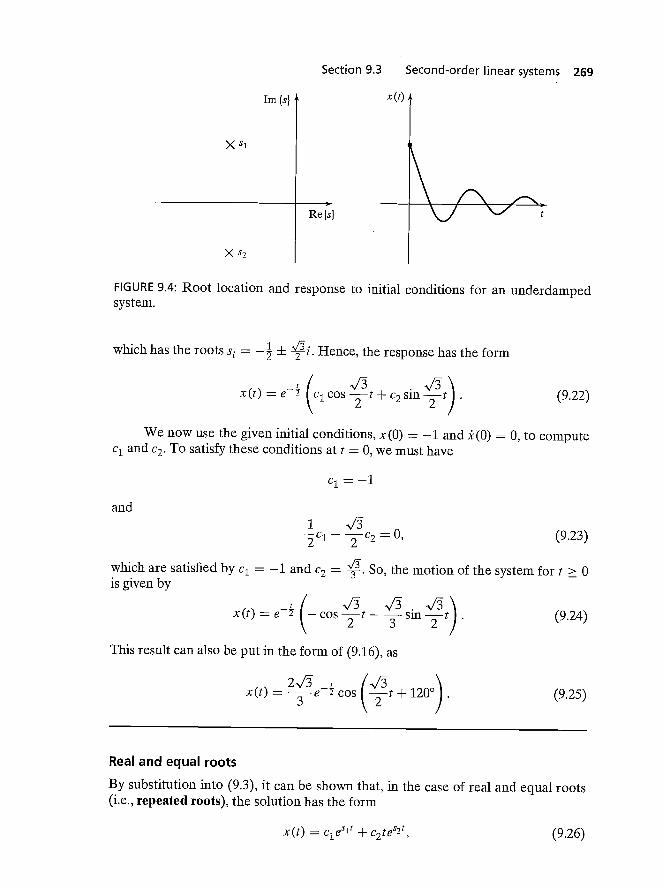
FIGURE 9.4: Root location and response to initial conditions for an underdampedsystem.

which has the roots = + Hence, the response has the form

x(t) = e 2 c1 cos + c2 sin . (9.22)

We now use the given initial conditions, x (0) = —1 and (0) = 0, to computec1 and c2. To satisfy these conditions at t = 0, we must have

C1 = —1

and1

— = 0, (9.23)

which are satisfied by c1 = —1 and c2 = So, the motion of the system for t 0is given by

x(t) = e 2 cos — sin (9.24)

This result can also be put in the form of (9.16), as

= cos (4t + 1200). (9.25)

Real and equal roots

By substitution into (9.3), it can be shown that, in the case of real and equal roots(i.e., repeated roots), the solution has the form

x(t) = c1eSlt + c2teS2t, (9.26)


Tm(s) x(t)

Re(s)

FIGURE 9.5: Root location and response to initial conditions for a critically dampedsystem.

where, in this case, s1 = s2 = (9.26) can be written

x(t) = (c1 + (9.27)

In case it is not clear, a quick application of l'Hôpital's rule [2] shows that, forany c1, c2, and a,

urn (c1 + c7t)e_at = 0. (9.28)t-+oo

Figure 9.5 shows an example of pole locations and the corresponding timeresponse to a nonzero initial condition. When the poles of a second-order systemare real and equal, the system exhibits critically damped motion, the fastest possible

nonoscifiatory response.

EXAMPLE 9.3

Work out the motion of the system in Fig. 9.2 if parameter values are in = 1, b = 4,and k = 4 and the block (initially at rest) is released from the position x = —1.


(9.29)

which has the roots s1 = s2 = —2. Hence, the response has the form

x(t) = (c1 + c7t)e_2t. (9.30)

We now use the given initial conditions, x(0) = —1 and ±(0) = 0, to calculatec1 and c2. To satisfy these conditions at t = 0, we must have

Cl = —1

and—2c1 + c2 = 0, (9.31)

which are satisfied by c1 = —1 and c2 = —2. So, the motion of the system for t 0

is given byx(t) = (—1 — 2t)e_2t. (9.32)

Section 9.4 Control of second-order systems 271

In Examples 9.1 through 9.3, all the systems were stable. For any passivephysical system like that of Fig. 9.2, this will be the case. Such mechanical systemsalways have the properties

in >0,

b > 0, (9.33)

k >0.

In the next section, we wifi see that the action of a control system is, in effect, tochange the value of one or more of these coefficients. It will then be necessary toconsider whether the resulting system is stable.

9.4 CONTROL OF SECOND-ORDER SYSTEMS

Suppose that the natural response of our second-order mechanical system is notwhat we wish it to be. Perhaps it is underdamped and oscillatory, and we would likeit to be critically damped; or perhaps the spring is missing altogether (k = 0), so thesystem never returns to x = 0 if disturbed. Through the use of sensors, an actuator,and a control system, we can modify the system's behavior as desired.

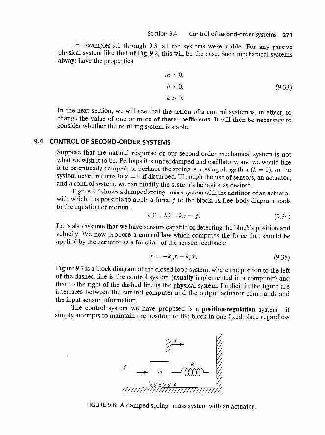
Figure 9.6 shows a damped spring—mass system with the addition of an actuatorwith which it is possible to apply a force f to the block. A free-body diagram leadsto the equation of motion,

nil + + kx = f. (9.34)

Let's also assume that we have sensors capable of detecting the block's position andvelocity. We now propose a control law which computes the force that should beapplied by the actuator as a function of the sensed feedback:

f = — (9.35)

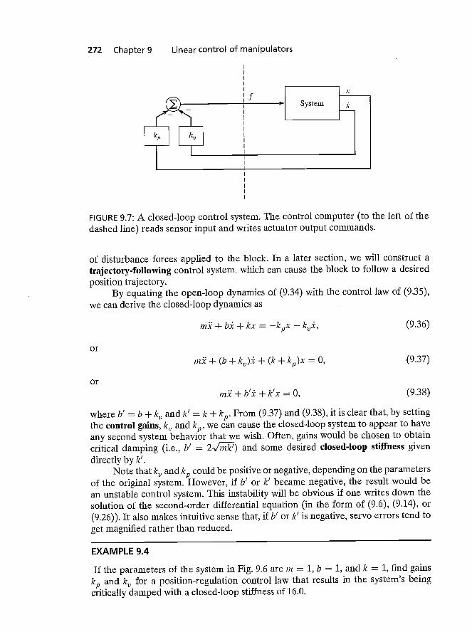
Figure 9.7 is a block diagram of the closed-loop system, where the portion to the leftof the dashed line is the control system (usually implemented in a computer) andthat to the right of the dashed line is the physical system. Implicit in the figure areinterfaces between the control computer and the output actuator commands andthe input sensor information.

The control system we have proposed is a position-regulation system—itsimply attempts to maintain the position of the block in one fixed place regardless

/

FIGURE 9.6: A damped spring—mass system with an actuator.


FIGURE 9.7: A closed-loop control system. The control computer (to the left of thedashed line) reads sensor input and writes actuator output commands.

of disturbance forces applied to the block. In a later section, we will construct atrajectory-following control system, which can cause the block to follow a desiredposition trajectory.

By equating the open-loop dynamics of (9.34) with the control law of (9.35),we can derive the closed-loop dynamics as

ml + bi + kx = — (9.36)

or=0, (9.37)

orml +

b' k' = k and (9.38), it is clear that, by settingthe control gains, and we can cause the closed-loop system to appear to haveany second system behavior that we wish. Often, gains would be chosen to obtaincritical damping (i.e., b' = and some desired closed-loop stiffness givendirectly by k'.

Note that and could be positive or negative, depending on the parametersof the original system. However, if b' or k' became negative, the result would bean unstable control system. This instability will be obvious if one writes down thesolution of the second-order differential equation (in the form of (9.6), (9.14), or(9.26)). It also makes intuitive sense that, if b' or k' is negative, servo errors tend toget magnified rather than reduced.

EXAMPLE 9.4

If the parameters of the system in Fig. 9.6 are in = 1, b = 1, and k = 1, find gainsand for a position-regulation control law that results in the system's being

critically damped with a closed-loop stiffness of 16.0.

x

Section 9.5 Control-law partitioning 273

If we wish k' to be 16.0, then, for critical damping, we require that b' == 8.0. Now, k = 1 and b = 1, so we need

= 15.0,

= 7.0. (9.39)

9.5 CONTROL-LAW PARTITIONING

In preparation for designing control laws for more complicated systems, let usconsider a slightly different controller structure for the sample problem of Fig. 9.6.In this method, we wifi partition the controller into a model-based portion and aservo portion. The result is that the system's parameters (i.e., in, b, and k, in this case)appear only in the model-based portion and that the servo portion is independentof these parameters. At the moment, this distinction might not seem important,but it wifi become more obviously important as we consider nonlinear systemsin Chapter 10. We will adopt this control-law partitioning approach throughoutthe book.

The open-loop equation of motion for the system is

ml + hi + kx = f. (9.40)

We wish to decompose the controller for this system into two parts. In this case, themodel-based portion of the control law wifi make use of supposed knowledge of in,b, and k. This portion of the control law is set up such that it reduces the system sothat it appears to be a unit mass. This will become clear when we do Example 9.5.The second part of the control law makes use of feedback to modify the behavior ofthe system. The model-based portion of the control law has the effect of making thesystem appear as a unit mass, so the design of the servo portion is very simple—gainsare chosen to control a system composed of a single unit mass (i.e., no friction, nostiffness).

The model-based portion of the control appears in a control law of the form

(9.41)

where u and are functions or constants and are chosen so that, if f'is taken as thenew input to the system, the system appears to be a unit mass. With this structure ofthe control law, the system equation (the result of combining (9.40) and (9.41)) is

inl+bi+kx =af'+tl. (9.42)

Clearly, in order to make the system appear as a unit mass from the f' input, forthis particular system we should choose a and as follows:

a = in,

(9.43)

Making these assignments and plugging them into (9.42), we have the systemequation

I = f'. (9.44)


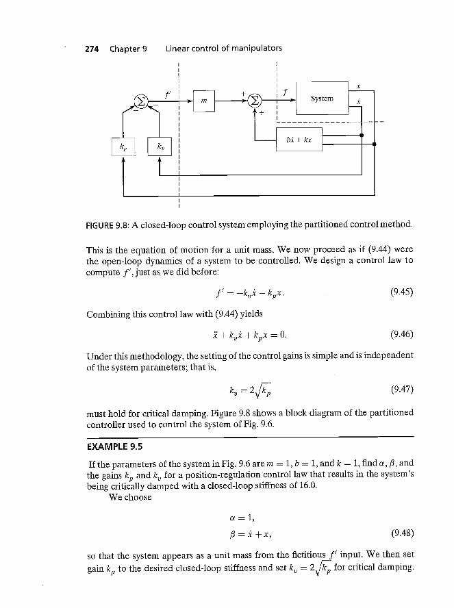
FIGURE 9.8: A closed-loop control system employing the partitioned control method.

This is the equation of motion for a unit mass. We now proceed as if (9.44) werethe open-loop dynamics of a system to be controlled. We design a control law tocompute f ', just as we did before:

f' = —

Combining this control law with (9.44) yields

=0.

(9.45)

(9.46)

Under this methodology, the setting of the control gains is simple and is independentof the system parameters; that is,

= (9.47)

must hold for critical damping. Figure 9.8 shows a block diagram of the partitionedcontroller used to control the system of Fig. 9.6.

EXAMPLE 9.5

If the parameters of the system in Fig. 9.6 are in = 1, b = 1, and k = 1, find a, andthe gains and for a position-regulation control law that results in the system'sbeing critically damped with a closed-loop stiffness of 16.0.

We choose

a = 1,

(9.48)

so that the system appears as a unit mass from the fictitious f'input. We then setgain to the desired closed-loop stiffness and set = for critical damping.

Section 9.6 Trajectory-following control 275

This gives

= 16.0,

= 8.0. (9.49)

9.6 TRAJECTORY-FOLLOWING CONTROL

Rather than just maintaining the block at a desired location, let us enhance ourcontroller so that the block can be made to follow a trajectory. The trajectory isgiven by a ftnction of time, xd(t), that specifies the desired position of the block.We assume that the trajectory is smooth (i.e., the first two derivatives exist) and thatour trajectory generator provides xd, ia, and 1d at all times t. We define the servoerror between the desired and actual trajectory as e = xd — x. A servo-control lawthat will cause trajectory following is

(9.50)

We see that (9.50) is a good choice if we combine it with the equation of motion ofa unit mass (9.44), which leads to

I (9.51)

or

(9.52)

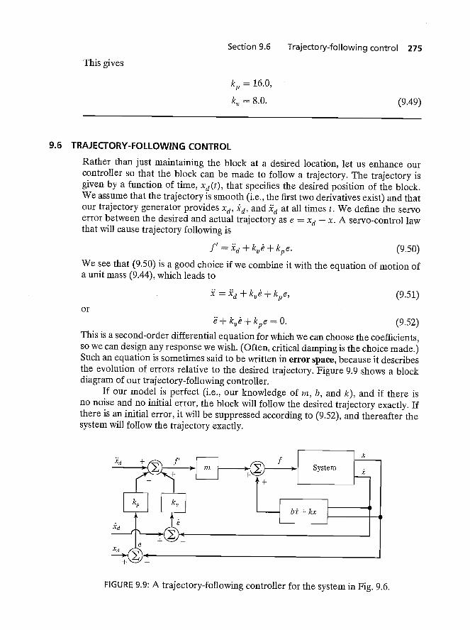
This is a second-order differential equation for which we can choose the coefficients,so we can design any response we wish. (Often, critical damping is the choice made.)Such an equation is sometimes said to be written in error space, because it describesthe evolution of errors relative to the desired trajectory. Figure 9.9 shows a blockdiagram of our trajectory-following controller.

If our model is perfect (i.e., our knowledge of in, b, and k), and if there isno noise and no initial error, the block will follow the desired trajectory exactly. Ifthere is an initial error, it will be suppressed according to (9.52), and thereafter thesystem wifi follow the trajectory exactly.

FIG URE 9.9: A trajectory-following controller for the system in Fig. 9.6.


9.7 DISTURBANCE REJECTION

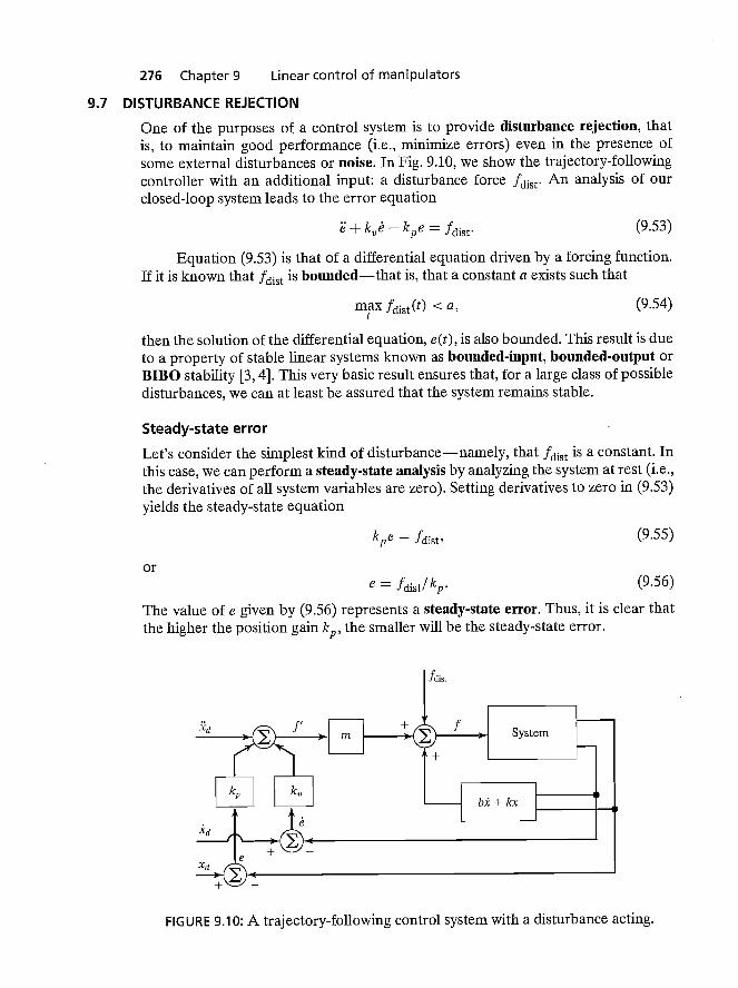
One of the purposes of a control system is to provide rejection, thatis, to maintain good performance (i.e., minimize errors) even in the presence ofsome external disturbances or noise. In Fig. 9.10, we show the trajectory-followingcontroller with an additional input: a disturbance force An analysis of ourclosed-loop system leads to the error equation

+ + = (9.53)

Equation (9.53) is that of a differential equation driven by a forcing function.If it is known that is bounded—that is, that a constant a exists such that

<a, (9.54)

then the solution of the differential equation, e(t), is also bounded. This result is dueto a property of stable linear systems known as bounded-input, bounded-output orBIIBO stability {3, 4]. This very basic result ensures that, for a large class of possibledisturbances, we can at least be assured that the system remains stable.

Steady-state error

Let's consider the simplest kind of disturbance—namely, that is a constant. Inthis case, we can perform a steady-state analysis by analyzing the system at rest (i.e.,the derivatives of all system variables are zero). Setting derivatives to zero in (9.53)yields the steady-state equation

= fthst' (9.55)

ore = fdist/kp. (9.56)

The value of e given by (9.56) represents a steady-state error. Thus, it is clear thatthe higher the position gain the smaller will be the steady-state error.

FIG U RE 9.10: A trajectory-following control system with a disturbance acting.

Section 9.8 Continuous vs. discrete time control 277

Addition of an integral term

In order to eliminate steady-state error, a modified control law is sometimes used.The modification involves the addition of an integral term to the control law. Thecontrol law becomes

= + + + k1 f edt, (9.57)

which results in the error equation

(9.58)

The term is added so that the system wifi have no steady-state error in the presenceof constant disturbances. If e(t) = 0 for t < 0, we can write (9.58) for t > 0 as

= fdist' (9.59)

which, in the steady state (for a constant disturbance), becomes

= 0, (9.60)

so

e = 0. (9.61)

With this control law, the system becomes a third-order system, and one cansolve the corresponding third-order differential equation to work out the responseof the system to initial conditions. Often, is kept quite small so that the third-ordersystem is "close" to the second-order system without this term (i.e., a dominant-pole analysis can be performed). The form of control law (9.57) is called a P11.)control law, or "proportional, integral, derivative" control law [4]. For simplicity,the displayed equations generally do not show an integral term in the control lawsthat we develop in this book.

9.8 CONTINUOUS VS. DISCRETE TIME CONTROL

In the control systems we have discussed, we implicitly assumed that the controlcomputer performs the computation of the control law in zero time (i.e., infinitelyfast), so that the value of the actuator force f is a continuous function of time. Ofcourse, in reality, the computation requires some time, and the resulting commandedforce is therefore a discrete "staircase" function. We shall employ this approximationof a very fast control computer throughout the book. This approximation is goodif the rate at which new values of f are computed is much faster than the naturalfrequency of the system being controlled. In the field of discrete time control ordigital control, one does not make this approximation but rather takes the servorate of the control system into account when analyzing the system [3].

We will generally assume that the computations can be performed quicklyenough that our continuous time assumption is valid. This raises a question: Howquick is quick enough? There are several points that need to be considered inchoosing a sufficiently fast servo (or sample) rate:


Tracking reference inputs: The frequency content of the desired or reference inputplaces an absolute lower bound on the sample rate. The sample rate must beat least twice the bandwidth of reference inputs. This is usually not the limitingfactor.

Disturbance rejection: In disturbance rejection, an upper bound on performanceis given by a continuous-time system. If the sample period is longer than thecorrelation time of the disturbance effects (assuming a statistical model forrandom disturbances), then these disturbances wifi not be suppressed. Perhapsa good rule of thumb is that the sample period should be 10 times shorter thanthe correlation time of the noise [3].

Antialiasing: Any time an analog sensor is used in a digital control scheme, therewifi be a problem with aliasing unless the sensor's output is strictly bandlimited. In most cases, sensors do not have a band limited output, and sosample rate should be chosen such that the amount of energy that appears inthe aliased signal is small.

Structural resonances: We have not included bending modes in our characterizationof a manipulator's dynamics. All real mechanisms have finite stiffness and sowifi be subject to various kinds of vibrations. If it is important to suppress thesevibrations (and it often is), we must choose a sample rate at least twice thenatural frequency of these resonances. We wifi return to the topic of resonancelater in this chapter.

9.9 MODELING AND CONTROL OF A SINGLE JOINT

In this section, we wifi develop a simplified model of a single rotary joint of amanipulator. A few assumptions wifi be made that wifi allow us to model theresulting system as a second-order linear system. For a more complete model of anactuated joint, see [5].

A common actuator found in many industrial robots is the direct current (DC)torque motor (as in Fig. 8.18). The nonturning part of the motor (the stator) consistsof a housing, bearings, and either permanent magnets or electromagnets. Thesestator magnets establish a magnetic field across the turning part of the motor (therotor). The rotor consists of a shaft and windings through which current moves topower the motor. The current is conducted to the windings via brushes, which makecontact with the commutator. The commutator is wired to the various windings (alsocalled the armature) in such a way that torque is always produced in the desireddirection. The underlying physical phenomenon [6] that causes a motor to generatea torque when current passes through the windings can be expressed as

F=qVxB, (9.62)

where charge q, moving with velocity V through a magnetic field B, experiences aforce F. The charges are those of electrons moving through the windings, and themagnetic field is that set up by the stator magnets. Generally, the torque-producingability of a motor is stated by means of a single motor torque constant, which relatesarmature current to the output torque as

= (9.63)

Section 9.9 Modeling and control of a single joint 279

When a motor is rotating, it acts as a generator, and a voltage develops across thearmature. A second motor constant, the back emf constant,3 describes the voltagegenerated for a given rotational velocity:

v = ke8i)i. (9.64)

Generally, the fact that the commutator is switching the current through various setsof windings causes the torque produced to contain some torque ripple. Althoughsometimes important, this effect can usually be ignored. (In any case, it is quite hardto model—and quite hard to compensate for, even if it is modeled.)

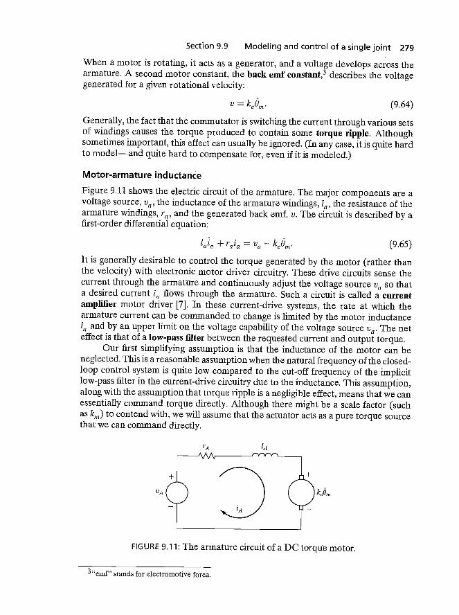
Motor-armature inductance

Figure 9.11 shows the electric circuit of the armature. The major components are avoltage source, V0, the inductance of the armature windings, the resistance of thearmature windings, ra, and the generated back emf, v. The circuit is described by afirst-order differential equation:

iota + Va — keOin. (9.65)

It is generally desirable to control the torque generated by the motor (rather thanthe velocity) with electronic motor driver circuitry. These drive circuits sense thecurrent through the armature and continuously adjust the voltage source Va 50 thata desired current flows through the armature. Such a circuit is called aamplifier motor driver [7]. In these current-drive systems, the rate at which thearmature current can be commanded to change is limited by the motor inductance1a and by an upper liniit on the voltage capability of the voltage source The neteffect is that of a low-pass filter between the requested current and output torque.

Our first simplifying assumption is that the inductance of the motor can beneglected. This is a reasonable assumption when the natural frequency of the closed-loop control system is quite low compared to the cut-off frequency of the implicitlow-pass ifiter in the current-drive circuitry due to the inductance. This assumption,along with the assumption that torque ripple is a negligible effect, means that we canessentially command torque directly. Although there might be a scale factor (suchas to contend with, we wifi assume that the actuator acts as a pure torque sourcethat we can command directly.

r11 1A

FIGURE 9.11: The armature circuit of a DC torque motor.

3"emf" stands for electromotive force.


b

FIGURE 9.12: Mechanical model of a DC torque motor connected through gearing toan inertial load.

Effective inertia

Figure 9.12 shows the mechanical model of the rotor of a DC torque motor connectedthrough a gear reduction to an inertial load. The torque applied to the rotor, tm, is

given by (9.63) as a function of the current flowing in the armature circuit. Thegear ratio (11) causes an increase in the torque seen at the load and a reduction inthe speed of the load, given by

t =

9 = (9.66)

where > 1. Writing a torque balance for this system in terms of torque at the rotoryields

= + + (1/17) (Jo + be), (9.67)

where and I are the inertias of the motor rotor and of the load, respectively, andand b are viscous friction coefficients for the rotor and load bearings, respectively.

Using the relations (9.66), we can write (9.67) in terms of motor variables as

=+ + + (9.68)

or in terms of load variables as

= (I + + (b + (9.69)

The term I + 172 is sometimes called the effective inertia "seen" at the output(link side) of the gearing. Likewise, the term b + can be called the effectivedamping. Note that, in a highly geared joint (i.e., 17 >> 1), the inertia of the motorrotor can be a significant portion of the combined effective inertia. It is this effect thatallows us to make the assumption that the effective inertia is a constant. We know

a/fl


from Chapter 6 that the inertia, I, of a joint of the mechanism actually varies withconfiguration and load. However, in highly geared robots, the variations representa smaller percentage than they would in a direct-drive manipulator (i.e., = 1). Toensure that the motion of the robot link is never underdamped, the value used for Ishould be the maximum of the range of values that I takes on; we'll call this value

This choice results in a system that is critically damped or overdamped in allsituations. In Chapter 10, we will deal with varying inertia directly and will not haveto make this assumption.

EXAMPLE 9.6

If the apparent link inertia, I, varies between 2 and 6 Kg-m2, the rotor inertia is= 0.01, and the gear ratio is = 30, what are the minimum and maximum of the

effective inertia?The minimum effective inertia is

'mm + = 2.0 + (900)(0.01) = 11.0; (9.70)

the maximum is'max + = 6.0 + (900) (0.01) = 15.0. (9.71)

Hence, we see that, as a percentage of the total effective inertia, the variation ofinertia is reduced by the gearing.

Unmodeled flexibility

The other major assumption we have made in our model is that the gearing, theshafts, the bearings, and the driven link are not flexible. In reality, all of theseelements have finite stiffness, and their flexibility, if modeled, would increase theorder of the system. The argument for ignoring flexibility effects is that, if the systemis sufficiently stiff, the natural frequencies of these unmodeled resonances are veryhigh and can be neglected compared to the influence of the dominant second-orderpoles that we have modeled.4 The term "unmodeled" refers to the fact that, forpurposes of control-system analysis and design, we neglect these effects and use asimpler dynamic model, such as (9.69).

Because we have chosen not to model structural flexibiities in the system,we must be careful not to excite these resonances. A rule of thumb [8] is that, ifthe lowest structural resonance is cores, then we must limit our closed-loop naturalfrequency according to

< (9.72)

This provides some guidance on how to choose gains in our controller. We have seenthat increasing gains leads to faster response and lower steady-state error, but wenow see that unmodeled structural resonances limit the magnitude of gains. Typicalindustrial manipulators have structural resonances in the range from 5 Hz to 25 Hz[8]. Recent designs using direct-drive arrangements that do not contain flexibility

4This is basically the same argument we used to neglect the pole due to the motor inductance.Including it would also have raised the order of the overall system.


introduced by reduction and transmission systems have their lowest structuralresonances as high as 70 Hz [9].

EXAMPLE 9.7

Consider the system of Fig. 9.7 with the parameter values in = 1, b = 1, and k = 1.

Additionally, it is known that the lowest unmodeled resonance of the system is at8 radians/second. Find a, and gains and for a position-control law so thesystem is critically damped, doesn't excite unmodeled dynamics, and has as high aclosed-loop stiffness as possible.

We choose

a = 1,

(9.73)

so that the system appears as a unit mass from the fictitious f' input. Usingour rule of thumb (9.72), we choose the closed-loop natural frequency to be

= 4 radians/second. From (9.18) and (9.46), we have = co2, so

= 16.0,

= 8.0. (9.74)

Estimating resonant frequency

The same sources of structural flexibility discussed in Chapter 8 give rise to reso-nances. In each case where a structural flexibility can be identified, an approximateanalysis of the resulting vibration is possible if we can describe the effective massor inertia of the flexible member. This is done by approximating the situation by asimple spring—mass system, which, as given in (9.20), exhibits the natural frequency

= (9.75)

where k is the stiffness of the flexible member and in is the equivalent mass displacedin vibrations.

EXAMPLE 9.8

A shaft (assumed massless) with a stiffness of 400 Nt-rn/radian drives a rotationalinertia of 1 Kg-m2. If the shaft stiffness was neglected in the modeling of thedynamics, what is the frequency of this unmodeled resonance?

Using (9.75), we have

= \/400/1 = 20 rad/second = 20/(27r)Hz 3.2 Hz. (9.76)

For the purposes of a rough estimate of the lowest resonant frequency ofbeams and shafts, [10] suggests using a lumped model of the mass. We already


0.23 in

0.33 I

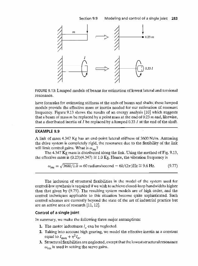
FIGURE 9.13: Lumped models of beams for estimation of lowest lateral and torsionalresonance.

have formulas for estimating stiffness at the ends of beams and shafts; these lumpedmodels provide the effective mass or inertia needed for our estimation of resonantfrequency. Figure 9.13 shows the results of an energy analysis [10] which suggeststhat a beam of mass rn be replaced by a point mass at the end of 0.23 in and, likewise,that a distributed inertia of I be replaced by a lumped 0.33 I at the end of the shaft.

EXAMPLE 9.9

A link of mass 4.347 Kg has an end-point lateral stiffness of 3600 Nt/m. Assumingthe drive system is completely rigid, the resonance due to the flexibility of the linkwifi limit control gains. What is Wres?

The 4.347 Kg mass is distributed along the link. Using the method of Fig. 9.13,the effective mass is (0.23) (4.347) 1.0 Kg. Hence, the vibration frequency is

Wres = = 60 radians/second = 60/(27r)Hz 9.6 Hz. (9.77)

The inclusion of structural flexibilities in the model of the system used forcontrol-law synthesis is required if we wish to achieve closed-loop bandwidths higherthan that given by (9.75). The resulting system models are of high order, and thecontrol techniques applicable to this situation become quite sophisticated. Suchcontrol schemes are currently beyond the state of the art of industrial practice butare an active area of research [11, 12].

Control of a single joint

In summary, we make the following three major assumptions:

1. The motor inductance 1a can be neglected.2. Taking into account high gearing, we model the effective inertia as a constant

equal to 'max +3. Structural flexibilities are neglected, except that the lowest structural resonance

is used in setting the servo gains.


With these assumptions, a single joint of a manipulator can be controlled withthe partitioned controller given by

a = 'max +

= (b + (9.78)

r=8d+kVe+kPe. (9.79)

The resulting system closed-loop dynamics are

+ + = tdjst, (9.80)

where the gains are chosen as

kP a 4 res

= = Wres. (9.81)

9.10 ARCHITECTURE OF AN INDUSTRIAL-ROBOT CONTROLLER

In this section, we briefly look at the architecture of the control system of theUnimation PUMA 560 industrial robot. As shown in Fig. 9.14, the hardware archi-tecture is that of a two-level hierarchy, with a DEC LSI-11 computer serving asthe top-level "master" control computer passing cormnands to six Rockwell 6503microprocessors.5 Each of these microprocessors controls an individual joint witha PID control law not unlike that presented in this chapter. Each joint of thePUMA 560 is instrumented with an incremental optical encoder. The encoders areinterfaced to an up/down counter, which the microprocessor can read to obtain thecurrent joint position. There are no tachometers in the PUMA 560; rather, jointpositions are differenced on subsequent servo cycles to obtain an estimate of jointvelocity. In order to command torques to the DC torque motors, the microprocessor

FIG U RE 9.14: Hierarchical computer architecture of the PUMA 560 robot-controlsystem.

5These simple 8-bit computers are already old technology. It is common these days for robotcontrollers to be based on 32-bit microprocessors.

Bibliography 285

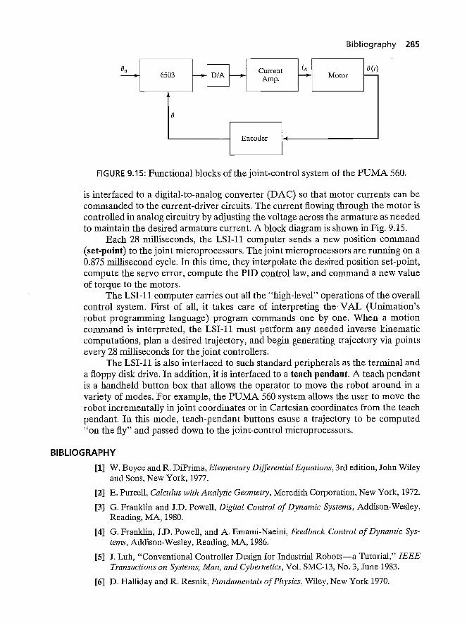
FIG U RE 9.15: Functional blocks of the joint-control system of the PUMA 560.

is interfaced to a digital-to-analog converter (DAC) so that motor currents can becommanded to the current-driver circuits. The current flowing through the motor iscontrolled in analog circuitry by adjusting the voltage across the armature as neededto maintain the desired armature current. A block diagram is shown in Fig. 9.15.

Each 28 milliseconds, the LSI-11 computer sends a new position command(set-point) to the joint microprocessors. The joint microprocessors are running on a0.875 millisecond cycle. In this time, they interpolate the desired position set-point,compute the servo error, compute the PID control law, and command a new valueof torque to the motors.

The LSI-11 computer carries out all the "high-level" operations of the overallcontrol system. First of all, it takes care of interpreting the VAL (Uriimation'srobot programming language) program commands one by one. When a motioncommand is interpreted, the LSI-11 must perform any needed inverse kinematiccomputations, plan a desired trajectory, and begin generating trajectory via pointsevery 28 miffiseconds for the joint controllers.

The LSI-11 is also interfaced to such standard peripherals as the terminal anda floppy disk drive. In addition, it is interfaced to a teach pendant. A teach pendantis a handheld button box that allows the operator to move the robot around in avariety of modes. For example, the PUMA 560 system allows the user to move therobot incrementally in joint coordinates or in Cartesian coordinates from the teachpendant. In this mode, teach-pendant buttons cause a trajectory to be computed"on the fly" and passed down to the joint-control microprocessors.

BIBLIOGRAPHY

[1] W. Boyce and R. DiPrima, Elenwntary Differential Equations, 3rd edition, John Wileyand Sons, New York, 1977.

[2] E. Purcell, Calculus with Analytic Geometry, Meredith Corporation, New York, 1972.

[3] G. Franklin and J.D. Powell, Digital Control of Dynamic Systems, Addison-Wesley,Reading, MA, 1980.

[4] G. Franklin, J.D. Powell, and A. Emami-Naeini, Feedback Control of Dynamic Sys-tems, Addison-Wesley, Reading, MA, 1986.

[5] J. Luh, "Conventional Controller Design for Industrial Robots—a Tutorial," IEEETransactions on Systems, Man, and Cybernetics, Vol. SMC-13, No. 3, June 1983.

[6] D. Haffiday and R. Resnik, Fundamentals of Physics, Wiley, New York 1970.


[7] Y. Koren and A. Ulsoy, "Control of DC Servo-Motor Driven Robots," Proceedingsof Robots 6 Conference, SIvifi, Detroit, March 1982.

[8] R.P. Paul, Robot Manipulators, MIT Press, Cambridge, MA, 1981.

[9] H. Asada and K. Youcef-Toumj, Direct-Drive Robots—Theory and Practice, MITPress, Cambridge, MA, 1987.

[10] J. Shigley, Mechanical Engineering Design, 3rd edition, McGraw-Hill, New York, 1977.

[11] W. Book, "Recursive Lagrangian Dynamics of Flexible Manipulator Arms," TheInternational Journal of Robotics Research, Vol. 3, No. 3, 1984.

[12] R. Cannon and E. Sclmiitz, "Initial Experiments on the End-Point Control of aFlexible One Link Robot," The International Journal of Robotics Research, Vol. 3,No. 3, 1984.

[13] R.J. Nyzen, "Analysis and Control of an Eight-Degree-of-Freedom Manipulator,"Ohio University Master's Thesis, Mechanical Engineering, Dr. Robert L. Wffliams II,Advisor, August 1999.

[14] R.L. Williams II, "Local Performance Optimization for a Class of Redundant Eight-Degree-of-Freedom Manipulators," NASA Technical Paper 3417, NASA LangleyResearch Center, Hampton, VA, March 1994.

EXERCISES

9.1 [20] For a second-order differential equation with complex roots

= —

show that the general solution

x(t) = + c9eS2t,

can be writtenx(t) = c1eAt cos(jst) + c2eAt

9.2 [13] Compute the motion of the system in Fig. 9.2 if parameter values are in = 2,b = 6, and k = 4 and the block (initially at rest) is released from the positionx =1.



9.5 [15] Compute the motion of the system in Fig. 9.2 if parameter values are in = 1,b = 7, and k = 10 and the block is released from the position x = 1 with an initialvelocity of x = 2.

9.6 [15] Use the (1, 1) element of (6.60) to compute the variation (as a percentageof the maximum) of the inertia "seen" by joint 1 of this robot as it changesconfiguration. Use the numerical values

= 12 0.5 m,

in1 = 4.0 Kg,

ifl2 =2.0Kg.

Programming exercise (Part 9) 287

Consider that the robot is direct drive and that the rotor inertia is negligible.9.7 [17] Repeat Exercise 9.6 for the case of a geared robot (use = 20) and a rotor

inertia of = 0.01 Kg m2.9.8 [18] Consider the system of Fig. 9.6 with the parameter values in = 1, b = 4,

and k = 5. The system is also known to possess an unmodeled resonance atWres = 6.0 radians/second. Determine the gains and that will critically dampthe system with as high a stiffness as is reasonable.

9.9 [25] In a system like that of Fig. 9.12, the inertial load, I, varies between 4 and5 Kg-rn2. The rotor inertia is = 0.01 Kg-rn2, and the gear ratio is = 10.

The system possesses uninodeled resonances at 8.0, 12.0, and 20.0 radians/second.Design a and fi of the partitioned controller and give the values of and suchthat the system is never underdamped and never excites resonances, but is as stiffas possible.

9.10 [18] A designer of a direct-drive robot suspects that the resonance due to beamflexibility of the link itself will be the cause of the lowest unmodeled resonance. Ifthe link is approximately a square-cross-section beam of dimensions 5 x 5 x 50 cmwith a 1-cm wall thickness and a total mass of 5 Kg, estimate cores.

9.11 [15] A direct-drive robot link is driven through a shaft of stiffness 1000 Nt-rn/radian.The link inertia is 1 Kg-m2. Assuming the shaft is massless, what is Wres?

9.12 [18] A shaft of stiffness 500 Nt-mlradian drives the input of a rigid gear pair with1) = 8. The output of the gears drives a rigid link of inertia 1 Kg-rn2. What is theC0res caused by flexibility of the shaft?

9.13 [25] A shaft of stiffness 500 Nt-rn/radian drives the input of a rigid gear pair with= 8. The shaft has an inertia of 0.1 Kg-rn2. The output of the gears drives a rigid

link of inertia 1 Kg-rn2. What is the Wres caused by flexibility of the shaft?9.14 [28] In a system like that of Fig. 9.12, the inertial load, I, varies between 4 and

5 Kg-rn2. The rotor inertia is = 0.01 Kg-rn2, and the gear ratio is = 10. Thesystem possesses an unmodeled resonance due to an end-point stiffness of thelink of 2400 Nt-rn/radian. Design a and fi of the partitioned controller, and givethe values of and k0 such that the system is never underdamped and neverexcites resonances, but is as stiff as possible.

9.15 [25] A steel shaft of length 30 cm and diarneter 0.2 cm drives the input gear of areduction of 17 = 8. The rigid output gear drives a steel shaft of length 30 cm anddiameter 0.3 cm. What is the range of resonant frequencies observed if the loadinertia varies between 1 and 4 Kg-rn2?

PROGRAMMING EXERCISE (PART 9)

We wish to simulate a simple trajectory-following control systern for the three-link planararrn. This control system will be implemented as an independent-joint PD (proportionalplus derivative) control law. Set the servo gains to achieve closed-loop stiffnesses of175.0, 110.0, and 20.0 for joints 1 through 3 respectively. Try to achieve approximatecritical damping.

Use the simulation routine UPDATE to simulate a discrete-time servo runningat 100 Hz—that is, calculate the control law at 100 Hz, not at the frequency of thenumerical integration process. Test the control scheme on the following tests:

1. Start the arm at 0 = (60, —110, 20) and command it to stay there until time = 3.0,when the set-points should instantly change to 0 = (60, —50, 20). That is, give astep input of 60 degrees to joint 2. Record the error—time history for each joint.

2. Control the arm to follow the cubic-spline trajectory from Programming ExercisePart 7. Record the error—time history for each joint.


MATLAB EXERCISE 9

This exercise focuses on linearized independent joint-control simulation for the shoulderjoint (joint 2) of the NASA eight-axis AAI ARJVIII (Advanced Research Manipulator II)manipulator arm—see [14]. Familiarity with linear classical feedback-control systems,including block diagrams and Laplace transforms, is assumed. We will use Simulink, thegraphical user interface of MATLAB.

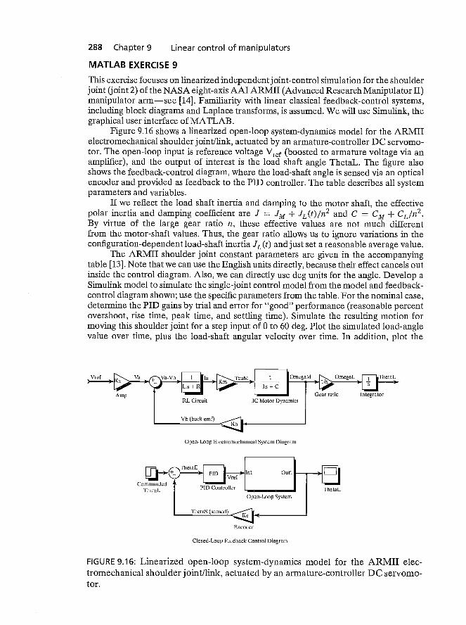
Figure 9.16 shows a linearized open-loop system-dynamics model for the ARMIIelectromechanical shoulder joint/link, actuated by an armature-controller DC servomo-tor. The open-loop input is reference voltage (boosted to armature voltage via anamplifier), and the output of interest is the load shaft angle ThetaL. The figure alsoshows the feedback-control diagram, where the load-shaft angle is sensed via an opticalencoder and provided as feedback to the PTD controller. The table describes all systemparameters and variables.

If we reflect the load shaft inertia and damping to the motor shaft, the effectivepolar inertia and damping coefficient are J = + JL(t)/n2 and C = CM + CL/n2.By virtue of the large gear ratio n, these effective values are not much differentfrom the motor-shaft values. Thus, the gear ratio allows us to ignore variations in theconfiguration-dependent load-shaft inertia (t) and just set a reasonable average value.

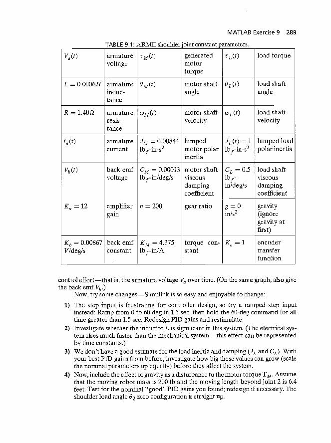
The ARJVHI shoulder joint constant parameters are given in the accompanyingtable [13]. Note that we can use the English units directly, because their effect cancels outinside the control diagram. Also, we can directly use deg units for the angle. Develop aSimulink model to simulate the single-joint control model from the model and feedback-control diagram shown; use the specific parameters from the table. For the nominal case,determine the PID gains by trial and error for "good" performance (reasonable percentovershoot, rise time, peak time, and settling time). Simulate the resulting motion formoving this shoulder joint for a step input of 0 to 60 deg. Plot the simulated load-anglevalue over time, plus the load-shaft angular velocity over time. In addition, plot the

CommandedmetaL

Encoder

Closed-Loop Feedback Control Diagram

FIGURE 9.16: Linearized open-loop system-dynamics model for the ARMII elec-tromechanical shoulder joint/link, actuated by an armature-controller DC servomo-tor.

Door rotio Integrator

Open-Loop Electromechanieal System Diagrom

MATLAB Exercise 9 289

TABLE 9.1: ARMII shoulder loirit constant parameters.

Va(t) armaturevoltage

-rM(t) generatedmotortorque

TL(t) load torque

L = 0.0006H armatureinduc-tance

9M(t) motor shaftangle

OL(t) load shaftangle

R = 1.40Q armatureresis-tance

coM(t) motor shaftvelocity

WL(t) load shaftvelocity

(t) armaturecurrent

= 0.00844lbf -in-s2

lumpedmotor polarinertia

(t) = 1

lbf -in-s2lumped loadpolar inertia

Vb (t) back emfvoltage

CM = 0.00013lbf-in/deg/s

motor shaftviscousdampingcoefficient

CL = 0.5

lbf-in/deg/s

load shaftviscousdampingcoefficient

= 12 amplifiergain

n = 200 gear ratio g = 0

in/s2gravity(ignoregravity atfirst)

Kb = 0.00867V/deg/s

back emfconstant

KM = 4.375lbf -in/A

torque con-stant

= 1 encodertransferfunction

control effort—that is, the armature voltage Va over time. (On the same graph, also givethe back emf Vb.)

Now, try some changes—Simulink is so easy and enjoyable to change:

1) The step input is frustrating for controller design, so try a ramped step inputinstead: Ramp from 0 to 60 deg in 1.5 sec, then hold the 60-deg command for alltime greater than 1.5 sec. Redesign PID gains and restimulate.

2) Investigate whether the inductor L is significant in this system. (The electrical sys-tem rises much faster than the mechanical system—this effect can be representedby time constants.)

3) We don't have a good estimate for the load inertia and damping and CL). Withyour best PID gains from before, investigate how big these values can grow (scalethe nominal parameters up equally) before they affect the system.

4) Now, include the effect of gravity as a disturbance to the motor torque TM. Assumethat the moving robot mass is 200 lb and the moving length beyond joint 2 is 6.4feet. Test for the nominal "good" PID gains you found; redesign if necessary. Theshoulder load angle 87 zero configuration is straight up.

linear control of manipulators

Documents