1

Liquidity tail risk and the implied cost of equity capital

September 2016

Abstract

We examine the relationship between liquidity tail risk and the implied cost of capital for firms

from 46 countries. We document robust evidence that firms whose stocks have larger liquidity tail

risk suffer from higher cost of capital. A one standard deviation increase in liquidity tail risk leads

to a rise of 35 basis points in the cost of equity. We further find that this relation is stronger in

periods of down markets and high volatility. Moreover, we show that better information quality

and stronger investor protection mitigate the effect of liquidity tail risk on the cost of capital.

JEL classification: G11; G12; G14; G15; F36

Keywords: Liquidity; Tail risk; Cost of capital; Market conditions; Institutions

2

1. Introduction

Stock liquidity is of particular concern to investors. Extant literature on stock liquidity and

expected returns has mainly focused on two liquidity properties: mean (liquidity level) and

variability (liquidity risk). Amihud and Mendelson (1986) show that investors prefer liquid stocks

that allow large trades with least transaction costs and provide empirical evidence that expected

returns decrease in the level of liquidity. Independent of the level of liquidity, later research shows

that the time-varying nature of liquidity constitutes a source of risk that also has an impact on stock

returns (e.g., Pastor and Stambaugh, 2003; Sadka, 2006; and Acharya and Pedersen, 2005).

Though extensive, prior literature has largely overlooked another liquidity property that can

potentially influence expected returns, namely liquidity tail risk. In this paper, we aim to bridge

this gap in the literature by conducting a thorough investigation of the relation between liquidity

tail risk and a stock’s expected returns.

We address the issue of whether investors require a compensation for bearing extreme

liquidity risk1 that is specific to a given security, defined as the potential for an individual stock’s

liquidity costs to exceed a certain threshold. This is an important question especially that a stock

is in a normal liquidity state most of the time but is occasionally subject to episodes where its

liquidity suddenly vanishes, making it extremely costly for traders to enter or exit positions.

Practitioners are fully aware of the risk of sharp declines in liquidity wherein trades may fail to

occur because of the lack of counterparties on the other side. The importance of focusing on the

tail of liquidity rather than on its level was emphasized in a recent comment by the Financial Times

1 Throughout this paper, we use the terms “extreme liquidity risk” and “liquidity tail risk” interchangeably to designate the potential for a stock’s

liquidity to fall below a certain threshold.

3

chief economics commentator, Martin Wolf, on the findings of the IMF’s 2015 Global Financial

Stability report. He states, “The big problem with such analyses is that things tend to look fine

until they do not. One has to focus instead on the tail risks…Investors ought to worry, instead,

since the risk that nobody will be on the other side of their trades is a real one.” (FT, Oct. 6, 2015).

Despite such calls on the importance of liquidity tails, there is only limited empirical research that

investigates the impact of infrequent, but severe, liquidity drops on expected returns. In this paper,

we contribute to this literature by investigating the relation between stock extreme liquidity risk

and the implied cost of equity capital in a cross-country setting and further assess the extent to

which it is affected by market conditions and country institutional factors.

The fear that a stock’s liquidity can suddenly evaporate may have a significant influence

on the price that investors are willing to pay. In a recent paper, Ang et al. (2014) argue that the

infrequent and rather unexpected liquidity dry-ups expose investors to liquidity crises and increase

their propensity to pay a significant risk premium to avoid illiquidity. Ang et al. (2014: p. 2,738)

suggest that their model is “applicable to a wide range of assets that are normally liquid, but are

subject to occasional market freezes”. Pertinent to the stock market, Ang et al. (2014)’s theory

predicts that stock extreme liquidity risk varies across stocks and that investors may be more

concerned about holding stocks with higher extreme liquidity risk. Intuitively, traders may be

reluctant to supply liquidity for extremely illiquid stocks lest they are trapped in positions waiting

for the arrival of an eventual buyer or having to incur very high trading costs. In exchange for

providing immediacy, these traders would charge a discount and require larger price concessions

to enter positions on such stocks, which translates into a higher cost of equity capital. Inversely,

firms with a lower tendency to experience liquidity crashes should enjoy cheaper cost of equity as

investors are willing to pay more for shares that trade at any time without suffering major losses.

4

To assess stock extreme liquidity risk we focus on the tail distribution of an individual

stock’s liquidity measured by the Amihud (2002) proxy. We adopt Extreme Value Theory, which

deals with extreme behavior of a probability distribution. Extreme Value Theory models the

behavior of heavy tailed distributions and provides the best possible estimate of the tail index of

the distribution.2 We apply the parametric Maximum Likelihood Estimation approach on

Generalized Pareto Distribution to gauge the liquidity tail index (𝐿𝑇𝐼 hereafter) and use it as our

primary measure of liquidity tail risk. The liquidity tail index captures the potential exceedances

of an individual stock’s illiquidity over a certain threshold. It is thus a measure of tail risk in stock

liquidity in the spirit of Wu (2015). While Wu (2015) uses this threshold-based measure to estimate

the frequency of market-wide extreme liquidity events, we rather focus on the tail distribution of

liquidity at the stock level. In Wu’s (2015) empirical analysis, extreme liquidity risk refers to the

sensitivity of a stock’s return to market-wide extreme liquidity events whereas in our analysis it

refers to the potential for a stock’s liquidity to spiral down below a certain threshold. In this regard,

our approach to extreme liquidity risk is closer to Menkveld and Wang (2012) who study whether

liquileaks, defined as the probability that a stock hits an illiquid state and remains in that state for

a week or longer, affects expected returns. However, unlike Menkveld and Wang (2012) our

measure of extreme liquidity risk captures the potential for a stock’s illiquidity to exceed a certain

threshold rather than the probability to be trapped in an illiquid state for a certain period of time.

Our paper also differs from Menkveld and Wang (2012) in two other major aspects. First,

while they focus on the U.S. equity market, we use an international setting that encompasses stocks

from different markets with various institutional characteristics. Our international setting offers

2There is a substantial literature that has modeled extremes using jump processes (e.g., Duffie et al., 2000) and copulas (e.g., Ruenzi et al., 2013).

5

the advantage of capturing the potentially wide variation in stock extreme liquidity risk across

countries. Indeed, little is known about the extent to which stocks are prone to severe liquidity dry-

ups in countries other than the U.S and whether this determines firms’ cost of capital. By taking a

global approach, this paper exploits the rich variation in the nature of equity markets and considers

markets where stock liquidity may be particularly fragile and where investors’ concern for such

severe fragility may be particularly strong. This setting allows us to provide a better understanding

of the nature of the relation between extreme liquidity risk and firm cost of capital. Second, as a

measure of expected returns, Menkveld and Wang (2012) use realized returns while we use the

cost of equity implied by the stock price and earnings forecasts (𝑅𝐼𝐶𝐶) known to be a better proxy

for expected returns. Pastor et al. (2008) empirically show that the implied cost of capital

outperforms realized returns in detecting a risk– return tradeoff.3 They further recommend using

𝑅𝐼𝐶𝐶 rather than realized returns because the former is forward-looking with greater capacity to

capture the time-varying expected returns. Li et al. (2013) show that 𝑅𝐼𝐶𝐶 has a greater ability than

traditional ratios in predicting future stock returns. Botosan and Plumlee (2005), Chava and

Purnanandam (2010), and Botosan et al. (2011) also support the use of 𝑅𝐼𝐶𝐶 as a proxy of expected

returns.

To further investigate the relation between extreme liquidity and the cost of capital, we

assess the potential influence of market conditions. While investors’ concern about the potential

for a stock’s liquidity to dry-up is continuous, it can be even more acute in periods of market

turmoil. This is justified by the fact that stock liquidity behaves differently in normal periods versus

3 Prior studies advocate the use of the implied cost of equity capital as a measure of expected returns by investors (e.g., Claus and Thomas, 2001;

Gebhardt et al., 2001; Easton, 2004; Ohlson and Juettner, 2005). Yet, most of the literature examining the relation between liquidity and stock

prices uses ex post realized returns as a proxy for expected returns (e.g., Brennan and Subrahmanyam, 1996; Amihud, 2002; Datar et al., 1998;

Brennan et al., 1998; Asparouhova et al., 2010; Brennan et al., 2012; Bali et al., 2014). Realized returns are, however, said to be poor proxies of expected returns (e.g., Elton, 1999; Easton and Monahan, 2005; Lunbland, 2007).

6

crisis periods when markets are characterized by low returns or high volatility. Early empirical

research has documented this asymmetric behavior of stock liquidity. For instance, Pastor and

Stambaugh (2003) report a much higher correlation between stock liquidity and market returns

(0.5) in negative-return months compared to positive-return months (near zero). Recent theoretical

research also suggests that sudden liquidity dry-ups occur more during market downturns and

increased volatility. The theoretical model of Brunnermeier and Pederson (2009) predicts that

financial market turmoil tightens funding constraints of traders and thereby lowers their ability to

provide liquidity. When markets decline, traders suffer losses on securities they use as collateral

or face greater margins, which leads them to provide less liquidity and liquidate their positions in

many securities. This reduced market liquidity leads to more losses and higher margins, creating

an “illiquidity spiral” that further lowers traders’ ability to provide liquidity. The theories in Gromb

and Vayanos (2002) and Kyle and Xiong (2001) also suggest that an increased volatility tightens

traders’ funding constraints which restrict their capacity to provide liquidity. A common theme

among these studies is that liquidity tends to evaporate in times of high volatility or declines in

financial markets. Stocks’ potential to fall into extreme liquidity states thus increases during

market turmoil which may affect investors’ expected returns. Motivated by these studies, we

investigate whether the relation between stock extreme liquidity risk and the implied cost of equity

is influenced by market conditions. Our conjecture is that the impact of extreme liquidity risk on

the cost of equity is more pronounced in crisis periods. In other words, investors pay lower prices

for stocks with higher extreme liquidity risk, but more so in periods of market decline and high

volatility.

In our last analysis, we study whether the varying institutional environments across our

sample countries influence the documented relation between extreme liquidity risk and the implied

7

cost of capital. A growing body of literature on liquidity highlights the importance of country-level

institutional quality on stock liquidity level and risk. Information quality and investor protection

are two institutional traits that have been particularly shown to play a significant role in enhancing

equity markets’ liquidity. Regarding information quality, countries that emphasize greater

transparency and disclosure by firms mitigate information asymmetry and reduce investors’

uncertainty about the intrinsic value of stocks, which potentially leads to higher liquidity level and

lower liquidity risk.4 Consistent with this argument, Eleswarapu and Venkataraman (2006) report

evidence that stocks from countries with better accounting standards enjoy lower liquidity costs.

As for liquidity risks, Dang et al. (2015) report evidence of higher commonality in liquidity in

countries with more information opacity. Moreover, the extent to which a country provides legal

protection to investors can also affect liquidity through its impact on information quality and

investor participation. Empirical evidence suggests that stronger investor protection lowers a

stock’s cost of liquidity (Eleswarapu and Venkataraman, 2006) and that liquidity commonality is,

on average, higher in countries with poor investor protection (Karolyi et al., 2012; Dang et al.,

2015). While these studies document the effect of information quality and investor protection on

liquidity level and risk, no prior research has examined the interaction between these institutional

factors, extreme liquidity risk, and the cost of capital. We fill this gap in the literature by

investigating whether the strength of the relation between extreme liquidity risk and the cost of

capital varies across countries according to the level of investor protection and information quality.

4 Market microstructure models, such as Copeland and Galai (1983), Glosten and Milgrom (1985), and Kyle (1985) predict a negative relation

between information asymmetry and stock liquidity because the likelihood of informed trading raises the cost of market making by market makers. More recent theoretical models, such as Vayanos (2004) and Brunnermeier and Pedersen (2009) show that liquidity can dry-up due to a “flight to

quality”, where liquidity providers exit positions on assets who present high levels of uncertainty about their intrinsic value. Lang and Maffet (2011:

p.102) argue that “to the extent that transparency provides information about, for example, future cash flows, it reduces uncertainty about intrinsic value, potentially reducing the sensitivity of liquidity to market shocks”.

8

Specifically, we expect that investors should be more concerned about extreme liquidity risk in

environments characterized by more information opacity and weaker investor protection.

We conduct our analysis of the relation between extreme liquidity risk and the cost of equity

capital in an international sample consisting of 14,702 different stocks from 46 countries over the

period spanning 1985 to 2012 (more than 100,000 observations). Our results suggest that extreme

liquidity risk is a component of the firm cost of equity beyond liquidity level and co-variance risks,

while controlling for firm- and country-level determinants. Our findings indicate that a one

standard deviation increase in 𝐿𝑇𝐼 raises 𝑅𝐼𝐶𝐶 by 35 basis points. This result is robust to the use of

alternative proxies of extreme liquidity risk: Hill’s (1975) tail index estimator, liquidity black hole

(LBH) defined as the frequency of extreme illiquidity incidences, and liquidity kurtosis. The

reported evidence that firms with higher liquidity tail risk bear more expensive cost of equity

capital on an ex-ante basis is novel and survives a battery of robustness tests including, the use of

alternative measures of 𝑅𝐼𝐶𝐶, noise in the analyst forecasts, bias in sample selection, and the

introduction of additional control variables. We further find that the adverse effect of extreme

liquidity risk on the implied cost of capital is more severe during episodes of market downturns

and higher market volatility, suggesting that investors become more concerned about holding

stocks with larger extreme liquidity risk in periods of market turmoil. Our empirical evidence also

points to the importance of institutional environments to the relation between extreme liquidity

risk and the cost of capital. Specifically, we find that better information quality and stronger

investor protection mitigate the influence of liquidity tail risk on the cost of capital.

Our study contributes to several strands of the literature. First, we add to the important yet

scant literature on extreme liquidity risk. Existing studies are few and typically examine the

9

potential impact of a stock’s sensitivity to market-wide liquidity crashes on realized stock returns

(Ruenzi et al., 2013; Anthonisz and Puntins, 2016; and Wu, 2015). By focusing on extreme

liquidity risk that is specific to an individual stock, we rather allow for the cost of equity to be

potentially determined by a liquidity risk other than just the linear co-variation between stock

liquidity and market liquidity and returns – the risk that liquidity spirals down below a certain

threshold to extremely low levels.5 Using a new measure of extreme liquidity risk, the implied cost

of equity, and an international setting, we provide several new insights on extreme liquidity risk.

We primarily document robust evidence that extreme liquidity risk requires an equity premium

globally. We further show that the magnitude of this premium increases in times of market

downturns and higher volatility. Moreover, we report that the extent to which investors are

concerned about extreme liquidity risk varies across countries according to their institutional

quality, especially the quality of information and investor protection.

Second, our work adds to the literature that examines liquidity in international markets. The

findings of Lee (2011), Karolyi et al. (2012), and Amihud et al. (2015) suggest that stock liquidity

level and risk are priced differently across countries according to geographic, economic, and

institutional environments. We add to these studies by focusing on a different dimension of

liquidity, namely the potential for a stock’s liquidity to dry-up. To the best of our knowledge, this

is the first study that addresses this issue in an international setting. We complement the findings

of the above literature with evidence that extreme liquidity risk matters to investors in international

5 There is a vast theoretical and empirical literature on liquidity. Recent studies include Pastor and Stambaugh (2003), Acharya and Pedersen

(2005), Sadka (2006), Bekaert et al. (2007), Watanabe and Watanabe (2008), Kamara et al. (2008), Koch et al. (2016), Brunnermeier and Pedersen (2009), Hameed et al. (2010), Lee (2011), Ng (2011), Nagel (2012), Karolyi et al. (2012), and Amihud et al. (2015).

10

financial markets with an impact on the cost of equity that varies by financial market conditions

and by the quality of countries’ institutional environments.

Third, our paper contributes to a growing body of literature on rare events that stresses the

importance of extreme event risk as a factor to be accounted for in models that explain properties

of equity returns. Two early studies by Mandelbrot (1963) and Fama (1965) document that the

distribution of US stock returns have univariate heavy tails. More recently, Kelly and Jiang (2014)

study the effects of extreme event risk in stock markets and provide evidence of a tail risk

premium: an increase in the tail risk of returns has a positive impact on future stock returns.

Consistent with extreme event risk being priced, Chabi-Yo et al. (2015) and Gao and Song (2015)

find that stocks that are more sensitive to tail risk earn higher returns. Bollerslev and Todorov

(2011) report empirical results showing that the way in which the stock market generally prices

risky payoffs incorporates the possible occurrence of rare disasters, and that the fear of such events

accounts for a large fraction of the historically observed equity risk premia. We add to this

literature by showing that apart from extreme return risk, extreme liquidity risk is also a significant

determinant of firms’ cost of equity capital.

Fourth, our paper contributes to the literature on the determinants of the cost of equity capital.

Prior cross-country studies suggest that the implied cost of capital is influenced by the nature of a

country’s institutions (e.g., Hail and Leuz, 2006) and several firm-level factors, such as voluntary

disclosure (Francis et al., 2005) and corporate governance (e.g., Chen et al., 2011). While these

studies generally underscore the importance of firm-level characteristics for the implied cost of

equity, none of them considers the potential association between extreme liquidity risk and the

implied cost of capital for international firms. We thus extend the cost of capital literature by

11

providing novel evidence that extreme liquidity risk is a significant determinant of the cost of

equity.

Our findings on extreme liquidity risk and cost of capital have several important

implications. First, our findings suggest that investors require a greater compensation for holding

stocks whose liquidity has a greater tendency to spiral down, which translates into a higher cost of

capital and a lower firm valuation, all else being equal. This evidence suggests that firms can enjoy

cheaper cost of capital and higher valuation by putting in place policies that would enhance stocks’

liquidity and reduce its potential to reach extremely low levels. One potential measure is to enhance

disclosure, which according to Balakrishnan et al. (2014) improves stock liquidity and thereby

reduces firm cost of capital. Also, our empirical evidence has public policy implications. The

findings that the extreme liquidity risk premium is higher in environments with better information

quality and investor protection suggest that certain countries with poor records along these two

institutional dimensions can contribute to the lowering of their firms’ cost of capital by adopting

reforms aimed at strengthening investor protection and reducing information opaqueness. Such

measures would lower firms’ cost of capital, increase investment and job creation, which are much

needed in many countries.

The remainder of the paper is organized as follows. Section 2 describes our data and

variables. Section 3 presents our empirical results. Finally, section 4 concludes.

2. Data and variables

2.1. Sample selection and data filtering

We extract all available equities listed on all stock exchanges around the world from

DataStream, for the period spanning January 1985 to October 2012. To maximize the stock

12

coverage of our study, we include all exchanges within any single country.6 We remove depositary

receipts (DRs), real estate investment trusts (REITs), preferred stocks, investment funds, iShares,

mutual funds, municipal funds, 144A, and stocks with special features. In some countries, we apply

specific filters to discard preferred stocks, income trusts, and non-common stocks.7

For every stock within our sample, we collect the daily total return index (RI), the daily trading

volume (VO), the daily price in local currency (P), and the market capitalization in US dollars

(MV). We exclude non-trading days, which we identify, for a given exchange, as days in which

more than 90% of the listed stocks have zero returns. We also exclude stock-months for which the

number of zero-return days in a certain month exceeds 80%. We set daily returns to missing if the

value of the total return index for either the previous or the current day is below 0.01. Following

Ince and Porter (2006), we fix errors in Datastream data reporting by setting daily returns to

missing if a daily return equals or exceeds 100% and is reversed the following day. In other words,

the daily returns for both days d and d-1 are set to missing if 𝑟𝑑𝑖 × 𝑟𝑑−1

𝑖 − 1 ≤ 0.5, where 𝑟𝑑𝑖 is the

gross return for stock 𝑖 on day d, and at least one of the two returns is 200% or greater. We further

impose a price restriction where stocks with year-end prices that fall within the bottom or top 2.5%

percentile range of the cross section for a given country are excluded from the sample in the

6 For instance, we include Shanghai and Shenzen exchanges for China, Osaka and Tokyo stock exchanges for Japan, and Nasdaq, NYSE, and

NYSE MKT LLC stock exchanges for the U.S. 7 Following Karolyi et al. (2012), we extract all available equities in Datastream, including active, dead, and suspended, to eliminate the survivorship

bias. To eliminate depositary receipts (DRs), real estate investment trusts (REITs), preferred stocks, investment funds, iShares, mutual funds,

municipal funds, 144A, or other stocks with special features, we exclude stocks whose names include “REIT”, “REAL EST”, “GDR”, “PF”,

“PREF”, or “PRF” as these terms may represent REITs, GDRs, or preferred stocks. We also exclude stocks whose names include “ADS”, “RESPT”, “UNIT”, “TST”, “TRUST”, “INCOME FD”, “INCOME FUND”, “UTS”, “RST”, “CAP.SHS”, “INV”, “HDG”, “SBVTG”, “VTG.SAS”,

“GW.FD”, “RTN.INC”, “VCT”, “ORTF”, “HI.YIELD”, “PARTNER”, ”HIGH INCOME”, “INC.&GROWTH”, “INC.&GW”, "%", "DOW

JONES", "ISHARE", "FD.UNT", "MERGER", "MUT FUND", "PRTF", "MUN.FD", "144A", "INSD. FD", "INSD.FD", "INSD", "MSDW", "MRLY", "MGST", "MERR.LYNCH", "LEHMAN BROS", "MUN.BD", and "CAP.TAX". We exclude stocks whose sector is "Real Estate

Investment Trusts". Further, we apply the following additional country-specific stock filers. In Belgium, we discard stocks whose names include

“AFV” and “VVPR”. In Brazil, we exclude preferred stocks whose names contain “PN”. In Canada, we exclude income trusts by removing stocks with names including “INC.FD.”. In Mexico, we discard convertible shares of the types “ACP” and “BCP”. In France, we exclude preferred shares

whose names include “ADP” and “CIP”. In Germany, we exclude preferred shares with names including “GSH”. In Italy, we discard non-voting

shares with names including “RSP”. In the U.S., we exclude ADRs by examining the names of stocks and non-common stocks by checking the CUSIP. We only include U.S. common shares whose 7th and 8th digits of the CUSIP are 1 and 0, respectively.

13

following year. Finally, we require each stock to have a valid market capitalization in US dollars

at the end of each year.

2.2. Main variables

2.2.1. The implied cost of equity capital

Recent literature advocates the ex-ante cost of equity implied by stock prices and analysts’

earnings forecasts as a better measure of expected returns than the ex-post returns (e.g., Hail and

Leuz, 2006; Pastor et al., 2008). According to Pastor et al. (2008, p. 2860), “One appealing feature

of the ICC [Implied cost of capital] as a proxy for expected returns is that it does not rely on noisy

realized asset returns”.

We follow Hail and Leuz (2006) and Dhaliwal et al. (2006) and calculate the implied cost

of capital, 𝑅𝐼𝐶𝐶, as the average estimate obtained from four different models, Claus and Thomas

(2001), Gebhardt et al. (2001), Easton (2004), and Ohlson and Juettner-Nauroth (2005). Using the

average of four estimates has the advantage of reducing the possibility of obtaining biased results

due to the reliance on one model rather than the others (Dhaliwal et al., 2006). The individual

estimates of the implied cost of capital obtained using the models of Claus and Thomas (2001),

Gebhardt et al. (2001), Easton (2004), and Ohlson and Juettner-Nauroth (2005) are denoted 𝑅𝐶𝑇,

𝑅𝐺𝐿𝑆, 𝑅𝐸𝑆, 𝑅𝑂𝐽𝑁 respectively. We note that 𝑅𝑂𝐽𝑁 is estimated in a closed form solution while 𝑅𝐶𝑇,

𝑅𝐺𝐿𝑆, and 𝑅𝐸𝑆 involve numerical techniques wherein the solution is bounded between 0% and

100%.

To calculate 𝑅𝐼𝐶𝐶, we use I/B/E/S database to get the positive one-, two-, and three- year-

ahead mean forecasted earnings per share (𝐹𝐸𝑃𝑆𝑡+𝑗) and the long-term growth rate forecast. In

line with Frankel and Lee (1998) and Hail and Leuz (2009), we substitute missing or negative

14

𝐹𝐸𝑃𝑆𝑡+𝑗 by the historical earnings per share estimated using the beginning year book value per

share and the three-year median return on equity in the same year, country, and industry. In this

study, we consider only firms with sufficient I/B/E/S forecasts. We eliminate firm-year

observations for which none of the implied cost of equity estimates converges (Easton, 2004; Claus

and Thomas, 2001; and Gebhardt et al., 2001 models) or is undefined (Ohlson and Juettner-

Nauroth, 2005 model).8 We provide detailed descriptions of the four models used to estimate the

implied cost of equity in Appendix A.

2.2.2. Amihud liquidity proxy

Following recent international studies on liquidity, such as Amihud et al. (2015), we rely

on the widely used liquidity proxy developed by Amihud (2002). Amihud (2002) liquidity measure

reflects the price impact of a monetary unit of trade. According to this measure a stock is

considered liquid if it can accommodate heavy trading with the least impact on the price. Two

characteristics contribute to the popularity of the Amihud measure. First, it has the advantage of

having a simple construction that uses the absolute value of the daily return-to-volume ratio to

capture price impact. It is thereby easy to calculate, especially in markets suffering from data

limitations, which makes it a suitable proxy for liquidity in studies of liquidity covering

international samples. Second, it exhibits strong positive correlation with Kyle’s (1985)

microstructure estimate of the price impact measure. Using U.S. data, Hasbrouck (2009) shows

that the Amihud measure is more correlated with high-frequency price impact coefficient than any

other daily liquidity proxy. The Amihud measure is also shown to have high correlation with bid-

8 In a robustness test, we impose the restriction of having a valid cost of equity estimate for each model before taking the average to calculate 𝑅𝐼𝐶𝐶.

The results remain unchanged.

15

ask spreads in emerging markets (Lesmond, 2005). Fong et al. (2014) confirm the suitability of

Amihud (2002) illiquidity measure for international liquidity studies by reporting that, across

countries it is highly and significantly correlated with Kyle’s (1985) price impact measure. For a

dataset of more than 18,000 stocks from 43 markets around the world, Fong et al. (2014) show that

Amihud’s liquidity and a modified version of it developed by Goyenko et al. (2009) perform well

among low-frequency liquidity cost-per-volume liquidity measures.

We follow prior literature and take the natural logarithm of a constant (one) plus the

Amihud measure:

𝐴𝑚ℎdi = log(1 +

|Retdi |

Pdi VOd

i ) (1)

Where 𝐴𝑚ℎdi measures stock illiquidity and is calculated for stock i on day d. |Retd

i | is

the absolute value of return in local currency, Pdi is the price in local currency, and VOd

i the trading

volume. To reduce the impact of outliers that may cast doubt on the accuracy of the reported

results, we discard stock-day observations if either the stock daily return, or price, or 𝐴𝑚ℎ measure

fall in the top or the bottom 1% of the cross-sectional distribution within a country.

2.2.3. Extreme Value Theory and tail index measures

We estimate the liquidity tail index, 𝐿𝑇𝐼, as our main measure of liquidity tail risk. The

𝐿𝑇𝐼 depicts the behavior of the heavy-tailed distributions in illiquidity. We deploy the Extreme

Value Theory (EVT), which is commonly used in modeling extreme values of a probability

distribution. EVT has been applied in various financial markets around the world for various

financial times series data, such as the tails of stock returns, price impact, or trading volume (e.g.,

Quintos, et al., 2001; Wagner, 2003; Werner and Upper, 2004).

16

We adopt the Maximum Likelihood Estimation parametric approach to estimate the

liquidity extreme value parameters. According to EVT, tails are typically modeled using

Generalized Pareto Distributions, which are right-skewed, parameterized with a shape parameter

𝑘, a scale parameter σ, and threshold parameter 𝜃. The threshold parameter 𝜃 marks the end of the

distribution center and the beginning of the tail. It represents a suitably extreme quantile such that

any illiquidity measures exceeding that threshold are assumed to obey the specified tail

distribution. In our framework, the shape parameter 𝑘 captures 𝐿𝑇𝐼, whereby threshold

exceedances would occur when 𝐴𝑚ℎ > 𝜃.

The probability density function for the Generalized Pareto distribution with shape

parameter k ≠ 0, can be described as follows. For notational convenience, the subscripts are not

shown.

𝑓(𝐴𝑚ℎ|𝑘, 𝜎, 𝜃) = (1

𝜎) (1 + 𝑘

(𝐴𝑚ℎ−𝜃)

𝜎)

−1−1

𝑘 (2)

for 𝜃 < 𝐴𝑚ℎ, when 𝑘 > 0, or

for 𝜃 < 𝐴𝑚ℎ< 𝜃 − 𝜎

𝑘 , when 𝑘 < 0.

For 𝑘 = 0, the density function becomes:

𝑓(𝐴𝑚ℎ|0, 𝜎, 𝜃) = (1

𝜎) 𝑒−(

(𝐴𝑚ℎ−𝜃

𝜎) (3)

and for 𝜃 < 𝐴𝑚ℎ.

17

If 𝑘 = 0 and 𝜃 = 0, the generalized Pareto distribution is equivalent to the exponential distribution.

If 𝑘 > 0 and 𝜃 = 𝜎

𝑘, the generalized Pareto distribution is equivalent to the Pareto distribution

with a scale parameter equal to 𝜎

𝑘 and a shape parameter equal to

1

𝐾.

Applying the same frequency as in the calculations of the 𝑅𝐼𝐶𝐶, we estimate the liquidity

tail index at the yearly level. To ensure a reliable estimation of 𝑘 and 𝜎 which requires a large

number of threshold exceedances, we set 𝜃 at the 95th percentile of a three-year window of the

daily stock illiquidity level. The 𝐿𝑇𝐼 is updated by rolling the 𝐴𝑚ℎ window forward on an annual

basis. The estimated tail index, 𝑘, is therefore interpreted to indicate the potential of exceedances

over the liquidity distribution threshold in the prior three years.

2.2.4. Alternative extreme liquidity measures

In addition to the Maximum Likelihood Estimator, 𝐿𝑇𝐼, we rely on three other proxies for

liquidity tail risk. Castillo and Daoudi (2009) show that the parametric estimator based on

Generalized Pareto Distribution may not exist in small samples. Alternatively, the liquidity tail

index can be estimated non-parametrically according to the approach originally proposed by Hill

(1975), commonly referred to as the Hill estimator.9 As another measure of the liquidity tail index,

the Hill estimator, 𝐻𝐼𝐿𝐿, serves as our first robustness proxy for extreme liquidity risk. An

advantage of the Hill estimator over the estimation methods that are based on the generalized

extreme value distribution is that it can be estimated without requiring exact asymptotic limit

conditions. The drawback, however, is that it assumes that the scale parameter, 𝜎, equals 1, which

9 Tsay (2009) provides a comprehensive review of the different empirical estimation methods of the parameters of the extreme value distribution.

18

makes it not invariant under the scale parameter. Hence the Hill estimator may under- or over-

estimate the tail index for all distributions where 𝜎 is not equal to 1. As such the parametric

approach does not constrain 𝜎 to unity, but rather models its estimation endogenously.

The estimation of 𝐻𝐼𝐿𝐿 is as follows. Conditional upon exceeding some extreme upper

“tail threshold” 𝜃𝑡, we assume that 𝐴𝑚ℎ obeys the tail probability distribution, described below in

Equation (4). As discussed earlier, the threshold parameter 𝜃 defines the beginning of the tail

distribution, which we set at the 95th percentile of the stock illiquidity over an annual rolling

window of the prior 36-month period. For every stock, we estimate the liquidity tail by applying

Hill’s (1975) power law estimator, which takes the form:

λ𝐻𝑖𝑙𝑙 =1

𝐽𝑡∑ ln

𝐴𝑚ℎ𝑗,𝑡

𝜃

𝐽𝑡𝑗=1 (4)

Where λ𝐻𝑖𝑙𝑙 is the Hill estimator for liquidity tails in year y; 𝐴𝑚ℎ𝑗,𝑡 is the 𝑗𝑡ℎ 𝐴𝑚ℎ

liquidity measure that falls above the extreme value threshold 𝜃 during period t; and 𝐽𝑡 is the total

number of such exceedences within period t. It is important to note that the extreme value approach

constructs Hill’s measure using only those observations that exceed the tail threshold (observations

such that 𝐴𝑚ℎ/𝜃 > 1, referred to as “𝜃-exceedences”) and discards non-exceedences.

Our third proxy for extreme liquidity risk relates to the feature that not only stock liquidity

fluctuates over time, but under some circumstances it entirely dissipates and spirals down to a

complete dry-up. Transaction costs become excessively high causing trading to come to a complete

halt. In such cases, markets are characterized by one-sided order flow, rapid price changes, and

heavy losses leading to the concept of liquidity-black holes (Morris and Shin, 2004). As the third

proxy, the liquidity black-hole (𝐿𝐵𝐻) is then constructed to detect extreme liquidity occurrences

19

in stock liquidity relative to the market liquidity. Illiquidity exceedances are identified over a

threshold that is determined by the cross-section of all individual stock liquidity measures in the

market. We follow Lang and Maffett (2011) and set the threshold at 50 times the market liquidity

average. Specifically, for every stock 𝑖, on a specific day, in a market 𝑀, 𝐿𝐵𝐻 is defined as a

dummy variable that takes the value of 1 if 𝐴𝑚ℎ𝑖 > 50 × 𝐴𝑚ℎ𝑀; and 0 otherwise. It is an

indicator of when the stock is at least 50 times more expensive to transact than an average stock

in the market. When averaged over a specific time interval, 𝐿𝐵𝐻 measures the frequency of

extreme illiquidity incidences within that time period. Although the 𝐿𝐵𝐻 measure is not based on

theory, as it is the case for 𝐿𝑇𝐼 and 𝐻𝐼𝐿𝐿, all three measures share the intuition of a threshold-

based extreme liquidity risk. An important distinction however is that while 𝐿𝑇𝐼 and 𝐻𝐼𝐿𝐿 define

𝜃 exceedences with reference to a stock’s own historical liquidity distribution, 𝐿𝐵𝐻 defines the

threshold after pooling the cross-sectional average of all stock liquidities within a market.10

Finally, our last alternate proxy for extreme liquidity risk is the kurtosis in stock liquidity

distribution, 𝐾𝑈𝑅𝑇, which is a fourth moment measure that captures the behavior of fat tails of

stock liquidity as an indicator of extreme observations.

2.3. Control Variables

2.3.1. Liquidity level and risks

An extensive body of research documents that liquidity level and risk are components of

the firm cost of equity (e.g., Pastor and Stambaugh, 2003; Acharya and Pederson, 2005; Liu, 2006;

Watanabe and Watanabe, 2008; Korajczyk and Sadka, 2008; Lou and Sadka, 2011). Motivated by

10 Gabaix et al. (2006), Kelly and Jiang (2014), and Wu (2015) set a relative threshold at the 95th

percentile of the pooled distribution of the

cross-section of all stocks within a market.

20

these studies we control for both liquidity level and risk in all regressions that investigate the

relationship between extreme liquidity risk and the cost of equity.

We measure stock illiquidity as the innovations in 𝐴𝑚ℎ after we run first-order auto-

regressive filtering regressions that control for day-of-the-week effects in liquidity (Hameed et al.

2010, Karolyi et al. 2012). For every stock 𝑖, on a day 𝑑, in a month 𝑚, we estimate the following

regression:

𝐴𝑚ℎ𝑚,𝑑𝑖 = 𝛼𝑚

𝑖 𝐴𝑚ℎ𝑚,𝑑−1𝑖 + ∑ 𝛽𝑚,𝜏

𝑖 𝐷𝜏 + 𝐼𝑙𝑙𝑖𝑞𝑚,𝑑𝑖5

𝜏=1 (5)

where 𝐷𝜏(𝜏 = 1, … , 5) denotes day-of-the-week dummies. The error term 𝐼𝑙𝑙𝑖𝑞𝑚,𝑑𝑖 is the

innovations in liquidity.

Besides 𝐼𝑙𝑙𝑖𝑞 the vector of control variables includes liquidity risk measures. Acharya and

Pederson (2005) develop the Liquidity-Adjusted Capital Asset Pricing Model, (LCAPM) that

integrates the different channels through which liquidity risks may affect expected returns. The

LCAPM provides a theoretical justification for three conditional liquidity co-variance risks which

are determined by the co-movements between: the firm-level liquidity and the market liquidity,

𝐶𝑂𝑉(𝐼𝑙𝑙𝑖𝑞𝑖, 𝐼𝑙𝑙𝑖𝑞𝑀), the firm-level returns and the market liquidity, 𝐶𝑂𝑉(𝑟𝑖, 𝐼𝑙𝑙𝑖𝑞𝑀), and the firm-

level liquidity and the market returns, 𝐶𝑂𝑉(𝐼𝑙𝑙𝑖𝑞𝑖, 𝑟𝑀). Moreover, Acharya and Pedersen (2005)

propose an additional liquidity covariance risk, 𝐶𝑂𝑉𝑛𝑒𝑡𝑖 , defined as the summation of the three

liquidity co-variances:

𝐶𝑂𝑉𝑛𝑒𝑡𝑖 = 𝐶𝑂𝑉(𝐼𝑙𝑙𝑖𝑞𝑖, 𝐼𝑙𝑙𝑖𝑞𝑀) − 𝐶𝑂𝑉(𝑟𝑖, 𝐼𝑙𝑙𝑖𝑞𝑀) − 𝐶𝑂𝑉(𝐼𝑙𝑙𝑖𝑞𝑖, 𝑟𝑀) (6)

The daily time-series of the firm-level returns and liquidity as well as the time-series of the

market-wide returns and liquidity are utilized to estimate the conditional co-variances:

21

𝐶𝑂𝑉(𝐼𝑙𝑙𝑖𝑞𝑖, 𝐼𝑙𝑙𝑖𝑞𝑀), 𝐶𝑂𝑉(𝑟𝑖, 𝐼𝑙𝑙𝑖𝑞𝑀), and 𝐶𝑂𝑉(𝐼𝑙𝑙𝑖𝑞𝑖, 𝑟𝑀). To obtain the daily market return, 𝑟𝑑𝑀,

and the daily market liquidity, 𝐼𝑙𝑙𝑖𝑞𝑑𝑀, in a market, 𝑀, we take the equally-weighted average of

firm-level returns, 𝑟𝑑𝑖 , and firm-level liquidity, 𝐼𝑙𝑙𝑖𝑞𝑑

𝑖 , respectively.11 Each market portfolio, 𝑀,

includes all individual stocks listed in a country. In our calculations of 𝑟𝑑𝑀 and 𝐼𝑙𝑙𝑖𝑞𝑑

𝑀, we require

at least 10 daily observations for the market average to be considered a valid observation. To

estimate the time-varying liquidity conditional covariances between the stock liquidity and returns

with market liquidity and returns, we rely on the dynamic conditional correlation and the

generalized autoregressive conditional heteroskedasticity, DCC-GARCH(1,1), model.

We expect the implied cost of capital to be positively correlated with 𝐶𝑂𝑉(𝐼𝑙𝑙𝑖𝑞𝑖, 𝐼𝑙𝑙𝑖𝑞𝑀)

and negatively correlated with 𝐶𝑂𝑉(𝑟𝑖, 𝐼𝑙𝑙𝑖𝑞𝑀) and 𝐶𝑂𝑉(𝐼𝑙𝑙𝑖𝑞𝑖, 𝑟𝑀). In other words, the implied

cost of capital is predicted to increase (i) in the co-movement between firm-level liquidity and

market liquidity, and decrease (ii) in the co-movement between firm-level returns and market

liquidity and also decrease (iii) in the co-movement between firm-level liquidity and market

returns.12 Intuitively, investors require higher expected returns (cost of equity) for holding stocks

that become illiquid when the market is illiquid (the risk of commonality in liquidity). However,

investors are willing to accept lower expected returns for stocks that have higher returns when the

market is illiquid or for stocks that become less illiquid when market returns are down.

11 We rely on equal-weighted average because it is more representative of the market than the value-weighted average that is biased towards large

stocks (Acharya and Pederson, 2005). 12 For example, see Brockman et al. (2009); Karolyi et al. (2012) for the commonality, and Pastor and Stambaugh (2003); Liu (2006); Korajczyk

and Sadka (2008); Lou and Sadka (2011) for the co-movement between firm-level returns and market liquidity.

22

2.3.2. Other firm- and country- level control variables

Based on prior research on the determinants of firm cost of equity capital (e.g., Fama and

French, 1992; Hail and Leuz, 2006; Chen et al., 2011), we control for supplementary firm-level

factors, other than 𝐼𝑙𝑙𝑖𝑞 and the three DCC-conditional liquidity risk measures. These factors are

the market risk (BETA), estimated as the covariance between stock returns and the market return

relative to the variance of market returns; financial leverage (LEVERAGE), measured by the ratio

of total debt to the market value of equity; Book-to-Market Ratio (BTM), measured as the ratio of

book value of equity to market value of equity; and firm size (SIZE), measured by the natural

logarithm of total assets. We expect the implied cost of capital to be negatively related to SIZE

(Fama and French, 1992) and positively related to BETA (Sharpe, 1964; Lintner, 1965),

LEVERAGE (Fama and French, 1992), and BTM (Fama and French, 1992).

In addition to the firm-level determinants of the implied cost of equity capital, we account

for the potential impact of country-level factors. Guided by prior research (e.g., Hail and Leuz,

2006; Wurgler, 2000; Chen et al., 2011), we control for economic development, (LNGDP),

inflation (INFL), and financial development (FD). LNGDP is calculated as the logarithm of a

country’s GDP per Capita, INFL as the annualized yearly median of a country-specific one-year-

ahead realized monthly inflation rate, and FD as the sum of market capitalization and private credit

relative to GDP.

We also control for industry affiliation using Campbell (1996) 12-industry classification.

Further, in all our specifications we include year and country dummy variables to account for the

potential impact of time (business cycles) and country-fixed effects, respectively, on the cost of

equity capital. Appendix B provides a description of all variables used in this study as well as their

sources.

23

2.4. Descriptive statistics

Table 1 presents the mean values of 𝑅𝐼𝐶𝐶 and the four measures of liquidity tail risk for

each of the 46 countries over the 1985-2012 sample period. The statistics show large variation in

the average cost of capital across countries, with a minimum 𝑅𝐼𝐶𝐶 observed in China (5.54%) and

a maximum recorded in India (20.50%). Column (2) of Table 1 reports mean values of our primary

liquidity tail risk measure by country, 𝐿𝑇𝐼. It shows that 𝐿𝑇𝐼 varies from a minimum of -0.007 in

the U.S. and China to a maximum of 0.004 in Pakistan. The 𝐿𝑇𝐼 statistics indicate that, on average,

U.S. and Chinese stocks have the lowest tail risk and Pakistani stocks presents the highest tail risk.

One can notice that most of the countries have average negative values of 𝐿𝑇𝐼, implying that in

these countries, the liquidity of the average stock has a thin-tailed distribution rather than a heavy-

tailed distribution. This result is not surprising as we report the average across stocks and over

time. Indeed, there are periods when the conditional distribution of illiquidity appears to be thin-

tailed (negative tail index) rather than heavy-tailed (positive tail index). Also, some stocks have

thin-tailed illiquidity distributions and therefore the estimate of their liquidity tail index is negative.

As the aim of the paper is to explore the impact of extreme illiquidity, which is a rare event, on the

cost of capital, we report the 95th percentile of the estimated liquidity tail indices per country.

Without exceptions, all the 95th percentiles of the liquidity tail indices are positive, which shows

that at least 5% of the stock-year observations present heavy-tailed illiquidity distributions across

all countries. Cross-country variation in liquidity tail risk is also confirmed by our second measure,

the Hill estimator. HILL ranges from a minimum of 0.004 in the U.S., China, Japan, and Israel to

a maximum of 0.011 in Indonesia and Pakistan, confirming country rankings according to the 𝐿𝑇𝐼.

Finally, 𝐿𝐵𝐻 and 𝐾𝑈𝑅𝑇 fluctuate widely across countries, corroborating that the extent to which

stocks are prone to sudden liquidity crises differs across countries.

24

The last column reports the number of firm-year observations per country. The total

number of observations is 103,858 and varies across countries. The largest number of observations

is recorded for the U.S. (23,150), followed by Japan (17,196), corresponding to around 22% and

16% of our sample set.13 On the other extreme, some countries have very small data coverage. For

example, there are only 53 firm-year observations for India.

[Insert Table 1 about here]

Panel A of Table 2 reports full-sample summary statistics for the variables used in our

regression analyses. A sample firm has mean 𝑅𝐼𝐶𝐶 of 7.42% (median: 5.37%), and a mean

systematic risk measure, BETA of 0.98. The mean debt ratio, LEVERAGE, is 31.09% and the mean

Book-to-Market Ratio, BTM, is 1.02. The average logarithm of total assets is 13.8. Moreover, all

the LCAPM liquidity risks have the expected signs. An average firm has a positive covariance

between its liquidity and market liquidity, a negative covariance between its returns and market

liquidity, and also a negative covariance between its liquidity and market returns.

Panel B of Table 2 presents the correlation coefficients among our liquidity tail risk proxies

and 𝑅𝐼𝐶𝐶. It shows that all four liquidity tail risk measures are positively correlated, with a

particularly high correlation between 𝐿𝑇𝐼 and 𝐻𝐼𝐿𝐿. Consistent with our expectations, Panel B

shows that our four liquidity tail risk measures are positively correlated with 𝑅𝐼𝐶𝐶. Panel C reports

correlation coefficients among the control variables and 𝑅𝐼𝐶𝐶. Most of the control variables are

correlated with 𝑅𝐼𝐶𝐶 consistent with theoretical literature and prior empirical literature findings.

The correlation coefficients among our control variables are generally low, comforting us that

13 We address the dominance of the U.S. in our sample in one of the robustness checks presented in section 3.4.

25

multi-collinearity is not a major concern for our empirical analyses. Most importantly, this Table

shows that there is a low correlation between our four liquidity tail risk measures on the one hand

and 𝐼𝑙𝑙𝑖𝑞 and the three liquidity covariance risk measures on the other hand, suggesting that our

liquidity tail risk measures are capturing aspects of liquidity other than liquidity level and

systematic risk examined in prior literature.

[Insert Table 2 about here]

3. Empirical Results

In this section, we report our empirical results regarding the relation between extreme

liquidity risk and the implied cost of capital. We begin by presenting our main evidence on the

impact of our liquidity tail risk measures on 𝑅𝐼𝐶𝐶 (subsection 3.1). We then present our estimations

of the influence of market conditions on the association between liquidity tail risk and the cost of

capital (subsection 3.2). Next, we present our results on the potential effect of country-level

institutional quality on the relation between liquidity tail risk and the cost of capital (subsection

3.3). In section 3.4, we subject our results to a battery of robustness tests.

3.1. Liquidity tail risk results

Our primary conjecture in this paper is that stocks with a greater liquidity tail risk suffer a

higher cost of equity capital. We examine the relation between liquidity tail risk and the implied

cost of capital by estimating various specifications of the following regression model wherein the

dependent variable, 𝑅𝐼𝐶𝐶, is regressed on a measure of liquidity tail risk and various firm- and

country-level controls. For notational convenience, the subscripts are not shown.

𝑅𝐼𝐶𝐶 = 𝛼0 + 𝛽1𝐿𝑇𝑅 + 𝛽2𝐶𝑜𝑛𝑡𝑟𝑜𝑙𝑠 + 𝐹𝐸 + 𝜀 (7)

26

In the above model, 𝐿𝑇𝑅 stands for liquidity tail risk and is one of the four proxies (𝐿𝑇𝐼,

𝐻𝐼𝐿𝐿, 𝐿𝐵𝐻, or 𝐾𝑈𝑅𝑇). 𝐶𝑜𝑛𝑡𝑟𝑜𝑙𝑠 refers to the set of firm- (𝐼𝑙𝑙𝑖𝑞, 𝐶𝑂𝑉(𝐼𝑙𝑙𝑖𝑞𝑖, 𝐼𝑙𝑙𝑖𝑞𝑀),

𝐶𝑂𝑉(𝑟𝑖, 𝐼𝑙𝑙𝑖𝑞𝑀) 𝐶𝑂𝑉(𝐼𝑙𝑙𝑖𝑞𝑖, 𝑟𝑀), 𝐶𝑂𝑉𝑛𝑒𝑡, SIZE, BETA, LEVERAGE, and BTM) and country-level

(LNGDP, INFL, and FD) control variables described earlier. FE is the set of country, industry, and

annual dummy variables. All our regressions are estimated with robust standard errors.

The results of our estimations of the impact of our primary liquidity tail risk measure, 𝐿𝑇𝐼,

on the implied cost of capital are presented in Table 3. In columns (1)-(5), we estimate 𝑅𝐼𝐶𝐶 model

without country-level controls. In model (1), we test the impact of 𝐿𝑇𝐼 on 𝑅𝐼𝐶𝐶 while controlling

for 𝐼𝑙𝑙𝑖𝑞 and the remaining non-liquidity firm-level variables. To avoid potential multicolinearity

concerns, we augment model (1) by separately introducing each of the three liquidity risk

covariances and their aggregate risk factor in regression models, (2)-(5). We re-estimate the 5

regressions by including country-level controls and report the results in columns (6)-(10). Column

(1) shows that in line with our expectations, 𝐿𝑇𝐼 is positive and significant at the 1% level,

indicating that stocks with a greater liquidity tail risk have a higher cost of capital. Consistent with

the findings of prior literature, the coefficient estimate on 𝐼𝑙𝑙𝑖𝑞 is positive and significant at the

1% level, suggesting that the cost of capital increases with a stock’s level of illiquidity. Together,

these two findings indicate that our measure of liquidity tail risk, 𝐿𝑇𝐼, captures a dimension of

liquidity that is different from a stock’s liquidity level. These results suggest that investors account

not only for a stock’s average level of liquidity, but also for the extent to which its liquidity can

suddenly dry-up. Specifically, investors require an additional premium for holding stocks with a

greater potential to suffer severe liquidity drops. The effect of 𝐿𝑇𝐼 on 𝑅𝐼𝐶𝐶 is not only statistically

significant, but also economically meaningful; our estimation in column (1) shows that a one

27

standard deviation (0.005) increase in 𝐿𝑇𝐼 translates into a 35 basis points (0.701*0.005=0.0035)

increase in the implied cost of capital, ceteris paribus.

[Insert Table 3 about here]

Our findings across columns (2) to (5) are consistent with prior research (e.g., Acharya and

Pedersen, 2005) and indicate that liquidity co-variance risks are significant determinants of the

costs of capital. Most importantly, we continue to find a positive and significant association

between 𝐿𝑇𝐼 and 𝑅𝐼𝐶𝐶. We find that 𝐼𝑙𝑙𝑖𝑞 continues to load positive and significant across columns

(2)-(5). This evidence confirms that 𝐿𝑇𝐼 captures an aspect of liquidity that is different from both

liquidity level and liquidity co-variance risk identified by prior studies as determinants of firm cost

of capital. Our results suggest, further, that a stock’s potential to suffer severe liquidity crashes is

a significant factor that is taken into account by investors over-and-above the influence of liquidity

level and co-variance risk in stock pricing. Moreover, the coefficient estimates on our firm-level

control variables are consistent with our predictions and prior literature. In particular, a firm’s cost

of equity capital increases in market risk, the book-to-market ratio, and financial leverage while it

decreases in firm size, as BETA, BTM, and LEVERAGE have positive and significant coefficient

estimates and SIZE has a negative and significant coefficient estimate.

In columns (6)-(10) of Table 3, we find that controlling for the country-level factors

(LNGDP, INF, and FD) does not alter our conclusions of the influence of liquidity tail risk on the

implied cost of capital. Particularly, 𝐿𝑇𝐼 continues to load positive and significant at the 1% level

across the five models with country-level controls without much change in the magnitude of its

economic impact on 𝑅𝐼𝐶𝐶. We also remark that the variables capturing other aspects of liquidity –

level and risk – continue to hold the same signs and statistical significance. Likewise, the

coefficient estimates on all our firm-level controls keep their signs and significance. As regards

28

the country-level controls, only FD is positively and significantly associated with 𝑅𝐼𝐶𝐶. Overall,

our results show that besides liquidity level and co-variance risk identified by prior literature as

determinants of the cost of equity capital, a stock’s potential to exceed a certain illiquidity

threshold – tail risk – is another source of risk for which investors require an additional equity

premium.

Table 4, Panels A and B respectively display the results on our implied cost of capital

model using 𝐻𝐼𝐿𝐿 and 𝐾𝑈𝑅𝑇, whereas Table 5 reports the results for 𝐿𝐵𝐻. Table 4, Panel A shows

that using 𝐻𝐼𝐿𝐿 as an alternative measure of extreme liquidity risk instead of 𝐿𝑇𝐼 does not change

our conclusions regarding the association between extreme liquidity risk and firm cost of capital.

We find that 𝐻𝐼𝐿𝐿 has a positive and significant coefficient estimate at the 1% level across all ten

specifications presented in Panel A. The impact of the Hill estimator on the cost of capital is also

meaningful. Based on the estimated coefficients, a one standard deviation increase in 𝐻𝐼𝐿𝐿

(0.0026) results in an increase of 50 basis points (0.0026*1.943=0.0050) in the cost of capital. It

is also worth noting that the signs and statistical significance of our control variables, including

liquidity variables, remain the same as in Table 3. Panel B of Table 4 reports our results for 𝐾𝑈𝑅𝑇.

It shows that the coefficient estimate on 𝐾𝑈𝑅𝑇 is positive and highly significant indicating that

stocks with a higher kurtosis of their liquidity suffer a greater cost of capital, ceteris paribus. The

findings regarding the control variables are not altered from earlier estimations.

[Insert Table 4 about here]

As an extra robustness test, we use “liquidity black-hole” (𝐿𝐵𝐻) an alternative measure of

extreme liquidity risk. LBH measures extreme illiquidity by detecting incidences in which

transaction costs exceed an illiquidity threshold that is determined by the cross-section of all

29

individual stock liquidity in the market. With the threshold set at 50 times the market liquidity

average, LBH measures the frequency of extreme illiquidity defined when a stock is at least 50

times more expensive to transact than an average stock. Table 5 shows that the coefficient estimate

on 𝐿𝐵𝐻 is positive and significant at the 1% level across all the ten specifications. Signs and

significance on all control variables remain intact. It indicates that the cost of equity is higher for

stocks with a greater frequency of extreme liquidity events.

[Insert Table 5 about here]

One weakness of the 𝐿𝐵𝐻 construction is that the threshold level, 𝜃, is rather ad-hoc and

not theoretically justified. Recall that an illiquidity event is recorded only when the illiquidity level

exceeds 𝜃 which is set at 50 times the market liquidity average. We address this concern by

creating 4 extra threshold levels that monotonically increase in the degree of extremity in

illiquidity. By specifying higher multiplies, the sub-measures of the LBH are meant to capture the

increasing degree of extremities in illiquidity. Specifically, the multiple of 𝐴𝑚ℎ to its normal level

is amplified by a factor of 10, starting at 10 times to 40 times. Table 5 shows that irrespective of

the magnitude of the 𝜃, the relation with the implied cost of capital is significant for all 5 𝐿𝐵𝐻

measures. Examining the coefficients, we find that the estimated cost of equity impact of the

different 𝐿𝐵𝐻 measures is greater for higher threshold levels. Holding all everything else constant,

our analysis reveals that the cost of equity increases with the degree of liquidity extremes. The

latter result is consistent with the notion that investors require liquidity premiums for exceptionally

high levels of stock illiquidity. A common finding across Tables 3, 4, and 5 is that firms with

higher liquidity tail risk bear more expensive equity costs even after accounting for factors that

vary across firms or countries and are known to determine the cost of equity.

30

3.2. Crisis period analysis

The previous section establishes a consistently positive and significant effect of liquidity

tail risk on the implied cost of capital. In this section, we assess whether the magnitude of this

impact varies across market conditions. We expect that impact to be higher during crisis periods

when markets experience downturns or heightened volatility. To distinguish crisis periods in

market returns and volatility, we create two dummy variables, 𝑀𝑘𝑡𝐷𝑜𝑤𝑛 and 𝑀𝑘𝑡𝑉𝑜𝑙. The

dummy variable 𝑀𝑘𝑡𝐷𝑜𝑤𝑛 (𝑀𝑘𝑡𝑉𝑜𝑙) takes on one when the country’s stock market returns

(volatility) drops below (exceeds) its 3-year historical moving average by more than one standard

deviation; and zero otherwise. We also create two interaction variables: 𝐿𝑇𝐼 × 𝑀𝑘𝑡𝐷𝑜𝑤𝑛 and

𝐿𝑇𝐼 × 𝑀𝑘𝑡𝑉𝑜𝑙, which are the result of the multiplication of 𝐿𝑇𝐼 by 𝑀𝑘𝑡𝐷𝑜𝑤𝑛 and 𝑀𝑘𝑡𝑉𝑜𝑙,

respectively. We estimate the following regression controls. For notational convenience, the

subscripts are not shown.

𝑅𝐼𝐶𝐶 = 𝛼0 + 𝛽1𝐿𝑇𝐼 + 𝛽

2𝑀𝑘𝑡𝐶𝑜𝑛𝑑𝑖𝑡𝑖𝑜𝑛 + 𝛽

3𝐿𝑇𝐼 × 𝑀𝑘𝑡𝐶𝑜𝑛𝑑𝑖𝑡𝑖𝑜𝑛 + 𝛽

4𝐶𝑜𝑛𝑡𝑟𝑜𝑙𝑠 + 𝐹𝐸 +

𝜀 (8)

Whereby 𝑀𝑘𝑡𝐶𝑜𝑛𝑑𝑖𝑡𝑖𝑜𝑛 is either 𝑀𝑘𝑡𝐷𝑜𝑤𝑛 or 𝑀𝑘𝑡𝑉𝑜𝑙. The results of our estimations

are reported in Table 6. For the sake of brevity and given the consistency in results, we report the

regression analysis only for our primary measure of liquidity tail risk, 𝐿𝑇𝐼, using the liquidity

aggregate risk factor, 𝐶𝑂𝑉𝑛𝑒𝑡. Regression models reported in columns (1)-(4) of Table 6 provide

consistent evidence that 𝐿𝑇𝐼 has a greater effect on the cost of equity when markets are down.

Specifically, across columns (1)-(2), not only 𝐿𝑇𝐼 loads positive and significant at the 1% level,

but also the interaction variable, 𝐿𝑇𝐼 × 𝑀𝑘𝑡𝐷𝑜𝑤𝑛, appears with a positive and highly significant

31

coefficient estimate. This finding shows that the concern about the potential for a stock’s liquidity

to dry-up is more pronounced in periods of down markets. Investors react to market downturns by

requiring an additional premium for bearing liquidity tail risk compared to what they normally

would. This translates into a greater cost of capital for firms in periods of market downturns.

Turning to market volatility as our second consideration of crisis periods, columns (3)-(4) lend

further support to the market downturn results. We report a stronger relation between liquidity tail

risk and the implied cost of equity during periods of increased volatility, as evidenced by the

significant coefficient estimates on both the interaction variable, 𝐿𝑇𝐼 × 𝑀𝑘𝑡𝑉𝑜𝑙, and 𝐿𝑇𝐼. In terms

of control variables, the signs and significance are generally the same as previously reported.

Overall, our estimations point out that market conditions shape the way investors consider extreme

liquidity risk, which becomes a bigger concern during periods of market turmoil.

[Insert Table 6 about here]

3.3. Institutional quality analysis

A country’s institutional quality may have an effect on the strength of the relation between

a firm’s extreme liquidity risk and its cost of capital. We focus on two institutional traits,

particularly: investor protection and information quality. We expect stronger investor protection

and better information quality to mitigate the impact of extreme liquidity on the cost of equity. To

test this proposition, we use a set of three institutional variables (disclosure intensity, media

penetration, and opacity) to capture a country’s information quality and similarly another set of

three variables (anti-self dealing, rule of law, and investor protection) for investor protection.

Created by The Center for International Financial Analysis and Research (CIFAR), the disclosure

intensity index measures the degree of financial disclosure based on accounting and non-

32

accounting items reported in the annual reports of sample companies (Bushman et al., 2004).

Media penetration, on the other hand, is a proxy for dissemination of firm-specific information as

measured by the penetration of the media channels in the country (Bushman et al., 2004). The

media index is defined as the average rank of countries’ per capita number of newspapers and

television channels reported by World Development Indicators. The third information variable is

the opacity index which measures a country’s opacity in the five areas of corruption, legal system,

economic policies, accounting standards, and regulatory regime. Furthermore, to evaluate the

strength of the country’s investor protection environment, we first rely on the anti-self dealing

index of Djankov et al. (2008) that measures the legal protection of minority shareholders against

expropriation by corporate insiders. The second investor protection variable is the rule of law

index. Retrieved from World Governance Indicators of the World Bank, the investor protection

index reflects perceptions of the extent to which agents have confidence in and abide by the rules

of society, in particular the quality of contract enforcement, property rights, police, courts, and the

likelihood of crime and violence. Our last institutional variable, the investor protection index, is

derived from the Doing Business report and measures the degree of legal protection a country

provides to minority shareholders. With the exception of the opacity index, higher values in the

country-level variables represent a better institutional environment.

Corresponding to each of the following country variables: disclosure intensity, media

penetration, opacity, anti-self dealing, rule of law, and investor protection, the following dummies:

𝐶𝐼𝐹𝐴𝑅, 𝑀𝐸𝐷𝐼𝐴, 𝑂𝑃𝐴, 𝐴𝑆𝐷𝐼, 𝑅𝐿𝐴𝑊, 𝐼𝑁𝑉𝑃 are created. Except for 𝑂𝑃𝐴, the remaining dummy

variables take on one if the country scores above- and a zero if below- the median value. For ease

of interpretation, the dummy variable 𝑂𝑃𝐴 is defined in the opposite direction so that all dummy

variables are equal to one in a country with stronger institutions. The interaction terms: 𝐿𝑇𝐼 ∗

33

𝐶𝐼𝐹𝐴𝑅, 𝐿𝑇𝐼 ∗ 𝑀𝐸𝐷𝐼𝐴, 𝐿𝑇𝐼 ∗ 𝑂𝑃𝐴, 𝐿𝑇𝐼 ∗ 𝐴𝑆𝐷𝐼, 𝐿𝑇𝐼 ∗ 𝑅𝐿𝐴𝑊, and 𝐿𝑇𝐼 ∗ 𝐼𝑁𝑉𝑃 are then

determined by the multiplication of the liquidity tail index with each of the dummy variables.

To assess the impact of the country’s institutional variables on the 𝐿𝑇𝐼-𝑅𝐼𝐶𝐶 relationship,

we regress 𝑅𝐼𝐶𝐶 on 𝐿𝑇𝐼, an institutional dummy variable, the interaction variable between 𝐿𝑇𝐼 and

the respective dummy variable, and our set of controls. The results are reported in Table 7. We

find that 𝐿𝑇𝐼 loads positive and highly significant across the six columns of Table 7. Moreover,

column (1) shows that the coefficient estimate on 𝐶𝐼𝐹𝐴𝑅 is negative and significant at the 1%

level and the coefficient estimate on the interaction variable, 𝐿𝑇𝐼 ∗ 𝐶𝐼𝐹𝐴𝑅, is negative and

significant at the 5% level, implying that a better reporting environment not only reduces firms’

cost of capital but also lowers the impact of liquidity tail risk on the cost of capital. Likewise,

column (2) reports a negative and significant coefficient estimate on the interaction variable

between 𝐿𝑇𝐼 and 𝑀𝐸𝐷𝐼𝐴, meaning that environments of better information dissemination through

media channels lower the influence of liquidity tail risk on firms’ cost of capital. Similar results

are reported for the opacity index in column (3). Columns (4)-(6) show the results of estimations

where we account for the potential influence of the legal protection of investors. In column (4), we

find that the interaction term between 𝐿𝑇𝐼 and 𝐴𝑆𝐷𝐼 loads negative and significant at the 5% level,

revealing that the positive effect of liquidity tail risk on firm cost of capital is mitigated in

environments where minority shareholders enjoy a stronger protection against insiders’ self-

dealing. Further, column (5) suggests that the impact of liquidity tail risk on the cost of capital is

lower in environments where the rule of law prevails; the coefficient estimate on the interaction

term, 𝐿𝑇𝐼 ∗ 𝑅𝐿𝐴𝑊 is negative and significant at the 1% level. Finally, column (6) reports a

negative and significant coefficient estimate on the interaction term, 𝐿𝑇𝐼 ∗ 𝐼𝑁𝑉𝑃, pointing out that

better investor protection attenuates the effect of liquidity tail risk on the implied cost of capital.

34

Taken together, results reported in Table 7 indicate that while liquidity tail risk increases a firm’s

cost of capital, the magnitude of this increase is lowered by better information quality and greater

legal protection of investors. These results are statistically significant and economically

meaningful. Indeed, a one standard deviation (0.005) increase in 𝐿𝑇𝐼 lowers the magnitude of the

increase in the cost of capital by 28, 44, 22, 29, 46, and 23 basis points in countries with strong

disclosure intensity (𝐶𝐼𝐹𝐴𝑅), media penetration (𝑀𝐸𝐷𝐼𝐴), transparency (𝑂𝑃𝐴), anti-self dealing

(𝐴𝑆𝐷𝐼), rule of law (𝑅𝐿𝐴𝑊), and investor protection (𝐼𝑁𝑉𝑃), respectively.

We generally find that our firm- and country-level controls continue to have similar signs

and significance as reported in our initial estimations. In unreported results, we find that our results

continue to hold when we use any of the three alternative measures of extreme liquidity risk. In

sum, a country’s institutional quality plays a significant role in the extent to which investors are

concerned about stock liquidity tail risk. Collectively, our findings point out that the relation

between extreme liquidity and cost of capital is particularly weakened in countries where investors

are protected and information is less opaque.

[Insert Table 7 about here]

3.4. Robustness checks

We subject our main finding that liquidity tail risk determines the cost of equity to a series

of robustness tests. First, we show that extreme liquidity risk is a unique risk that is independent

of the LCAPM liquidity risks. Second, using different specifications of our regression analysis, we

check for: alternative measures of the cost of capital; changes in country and industry sample

composition; and controls for noise in analyst forecasts. Our main findings survive all these tests.

35

First we address the concern that the extreme liquidity risks may still be capturing some

aspects of the LCAPM liquidity risks, even after including these risk measures in our regressions.

To make sure that the impact of extreme liquidity risks on the cost of equity is not due the LCAPM

risks, we follow two-step regression models. In the first step, we separately orthogonalize each of

𝐿𝑇𝐼, 𝐻𝐼𝐿𝐿, 𝐿𝐵𝐻 , 𝐾𝑈𝑅𝑇 on 𝐶𝑂𝑉𝑛𝑒𝑡 and collect the resulting residuals. In the second step, we re-

estimate four models by regressing the cost of equity on each set of residuals collected in the first

step, and the same set of control variables while excluding 𝐶𝑂𝑉𝑛𝑒𝑡. The estimated coefficients for

the residuals, reported in Panel A of Table 8 are found to be positive and significant. We view

these results as supportive of the conjecture that 𝐿𝑇𝐼 has an explanatory power to determine the

implied cost of equity over and above the LCAPM risks, which are also known to be components

of the cost of equity.

Below we conduct a battery of further robustness tests. We inspect whether our results are

sensitive to the way we define 𝑅𝐼𝐶𝐶. Recall that we calculate 𝑅𝐼𝐶𝐶 as the arithmetic average of the

four implied of cost of equity measures (𝑅𝐶𝑇, 𝑅𝐺𝐿𝑆, 𝑅𝐸𝑆, 𝑅𝑂𝐽).14 Accordingly, we re-estimate the

regressions with similar specification to the model presented in column (10) of Table 3, but after

replacing the dependent variable 𝑅𝐼𝐶𝐶 with each of the four cost of equity alternative measures.

Alleviating this issue, the reported results in columns (1)-(4) of Panel B in Table 8 show a

significant coefficient estimate for 𝐿𝑇𝐼 irrespective of cost of equity measure. Second, to mitigate

the potential concern that U.S. firms that heavily populate our sample are driving our results, we

re-estimate the regression model for non-U.S. firms. The estimated coefficient for 𝐿𝑇𝐼 in column

14 In unreported statistics we find that the means for the cost of equity measures RES and ROJ (13.73%, and 13.28%) are higher than RCT and RGLS

(11.06% and 7.58%) and that the correlations of RES and ROJ with RICC (0.889 and 0.882) are higher than those of RCT and RGLS with RICC (0.509

and 0.822). These statistics are consistent with Dhaliwal et al. (2006).

36

(5) is found to be positive and significant, which lends support to the view that our findings are

not U.S. specific. Another concern stems from the fact that financial firms with high financial

leverage may bias the estimated impact of liquidity tail risk on the implied cost of equity. After re-

estimating the model for non-financial firms in column (6), we show that industry considerations

are not a concern; the basic finding still holds even after excluding financial firms. Moreover, the

implied cost of equity can be criticized upon the accuracy of its inputs; specifically, the over-

optimism of analyst forecasts (e.g., Kothari, 2001). To account for the noise in analyst forecasts,

we introduce four control factors, each in a separate regression. Our first control variable (FBIAS)

is defined as difference between the one-year-ahead forecasted and realized earnings. The second

variable (LTG) is the firm’s long-term growth that is based on I/B/E/S five-year consensus earnings

growth rate. It controls for potential biases in analyst forecasts due to their tendency to be overly-

optimist. The third control variable (DISPERSION) measures the degree of disagreement in the

analyst forecasts. The fourth control variable (ANALYSTCOV) is the number of analysts actively

providing forecasts and captures the availability of information and likely its precision. The

reported results in Panel A, columns (7)-(10) show that introducing these control variables does

not change the main finding of our study; the estimated coefficients for 𝐿𝑇𝐼 remain positive and

strongly significant. Finally, Hail and Leuz (2009) show that firms that cross-list in the U.S.

financial markets enjoy lower cost of equity. Accordingly, we test whether controlling for cross-

listed firms have an impact on the documented relation between extreme liquidity risk and the cost

of equity. We re-estimate our models by adding a dummy variable (CROSSLIST) that takes the

37

value of one for firms that cross-list in the U.S., and zero otherwise. The results reported in column

(11) remain unchanged.15

In summary, we document world evidence that, independent of LCAPM risks, extreme

liquidity risk determines the implied cost of equity. The reported evidence is robust to alternative

measures of the cost of equity, sample composition, and biases in analyst forecast.

[Insert Table 8 about here]

4. Conclusion

This paper studies the effect of extreme liquidity risk on the cost of equity capital. The

main question is whether investors require a compensation for bearing extreme liquidity risk,

which would translate into a higher cost of capital for firms. Our interest in extreme liquidity risk

is drawn especially by the recent financial crisis, which was characterized by a sudden dry-up of

liquidity that had severe consequences for financial markets and economic systems. We focus on

extreme liquidity risk at the individual stock level and apply the Extreme Value Theory to estimate

the liquidity index that captures the potential for a stock’s illiquidity to exceed a certain threshold.

Using the Amihud (2002) illiquidity measure and the cost of capital implied by earnings forecasts

and stock price, we find that liquidity tail risk has an increasing and economically significant

impact on the cost of equity capital even after controlling for other aspects of liquidity, level and

co-variation risk, as well as to other firm- and country-level factors. Our finding suggests that

investors require an additional premium for accepting to bear the risk that a stock’s illiquidity falls

below a certain critical threshold. The reported cross-country evidence is robust to the use of

15 In unreported evidence, we find that the results for the remaining liquidity tail risks are consistent with the findings on 𝐿𝑇𝐼 and are available

upon request.

38

different proxies for extreme liquidity risk, alternative computations in cost of equity, country and

industry sample composition changes, and different controls for biases in analyst forecasts. The

international aspect of study allows us to investigate the documented liquidity tail risk impact on

the cost of equity in different economics settings. We examine the influence of market conditions

and institutional quality on the relation between extreme liquidity risk and the cost of capital.

Particularly, we test whether the extreme liquidity risk-cost of capital relation is stronger in periods

of market downturns and high volatility and in environments of low information quality and

investor protection. Our findings point to a stronger effect of extreme liquidity risk on the cost of

capital when financial markets are down and highly volatile and for stocks listed in countries where

information quality and investor protection is low.

By shedding light on an aspect of liquidity that has received little – if at all – attention in

prior literature and assessing its impact on the cost of equity capital, our study contributes to

several strands of the literature, such as literatures on extreme liquidity risk, liquidity in

international markets, extreme event risk, and the cost of equity capital. Our findings have

implications on the corporate financial decisions and on public policy. The reported results suggest

that a firm may enjoy cheaper cost of equity if it can maintain normal levels of trading costs and

prevents liquidity from drying-up. The firm’s surrounding environment is important. Stock market

conditions and the country’s institutional quality influence how costly it becomes for liquidity to

dissipate. While firm managers cannot change the firm environment, they may be able to reduce

the firm’s cost of capital by adopting policies that reduce their stock’s potential to suffer extreme

liquidity events. Once potential measure is to improve disclosure, which is said to enhance stock

liquidity and should thereby lower the cost of capital. At the policy level, countries can also

contribute to the lowering of their firms’ cost of capital by upgrading their legal protection of

39

investors and improving the quality of information as we find that these two institutional factors

affect the extent to which extreme liquidity risk affects the cost of capital.

40

References

Acharya, V., Pedersen, L., 2005. Asset pricing with liquidity risk. Journal of Financial Economics

77, 375–410.

Amihud, Y., 2002. Illiquidity and stock returns: Cross-section and time-series effects. Journal of

Financial Markets 5, 31-56.

Amihud, Y., Hameed, A., Wenjin, K., Huiping, Z., 2015. The illiquidity premium: International

evidence. Journal of Financial Economics 117, 115-147.

Amihud, Y., Mendelson, H., 1986. Asset pricing and the bid–ask spread. Journal of Financial

Economics 17, 223–249.

Ang, A., Papanikolaou, D., Westerfield, M., 2014. Portfolio choice with illiquid assets,

Management Science 60, 2737-2761.

Anthonisz, S., Putnins, T., 2016. Asset pricing with downside risks. Management Science,

forthcoming.

Asparouhova, E., Bessembinder, H., Kalcheva, I., 2010. Liquidity biases in asset pricing tests.

Journal of Financial Economics 96, 215-237.

Balakrishnan, K., Billings, M.B., Kelly, B.T., Ljungqvist, A., 2014. Shaping liquidity: On the

causal effects of voluntary disclosure. Journal of Finance 66, 1329-1368.

Bali, T., Peng, L., Shen, Y., Tang, Y., 2014. Liquidity shocks and stock market reactions. Review

of Financial Studies 27, 1434-1485.

Bekaert, G., Harvey, C.R., Lundblad, C., 2007. Liquidity and expected returns: Lessons from

emerging markets. Review of Financial Studies 20, 1783-1831.

Bollerslev, T., Todorov, V., 2011. Tails, fears, and risk premia. Journal of Finance 66, 2165-2211.

Botosan, C.A., Plumlee, M.A., 2005. Assessing alternative proxies for the expected risk premium.

The Accounting Review 80, 21-53.

Botosan, C.A., Plumlee, M.A., Wen, H., 2011. The relation between expected returns, realized

returns, and firm characteristics. Contemporary Accounting Research 28, 1085-1122.

Brennan, M., Chordia, T., Subrahmanyam, A., 1998. Alternative factor specifications, security

characteristics, and the cross-section of expected stock returns. Journal of Financial

Economics 49, 345-373.

Brennan, M., Chordia, T., Subrahmanyam, A., Tong, Q., 2012. Sell-order liquidity and the cross-

section of expected stock returns. Journal of Financial Economics 105, 523-541.

Brennan, M., Subrahmanyam, A., 1996. Market microstructure and asset pricing: On the

compensation for illiquidity in stock returns. Journal of Financial Economics 41, 441-464.

Brockman, P., Chung, D.Y., Pérignon, C., 2009. Commonality in liquidity: A global perspective.

Journal of Financial and Quantitative Analysis 44, 851-882.

Brunnermeier, M.K., Pedersen, L.H., 2009. Market liquidity and funding liquidity. Review of

Financial Studies 22, 2201-2238.

Bushman, R., Piotroski, J., Smith, A., 2004. What Determines Corporate Transparency? Journal

41

of Accounting Research 42, 207-52.

Campbell, J.Y., 1996. Understanding risk and return. Journal of Political Economy 104, 298-345.

Castillo, J., Daoudi, J., 2009. Estimation of the generalized Pareto distribution. Statistics and

Probability Letters 79, 684-688.

Chabi-Yo, F., Ruenzi, S., Weigert, F., 2015. Crash sensitivity and the cross-section of expected

stock returns, University of Mannheim working paper.

Chava, S., Purnanandam, A., 2010. Is default risk negatively related to stock returns? Review of

Financial Studies 23, 2523-2559.

Chen, K.C.W., Chen, Z., Wei, K.C.J., 2011. Agency costs of free cash flow and the effect of

shareholder rights on the implied cost of equity capital. Journal of Financial and Quantitative

Analysis 46, 171-207.

Claus, J., Thomas, J., 2001. Equity premia as low as three percent? Evidence from analysts'

earnings forecasts for domestic and international stock markets. Journal of Finance 56, 1629-

1666.

Copeland, T.E., Galai, D., 1983. Information effects on the bid-ask spread. The Journal of Finance

38, 1457-1469.

Dang, T.L., Moshirian, F., Wee, C.K.G., Zhang, B., 2015. Cross-listings and liquidity

commonality around the world. Journal of Financial Markets 22, 1-26

Datar, V., Naik, N., Radcliffe, R., 1998. Liquidity and stock returns: An alternative test. Journal

of Financial Markets 1, 203-219.

Dhaliwal, D., Heitzman, S., Li, O., 2006. Taxes, leverage, and the cost of equity capital. Journal

of Accounting Research 44, 691-723.

Djankov, S., R. LA Porta, F., Lopez-de-Silanes, Shleifer, A., 2008. “The Law and Economics of

Self-Dealing.” Journal of Financial Economics 88, 430-65.

Duffie, D., Pan J., Singleton, K., 2000. Transform analysis and asset pricing for affine jump-

diffusions. Econometrica 66, 1343-1376.

Easton, P., 2004. PE ratios, PEG ratios, and estimating the implied expected rate of return on equity

capital. Accounting Review 79, 73-95.

Easton, P., Monahan, S.J., 2005. An evaluation of accounting-based measures of expected returns.

Accounting Review 80, 501-538.

Eleswarapu, V. R., Venkataraman, K., 2006. The impact of legal and political institutions on equity

trading costs: A cross-country analysis. Review of Financial Studies 19, 1081-1111.

Elton, E.J., 1999. Expected return, realized return, and asset pricing tests. Journal of Finance 54,

1199-1220.

Fama, E. F., 1965. The Behavior of Stock-market Prices, Journal of Business 38, 34-105.

Fama, E., French, K., 1992. The cross sections of expected stock returns. Journal of Finance 47,

427-466.

Fong, K., Holden, C., Trzcinka, C., 2014. What are the best liquidity proxies for global research?

42

Indiana University, working paper.

Francis, J., Khurana, I., Pereira, R., 2005. Disclosure incentives and effects on cost of capital

around the world. The Accounting Review 80, 1125-1162.

Frankel, R., Lee, C., 1998. Accounting valuation, market expectation, and cross-sectional stock

returns. Journal of Accounting and Economics 25, 283-319.

Gabaix, X., Gopikrishnan, P., Plerou, V., Stanley, H., 2006. Institutional Investors and Stock

Market Volatility, Quarterly Journal of Economics 121, 461-504.

Gao, G., Song, Z., 2015. Rare disaster concerns everywhere. Cornell University working paper.

Gebhardt, W., Lee, C., Swaminathan, B., 2001. Towards an implied cost of capital. Journal of

Accounting Research 39, 135-176.

Glosten, L. R., Milgrom, P.R., 1985. Bid, ask and transaction prices in a specialist market with

heterogeneously informed traders. Journal of Financial Economics 14, 71-100.

Goyenko, R., Holden, C. W., Trczinka, C. A., 2009. Do liquidity measures measure liquidity?

Journal of Financial Economics 92, 153-181.

Gromb, D., Vayanos, D., 2002. Equilibrium and welfare in markets with financially constrained

arbitrageurs. Journal of Financial Economics 66, 361-407.

Hail, L., Leuz, C., 2006. International differences in cost of equity capital: do legal institutions and

securities regulations matter? Journal of Accounting Research 44, 485-531.

Hail, L., Leuz, C., 2009 Cost of capital effects and changes in growth expectations around U.S.

cross-listings. Journal of Financial Economics 93, 428-454.

Hameed, A., Kang, W., Viswanathan, S., 2010. Stock market declines and liquidity. Journal of

Finance 65, 257-293.

Hasbrouck, J., 2009. Trading costs returns for U.S. equities: Estimating effective costs from daily

data. Journal of Finance 64, 1445-1477.

Hill, B., 1975. A Simple General Approach to Inference about the Tail of a Distribution. The

Annals of Statistics 3, 1163-1174.

Ince, O., Porter, R.B., 2006. Individual equity return data from Thomson Datastream: Handle with

care. Journal of Financial Research 29, 463-479.

Kamara, A., Lou, X., Sadka, R., 2008. The divergence of liquidity commonality in the cross section

of stocks. Journal of Financial Economics 89, 444-466.

Karolyi, A., Lee, K.-H., Van Dijk, M., 2012. Understanding commonality in liquidity around the

world. Journal of Financial Economics 105, 82-112.

Kelly, B., Jiang, H., 2014. Tail Risk and Asset Prices, Review of Financial Studies 27, 2841-2871.

Koch, A., Ruenzi, S., Starks, L., 2016. Commonality in Liquidity: A Demand-side Explanation,

Review of Financial Studies, forthcoming.

Korajczyk, R.A., Sadka, R., 2008. Pricing the commonality across alternative measures of

liquidity. Journal of Financial Economics 87, 45-72.

Kothari, S.P., 2001. Capital markets research in accounting. Journal of Accounting and Economics

43

31, 105–231.

Kyle, A. S., Xiong, W., 2001. Contagion as a wealth effect. The Journal of Finance 56, 1401-1440.

Kyle, A., 1985. Continuous auctions and insider trading. Econometrica 53, 1315-1335.

Lang, M., Maffett, M., 2011. Transparency and liquidity uncertainty in crisis periods. Journal of

Accounting and Economics 52, 101-125.

Lee, K.-H., 2011. The world price of liquidity risk. Journal of Financial Economics 99, 136-161.

Lesmond, D. A., 2005. Liquidity of emerging markets. Journal of Financial Economics 77, 411-

452.

Li, Y., Ng, D., Swaminathan, B., 2013. Predicting market returns using aggregate implied cost of

capital. Journal of Financial Economics 110, 419-436.

Lintner, J., 1965. The valuation of risk assets and the selection of risky investments in stock

portfolios and capital budgets. Review of Economics and Statistics 47, 13-37.

Liu, W., 2006. A liquidity-augmented capital asset pricing model. Journal of Financial Economics

82, 631–671.

Lou, X., Sadka, R., 2011. Liquidity level or liquidity risk? Evidence from the financial crisis.

Financial Analyst Journal 67, 51-62.

Lundblad, C., 2007. The risk–return trade-off in the long run: 1836–2003. Journal of Financial

Economics 85, 123-150.

Mandelbrot, B., 1963. The variation of certain speculative prices. Journal of Business 36, 394-419.

Menkveld, A., Wang, T., 2012. Liquileaks, VU University Amsterdam working paper.

Morris, S., Shin, H.S., 2004. Liquidity black holes. Review of Finance 8, 1-18.

Nagel, S., 2012. Evaporating Liquidity. Review of Financial Studies 25, 2005-2039.

Ng, J., 2011. The effect of information quality on liquidity risk. Journal of Accounting and

Economics 52, 126-143

Ohlson, J., Juettner-Nauroth, B., 2005. Expected EPS and EPS growth as determinants of value.

Review of Accounting Studies 10, 349-365.

Pastor, L., Sinha, M., Swaminathan, B., 2008. Estimating the inter-temporal risk- return tradeoff

using the implied cost of capital. Journal of Finance 63, 2859– 2897.

Pastor, L., Stambaugh, R.F., 2003. Liquidity risk and expected stock returns. Journal of Political

Economy 111, 642-685.

Pastor, L., Stambaugh, R.F., 2003. Liquidity risk and expected stock returns. Journal of Political

Economy 111, 642-685.

Quintos, C., Fan, Z., Philips, P.C.B., 2001. Structural Change Tests in Tail Behavior and the Asian

Crisis. Review of Economic Studies 68, 633-663.

Ruenzi, S., Ungeheuer, M., Weigert, F., 2013. Extreme downside liquidity risk. University of

Mannheim working paper.

Sadka, R., 2006. Momentum and post-earnings-announcement drift anomalies: The role of

44

liquidity risk. Journal of Financial Economics 80, 309-349.

Sharpe, W., 1964. Capital asset prices: A theory of market equilibrium under conditions of risk.

Journal of Finance 19, 425-442.

Tsay, R. S., 2009. Extreme Values and Their Applications in Finance. University of Chicago

working paper.

Vayanos D., 2004. Flight to Quality, Flight to Liquidity, and the Pricing of Risk. London School

of Economics working paper,

Wagner, N., 2003. Estimating Financial Risk under Time-varying Extremal Return Behavior.

Spectrum 25, 317-328.

Watanabe, A., Watanabe, M., 2008. Time-Varying Liquidity Risk and the Cross-Section of Stock

Returns. Review of Financial Studies 21, 2449-2486.

Werner, T., Upper, C., 2004. Time Variation in the Tail Behavior of Bund Future Returns. Journal

of Futures Markets 24, 387-398.

Wu, Y., 2015. Asset pricing with extreme liquidity risk. Cornell University working paper.

Wurgler, J., 2000. Financial markets and the allocation of capital. Journal of Financial Economics

58, 187-214.

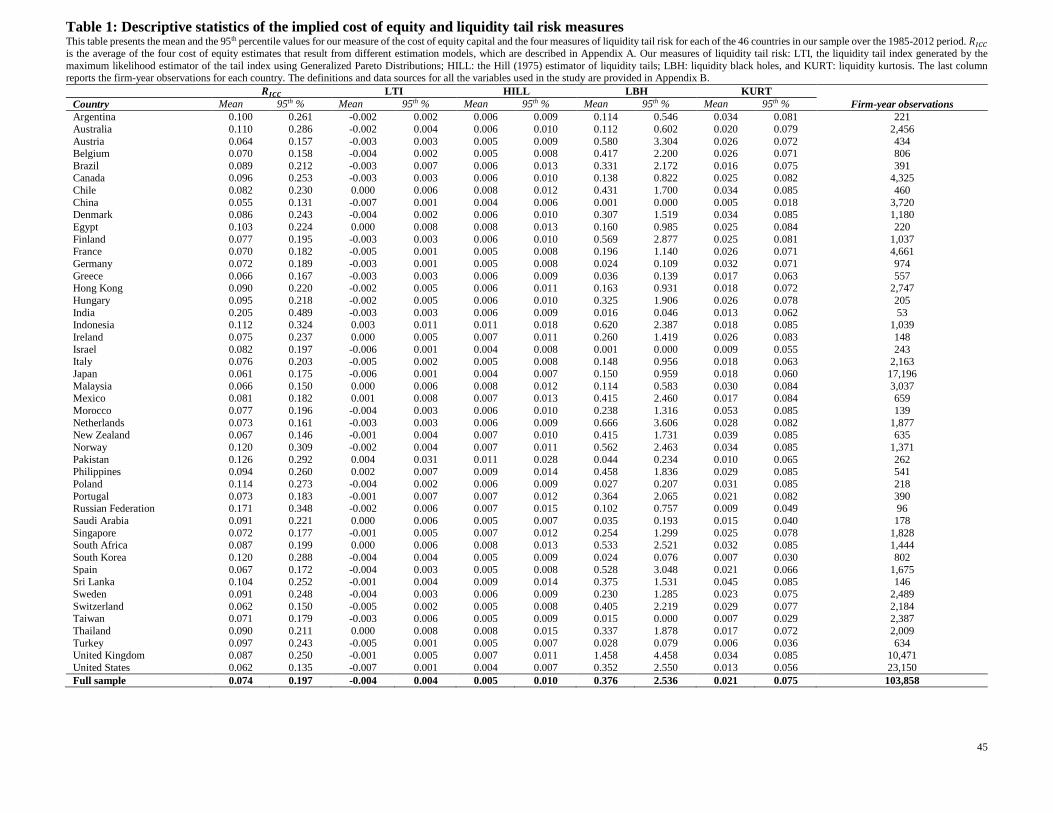
45

Table 1: Descriptive statistics of the implied cost of equity and liquidity tail risk measures This table presents the mean and the 95th percentile values for our measure of the cost of equity capital and the four measures of liquidity tail risk for each of the 46 countries in our sample over the 1985-2012 period. 𝑅𝐼𝐶𝐶 is the average of the four cost of equity estimates that result from different estimation models, which are described in Appendix A. Our measures of liquidity tail risk: LTI, the liquidity tail index generated by the

maximum likelihood estimator of the tail index using Generalized Pareto Distributions; HILL: the Hill (1975) estimator of liquidity tails; LBH: liquidity black holes, and KURT: liquidity kurtosis. The last column reports the firm-year observations for each country. The definitions and data sources for all the variables used in the study are provided in Appendix B.

𝑹𝑰𝑪𝑪 LTI HILL LBH KURT

Firm-year observations Country Mean 95th % Mean 95th % Mean 95th % Mean 95th % Mean 95th %

Argentina 0.100 0.261 -0.002 0.002 0.006 0.009 0.114 0.546 0.034 0.081 221

Australia 0.110 0.286 -0.002 0.004 0.006 0.010 0.112 0.602 0.020 0.079 2,456

Austria 0.064 0.157 -0.003 0.003 0.005 0.009 0.580 3.304 0.026 0.072 434 Belgium 0.070 0.158 -0.004 0.002 0.005 0.008 0.417 2.200 0.026 0.071 806

Brazil 0.089 0.212 -0.003 0.007 0.006 0.013 0.331 2.172 0.016 0.075 391 Canada 0.096 0.253 -0.003 0.003 0.006 0.010 0.138 0.822 0.025 0.082 4,325

Chile 0.082 0.230 0.000 0.006 0.008 0.012 0.431 1.700 0.034 0.085 460

China 0.055 0.131 -0.007 0.001 0.004 0.006 0.001 0.000 0.005 0.018 3,720 Denmark 0.086 0.243 -0.004 0.002 0.006 0.010 0.307 1.519 0.034 0.085 1,180

Egypt 0.103 0.224 0.000 0.008 0.008 0.013 0.160 0.985 0.025 0.084 220

Finland 0.077 0.195 -0.003 0.003 0.006 0.010 0.569 2.877 0.025 0.081 1,037 France 0.070 0.182 -0.005 0.001 0.005 0.008 0.196 1.140 0.026 0.071 4,661

Germany 0.072 0.189 -0.003 0.001 0.005 0.008 0.024 0.109 0.032 0.071 974

Greece 0.066 0.167 -0.003 0.003 0.006 0.009 0.036 0.139 0.017 0.063 557 Hong Kong 0.090 0.220 -0.002 0.005 0.006 0.011 0.163 0.931 0.018 0.072 2,747

Hungary 0.095 0.218 -0.002 0.005 0.006 0.010 0.325 1.906 0.026 0.078 205

India 0.205 0.489 -0.003 0.003 0.006 0.009 0.016 0.046 0.013 0.062 53 Indonesia 0.112 0.324 0.003 0.011 0.011 0.018 0.620 2.387 0.018 0.085 1,039

Ireland 0.075 0.237 0.000 0.005 0.007 0.011 0.260 1.419 0.026 0.083 148

Israel 0.082 0.197 -0.006 0.001 0.004 0.008 0.001 0.000 0.009 0.055 243 Italy 0.076 0.203 -0.005 0.002 0.005 0.008 0.148 0.956 0.018 0.063 2,163

Japan 0.061 0.175 -0.006 0.001 0.004 0.007 0.150 0.959 0.018 0.060 17,196

Malaysia 0.066 0.150 0.000 0.006 0.008 0.012 0.114 0.583 0.030 0.084 3,037 Mexico 0.081 0.182 0.001 0.008 0.007 0.013 0.415 2.460 0.017 0.084 659

Morocco 0.077 0.196 -0.004 0.003 0.006 0.010 0.238 1.316 0.053 0.085 139

Netherlands 0.073 0.161 -0.003 0.003 0.006 0.009 0.666 3.606 0.028 0.082 1,877

New Zealand 0.067 0.146 -0.001 0.004 0.007 0.010 0.415 1.731 0.039 0.085 635

Norway 0.120 0.309 -0.002 0.004 0.007 0.011 0.562 2.463 0.034 0.085 1,371

Pakistan 0.126 0.292 0.004 0.031 0.011 0.028 0.044 0.234 0.010 0.065 262 Philippines 0.094 0.260 0.002 0.007 0.009 0.014 0.458 1.836 0.029 0.085 541

Poland 0.114 0.273 -0.004 0.002 0.006 0.009 0.027 0.207 0.031 0.085 218

Portugal 0.073 0.183 -0.001 0.007 0.007 0.012 0.364 2.065 0.021 0.082 390 Russian Federation 0.171 0.348 -0.002 0.006 0.007 0.015 0.102 0.757 0.009 0.049 96

Saudi Arabia 0.091 0.221 0.000 0.006 0.005 0.007 0.035 0.193 0.015 0.040 178

Singapore 0.072 0.177 -0.001 0.005 0.007 0.012 0.254 1.299 0.025 0.078 1,828 South Africa 0.087 0.199 0.000 0.006 0.008 0.013 0.533 2.521 0.032 0.085 1,444

South Korea 0.120 0.288 -0.004 0.004 0.005 0.009 0.024 0.076 0.007 0.030 802

Spain 0.067 0.172 -0.004 0.003 0.005 0.008 0.528 3.048 0.021 0.066 1,675 Sri Lanka 0.104 0.252 -0.001 0.004 0.009 0.014 0.375 1.531 0.045 0.085 146

Sweden 0.091 0.248 -0.004 0.003 0.006 0.009 0.230 1.285 0.023 0.075 2,489

Switzerland 0.062 0.150 -0.005 0.002 0.005 0.008 0.405 2.219 0.029 0.077 2,184

Taiwan 0.071 0.179 -0.003 0.006 0.005 0.009 0.015 0.000 0.007 0.029 2,387

Thailand 0.090 0.211 0.000 0.008 0.008 0.015 0.337 1.878 0.017 0.072 2,009

Turkey 0.097 0.243 -0.005 0.001 0.005 0.007 0.028 0.079 0.006 0.036 634 United Kingdom 0.087 0.250 -0.001 0.005 0.007 0.011 1.458 4.458 0.034 0.085 10,471

United States 0.062 0.135 -0.007 0.001 0.004 0.007 0.352 2.550 0.013 0.056 23,150

Full sample 0.074 0.197 -0.004 0.004 0.005 0.010 0.376 2.536 0.021 0.075 103,858

46

Table 2: Descriptive statistics and correlation matrix This table reports descriptive statistics and Pearson's correlation coefficients for all variables used in our analyses. Panel A reports the descriptive statistics for the cost of capital as well as the explanatory variables used in the main analysis. The labels N, Mean, P25, P50, P75, and Std_dev reported in the first row in panel A stand for the number of observations, average, 25th percentile, median, 75th percentile, and the standard deviation,

respectively. Panel B reports Pearson's correlation coefficients among the liquidity tail risk variables (LTI, HILL, LBH, and KURT), liquidity level (Illiq), liquidity co-variances (𝐶𝑂𝑉(𝐼𝑙𝑙𝑖𝑞𝑖 , 𝐼𝑙𝑙𝑖𝑞𝑀), 𝐶𝑂𝑉(𝑟𝑖 , 𝐼𝑙𝑙𝑖𝑞𝑀),

𝐶𝑂𝑉(𝐼𝑙𝑙𝑖𝑞𝑖 , 𝑟𝑀), and 𝐶𝑂𝑉𝑛𝑒𝑡) and the cost of equity (𝑅𝐼𝐶𝐶). Panel C reports Pearson's correlation coefficients for the main control variables and the cost of equity. The total sample consists of 103,858 firm–year observations from 46 countries between 1985 and 2012. The definitions and data sources for all the variables used in the study are provided in Appendix B.

Panel A: Descriptive Statistics of the cost of equity and the explanatory variables stats N Mean P25 P50 P75 Std_dev

𝑅𝐼𝐶𝐶 103,858 0.0742 0.0406 0.0537 0.0805 0.0646

LTI 103,858 -0.0041 -0.0078 -0.0041 -0.0006 0.0050

HILL 103,858 0.0053 0.0033 0.0046 0.0066 0.0026 LBH 103,858 0.3755 0.0000 0.0000 0.1361 0.9585

LBH10 103,858 1.1194 0.0000 0.0397 1.5248 1.8839

LBH20 103,858 0.7206 0.0000 0.0000 0.6169 1.4480 LBH30 103,858 0.5450 0.0000 0.0000 0.3288 1.2158

LBH40 103,858 0.4429 0.0000 0.0000 0.2044 1.0656

KURT 103,858 0.0206 0.0018 0.0125 0.0356 0.0255 Illiq 103,858 0.0001 0.0000 0.0000 0.0000 0.0005

𝐶𝑂𝑉(𝐼𝑙𝑙𝑖𝑞𝑖 , 𝐼𝑙𝑙𝑖𝑞𝑀) 103,858 0.0001 0.0000 0.0000 0.0000 0.0006

𝐶𝑂𝑉(𝑟𝑖 , 𝐼𝑙𝑙𝑖𝑞𝑀) 103,858 -0.0004 -0.0003 -0.0000 -0.0000 0.0012

𝐶𝑂𝑉(𝐼𝑙𝑙𝑖𝑞𝑖 , 𝑟𝑀) 103,858 -0.0001 -0.0000 -0.0000 -0.0000 0.0004

BETA 103,858 0.9826 0.6031 0.9367 1.2894 0.5706 BTM 103,858 1.0249 0.2981 0.5397 0.8550 8.7845

LEVERAGE 103,858 0.3109 0.0502 0.2499 0.5076 0.2800

SIZE 103,858 13.8006 12.4584 13.6494 14.9797 1.9175 LNGDP 101,409 10.0914 10.2351 10.4311 10.5273 0.9036

FD 99,609 103.8988 63.3462 90.0500 130.6177 69.0962

INF 95,297 2.4403 1.1580 2.1349 3.2541 3.4000

Panel B: Pearson’s correlations between liquidity tail risk measures, liquidity level, liquidity covariance risks, and the implied cost of capital 𝑹𝑰𝑪𝑪 LTI HILL LBH KURT Illiq 𝑪𝑶𝑽(𝑰𝒍𝒍𝒊𝒒𝒊, 𝑰𝒍𝒍𝒊𝒒𝑴) 𝑪𝑶𝑽(𝒓𝒊, 𝑰𝒍𝒍𝒊𝒒𝑴) 𝑪𝑶𝑽(𝑰𝒍𝒍𝒊𝒒𝒊, 𝒓𝑴) 𝐂𝐎𝐕𝐧𝐞𝐭

𝑅𝐼𝐶𝐶 1.000

LTI 0.178 1.000

HILL 0.210 0.762 1.000 LBH 0.184 0.189 0.282 1.000

KURT 0.081 0.334 0.412 0.359 1.000

Illiq 0.115 0.139 0.172 0.029 -0.100 1.000

𝐶𝑂𝑉(𝐼𝑙𝑙𝑖𝑞𝑖 , 𝐼𝑙𝑙𝑖𝑞𝑀) 0.116 0.125 0.151 0.028 0.033 0.641 1.000

𝐶𝑂𝑉(𝑟𝑖 , 𝐼𝑙𝑙𝑖𝑞𝑀) -0.087 -0.097 -0.098 0.072 -0.021 -0.196 -0.319 1.000

𝐶𝑂𝑉(𝐼𝑙𝑙𝑖𝑞𝑖 , 𝑟𝑀) -0.116 -0.163 -0.209 -0.075 -0.014 -0.678 -0.591 0.248 1.000

COVnet 0.127 0.148 0.167 -0.026 0.029 0.505 0.697 -0.882 -0.596 1.000

Panel C: Pearson’s correlations between main control variables and the implied cost of capital RICC BETA BTM LEVERAGE SIZE LNGDP FD INF

RICC 1.000

BETA 0.097 1.000

BTM 0.098 0.005 1.000

LEVERAGE 0.083 0.039 0.116 1.000

SIZE -0.202 0.142 0.015 0.340 1.000 LNGDP -0.045 0.063 -0.082 -0.060 0.133 1.000

FD 0.003 -0.021 -0.010 -0.177 -0.031 0.117 1.000

INF 0.095 -0.021 0.057 0.069 -0.037 -0.363 -0.117 1.000

47

Table 3: Liquidity tail index (LTI) and the implied cost of equity This table reports pooled OLS regression results of the following implied cost of equity capital model:

𝑅𝐼𝐶𝐶𝑡

𝑖 = 𝛼0 + 𝛽1𝐿𝑇𝐼𝑡𝑖 + 𝛽2𝐶𝑜𝑛𝑡𝑟𝑜𝑙𝑠𝑡 + 𝐹𝐸 + 𝜀𝑡

𝑖

For firm i in year t, the dependent variable 𝑅𝐼𝐶𝐶𝑡

𝑖 is the average of the four implied cost of equity capital models described in Appendix A. Liquidity tail risk, LTI, is defined as the liquidity tail index generated by the

maximum likelihood estimator of the tail index using Generalized Pareto Distributions. The set of control variables (𝐶𝑜𝑛𝑡𝑟𝑜𝑙𝑠) is comprised of: Illiq: defined as the innovation in stock liquidity using Amihud (2002)

model, 𝐶𝑂𝑉(𝐼𝑙𝑙𝑖𝑞𝑖 , 𝐼𝑙𝑙𝑖𝑞𝑀): co-movement between firm-level liquidity and market liquidity, 𝐶𝑂𝑉(𝑟𝑖 , 𝐼𝑙𝑙𝑖𝑞𝑀): co-movement between firm-level returns and market liquidity, 𝐶𝑂𝑉(𝐼𝑙𝑙𝑖𝑞𝑖 , 𝑟𝑀): co-movement between

firm-level liquidity and market returns, and 𝐶𝑂𝑉𝑛𝑒𝑡𝑖 = 𝐶𝑂𝑉(𝐼𝑙𝑙𝑖𝑞𝑖 , 𝐼𝑙𝑙𝑖𝑞𝑀) − 𝐶𝑂𝑉(𝑟𝑖 , 𝐼𝑙𝑙𝑖𝑞𝑀) − 𝐶𝑂𝑉(𝐼𝑙𝑙𝑖𝑞𝑖 , 𝑟𝑀), and other determinants at the firm-level and the country-level. FE is the set of fixed effects at the

country, industry, and year levels. The firm-level variables are: SIZE, estimated as the natural logarithm of a firm’s total assets; BETA, estimated as the co-variance between the firm returns and the market return relative

to the variance of the market returns; LEVERAGE, computed as total debt to the market value of equity; and BTM, computed as the book value of equity divided by the market value of equity. The country-level variables

are: LNGDP, Logarithm of GDP per capita; INFL, measured as the annualized yearly median of a country-specific one-year-ahead realized monthly inflation rate; and FD, calculated as the sum of market capitalization and private credit relative to GDP. The total sample consists of 103,858 firm–year observations from 46 countries between 1985 and 2012. The definitions and data sources for all the variables used in the study are

provided in Appendix B. Beneath each coefficient is the robust t-statistic clustered at the country level.

(1) (2) (3) (4) (5) (6) (7) (8) (9) (10)

Variables 𝑹𝑰𝑪𝑪 𝑹𝑰𝑪𝑪 𝑹𝑰𝑪𝑪 𝑹𝑰𝑪𝑪 𝑹𝑰𝑪𝑪 𝑹𝑰𝑪𝑪 𝑹𝑰𝑪𝑪 𝑹𝑰𝑪𝑪 𝑹𝑰𝑪𝑪 𝑹𝑰𝑪𝑪

LTI 0.701*** 0.701*** 0.699*** 0.699*** 0.697*** 0.621*** 0.621*** 0.618*** 0.618*** 0.616***

(6.178) (6.310) (6.235) (6.175) (6.299) (5.724) (5.789) (5.773) (5.714) (5.807)

Illiq 7.220*** 3.868* 7.195*** 5.340** 5.180*** 6.403*** 3.254** 6.363*** 4.114** 4.336***

(3.281) (1.966) (3.297) (2.294) (2.794) (3.786) (2.267) (3.812) (2.608) (3.095)

𝐶𝑂𝑉(𝐼𝑙𝑙𝑖𝑞𝑖 , 𝐼𝑙𝑙𝑖𝑞𝑀) 4.849** 4.496*

(2.142) (1.996)

𝐶𝑂𝑉(𝑟𝑖 , 𝐼𝑙𝑙𝑖𝑞𝑀) -1.305** -1.264*

(-2.553) (-1.941)

𝐶𝑂𝑉(𝐼𝑙𝑙𝑖𝑞𝑖 , 𝑟𝑀) -3.940* -4.587**

(-1.991) (-2.417)

COVnet 1.718*** 1.679**

(2.885) (2.314)

BETA 0.016*** 0.016*** 0.016*** 0.016*** 0.016*** 0.016*** 0.016*** 0.015*** 0.016*** 0.015*** (7.993) (8.098) (8.146) (8.032) (8.172) (8.614) (8.729) (8.822) (8.649) (8.858)

BTM 0.000*** 0.000*** 0.000*** 0.000*** 0.000*** 0.000*** 0.000*** 0.000*** 0.000*** 0.000***

(4.312) (4.311) (4.317) (4.312) (4.318) (5.166) (5.165) (5.168) (5.168) (5.169) LEVERAGE 0.049*** 0.049*** 0.049*** 0.049*** 0.049*** 0.049*** 0.049*** 0.049*** 0.049*** 0.049***

(12.400) (12.137) (12.350) (12.265) (12.179) (12.493) (12.213) (12.444) (12.310) (12.254)

SIZE -0.009*** -0.008*** -0.008*** -0.008*** -0.008*** -0.009*** -0.008*** -0.009*** -0.008*** -0.008*** (-5.245) (-5.106) (-5.226) (-5.148) (-5.129) (-5.298) (-5.161) (-5.279) (-5.191) (-5.178)

LNGDP -0.013 -0.013 -0.013 -0.013 -0.013

(-0.627) (-0.603) (-0.624) (-0.606) (-0.605) FD -0.000 -0.000 -0.000 -0.000 -0.000*

(-1.512) (-1.601) (-1.666) (-1.652) (-1.795)

INF 0.001*** 0.001*** 0.001*** 0.001*** 0.001*** (9.481) (9.523) (8.855) (9.411) (8.649)

Constant 0.156*** 0.154*** 0.155*** 0.154*** 0.153*** 0.263 0.259 0.262 0.257 0.257 (10.007) (9.711) (9.836) (9.697) (9.512) (1.500) (1.465) (1.499) (1.464) (1.474)

Observations 103,858 103,858 103,858 103,858 103,858 93,433 93,433 93,433 93,433 93,433

Adjusted R-squared 0.179 0.180 0.180 0.179 0.180 0.178 0.179 0.179 0.179 0.179

48

Table 4: Liquidity tail risk (HILL and KURT) and the implied cost of equity This table reports pooled OLS regression results of the following implied cost of equity capital model:

𝑅𝐼𝐶𝐶𝑡

𝑖 = 𝛼0 + 𝛽1𝐿𝑇𝑅𝑡𝑖 + 𝛽2𝐶𝑜𝑛𝑡𝑟𝑜𝑙𝑠𝑡 + 𝐹𝐸 + 𝜀𝑡

𝑖

For firm i in year t, the dependent variable 𝑅𝐼𝐶𝐶𝑡

𝑖 is the average of the four implied cost of equity capital estimates described in Appendix A. 𝐿𝑇𝑅 stands for liquidity tail risk and is either HILL or KURT, which are

respectively defined as the Hill (1975) estimator of liquidity tails, and the kurtosis in the liquidity distribution. The set of control variables (𝐶𝑜𝑛𝑡𝑟𝑜𝑙𝑠) is comprised of: Illiq, defined as the innovation in stock liquidity

using Amihud (2002) model; 𝐶𝑂𝑉(𝐼𝑙𝑙𝑖𝑞𝑖 , 𝐼𝑙𝑙𝑖𝑞𝑀): co-movement between firm-level liquidity and market liquidity; 𝐶𝑂𝑉(𝑟𝑖 , 𝐼𝑙𝑙𝑖𝑞𝑀): co-movement between firm-level returns and market liquidity; 𝐶𝑂𝑉(𝐼𝑙𝑙𝑖𝑞𝑖 , 𝑟𝑀): co-

movement between firm-level liquidity and market returns; and 𝐶𝑂𝑉𝑛𝑒𝑡𝑖 = 𝐶𝑂𝑉(𝐼𝑙𝑙𝑖𝑞𝑖 , 𝐼𝑙𝑙𝑖𝑞𝑀) − 𝐶𝑂𝑉(𝑟𝑖 , 𝐼𝑙𝑙𝑖𝑞𝑀) − 𝐶𝑂𝑉(𝐼𝑙𝑙𝑖𝑞𝑖 , 𝑟𝑀); and other determinants at the firm-level and the country-level. FE is the set of

fixed effects at the country, industry, and year levels. The firm-level variables are: SIZE, estimated as the natural logarithm of the firm’s total assets; BETA, estimated as the co-variance between the firm returns and the

market return relative to the variance of the market returns; LEVERAGE, computed as total debt to the market value of equity; and BTM, computed as book value of equity divided by the market value of equity. The

country-level variables are: LNGDP: Logarithm of GDP per capita; INFL: measured as the annualized yearly median of a country-specific one-year-ahead realized monthly inflation rate; and FD: calculated as the sum of market capitalization and private credit relative to GDP. The definitions and data sources for all the variables used in the study are provided in Appendix B. Beneath each coefficient is the robust t-statistic clustered

at the country level.

(1) (2) (3) (4) (5) (6) (7) (8) (9) (10)

Variables 𝑹𝑰𝑪𝑪 𝑹𝑰𝑪𝑪 𝑹𝑰𝑪𝑪 𝑹𝑰𝑪𝑪 𝑹𝑰𝑪𝑪 𝑹𝑰𝑪𝑪 𝑹𝑰𝑪𝑪 𝑹𝑰𝑪𝑪 𝑹𝑰𝑪𝑪 𝑹𝑰𝑪𝑪

HILL 1.943*** 1.925*** 1.936*** 1.921*** 1.918***

(6.434) (6.452) (6.467) (6.347) (6.463)

KURT 0.108** 0.100** 0.109** 0.106** 0.105**

(2.473) (2.411) (2.488) (2.442) (2.454)

Illiq 5.998*** 2.987** 5.960*** 3.954** 4.013*** 7.732*** 4.841*** 7.693*** 5.511*** 5.686***

(3.603) (2.095) (3.622) (2.553) (2.877) (4.000) (2.958) (4.028) (3.082) (3.526)

𝐶𝑂𝑉(𝐼𝑙𝑙𝑖𝑞𝑖 , 𝐼𝑙𝑙𝑖𝑞𝑀) 4.306* 4.013*

(1.968) (1.843)

𝐶𝑂𝑉(𝑟𝑖 , 𝐼𝑙𝑙𝑖𝑞𝑀) -1.242* -1.289*

(-1.931) (-2.006)

𝐶𝑂𝑉(𝐼𝑙𝑙𝑖𝑞𝑖 , 𝑟𝑀) -4.108** -4.413**

(-2.201) (-2.421)

COVnet 1.618** 1.631**

(2.275) (2.303)

BETA 0.016*** 0.016*** 0.016*** 0.016*** 0.016*** 0.017*** 0.016*** 0.016*** 0.017*** 0.016*** (8.914) (9.030) (9.125) (8.945) (9.159) (9.581) (9.792) (9.966) (9.588) (10.086)

BTM 0.000*** 0.000*** 0.000*** 0.000*** 0.000*** 0.000*** 0.000*** 0.000*** 0.000*** 0.000***

(5.235) (5.234) (5.237) (5.237) (5.238) (5.205) (5.206) (5.207) (5.207) (5.209) LEVERAGE 0.048*** 0.048*** 0.048*** 0.048*** 0.048*** 0.049*** 0.049*** 0.049*** 0.049*** 0.049***

(12.487) (12.250) (12.445) (12.336) (12.281) (11.501) (11.390) (11.461) (11.360) (11.348)

SIZE -0.008*** -0.008*** -0.008*** -0.008*** -0.008*** -0.009*** -0.009*** -0.009*** -0.008*** -0.008*** (-5.048) (-4.941) (-5.031) (-4.966) (-4.949) (-4.733) (-4.684) (-4.715) (-4.652) (-4.656)

LNGDP -0.015 -0.015 -0.015 -0.015 -0.015 -0.013 -0.013 -0.013 -0.013 -0.012

(-0.723) (-0.696) (-0.719) (-0.701) (-0.700) (-0.618) (-0.590) (-0.614) (-0.596) (-0.594) FD -0.000 -0.000 -0.000 -0.000 -0.000* -0.000 -0.000 -0.000 -0.000 -0.000*

(-1.513) (-1.608) (-1.672) (-1.647) (-1.803) (-1.460) (-1.566) (-1.626) (-1.612) (-1.765)

INF 0.001*** 0.001*** 0.001*** 0.001*** 0.001*** 0.001*** 0.001*** 0.001*** 0.001*** 0.001*** (9.604) (9.597) (9.035) (9.553) (8.849) (9.709) (9.688) (9.101) (9.640) (8.915)

Constant 0.256 0.251 0.254 0.250 0.250 0.252 0.248 0.251 0.246 0.246

(1.496) (1.462) (1.496) (1.463) (1.470) (1.464) (1.430) (1.463) (1.429) (1.437)

Observations 93,433 93,433 93,433 93,433 93,433 93,433 93,433 93,433 93,433 93,433 Adjusted R-squared 0.180 0.181 0.181 0.181 0.181 0.178 0.179 0.178 0.178 0.179

49

Table 5: Liquidity black holes and the implied cost of equity This table reports pooled OLS regression results of the following implied cost of equity capital model:

𝑅𝐼𝐶𝐶𝑡

𝑖 = 𝛼0 + 𝛽1𝐿𝐵𝐻𝑡𝑖 + 𝛽2𝐶𝑜𝑛𝑡𝑟𝑜𝑙𝑠𝑡 + 𝐹𝐸 + 𝜀𝑡

𝑖

For firm i in year t, the dependent variable 𝑅𝐼𝐶𝐶𝑡

𝑖 is the average of the four implied cost of equity capital estimates described in Appendix A. LBH stands for liquidity black holes which measure the frequency of extreme

liquidity events defined when the firm illiquidity level exceeds a predefined multiple (50 times) of the market average liquidity. In the table below, LBH10, LBH20, LBH30, and LBH40 respectively record an extreme

liquidity event when the firm illiquidity is more than 10, 20, 30, and 40 times the market average illiquidity. The set of control variables (𝐶𝑜𝑛𝑡𝑟𝑜𝑙𝑠) is comprised of: Illiq, defined as the innovation in stock liquidity

using Amihud (2002) model; 𝐶𝑂𝑉(𝐼𝑙𝑙𝑖𝑞𝑖 , 𝐼𝑙𝑙𝑖𝑞𝑀): co-movement between firm-level liquidity and market liquidity; 𝐶𝑂𝑉(𝑟𝑖 , 𝐼𝑙𝑙𝑖𝑞𝑀): co-movement between firm-level returns and market liquidity; 𝐶𝑂𝑉(𝐼𝑙𝑙𝑖𝑞𝑖 , 𝑟𝑀): co-

movement between firm-level liquidity and market returns; and 𝐶𝑂𝑉𝑛𝑒𝑡𝑖 = 𝐶𝑂𝑉(𝐼𝑙𝑙𝑖𝑞𝑖 , 𝐼𝑙𝑙𝑖𝑞𝑀) − 𝐶𝑂𝑉(𝑟𝑖 , 𝐼𝑙𝑙𝑖𝑞𝑀) − 𝐶𝑂𝑉(𝐼𝑙𝑙𝑖𝑞𝑖 , 𝑟𝑀); and other determinants at the firm-level and the country-level. FE is the set of

fixed effects dummy variables at the country, industry, and year levels. The firm-level variables are: SIZE: estimated as the natural logarithm of the firm’s total assets; BETA: estimated as the co-variance between the

firm returns and the market return relative to the variance of the market returns; LEVERAGE: computed as total debt to the market value of equity; and BTM: computed as book value of equity divided by the market value of equity. The country-level variables are: LNGDP: Logarithm of GDP per capita; INFL: measured as the annualized yearly median of a country-specific one-year-ahead realized monthly inflation rate; and FD:

calculated as the sum of market capitalization and private credit relative to GDP. The definitions and data sources for all the variables used in the study are provided in Appendix B. Beneath each coefficient is the robust

t-statistic clustered at the country level.

(1) (2) (3) (4) (5) (6) (7) (8) (9) VARIABLES 𝑹𝑰𝑪𝑪 𝑹𝑰𝑪𝑪 𝑹𝑰𝑪𝑪 𝑹𝑰𝑪𝑪 𝑹𝑰𝑪𝑪 𝑹𝑰𝑪𝑪 𝑹𝑰𝑪𝑪 𝑹𝑰𝑪𝑪 𝑹𝑰𝑪𝑪

LBH 0.008*** 0.008*** 0.008*** 0.008*** 0.008***

(4.537) (4.455) (4.536) (4.449) (4.465)

LBH10 0.004***

(4.139)

LBH20 0.005***

(4.212)

LBH30 0.006***

(4.279)

LBH40 0.007***

(4.350)

Illiq 6.740*** 3.865*** 6.697*** 5.154*** 4.742*** 4.269*** 4.473*** 4.603*** 4.690***

(4.223) (2.705) (4.266) (3.410) (3.588) (3.042) (3.268) (3.420) (3.523)

𝐶𝑂𝑉(𝐼𝑙𝑙𝑖𝑞𝑖 , 𝐼𝑙𝑙𝑖𝑞𝑀) 4.104*

(1.850)

𝐶𝑂𝑉(𝑟𝑖 , 𝐼𝑙𝑙𝑖𝑞𝑀) -1.341**

(-2.084)

𝐶𝑂𝑉(𝐼𝑙𝑙𝑖𝑞𝑖 , 𝑟𝑀) -3.177*

(-1.826)

COVnet 1.621** 1.594** 1.598** 1.605** 1.613**

(2.258) (2.179) (2.200) (2.220) (2.239)

BETA 0.017*** 0.017*** 0.016*** 0.017*** 0.016*** 0.017*** 0.017*** 0.017*** 0.017***

(9.340) (9.449) (9.584) (9.362) (9.585) (8.688) (9.107) (9.321) (9.463) BTM 0.000*** 0.000*** 0.000*** 0.000*** 0.000*** 0.000*** 0.000*** 0.000*** 0.000***

(5.411) (5.410) (5.414) (5.411) (5.414) (5.376) (5.408) (5.405) (5.403)

LEVERAGE 0.045*** 0.045*** 0.045*** 0.045*** 0.045*** 0.044*** 0.044*** 0.044*** 0.045*** (15.718) (15.408) (15.622) (15.646) (15.437) (12.725) (14.216) (14.822) (15.200)

SIZE -0.007*** -0.007*** -0.007*** -0.007*** -0.007*** -0.007*** -0.007*** -0.007*** -0.007***

(-6.478) (-6.354) (-6.492) (-6.442) (-6.419) (-5.019) (-5.746) (-6.085) (-6.299) LNGDP -0.014 -0.014 -0.014 -0.014 -0.014 -0.015 -0.015 -0.014 -0.014

(-0.693) (-0.668) (-0.689) (-0.676) (-0.671) (-0.751) (-0.733) (-0.709) (-0.687)

FD -0.000 -0.000 -0.000 -0.000 -0.000* -0.000* -0.000* -0.000* -0.000*

(-1.518) (-1.582) (-1.659) (-1.612) (-1.751) (-1.742) (-1.741) (-1.745) (-1.749)

INF 0.001*** 0.001*** 0.001*** 0.001*** 0.001*** 0.001*** 0.001*** 0.001*** 0.001***

(8.342) (8.277) (8.091) (8.357) (8.005) (8.321) (8.253) (8.155) (8.073) Constant 0.252 0.248 0.251 0.248 0.246 0.247 0.249 0.248 0.247

(1.480) (1.447) (1.479) (1.454) (1.454) (1.513) (1.507) (1.487) (1.468)

Observations 93,433 93,433 93,433 93,433 93,433 93,433 93,433 93,433 93,433

Adjusted R-squared 0.187 0.188 0.188 0.187 0.188 0.186 0.187 0.188 0.188

50

Table 6: Liquidity tail index and the implied cost of equity during crisis periods This table reports pooled OLS regression results of the following implied cost of equity capital model:

𝑅𝐼𝐶𝐶𝑡

𝑖 = 𝛼0 + 𝛽1𝐿𝑇𝐼𝑡𝑖 + 𝛽2𝑀𝑘𝑡𝐶𝑜𝑛𝑑𝑖𝑡𝑖𝑜𝑛𝑡 + 𝛽3𝐿𝑇𝐼 × 𝑀𝑘𝑡𝐶𝑜𝑛𝑑𝑖𝑡𝑖𝑜𝑛𝑡

𝑖 + 𝛽4𝐶𝑜𝑛𝑡𝑟𝑜𝑙𝑠𝑡 + 𝐹𝐸 + 𝜀𝑡𝑖

For firm i in year t, the dependent variable 𝑅𝐼𝐶𝐶𝑡

𝑖 is the average of the four implied cost of equity capital estimates described in Appendix A. LTI is defined as the liquidity tail index generated by the maximum likelihood

estimator of the tail index using Generalized Pareto Distributions. 𝑀𝑘𝑡𝐶𝑜𝑛𝑑𝑖𝑡𝑖𝑜𝑛 is either 𝑀𝑘𝑡𝐷𝑜𝑤𝑛 or 𝑀𝑘𝑡𝑉𝑜𝑙. The dummy variable 𝑀𝑘𝑡𝐷𝑜𝑤𝑛 (𝑀𝑘𝑡𝑉𝑜𝑙) takes on one when the country’s stock market returns

(volatility) drops below (exceeds) its 3-year historical moving average by more than one standard deviation; and zero otherwise. The set of control variables (𝐶𝑜𝑛𝑡𝑟𝑜𝑙𝑠) is comprised of: Illiq: defined as the innovation

in stock liquidity using Amihud (2002) model; 𝐶𝑂𝑉𝑛𝑒𝑡𝑖 = 𝐶𝑂𝑉(𝐼𝑙𝑙𝑖𝑞𝑖 , 𝐼𝑙𝑙𝑖𝑞𝑀) − 𝐶𝑂𝑉(𝑟𝑖 , 𝐼𝑙𝑙𝑖𝑞𝑀) − 𝐶𝑂𝑉(𝐼𝑙𝑙𝑖𝑞𝑖 , 𝑟𝑀); and other determinants at the firm-level and the country-level. FE is the set of fixed effects dummy

variables at the country, industry, and year levels. The firm-level variables are: SIZE: estimated as the natural logarithm of the firm’s total assets; BETA: estimated as the co-variance between the firm returns and the

market return relative to the variance of the market returns; LEVERAGE: computed as total debt to the market value of equity; and BTM: computed as book value of equity divided by the market value of equity. The country-level variables are: LNGDP: Logarithm of GDP per capita; INFL: measured as the annualized yearly median of a country-specific one-year-ahead realized monthly inflation rate; and FD: calculated as the sum

of market capitalization and private credit relative to GDP. The definitions and data sources for all the variables used in the study are provided in Appendix B. Beneath each coefficient is the robust t-statistic clustered

at the country level.

(1) (2) (3) (4)

Variables 𝑹𝑰𝑪𝑪 𝑹𝑰𝑪𝑪 𝑹𝑰𝑪𝑪 𝑹𝑰𝑪𝑪

LTI 0.678*** 0.594*** 0.662*** 0.576***

(6.238) (5.687) (5.797) (5.332)

Mktdown 0.003 0.003

(0.838) (0.876)

LTI*Mktdown 1.995** 2.045**

(2.216) (2.309)

MktVol 0.031*** 0.029***

(3.052) (2.769)

LTI*MktVol 2.814** 2.787**

(2.659) (2.487)

Illiq 5.201*** 4.359*** 5.261*** 4.426***

(2.816) (3.132) (2.839) (3.125) COVnet 1.715*** 1.676** 1.752*** 1.689**

(2.880) (2.307) (2.901) (2.309)

BETA 0.016*** 0.015*** 0.016*** 0.015***

(8.178) (8.862) (8.242) (8.921)

BTM 0.000*** 0.000*** 0.001*** 0.000***

(4.318) (5.172) (4.423) (5.329)

LEVERAGE 0.049*** 0.049*** 0.049*** 0.048***

(12.317) (12.383) (12.188) (12.252)

SIZE -0.008*** -0.008*** -0.008*** -0.008***

(-5.152) (-5.203) (-5.124) (-5.176)

LNGDP -0.013 -0.015

(-0.626) (-0.678)

FD -0.000* -0.000

(-1.803) (-1.133)

INF 0.001*** 0.001***

(8.618) (7.777)

Constant 0.153*** 0.260 0.154*** 0.272

(9.567) (1.498) (9.540) (1.546)

Observations 103,858 93,433 103,858 93,433

Adjusted R-squared 0.180 0.179 0.182 0.181

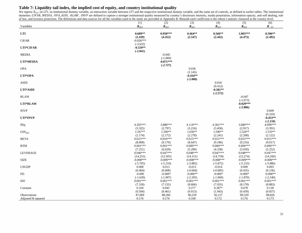
51

Table 7: Liquidity tail index, the implied cost of equity, and country institutional quality We regress 𝑅𝐼𝐶𝐶 on 𝐿𝑇𝐼, an institutional dummy variable, an interaction variable between 𝐿𝑇𝐼 and the respective institutional dummy variable, and the same set of controls, as defined in earlier tables. The institutional

dummies: 𝐶𝐼𝐹𝐴𝑅, 𝑀𝐸𝐷𝐼𝐴, 𝑂𝑃𝐴, 𝐴𝑆𝐷𝐼, 𝑅𝐿𝐴𝑊, 𝐼𝑁𝑉𝑃 are defined to capture a stronger institutional quality measured by country’s disclosure intensity, media penetration, information opacity, anti-self dealing, rule of law, and investor protection. The definitions and data sources for all the variables used in the study are provided in Appendix B. Beneath each coefficient is the robust t-statistic clustered at the country level.

(1) (2) (3) (4) (5) (6)

Variables 𝑹𝑰𝑪𝑪 𝑹𝑰𝑪𝑪 𝑹𝑰𝑪𝑪 𝑹𝑰𝑪𝑪 𝑹𝑰𝑪𝑪 𝑹𝑰𝑪𝑪

LTI 0.689** 0.950*** 0.464** 0.566** 1.003*** 0.506**

(2.439) (4.452) (2.547) (2.442) (4.473) (2.492)

CIFAR -0.026***

(-3.632)

LTI*CIFAR -0.559**

(-2.041)

MEDIA -0.045 (-1.069)

LTI*MEDIA -0.871***

(-2.727)

OPA 0.036

(1.145)

LTI*OPA -0.434**

(-2.080)

ASDI 0.018

(0.412)

LTI*ASDI -0.581**

(-2.572)

RLAW -0.047 (-1.073)

LTI*RLAW -0.929***

(-2.806)

INVP 0.009

(0.310)

LTI*INVP -0.453**

(-2.110)

Illiq 4.205*** 3.888*** 4.114*** 4.361*** 3.680*** 4.099***

(3.325) (2.797) (3.216) (3.458) (2.917) (3.391)

COVnet 1.567** 1.560** 1.656** 1.590** 1.524** 1.533**

(2.174) (2.172) (2.278) (2.241) (2.208) (2.122)

BETA 0.015*** 0.016*** 0.015*** 0.015*** 0.015*** 0.015***

(8.808) (9.170) (8.647) (9.186) (9.216) (9.017) BTM 0.001*** 0.001*** 0.000*** 0.000*** 0.000*** 0.000***

(7.251) (6.629) (5.290) (4.338) (5.030) (5.252)

LEVERAGE 0.046*** 0.047*** 0.048*** 0.047*** 0.048*** 0.047*** (14.253) (12.505) (14.151) (14.759) (12.274) (14.160)

SIZE -0.008*** -0.009*** -0.008*** -0.008*** -0.009*** -0.008***

(-5.705) (-5.210) (-5.882) (-5.872) (-5.233) (-5.886) LNGDP 0.008 0.013 -0.013 -0.014 0.009 0.003

(0.404) (0.608) (-0.684) (-0.685) (0.435) (0.136)

FD -0.000 -0.000* -0.000** -0.000* -0.000* -0.000**

(-1.639) (-1.907) (-2.205) (-1.969) (-1.870) (-2.240)

INF 0.001*** 0.001*** 0.001*** 0.001*** 0.001*** 0.001***

(7.318) (7.155) (8.606) (7.035) (8.178) (8.883) Constant 0.104 0.045 0.277 0.387* 0.078 0.130

(0.594) (0.461) (0.013) (1.943) (0.439) (0.837)

Observations 87,869 88,266 90,259 92,157 89,329 88,826 Adjusted R-squared 0.176 0.176 0.169 0.172 0.176 0.173

52

Table 8: Robustness checks In Panel A, we follow two-step regression model. In the first step, we separately orthogonalize each of 𝐿𝑇𝐼, 𝐻𝐼𝐿𝐿, 𝐿𝐵𝐻 , 𝐾𝑈𝑅𝑇 on 𝐶𝑂𝑉𝑛𝑒𝑡 and collect the resulting residuals: res_LTI, res_HILL, res_LBH, and

res_KURT, respectively. In the second step, we re-estimate four models by regressing 𝑅𝐼𝐶𝐶 on each of res_LTI, res_HILL, res_LBH, and res_KURT, and on the same set of control variables, excluding 𝐶𝑂𝑉𝑛𝑒𝑡.

In Panel B, columns (1)-(4) repeat the same analysis as in Table 3 model (10) after replacing 𝑅𝐼𝐶𝐶 with each of 𝑅ES, RGLS, 𝑅OJ, and 𝑅CT that represent the implied cost of equity estimates of Easton (2004), Gebhardt et

al. (2001), Ohlson and Juettner-Nauroth (2005), and Claus and Thomas (2001), respectively. All remaining columns use 𝑅𝐼𝐶𝐶 as the dependent variable. Columns (5) and (6) estimate the model after excluding U.S. firms and financial firms, respectively. Columns (7) –(11) separately introduce an additional control variable at a time: FBIAS, defined as the difference between the one-year-ahead forecasted and realized earnings;

LTG: the firm’s long-term earnings growth; Dispersion: measured as the ratio of the standard deviation of estimated first year earnings per share by the average forecasted first year earnings per share; ANALYSTCOV: measured as the number of analysts who are covering the firm by providing earnings forecasts; CROSSLIST: takes the value of one for firms that cross-list in the U.S. and zero otherwise.

The four cost of equity models are defined in Appendix A. The definitions and data sources for all the variables used in the study are provided in Appendix B. Beneath each coefficient is the robust t-statistic clustered

at the country level.

Panel A (1) (2) (3) (4)

VARIABLES 𝑹𝑰𝑪𝑪 𝑹𝑰𝑪𝑪 𝑹𝑰𝑪𝑪 𝑹𝑰𝑪𝑪

res_LTI 0.616***

(5.807)

res_HILL 1.918***

(6.463)

res_LBH 0.008***

(4.465)

res_KURT 0.105**

(2.454)

Illiq 4.336*** 4.013*** 4.742*** 5.686***

(3.095) (2.877) (3.588) (3.526) COVnet 1.818** 1.952*** 1.982*** 1.606**

(2.501) (2.694) (2.865) (2.280)

BETA 0.015*** 0.016*** 0.016*** 0.016***

(8.858) (9.159) (9.585) (10.086)

BTM 0.000*** 0.000*** 0.000*** 0.000***

(5.169) (5.238) (5.414) (5.209)

LEVERAGE 0.049*** 0.048*** 0.045*** 0.049***

(12.254) (12.281) (15.437) (11.348)

SIZE -0.008*** -0.008*** -0.007*** -0.008***

(-5.178) (-4.949) (-6.419) (-4.656)

LNGDP -0.013 -0.015 -0.014 -0.012

(-0.605) (-0.700) (-0.671) (-0.594)

FD -0.000* -0.000* -0.000* -0.000*

(-1.795) (-1.803) (-1.751) (-1.765)

INF 0.001*** 0.001*** 0.001*** 0.001***

(8.649) (8.849) (8.005) (8.915)

Constant 0.257 0.263 0.247 0.252

(1.471) (1.550) (1.460) (1.473)

Observations 93,433 93,433 93,433 93,433

Adjusted R-squared 0.179 0.181 0.188 0.179

53

Panel B (1) (2) (3) (4) (5) (6) (7) (8) (9) (10) (11)

Variables 𝑹𝑬𝑺 𝑹𝑮𝑳𝑺 𝑹𝑶𝑱 𝑹𝑪𝑻 𝑹𝑰𝑪𝑪 𝑹𝑰𝑪𝑪 𝑹𝑰𝑪𝑪 𝑹𝑰𝑪𝑪 𝑹𝑰𝑪𝑪 𝑹𝑰𝑪𝑪 𝑹𝑰𝑪𝑪

LTI 0.751*** 0.454*** 0.446*** 0.551*** 0.667*** 0.540*** 0.599*** 0.343*** 0.453*** 0.562*** 0.596***

(6.776) (3.430) (3.339) (4.172) (5.342) (4.334) (5.656) (5.251) (5.435) (5.279) (5.918)

FBIAS 0.000 (1.487)

LTG 0.000***

(2.910) DISPERSION 0.216***

(3.799)

ANALYSTCOV -0.001*** (-3.199)

CROSSLIST -0.009***

(-3.266) Illiq 5.112** 3.310*** 4.726*** 4.867** 4.756*** 3.968*** 4.456*** 2.233* 4.913*** 4.174*** 4.116***

(2.389) (3.079) (3.173) (2.603) (3.244) (3.054) (3.092) (1.910) (4.058) (3.120) (2.884)

COVnet 1.857*** -0.229 1.555*** 0.092 1.303* 1.620** 1.607** 0.961* 1.381** 1.649** 1.634**

(2.901) (-0.752) (3.036) (0.253) (1.999) (2.070) (2.252) (1.944) (2.112) (2.180) (2.243)

BETA 0.018*** 0.001 0.010*** 0.003** 0.017*** 0.016*** 0.015*** 0.011*** 0.014*** 0.016*** 0.016***

(13.332) (0.451) (10.214) (2.607) (11.028) (8.662) (8.860) (11.323) (8.565) (8.671) (9.402)

BTM -0.000 0.004*** 0.000 0.003 0.000*** 0.000*** 0.001*** 0.001*** 0.000*** 0.000*** 0.000*** (-0.755) (12.430) (0.643) (1.433) (5.085) (5.239) (6.416) (5.420) (4.489) (5.288) (5.516)

LEVERAGE 0.077*** 0.035*** 0.055*** 0.023*** 0.050*** 0.053*** 0.048*** 0.041*** 0.038*** 0.045*** 0.048***

(18.380) (8.723) (19.793) (5.518) (11.603) (12.240) (12.587) (19.445) (14.841) (11.873) (11.912) SIZE -0.008*** -0.003*** -0.006*** -0.004*** -0.010*** -0.010*** -0.008*** -0.004*** -0.006*** -0.007*** -0.008***

(-7.104) (-5.013) (-8.718) (-4.290) (-7.481) (-4.955) (-5.163) (-6.300) (-5.714) (-4.398) (-4.646)

LNGDP -0.045* -0.029 -0.047 -0.025 -0.013 -0.011 -0.013 -0.022** -0.011 -0.018 -0.014

(-1.827) (-0.970) (-1.567) (-0.764) (-0.576) (-0.476) (-0.650) (-2.193) (-0.712) (-0.972) (-0.631) FD -0.000*** 0.000 -0.000*** -0.000 -0.000 -0.000 -0.000* -0.000** -0.000** -0.000** -0.000*

(-3.327) (0.150) (-2.848) (-1.347) (-1.547) (-1.668) (-1.763) (-2.376) (-2.550) (-2.125) (-1.840)

INF 0.001*** 0.001*** 0.001*** 0.002*** 0.001*** 0.001*** 0.001*** 0.001*** 0.001*** 0.001*** 0.001*** (6.931) (3.447) (4.411) (3.072) (8.468) (6.105) (9.375) (10.538) (3.310) (9.047) (8.570)

Constant 0.588 0.354 0.581** 0.364 0.294 0.257 0.277 0.294 0.204 0.322 0.257

(0.05) (1.440) (2.322) (1.326) (0.011) (1.344) (0.016) (0.020) (0.019) (0.004) (1.460)

Observations 86,493 77,853 79,555 65,622 72,667 80,875 91,504 83,476 80,453 93,422 93,433

Adjusted R-squared 0.193 0.305 0.226 0.107 0.179 0.194 0.178 0.172 0.226 0.182 0.181

Firms used in the regression All firms

All firms All firms All firms Exclude U.S.

firms

Exclude

financial firms

All firms All firms All firms All firms All firms

54

Appendix A: Implied cost of equity models

We first define the following variables that are common to the four models: Variable Description

𝑷𝒕 Stock price in June of year t. 𝑩𝒕 Book value per share at the beginning of year t.

𝑭𝑬𝑷𝑺𝒕+𝒋 Mean forecasted earnings per share from I/B/E/S or implied EPS forecasts for year t + j recorded in

June of year t. 𝑳𝑻𝑮 Long-term growth forecast in June of year t.

𝑷𝑶𝑼𝑻 The forecasted payout ratio. To estimate the dividend per share for year t + j, we use the firm’s dividend

payout ratio at time t if available and 50% if not, as in Claus and Thomas (2001). 𝑹𝑶𝑱 , 𝑹𝑪𝑻 , 𝑹𝑮𝑳𝑺 , 𝑹𝑬𝑺 The implied cost of equity derived from each of the four different models.

Model 1: 𝑹𝑶𝑱: Ohlson and Juettner-Nauroth (2005)

𝑃𝑡 = (𝐹𝐸𝑃𝑆𝑡+1/𝑅𝑂𝐽). (𝑔𝑠𝑡 + 𝑅𝑂𝐽 · 𝐷𝑃𝑆𝑡+1/𝐹𝐸𝑃𝑆𝑡+1 − 𝑔𝑙𝑡)

(𝑅O𝐽 − 𝑔𝑙𝑡)

𝑔𝑠𝑡 = 𝐹𝐸𝑃𝑆𝑡+2 − 𝐹𝐸𝑃𝑆𝑡+1

𝐹𝐸𝑃𝑆𝑡+1

This model is derived from the abnormal earnings valuation model developed by Ohlson and Juettner-Nauroth (2005). It uses one-

year-ahead and two-years-ahead earnings per share, the future dividend per share, and a proxy of the long-term growth rate. The

future dividend, 𝐷𝑃𝑆𝑡+𝑗 , is estimated as 𝐹𝐸𝑃𝑆𝑡+𝑗 multiplied by 𝑃𝑂𝑈𝑇. The asymptotic long-term growth rate, glt, is calculated

using the annualized yearly median of country specific one-year-ahead realized monthly inflation rates. glt constitutes a lower

bound for the cost of equity estimates.

Model 2: 𝑹𝑪𝑻: Claus and Thomas (2001)

𝑃𝑡 = 𝐵𝑡 + ∑𝐹𝐸𝑃𝑆𝑡+𝑗 − 𝑅𝐶𝑇𝐵𝑡+𝑗−1

(1 + 𝑅𝐶𝑇)𝑗

5

𝑗=1

+ [𝐹𝐸𝑃𝑆𝑡+5 − 𝑅𝐶𝑇𝐵𝑡+4] (1 + 𝑔𝑙𝑡)

(𝑅𝐶𝑇 − 𝑔𝑙𝑡)(1 + 𝑅𝐶𝑇)5

In this model, the price is a function of the future forecasted earnings per share, the book value per share and the asymptotic long-

term growth rate. Claus and Thomas (2001) implement the model using the I/B/E/S forecasted earnings per share for the next five

years. If the forecasts for earnings per share, 𝐹𝐸𝑃𝑆𝑡+𝑗, are not available in I/B/E/S for the years t + 3, t + 4, and t + 5, 𝐹𝐸𝑃𝑆𝑡+𝑗 =

𝐹𝐸𝑃𝑆𝑡+𝑗−1 (1 + LTG). The long-term abnormal earnings growth rate, glt, is calculated using the annualized yearly median of a

country specific one-year-ahead realized monthly inflation rates. Future book values are estimated by assuming the clean surplus

relation, that is, 𝐵𝑡+𝑗 = 𝐵𝑡+𝑗−1 + 𝐹𝐸𝑃𝑆𝑡+𝑗 - 𝐷𝑃𝑆𝑡+𝑗 . The future dividend, 𝐷𝑃𝑆𝑡+𝑗, is estimated by multiplying 𝐹𝐸𝑃𝑆𝑡+𝑗 by POUT.

glt constitutes a lower bound for the cost of equity estimates.

Model 3: 𝑹𝑮𝑳𝑺: Gebhardt, Lee, and Swaminathan (2001)

𝑃𝑡 = 𝐵𝑡 + ∑(𝐹𝑅𝑂𝐸𝑡+𝑗 − 𝑅𝐺𝐿𝑆)𝐵𝑡+𝑗−1

(1 + 𝑅𝐺𝐿𝑆 )𝑗

𝑇

𝑗=1

+ (𝐹𝑅𝑂𝐸𝑡+𝑇+1 − 𝑅𝐺𝐿𝑆)𝐵𝑡+𝑇

(1 + 𝑅𝐺𝐿𝑆 )𝑇𝑅𝐺𝐿𝑆

For the years t +1 to t +3, 𝐹𝑅𝑂𝐸𝑡+𝑗 is equal to 𝐹𝐸𝑃𝑆𝑡+𝑗/𝐵𝑡+𝑗−1. After the forecast period of three years, 𝐹𝑅𝑂𝐸𝑡+𝑗 is derived by

linear interpolation to the industry-median ROE. Average ROEs are computed in a given year and country for each of the 12

industry classifications of Campbell (1996). Negative industry median ROEs are replaced by country-year medians. The abnormal

earnings at year t + 12 are then assumed to remain constant afterwards. Future book values are estimated by assuming clean surplus.

The future dividend, 𝐷𝑃𝑆𝑡+𝑗, is estimated as 𝐹𝐸𝑃𝑆𝑡+𝑗 multiplied by 𝑃𝑂𝑈𝑇. We assume that T = 12.

Model 4: 𝑹𝑬𝑺: Easton (2004)

𝑃𝑡 =𝐹𝐸𝑃𝑆𝑡+2 − 𝐹𝐸𝑃𝑆𝑡+1 + 𝑅𝐸𝑆𝐷𝑃𝑆𝑡+1

𝑅𝐸𝑆2

To implement the model, Easton (2004) uses the one-year-ahead and two-years-ahead forecasted earnings per share reported in

I/B/E/S. The future dividend, 𝐷𝑃𝑆𝑡+𝑗 , is estimated as 𝐹𝐸𝑃𝑆𝑡+𝑗 multiplied by 𝑃𝑂𝑈𝑇. This model requires a positive change in

forecasted earnings per share to yield a numerical solution.

55

Appendix B: Variables, definitions, and sources

Variable Definition Source

Panel A. Implied Cost of Equity

RCT

Implied cost of equity estimated using the Claus and Thomas (2001)

model.

Authors’ calculation based

on I/B/E/S and

DataStream.

RGLS Implied cost of equity estimated using the Gebhardt, Lee, and

Swaminathan (2001) model. As above

ROJ Implied cost of equity estimated using the Ohlson and Juttner-Nauroth

(2005) model. As above

RES Implied cost of equity estimated using the Easton (2004) model. As above

RICC Equally weighted average of RES, ROJ, RCT, and RGLS As above

Panel B. Extreme liquidity risks

LTI Liquidity tail index obtained using the maximum likelihood estimator

based on Generalized Pareto Distribution of the Amihud (2002)

liquidity time-series.

Authors’ calculation

HILL Liquidity tail index based on Hill (1975) non-parametric approach;

known as Hill estimator. As above

LBH Liquidity black hole is a dummy that equals 1 when the firm illiquidity

exceeds 50 times the market average illiquidity; and zero otherwise. As above

LBH10 Liquidity black hole is a dummy that equals 1 when the firm illiquidity

exceeds 10 times the market average illiquidity; and zero otherwise.

As above

LBH20 Liquidity black hole is a dummy that equals 1 when the firm illiquidity

exceeds 20 times the market average illiquidity; and zero otherwise.

As above

LBH30 Liquidity black hole is a dummy that equals 1 when the firm illiquidity

exceeds 30 times the market average illiquidity; and zero otherwise.

As above

LBH40 Liquidity black hole is a dummy that equals 1 when the firm illiquidity

exceeds 40 times the market average illiquidity; and zero otherwise.

As above

KURT The Kurtosis in the firm liquidity distribution As above

Panel C. Liquidity control variables

Illiq𝐢 The innovation in stock liquidity using Amihud (2002) model.

Authors’ calculation based

on DataStream.

IlliqM The innovation in market liquidity using Amihud (2002) model. As above

ri Daily stock return in local currency. As above

rM Market return in local currency. As above

COV(Illiqi, IlliqM) Co-movements between the firm-level liquidity and the market

liquidity, multiplied by 103. As above

COV(ri, IlliqM) Co-movements between firm-level returns and the market liquidity,

multiplied by 103. As above

COV(Illiqi, rM) Co-movements between firm-level liquidity and the market returns,

multiplied by 103. As above

COVneti 𝐶𝑂𝑉𝑛𝑒𝑡

𝑖 = CO𝑉(𝐼𝑙𝑙𝑖𝑞𝑖 , 𝐼𝑙𝑙𝑖𝑞𝑀) − 𝐶𝑂𝑉(𝑟𝑖 , 𝐼𝑙𝑙𝑖𝑞𝑀)

− 𝐶𝑂𝑉(𝐼𝑙𝑙𝑖𝑞𝑖 , 𝑟𝑀) As above

Panel D. Main control variables

BETA Estimated as the co-variance between the firm returns and the market

return relative to the variance of the market returns.

Authors’ calculation based

on DataStream.

BTM Computed as book value of equity divided by the market value of

equity. As above

LEVERAGE Computed as total debt to the market value of equity. As above

SIZE Estimated as the natural logarithm of the firm’s total assets. As above

LNGDP Logarithm of GDP per capita.

International Financial

Statistics and World

Development Indicators

FD Calculated as the sum of market capitalization and private credit

relative to GDP. As above

56

INFL Measured as the annualized yearly median of a country-specific one-

year-ahead realized monthly inflation rate. As above

Panel E. Market Condition Variables

Mktdown The dummy variable 𝑀𝑘𝑡𝐷𝑜𝑤𝑛 takes on one when the country’s stock

market return drops below its 3-year historical moving average by

more than one standard deviation; and zero otherwise.

Authors’ calculation

MktVol The dummy variable 𝑀𝑘𝑡𝑉𝑜𝑙 takes on one when the country’s stock

market volatility exceeds its 3-year historical moving average by more

than one standard deviation; and zero otherwise.

As above

Panel F. Institutional Variables

CIFAR A dummy variable that takes on one if the country score is above the

median disclosure intensity index; zero otherwise. The index was

created by the Center for International Financial Analysis and

Research (CIFAR) to measure disclosure intensity in a given country.

The index that varies between 0 and 90, with greater values indicating

an environment of greater transparency.

Bushman et al. (2004) and

authors’ calculation

MEDIA A dummy variable that takes on one if the country score is above the

median media penetration index; zero otherwise. The media index is a

country-level proxy for firm-specific information dissemination

measured by the penetration of the media channels in the country. It is

defined as the average rank of countries’ per capita number of

newspapers and television channels.

Bushman et al. (2004) and

authors’ calculation

OPA A dummy variable that takes on one if the country score is below the

median opacity index (OPACITY); zero otherwise. OPACITY is an

index that measures a country’s opacity in five areas that affect capital

markets: corruption, legal system, economic and fiscal policies,

accounting standards and practices, and regulatory regime.

Bushman et al. (2004) and

authors’ calculation

ASDI A dummy variable that takes on one if the country score is above the

median anti-self dealing index; zero otherwise. The anti-self-dealing

index measures the extent to which minority shareholders are legally

protected against expropriation by corporate insiders. Greater values

of the ASDI indicate a better legal protection of minority shareholders.

Djankov et al. (2008) and

authors’ calculation

RLAW A dummy variable that takes on one if the country score is above the

median rule of law index; zero otherwise. The index reflects

perceptions of the extent to which agents have confidence in and abide

by the rules of society, and in particular the quality of contract

enforcement, property rights, the police, and the courts, as well as the

likelihood of crime and violence. Greater values of the rule of law

index indicate better protection of economic agents.

World Governance

Indicators of the World

Bank and authors’

calculation

INVP A dummy variable that takes on one if the country score is above the

median investor protection index; zero otherwise. The investor

protection index measures the extent to which a country provides legal

protection to minority shareholders. It varies between 0 and 10, with

greater values indicating better protection of investors.

Doing Business reports and

authors’ calculation

Panel G. Robustness check variables

FBIAS Defined as the difference between the one-year-ahead forecasted and

realized earnings.

Authors’ calculation based

on I/B/E/S

LTG Five-year consensus earnings growth rate. As above

DISPERSION Measured as the ratio of the standard deviation of estimated first year

earnings per share by the average forecasted first year earnings per

share.

As above

ANALYSTCOV Measured as the number of analysts who are covering the firm by

providing earnings’ forecasts. As above

CROSSLIST Takes the value of one for firms that cross-list in the U.S., and zero

otherwise.

JPMorgan and Bank of

New York