literature - wu
TRANSCRIPT
Mathematical MethodsFoundations of Economics
Josef Leydold
Institute for Statistics and Mathematics · WU Wien
Winter Semester 2021/22
© 2018–2021 Josef Leydold
This work is licensed under the Creative Commons Attribution-NonCommercial-ShareAlike 3.0Austria License. To view a copy of this license, visithttp://creativecommons.org/licenses/by-nc-sa/3.0/at/ or send a letter to CreativeCommons, 171 Second Street, Suite 300, San Francisco, California, 94105, USA.
Introduction
Josef Leydold – Mathematical Methods – WS 2021/22 Introduction – 1 / 27
Literature
I ALPHA C. CHIANG, KEVIN WAINWRIGHT
Fundamental Methods of Mathematical EconomicsMcGraw-Hill, 2005.
I KNUT SYDSÆTER, PETER HAMMOND
Essential Mathematics for Economics AnalysisPrentice Hall, 3rd ed., 2008.
I KNUT SYDSÆTER, PETER HAMMOND, ATLE SEIERSTAD, ARNE
STRØM
Further Mathematics for Economics AnalysisPrentice Hall, 2005.
I JOSEF LEYDOLD
Mathematik für Ökonomen3. Auflage, Oldenbourg Verlag, München, 2003 (in German).
Josef Leydold – Mathematical Methods – WS 2021/22 Introduction – 2 / 27
Further Exercises
Books from Schaum’s Outline Series (McGraw Hill) offer many exampleproblems with detailed explanations. In particular:
I SEYMOUR LIPSCHUTZ, MARC LIPSON
Linear Algebra, 4th ed., McGraw Hill, 2009.
I RICHARD BRONSON
Matrix Operations, 2nd ed., McGraw Hill, 2011.
I ELLIOT MENDELSON
Beginning Calculus, 3rd ed., McGraw Hill, 2003.
I ROBERT WREDE, MURRAY R. SPIEGEL
Advanced Calculus, 3rd ed., McGraw Hill, 2010.
I ELLIOTT MENDELSON
3,000 Solved Problems in Calculus, McGraw Hill, 1988.
Josef Leydold – Mathematical Methods – WS 2021/22 Introduction – 3 / 27
Über die mathematische Methode
Man kann also gar nicht prinzipieller Gegner dermathematischen Denkformen sein, sonst müßte man dasDenken auf diesem Gebiete überhaupt aufgeben. Was manmeint, wenn man die mathematische Methode ablehnt, istvielmehr die höhere Mathematik. Man hilft sich, wo es absolutnötig ist, lieber mit schematischen Darstellungen undähnlichen primitiven Behelfen, als mit der angemessenenMethode.Das ist nun aber natürlich unzulässig.
Joseph Schumpeter (1906)
Über die mathematische Methode der theoretischen Ökonomie, Zeitschrift fürVolkswirtschaft, Sozialpolitik und Verwaltung Bd. 15, S. 30–49 (1906).
Josef Leydold – Mathematical Methods – WS 2021/22 Introduction – 4 / 27
About the Mathematical Method
One cannot be an opponent of mathematical forms of thoughtas a matter of principle, since otherwise one has to stopthinking in this field at all. What one means, if someonerefuses the mathematical method, is in fact highermathematics. One uses a schematic representation or otherprimitive makeshift methods where absolutely required ratherthan the appropriate method.However, this is of course not allowed.
Joseph Schumpeter (1906)
Über die mathematische Methode der theoretischen Ökonomie, Zeitschrift fürVolkswirtschaft, Sozialpolitik und Verwaltung Bd. 15, S. 30–49 (1906).Translation by JL.
Josef Leydold – Mathematical Methods – WS 2021/22 Introduction – 5 / 27
Static Analysis of Equilibria
I At which price do we have market equilibrium?
Find a price where demand and supply function coincide.
I Which amounts of goods have to be produced in a nationaleconomy such that consumers’ needs are satisfied?
Find the inverse of the matrix in a Leontief input-output model.
I How can a consumer optimize his or her utility?
Find the absolute maximum of a utility function.
I What is the optimal production program for a company?
Find the absolute maximum of a revenue function.
Josef Leydold – Mathematical Methods – WS 2021/22 Introduction – 6 / 27

Comparative-Statistic Analysis
I When market equilibrium is distorted, what happens to the price?
Determine the derivative of the price as a function of time.
I What is the marginal production vector when demand changes in aLeontief model?
Compute the derivative of a vector-valued function.
I How does the optimal utility of a consumer change, if income orprices change?
Compute the derivative of the maximal utility w.r.t. exogenousparameters.
Josef Leydold – Mathematical Methods – WS 2021/22 Introduction – 7 / 27
Dynamic Analysis
I Assume we know the rate of change of a price w.r.t. time.How does the price evolve?
Solve a difference equation or differential equation, resp.
I Which political program optimizes economic growth of a state?
Determine the parameters of a differential equation, such that theterminal point of a solution curve is maximal.
I What is the optimal investment and consumption strategy of aconsumer who wants to maximize her intertemporal utility?
Determine the rate of savings (as a function of time) whichmaximizes the sum of discounted consumption.
Josef Leydold – Mathematical Methods – WS 2021/22 Introduction – 8 / 27
Learning Outcomes – Basic Concepts
I Linear Algebra:
matrix and vector · matrix algebra · vector space · rank and lineardependency · inverse matrix · determinant · eigenvalues ·quadratic form · definiteness and principle minors
I Univariate Analysis:
function · graph · one-to-one and onto · limit · continuity ·differential quotient and derivative · monotonicity · convex andconcave
I Multivariate Analysis:
partial derivative · gradient and Jacobian matrix · total differential ·implicit and inverse function · Hessian matrix · Taylor series
Josef Leydold – Mathematical Methods – WS 2021/22 Introduction – 9 / 27
Learning Outcomes – Optimization
I Static Optimization:
local and global extremum · saddle point · convex and concave ·Lagrange function · Kuhn-Tucker conditions · envelope theorem
I Dynamic Analysis:
integration · differential equation · difference equation · stable andunstable equilibrium point · difference equations · cobweb diagram· control theory · Hamiltonian and transversality condition
Josef Leydold – Mathematical Methods – WS 2021/22 Introduction – 10 / 27
Course
I Reading and preparation of new chapters (handouts) in self-study.
I Presentation of new concepts by the course instructor by means ofexamples.
I Homework problems.
I Discussion of students’ results of homework problems.
I Final test.
Josef Leydold – Mathematical Methods – WS 2021/22 Introduction – 11 / 27
Prerequisites∗
Knowledge about fundamental concepts and tools (like terms, sets,equations, sequences, limits, univariate functions, derivatives,integration) is obligatory for this course. These are (should have been)already known from high school and mathematical courses in yourBachelor program.
For the case of knowledge gaps we refer to the Bridging CourseMathematics. A link to learning materials of that course can be foundon the web page.
Some slides still cover these topics and are marked by symbol ∗ in thetitle of the slide.However, we will discuss these slide only on request.
Josef Leydold – Mathematical Methods – WS 2021/22 Introduction – 12 / 27
Prerequisites – Issues∗
The following problems may cause issues:
I Drawing (or sketching) of graphs of functions.
I Transform equations into equivalent ones.
I Handling inequalities.
I Correct handling of fractions.
I Calculations with exponents and logarithms.
I Obstructive multiplying of factors.
I Usage of mathematical notation.
Presented “solutions” of such calculation subtasks are surprisinglyoften wrong.
Josef Leydold – Mathematical Methods – WS 2021/22 Introduction – 13 / 27
Table of Contents – I – Propedeutics
Logic, Sets and MapsLogicSetsBasic Set OperationsMapsSummary
Josef Leydold – Mathematical Methods – WS 2021/22 Introduction – 14 / 27

Table of Contents – II – Linear Algebra
Matrix AlgebraPrologMatrixComputations with MatricesVectorsEpilogSummary
Linear EquationsSystem of Linear EquationsGaussian EliminationGauss-Jordan EliminationSummary
Vector SpaceVector SpaceRank of a Matrix
Josef Leydold – Mathematical Methods – WS 2021/22 Introduction – 15 / 27
Table of Contents – II – Linear Algebra / 2
Basis and DimensionLinear MapSummary
DeterminantDefinition and PropertiesComputationCramer’s RuleSummary
EigenvaluesEigenvalues and EigenvectorsDiagonalizationQuadratic FormsPrinciple Component AnalysisSummary
Josef Leydold – Mathematical Methods – WS 2021/22 Introduction – 16 / 27
Table of Contents – III – Analysis
Real FunctionsReal FunctionsGraph of a FunctionBijectivitySpecial FunctionsElementary FunctionsMultivariate FunctionsIndifference CurvesPathsGeneralized Real Functions
LimitsSequencesLimit of a SequenceSeriesLimit of a Function
Josef Leydold – Mathematical Methods – WS 2021/22 Introduction – 17 / 27
Table of Contents – III – Analysis / 2
Continuity
DerivativesDifferential QuotientDerivativeThe DifferentialElasticityPartial DerivativesGradientDirectional DerivativeTotal DifferentialHessian MatrixJacobian MatrixL’Hôpital’s RuleSummary
Inverse and Implicit Functions
Josef Leydold – Mathematical Methods – WS 2021/22 Introduction – 18 / 27
Table of Contents – III – Analysis / 3
Inverse FunctionsImplicit FunctionsSummary
Taylor SeriesTaylor SeriesConvergenceCalculations with Taylor SeriesMultivariate FunctionsSummary
IntegrationAntiderivativeRiemann IntegralFundamental Theorem of CalculusImproper IntegralDifferentiation under the Integral Sign
Josef Leydold – Mathematical Methods – WS 2021/22 Introduction – 19 / 27
Table of Contents – III – Analysis / 4
Double IntegralSummary
Josef Leydold – Mathematical Methods – WS 2021/22 Introduction – 20 / 27
Table of Contents – IV – Static Optimization
Convex and ConcaveMonotone FunctionsConvex SetConvex and Concave FunctionsUnivariate FunctionsMultivariate FunctionsQuasi-Convex and Quasi-ConcaveSummary
ExtremaExtremaGlobal ExtremaLocal ExtremaMultivariate FunctionsEnvelope TheoremSummary
Josef Leydold – Mathematical Methods – WS 2021/22 Introduction – 21 / 27
Table of Contents – IV – Static Optimization / 2
Lagrange FunctionConstraint OptimizationLagrange ApproachMany Variables and ConstraintsGlobal ExtremaEnvelope TheoremSummary
Kuhn Tucker ConditionsGraphical SolutionOptimization with Inequality ConstraintsKuhn-Tucker ConditionsKuhn-Tucker TheoremSummary
Josef Leydold – Mathematical Methods – WS 2021/22 Introduction – 22 / 27

Table of Contents – V – Dynamic Analysis
Differential EquationA Simple Growth ModelWhat is a Differential Equation?Simple MethodsSpecial Differential EquationsLinear Differential Equation of Second OrderQualitative AnalysisSummary
Difference EquationWhat is a Difference Equation?Linear Difference Equation of First OrderA Cobweb ModelLinear Difference Equation of Second OrderQualitative AnalysisSummary
Josef Leydold – Mathematical Methods – WS 2021/22 Introduction – 23 / 27
Table of Contents – V – Dynamic Analysis / 2
Control TheoryThe Standard ProblemSummary
Josef Leydold – Mathematical Methods – WS 2021/22 Introduction – 24 / 27
Science Track
I Discuss basics of mathematical reasoning.
I Extend our tool box of mathematical methods for staticoptimization and dynamic optimization.
I For more information see the corresponding web pages for thecourses Mathematics I and Mathematics II.
Josef Leydold – Mathematical Methods – WS 2021/22 Introduction – 25 / 27
Computer Algebra System (CAS)
Maxima is a so called Computer Algebra System (CAS), i.e., one canI manipulate algebraic expressions,I solve equations,I differentiate and integrate functions symbolically,I perform abstract matrix algebra,I draw graphs of functions in one or two variables,I . . .
wxMaxima is an IDE for this system:
http://wxmaxima.sourceforge.net/
You find an Introduction to Maxima for Economics on the web page ofthis course.
Josef Leydold – Mathematical Methods – WS 2021/22 Introduction – 26 / 27
May you do well!
Josef Leydold – Mathematical Methods – WS 2021/22 Introduction – 27 / 27
Chapter 1
Logic, Sets and Maps
Josef Leydold – Mathematical Methods – WS 2021/22 1 – Logic, Sets and Maps – 1 / 30
Proposition
We need some elementary knowledge about logic for doingmathematics. The central notion is “proposition”.
A proposition is a sentence with is
either true (T) or false (F).
I “Vienna is located at river Danube.” is a true proposition.I “Bill Clinton was president of Austria.” is a false proposition.I “19 is a prime number.” is a true proposition.I “This statement is false.” is not a proposition.
Josef Leydold – Mathematical Methods – WS 2021/22 1 – Logic, Sets and Maps – 2 / 30
Logical Connectives
We get compound propositions by connecting (simpler) propositions byusing logical connectives.
This is done by means of words “and”, “or”, “not”, or “if . . . then”, knownfrom everyday language.
Connective Symbol Name
not P ¬P negation
P and Q P ∧Q conjunction
P or Q P ∨Q disjunction
if P then Q P⇒ Q implication
P if and only if Q P⇔ Q equivalence
Josef Leydold – Mathematical Methods – WS 2021/22 1 – Logic, Sets and Maps – 3 / 30
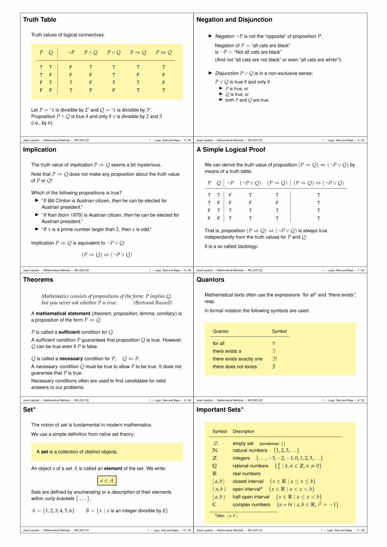
Truth Table
Truth values of logical connectives.
P Q ¬P P ∧Q P ∨Q P⇒ Q P⇔ Q
T T F T T T T
T F F F T F F
F T T F T T F
F F T F F T T
Let P = “x is divisible by 2” and Q = “x is divisible by 3”.Proposition P ∧Q is true if and only if x is divisible by 2 and 3(i.e., by 6).
Josef Leydold – Mathematical Methods – WS 2021/22 1 – Logic, Sets and Maps – 4 / 30
Negation and Disjunction
I Negation ¬P is not the “opposite” of proposition P.
Negation of P = “all cats are black”is ¬P = “Not all cats are black”
(And not “all cats are not black” or even “all cats are white”!)
I Disjunction P ∨Q is in a non-exclusive sense:
P ∨Q is true if and only ifI P is true, orI Q is true, orI both P and Q are true.
Josef Leydold – Mathematical Methods – WS 2021/22 1 – Logic, Sets and Maps – 5 / 30
Implication
The truth value of implication P⇒ Q seems a bit mysterious.
Note that P⇒ Q does not make any proposition about the truth valueof P or Q!
Which of the following propositions is true?I “If Bill Clinton is Austrian citizen, then he can be elected for
Austrian president.”I “If Karl (born 1970) is Austrian citizen, then he can be elected for
Austrian president.”I “If x is a prime number larger than 2, then x is odd.”
Implication P⇒ Q is equivalent to ¬P ∨Q:
(P⇒ Q)⇔ (¬P ∨Q)
Josef Leydold – Mathematical Methods – WS 2021/22 1 – Logic, Sets and Maps – 6 / 30
A Simple Logical Proof
We can derive the truth value of proposition (P⇒ Q)⇔ (¬P ∨Q) bymeans of a truth table:
P Q ¬P (¬P ∨Q) (P⇒ Q) (P⇒ Q)⇔ (¬P ∨Q)
T T F T T T
T F F F F T
F T T T T T
F F T T T T
That is, proposition (P⇒ Q)⇔ (¬P ∨Q) is always trueindependently from the truth values for P and Q.
It is a so called tautology.
Josef Leydold – Mathematical Methods – WS 2021/22 1 – Logic, Sets and Maps – 7 / 30
Theorems
Mathematics consists of propositions of the form: P implies Q,but you never ask whether P is true. (Bertrand Russell)
A mathematical statement (theorem, proposition, lemma, corollary ) isa proposition of the form P⇒ Q.
P is called a sufficient condition for Q.
A sufficient condition P guarantees that proposition Q is true. However,Q can be true even if P is false.
Q is called a necessary condition for P, Q⇐ P.
A necessary condition Q must be true to allow P to be true. It does notguarantee that P is true.
Necessary conditions often are used to find candidates for validanswers to our problems.
Josef Leydold – Mathematical Methods – WS 2021/22 1 – Logic, Sets and Maps – 8 / 30
Quantors
Mathematical texts often use the expressions “for all” and “there exists”,resp.
In formal notation the following symbols are used:
Quantor Symbol
for all ∀there exists a ∃there exists exactly one ∃!there does not exists @
Josef Leydold – Mathematical Methods – WS 2021/22 1 – Logic, Sets and Maps – 9 / 30
Set∗
The notion of set is fundamental in modern mathematics.
We use a simple definition from naïve set theory:
A set is a collection of distinct objects.
An object a of a set A is called an element of the set. We write:
a ∈ A
Sets are defined by enumerating or a description of their elementswithin curly brackets
. . .
.
A = 1, 2, 3, 4, 5, 6 B = x | x is an integer divisible by 2
Josef Leydold – Mathematical Methods – WS 2021/22 1 – Logic, Sets and Maps – 10 / 30
Important Sets∗
Symbol Description
∅ empty set sometimes: N natural numbers 1, 2, 3, . . .Z integers . . . ,−3,−2,−1, 0, 1, 2, 3, . . .Q rational numbers k
n | k, n ∈ Z, n 6= 0R real numbers
[ a, b ] closed interval x ∈ R | a ≤ x ≤ b( a, b ) open intervala x ∈ R | a < x < b[ a, b ) half-open interval x ∈ R | a ≤ x < bC complex numbers a + bi | a, b ∈ R, i2 = −1
aalso: ] a, b [
Josef Leydold – Mathematical Methods – WS 2021/22 1 – Logic, Sets and Maps – 11 / 30

Venn Diagram∗
We assume that all sets are subsets of some universal superset Ω.
Sets can be represented by Venn diagrams where Ω is a rectangleand sets are depicted as circles or ovals.
Ω
A
Josef Leydold – Mathematical Methods – WS 2021/22 1 – Logic, Sets and Maps – 12 / 30
Subset and Superset∗
Set A is a subset of B, A ⊆ B , if all elements of A also belong to B,
x ∈ A⇒ x ∈ B.
Ω
B
A ⊆ B
Vice versa, B is then called a superset of A, B ⊇ A .
Set A is a proper subset of B, A ⊂ B (or: A $ B),if A ⊆ B and A 6= B.
Josef Leydold – Mathematical Methods – WS 2021/22 1 – Logic, Sets and Maps – 13 / 30
Basic Set Operations∗
Symbol Definition Name
A ∩ B x|x ∈ A and x ∈ B intersection
A ∪ B x|x ∈ A or x ∈ B union
A \ B x|x ∈ A and x 6∈ B set-theoretic differencea
A Ω \ A complement
aalso: A− B
Two sets A and B are disjoint if A ∩ B = ∅.
Josef Leydold – Mathematical Methods – WS 2021/22 1 – Logic, Sets and Maps – 14 / 30
Basic Set Operations∗
Ω
A B
A∩ B
Ω
A B
A∪ B
Ω
A B
A \ B
Ω
AA
Josef Leydold – Mathematical Methods – WS 2021/22 1 – Logic, Sets and Maps – 15 / 30
Rules for Basic Operations∗
Rule Name
A ∪ A = A ∩ A = A Idempotence
A ∪∅ = A and A ∩∅ = ∅ Identity
(A ∪ B) ∪ C = A ∪ (B ∪ C) and
(A ∩ B) ∩ C = A ∩ (B ∩ C)Associativity
A ∪ B = B ∪ A and A ∩ B = B ∩ A Commutativity
A ∪ (B ∩ C) = (A ∪ B) ∩ (A ∪ C) and
A ∩ (B ∪ C) = (A ∩ B) ∪ (A ∩ C)Distributivity
A ∪ A = Ω and A ∩ A = ∅ and A = A
Josef Leydold – Mathematical Methods – WS 2021/22 1 – Logic, Sets and Maps – 16 / 30
De Morgan’s Law∗
(A ∪ B) = A ∩ B and (A ∩ B) = A ∪ B
Ω
A B
Ω
A B
A union B complemented is theequivalent of A complementedintersected with B complemented.
Josef Leydold – Mathematical Methods – WS 2021/22 1 – Logic, Sets and Maps – 17 / 30
Cartesian Product∗
The set
A× B = (x, y)|x ∈ A, y ∈ B
is called the Cartesian product of sets A and B.
Given two sets A and B the Cartesian product A× B is the set of allunique ordered pairs where the first element is from set A and thesecond element is from set B.
In general we have A× B 6= B× A.
Josef Leydold – Mathematical Methods – WS 2021/22 1 – Logic, Sets and Maps – 18 / 30
Cartesian Product∗
The Cartesian product of A = 0, 1 and B = 2, 3, 4 is
A× B = (0, 2), (0, 3), (0, 4), (1, 2), (1, 3), (1, 4).
A× B 2 3 40 (0, 2) (0, 3) (0, 4)1 (1, 2) (1, 3) (1, 4)
Josef Leydold – Mathematical Methods – WS 2021/22 1 – Logic, Sets and Maps – 19 / 30

Cartesian Product∗
The Cartesian product of A = [2, 4] and B = [1, 3] is
A× B = (x, y) | x ∈ [2, 4] and y ∈ [1, 3].
0 1 2 3 4
1
2
3
A = [2, 4]
B = [1, 3] A× B
Josef Leydold – Mathematical Methods – WS 2021/22 1 – Logic, Sets and Maps – 20 / 30
Map∗
A map (or mapping) f is defined by
(i) a domain D f ,
(ii) a codomain (target set) W f and
(iii) a rule, that maps each element of D to exactly one element of W.
f : D →W, x 7→ y = f (x)
I x is called the independent variable, y the dependent variable.I y is the image of x, x is the preimage of y.I f (x) is the function term, x is called the argument of f .I f (D) = y ∈W : y = f (x) for some x ∈ D
is the image (or range) of f .
Other names: function, transformation
Josef Leydold – Mathematical Methods – WS 2021/22 1 – Logic, Sets and Maps – 21 / 30
Injective · Surjective · Bijective∗
Each argument has exactly one image.Each y ∈W, however, may have any number of preimages.Thus we can characterize maps by their possible number of preimages.
I A map f is called one-to-one (or injective), if each element in thecodomain has at most one preimage.
I It is called onto (or surjective), if each element in the codomainhas at least one preimage.
I It is called bijective, if it is both one-to-one and onto, i.e., if eachelement in the codomain has exactly one preimage.
Injections have the important property
f (x) 6= f (y) ⇔ x 6= y
Josef Leydold – Mathematical Methods – WS 2021/22 1 – Logic, Sets and Maps – 22 / 30
Injective · Surjective · Bijective∗
Maps can be visualized by means of arrows.
D f W f D f W f D f W f
one-to-one onto one-to-one and onto
(not onto) (not one-to-one) (bijective)
Josef Leydold – Mathematical Methods – WS 2021/22 1 – Logic, Sets and Maps – 23 / 30
Function Composition∗
Let f : D f →W f and g : Dg →Wg be functions with W f ⊆ Dg.
Function
g f : D f →Wg, x 7→ (g f )(x) = g( f (x))
is called composite function.(read: “g composed with f ”, “g circle f ”, or “g after f ”)
D f W f ⊆ Dg Wg
f g
g f
Josef Leydold – Mathematical Methods – WS 2021/22 1 – Logic, Sets and Maps – 24 / 30
Inverse Map∗
If f : D f →W f is a bijection, then every y ∈W f can be uniquelymapped to its preimage x ∈ D f .
Thus we get a map
f−1 : W f → D f , y 7→ x = f−1(y)
which is called the inverse map of f .
We obviously have for all x ∈ D f and y ∈W f ,
f−1( f (x)) = f−1(y) = x and f ( f−1(y)) = f (x) = y .
Josef Leydold – Mathematical Methods – WS 2021/22 1 – Logic, Sets and Maps – 25 / 30
Inverse Map∗
D fW f−1
W fD f−1
f
f−1
Josef Leydold – Mathematical Methods – WS 2021/22 1 – Logic, Sets and Maps – 26 / 30
Identity∗
The most elementary function is the identity map id,which maps its argument to itself, i.e.,
id : D →W = D, x 7→ x
D
1234
W = D
1234
id
Josef Leydold – Mathematical Methods – WS 2021/22 1 – Logic, Sets and Maps – 27 / 30
Identity∗
The identity map has a similar role for compositions of functions as 1has for multiplications of numbers:
f id = f and id f = f
Moreover,
f−1 f = id : D f → D f and f f−1 = id : W f →W f
Josef Leydold – Mathematical Methods – WS 2021/22 1 – Logic, Sets and Maps – 28 / 30
Real-valued Functions∗
Maps where domain and codomain are (subsets of) real numbers arecalled real-valued functions,
f : R→ R, x 7→ f (x)
and are the most important kind of functions.
The term function is often exclusively used for real-valued maps.
We will discuss such functions in more details later.
Josef Leydold – Mathematical Methods – WS 2021/22 1 – Logic, Sets and Maps – 29 / 30
Summary
I mathematical logicI theoremI necessary and sufficient conditionI sets, subsets and supersetsI Venn diagramI basic set operationsI de Morgan’s lawI Cartesian productI mapsI one-to-one and ontoI inverse map and identity
Josef Leydold – Mathematical Methods – WS 2021/22 1 – Logic, Sets and Maps – 30 / 30
Chapter 2
Matrix Algebra
Josef Leydold – Mathematical Methods – WS 2021/22 2 – Matrix Algebra – 1 / 36
A Very Simplistic Leontief Model
A community operates the services PUBLIC TRANSPORT, ELECTRICITY
and GAS.
Technology matrix and weekly demand (in unit values):
expenditure of
fortransport electricity gas demand
transport 0.0 0.2 0.2 7.0
electricity 0.4 0.2 0.1 12.5
gas 0.0 0.5 0.1 16.5
What is the weekly production that satisfies the demand(but does not create excess)?
Josef Leydold – Mathematical Methods – WS 2021/22 2 – Matrix Algebra – 2 / 36
A Very Simplistic Leontief Model
We denote the unknown units of production of TRANSPORT,ELECTRICITY and GAS by x1, x2,and x3, resp.For our production we must have:
demand = production − internal expenditur
7.0 = x1 − (0.0 x1 + 0.2 x2 + 0.2 x3)
12.5 = x2 − (0.4 x1 + 0.2 x2 + 0.1 x3)
16.5 = x3 − (0.0 x1 + 0.5 x2 + 0.1 x3)
Transformation into an equivalent system of equations yields:
1.0 x1 − 0.2 x2 − 0.2 x3 = 7.0−0.4 x1 + 0.8 x2 − 0.1 x3 = 12.5
0.0 x1 − 0.5 x2 + 0.9 x3 = 16.5
Which values for x1, x2, and x3 solves these equations simultaneously?
Josef Leydold – Mathematical Methods – WS 2021/22 2 – Matrix Algebra – 3 / 36
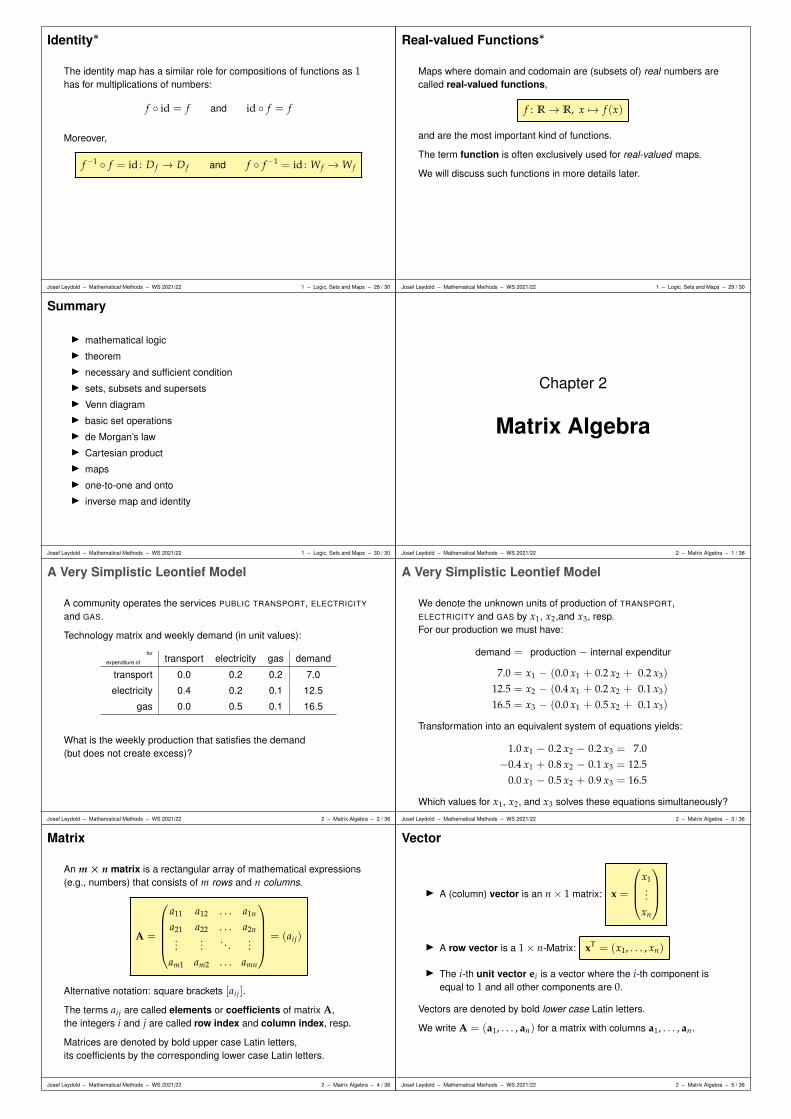
Matrix
An m× n matrix is a rectangular array of mathematical expressions(e.g., numbers) that consists of m rows and n columns.
A =
a11 a12 . . . a1n
a21 a22 . . . a2n...
.... . .
...
am1 am2 . . . amn
= (aij)
Alternative notation: square brackets [aij].
The terms aij are called elements or coefficients of matrix A,the integers i and j are called row index and column index, resp.
Matrices are denoted by bold upper case Latin letters,its coefficients by the corresponding lower case Latin letters.
Josef Leydold – Mathematical Methods – WS 2021/22 2 – Matrix Algebra – 4 / 36
Vector
I A (column) vector is an n× 1 matrix: x =
x1...
xn
I A row vector is a 1× n-Matrix: xT = (x1, . . . , xn)
I The i-th unit vector ei is a vector where the i-th component isequal to 1 and all other components are 0.
Vectors are denoted by bold lower case Latin letters.
We write A = (a1, . . . , an) for a matrix with columns a1, . . . , an.
Josef Leydold – Mathematical Methods – WS 2021/22 2 – Matrix Algebra – 5 / 36

Elements of a Matrix
We use the symbol
[A]
ij = aij
to denote the coefficient with respective row and column index i and j.
The convenient symbol
δij =
1, if i = j,0, if i 6= j.
is called the Kronecker symbol.
Example of its usage: [I]ij = δij.
Josef Leydold – Mathematical Methods – WS 2021/22 2 – Matrix Algebra – 6 / 36
Special Matrices
I An n× n matrix is called square matrix.
I An upper triangular matrix is a square matrix where all elementsbelow the main diagonal are zero.
U =
−1 −3 10 2 30 0 −2
Formally:Matrix U is an upper triangular matrix if
[U]ij = 0 whenever i > j.
Josef Leydold – Mathematical Methods – WS 2021/22 2 – Matrix Algebra – 7 / 36
Special Matrices
I A lower triangular matrix is a square matrix where all elementsabove the main diagonal are zero.
L =
1 0 02 3 00 4 0
Formally:Matrix L is a lower triangular matrix if
[L]ij = 0 whenever i < j.
Josef Leydold – Mathematical Methods – WS 2021/22 2 – Matrix Algebra – 8 / 36
Special Matrices
I A diagonal matrix is a square matrix where all elements outsidethe main diagonal are zero.
D =
1 0 00 2 00 0 3
Formally:Matrix D is a diagonal matrix if
[D]ij = 0 whenever i 6= j.
Josef Leydold – Mathematical Methods – WS 2021/22 2 – Matrix Algebra – 9 / 36
Special Matrices
I A matrix where all its coefficients are zero is called a zero matrixand is denoted by On,m or 0.
I An identity matrix is a diagonal matrix where all its diagonalentries are equal to 1. It is denoted by In or I.(In German literature also symbol E is used.)
I3 =
1 0 00 1 00 0 1
Remark: Both identity matrix In and zero matrix On,n are examples ofupper and lower triangular matrices and of a diagonal matrix.
Josef Leydold – Mathematical Methods – WS 2021/22 2 – Matrix Algebra – 10 / 36
Transposed Matrix
We get the transposed AT of matrix A by exchanging rows andcolumns:
[AT]
ij= [A]ji
(1 2 34 5 6
)T
=
1 42 53 6
Alternative notation: A′
Josef Leydold – Mathematical Methods – WS 2021/22 2 – Matrix Algebra – 11 / 36
Symmetric Matrix
A matrix A is called symmetric if
AT = A
i.e., if
[A]ij = [A]ji for all i, j.
Obviously every symmetric matrix is a square matrix.
Matrix
1 2 32 4 53 5 6
is symmetric.
Josef Leydold – Mathematical Methods – WS 2021/22 2 – Matrix Algebra – 12 / 36
Scalar Multiplication
A matrix A can be multiplied by a constant (scalar) α ∈ R
component-wise:
[α ·A]ij = α [A]ij
3 ·(
1 23 4
)=
(3 69 12
)
Josef Leydold – Mathematical Methods – WS 2021/22 2 – Matrix Algebra – 13 / 36
Addition of Matrices
Two m× n matrices A and B are added component-wise:
[A + B]ij = [A]ij + [B]ij
Addition of two matrices is only possible if their numbers of rows andcolumns coincide!
(1 23 4
)+
(5 67 8
)=
(1 + 5 2 + 63 + 7 4 + 8
)=
(6 810 12
)
Josef Leydold – Mathematical Methods – WS 2021/22 2 – Matrix Algebra – 14 / 36
Multiplication of Matrices
The product A · B of two matrices A and B is defined only if thenumber of columns of the first factor A coincides with the number ofrows of the second factor B.
That is, if A is an m× n matrix, then B must be an n× k matrix.The product C = A · B then is an m× k matrix.
Element [A · B]ij is then the product of the ith row of A and the jthcolumn of B (in the sense of a scalar product):
[A · B]ij =n
∑s=1
ais · bsj
Matrix multiplication is not commutative!
Josef Leydold – Mathematical Methods – WS 2021/22 2 – Matrix Algebra – 15 / 36
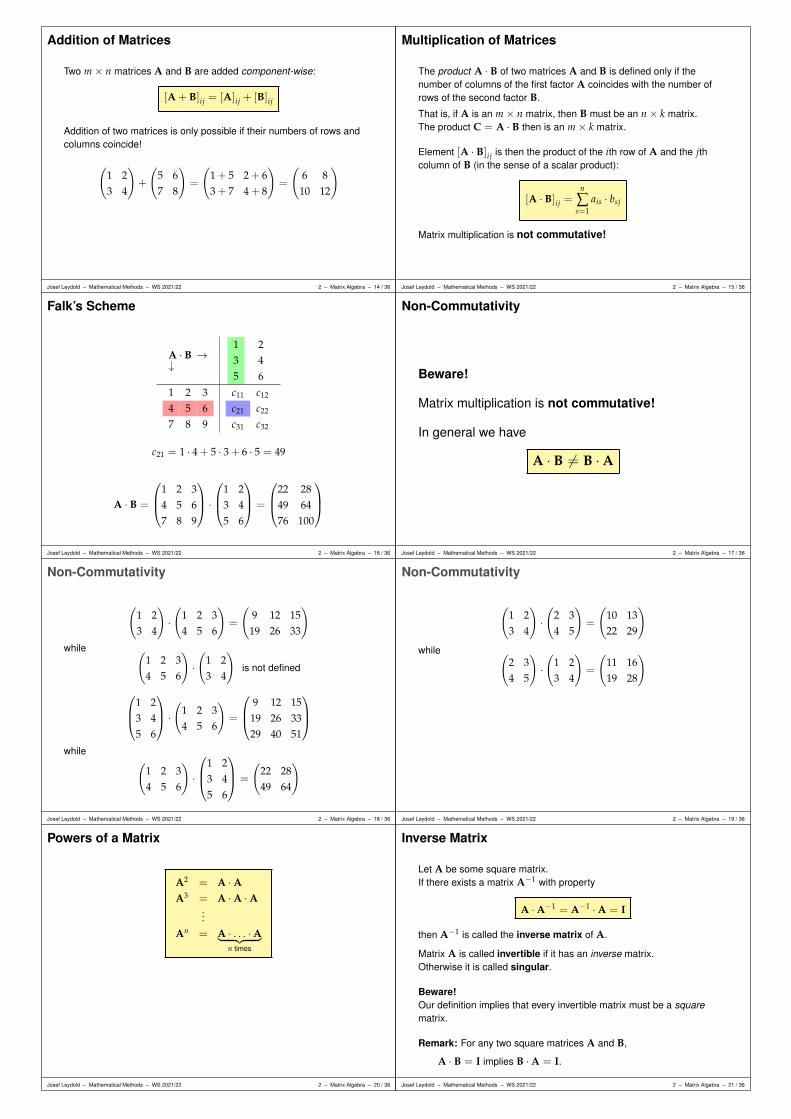
Falk’s Scheme
A · B →↓
1 23 45 6
1 2 34 5 67 8 9
c11 c12
c21 c22
c31 c32
c21 = 1 · 4 + 5 · 3 + 6 · 5 = 49
A · B =
1 2 34 5 67 8 9
·
1 23 45 6
=
22 2849 6476 100
Josef Leydold – Mathematical Methods – WS 2021/22 2 – Matrix Algebra – 16 / 36
Non-Commutativity
Beware!
Matrix multiplication is not commutative!
In general we have
A · B 6= B ·A
Josef Leydold – Mathematical Methods – WS 2021/22 2 – Matrix Algebra – 17 / 36
Non-Commutativity
(1 23 4
)·(
1 2 34 5 6
)=
(9 12 1519 26 33
)
while (1 2 34 5 6
)·(
1 23 4
)is not defined
1 23 45 6
·
(1 2 34 5 6
)=
9 12 1519 26 3329 40 51
while(
1 2 34 5 6
)·
1 23 45 6
=
(22 2849 64
)
Josef Leydold – Mathematical Methods – WS 2021/22 2 – Matrix Algebra – 18 / 36
Non-Commutativity
(1 23 4
)·(
2 34 5
)=
(10 1322 29
)
while (2 34 5
)·(
1 23 4
)=
(11 1619 28
)
Josef Leydold – Mathematical Methods – WS 2021/22 2 – Matrix Algebra – 19 / 36
Powers of a Matrix
A2 = A ·AA3 = A ·A ·A
...
An = A · . . . ·A︸ ︷︷ ︸n times
Josef Leydold – Mathematical Methods – WS 2021/22 2 – Matrix Algebra – 20 / 36
Inverse Matrix
Let A be some square matrix.If there exists a matrix A−1 with property
A ·A−1 = A−1 ·A = I
then A−1 is called the inverse matrix of A.
Matrix A is called invertible if it has an inverse matrix.Otherwise it is called singular.
Beware!Our definition implies that every invertible matrix must be a squarematrix.
Remark: For any two square matrices A and B,
A · B = I implies B ·A = I.
Josef Leydold – Mathematical Methods – WS 2021/22 2 – Matrix Algebra – 21 / 36
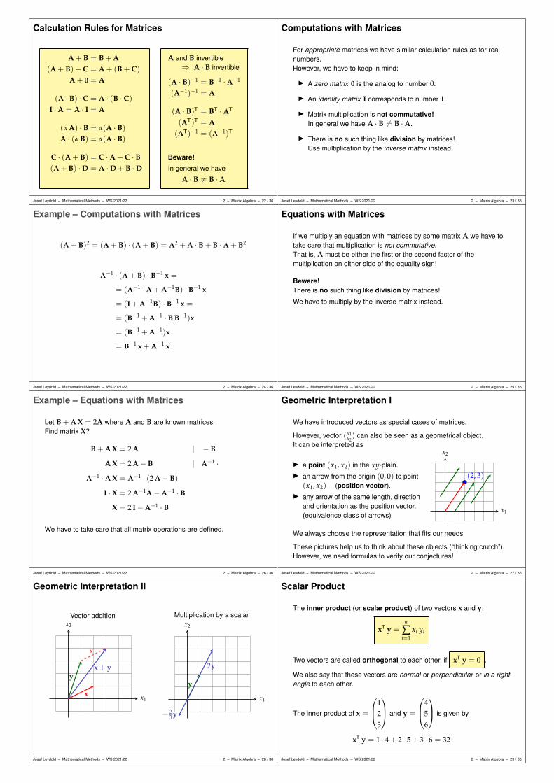
Calculation Rules for Matrices
A + B = B + A(A + B) + C = A + (B + C)
A + 0 = A
(A · B) · C = A · (B · C)
I ·A = A · I = A
(α A) · B = α(A · B)A · (α B) = α(A · B)
C · (A + B) = C ·A + C · B(A + B) ·D = A ·D + B ·D
A and B invertible⇒ A · B invertible
(A · B)−1 = B−1 ·A−1
(A−1)−1 = A
(A · B)T = BT ·AT
(AT)T = A(AT)−1 = (A−1)T
Beware!
In general we have
A · B 6= B ·A
Josef Leydold – Mathematical Methods – WS 2021/22 2 – Matrix Algebra – 22 / 36
Computations with Matrices
For appropriate matrices we have similar calculation rules as for realnumbers.However, we have to keep in mind:
I A zero matrix 0 is the analog to number 0.
I An identity matrix I corresponds to number 1.
I Matrix multiplication is not commutative!In general we have A · B 6= B ·A.
I There is no such thing like division by matrices!Use multiplication by the inverse matrix instead.
Josef Leydold – Mathematical Methods – WS 2021/22 2 – Matrix Algebra – 23 / 36
Example – Computations with Matrices
(A + B)2 = (A + B) · (A + B) = A2 + A · B + B ·A + B2
A−1 · (A + B) · B−1 x =
= (A−1 ·A + A−1B) · B−1 x
= (I + A−1B) · B−1 x =
= (B−1 + A−1 · B B−1)x
= (B−1 + A−1)x
= B−1 x + A−1 x
Josef Leydold – Mathematical Methods – WS 2021/22 2 – Matrix Algebra – 24 / 36
Equations with Matrices
If we multiply an equation with matrices by some matrix A we have totake care that multiplication is not commutative.That is, A must be either the first or the second factor of themultiplication on either side of the equality sign!
Beware!There is no such thing like division by matrices!
We have to multiply by the inverse matrix instead.
Josef Leydold – Mathematical Methods – WS 2021/22 2 – Matrix Algebra – 25 / 36
Example – Equations with Matrices
Let B + A X = 2A where A and B are known matrices.Find matrix X?
B + A X = 2 A | − B
A X = 2 A− B | A−1 ·A−1 ·A X = A−1 · (2 A− B)
I · X = 2 A−1A−A−1 · BX = 2 I−A−1 · B
We have to take care that all matrix operations are defined.
Josef Leydold – Mathematical Methods – WS 2021/22 2 – Matrix Algebra – 26 / 36
Geometric Interpretation I
We have introduced vectors as special cases of matrices.
However, vector (x1x2) can also be seen as a geometrical object.
It can be interpreted as
I a point (x1, x2) in the xy-plain.I an arrow from the origin (0, 0) to point
(x1, x2) (position vector).I any arrow of the same length, direction
and orientation as the position vector.(equivalence class of arrows)
x1
x2
(2, 3)
We always choose the representation that fits our needs.
These pictures help us to think about these objects (“thinking crutch”).However, we need formulas to verify our conjectures!
Josef Leydold – Mathematical Methods – WS 2021/22 2 – Matrix Algebra – 27 / 36
Geometric Interpretation II
Vector addition
x1
x2
x
y
x
x + y
Multiplication by a scalar
x1
x2
y
2y
− 23 y
Josef Leydold – Mathematical Methods – WS 2021/22 2 – Matrix Algebra – 28 / 36
Scalar Product
The inner product (or scalar product) of two vectors x and y:
xT y =n
∑i=1
xi yi
Two vectors are called orthogonal to each other, if xT y = 0 .
We also say that these vectors are normal or perpendicular or in a rightangle to each other.
The inner product of x =
123
and y =
456
is given by
xT y = 1 · 4 + 2 · 5 + 3 · 6 = 32
Josef Leydold – Mathematical Methods – WS 2021/22 2 – Matrix Algebra – 29 / 36

Norm
The (Euclidean) norm ‖x‖ of vector x:
‖x‖ =√
xT x =
√n
∑i=1
x2i
A vector x is called normalized, if ‖x‖ = 1.
The norm of x =
123
is given by
‖x‖ =√
12 + 22 + 32 =√
14
Josef Leydold – Mathematical Methods – WS 2021/22 2 – Matrix Algebra – 30 / 36
Geometric Interpretation
The norm of a vector can be interpreted as its length:
‖x‖2
x21
x22
Pythagorean theorem:
‖x‖2 = x21 + x2
2
The inner product measures angles between two vectors:
cos^(x, y) =xT y
‖x‖ · ‖y‖
Josef Leydold – Mathematical Methods – WS 2021/22 2 – Matrix Algebra – 31 / 36
Properties of the Norm
(i) ‖x‖ ≥ 0.
(ii) ‖x‖ = 0 ⇔ x = 0.
(iii) ‖αx‖ = |α| · ‖x‖ for all α ∈ R.
(iv) ‖x + y‖ ≤ ‖x‖+ ‖y‖. (Triangle inequality)
Josef Leydold – Mathematical Methods – WS 2021/22 2 – Matrix Algebra – 32 / 36
Inequalities
I Cauchy-Schwarz inequality
|xTy| ≤ ‖x‖ · ‖y‖
I Minkowski inequality (triangle inequality)
‖x + y‖ ≤ ‖x‖+ ‖y‖
I Pythagorean theorem
For orthogonal vectors x and y we have
‖x + y‖2 = ‖x‖2 + ‖y‖2
Josef Leydold – Mathematical Methods – WS 2021/22 2 – Matrix Algebra – 33 / 36
Leontief Model
A . . . technology matrix
x . . . production vector
b . . . demand vector
p . . . prices for goods
w . . . wages
Prices must cover production costs:
pj = ∑ni=1 aij pi + wj = a1j p1 + a2j p2 + · · ·+ anj pn + wj
p = ATp + w
So for fixed wages we find:
p = (I−AT)−1w
Moreover, for the input-output model we have:
x = Ax + b
Josef Leydold – Mathematical Methods – WS 2021/22 2 – Matrix Algebra – 34 / 36
Leontief Model
Demand is given by the wages for produced goods:
demand = w1x1 + w2x2 + · · ·+ wnxn = wTx
Supply is given by prices for demanded goods:
supply = p1b1 + p2b2 + · · ·+ pnbn = pTb
If the following equations hold in a input-output model
x = Ax + b and p = ATp + w
then we have market equilibrium, i.e., wTx = pTb.
Proof:
wTx = (pT − pTA)x = pT(I−A)x = pT(x−Ax) = pTb
Josef Leydold – Mathematical Methods – WS 2021/22 2 – Matrix Algebra – 35 / 36
Summary
I matrix and vectorI triangular and diagonal matrixI zero matrix and identity matrixI transposed and symmetric matrixI inverse matrixI computations with matrices (matrix algebra)I equations with matricesI norm and inner product of vectors
Josef Leydold – Mathematical Methods – WS 2021/22 2 – Matrix Algebra – 36 / 36
Chapter 3
Linear Equations
Josef Leydold – Mathematical Methods – WS 2021/22 3 – Linear Equations – 1 / 33
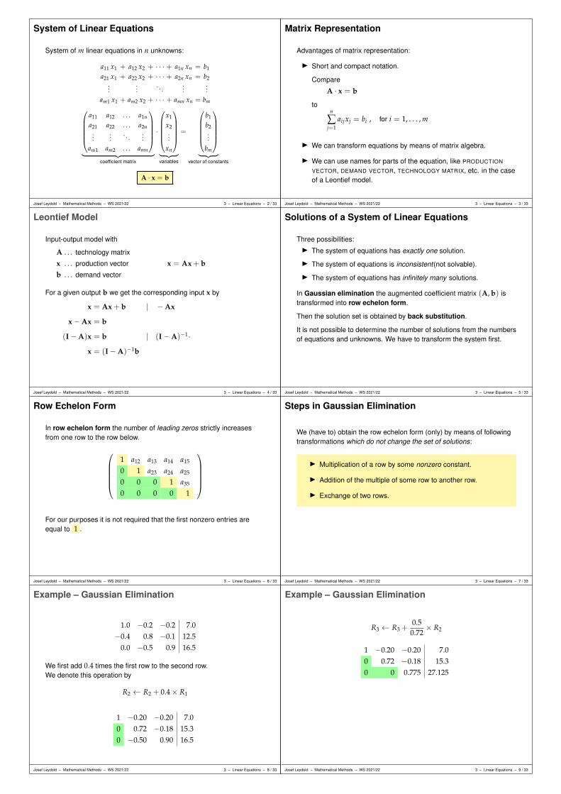
System of Linear Equations
System of m linear equations in n unknowns:
a11 x1 + a12 x2 + · · · + a1n xn = b1
a21 x1 + a22 x2 + · · · + a2n xn = b2...
.... . .
......
am1 x1 + am2 x2 + · · · + amn xn = bm
a11 a12 . . . a1n
a21 a22 . . . a2n...
.... . .
...
am1 am2 . . . amn
︸ ︷︷ ︸coefficient matrix
·
x1
x2...
xn
︸ ︷︷ ︸variables
=
b1
b2...
bm
︸ ︷︷ ︸vector of constants
A · x = b
Josef Leydold – Mathematical Methods – WS 2021/22 3 – Linear Equations – 2 / 33
Matrix Representation
Advantages of matrix representation:
I Short and compact notation.
Compare
A · x = b
ton
∑j=1
aijxj = bi , for i = 1, . . . , m
I We can transform equations by means of matrix algebra.
I We can use names for parts of the equation, like PRODUCTION
VECTOR, DEMAND VECTOR, TECHNOLOGY MATRIX, etc. in the caseof a Leontief model.
Josef Leydold – Mathematical Methods – WS 2021/22 3 – Linear Equations – 3 / 33
Leontief Model
Input-output model with
A . . . technology matrix
x . . . production vector x = Ax + bb . . . demand vector
For a given output b we get the corresponding input x by
x = Ax + b | −Ax
x−Ax = b
(I−A)x = b | (I−A)−1·x = (I−A)−1b
Josef Leydold – Mathematical Methods – WS 2021/22 3 – Linear Equations – 4 / 33
Solutions of a System of Linear Equations
Three possibilities:I The system of equations has exactly one solution.
I The system of equations is inconsistent(not solvable).
I The system of equations has infinitely many solutions.
In Gaussian elimination the augmented coefficient matrix (A, b) istransformed into row echelon form.
Then the solution set is obtained by back substitution.
It is not possible to determine the number of solutions from the numbersof equations and unknowns. We have to transform the system first.
Josef Leydold – Mathematical Methods – WS 2021/22 3 – Linear Equations – 5 / 33
Row Echelon Form
In row echelon form the number of leading zeros strictly increasesfrom one row to the row below.
1 a12 a13 a14 a15
0 1 a23 a24 a25
0 0 0 1 a35
0 0 0 0 1
For our purposes it is not required that the first nonzero entries areequal to 1 .
Josef Leydold – Mathematical Methods – WS 2021/22 3 – Linear Equations – 6 / 33
Steps in Gaussian Elimination
We (have to) obtain the row echelon form (only) by means of followingtransformations which do not change the set of solutions:
I Multiplication of a row by some nonzero constant.
I Addition of the multiple of some row to another row.
I Exchange of two rows.
Josef Leydold – Mathematical Methods – WS 2021/22 3 – Linear Equations – 7 / 33
Example – Gaussian Elimination
1.0 −0.2 −0.2 7.0−0.4 0.8 −0.1 12.5
0.0 −0.5 0.9 16.5
We first add 0.4 times the first row to the second row.We denote this operation by
R2 ← R2 + 0.4× R1
1 −0.20 −0.20 7.00 0.72 −0.18 15.30 −0.50 0.90 16.5
Josef Leydold – Mathematical Methods – WS 2021/22 3 – Linear Equations – 8 / 33
Example – Gaussian Elimination
R3 ← R3 +0.5
0.72× R2
1 −0.20 −0.20 7.00 0.72 −0.18 15.30 0 0.775 27.125
Josef Leydold – Mathematical Methods – WS 2021/22 3 – Linear Equations – 9 / 33

Example – Back Substitution
1 −0.20 −0.20 7.00 0.72 −0.18 15.30 0 0.775 27.125
From the third row we immediately get:
0.775 · x3 = 27.125 ⇒ x3 = 35
We obtain the remaining variables x2 and x1 by back substitution:
0.72 · x2 − 0.18 · 35 = 15.3 ⇒ x2 = 30
x1 − 0.2 · 30− 0.2 · 35 = 7 ⇒ x1 = 20
The solution is unique: x = (20, 30, 35)T
Josef Leydold – Mathematical Methods – WS 2021/22 3 – Linear Equations – 10 / 33
Example 2
Find the solution of equation
3 x1 + 4 x2 + 5 x3 = 1x1 + x2 − x3 = 2
5 x1 + 6 x2 + 3 x3 = 4
3 4 5 11 1 −1 25 6 3 4
R2 ← 3× R2 − R1, R3 ← 3× R3 − 5× R1
3 4 5 10 −1 −8 50 −2 −16 7
Josef Leydold – Mathematical Methods – WS 2021/22 3 – Linear Equations – 11 / 33
Example 2
R3 ← R3 − 2× R2
3 4 5 10 −1 −8 50 0 0 −3
The third row implies 0 = −3 , a contradiction.
This system of equations is inconsistent; solution set L = ∅.
Josef Leydold – Mathematical Methods – WS 2021/22 3 – Linear Equations – 12 / 33
Example 3
Find the solution of equation
2 x1 + 8 x2 + 10 x3 + 10 x4 = 0x1 + 5 x2 + 2 x3 + 9 x4 = 1
−3 x1 − 10 x2 − 21 x3 − 6 x4 = −4
2 8 10 10 01 5 2 9 1−3 −10 −21 −6 −4
R2 ← 2× R2 − R1, R3 ← 2× R3 + 3× R1
2 8 10 10 00 2 −6 8 20 4 −12 18 −8
Josef Leydold – Mathematical Methods – WS 2021/22 3 – Linear Equations – 13 / 33
Example 3
R3 ← R3 − 2× R2
2 8 10 10 00 2 −6 8 20 0 0 2 −12
This equation has infinitely many solutions.This can be seen from the row echelon form as there are morevariables than nonzero rows.
Josef Leydold – Mathematical Methods – WS 2021/22 3 – Linear Equations – 14 / 33
Example 3
The third row immediately implies
2 · x4 = −12 ⇒ x4 = −6
Back substitution yields
2 · x2 − 6 · x3 + 8 · (−6) = 2
In this case we use pseudo solution x3 = α , α ∈ R, and get
x2 − 3 · α + 4 · (−6) = 1 ⇒ x2 = 25 + 3 α
2 · x1 + 8 · (25 + 3 · α) + 10 · α + 10 · (−6) = 0
⇒ x1 = −70− 17 · α
Josef Leydold – Mathematical Methods – WS 2021/22 3 – Linear Equations – 15 / 33
Example 3
We obtain a solution for each value of α. Using vector notation weobtain
x =
x1
x2
x3
x4
=
−70− 17 · α
25 + 3 α
α
−6
=
−70250−6
+ α
−17310
Thus the solution set of this equation is
L =
x =
−70250−6
+ α
−17310
∣∣∣∣∣∣∣∣∣∣
α ∈ R
Josef Leydold – Mathematical Methods – WS 2021/22 3 – Linear Equations – 16 / 33
Equivalent Representation of Solutions
In Example 3 we also could use x2 = α′ (instead of x3 = α).Then back substitution yields
L′ =
x =
x1
x2
x3
x4
=
− 2153
0− 25
3
−6
+ α′
− 173
113
0
∣∣∣∣∣∣∣∣∣∣
α ∈ R
However, these two solution sets are equal, L′ = L!
We thus have two different – but equivalent – representations of thesame set.
The solution set is unique, its representation is not!
Josef Leydold – Mathematical Methods – WS 2021/22 3 – Linear Equations – 17 / 33
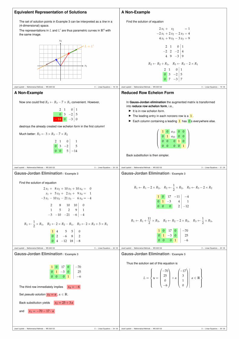
Equivalent Representation of Solutions
The set of solution points in Example 3 can be interpreted as a line in a(4-dimensional) space.
The representations in L and L′ are thus parametric curves in R4 withthe same image.
x1
x2
L = L′
Josef Leydold – Mathematical Methods – WS 2021/22 3 – Linear Equations – 18 / 33
A Non-Example
Find the solution of equation
2 x1 + x2 = 1−2 x1 + 2 x2 − 2 x3 = 4
4 x1 + 9 x2 − 3 x3 = 9
2 1 0 1−2 2 −2 4
4 9 −3 9
R2 ← R2 + R1, R3 ← R3 − 2× R1
2 1 0 10 3 −2 50 7 −3 7
Josef Leydold – Mathematical Methods – WS 2021/22 3 – Linear Equations – 19 / 33
A Non-Example
Now one could find R3 ← R3 − 7× R1 convenient. However,
2 1 0 10 3 −2 5
−14 0 −3 0
destroys the already created row echelon form in the first column!
Much better: R3 ← 3× R3 − 7× R2
2 1 0 10 3 −2 50 0 5 −14
Josef Leydold – Mathematical Methods – WS 2021/22 3 – Linear Equations – 20 / 33
Reduced Row Echelon Form
In Gauss-Jordan elimination the augmented matrix is transformedinto reduce row echelon form, i.e.,I It is in row echelon form.I The leading entry in each nonzero row is a 1 .
I Each column containing a leading 1 has 0 s everywhere else.
1 0 a13 0 00 1 a23 0 00 0 0 1 00 0 0 0 1
Back substitution is then simpler.
Josef Leydold – Mathematical Methods – WS 2021/22 3 – Linear Equations – 21 / 33
Gauss-Jordan Elimination / Example 3
Find the solution of equation
2 x1 + 8 x2 + 10 x3 + 10 x4 = 0x1 + 5 x2 + 2 x3 + 9 x4 = 1
−3 x1 − 10 x2 − 21 x3 − 6 x4 = −4
2 8 10 10 01 5 2 9 1−3 −10 −21 −6 −4
R1 ←12× R1, R2 ← 2× R2 − R1, R3 ← 2× R3 + 3× R1
1 4 5 5 00 2 −6 8 20 4 −12 18 −8
Josef Leydold – Mathematical Methods – WS 2021/22 3 – Linear Equations – 22 / 33
Gauss-Jordan Elimination / Example 3
R1 ← R1 − 2× R2, R2 ←12× R2, R3 ← R3 − 2× R2
1 0 17 −11 −40 1 −3 4 10 0 0 2 −12
R1 ← R1 +112× R3, R2 ← R2 − 2× R3, R3 ←
12× R3,
1 0 17 0 −700 1 −3 0 250 0 0 1 −6
Josef Leydold – Mathematical Methods – WS 2021/22 3 – Linear Equations – 23 / 33
Gauss-Jordan Elimination / Example 3
1 0 17 0 −700 1 −3 0 250 0 0 1 −6
The third row immediately implies x4 = −6
Set pseudo solution x3 = α , α ∈ R.
Back substitution yields x2 = 25 + 3 α
and x1 = −70− 17 · α
Josef Leydold – Mathematical Methods – WS 2021/22 3 – Linear Equations – 24 / 33
Gauss-Jordan Elimination / Example 3
Thus the solution set of this equation is
L =
x =
−70250−6
+ α
−17310
∣∣∣∣∣∣∣∣∣∣
α ∈ R
Josef Leydold – Mathematical Methods – WS 2021/22 3 – Linear Equations – 25 / 33
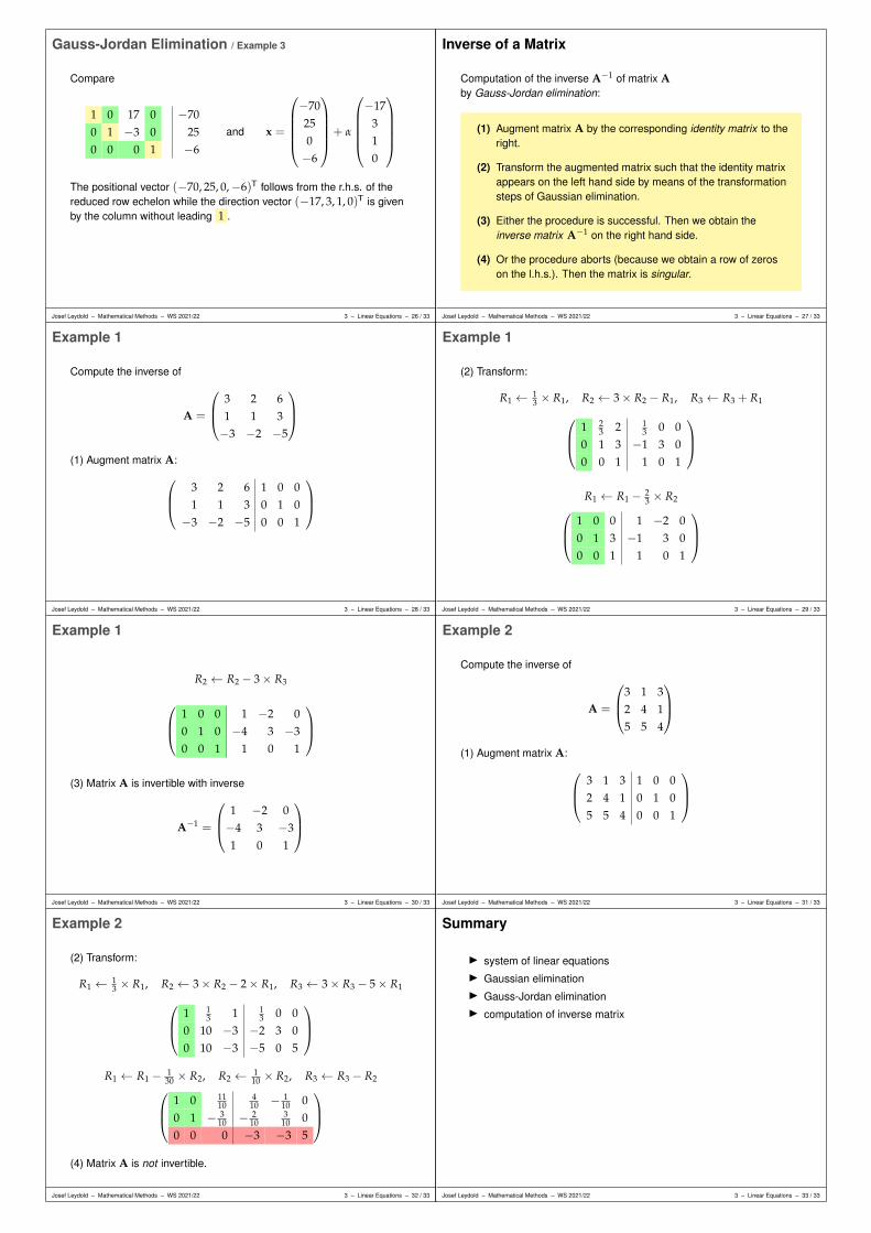
Gauss-Jordan Elimination / Example 3
Compare
1 0 17 0 −700 1 −3 0 250 0 0 1 −6
and x =
−70250−6
+ α
−17310
The positional vector (−70, 25, 0,−6)T follows from the r.h.s. of thereduced row echelon while the direction vector (−17, 3, 1, 0)T is givenby the column without leading 1 .
Josef Leydold – Mathematical Methods – WS 2021/22 3 – Linear Equations – 26 / 33
Inverse of a Matrix
Computation of the inverse A−1 of matrix Aby Gauss-Jordan elimination:
(1) Augment matrix A by the corresponding identity matrix to theright.
(2) Transform the augmented matrix such that the identity matrixappears on the left hand side by means of the transformationsteps of Gaussian elimination.
(3) Either the procedure is successful. Then we obtain theinverse matrix A−1 on the right hand side.
(4) Or the procedure aborts (because we obtain a row of zeroson the l.h.s.). Then the matrix is singular.
Josef Leydold – Mathematical Methods – WS 2021/22 3 – Linear Equations – 27 / 33
Example 1
Compute the inverse of
A =
3 2 61 1 3−3 −2 −5
(1) Augment matrix A:
3 2 6 1 0 01 1 3 0 1 0−3 −2 −5 0 0 1
Josef Leydold – Mathematical Methods – WS 2021/22 3 – Linear Equations – 28 / 33
Example 1
(2) Transform:
R1 ← 13 × R1, R2 ← 3× R2 − R1, R3 ← R3 + R1
1 23 2 1
3 0 00 1 3 −1 3 00 0 1 1 0 1
R1 ← R1 − 23 × R2
1 0 0 1 −2 00 1 3 −1 3 00 0 1 1 0 1
Josef Leydold – Mathematical Methods – WS 2021/22 3 – Linear Equations – 29 / 33
Example 1
R2 ← R2 − 3× R3
1 0 0 1 −2 00 1 0 −4 3 −30 0 1 1 0 1
(3) Matrix A is invertible with inverse
A−1 =
1 −2 0−4 3 −31 0 1
Josef Leydold – Mathematical Methods – WS 2021/22 3 – Linear Equations – 30 / 33
Example 2
Compute the inverse of
A =
3 1 32 4 15 5 4
(1) Augment matrix A:
3 1 3 1 0 02 4 1 0 1 05 5 4 0 0 1
Josef Leydold – Mathematical Methods – WS 2021/22 3 – Linear Equations – 31 / 33
Example 2
(2) Transform:
R1 ← 13 × R1, R2 ← 3× R2 − 2× R1, R3 ← 3× R3 − 5× R1
1 13 1 1
3 0 00 10 −3 −2 3 00 10 −3 −5 0 5
R1 ← R1 − 130 × R2, R2 ← 1
10 × R2, R3 ← R3 − R2
1 0 1110
410 − 1
10 00 1 − 3
10 − 210
310 0
0 0 0 −3 −3 5
(4) Matrix A is not invertible.
Josef Leydold – Mathematical Methods – WS 2021/22 3 – Linear Equations – 32 / 33
Summary
I system of linear equationsI Gaussian eliminationI Gauss-Jordan eliminationI computation of inverse matrix
Josef Leydold – Mathematical Methods – WS 2021/22 3 – Linear Equations – 33 / 33
Chapter 4
Vector Space
Josef Leydold – Mathematical Methods – WS 2021/22 4 – Vector Space – 1 / 54
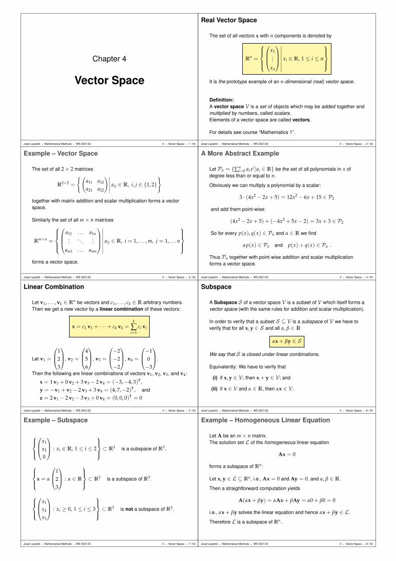
Real Vector Space
The set of all vectors x with n components is denoted by
Rn =
x1...
xn
∣∣∣∣∣∣∣∣xi ∈ R, 1 ≤ i ≤ n
It is the prototype example of an n-dimensional (real) vector space.
Definition:A vector space V is a set of objects which may be added together andmultiplied by numbers, called scalars.Elements of a vector space are called vectors.
For details see course “Mathematics 1”.
Josef Leydold – Mathematical Methods – WS 2021/22 4 – Vector Space – 2 / 54
Example – Vector Space
The set of all 2× 2 matrices
R2×2 =
(a11 a12
a21 a22
)∣∣∣∣∣ aij ∈ R, i, j ∈ 1, 2
together with matrix addition and scalar multiplication forms a vectorspace.
Similarly the set of all m× n matrices
Rm×n =
a11 . . . a1n...
. . ....
am1 . . . amn
∣∣∣∣∣∣∣∣aij ∈ R, i = 1, . . . , m, j = 1, . . . n
forms a vector space.
Josef Leydold – Mathematical Methods – WS 2021/22 4 – Vector Space – 3 / 54
A More Abstract Example
Let Pn = ∑ni=0 aixi|ai ∈ R be the set of all polynomials in x of
degree less than or equal to n.
Obviously we can multiply a polynomial by a scalar:
3 · (4x2 − 2x + 5) = 12x2 − 6x + 15 ∈ P2
and add them point-wise:
(4x2 − 2x + 5) + (−4x2 + 5x− 2) = 3x + 3 ∈ P2
So for every p(x), q(x) ∈ Pn and α ∈ R we find
αp(x) ∈ Pn and p(x) + q(x) ∈ Pn .
Thus Pn together with point-wise addition and scalar multiplicationforms a vector space.
Josef Leydold – Mathematical Methods – WS 2021/22 4 – Vector Space – 4 / 54
Linear Combination
Let v1, . . . , vk ∈ Rn be vectors and c1, . . . , ck ∈ R arbitrary numbers.Then we get a new vector by a linear combination of these vectors:
x = c1 v1 + · · ·+ ck vk =k
∑i=1
ci vi
Let v1 =
123
, v2 =
456
, v3 =
−2−2−2
, v4 =
−10−3
.
Then the following are linear combinations of vectors v1, v2, v3, and v4:
x = 1 v1 + 0 v2 + 3 v3 − 2 v4 = (−3,−4, 3)T,
y = −v1 + v2 − 2 v3 + 3 v4 = (4, 7,−2)T, and
z = 2 v1 − 2 v2 − 3 v3 + 0 v4 = (0, 0, 0)T = 0
Josef Leydold – Mathematical Methods – WS 2021/22 4 – Vector Space – 5 / 54
Subspace
A Subspace S of a vector space V is a subset of V which itself forms avector space (with the same rules for addition and scalar multiplication).
In order to verify that a subset S ⊆ V is a subspace of V we have toverify that for all x, y ∈ S and all α, β ∈ R
αx + βy ∈ S
We say that S is closed under linear combinations.
Equivalently: We have to verify that
(i) if x, y ∈ V , then x + y ∈ V ; and
(ii) if x ∈ V and α ∈ R, then αx ∈ V .
Josef Leydold – Mathematical Methods – WS 2021/22 4 – Vector Space – 6 / 54
Example – Subspace
x1
x2
0
: xi ∈ R, 1 ≤ i ≤ 2
⊂ R3 is a subspace of R3.
x = α
123
: α ∈ R
⊂ R3 is a subspace of R3.
x1
x2
x3
: xi ≥ 0, 1 ≤ i ≤ 3
⊂ R3 is not a subspace of R3.
Josef Leydold – Mathematical Methods – WS 2021/22 4 – Vector Space – 7 / 54
Example – Homogeneous Linear Equation
Let A be an m× n matrix.The solution set L of the homogeneous linear equation
Ax = 0
forms a subspace of Rn:
Let x, y ∈ L ⊆ Rn, i.e., Ax = 0 and Ay = 0, and α, β ∈ R.
Then a straightforward computation yields
A(αx + βy) = αAx + βAy = α0 + β0 = 0
i.e., αx + βy solves the linear equation and hence αx + βy ∈ L.
Therefore L is a subspace of Rn.
Josef Leydold – Mathematical Methods – WS 2021/22 4 – Vector Space – 8 / 54
Example – Subspace
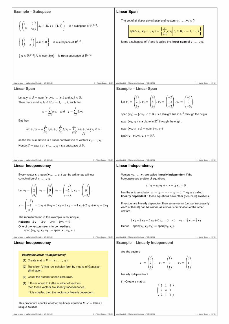
(a11 00 a22
)∣∣∣∣∣ aii ∈ R, i ∈ 1, 2
is a subspace of R2×2.
(a −bb a
)∣∣∣∣∣ a, b ∈ R
is a subspace of R2×2.
A ∈ R2×2
∣∣A is invertible
is not a subspace of R2×2.
Josef Leydold – Mathematical Methods – WS 2021/22 4 – Vector Space – 9 / 54
Linear Span
The set of all linear combinations of vectors v1, . . . , vk ∈ V
span(v1, v2, . . . , vk) =
k
∑i=1
civi
∣∣∣∣∣ ci ∈ R, i = 1, . . . , k
forms a subspace of V and is called the linear span of v1, . . . , vk.
Josef Leydold – Mathematical Methods – WS 2021/22 4 – Vector Space – 10 / 54
Linear Span
Let x, y ∈ S = span(v1, v2, . . . , vk) and α, β ∈ R.
Then there exist ai, bi ∈ R, i = 1, . . . , k, such that
x =k
∑i=1
aivi and y =k
∑i=1
bivi .
But then
αx + βy = αk
∑i=1
aivi + βk
∑i=1
bivi =k
∑i=1
(αai + βbi)︸ ︷︷ ︸∈R
vi ∈ S
as the last summation is a linear combination of vectors v1, . . . , vk.
Hence S = span(v1, v2, . . . , vk) is a subspace of V .
Josef Leydold – Mathematical Methods – WS 2021/22 4 – Vector Space – 11 / 54
Example – Linear Span
Let v1 =
123
, v2 =
456
, v3 =
−2−2−2
, v4 =
−10−3
.
span (v1) = c v1 : c ∈ R is a straight line in R3 through the origin.
span (v1, v2) is a plane in R3 through the origin.
span (v1, v2, v3) = span (v1, v2)
span(v1, v2, v3, v4) = R3.
Josef Leydold – Mathematical Methods – WS 2021/22 4 – Vector Space – 12 / 54
Linear Independency
Every vector x ∈ span(v1, . . . , vk) can be written as a linearcombination of v1, . . . , vk.
Let v1 =
123
, v2 =
456
, v3 =
−2−2−2
, v4 =
−10−3
.
x =
−3−43
= 1 v1 + 0 v2 + 3 v3− 2 v4 = −1 v1 + 2 v2 + 6 v3− 2 v4
The representation in this example is not unique!
Reason: 2 v1 − 2 v2 − 3 v3 + 0 v4 = 0One of the vectors seems to be needless:
span (v1, v2, v3, v4) = span (v1, v2, v4)
Josef Leydold – Mathematical Methods – WS 2021/22 4 – Vector Space – 13 / 54
Linear Independency
Vectors v1, . . . , vk are called linearly independent if thehomogeneous system of equations
c1 v1 + c2 v2 + · · ·+ ck vk = 0
has the unique solution c1 = c2 = · · · = ck = 0. They are calledlinearly dependent if these equations have other (non-zero) solutions.
If vectors are linearly dependent then some vector (but not necessarilyeach of these!) can be written as a linear combination of the othervectors.
2 v1 − 2 v2 − 3 v3 + 0 v4 = 0 ⇔ v3 = 23 v1 − 2
3 v2
Hence span(v1, v2, v3) = span(v1, v2).
Josef Leydold – Mathematical Methods – WS 2021/22 4 – Vector Space – 14 / 54
Linear Independency
Determine linear (in)dependency
(1) Create matrix V = (v1, . . . , vk).
(2) Transform V into row echelon form by means of Gaussianelimination.
(3) Count the number of non-zero rows.
(4) If this is equal to k (the number of vectors),then these vectors are linearly Independence.
If it is smaller, then the vectors or linearly dependent.
This procedure checks whether the linear equation V · c = 0 has aunique solution.
Josef Leydold – Mathematical Methods – WS 2021/22 4 – Vector Space – 15 / 54
Example – Linearly Independent
Are the vectors
v1 =
322
, v2 =
141
, v3 =
311
linearly independent?
(1) Create a matrix:
3 1 32 4 12 1 1
Josef Leydold – Mathematical Methods – WS 2021/22 4 – Vector Space – 16 / 54

Example – Linearly Independent
(2) Transform:
3 1 32 4 12 1 1
3 1 30 10 −30 1 −3
3 1 30 10 −30 0 −27
(3) We count 3 non-zero rows.
(4) The number of non-zero rows coincides withthe number of vectors (= 3).
Thus the three vectors v1, v2, and v3 are linearly independent.
Josef Leydold – Mathematical Methods – WS 2021/22 4 – Vector Space – 17 / 54
Example – Linearly Dependent
Are vectors v1 =
325
, v2 =
145
, v3 =
314
linearly independent?
(1) Create a matrix . . . (2) and transform:
3 1 32 4 15 5 4
3 1 30 10 −30 10 −3
3 1 30 10 −30 0 0
(3) We count 2 non-zero rows.
(4) The number of non-zero rows (= 2) is less than the number ofvectors (= 3).
Thus the three vectors v1, v2, and v3 are linearly dependent.
Josef Leydold – Mathematical Methods – WS 2021/22 4 – Vector Space – 18 / 54
Rank of a Matrix
The rank of matrix A is the maximal number of linearly independentcolumns.
We have: rank(AT) = rank(A)
The rank of an n× k matrix is at most min(n, k).
An n× n matrix is called regular, if it has full rank,i.e. if rank(A) = n.
Josef Leydold – Mathematical Methods – WS 2021/22 4 – Vector Space – 19 / 54
Rank of a Matrix
Computation of the rank:
(1) Transform matrix A into row echelon form by means ofGaussian elimination.
(2) Then rank(A) is given by the number of non-zero rows.
3 1 32 4 12 1 1
3 1 30 10 −30 0 −27
⇒ rank(A) = 3
3 1 32 4 15 5 4
3 1 30 10 −30 0 0
⇒ rank(A) = 2
Josef Leydold – Mathematical Methods – WS 2021/22 4 – Vector Space – 20 / 54
Invertible and Regular
An n× n matrix A is invertible, if and only if it is regular.
The following 3× 3 matrix
3 1 32 4 12 1 1
has full rank (3).
Thus it is regular and hence invertible.
The following 3× 3 matrix
3 1 32 4 15 5 4
has only rank 2.
Thus it is not regular and hence singular (i.e., not invertible).
Josef Leydold – Mathematical Methods – WS 2021/22 4 – Vector Space – 21 / 54
Basis
A set of vectors v1, . . . , vd spans (or generates) a vector space V , if
span(v1, . . . , vd) = V
This set is thus called a generating set for the vector space.
If these vectors are linearly independent, then this set is called a basisof the vector space.
The basis of a vector space is not uniquely determined!
However, the number of vectors in a basis is uniquely determined.It is called the dimension of the vector space.
dim(V) = d
Josef Leydold – Mathematical Methods – WS 2021/22 4 – Vector Space – 22 / 54
Characterizations of a Basis
There are several equivalent characterizations of a basis.
A basis B of vector space V is a
I linearly independent generating set of VI minimal generating set of V
(i.e., every proper subset of B does not span V )
I maximal linearly independent set(i.e., every proper superset of B is linearly dependent)
Josef Leydold – Mathematical Methods – WS 2021/22 4 – Vector Space – 23 / 54
Example – Basis
The so called canonical basis of the Rn consists of the n unit vectors:
B0 = e1, . . . , en ⊂ Rn
Thus we can conclude that
dim(Rn) = n
an that every basis of Rn consists of n (linearly independent) vectors.
Another basis of the R3:
322
,
141
,
311
Josef Leydold – Mathematical Methods – WS 2021/22 4 – Vector Space – 24 / 54
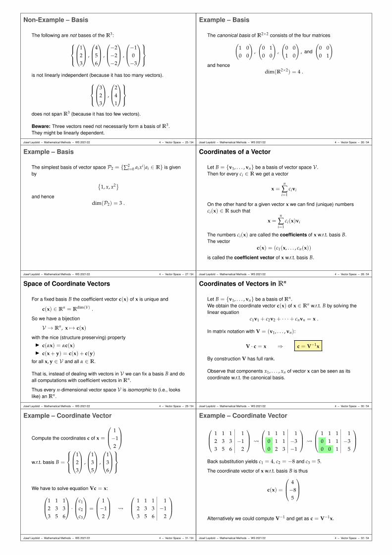
Non-Example – Basis
The following are not bases of the R3:
123
,
456
,
−2−2−2
,
−10−3
is not linearly independent (because it has too many vectors).
323
,
241
does not span R3 (because it has too few vectors).
Beware: Three vectors need not necessarily form a basis of R3.They might be linearly dependent.
Josef Leydold – Mathematical Methods – WS 2021/22 4 – Vector Space – 25 / 54
Example – Basis
The canonical basis of R2×2 consists of the four matrices(
1 00 0
),
(0 10 0
),
(0 01 0
), and
(0 00 1
)
and hencedim(R2×2) = 4 .
Josef Leydold – Mathematical Methods – WS 2021/22 4 – Vector Space – 26 / 54
Example – Basis
The simplest basis of vector space P2 = ∑2i=0 aixi|ai ∈ R is given
by
1, x, x2
and hencedim(P2) = 3 .
Josef Leydold – Mathematical Methods – WS 2021/22 4 – Vector Space – 27 / 54
Coordinates of a Vector
Let B = v1, . . . , vn be a basis of vector space V .Then for every ci ∈ R we get a vector
x =n
∑i=1
civi
On the other hand for a given vector x we can find (unique) numbersci(x) ∈ R such that
x =n
∑i=1
ci(x)vi
The numbers ci(x) are called the coefficients of x w.r.t. basis B.The vector
c(x) = (c1(x, . . . , cn(x))
is called the coefficient vector of x w.r.t. basis B.
Josef Leydold – Mathematical Methods – WS 2021/22 4 – Vector Space – 28 / 54
Space of Coordinate Vectors
For a fixed basis B the coefficient vector c(x) of x is unique and
c(x) ∈ Rn = Rdim(V) .
So we have a bijection
V → Rn, x 7→ c(x)
with the nice (structure preserving) propertyI c(αx) = αc(x)I c(x + y) = c(x) + c(y)
for all x, y ∈ V and all α ∈ R.
That is, instead of dealing with vectors in V we can fix a basis B and doall computations with coefficient vectors in Rn.
Thus every n-dimensional vector space V is isomorphic to (i.e., lookslike) an Rn.
Josef Leydold – Mathematical Methods – WS 2021/22 4 – Vector Space – 29 / 54
Coordinates of Vectors in Rn
Let B = v1, . . . , vn be a basis of Rn.We obtain the coordinate vector c(x) of x ∈ Rn w.r.t. B by solving thelinear equation
c1v1 + c2v2 + · · ·+ cnvn = x .
In matrix notation with V = (v1, . . . , vn):
V · c = x ⇒ c = V−1x
By construction V has full rank.
Observe that components x1, . . . , xn of vector x can be seen as itscoordinate w.r.t. the canonical basis.
Josef Leydold – Mathematical Methods – WS 2021/22 4 – Vector Space – 30 / 54
Example – Coordinate Vector
Compute the coordinates c of x =
1−12
w.r.t. basis B =
123
,
135
,
136
We have to solve equation Vc = x:
1 1 12 3 33 5 6
·
c1
c2
c3
=
1−12
1 1 1 12 3 3 −13 5 6 2
Josef Leydold – Mathematical Methods – WS 2021/22 4 – Vector Space – 31 / 54
Example – Coordinate Vector
1 1 1 12 3 3 −13 5 6 2
1 1 1 10 1 1 −30 2 3 −1
1 1 1 10 1 1 −30 0 1 5
Back substitution yields c1 = 4, c2 = −8 and c3 = 5.
The coordinate vector of x w.r.t. basis B is thus
c(x) =
4−85
Alternatively we could compute V−1 and get as c = V−1x.
Josef Leydold – Mathematical Methods – WS 2021/22 4 – Vector Space – 32 / 54

Change of Basis
Let c1 and c2 be the coordinate vectors of x ∈ V w.r.t. basesB1 = v1, v2, . . . , vn and B2 = w1, w2, . . . , wn, resp.
Consequently c2(x) = W−1x = W−1Vc1(x) .
Such a transformation of a coordinate vector w.r.t. one basis into that ofanother one is called a change of basis.
Matrix
U = W−1V
is called the transformation matrix for this change from basis B1 toB2.
Josef Leydold – Mathematical Methods – WS 2021/22 4 – Vector Space – 33 / 54
Example – Change of Basis
Let
B1 =
111
,
−211
,
356
and B2 =
123
,
135
,
136
two bases of R3.
Transformation matrix for the change of basis from B1 to B2:U = W−1 ·V.
W =
1 1 12 3 33 5 6
⇒ W−1 =
3 −1 0−3 3 −11 −2 1
V =
1 −2 31 1 51 1 6
Josef Leydold – Mathematical Methods – WS 2021/22 4 – Vector Space – 34 / 54
Example – Change of Basis
Transformation matrix for the change of basis from B1 to B2:
U = W−1 ·V =
3 −1 0−3 3 −11 −2 1
·
1 −2 31 1 51 1 6
=
2 −7 4−1 8 00 −3 −1
Let c1 = (3, 2, 1)T be the coordinate vector of x w.r.t. basis B1.Then the coordinate vector c2 w.r.t. basis B2 is given by
c2 = Uc1 =
2 −7 4−1 8 00 −3 −1
·
321
=
−413−7
Josef Leydold – Mathematical Methods – WS 2021/22 4 – Vector Space – 35 / 54
Linear Map
A map ϕ from vector space V intoW
ϕ : V → W , x 7→ y = ϕ(x)
is called linear, if for all x, y ∈ V and α ∈ R
(i) ϕ(x + y) = ϕ(x) + ϕ(y)(ii) ϕ(α x) = α ϕ(x)
We already have seen such a map: V → Rn, x 7→ c(x)
Josef Leydold – Mathematical Methods – WS 2021/22 4 – Vector Space – 36 / 54
Linear Map
Let A be an m× n matrix. Then mapϕ : Rn → Rm, x 7→ ϕA(x) = A · x is linear:
ϕA(x + y) = A · (x + y) = A · x + A · y = ϕA(x) + ϕA(y)
ϕA(α x) = A · (α x) = α (A · x) = α ϕA(x)
Vice versa every linear map ϕ : Rn → Rm can be represented by anappropriate m× n matrix Aϕ: ϕ(x) = Aϕ x.
Matrices represent all possible linear maps Rn → Rm.
More generally they represent linear maps between any vector spaceonce we have bases for these and do all computations with theircoordinate vectors.
In this sense, matrices “are” linear maps.
Josef Leydold – Mathematical Methods – WS 2021/22 4 – Vector Space – 37 / 54
Geometric Interpretation of Linear Maps
We have the following “elementary” maps:I dilation / shortening in some directionI projection into a subspaceI rotationI reflection at a subspace
These maps can be combined into more complex ones.
Josef Leydold – Mathematical Methods – WS 2021/22 4 – Vector Space – 38 / 54
Dilation / Shortening
Map ϕ : x 7→(
2 00 1
2
)x
dilates the x-coordinate by factor 2 andshortens the y-coordinate by factor 1
2 .
ϕ
Josef Leydold – Mathematical Methods – WS 2021/22 4 – Vector Space – 39 / 54
Projection
Map ϕ : x 7→(
12
12
12
12
)x
projects a point x orthogonally into the subspace generated by vector(1, 1)T, i.e., span
((1, 1)T
).
ϕ
Josef Leydold – Mathematical Methods – WS 2021/22 4 – Vector Space – 40 / 54

Rotation
Map ϕ : x 7→( √
22
√2
2−√
22
√2
2
)x
rotates a point x clock-wise by 45° around the origin.
ϕ
Josef Leydold – Mathematical Methods – WS 2021/22 4 – Vector Space – 41 / 54
Reflection
Map ϕ : x 7→(−1 00 1
)x
reflects a point x at the y-axis.
ϕ
Josef Leydold – Mathematical Methods – WS 2021/22 4 – Vector Space – 42 / 54
Image and Kernel
Let ϕ : Rn → Rm, x 7→ ϕ(x) = A · x be a linear map.
The image of ϕ is a subspace of Rm.
Im(ϕ) = ϕ(v) : v ∈ Rn ⊆ Rm
The kernel (or null space) of ϕ is a subspace of Rn.
Ker(ϕ) = v ∈ Rn : ϕ(v) = 0 ⊆ Rn
The kernel is the preimage of 0.
Image Im(A) and kernel Ker(A) of a matrix A are the respectiveimage and kernel of the corresponding linear map.
Josef Leydold – Mathematical Methods – WS 2021/22 4 – Vector Space – 43 / 54
Generating Set of the Image
Let A = (a1, . . . , an), x ∈ Rn an arbitrary vector, and ϕ(x) = Ax.
We can write x as a linear combination of the canonical basis:
x =n
∑i=1
xi ei
Recall that Aei = ai.So we can write ϕ(x) as a linear combination of the columns of A:
ϕ(x) = A · x = A ·n
∑i=1
xi ei =n
∑i=1
xi Aei =n
∑i=1
xi ai
That is, the columns ai of A span (generate) Im(ϕ).
Josef Leydold – Mathematical Methods – WS 2021/22 4 – Vector Space – 44 / 54
Basis of the Kernel
Let A = (a1, . . . , an) and ϕ(x) = Ax.
If y, z ∈ Ker(ϕ) and α, β ∈ R, then
ϕ(αy + βz) = αϕ(y) + βϕ(z) = α0 + β0 = 0
Thus Ker(ϕ) is closed under linear combination,i.e., Ker(ϕ) is a subspace.
We obtain a basis of Ker(ϕ) by solving the homogeneous linearequation A · x = 0 by means of Gaussian elimination.
Josef Leydold – Mathematical Methods – WS 2021/22 4 – Vector Space – 45 / 54
Dimension of Image and Kernel
Rank-nullity theorem:
dimV = dim Im(ϕ) + dim Ker(ϕ)
Josef Leydold – Mathematical Methods – WS 2021/22 4 – Vector Space – 46 / 54
Example – Dimension of Image and Kern
Map ϕ : R2 → R2, x 7→(
1 00 0
)x
projects a point x orthogonally onto the x axis.
Ker(ϕ)ϕ
Im(ϕ)
dim R2 = 2, dim Ker(ϕ) = 1 dim Im(ϕ) = 1
Josef Leydold – Mathematical Methods – WS 2021/22 4 – Vector Space – 47 / 54
Linear Map and Rank
The rank of matrix A = (a1, . . . , an) is (per definition) the dimension ofspan(a1, . . . , an).
Hence it is the dimension of the image of the corresponding linear map.
dim Im(ϕA) = rank(A)
The dimension of the solution set L of a homogeneous linear equationA x = 0 is then the kernel of this map.
dimL = dim Ker(ϕA) = dim Rn − dim Im(ϕA) = n− rank(A)
Josef Leydold – Mathematical Methods – WS 2021/22 4 – Vector Space – 48 / 54

Matrix Multiplication
By multiplying two matrices A and B we obtain the matrix of acompound linear map:
(ϕA ϕB)(x) = ϕA(ϕB(x)) = A (B x) = (A · B) x
Rn RmRkB A
AB
x Bx ABx
This point of view implies:
rank(A · B) ≤ min rank(A), rank(B)
Josef Leydold – Mathematical Methods – WS 2021/22 4 – Vector Space – 49 / 54
Non-Commutative Matrix Multiplication
A =
(1 00 1
3
)represents a shortening of the y-coordinate.
B =
(0 1−1 0
)represents a clock-wise rotation about 90°.
A B
Josef Leydold – Mathematical Methods – WS 2021/22 4 – Vector Space – 50 / 54
Non-Commutative Matrix Multiplication
A B
BAx
B A
ABx
Josef Leydold – Mathematical Methods – WS 2021/22 4 – Vector Space – 51 / 54
Inverse Matrix
The inverse matrix A−1 of A exists if and only if map ϕA(x) = A x isone-to-one and onto, i.e., if and only if
ϕA(x) = x1 a1 + · · ·+ xn an = 0 ⇔ x = 0
i.e., if and only ifA is regular.
From this point of view implies (A · B)−1 = B−1 ·A−1
Rn RmRkB A
AB
x Bx ABxB−1A−1z A−1z z
B−1A−1
Josef Leydold – Mathematical Methods – WS 2021/22 4 – Vector Space – 52 / 54
Similar Matrices
The basis of a vector space and thus the coordinates of a vector are notuniquely determined. Matrix Aϕ of a linear map ϕ : Rn → Rn alsodepends on the chosen bases.Let A be the matrix w.r.t. basis B1.Which matrix represents linear map ϕ if we use basis B2 instead?
basis B1 U x A−→ A U x
Ux yU−1
basis B2 x C−→ U−1 A U x
and thus C x = U−1 A U x
Two n× n matrices A and C are called similar, if there exists a regularmatrix U such that
C = U−1 A U
Josef Leydold – Mathematical Methods – WS 2021/22 4 – Vector Space – 53 / 54
Summary
I vector space and subspaceI linear independency and rankI basis and dimensionI coordinate vectorI change of basisI linear mapI image and kernelI similar matrices
Josef Leydold – Mathematical Methods – WS 2021/22 4 – Vector Space – 54 / 54
Chapter 5
Determinant
Josef Leydold – Mathematical Methods – WS 2021/22 5 – Determinant – 1 / 29
What is a Determinant?
We want to “compute” whether n vectors in Rn are linearly dependentand measure “how far” they are from being linearly dependent, resp.
Idea:
Two vectors in R2 span a parallelogram:
vectors are linearly dependent ⇔ area is zero
We use the n-dimensional volume of the created parallelepiped for ourfunction that “measures” linear dependency.
Josef Leydold – Mathematical Methods – WS 2021/22 5 – Determinant – 2 / 29
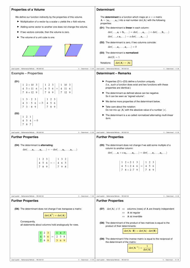
Properties of a Volume
We define our function indirectly by the properties of this volume.
I Multiplication of a vector by a scalar α yields the α-fold volume.
I Adding some vector to another one does not change the volume.
I If two vectors coincide, then the volume is zero.
I The volume of a unit cube is one.
Josef Leydold – Mathematical Methods – WS 2021/22 5 – Determinant – 3 / 29
Determinant
The determinant is a function which maps an n× n matrixA = (a1, . . . , an) into a real number det(A) with the followingproperties:
(D1) The determinant is linear in each column:
det(. . . , ai + bi, . . .) = det(. . . , ai, . . .) + det(. . . , bi, . . .)
det(. . . , α ai, . . .) = α det(. . . , ai, . . .)
(D2) The determinant is zero, if two columns coincide:
det(. . . , ai, . . . , ai, . . .) = 0
(D3) The determinant is normalized:
det(I) = 1
Notations: det(A) = |A|
Josef Leydold – Mathematical Methods – WS 2021/22 5 – Determinant – 4 / 29
Example – Properties
(D1) ∣∣∣∣∣∣∣
1 2 + 10 34 5 + 11 67 8 + 12 9
∣∣∣∣∣∣∣=
∣∣∣∣∣∣∣
1 2 34 5 67 8 9
∣∣∣∣∣∣∣+
∣∣∣∣∣∣∣
1 10 34 11 67 12 9
∣∣∣∣∣∣∣
∣∣∣∣∣∣∣
1 3 · 2 34 3 · 5 67 3 · 8 9
∣∣∣∣∣∣∣= 3 ·
∣∣∣∣∣∣∣
1 2 34 5 67 8 9
∣∣∣∣∣∣∣
(D2) ∣∣∣∣∣∣∣
1 2 14 5 47 8 7
∣∣∣∣∣∣∣= 0
Josef Leydold – Mathematical Methods – WS 2021/22 5 – Determinant – 5 / 29
Determinant – Remarks
I Properties (D1)–(D3) define a function uniquely.(I.e., such a function does exist and two functions with theseproperties are identical.)
I The determinant as defined above can be negative.So it can be seen as “signed volume”.
I We derive more properties of the determinant below.
I Take care about the notation:Do not mix up |A| with the absolute value of a number |x|.
I The determinant is a so called normalized alternating multi-linearform.
Josef Leydold – Mathematical Methods – WS 2021/22 5 – Determinant – 6 / 29
Further Properties
(D4) The determinant is alternating:
det(. . . , ai, . . . , ak, . . .) = −det(. . . , ak, . . . , ai, . . .)
∣∣∣∣∣∣∣
1 2 34 5 67 8 9
∣∣∣∣∣∣∣= −
∣∣∣∣∣∣∣
1 3 24 6 57 9 8
∣∣∣∣∣∣∣
Josef Leydold – Mathematical Methods – WS 2021/22 5 – Determinant – 7 / 29
Further Properties
(D5) The determinant does not change if we add some multiple of acolumn to another column:
det(. . . , ai + α ak, . . . , ak, . . .) = det(. . . , ai, . . . , ak, . . .)
∣∣∣∣∣∣∣
1 2 + 2 · 1 34 5 + 2 · 4 67 8 + 2 · 7 9
∣∣∣∣∣∣∣=
∣∣∣∣∣∣∣
1 2 34 5 67 8 9
∣∣∣∣∣∣∣
Josef Leydold – Mathematical Methods – WS 2021/22 5 – Determinant – 8 / 29
Further Properties
(D6) The determinant does not change if we transpose a matrix:
det(AT) = det(A)
Consequently,all statements about columns hold analogously for rows.
∣∣∣∣∣∣∣
1 2 34 5 67 8 9
∣∣∣∣∣∣∣=
∣∣∣∣∣∣∣
1 4 72 5 83 6 9
∣∣∣∣∣∣∣
Josef Leydold – Mathematical Methods – WS 2021/22 5 – Determinant – 9 / 29
Further Properties
(D7) det(A) 6= 0 ⇔ columns (rows) of A are linearly independent
⇔ A ist regular
⇔ A ist invertible
(D8) The determinant of the product of two matrices is equal to theproduct of their determinants:
det(A · B) = det(A) · det(B)
(D9) The determinant if the inverse matrix is equal to the reciprocal ofthe determinant of the matrix:
det(A−1) =1
det(A)
Josef Leydold – Mathematical Methods – WS 2021/22 5 – Determinant – 10 / 29
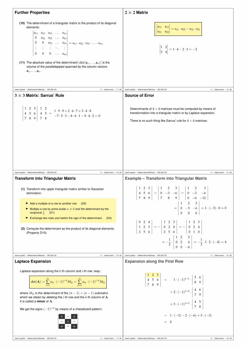
Further Properties
(10) The determinant of a triangular matrix is the product of its diagonalelements:∣∣∣∣∣∣∣∣∣∣∣∣∣
a11 a12 a13 . . . a1n
0 a22 a23 . . . a2n
0 0 a33 . . . a3n...
......
. . ....
0 0 0 . . . ann
∣∣∣∣∣∣∣∣∣∣∣∣∣
= a11 · a22 · a33 · . . . · ann
(11) The absolute value of the determinant |det(a1, . . . , an)| is thevolume of the parallelepiped spanned by the column vectorsa1, . . . , an.
Josef Leydold – Mathematical Methods – WS 2021/22 5 – Determinant – 11 / 29
2× 2 Matrix
∣∣∣∣∣a11 a12
a21 a22
∣∣∣∣∣ = a11 · a22 − a12 · a21
∣∣∣∣∣1 23 4
∣∣∣∣∣ = 1 · 4− 2 · 3 = −2
Josef Leydold – Mathematical Methods – WS 2021/22 5 – Determinant – 12 / 29
3× 3 Matrix: Sarrus’ Rule
1 2 3 1 24 5 6 4 57 8 9 7 8
=1 · 5 · 9 + 2 · 6 · 7 + 3 · 4 · 8−7 · 5 · 3− 8 · 6 · 1− 9 · 4 · 2 = 0
Josef Leydold – Mathematical Methods – WS 2021/22 5 – Determinant – 13 / 29
Source of Error
Determinants of 4× 4 matrices must be computed by means oftransformation into a triangular matrix or by Laplace expansion.
There is no such thing like Sarrus’ rule for 4× 4 matrices.
Josef Leydold – Mathematical Methods – WS 2021/22 5 – Determinant – 14 / 29
Transform into Triangular Matrix
(1) Transform into upper triangular matrix similar to Gaussianelimination.
I Add a multiple of a row to another row. (D5)
I Multiply a row by some scalar α 6= 0 and the determinant by thereciprocal 1
α . (D1)
I Exchange two rows and switch the sign of the determinant. (D4)
(2) Compute the determinant as the product of its diagonal elements.(Property D10)
Josef Leydold – Mathematical Methods – WS 2021/22 5 – Determinant – 15 / 29
Example – Transform into Triangular Matrix
∣∣∣∣∣∣∣
1 2 34 5 67 8 9
∣∣∣∣∣∣∣=
∣∣∣∣∣∣∣
1 2 30 −3 −67 8 9
∣∣∣∣∣∣∣=
∣∣∣∣∣∣∣
1 2 30 −3 −60 −6 −12
∣∣∣∣∣∣∣
=
∣∣∣∣∣∣∣
1 2 30 −3 −60 0 0
∣∣∣∣∣∣∣= 1 · (−3) · 0 = 0
∣∣∣∣∣∣∣
0 2 41 2 32 5 6
∣∣∣∣∣∣∣= −
∣∣∣∣∣∣∣
1 2 30 2 42 5 6
∣∣∣∣∣∣∣= −
∣∣∣∣∣∣∣
1 2 30 2 40 1 0
∣∣∣∣∣∣∣
= −12·
∣∣∣∣∣∣∣
1 2 30 2 40 0 −4
∣∣∣∣∣∣∣= −1
2· 1 · 2 · (−4) = 4
Josef Leydold – Mathematical Methods – WS 2021/22 5 – Determinant – 16 / 29
Laplace Expansion
Laplace expansion along the k-th column and i-th row, resp.:
det(A) =n
∑i=1
aik · (−1)i+k Mik =n
∑k=1
aik · (−1)i+k Mik
where Mik is the determinant of the (n− 1)× (n− 1) submatrixwhich we obtain by deleting the i-th row and the k-th column of A.It is called a minor of A.
We get the signs (−1)i+k by means of a chessboard pattern:∣∣∣∣∣∣∣
+ − +
− + −+ − +
∣∣∣∣∣∣∣
Josef Leydold – Mathematical Methods – WS 2021/22 5 – Determinant – 17 / 29
Expansion along the First Row
∣∣∣∣∣∣∣
1 2 34 5 67 8 9
∣∣∣∣∣∣∣= 1 · (−1)1+1 ·
∣∣∣∣∣5 68 9
∣∣∣∣∣
+ 2 · (−1)1+2 ·∣∣∣∣∣
4 67 9
∣∣∣∣∣
+ 3 · (−1)1+3 ·∣∣∣∣∣
4 57 8
∣∣∣∣∣
= 1 · (−3)− 2 · (−6) + 3 · (−3)
= 0
Josef Leydold – Mathematical Methods – WS 2021/22 5 – Determinant – 18 / 29
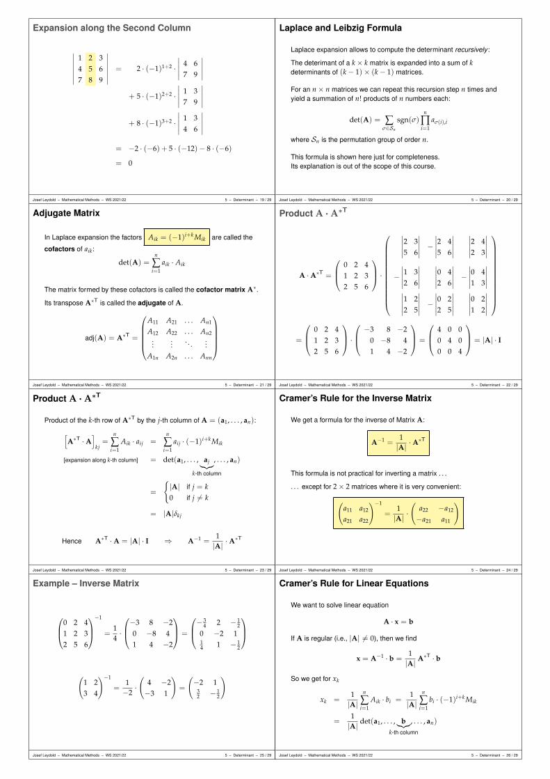
Expansion along the Second Column
∣∣∣∣∣∣∣
1 2 34 5 67 8 9
∣∣∣∣∣∣∣= 2 · (−1)1+2 ·
∣∣∣∣∣4 67 9
∣∣∣∣∣
+ 5 · (−1)2+2 ·∣∣∣∣∣
1 37 9
∣∣∣∣∣
+ 8 · (−1)3+2 ·∣∣∣∣∣
1 34 6
∣∣∣∣∣
= −2 · (−6) + 5 · (−12)− 8 · (−6)
= 0
Josef Leydold – Mathematical Methods – WS 2021/22 5 – Determinant – 19 / 29
Laplace and Leibzig Formula
Laplace expansion allows to compute the determinant recursively :
The deterimant of a k× k matrix is expanded into a sum of kdeterminants of (k− 1)× (k− 1) matrices.
For an n× n matrices we can repeat this recursion step n times andyield a summation of n! products of n numbers each:
det(A) = ∑σ∈Sn
sgn(σ)n
∏i=1
aσ(i),i
where Sn is the permutation group of order n.
This formula is shown here just for completeness.Its explanation is out of the scope of this course.
Josef Leydold – Mathematical Methods – WS 2021/22 5 – Determinant – 20 / 29
Adjugate Matrix
In Laplace expansion the factors Aik = (−1)i+k Mik are called the
cofactors of aik:
det(A) =n
∑i=1
aik · Aik
The matrix formed by these cofactors is called the cofactor matrix A∗.
Its transpose A∗T is called the adjugate of A.
adj(A) = A∗T =
A11 A21 . . . An1
A12 A22 . . . An2...
.... . .
...
A1n A2n . . . Ann
Josef Leydold – Mathematical Methods – WS 2021/22 5 – Determinant – 21 / 29
Product A ·A∗T
A ·A∗T =
0 2 41 2 32 5 6
·
∣∣∣∣∣2 35 6
∣∣∣∣∣ −∣∣∣∣∣2 45 6
∣∣∣∣∣
∣∣∣∣∣2 42 3
∣∣∣∣∣
−∣∣∣∣∣1 32 6
∣∣∣∣∣
∣∣∣∣∣0 42 6
∣∣∣∣∣ −∣∣∣∣∣0 41 3
∣∣∣∣∣∣∣∣∣∣1 22 5
∣∣∣∣∣ −∣∣∣∣∣0 22 5
∣∣∣∣∣
∣∣∣∣∣0 21 2
∣∣∣∣∣
=
0 2 41 2 32 5 6
·
−3 8 −2
0 −8 41 4 −2
=
4 0 00 4 00 0 4
= |A| · I
Josef Leydold – Mathematical Methods – WS 2021/22 5 – Determinant – 22 / 29
Product A ·A∗T
Product of the k-th row of A∗T by the j-th column of A = (a1, . . . , an):
[A∗T ·A
]kj=
n
∑i=1
Aik · aij =n
∑i=1
aij · (−1)i+k Mik
[expansion along k-th column] = det(a1, . . . , aj︸︷︷︸k-th column
, . . . , an)
=
|A| if j = k0 if j 6= k
= |A|δkj
Hence A∗T ·A = |A| · I ⇒ A−1 =1|A| ·A
∗T
Josef Leydold – Mathematical Methods – WS 2021/22 5 – Determinant – 23 / 29
Cramer’s Rule for the Inverse Matrix
We get a formula for the inverse of Matrix A:
A−1 =1|A| ·A
∗T
This formula is not practical for inverting a matrix . . .
. . . except for 2× 2 matrices where it is very convenient:
(a11 a12
a21 a22
)−1
=1|A| ·
(a22 −a12
−a21 a11
)
Josef Leydold – Mathematical Methods – WS 2021/22 5 – Determinant – 24 / 29
Example – Inverse Matrix
0 2 41 2 32 5 6
−1
=14·
−3 8 −20 −8 41 4 −2
=
− 3
4 2 − 12
0 −2 114 1 − 1
2
(1 23 4
)−1
=1−2·(
4 −2−3 1
)=
(−2 1
32 − 1
2
)
Josef Leydold – Mathematical Methods – WS 2021/22 5 – Determinant – 25 / 29
Cramer’s Rule for Linear Equations
We want to solve linear equation
A · x = b
If A is regular (i.e., |A| 6= 0), then we find
x = A−1 · b =1|A| A∗T · b
So we get for xk
xk =1|A|
n
∑i=1
Aik · bi =1|A|
n
∑i=1
bi · (−1)i+k Mik
=1|A| det(a1, . . . , b︸︷︷︸
k-th column
, . . . , an)
Josef Leydold – Mathematical Methods – WS 2021/22 5 – Determinant – 26 / 29
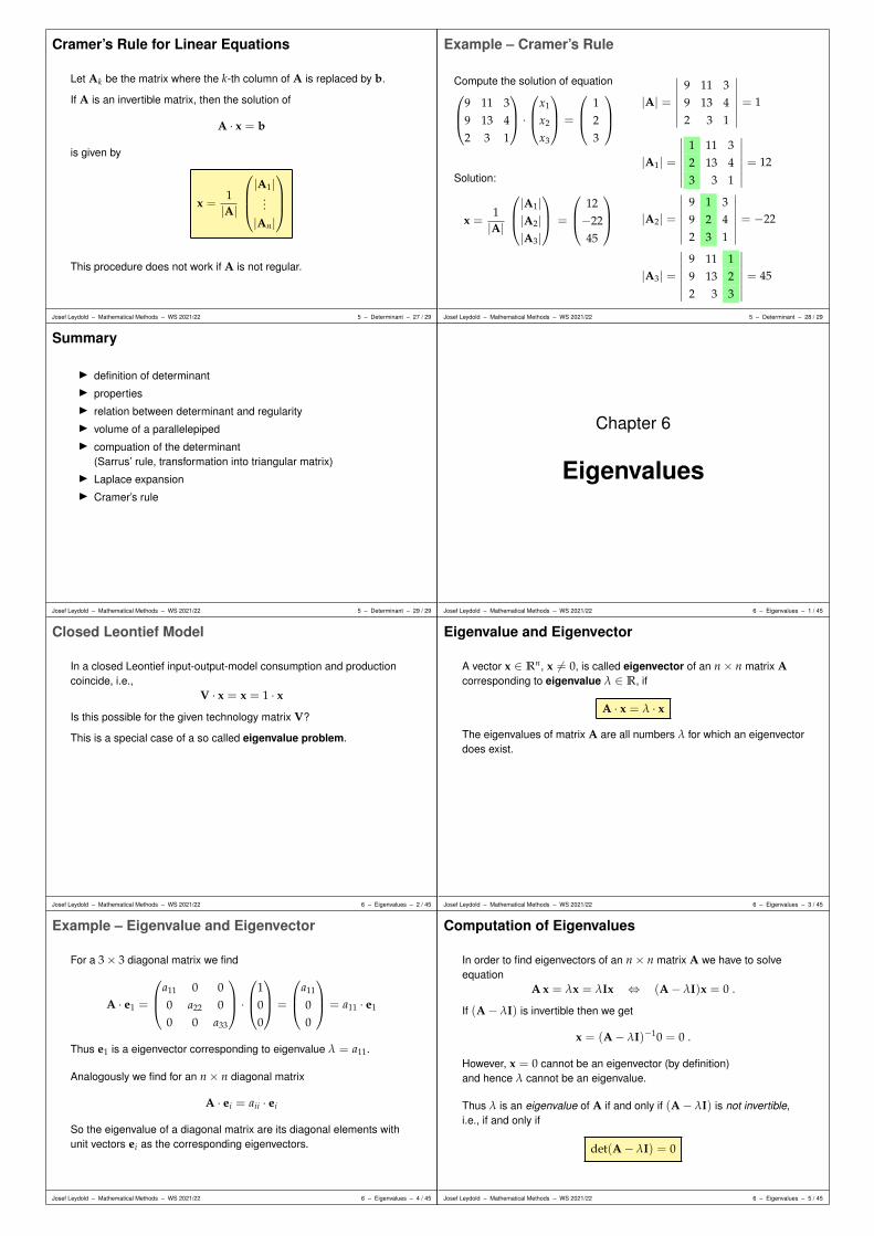
Cramer’s Rule for Linear Equations
Let Ak be the matrix where the k-th column of A is replaced by b.
If A is an invertible matrix, then the solution of
A · x = b
is given by
x =1|A|
|A1|...
|An|
This procedure does not work if A is not regular.
Josef Leydold – Mathematical Methods – WS 2021/22 5 – Determinant – 27 / 29
Example – Cramer’s Rule
Compute the solution of equation
9 11 39 13 42 3 1
·
x1
x2
x3
=
123
Solution:
x =1|A|
|A1||A2||A3|
=
12−2245
|A| =
∣∣∣∣∣∣∣
9 11 39 13 42 3 1
∣∣∣∣∣∣∣= 1
|A1| =
∣∣∣∣∣∣∣
1 11 32 13 43 3 1
∣∣∣∣∣∣∣= 12
|A2| =
∣∣∣∣∣∣∣
9 1 39 2 42 3 1
∣∣∣∣∣∣∣= −22
|A3| =
∣∣∣∣∣∣∣
9 11 19 13 22 3 3
∣∣∣∣∣∣∣= 45
Josef Leydold – Mathematical Methods – WS 2021/22 5 – Determinant – 28 / 29
Summary
I definition of determinantI propertiesI relation between determinant and regularityI volume of a parallelepipedI compuation of the determinant
(Sarrus’ rule, transformation into triangular matrix)I Laplace expansionI Cramer’s rule
Josef Leydold – Mathematical Methods – WS 2021/22 5 – Determinant – 29 / 29
Chapter 6
Eigenvalues
Josef Leydold – Mathematical Methods – WS 2021/22 6 – Eigenvalues – 1 / 45
Closed Leontief Model
In a closed Leontief input-output-model consumption and productioncoincide, i.e.,
V · x = x = 1 · xIs this possible for the given technology matrix V?
This is a special case of a so called eigenvalue problem.
Josef Leydold – Mathematical Methods – WS 2021/22 6 – Eigenvalues – 2 / 45
Eigenvalue and Eigenvector
A vector x ∈ Rn, x 6= 0, is called eigenvector of an n× n matrix Acorresponding to eigenvalue λ ∈ R, if
A · x = λ · x
The eigenvalues of matrix A are all numbers λ for which an eigenvectordoes exist.
Josef Leydold – Mathematical Methods – WS 2021/22 6 – Eigenvalues – 3 / 45
Example – Eigenvalue and Eigenvector
For a 3× 3 diagonal matrix we find
A · e1 =
a11 0 00 a22 00 0 a33
·
100
=
a11
00
= a11 · e1
Thus e1 is a eigenvector corresponding to eigenvalue λ = a11.
Analogously we find for an n× n diagonal matrix
A · ei = aii · ei
So the eigenvalue of a diagonal matrix are its diagonal elements withunit vectors ei as the corresponding eigenvectors.
Josef Leydold – Mathematical Methods – WS 2021/22 6 – Eigenvalues – 4 / 45
Computation of Eigenvalues
In order to find eigenvectors of an n× n matrix A we have to solveequation
A x = λx = λIx ⇔ (A− λI)x = 0 .
If (A− λI) is invertible then we get
x = (A− λI)−10 = 0 .
However, x = 0 cannot be an eigenvector (by definition)and hence λ cannot be an eigenvalue.
Thus λ is an eigenvalue of A if and only if (A− λI) is not invertible,i.e., if and only if
det(A− λI) = 0
Josef Leydold – Mathematical Methods – WS 2021/22 6 – Eigenvalues – 5 / 45
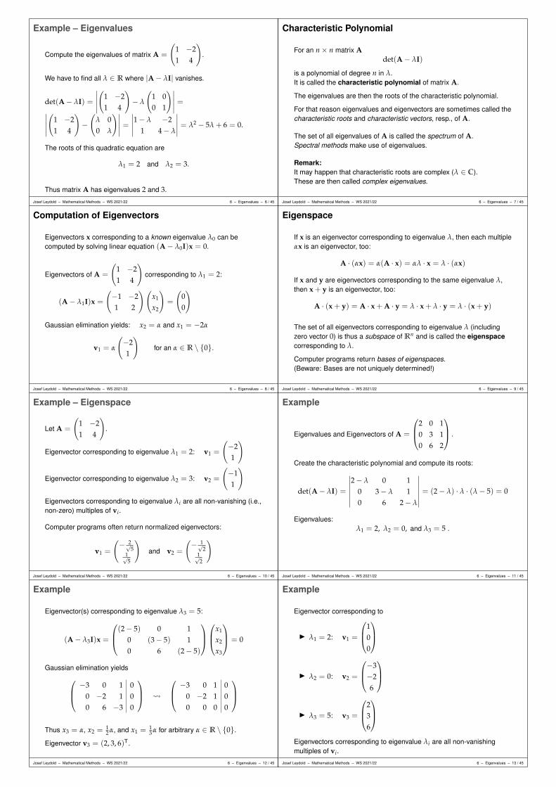
Example – Eigenvalues
Compute the eigenvalues of matrix A =
(1 −21 4
).
We have to find all λ ∈ R where |A− λI| vanishes.
det(A− λI) =
∣∣∣∣∣
(1 −21 4
)− λ
(1 00 1
)∣∣∣∣∣ =∣∣∣∣∣
(1 −21 4
)−(
λ 00 λ
)∣∣∣∣∣ =∣∣∣∣∣1− λ −2
1 4− λ
∣∣∣∣∣ = λ2 − 5λ + 6 = 0.
The roots of this quadratic equation are
λ1 = 2 and λ2 = 3.
Thus matrix A has eigenvalues 2 and 3.
Josef Leydold – Mathematical Methods – WS 2021/22 6 – Eigenvalues – 6 / 45
Characteristic Polynomial
For an n× n matrix Adet(A− λI)
is a polynomial of degree n in λ.It is called the characteristic polynomial of matrix A.
The eigenvalues are then the roots of the characteristic polynomial.
For that reason eigenvalues and eigenvectors are sometimes called thecharacteristic roots and characteristic vectors, resp., of A.
The set of all eigenvalues of A is called the spectrum of A.Spectral methods make use of eigenvalues.
Remark:It may happen that characteristic roots are complex (λ ∈ C).These are then called complex eigenvalues.
Josef Leydold – Mathematical Methods – WS 2021/22 6 – Eigenvalues – 7 / 45
Computation of Eigenvectors
Eigenvectors x corresponding to a known eigenvalue λ0 can becomputed by solving linear equation (A− λ0I)x = 0.
Eigenvectors of A =
(1 −21 4
)corresponding to λ1 = 2:
(A− λ1I)x =
(−1 −21 2
)(x1
x2
)=
(00
)
Gaussian elimination yields: x2 = α and x1 = −2α
v1 = α
(−21
)for an α ∈ R \ 0.
Josef Leydold – Mathematical Methods – WS 2021/22 6 – Eigenvalues – 8 / 45
Eigenspace
If x is an eigenvector corresponding to eigenvalue λ, then each multipleαx is an eigenvector, too:
A · (αx) = α(A · x) = αλ · x = λ · (αx)
If x and y are eigenvectors corresponding to the same eigenvalue λ,then x + y is an eigenvector, too:
A · (x + y) = A · x + A · y = λ · x + λ · y = λ · (x + y)
The set of all eigenvectors corresponding to eigenvalue λ (includingzero vector 0) is thus a subspace of Rn and is called the eigenspacecorresponding to λ.
Computer programs return bases of eigenspaces.(Beware: Bases are not uniquely determined!)
Josef Leydold – Mathematical Methods – WS 2021/22 6 – Eigenvalues – 9 / 45
Example – Eigenspace
Let A =
(1 −21 4
).
Eigenvector corresponding to eigenvalue λ1 = 2: v1 =
(−21
)
Eigenvector corresponding to eigenvalue λ2 = 3: v2 =
(−11
)
Eigenvectors corresponding to eigenvalue λi are all non-vanishing (i.e.,non-zero) multiples of vi.
Computer programs often return normalized eigenvectors:
v1 =
(− 2√
51√5
)and v2 =
(− 1√
21√2
)
Josef Leydold – Mathematical Methods – WS 2021/22 6 – Eigenvalues – 10 / 45
Example
Eigenvalues and Eigenvectors of A =
2 0 10 3 10 6 2
.
Create the characteristic polynomial and compute its roots:
det(A− λI) =
∣∣∣∣∣∣∣
2− λ 0 10 3− λ 10 6 2− λ
∣∣∣∣∣∣∣= (2− λ) · λ · (λ− 5) = 0
Eigenvalues:λ1 = 2, λ2 = 0, and λ3 = 5 .
Josef Leydold – Mathematical Methods – WS 2021/22 6 – Eigenvalues – 11 / 45
Example
Eigenvector(s) corresponding to eigenvalue λ3 = 5:
(A− λ3I)x =
(2− 5) 0 1
0 (3− 5) 10 6 (2− 5)
x1
x2
x3
= 0
Gaussian elimination yields
−3 0 1 0
0 −2 1 00 6 −3 0
−3 0 1 0
0 −2 1 00 0 0 0
Thus x3 = α, x2 = 12 α, and x1 = 1
3 α for arbitrary α ∈ R \ 0.Eigenvector v3 = (2, 3, 6)T.
Josef Leydold – Mathematical Methods – WS 2021/22 6 – Eigenvalues – 12 / 45
Example
Eigenvector corresponding to
I λ1 = 2: v1 =
100
I λ2 = 0: v2 =
−3−26
I λ3 = 5: v3 =
236
Eigenvectors corresponding to eigenvalue λi are all non-vanishingmultiples of vi.
Josef Leydold – Mathematical Methods – WS 2021/22 6 – Eigenvalues – 13 / 45
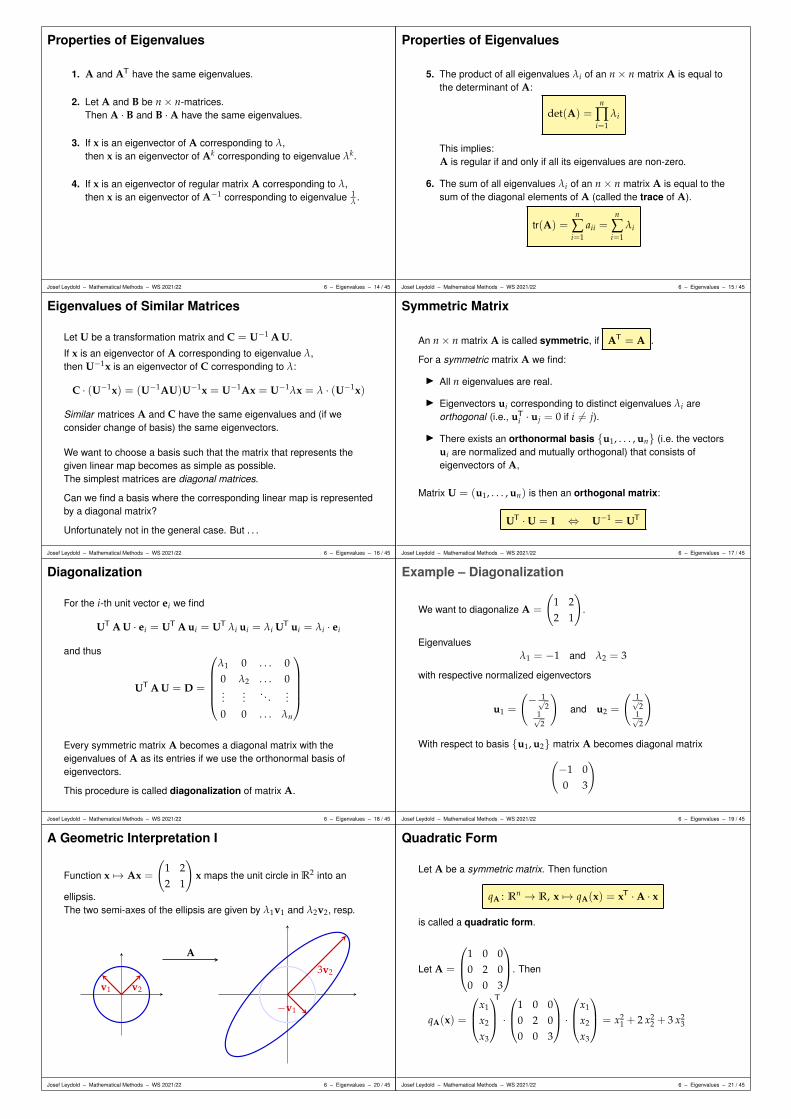
Properties of Eigenvalues
1. A and AT have the same eigenvalues.
2. Let A and B be n× n-matrices.Then A · B and B ·A have the same eigenvalues.
3. If x is an eigenvector of A corresponding to λ,then x is an eigenvector of Ak corresponding to eigenvalue λk.
4. If x is an eigenvector of regular matrix A corresponding to λ,then x is an eigenvector of A−1 corresponding to eigenvalue 1
λ .
Josef Leydold – Mathematical Methods – WS 2021/22 6 – Eigenvalues – 14 / 45
Properties of Eigenvalues
5. The product of all eigenvalues λi of an n× n matrix A is equal tothe determinant of A:
det(A) =n
∏i=1
λi
This implies:A is regular if and only if all its eigenvalues are non-zero.
6. The sum of all eigenvalues λi of an n× n matrix A is equal to thesum of the diagonal elements of A (called the trace of A).
tr(A) =n
∑i=1
aii =n
∑i=1
λi
Josef Leydold – Mathematical Methods – WS 2021/22 6 – Eigenvalues – 15 / 45
Eigenvalues of Similar Matrices
Let U be a transformation matrix and C = U−1 A U.
If x is an eigenvector of A corresponding to eigenvalue λ,then U−1x is an eigenvector of C corresponding to λ:
C · (U−1x) = (U−1AU)U−1x = U−1Ax = U−1λx = λ · (U−1x)
Similar matrices A and C have the same eigenvalues and (if weconsider change of basis) the same eigenvectors.
We want to choose a basis such that the matrix that represents thegiven linear map becomes as simple as possible.The simplest matrices are diagonal matrices.
Can we find a basis where the corresponding linear map is representedby a diagonal matrix?
Unfortunately not in the general case. But . . .
Josef Leydold – Mathematical Methods – WS 2021/22 6 – Eigenvalues – 16 / 45
Symmetric Matrix
An n× n matrix A is called symmetric, if AT = A .
For a symmetric matrix A we find:
I All n eigenvalues are real.
I Eigenvectors ui corresponding to distinct eigenvalues λi areorthogonal (i.e., uT
i · uj = 0 if i 6= j).
I There exists an orthonormal basis u1, . . . , un (i.e. the vectorsui are normalized and mutually orthogonal) that consists ofeigenvectors of A,
Matrix U = (u1, . . . , un) is then an orthogonal matrix:
UT ·U = I ⇔ U−1 = UT
Josef Leydold – Mathematical Methods – WS 2021/22 6 – Eigenvalues – 17 / 45
Diagonalization
For the i-th unit vector ei we find
UT A U · ei = UT A ui = UT λi ui = λi UT ui = λi · ei
and thus
UT A U = D =
λ1 0 . . . 00 λ2 . . . 0...
.... . .
...
0 0 . . . λn
Every symmetric matrix A becomes a diagonal matrix with theeigenvalues of A as its entries if we use the orthonormal basis ofeigenvectors.
This procedure is called diagonalization of matrix A.
Josef Leydold – Mathematical Methods – WS 2021/22 6 – Eigenvalues – 18 / 45
Example – Diagonalization
We want to diagonalize A =
(1 22 1
).
Eigenvaluesλ1 = −1 and λ2 = 3
with respective normalized eigenvectors
u1 =
(− 1√
21√2
)and u2 =
(1√2
1√2
)
With respect to basis u1, u2 matrix A becomes diagonal matrix(−1 00 3
)
Josef Leydold – Mathematical Methods – WS 2021/22 6 – Eigenvalues – 19 / 45
A Geometric Interpretation I
Function x 7→ Ax =
(1 22 1
)x maps the unit circle in R2 into an
ellipsis.The two semi-axes of the ellipsis are given by λ1v1 and λ2v2, resp.
v1 v2
A
−v1
3v2
Josef Leydold – Mathematical Methods – WS 2021/22 6 – Eigenvalues – 20 / 45
Quadratic Form
Let A be a symmetric matrix. Then function
qA : Rn → R, x 7→ qA(x) = xT ·A · x
is called a quadratic form.
Let A =
1 0 00 2 00 0 3
. Then
qA(x) =
x1
x2
x3
T
·
1 0 00 2 00 0 3
·
x1
x2
x3
= x2
1 + 2 x22 + 3 x2
3
Josef Leydold – Mathematical Methods – WS 2021/22 6 – Eigenvalues – 21 / 45
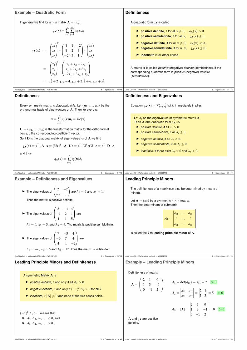
Example – Quadratic Form
In general we find for n× n matrix A = (aij):
qA(x) =n
∑i=1
n
∑j=1
aij xixj
qA(x) =
x1
x2
x3
T
·
1 1 −21 2 3−2 3 1
·
x1
x2
x3
=
x1
x2
x3
T
·
x1 + x2 − 2x3
x1 + 2x2 + 3x3
−2x1 + 3x2 + x3
= x21 + 2x1x2 − 4x1x3 + 2x2
2 + 6x2x3 + x23
Josef Leydold – Mathematical Methods – WS 2021/22 6 – Eigenvalues – 22 / 45
Definiteness
A quadratic form qA is called
I positive definite, if for all x 6= 0, qA(x) > 0.I positive semidefinite, if for all x, qA(x) ≥ 0.
I negative definite, if for all x 6= 0, qA(x) < 0.I negative semidefinite, if for all x, qA(x) ≤ 0.
I indefinite in all other cases.
A matrix A is called positive (negative) definite (semidefinite), if thecorresponding quadratic form is positive (negative) definite(semidefinite).
Josef Leydold – Mathematical Methods – WS 2021/22 6 – Eigenvalues – 23 / 45
Definiteness
Every symmetric matrix is diagonalizable. Let u1, . . . , un be theorthonormal basis of eigenvectors of A. Then for every x:
x =n
∑i=1
ci(x)ui = Uc(x)
U = (u1, . . . , un) is the transformation matrix for the orthonormalbasis, c the corresponding coefficient vector.
So if D is the diagonal matrix of eigenvalues λi of A we find
qA(x) = xT ·A · x = (Uc)T ·A ·Uc = cT ·UTAU · c = cT ·D · c
and thus
qA(x) =n
∑i=1
c2i (x)λi
Josef Leydold – Mathematical Methods – WS 2021/22 6 – Eigenvalues – 24 / 45
Definiteness and Eigenvalues
Equation qA(x) = ∑ni=1 c2
i (x)λi immediately implies:
Let λi be the eigenvalues of symmetric matrix A.Then A (the quadratic form qA) isI positive definite, if all λi > 0.I positive semidefinite, if all λi ≥ 0.
I negative definite, if all λi < 0.I negative semidefinite, if all λi ≤ 0.
I indefinite, if there exist λi > 0 and λj < 0.
Josef Leydold – Mathematical Methods – WS 2021/22 6 – Eigenvalues – 25 / 45
Example – Definiteness and Eigenvalues
I The eigenvalues of
(2 −2−2 5
)are λ1 = 6 and λ2 = 1.
Thus the matrix is positive definite.
I The eigenvalues of
5 −1 4−1 2 14 1 5
are
λ1 = 0, λ2 = 3, and λ3 = 9. The matrix is positive semidefinite.
I The eigenvalues of
7 −5 4−5 7 44 4 −2
are
λ1 = −6, λ2 = 6 and λ3 = 12. Thus the matrix is indefinite.
Josef Leydold – Mathematical Methods – WS 2021/22 6 – Eigenvalues – 26 / 45
Leading Principle Minors
The definiteness of a matrix can also be determined by means ofminors.
Let A = (aij) be a symmetric n× n matrix.Then the determinant of submatrix
Ak =
∣∣∣∣∣∣∣∣
a11 . . . a1k...
. . ....
ak1 . . . akk
∣∣∣∣∣∣∣∣
is called the k-th leading principle minor of A.
Josef Leydold – Mathematical Methods – WS 2021/22 6 – Eigenvalues – 27 / 45
Leading Principle Minors and Definiteness
A symmetric Matrix A is
I positive definite, if and only if all Ak > 0.
I negative definite, if and only if (−1)k Ak > 0 for all k.
I indefinite, if |A| 6= 0 and none of the two cases holds.
(−1)k Ak > 0 means thatI A1, A3, A5, . . . < 0, andI A2, A4, A6, . . . > 0.
Josef Leydold – Mathematical Methods – WS 2021/22 6 – Eigenvalues – 28 / 45
Example – Leading Principle Minors
Definiteness of matrix
A =
2 1 01 3 −10 −1 2
A and qA are positivedefinite.
A1 = det(a11) = a11 = 2 > 0
A2 =
∣∣∣∣∣a11 a12
a21 a22
∣∣∣∣∣ =∣∣∣∣∣2 11 3
∣∣∣∣∣ = 5 > 0
A3 = |A| =
∣∣∣∣∣∣∣
2 1 01 3 −10 −1 2
∣∣∣∣∣∣∣= 8 > 0
Josef Leydold – Mathematical Methods – WS 2021/22 6 – Eigenvalues – 29 / 45

Example – Leading Principle Minors
Definiteness of matrix
A =
1 1 −21 2 3−2 3 1
A and qA are indefinite.
A1 = det(a11) = a11 = 1 > 0
A2 =
∣∣∣∣∣a11 a12
a21 a22
∣∣∣∣∣ =∣∣∣∣∣1 11 2
∣∣∣∣∣ = 1 > 0
A3 = |A| =
∣∣∣∣∣∣∣
1 1 −21 2 3−2 3 1
∣∣∣∣∣∣∣= −28 < 0
Josef Leydold – Mathematical Methods – WS 2021/22 6 – Eigenvalues – 30 / 45
Principle Minors
Unfortunately the condition for semidefiniteness is more tedious.
Let A = (aij) be a symmetric n× n matrix.Then the determinant of submatrix
Ai1,...,ik =
∣∣∣∣∣∣∣∣
ai1,i1 . . . ai1,ik...
. . ....
aik ,i1 . . . aik ,ik
∣∣∣∣∣∣∣∣1 ≤ i1 < . . . < ik ≤ n.
is called a principle minor of order k of A.
Josef Leydold – Mathematical Methods – WS 2021/22 6 – Eigenvalues – 31 / 45
Principle Minors and Semidefiniteness
A symmetric matrix A is
I positive semidefinite, if and only if all Ai1,...,ik ≥ 0.
I negative semidefinite, if and only if (−1)k Ai1,...,ik ≥ 0 for all k.
I indefinite in all other cases.
(−1)k Ai1,...,ik ≥ 0 means thatI Ai1,...,ik ≥ 0, if k is even, andI Ai1,...,ik ≤ 0, if k is odd.
Josef Leydold – Mathematical Methods – WS 2021/22 6 – Eigenvalues – 32 / 45
Example – Principle Minors
Definiteness of matrix
A =
5 −1 4−1 2 14 1 5
The matrix ispositive semidefinite.
(But not positive definite!)
principle minors of order 1:A1 = 5 ≥ 0 A2 = 2 ≥ 0A3 = 5 ≥ 0
principle minors of order 2:
A1,2 =
∣∣∣∣∣5 −1−1 2
∣∣∣∣∣ = 9 ≥ 0
A1,3 =
∣∣∣∣∣5 44 5
∣∣∣∣∣ = 9 ≥ 0
A2,3 =
∣∣∣∣∣2 11 5
∣∣∣∣∣ = 9 ≥ 0
principle minors of order 3:A1,2,3 = |A| = 0 ≥ 0
Josef Leydold – Mathematical Methods – WS 2021/22 6 – Eigenvalues – 33 / 45
Example – Principle Minors
Definiteness of matrix
A =
−5 1 −41 −2 −1−4 −1 −5
The matrix isnegative semidefinite.
(But not negative definite!)
principle minors of order 1:A1 = −5 ≤ 0 A2 = −2 ≤ 0A3 = −5 ≤ 0
principle minors of order 2:
A1,2 =
∣∣∣∣∣−5 11 −2
∣∣∣∣∣ = 9 ≥ 0
A1,3 =
∣∣∣∣∣−5 −4−4 −5
∣∣∣∣∣ = 9 ≥ 0
A2,3 =
∣∣∣∣∣−2 −1−1 −5
∣∣∣∣∣ = 9 ≥ 0
principle minors of order 3:A1,2,3 = |A| = 0 ≤ 0
Josef Leydold – Mathematical Methods – WS 2021/22 6 – Eigenvalues – 34 / 45
Leading Principle Minors and Semidefiniteness
Obviously every positive definite matrix is also positive semidefinite(but not necessarily the other way round).
Matrix
A =
2 1 01 3 −10 −1 2
is positive definite as all leading principle minors are positive(see above).
Therefore A is also positive semidefinite.
In this case there is no need to compute the non-leading principleminors.
Josef Leydold – Mathematical Methods – WS 2021/22 6 – Eigenvalues – 35 / 45
Recipe for Semidefiniteness
Recipe for finding semidefiniteness of matrix A:
1. Compute all leading principle minors:I If the condition for positive definiteness holds, then
A is positive definite and thus positive semidefinite.I Else if the condition for negative definiteness holds, then
A is negative definite and thus negative semidefinite.I Else if det(A) 6= 0, then
A is indefinite.
2. Else also compute all non-leading principle minors:I If the condition for positive semidefiniteness holds, then
A is positive semidefinite.I Else if the condition for negative semidefiniteness holds, then
A is negative semidefinite.I Else
A is indefinite.
Josef Leydold – Mathematical Methods – WS 2021/22 6 – Eigenvalues – 36 / 45
Ellipse
Equationax2 + by2 = 1 , a, b > 0
describes an ellipse in canonical form.
1/√
b
1/√
a
The semi-axes have length 1√a and 1√
b, resp.
Josef Leydold – Mathematical Methods – WS 2021/22 6 – Eigenvalues – 37 / 45
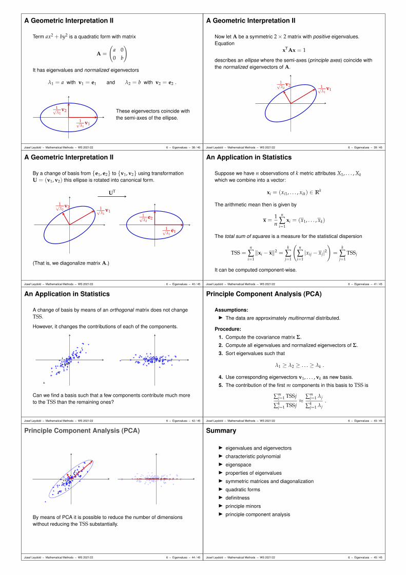
A Geometric Interpretation II
Term ax2 + by2 is a quadratic form with matrix
A =
(a 00 b
)
It has eigenvalues and normalized eigenvectors
λ1 = a with v1 = e1 and λ2 = b with v2 = e2 .
1√λ2
v2
1√λ1
v1
These eigenvectors coincide withthe semi-axes of the ellipse.
Josef Leydold – Mathematical Methods – WS 2021/22 6 – Eigenvalues – 38 / 45
A Geometric Interpretation II
Now let A be a symmetric 2× 2 matrix with positive eigenvalues.Equation
xTAx = 1
describes an ellipse where the semi-axes (principle axes) coincide withthe normalized eigenvectors of A.
1√λ2
v2 1√λ1
v1
Josef Leydold – Mathematical Methods – WS 2021/22 6 – Eigenvalues – 39 / 45
A Geometric Interpretation II
By a change of basis from e1, e2 to v1, v2 using transformationU = (v1, v2) this ellipse is rotated into canonical form.
1√λ2
v2 1√λ1
v1
UT
1√λ2
e2
1√λ1
e1
(That is, we diagonalize matrix A.)
Josef Leydold – Mathematical Methods – WS 2021/22 6 – Eigenvalues – 40 / 45
An Application in Statistics
Suppose we have n observations of k metric attributes X1, . . . , Xkwhich we combine into a vector:
xi = (xi1, . . . , xik) ∈ Rk
The arithmetic mean then is given by
x =1n
n
∑i=1
xi = (x1, . . . , xk)
The total sum of squares is a measure for the statistical dispersion
TSS =n
∑i=1‖xi − x‖2 =
k
∑j=1
(n
∑i=1|xij − xj|2
)=
k
∑j=1
TSSj
It can be computed component-wise.
Josef Leydold – Mathematical Methods – WS 2021/22 6 – Eigenvalues – 41 / 45
An Application in Statistics
A change of basis by means of an orthogonal matrix does not changeTSS.
However, it changes the contributions of each of the components.
Can we find a basis such that a few components contribute much moreto the TSS than the remaining ones?
Josef Leydold – Mathematical Methods – WS 2021/22 6 – Eigenvalues – 42 / 45
Principle Component Analysis (PCA)
Assumptions:I The data are approximately multinormal distributed.
Procedure:
1. Compute the covariance matrix Σ.
2. Compute all eigenvalues and normalized eigenvectors of Σ.
3. Sort eigenvalues such that
λ1 ≥ λ2 ≥ . . . ≥ λk .
4. Use corresponding eigenvectors v1, . . . , vk as new basis.
5. The contribution of the first m components in this basis to TSS is
∑mj=1 TSSj
∑kj=1 TSSj
≈ ∑mj=1 λj
∑kj=1 λj
.
Josef Leydold – Mathematical Methods – WS 2021/22 6 – Eigenvalues – 43 / 45
Principle Component Analysis (PCA)
By means of PCA it is possible to reduce the number of dimensionswithout reducing the TSS substantially.
Josef Leydold – Mathematical Methods – WS 2021/22 6 – Eigenvalues – 44 / 45
Summary
I eigenvalues and eigenvectorsI characteristic polynomialI eigenspaceI properties of eigenvaluesI symmetric matrices and diagonalizationI quadratic formsI definitnessI principle minorsI principle component analysis
Josef Leydold – Mathematical Methods – WS 2021/22 6 – Eigenvalues – 45 / 45
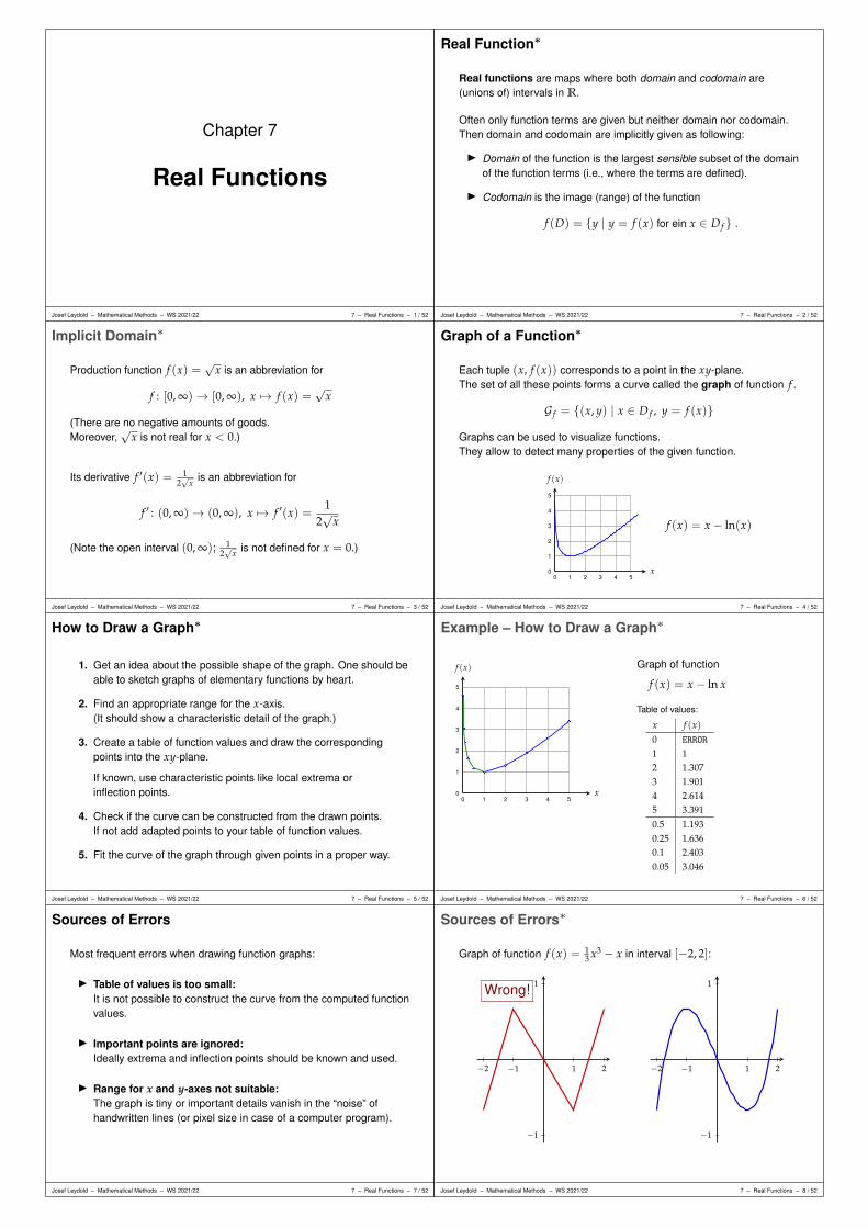
Chapter 7
Real Functions
Josef Leydold – Mathematical Methods – WS 2021/22 7 – Real Functions – 1 / 52
Real Function∗
Real functions are maps where both domain and codomain are(unions of) intervals in R.
Often only function terms are given but neither domain nor codomain.Then domain and codomain are implicitly given as following:
I Domain of the function is the largest sensible subset of the domainof the function terms (i.e., where the terms are defined).
I Codomain is the image (range) of the function
f (D) = y | y = f (x) for ein x ∈ D f .
Josef Leydold – Mathematical Methods – WS 2021/22 7 – Real Functions – 2 / 52
Implicit Domain∗
Production function f (x) =√
x is an abbreviation for
f : [0, ∞)→ [0, ∞), x 7→ f (x) =√
x
(There are no negative amounts of goods.Moreover,
√x is not real for x < 0.)
Its derivative f ′(x) = 12√
x is an abbreviation for
f ′ : (0, ∞)→ (0, ∞), x 7→ f ′(x) =1
2√
x
(Note the open interval (0, ∞); 12√
x is not defined for x = 0.)
Josef Leydold – Mathematical Methods – WS 2021/22 7 – Real Functions – 3 / 52
Graph of a Function∗
Each tuple (x, f (x)) corresponds to a point in the xy-plane.The set of all these points forms a curve called the graph of function f .
G f = (x, y) | x ∈ D f , y = f (x)
Graphs can be used to visualize functions.They allow to detect many properties of the given function.
x
f (x)
0 1 2 3 4 50
1
2
3
4
5
f (x) = x− ln(x)
Josef Leydold – Mathematical Methods – WS 2021/22 7 – Real Functions – 4 / 52
How to Draw a Graph∗
1. Get an idea about the possible shape of the graph. One should beable to sketch graphs of elementary functions by heart.
2. Find an appropriate range for the x-axis.(It should show a characteristic detail of the graph.)
3. Create a table of function values and draw the correspondingpoints into the xy-plane.
If known, use characteristic points like local extrema orinflection points.
4. Check if the curve can be constructed from the drawn points.If not add adapted points to your table of function values.
5. Fit the curve of the graph through given points in a proper way.
Josef Leydold – Mathematical Methods – WS 2021/22 7 – Real Functions – 5 / 52
Example – How to Draw a Graph∗
x
f (x)
0 1 2 3 4 50
1
2
3
4
5
Graph of function
f (x) = x− ln x
Table of values:
x f (x)0 ERROR1 12 1.3073 1.9014 2.6145 3.3910.5 1.1930.25 1.6360.1 2.4030.05 3.046
Josef Leydold – Mathematical Methods – WS 2021/22 7 – Real Functions – 6 / 52
Sources of Errors
Most frequent errors when drawing function graphs:
I Table of values is too small:It is not possible to construct the curve from the computed functionvalues.
I Important points are ignored:Ideally extrema and inflection points should be known and used.
I Range for x and y-axes not suitable:The graph is tiny or important details vanish in the “noise” ofhandwritten lines (or pixel size in case of a computer program).
Josef Leydold – Mathematical Methods – WS 2021/22 7 – Real Functions – 7 / 52
Sources of Errors∗
Graph of function f (x) = 13 x3 − x in interval [−2, 2]:
−2 −1 1 2
−1
1Wrong!
−2 −1 1 2
−1
1
Josef Leydold – Mathematical Methods – WS 2021/22 7 – Real Functions – 8 / 52
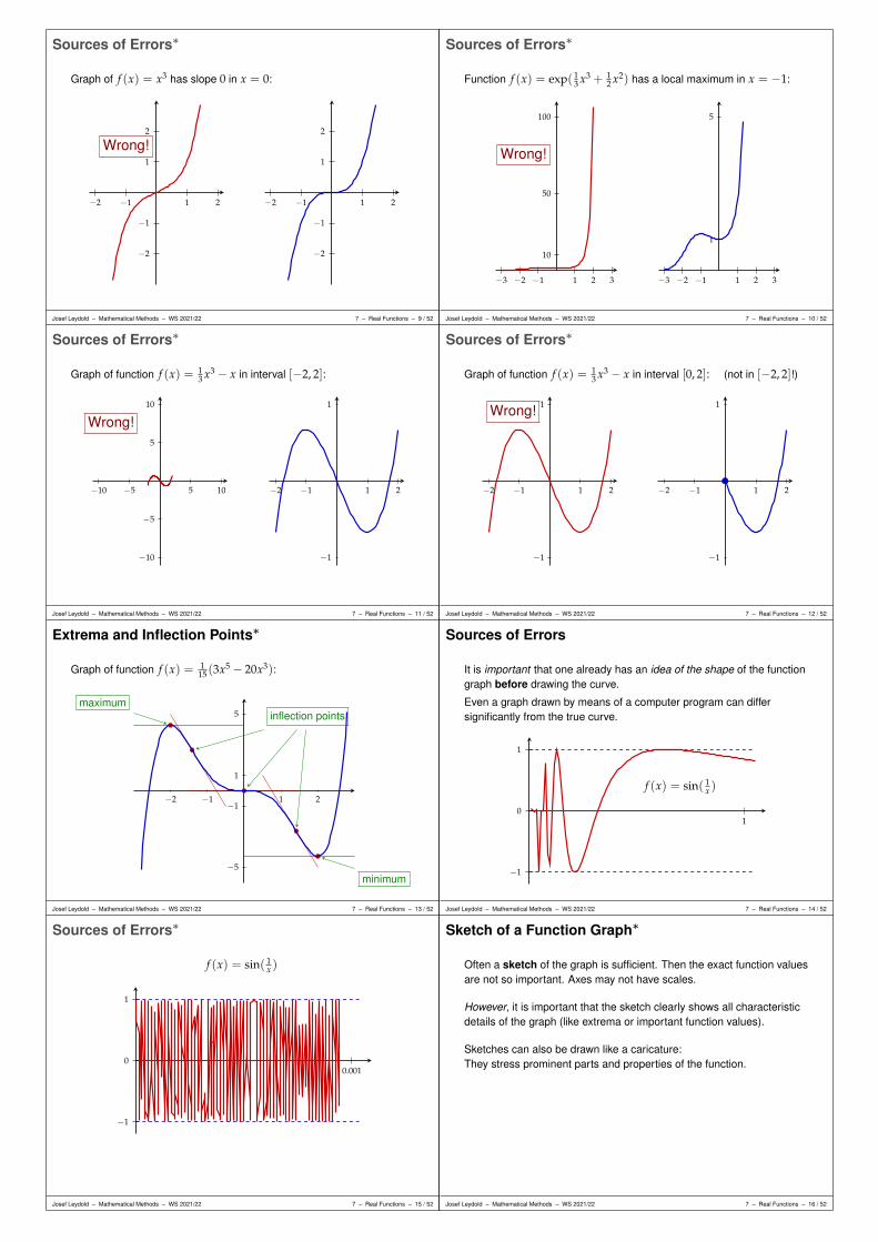
Sources of Errors∗
Graph of f (x) = x3 has slope 0 in x = 0:
−2 −1 1 2
−2
−1
1
2
Wrong!
−2 −1 1 2
−2
−1
1
2
Josef Leydold – Mathematical Methods – WS 2021/22 7 – Real Functions – 9 / 52
Sources of Errors∗
Function f (x) = exp( 13 x3 + 1
2 x2) has a local maximum in x = −1:
−3 −2 −1 1 2 3
10
50
100
Wrong!
−3 −2 −1 1 2 3
1
5
Josef Leydold – Mathematical Methods – WS 2021/22 7 – Real Functions – 10 / 52
Sources of Errors∗
Graph of function f (x) = 13 x3 − x in interval [−2, 2]:
−10 −5 5 10
−10
−5
5
10
Wrong!
−2 −1 1 2
−1
1
Josef Leydold – Mathematical Methods – WS 2021/22 7 – Real Functions – 11 / 52
Sources of Errors∗
Graph of function f (x) = 13 x3 − x in interval [0, 2]: (not in [−2, 2]!)
−2 −1 1 2
−1
1Wrong!
−2 −1 1 2
−1
1
Josef Leydold – Mathematical Methods – WS 2021/22 7 – Real Functions – 12 / 52
Extrema and Inflection Points∗
Graph of function f (x) = 115 (3x5 − 20x3):
−2 −1 1 2
−5
−1
1
5 inflection pointsmaximum
minimum
Josef Leydold – Mathematical Methods – WS 2021/22 7 – Real Functions – 13 / 52
Sources of Errors
It is important that one already has an idea of the shape of the functiongraph before drawing the curve.
Even a graph drawn by means of a computer program can differsignificantly from the true curve.
1
−1
0
1
f (x) = sin( 1x )
Josef Leydold – Mathematical Methods – WS 2021/22 7 – Real Functions – 14 / 52
Sources of Errors∗
f (x) = sin( 1x )
0.001
−1
0
1
Josef Leydold – Mathematical Methods – WS 2021/22 7 – Real Functions – 15 / 52
Sketch of a Function Graph∗
Often a sketch of the graph is sufficient. Then the exact function valuesare not so important. Axes may not have scales.
However, it is important that the sketch clearly shows all characteristicdetails of the graph (like extrema or important function values).
Sketches can also be drawn like a caricature:They stress prominent parts and properties of the function.
Josef Leydold – Mathematical Methods – WS 2021/22 7 – Real Functions – 16 / 52
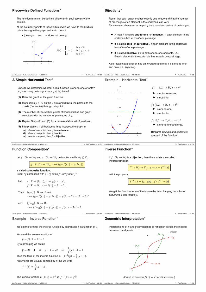
Piece-wise Defined Functions∗
The function term can be defined differently in subintervals of thedomain.
At the boundary points of these subintervals we have to mark whichpoints belong to the graph and which do not:
• (belongs) and (does not belong).
x
f (x)
−1 1 2
1
2
f (x) =
1, for x < 0,
1− x2
2 , for 0 ≤ x < 1,
x, for x ≥ 1.
Josef Leydold – Mathematical Methods – WS 2021/22 7 – Real Functions – 17 / 52
Bijectivity∗
Recall that each argument has exactly one image and that the numberof preimages of an element in the codomain can vary.Thus we can characterize maps by their possible number of preimages.
I A map f is called one-to-one (or injective), if each element in thecodomain has at most one preimage.
I It is called onto (or surjective), if each element in the codomainhas at least one preimage.
I It is called bijective, if it is both one-to-one and onto, i.e.,if each element in the codomain has exactly one preimage.
Also recall that a function has an inverse if and only if it is one-to-oneand onto (i.e., bijective).
Josef Leydold – Mathematical Methods – WS 2021/22 7 – Real Functions – 18 / 52
A Simple Horizontal Test∗
How can we determine whether a real function is one-to-one or onto?I.e., how many preimage may a y ∈W f have?
(1) Draw the graph of the given function.
(2) Mark some y ∈W on the y-axis and draw a line parallel to thex-axis (horizontal) through this point.
(3) The number of intersection points of horizontal line and graphcoincides with the number of preimages of y.
(4) Repeat Steps (2) and (3) for a representative set of y-values.
(5) Interpretation: If all horizontal lines intersect the graph in(a) at most one point, then f is one-to-one;(b) at least one point, then f is onto;(c) exactly one point, then f is bijective.
Josef Leydold – Mathematical Methods – WS 2021/22 7 – Real Functions – 19 / 52
Example – Horizontal Test∗
−1 1 2
1
2
3
4
5f : [−1, 2]→ R, x 7→ x2
I is not one-to-one;I is not onto.
f : [0, 2]→ R, x 7→ x2
I is one-to-one;I is not onto.
f : [0, 2]→ [0, 4], x 7→ x2
I is one-to-one and onto.
Beware! Domain and codomainare part of the function!
Josef Leydold – Mathematical Methods – WS 2021/22 7 – Real Functions – 20 / 52
Function Composition∗
Let f : D f →W f and g : Dg →Wg be functions with W f ⊆ Dg.
g f : D f →Wg, x 7→ (g f )(x) = g( f (x))
is called composite function.(read: “g composed with f ”, “g circle f ”, or “g after f ”)
Let g : R→ [0, ∞), x 7→ g(x) = x2,
f : R→ R, x 7→ f (x) = 3x− 2.
Then (g f ) : R→ [0, ∞),x 7→ (g f )(x) = g( f (x)) = g(3x− 2) = (3x− 2)2
and ( f g) : R→ R,x 7→ ( f g)(x) = f (g(x)) = f (x2) = 3x2 − 2
Josef Leydold – Mathematical Methods – WS 2021/22 7 – Real Functions – 21 / 52
Inverse Function∗
If f : D f →W f is a bijection, then there exists a so calledinverse function
f−1 : W f → D f , y 7→ x = f−1(y)
with the property
f−1 f = id and f f−1 = id
We get the function term of the inverse by interchanging the roles ofargument x and image y.
Josef Leydold – Mathematical Methods – WS 2021/22 7 – Real Functions – 22 / 52
Example – Inverse Function∗
We get the term for the inverse function by expressing x as function of y
We need the inverse function of
y = f (x) = 2x− 1
By rearranging we obtain
y = 2x− 1 ⇔ y + 1 = 2x ⇔ 12(y + 1) = x
Thus the term of the inverse function is f−1(y) = 12 (y + 1).
Arguments are usually denoted by x. So we write
f−1(x) =12(x + 1) .
The inverse function of f (x) = x3 is f−1(x) = 3√
x.
Josef Leydold – Mathematical Methods – WS 2021/22 7 – Real Functions – 23 / 52
Geometric Interpretation∗
Interchanging of x and y corresponds to reflection across the medianbetween x and y-axis.
medianf (x)
(x, y)
f−1(x)
(y, x)
(Graph of function f (x) = x3 and its inverse.)
Josef Leydold – Mathematical Methods – WS 2021/22 7 – Real Functions – 24 / 52
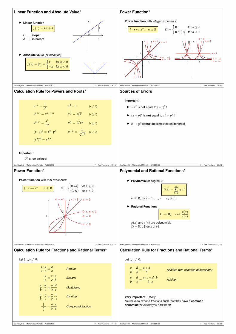
Linear Function and Absolute Value∗
I Linear function
f (x) = k x + d
k . . . sloped . . . intercept
d
k
1
I Absolute value (or modulus)
f (x) = |x| =
x for x ≥ 0−x for x < 0
Josef Leydold – Mathematical Methods – WS 2021/22 7 – Real Functions – 25 / 52
Power Function∗
Power function with integer exponents:
f : x 7→ xn, n ∈ Z D =
R for n ≥ 0R \ 0 for n < 0
−1
1
−1
1
n = 1n = 3
n = −1n = −3
−1 1
1n = 0
n = 2n = 4
n = −2n = −4
Josef Leydold – Mathematical Methods – WS 2021/22 7 – Real Functions – 26 / 52
Calculation Rule for Powers and Roots∗
x−n =1xn x0 = 1 (x 6= 0)
xn+m = xn · xm x1m = m
√x (x ≥ 0)
xn−m =xn
xm xnm = m
√xn (x ≥ 0)
(x · y)n = xn · yn x−nm =
1m√
xn(x ≥ 0)
(xn)m = xn·m
Important!
00 is not defined!
Josef Leydold – Mathematical Methods – WS 2021/22 7 – Real Functions – 27 / 52
Sources of Errors
Important!
I −x2 is not equal to (−x)2 !
I (x + y)n is not equal to xn + yn !
I xn + yn cannot be simplified (in general)!
Josef Leydold – Mathematical Methods – WS 2021/22 7 – Real Functions – 28 / 52
Power Function∗
Power function with real exponents:
f : x 7→ xα α ∈ R D =
[0, ∞) for α ≥ 0(0, ∞) for α < 0
1
1
α = 1α > 1α = ∞
0 < α < 1α = 0
α < 0
Josef Leydold – Mathematical Methods – WS 2021/22 7 – Real Functions – 29 / 52
Polynomial and Rational Functions∗
I Polynomial of degree n:
f (x) =n
∑k=0
ak xk
ai ∈ R, for i = 1, . . . , n, an 6= 0.
I Rational Function:
D → R, x 7→ p(x)q(x)
p(x) and q(x) are polynomialsD = R \ roots of q
Josef Leydold – Mathematical Methods – WS 2021/22 7 – Real Functions – 30 / 52
Calculation Rule for Fractions and Rational Terms∗
Let b, c, e 6= 0.
c · ac · b =
ab
Reduce
ab=
c · ac · b Expand
ab· d
c=
a · db · c Multiplying
ab
:ec=
ab· c
eDividing
abec
=a · cb · e Compound fraction
Josef Leydold – Mathematical Methods – WS 2021/22 7 – Real Functions – 31 / 52
Calculation Rule for Fractions and Rational Terms∗
Let b, c 6= 0.
ab+
db=
a + db
Addition with common denominator
ab+
dc=
a · c + d · bb · c Addition
Very important! Really!You have to expand fractions such that they have a commondenominator before you add them!
Josef Leydold – Mathematical Methods – WS 2021/22 7 – Real Functions – 32 / 52

Sources of Errors
Very Important! Really!
a + cb + c
is not equal toab
xa+
yb
is not equal tox + ya + b
ab + c
is not equal toab+
ac
x + 2y + 2
6= xy
12+
136= 1
5.
1x2 + y2 6=
1x2 +
1y2
Josef Leydold – Mathematical Methods – WS 2021/22 7 – Real Functions – 33 / 52
Exponential Function∗
I Exponential function:
R→ R+, x 7→ exp(x) = ex
e = 2, 7182818 . . . Euler’s number
I Generalized exponential function:
R→ R+, x 7→ ax a > 0
1
1
a
Josef Leydold – Mathematical Methods – WS 2021/22 7 – Real Functions – 34 / 52
Logarithm Function∗
I Logarithm:
Inverse function of exponential function.
R+ → R, x 7→ log(x) = ln(x)
I Generalized Logarithm to basis a:
R+ → R, x 7→ loga(x)
1
1
a
Josef Leydold – Mathematical Methods – WS 2021/22 7 – Real Functions – 35 / 52
Exponent and Logarithm∗
A number y is called the logarithm to basis a, if ay = x.The logarithm is the exponent of a number to basis a.We write
y = loga(x) ⇔ x = ay
Important logarithms:I natural logarithm ln(x) with basis e = 2.7182818 . . .
(sometimes called Euler’s number )I common logarithm lg(x) with basis 10
(sometimes called decadic or decimal logarithm)
Josef Leydold – Mathematical Methods – WS 2021/22 7 – Real Functions – 36 / 52
Calculations with Exponent and Logarithm∗
Conversation formula:
ax = ex ln(a) loga(x) =ln(x)ln(a)
Important:Often one can see log(x) without a basis.
In this case the basis is (should be) implicitly given by the context of thebook or article.
I In mathematics: natural logarithmfinancial mathematics, programs like R, Mathematica, Maxima, . . .
I In applied sciences: common logarithmeconomics, pocket calculator, Excel, . . .
Josef Leydold – Mathematical Methods – WS 2021/22 7 – Real Functions – 37 / 52
Calculation Rules for Exponent and Logarithm∗
ax+y = ax · ay loga(x · y) = loga(x) + loga(y)
ax−y = ax
ay loga(xy ) = loga(x)− loga(y)
(ax)y = ax·y loga(xβ) = β · loga(x)
(a · b)x = ax · bx
aloga(x) = x loga(ax) = x
a0 = 1 loga(1) = 0
loga(x) has (as real-valued function) domain x > 0!
Josef Leydold – Mathematical Methods – WS 2021/22 7 – Real Functions – 38 / 52
Trigonometric Functions∗
I Sine:
R→ [−1, 1], x 7→ sin(x)
I Cosine:
R→ [−1, 1], x 7→ cos(x)
1
−1
π2
π 3π2
2π
sin(x)
cos(x)
Beware!These functions use radian for their arguments, i.e., angles aremeasured by means of the length of arcs on the unit circle and not bydegrees. A right angle then corresponds to x = π/2.
Josef Leydold – Mathematical Methods – WS 2021/22 7 – Real Functions – 39 / 52
Sine and Cosine∗
α
1sin α
cos α
(cos α, sin α)
Josef Leydold – Mathematical Methods – WS 2021/22 7 – Real Functions – 40 / 52
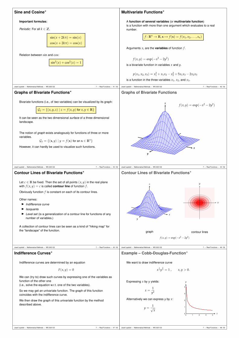
Sine and Cosine∗
Important formulas:
Periodic: For all k ∈ Z,
sin(x + 2kπ) = sin(x)
cos(x + 2kπ) = cos(x)
Relation between sin and cos:
sin2(x) + cos2(x) = 1
Josef Leydold – Mathematical Methods – WS 2021/22 7 – Real Functions – 41 / 52
Multivariate Functions∗
A function of several variables (or multivariate function)is a function with more than one argument which evaluates to a realnumber.
f : Rn → R, x 7→ f (x) = f (x1, x2, . . . , xn)
Arguments xi are the variables of function f .
f (x, y) = exp(−x2 − 2y2)
is a bivariate function in variables x and y.
p(x1, x2, x3) = x21 + x1x2 − x2
2 + 5x1x3 − 2x2x3
is a function in the three variables x1, x2, and x3.
Josef Leydold – Mathematical Methods – WS 2021/22 7 – Real Functions – 42 / 52
Graphs of Bivariate Functions∗
Bivariate functions (i.e., of two variables) can be visualized by its graph:
G f = (x, y, z) | z = f (x, y) for x, y ∈ R
It can be seen as the two dimensional surface of a three dimensionallandscape.
The notion of graph exists analogously for functions of three or morevariables.
G f = (x, y) | y = f (x) for an x ∈ RnHowever, it can hardly be used to visualize such functions.
Josef Leydold – Mathematical Methods – WS 2021/22 7 – Real Functions – 43 / 52
Graphs of Bivariate Functions
f (x, y) = exp(−x2 − 2y2)
x
y
z
x
y
z
Josef Leydold – Mathematical Methods – WS 2021/22 7 – Real Functions – 44 / 52
Contour Lines of Bivariate Functions∗
Let c ∈ R be fixed. Then the set of all points (x, y) in the real planewith f (x, y) = c is called contour line of function f .
Obviously function f is constant on each of its contour lines.
Other names:I Indifference curveI IsoquantsI Level set (is a generalization of a contour line for functions of any
number of variables.)
A collection of contour lines can be seen as a kind of “hiking map” forthe “landscape” of the function.
Josef Leydold – Mathematical Methods – WS 2021/22 7 – Real Functions – 45 / 52
Contour Lines of Bivariate Functions∗
x
y
z
x
y
graph contour lines
f (x, y) = exp(−x2 − 2y2)
Josef Leydold – Mathematical Methods – WS 2021/22 7 – Real Functions – 46 / 52
Indifference Curves∗
Indifference curves are determined by an equation
F(x, y) = 0
We can (try to) draw such curves by expressing one of the variables asfunction of the other one(i.e., solve the equation w.r.t. one of the two variables).
So we may get an univariate function. The graph of this functioncoincides with the indifference curve.
We then draw the graph of this univariate function by the methoddescribed above.
Josef Leydold – Mathematical Methods – WS 2021/22 7 – Real Functions – 47 / 52
Example – Cobb-Douglas-Function∗
We want to draw indifference curve
x13 y
23 = 1 , x, y > 0.
Expressing x by y yields:
x =1y2
Alternatively we can express y by x:
y =1√x
x
y
0 1 2 3 40
1
2
3
4
Josef Leydold – Mathematical Methods – WS 2021/22 7 – Real Functions – 48 / 52
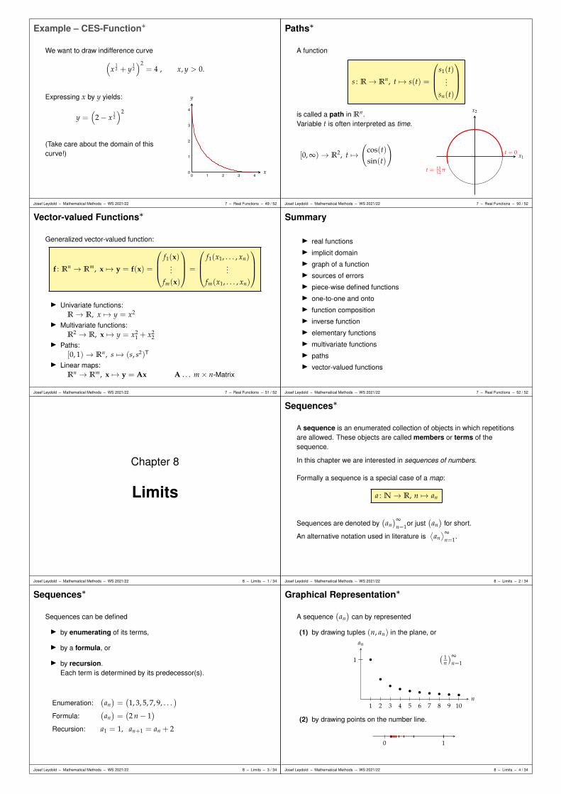
Example – CES-Function∗
We want to draw indifference curve(
x12 + y
12
)2= 4 , x, y > 0.
Expressing x by y yields:
y =(
2− x12
)2
(Take care about the domain of thiscurve!)
x
y
0 1 2 3 40
1
2
3
4
Josef Leydold – Mathematical Methods – WS 2021/22 7 – Real Functions – 49 / 52
Paths∗
A function
s : R→ Rn, t 7→ s(t) =
s1(t)...
sn(t)
is called a path in Rn.Variable t is often interpreted as time.
[0, ∞)→ R2, t 7→(
cos(t)sin(t)
)x1
x2
t = 0
t = 1312 π
Josef Leydold – Mathematical Methods – WS 2021/22 7 – Real Functions – 50 / 52
Vector-valued Functions∗
Generalized vector-valued function:
f : Rn → Rm, x 7→ y = f(x) =
f1(x)...
fm(x)
=
f1(x1, . . . , xn)...
fm(x1, . . . , xn)
I Univariate functions:R→ R, x 7→ y = x2
I Multivariate functions:R2 → R, x 7→ y = x2
1 + x22
I Paths:[0, 1)→ Rn, s 7→ (s, s2)T
I Linear maps:Rn → Rm, x 7→ y = Ax A . . . m× n-Matrix
Josef Leydold – Mathematical Methods – WS 2021/22 7 – Real Functions – 51 / 52
Summary
I real functionsI implicit domainI graph of a functionI sources of errorsI piece-wise defined functionsI one-to-one and ontoI function compositionI inverse functionI elementary functionsI multivariate functionsI pathsI vector-valued functions
Josef Leydold – Mathematical Methods – WS 2021/22 7 – Real Functions – 52 / 52
Chapter 8
Limits
Josef Leydold – Mathematical Methods – WS 2021/22 8 – Limits – 1 / 34
Sequences∗
A sequence is an enumerated collection of objects in which repetitionsare allowed. These objects are called members or terms of thesequence.
In this chapter we are interested in sequences of numbers.
Formally a sequence is a special case of a map:
a : N→ R, n 7→ an
Sequences are denoted by(an)∞
n=1or just(an)
for short.
An alternative notation used in literature is⟨
an⟩∞
n=1.
Josef Leydold – Mathematical Methods – WS 2021/22 8 – Limits – 2 / 34
Sequences∗
Sequences can be defined
I by enumerating of its terms,
I by a formula, or
I by recursion.Each term is determined by its predecessor(s).
Enumeration:(an)=(1, 3, 5, 7, 9, . . .
)
Formula:(an)=(2 n− 1
)
Recursion: a1 = 1, an+1 = an + 2
Josef Leydold – Mathematical Methods – WS 2021/22 8 – Limits – 3 / 34
Graphical Representation∗
A sequence(an)
can by represented
(1) by drawing tuples (n, an) in the plane, oran
n
1
1 2 3 4 5 6 7 8 9 10
•
•• • • • • • • •
( 1n
)∞n=1
(2) by drawing points on the number line.
0 1
Josef Leydold – Mathematical Methods – WS 2021/22 8 – Limits – 4 / 34
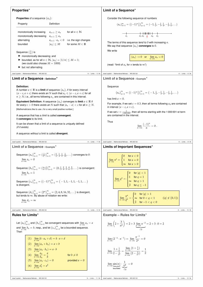
Properties∗
Properties of a sequence(an):
Property Definition
monotonically increasing an+1 ≥ an for all n ∈N
monotonically decreasing an+1 ≤ an
alternating an+1 · an < 0 i.e. the sign changes
bounded |an| ≤ M for some M ∈ R
Sequence( 1
n
)is
I monotonically decreasing; andI bounded, as for all n ∈N, |an| = |1/n| ≤ M = 1;
(we could also choose M = 1000)I but not alternating.
Josef Leydold – Mathematical Methods – WS 2021/22 8 – Limits – 5 / 34
Limit of a Sequence∗
Consider the following sequence of numbers
(an)∞n=1 =
((−1)n 1
n
)∞n=1 = (−1, 1
2 ,− 13 , 1
4 ,− 15 , 1
6 , . . .)
0a1 a2a3 a4a5
The terms of this sequence tend to 0 with increasing n.We say that sequence
(an)
converges to 0.
We write
(an)→ 0 or limn→∞
an = 0
(read: “limit of an for n tends to ∞”)
Josef Leydold – Mathematical Methods – WS 2021/22 8 – Limits – 6 / 34
Limit of a Sequence / Definition∗
Definition:A number a ∈ R is a limit of sequence
(an), if for every interval
(a− ε, a + ε) there exists an N such that an ∈ (a− ε, a + ε) for alln ≥ N; i.e., all terms following aN are contained in this interval.
Equivalent Definition: A sequence(an)
converges to limit a ∈ R iffor every ε > 0 there exists an N such that |an − a| < ε for all n ≥ N.
[Mathematicians like to use ε for a very small positive number.]
A sequence that has a limit is called convergent.It converges to its limit.
It can be shown that a limit of a sequence is uniquely defined(if it exists).
A sequence without a limit is called divergent.
Josef Leydold – Mathematical Methods – WS 2021/22 8 – Limits – 7 / 34
Limit of a Sequence / Example∗
Sequence
(an)∞
n=1 =((−1)n 1
n
)∞n=1 =
(− 1, 1
2 ,− 13 , 1
4 ,− 15 , 1
6 , . . .)
has limit a = 0.
For example, if we set ε = 0.3, then all terms following a4 are containedin interval (a− ε, a + ε).
If we set ε = 11 000 000 , then all terms starting with the 1 000 001-st term
are contained in the interval.
Thus
limn→∞
(−1)n
n= 0 .
Josef Leydold – Mathematical Methods – WS 2021/22 8 – Limits – 8 / 34
Limit of a Sequence / Example∗
Sequence(an)∞
n=1 =( 1
2n
)∞n=1 =
( 12 , 1
4 , 18 , 1
16 , . . .)
converges to 0:
limn→∞
an = 0
Sequence(bn)∞
n=1 =( n−1
n+1
)∞n=1 =
(0, 1
3 , 24 , 3
5 , 46 , 5
7 , . . .)
is convergent:
limn→∞
bn = 1
Sequence(cn)∞
n=1 =((−1)n)∞
n=1 =(− 1, 1,−1, 1,−1, 1, . . .
)
is divergent.
Sequence(dn)∞
n=1 =(2n)∞
n=1 =(2, 4, 8, 16, 32, . . .
)is divergent,
but tends to ∞. By abuse of notation we write:
limn→∞
dn = ∞
Josef Leydold – Mathematical Methods – WS 2021/22 8 – Limits – 9 / 34
Limits of Important Sequences∗
limn→∞
na =
0 for a < 01 for a = 0∞ for a > 0
limn→∞
qn =
0 for |q| < 11 for q = 1∞ for q > 1@ for q ≤ −1
limn→∞
na
qn =
0 for |q| > 1∞ for 0 < q < 1@ for −1 < q < 0
(|q| 6∈ 0, 1)
Josef Leydold – Mathematical Methods – WS 2021/22 8 – Limits – 10 / 34
Rules for Limits∗
Let(an)∞
n=1 and(bn)∞
n=1 be convergent sequences with limn→∞
an = a
and limn→∞
bn = b, resp., and let(cn)∞
n=1 be a bounded sequence.
Then
(1) limn→∞
(k · an + d) = k · a + d
(2) limn→∞
(an + bn) = a + b
(3) limn→∞
(an · bn) = a · b
(4) limn→∞
an
bn=
ab
for b 6= 0
(5) limn→∞
(an · cn) = 0 provided a = 0
(6) limn→∞
akn = ak
Josef Leydold – Mathematical Methods – WS 2021/22 8 – Limits – 11 / 34
Example – Rules for Limits∗
limn→∞
(2 +
3n2
)= 2 + 3 lim
n→∞n−2
︸ ︷︷ ︸=0
= 2 + 3 · 0 = 2
limn→∞
(2−n · n−1) = limn→∞
n−1
2n = 0
limn→∞
1 + 1n
2− 3n2
=limn→∞
(1 + 1
n
)
limn→∞
(2− 3
n2
) =12
limn→∞
sin(n)︸ ︷︷ ︸bounded
· 1n2︸︷︷︸→0
= 0
Josef Leydold – Mathematical Methods – WS 2021/22 8 – Limits – 12 / 34

Rules for Limits / Rational Terms∗
Important!When we apply these rules we have to take care that we never obtainexpressions of the form 0
0 , ∞∞ , or 0 ·∞.
These expressions are not defined!
limn→∞
3n2 + 1n2 − 1
=limn→∞
3n2 + 1
limn→∞
n2 − 1=
∞∞
(not defined)
Trick: Reduce the fraction by the largest power in its denominator.
limn→∞
3n2 + 1n2 − 1
= limn→∞
6n2
6n2 ·3 + n−2
1− n−2 =limn→∞
3 + n−2
limn→∞
1− n−2 =31= 3
Josef Leydold – Mathematical Methods – WS 2021/22 8 – Limits – 13 / 34
Euler’s Number∗
limn→∞
(1 +
1n
)n
= e = 2.7182818284590 . . .
This limit is very important in many applications including finance(continuous compounding).
limn→∞
(1 +
xn
)n= lim
n→∞
(1 +
1n/x
)n
= limm→∞
(1 +
1m
)mx (m =
nx
)
=
(lim
m→∞
(1 +
1m
)m)x
= ex
Josef Leydold – Mathematical Methods – WS 2021/22 8 – Limits – 14 / 34
Cauchy Sequence
How can we determine that a sequence converges if we have no clueabout the limit?
A sequence(an)∞
n=1 converges if and only if for every ε > 0 thereexists an N such that |an − am| < ε for all n, m ≥ N.
A sequence with such a property is called a Cauchy sequence.
Josef Leydold – Mathematical Methods – WS 2021/22 8 – Limits – 15 / 34
Series∗
The sum of the first n terms of sequence(ai)∞
i=1
sn =n
∑i=1
ai
is called the n-th partial sum of the sequence.
The sequence(sn)∞
n=1 of all partial sums is called the series of thesequence.
The series of sequence(ai)=(2 i− 1
)is
(sn)=
(n
∑i=1
(2 i− 1)
)=(1, 4, 9, 16, 25, . . .
)=(n2) .
Josef Leydold – Mathematical Methods – WS 2021/22 8 – Limits – 16 / 34
Limit of a Series∗
There are many cases where we have a summation overinfinitely many terms, ∑∞
i=1 ai.
However, then the usual rules for addition (in particular associativity andcommutativity) may not hold any more.Applying them in such cases would result in contradicitions.
Thus an “infinite sum” is defined as the limit of a series:
∞
∑i=1
ai = limn→∞
n
∑i=1
ai
For example,∞
∑k=1
12k = lim
n→∞
n
∑k=1
12k = lim
n→∞
12·( 1
2
)n − 112 − 1
= 1.
Josef Leydold – Mathematical Methods – WS 2021/22 8 – Limits – 17 / 34
Limit of a Function∗
What happens with the value of a function f , if the argument x tends tosome value x0 (which need not belong to the domain of f )?
Function
f (x) =x2 − 1x− 1
is not defined in x = 1.
By factorizing and reducing we getfunction
g(x) = x + 1 =
f (x), if x 6= 12, if x = 1
x
f (x)
−1 1 2
1
2
3
Josef Leydold – Mathematical Methods – WS 2021/22 8 – Limits – 18 / 34
Limit of a Function∗
Suppose we approach argument x0 = 1.
Then the value of function f (x) =x2 − 1x− 1
tends to 2.
We say:f (x) converges to 2 when x tends to 1
and write:
limx→1
x2 − 1x− 1
= 2
x
f (x)
−1 1 2
1
2
3
Josef Leydold – Mathematical Methods – WS 2021/22 8 – Limits – 19 / 34
Limit of a Function∗
Formal definition:If sequence
(f (xn))∞
n=1 of function values converges to number y0 forevery convergent sequence
(xn)∞
n=1 → x0 of arguments,then y0 is called the limit of f as x approaches x0.
We write
limx→x0
f (x) = y0 or f (x)→ y0 for x → x0
x0 need not belong to the domain of f .y0 need not belong to the codomain of f .
Josef Leydold – Mathematical Methods – WS 2021/22 8 – Limits – 20 / 34

Rules for Limits∗
Rules for limits of functions are analogous to rules for sequences.
Let limx→x0
f (x) = a and limx→x0
g(x) = b.
(1) limx→x0
(c · f (x) + d) = c · a + d
(2) limx→x0
( f (x) + g(x)) = a + b
(3) limx→x0
( f (x) · g(x)) = a · b
(4) limx→x0
f (x)g(x)
=ab
for b 6= 0
(6) limx→x0
( f (x))k = ak for k ∈N
Josef Leydold – Mathematical Methods – WS 2021/22 8 – Limits – 21 / 34
How to Find Limits?∗
The following recipe is suitable for “simple” functions:1. Draw the graph of the function.2. Mark x0 on the x-axis.3. Follow the graph with your pencil until we reach x0 starting from
right of x0.4. The y-coordinate of your pencil in this point is then the so called
right-handed limit of f as x approaches x0 (from above):lim
x→x+0f (x). (Other notations: lim
x↓x0f (x) or lim
xx0f (x))
5. Analogously we get the left-handed limit of f as x approaches x0(from below): lim
x→x−0f (x).
6. If both limits coincide, then the limit exists and we have
limx→x0
f (x) = limx→x−0
f (x) = limx→x+0
f (x)
Josef Leydold – Mathematical Methods – WS 2021/22 8 – Limits – 22 / 34
Example – How to Find Limits?∗
x
f (x)
−1 1 2
1
2
limx→1−
f (x)
limx→1+
f (x) f (x) =
1, for x < 01− x2
2 , for 0 ≤ x < 1x2 + 1, for x ≥ 1
0.5 = limx→1− f (x) 6= limx→1+ f (x) = 1.5i.e., the limit of f at x0 = 1 does not exist.
The limits at other points, however, do exist,e.g. lim
x→0f (x) = 1.
Josef Leydold – Mathematical Methods – WS 2021/22 8 – Limits – 23 / 34
Example – How to Find Limits?∗
x
f (x)
−1 1 2
1
2
f (x) =
1, for x < 00, for x = 01− x2
2 , for 0 < x < 1x2 + 1, for x ≥ 1
The only difference is to above is the function value at x0 = 0.Nevertheless, the limit does exist:
limx→0−
f (x) = 1 = limx→0+
f (x) ⇒ limx→0
f (x) = 1 .
Josef Leydold – Mathematical Methods – WS 2021/22 8 – Limits – 24 / 34
Unbounded Function∗
It may happen that f (x) tends to ∞ (or −∞) if x tends to x0.
We then write (by abuse of notation):
limx→x0
f (x) = ∞
x
f (x)
limx→0
1x2 = ∞
Josef Leydold – Mathematical Methods – WS 2021/22 8 – Limits – 25 / 34
Limit as x→ ∞∗
By abuse of language we can define the limit analogously for x0 = ∞
and x0 = −∞, resp.
Limitlimx→∞
f (x)
exists, if f (x) converges whenever x tends to infinity.
limx→∞
1x2 = 0 and lim
x→−∞
1x2 = 0
Josef Leydold – Mathematical Methods – WS 2021/22 8 – Limits – 26 / 34
Continuous Functions∗
We may observe that we can draw the graph of a function withoutremoving the pencil from paper. We call such functions continuous.
For some other functions we have to remove the pencil. At such pointsthe function has a jump discontinuity.
−2 −1 1 2
−1
1
−1 1 2
1
2
continuous jump discontinuity at x = 1
Josef Leydold – Mathematical Methods – WS 2021/22 8 – Limits – 27 / 34
Continuous Functions∗
Formal Definition:
Function f : D → R is called continuous at x0 ∈ D, if
1. limx→x0
f (x) exists, and
2. limx→x0
f (x) = f (x0) .
The function is called continuous if it is continuous at all points of itsdomain.
Note that continuity is a local property of a function.
Josef Leydold – Mathematical Methods – WS 2021/22 8 – Limits – 28 / 34
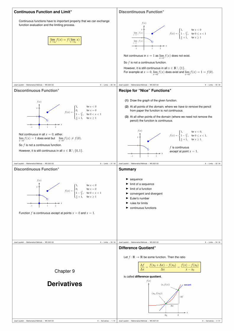
Continuous Function and Limit∗
Continuous functions have to important property that we can exchangefunction evaluation and the limiting process.
limx→x0
f (x) = f ( limx→x0
x)
Josef Leydold – Mathematical Methods – WS 2021/22 8 – Limits – 29 / 34
Discontinuous Function∗
x
f (x)
−1 1 2
1
2
limx→1−
f (x)
limx→1+
f (x) f (x) =
1, for x < 01− x2
2 , for 0 ≤ x < 1x2 + 1, for x ≥ 1
Not continuous in x = 1 as limx→1
f (x) does not exist.
So f is not a continuous function.
However, it is still continuous in all x ∈ R \ 1.For example at x = 0, lim
x→0f (x) does exist and lim
x→0f (x) = 1 = f (0).
Josef Leydold – Mathematical Methods – WS 2021/22 8 – Limits – 30 / 34
Discontinuous Function∗
x
f (x)
−1 1 2
1
2
f (x) =
1, for x < 00, for x = 01− x2
2 , for 0 < x < 1x2 + 1, for x ≥ 1
Not continuous in all x = 0, either.limx→0
f (x) = 1 does exist but limx→0
f (x) 6= f (0).
So f is not a continuous function.
However, it is still continuous in all x ∈ R \ 0, 1.
Josef Leydold – Mathematical Methods – WS 2021/22 8 – Limits – 31 / 34
Recipe for “Nice” Functions∗
(1) Draw the graph of the given function.
(2) At all points of the domain, where we have to remove the pencilfrom paper the function is not continuous.
(3) At all other points of the domain (where we need not remove thepencil) the function is continuous.
x
f (x)
−1 1 2
1
2f (x) =
1, for x < 0,
1− x2
2 , for 0 ≤ x < 1,x2 + 1, for x ≥ 1.
f is continuousexcept at point x = 1.
Josef Leydold – Mathematical Methods – WS 2021/22 8 – Limits – 32 / 34
Discontinuous Function∗
x
f (x)
−1 1 2
1
2
f (x) =
1, for x < 00, for x = 01− x2
2 , for 0 < x < 1x2 + 1, for x ≥ 1
Function f is continuous except at points x = 0 and x = 1.
Josef Leydold – Mathematical Methods – WS 2021/22 8 – Limits – 33 / 34
Summary
I sequenceI limit of a sequenceI limit of a functionI convergent and divergentI Euler’s numberI rules for limitsI continuous functions
Josef Leydold – Mathematical Methods – WS 2021/22 8 – Limits – 34 / 34
Chapter 9
Derivatives
Josef Leydold – Mathematical Methods – WS 2021/22 9 – Derivatives – 1 / 51
Difference Quotient∗
Let f : R→ R be some function. Then the ratio
∆ f∆x
=f (x0 + ∆x)− f (x0)
∆x=
f (x)− f (x0)
x− x0
is called difference quotient.
x
f (x)
x0 x
∆x
∆ f
secant
(x0, f (x0))
(x, f (x))
Josef Leydold – Mathematical Methods – WS 2021/22 9 – Derivatives – 2 / 51

Differential Quotient∗
If the limit
lim∆x→0
f (x0 + ∆x)− f (x0)
∆x= lim
x→x0
f (x)− f (x0)
x− x0
exists, then function f is called differentiable at x0. This limit is thencalled differential quotient or (first) derivative of function f at x0.
We write
f ′(x0) ord fdx
∣∣∣∣x=x0
Function f is called differentiable, if it is differentiable at each point of itsdomain.
Josef Leydold – Mathematical Methods – WS 2021/22 9 – Derivatives – 3 / 51
Slope of Tangent∗
I The differential quotient gives the slope of the tangent to the graphof function f (x) at x0.
x
f (x)
secants
x0
1
f ′(x0)
tangent
Josef Leydold – Mathematical Methods – WS 2021/22 9 – Derivatives – 4 / 51
Marginal Function∗
I Instantaneous change of function f .I “Marginal function” (as in marginal utility )
x
f (x)
x0
Josef Leydold – Mathematical Methods – WS 2021/22 9 – Derivatives – 5 / 51
Existence of Differential Quotient∗
Function f is differentiable at all points, where we can draw the tangent(with finite slope) uniquely to the graph.
Function f is not differentiable at all points where this is not possible.
In particular these areI jump discontinuitiesI “kinks” in the graph of the functionI vertical tangents
Josef Leydold – Mathematical Methods – WS 2021/22 9 – Derivatives – 6 / 51
Computation of the Differential Quotient∗
We can compute a differential quotient by determining the limit of thedifference quotient.
Let f (x) = x2. The we find for the first derivative
f ′(x0) = limh→0
(x0 + h)2 − x02
h
= limh→0
x02 + 2 x0 h + h2 − x0
2
h
= limh→0
2 x0 h + h2
h= lim
h→0(2 x0 + h)
= 2 x0
Josef Leydold – Mathematical Methods – WS 2021/22 9 – Derivatives – 7 / 51
Derivative of a Function∗
Function
f ′ : D → R, x 7→ f ′(x) =d fdx
∣∣∣∣x
is called the first derivative of function f .Its domain D is the set of all points where the differential quotient(i.e., the limit of the difference quotient) exists.
Josef Leydold – Mathematical Methods – WS 2021/22 9 – Derivatives – 8 / 51
Derivatives of Elementary Functions∗
f (x) f ′(x)
c 0
xα α · xα−1
ex ex
ln(x)1x
sin(x) cos(x)
cos(x) − sin(x)
Josef Leydold – Mathematical Methods – WS 2021/22 9 – Derivatives – 9 / 51
Computation Rules for Derivatives∗
I (c · f (x))′ = c · f ′(x)
I ( f (x) + g(x))′ = f ′(x) + g′(x) Summation rule
I ( f (x) · g(x))′ = f ′(x) · g(x) + f (x) · g′(x) Product rule
I ( f (g(x)))′ = f ′(g(x)) · g′(x) Chain rule
I
(f (x)g(x)
)′=
f ′(x) · g(x)− f (x) · g′(x)(g(x))2 Quotient rule
Josef Leydold – Mathematical Methods – WS 2021/22 9 – Derivatives – 10 / 51
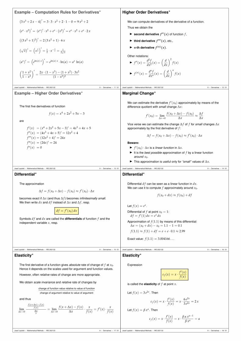
Example – Computation Rules for Derivatives∗
(3 x3 + 2 x− 4
)′= 3 · 3 · x2 + 2 · 1− 0 = 9 x2 + 2
(ex · x2)′ = (ex)′ · x2 + ex ·
(x2)′ = ex · x2 + ex · 2 x
((3 x2 + 1)2)′ = 2 (3 x2 + 1) · 6 x
(√x)′=(
x12
)′= 1
2 · x−12 = 1
2√
x
(ax)′ =(
eln(a)·x)′
= eln(a)·x · ln(a) = ax ln(a)
(1 + x2
1− x3
)′=
2x · (1− x3)− (1 + x2) · 3x2
(1− x3)2
Josef Leydold – Mathematical Methods – WS 2021/22 9 – Derivatives – 11 / 51
Higher Order Derivatives∗
We can compute derivatives of the derivative of a function.
Thus we obtain the
I second derivative f ′′(x) of function f ,
I third derivative f ′′′(x), etc.,
I n-th derivative f (n)(x).
Other notations:
I f ′′(x) =d2 fdx2 (x) =
(d
dx
)2
f (x)
I f (n)(x) =dn fdxn (x) =
(d
dx
)n
f (x)
Josef Leydold – Mathematical Methods – WS 2021/22 9 – Derivatives – 12 / 51
Example – Higher Order Derivatives∗
The first five derivatives of function
f (x) = x4 + 2x2 + 5x− 3
are
f ′(x) = (x4 + 2x2 + 5x− 3)′ = 4x3 + 4x + 5f ′′(x) = (4x3 + 4x + 5)′ = 12x2 + 4f ′′′(x) = (12x2 + 4)′ = 24xf ıv(x) = (24x)′ = 24f v(x) = 0
Josef Leydold – Mathematical Methods – WS 2021/22 9 – Derivatives – 13 / 51
Marginal Change∗
We can estimate the derivative f ′(x0) approximately by means of thedifference quotient with small change ∆x:
f ′(x0) = lim∆x→0
f (x0 + ∆x)− f (x0)
∆x≈ ∆ f
∆x
Vice verse we can estimate the change ∆ f of f for small changes ∆xapproximately by the first derivative of f :
∆ f = f (x0 + ∆x)− f (x0) ≈ f ′(x0) · ∆x
Beware:I f ′(x0) · ∆x is a linear function in ∆x.I It is the best possible approximation of f by a linear function
around x0.I This approximation is useful only for “small” values of ∆x.
Josef Leydold – Mathematical Methods – WS 2021/22 9 – Derivatives – 14 / 51
Differential∗
The approximation
∆ f = f (x0 + ∆x)− f (x0) ≈ f ′(x0) · ∆x
becomes exact if ∆x (and thus ∆ f ) becomes infinitesimally small.We then write dx and d f instead of ∆x and ∆ f , resp.
d f = f ′(x0) dx
Symbols d f and dx are called the differentials of function f and theindependent variable x, resp.
Josef Leydold – Mathematical Methods – WS 2021/22 9 – Derivatives – 15 / 51
Differential∗
Differential d f can be seen as a linear function in dx.We can use it to compute f approximately around x0.
f (x0 + dx) ≈ f (x0) + d f
Let f (x) = ex.
Differential of f at point x0 = 1:d f = f ′(1) dx = e1 dx
Approximation of f (1.1) by means of this differential:∆x = (x0 + dx)− x0 = 1.1− 1 = 0.1
f (1.1) ≈ f (1) + d f = e + e · 0.1 ≈ 2.99
Exact value: f (1.1) = 3.004166 . . .
Josef Leydold – Mathematical Methods – WS 2021/22 9 – Derivatives – 16 / 51
Elasticity∗
The first derivative of a function gives absolute rate of change of f at x0.Hence it depends on the scales used for argument and function values.
However, often relative rates of change are more appropriate.
We obtain scale invariance and relative rate of changes by
change of function value relative to value of function
change of argument relative to value of argument
and thus
lim∆x→0
f (x+∆x)− f (x)f (x)∆xx
= lim∆x→0
f (x + ∆x)− f (x)∆x
· xf (x)
= f ′(x) · xf (x)
Josef Leydold – Mathematical Methods – WS 2021/22 9 – Derivatives – 17 / 51
Elasticity∗
Expression
ε f (x) = x · f ′(x)f (x)
is called the elasticity of f at point x.
Let f (x) = 3 e2x. Then
ε f (x) = x · f ′(x)f (x)
= x · 6 e2x
3 e2x = 2 x
Let f (x) = β xα. Then
ε f (x) = x · f ′(x)f (x)
= x · β α xα−1
β xα= α
Josef Leydold – Mathematical Methods – WS 2021/22 9 – Derivatives – 18 / 51

Elasticity II∗
The relative rate of change of f can be expressed as
ln( f (x))′ =f ′(x)f (x)
What happens if we compute the derivative of ln( f (x)) w.r.t. ln(x)?
Let v = ln(x) ⇔ x = ev
Derivation by means of the chain rule yields:
d(ln( f (x)))d(ln(x))
=d(ln( f (ev)))
dv=
f ′(ev)
f (ev)ev =
f ′(x)f (x)
x = ε f (x)
ε f (x) =d(ln( f (x)))
d(ln(x))
Josef Leydold – Mathematical Methods – WS 2021/22 9 – Derivatives – 19 / 51
Elasticity II∗
We can use the chain rule formally in the following way:
LetI u = ln(y),I y = f (x),I x = ev ⇔ v = ln(x)
Then we find
d(ln f )d(ln x)
=dudv
=dudy· dy
dx· dx
dv=
1y· f ′(x) · ev =
f ′(x)f (x)
x
Josef Leydold – Mathematical Methods – WS 2021/22 9 – Derivatives – 20 / 51
Elastic Functions∗
A Function f is called
I elastic in x, if∣∣ ε f (x)
∣∣ > 1I 1-elastic in x, if
∣∣ ε f (x)∣∣ = 1
I inelastic in x, if∣∣ ε f (x)
∣∣ < 1
For elastic functions we then have:The value of the function changes relatively faster than the value of theargument.
Function f (x) = 3 e2x is [ ε f (x) = 2 x ]
I 1-elastic, for x = − 12 and x = 1
2 ;
I inelastic, for − 12 < x < 1
2 ;
I elastic, for x < − 12 or x > 1
2 .
Josef Leydold – Mathematical Methods – WS 2021/22 9 – Derivatives – 21 / 51
Source of Errors
Beware!Function f is elastic if the absolute value of the elasticity is greaterthan 1.
Josef Leydold – Mathematical Methods – WS 2021/22 9 – Derivatives – 22 / 51
Elastic Demand∗
Let q(p) be an elastic demand function, where p is the price.We have: p > 0, q > 0, and q′ < 0 (q is decreasing). Hence
εq(p) = p · q′(p)q(p)
< −1
What happens to the revenue (= price × selling)?
u′(p) = (p · q(p))′ = 1 · q(p) + p · q′(p)
= q(p) · (1 + p · q′(p)q(p)︸ ︷︷ ︸
=εq<−1
)
< 0
In other words, the revenue decreases if we raise prices.
Josef Leydold – Mathematical Methods – WS 2021/22 9 – Derivatives – 23 / 51
Partial Derivative∗
We investigate the rate of change of function f (x1, . . . , xn), whenvariable xi changes and the other variables remain fixed.Limit
∂ f∂xi
= lim∆xi→0
f (. . . , xi + ∆xi, . . .)− f (. . . , xi, . . .)∆xi
is called the (first) partial derivative of f w.r.t. xi.
Other notations for partial derivative ∂ f∂xi
:
I fxi(x) (derivative w.r.t. variable xi)
I fi(x) (derivative w.r.t. the i-th variable)
I f ′i (x) (i-th component of the gradient)
Josef Leydold – Mathematical Methods – WS 2021/22 9 – Derivatives – 24 / 51
Computation of Partial Derivatives∗
We obtain partial derivatives ∂ f∂xi
by applying the rules for univariatefunctions for variable xi while we treat all other variables as constants.
First partial derivatives of
f (x1, x2) = sin(2 x1) · cos(x2)
fx1 = 2 · cos(2 x1) · cos(x2)︸ ︷︷ ︸treated as constant
fx2 = sin(2 x1)︸ ︷︷ ︸treated as constant
·(− sin(x2))
Josef Leydold – Mathematical Methods – WS 2021/22 9 – Derivatives – 25 / 51
Higher Order Partial Derivatives∗
We can compute partial derivatives of partial derivatives analogously totheir univariate counterparts and obtainhigher order partial derivatives:
∂2 f∂xk∂xi
(x) and∂2 f∂x2
i(x)
Other notations for partial derivative ∂2 f∂xk∂xi
(x):
I fxixk(x) (derivative w.r.t. variables xi and xk)
I fik(x) (derivative w.r.t. the i-th and k-th variable)
I f ′′ik(x) (component of the Hessian matrix with index ik)
Josef Leydold – Mathematical Methods – WS 2021/22 9 – Derivatives – 26 / 51

Higher Order Partial Derivatives∗
If all second order partial derivatives exists and are continuous, thenthe order of differentiation does not matter (Schwarz’s theorem):
∂2 f∂xk∂xi
(x) =∂2 f
∂xi∂xk(x)
Remark: Practically all differentiable functions in economic models havethis property.
Josef Leydold – Mathematical Methods – WS 2021/22 9 – Derivatives – 27 / 51
Example – Higher Order Partial Derivatives∗
Compute the first and second order partial derivatives of
f (x, y) = x2 + 3 x y
First order partial derivatives:
fx = 2 x + 3 y fy = 0 + 3 x
Second order partial derivatives:
fxx = 2 fxy = 3fyx = 3 fyy = 0
Josef Leydold – Mathematical Methods – WS 2021/22 9 – Derivatives – 28 / 51
Gradient
We collect all first order partial derivatives into a (row) vector which iscalled the gradient at point x.
∇ f (x) = ( fx1(x), . . . , fxn(x))
I read: “gradient of f ” or “nabla f ”.
I Other notation: f ′(x)
I Alternatively the gradient can also be a column vector.
I The gradient is the analog of the first derivative of univariatefunctions.
Josef Leydold – Mathematical Methods – WS 2021/22 9 – Derivatives – 29 / 51
Properties of the Gradient
I The gradient of f always points in the direction ofsteepest ascent.
I Its length is equal to the slope at this point.I The gradient is normal (i.e. in right angle) to the corresponding
contour line (level set).
∇ f
Josef Leydold – Mathematical Methods – WS 2021/22 9 – Derivatives – 30 / 51
Example – Gradient
Compute the gradient of
f (x, y) = x2 + 3 x y
at point x = (3, 2).
fx = 2 x + 3 yfy = 0 + 3 x
∇ f (x) = (2x + 3y, 3x)
∇ f (3, 2) = (12, 9)
Josef Leydold – Mathematical Methods – WS 2021/22 9 – Derivatives – 31 / 51
Directional Derivative
We obtain partial derivative ∂ f∂xi
by differentiating the univariate functiong(t) = f (x1, . . . , xi + t, . . . , xn) = f (x + t · h)with h = ei at point t = 0:
∂ f∂xi
(x) =dgdt
∣∣∣∣t=0
=ddt
f (x + t · h)∣∣∣∣t=0
∂ f∂x1
∂ f∂x2
x
Josef Leydold – Mathematical Methods – WS 2021/22 9 – Derivatives – 32 / 51
Directional Derivative
Generalization:We obtain the directional derivative ∂ f
∂h along h with length 1 bydifferentiating the univariate function g(t) = f (x + t · h)at point t = 0:
∂ f∂h
(x) =dgdt
∣∣∣∣t=0
=ddt
f (x + t · h)∣∣∣∣t=0
∂ f∂h
hx
The directional derivativedescribes the change of f ,if we move x in direction h.
Josef Leydold – Mathematical Methods – WS 2021/22 9 – Derivatives – 33 / 51
Directional Derivative
We have (for ‖h‖ = 1):
∂ f∂h
(x) = fx1(x) · h1 + · · ·+ fxn(x) · hn = ∇ f (x) · h
If h does not have norm 1, we first have to normalize first:
∂ f∂h
(x) = ∇ f (x) · h‖h‖
Josef Leydold – Mathematical Methods – WS 2021/22 9 – Derivatives – 34 / 51
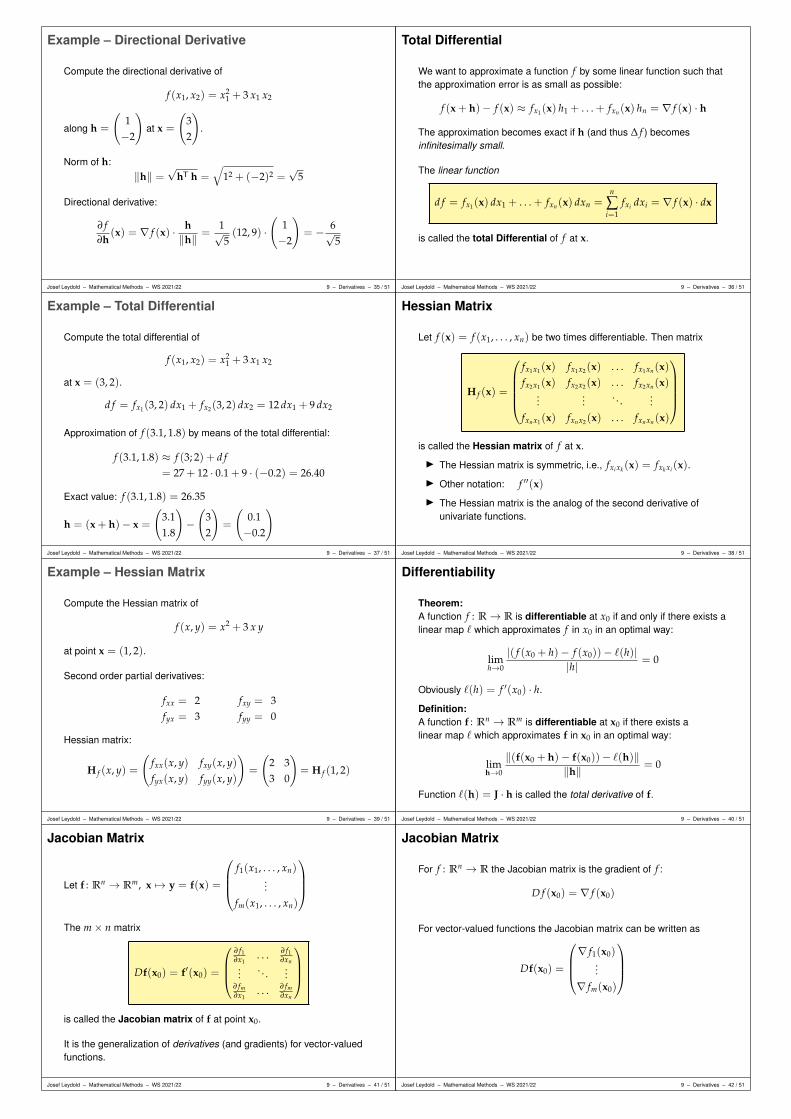
Example – Directional Derivative
Compute the directional derivative of
f (x1, x2) = x21 + 3 x1 x2
along h =
(1−2
)at x =
(32
).
Norm of h:‖h‖ =
√hT h =
√12 + (−2)2 =
√5
Directional derivative:
∂ f∂h
(x) = ∇ f (x) · h‖h‖ =
1√5(12, 9) ·
(1−2
)= − 6√
5
Josef Leydold – Mathematical Methods – WS 2021/22 9 – Derivatives – 35 / 51
Total Differential
We want to approximate a function f by some linear function such thatthe approximation error is as small as possible:
f (x + h)− f (x) ≈ fx1(x) h1 + . . . + fxn(x) hn = ∇ f (x) · h
The approximation becomes exact if h (and thus ∆ f ) becomesinfinitesimally small.
The linear function
d f = fx1(x) dx1 + . . . + fxn(x) dxn =n
∑i=1
fxi dxi = ∇ f (x) · dx
is called the total Differential of f at x.
Josef Leydold – Mathematical Methods – WS 2021/22 9 – Derivatives – 36 / 51
Example – Total Differential
Compute the total differential of
f (x1, x2) = x21 + 3 x1 x2
at x = (3, 2).
d f = fx1(3, 2) dx1 + fx2(3, 2) dx2 = 12 dx1 + 9 dx2
Approximation of f (3.1, 1.8) by means of the total differential:
f (3.1, 1.8) ≈ f (3; 2) + d f= 27 + 12 · 0.1 + 9 · (−0.2) = 26.40
Exact value: f (3.1, 1.8) = 26.35
h = (x + h)− x =
(3.11.8
)−(
32
)=
(0.1−0.2
)
Josef Leydold – Mathematical Methods – WS 2021/22 9 – Derivatives – 37 / 51
Hessian Matrix
Let f (x) = f (x1, . . . , xn) be two times differentiable. Then matrix
H f (x) =
fx1x1(x) fx1x2(x) . . . fx1xn(x)fx2x1(x) fx2x2(x) . . . fx2xn(x)
......
. . ....
fxnx1(x) fxnx2(x) . . . fxnxn(x)
is called the Hessian matrix of f at x.
I The Hessian matrix is symmetric, i.e., fxixk(x) = fxkxi(x).
I Other notation: f ′′(x)
I The Hessian matrix is the analog of the second derivative ofunivariate functions.
Josef Leydold – Mathematical Methods – WS 2021/22 9 – Derivatives – 38 / 51
Example – Hessian Matrix
Compute the Hessian matrix of
f (x, y) = x2 + 3 x y
at point x = (1, 2).
Second order partial derivatives:
fxx = 2 fxy = 3fyx = 3 fyy = 0
Hessian matrix:
H f (x, y) =
(fxx(x, y) fxy(x, y)fyx(x, y) fyy(x, y)
)=
(2 33 0
)= H f (1, 2)
Josef Leydold – Mathematical Methods – WS 2021/22 9 – Derivatives – 39 / 51
Differentiability
Theorem:A function f : R→ R is differentiable at x0 if and only if there exists alinear map ` which approximates f in x0 in an optimal way:
limh→0
|( f (x0 + h)− f (x0))− `(h)||h| = 0
Obviously `(h) = f ′(x0) · h.
Definition:A function f : Rn → Rm is differentiable at x0 if there exists alinear map ` which approximates f in x0 in an optimal way:
limh→0
‖(f(x0 + h)− f(x0))− `(h)‖‖h‖ = 0
Function `(h) = J · h is called the total derivative of f.
Josef Leydold – Mathematical Methods – WS 2021/22 9 – Derivatives – 40 / 51
Jacobian Matrix
Let f : Rn → Rm, x 7→ y = f(x) =
f1(x1, . . . , xn)...
fm(x1, . . . , xn)
The m× n matrix
Df(x0) = f′(x0) =
∂ f1∂x1
. . . ∂ f1∂xn
.... . .
...∂ fm∂x1
. . . ∂ fm∂xn
is called the Jacobian matrix of f at point x0.
It is the generalization of derivatives (and gradients) for vector-valuedfunctions.
Josef Leydold – Mathematical Methods – WS 2021/22 9 – Derivatives – 41 / 51
Jacobian Matrix
For f : Rn → R the Jacobian matrix is the gradient of f :
D f (x0) = ∇ f (x0)
For vector-valued functions the Jacobian matrix can be written as
Df(x0) =
∇ f1(x0)...
∇ fm(x0)
Josef Leydold – Mathematical Methods – WS 2021/22 9 – Derivatives – 42 / 51

Example – Jacobian Matrix
I f (x) = f (x1, x2) = exp(−x21 − x2
2)
D f (x) =(
∂ f∂x1
, ∂ f∂x2
)= ∇ f (x)
=(−2 x1 exp(−x2
1 − x22),−2 x2 exp(−x2
1 − x22))
I f(x) = f(x1, x2) =
(f1(x1, x2)
f2(x1, x2)
)=
(x2
1 + x22
x21 − x2
2
)
Df(x) =
( ∂ f1∂x1
∂ f1∂x2
∂ f2∂x1
∂ f2∂x2
)=
(2 x1 2 x2
2 x1 −2 x2
)
I s(t) =
(s1(t)s2(t)
)=
(cos(t)sin(t)
)
Ds(t) =
(ds1dtds2dt
)=
(− sin(t)cos(t)
)
Josef Leydold – Mathematical Methods – WS 2021/22 9 – Derivatives – 43 / 51
Chain Rule
Let f : Rn → Rm and g : Rm → Rk. Then
(g f)′(x) = g′(f(x)) · f′(x)
f(x, y) =
(ex
ey
)g(x, y) =
(x2 + y2
x2 − y2
)
f′(x, y) =
(ex 00 ey
)g′(x, y) =
(2 x 2 y2 x −2 y
)
(g f)′(x) = g′(f(x)) · f′(x) =(
2 ex 2 ey
2 ex −2 ey
)·(
ex 00 ey
)
=
(2 e2x 2 e2y
2 e2x −2 e2y
)
Josef Leydold – Mathematical Methods – WS 2021/22 9 – Derivatives – 44 / 51
Example – Directional Derivative
We can derive the formula for the directional derivative of f : Rn → R
along h (with ‖h‖ = 1) at x0 by means of the chain rule:
Let s(t) be a path through x0 along h, i.e.,
s : R→ Rn, t 7→ x0 + th .
Thenf ′(s(0)) = f ′(x0) = ∇ f (x0)
s′(0) = h
and hence
∂ f∂h
= ( f s)′(0) = f ′(s(0)) · s′(0) = ∇ f (x0) · h .
Josef Leydold – Mathematical Methods – WS 2021/22 9 – Derivatives – 45 / 51
Example – Indirect Dependency
Let f (x1, x2, t) where x1(t) and x2(t) also depend on t.What is the total derivative of f w.r.t. t?
Chain rule:
Let x : R→ R3, t 7→
x1(t)x2(t)
t
d fdt
= ( f x)′(t) = f ′(x(t)) · x′(t)
= ∇ f (x(t)) ·
x′1(t)x′2(t)
1
=( fx1(x(t)), fx2(x(t)), ft(x(t)) ·
x′1(t)x′2(t)
1
= fx1(x(t)) · x′1(t) + fx2(x(t)) · x′2(t) + ft(x(t))
= fx1(x1, x2, t) · x′1(t) + fx2(x1, x2, t) · x′2(t) + ft(x1, x2, t)
Josef Leydold – Mathematical Methods – WS 2021/22 9 – Derivatives – 46 / 51
L’Hôpital’s Rule
Suppose we want to compute
limx→x0
f (x)g(x)
and findlim
x→x0f (x) = lim
x→x0g(x) = 0 (or = ±∞)
However, expressions like 00 or ∞
∞ are not defined.
(You must not reduce the fraction by 0 or ∞!)
Josef Leydold – Mathematical Methods – WS 2021/22 9 – Derivatives – 47 / 51
L’Hôpital’s Rule
If limx→x0
f (x) = limx→x0
g(x) = 0 (or = ∞ or = −∞), then
limx→x0
f (x)g(x)
= limx→x0
f ′(x)g′(x)
Assumption: f and g are differentiable in x0.
This formula is called l’Hôpital’s rule (also spelled as l’Hospital’s rule).
Josef Leydold – Mathematical Methods – WS 2021/22 9 – Derivatives – 48 / 51
Example – L’Hôpital’s Rule
limx→2
x3 − 7 x + 6x2 − x− 2
= limx→2
3 x2 − 72 x− 1
=53
limx→∞
ln xx2 = lim
x→∞
1x
2 x= lim
x→∞
12 x2 = 0
limx→0
x− ln(1 + x)x2 = lim
x→0
1− (1 + x)−1
2 x= lim
x→0
(1 + x)−2
2=
12
Josef Leydold – Mathematical Methods – WS 2021/22 9 – Derivatives – 49 / 51
Example – L’Hôpital’s Rule
L’Hôpital’s rule can be applied iteratively:
limx→0
ex − x− 1x2 = lim
x→0
ex − 12x
= limx→0
ex
2=
12
Josef Leydold – Mathematical Methods – WS 2021/22 9 – Derivatives – 50 / 51

Summary
I difference quotient and differential quotientI differential quotient and derivativeI derivatives of elementary functionsI differentiation rulesI higher order derivativesI total differentialI elasticityI partial derivativesI gradient and Hessian matrixI Jacobian matrix and chain ruleI l’Hôpital’s rule
Josef Leydold – Mathematical Methods – WS 2021/22 9 – Derivatives – 51 / 51
Chapter 10
Inverse and ImplicitFunctions
Josef Leydold – Mathematical Methods – WS 2021/22 10 – Inverse and Implicit Functions – 1 / 23
Inverse Function
Let f : D f ⊆ Rn →W f ⊆ Rm, x 7→ y = f(x). A Function
f−1 : W f → D f , y 7→ x = f−1(y)
is called inverse function of f, if
f−1 f = f f−1 = id
where id denotes the identity function, id(x) = x:
f−1(f(x)) = f−1(y) = x and f(f−1(y)) = f(x) = y
f−1 exists if and only if f is bijective.
We then obtain f−1(y) as the unique solution x of equation y = f(x).
Josef Leydold – Mathematical Methods – WS 2021/22 10 – Inverse and Implicit Functions – 2 / 23
Linear Function
Let f : R→ R, x 7→ y = f (x) = a x + b.
y = a x + b ⇔ a x = y− b ⇔ x = 1a y− b
a
That is,f−1(y) = a−1 y− a−1 b
Provided that a 6= 0 [ a = f ′(x) ]
Observe:
( f−1)′(y) = a−1 =1a=
1f ′(x)
Josef Leydold – Mathematical Methods – WS 2021/22 10 – Inverse and Implicit Functions – 3 / 23
Linear Function
Let f : Rn → Rm, x 7→ y = f(x) = A x + b for some m× n matrix A.
y = A x + b ⇔ x = A−1 y−A−1 b
That is,f−1(y) = A−1 y−A−1 b .
Provided that A is invertible, [ A = Df(x) ](and thus: n = m)
Observe:(f−1)′(y) = A−1 = (f′(x))−1
Josef Leydold – Mathematical Methods – WS 2021/22 10 – Inverse and Implicit Functions – 4 / 23
Locally Invertible Function
Function
f : R→ [0, ∞), x 7→ f (x) = x2
is not bijective. Thusf−1 does not exist globally.
For some x0 there exists an openinterval (x0 − ε, x0 + ε) wherey = f (x) can be solved w.r.t. x.
We say:f is locally invertible around x0.
For other x0 such an interval doesnot exist (even if it is very short).
x− ε x + ε
locally invertible
y
x
not locally invertible
Josef Leydold – Mathematical Methods – WS 2021/22 10 – Inverse and Implicit Functions – 5 / 23
Existence and Derivative
1. For which x0 is f locallyinvertible?
2. What is the derivative of f−1 aty0 = f(x0).
Idea:Replace f by its differential:
f(x0 + h) ≈ f(x0) + f′(x0) · h
Hence:
1. f′(x0) must be invertible.
2. (f−1)′(y0) = (f′(x0))−1
locally invertible
x0
not locally invertible
Josef Leydold – Mathematical Methods – WS 2021/22 10 – Inverse and Implicit Functions – 6 / 23
Inverse Function Theorem
Let f : D f ⊆ R→ R be a function and x0 some point with f ′(x0) 6= 0.
Then there exist open intervals U around x0 and V around y0 = f (x0)such that f : U → V is one-to-one and onto,i.e., the inverse function f−1 : V → U exists.
Moreover, we find for its derivative:
( f−1)′(y0) =1
f ′(x0)
Josef Leydold – Mathematical Methods – WS 2021/22 10 – Inverse and Implicit Functions – 7 / 23
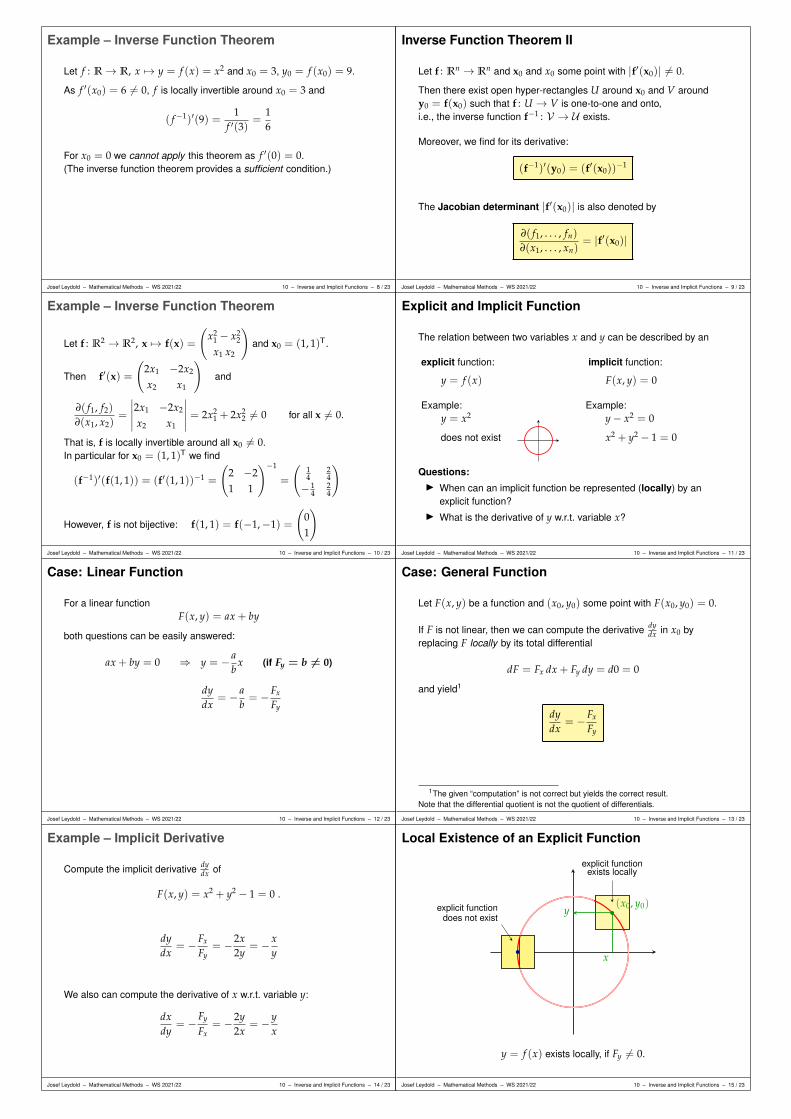
Example – Inverse Function Theorem
Let f : R→ R, x 7→ y = f (x) = x2 and x0 = 3, y0 = f (x0) = 9.
As f ′(x0) = 6 6= 0, f is locally invertible around x0 = 3 and
( f−1)′(9) =1
f ′(3)=
16
For x0 = 0 we cannot apply this theorem as f ′(0) = 0.(The inverse function theorem provides a sufficient condition.)
Josef Leydold – Mathematical Methods – WS 2021/22 10 – Inverse and Implicit Functions – 8 / 23
Inverse Function Theorem II
Let f : Rn → Rn and x0 and x0 some point with |f′(x0)| 6= 0.
Then there exist open hyper-rectangles U around x0 and V aroundy0 = f(x0) such that f : U → V is one-to-one and onto,i.e., the inverse function f−1 : V → U exists.
Moreover, we find for its derivative:
(f−1)′(y0) = (f′(x0))−1
The Jacobian determinant |f′(x0)| is also denoted by
∂( f1, . . . , fn)
∂(x1, . . . , xn)= |f′(x0)|
Josef Leydold – Mathematical Methods – WS 2021/22 10 – Inverse and Implicit Functions – 9 / 23
Example – Inverse Function Theorem
Let f : R2 → R2, x 7→ f(x) =
(x2
1 − x22
x1 x2
)and x0 = (1, 1)T.
Then f′(x) =
(2x1 −2x2
x2 x1
)and
∂( f1, f2)
∂(x1, x2)=
∣∣∣∣∣2x1 −2x2
x2 x1
∣∣∣∣∣ = 2x21 + 2x2
2 6= 0 for all x 6= 0.
That is, f is locally invertible around all x0 6= 0.In particular for x0 = (1, 1)T we find
(f−1)′(f(1, 1)) = (f′(1, 1))−1 =
(2 −21 1
)−1
=
(14
24
− 14
24
)
However, f is not bijective: f(1, 1) = f(−1,−1) =
(01
)
Josef Leydold – Mathematical Methods – WS 2021/22 10 – Inverse and Implicit Functions – 10 / 23
Explicit and Implicit Function
The relation between two variables x and y can be described by an
explicit function:
y = f (x)
Example:y = x2
does not exist
implicit function:
F(x, y) = 0
Example:y− x2 = 0
x2 + y2 − 1 = 0
Questions:I When can an implicit function be represented (locally) by an
explicit function?I What is the derivative of y w.r.t. variable x?
Josef Leydold – Mathematical Methods – WS 2021/22 10 – Inverse and Implicit Functions – 11 / 23
Case: Linear Function
For a linear functionF(x, y) = ax + by
both questions can be easily answered:
ax + by = 0 ⇒ y = − ab
x (if Fy = b 6= 0)
dydx
= − ab= −Fx
Fy
Josef Leydold – Mathematical Methods – WS 2021/22 10 – Inverse and Implicit Functions – 12 / 23
Case: General Function
Let F(x, y) be a function and (x0, y0) some point with F(x0, y0) = 0.
If F is not linear, then we can compute the derivative dydx in x0 by
replacing F locally by its total differential
dF = Fx dx + Fy dy = d0 = 0
and yield1
dydx
= −Fx
Fy
1The given “computation” is not correct but yields the correct result.Note that the differential quotient is not the quotient of differentials.
Josef Leydold – Mathematical Methods – WS 2021/22 10 – Inverse and Implicit Functions – 13 / 23
Example – Implicit Derivative
Compute the implicit derivative dydx of
F(x, y) = x2 + y2 − 1 = 0 .
dydx
= −Fx
Fy= −2x
2y= − x
y
We also can compute the derivative of x w.r.t. variable y:
dxdy
= − Fy
Fx= −2y
2x= −y
x
Josef Leydold – Mathematical Methods – WS 2021/22 10 – Inverse and Implicit Functions – 14 / 23
Local Existence of an Explicit Function
explicit functionexists locally
y
x
(x0, y0)explicit functiondoes not exist
y = f (x) exists locally, if Fy 6= 0.
Josef Leydold – Mathematical Methods – WS 2021/22 10 – Inverse and Implicit Functions – 15 / 23

Implicit Function Theorem
Let F : R2 → R and let (x0, y0) be some point with
F(x0, y0) = 0 and Fy(x0, y0) 6= 0 .
Then there exists a rectangle R around (x0, y0) such that
I F(x, y) = 0 has a unique solution y = f (x) in R, and
I dydx
= −Fx
Fy
Josef Leydold – Mathematical Methods – WS 2021/22 10 – Inverse and Implicit Functions – 16 / 23
Example – Implicit Function Theorem
Let F(x, y) = x2 + y2 − 8 and (x0, y0) = (2, 2).
As F(x0, y0) = 0 and Fy(x0, y0) = 2 y0 = 4 6= 0,variable y can be represented locally as a function of variable x and
dydx
(x0) = −Fx(x0, y0)
Fy(x0, y0)= −2x0
2y0= −1 .
Josef Leydold – Mathematical Methods – WS 2021/22 10 – Inverse and Implicit Functions – 17 / 23
Implicit Function Theorem II
Let F : Rn+1 → R, (x, y) 7→ F(x, y) = F(x1, . . . , xn, y), andlet (x0, y0) be some point with
F(x0, y0) = 0 and Fy(x0, y0) 6= 0 .
Then there exists a hyper-rectangle R around (x0, y0) such that
I F(x, y) = 0 has a unique solution y = f (x) in R, wheref : Rn → R, and
I ∂y∂xi
= −Fxi
Fy
The independent variable y can be any of the variables of F and neednot be in the last position.
Josef Leydold – Mathematical Methods – WS 2021/22 10 – Inverse and Implicit Functions – 18 / 23
Example – Implicit Function Theorem
Compute ∂x2∂x3
of the implicit function
F(x1, x2, x3, x4) = x21 + x2 x3 + x2
3 − x3 x4 − 1 = 0
at point (x1, x2, x3, x4) = (1, 0, 1, 1).
As F(1, 0, 1, 1) = 0 and Fx2(1, 0, 1, 1) = 1 6= 0 we can represent x2locally as a function of (x1, x3, x4): x2 = f (x1, x3, x4).
The partial derivative w.r.t. x3 is given by
∂x2
∂x3= −Fx3
Fx2
= − x2 + 2 x3 − x4
x3= −1
At (1, 1, 1, 1) and (1, 1, 0, 1) the implicit function theorem cannot beapplied for independent variable x2:
F(1, 1, 1, 1) 6= 0 and Fx2(1, 1, 0, 1) = 0.
Josef Leydold – Mathematical Methods – WS 2021/22 10 – Inverse and Implicit Functions – 19 / 23
Jacobian Matrix
Let
F(x, y) =
F1(x1, . . . , xn, y1, . . . , ym)...
Fm(x1, . . . , xn, y1, . . . , ym)
= 0
then matrix
∂F(x, y)∂y
=
∂F1∂y1
. . . ∂F1∂ym
.... . .
...∂Fm∂y1
. . . ∂Fm∂ym
is called the Jacobian matrix of F(x, y) w.r.t. y.
Analogous: ∂F(x,y)∂x
Josef Leydold – Mathematical Methods – WS 2021/22 10 – Inverse and Implicit Functions – 20 / 23
Implicit Function Theorem III
Let F : Rn+m → Rm,
(x, y) 7→ F(x, y) =
F1(x1, . . . , xn, y1, . . . , ym)...
Fm(x1, . . . , xn, y1, . . . , ym)
and let (x0, y0) be a point with
F(x0, y0) = 0 and
∣∣∣∣∂F(x, y)
∂y
∣∣∣∣ 6= 0 for (x, y) = (x0, y0).
Then there exists a hyper-rectangle R around (x0, y0) such that
I F(x, y) = 0 has a unique solution y = f(x) in R, wheref : Rn → Rm, and
I ∂y∂x
= −(
∂F∂y
)−1
·(
∂F∂x
)
Josef Leydold – Mathematical Methods – WS 2021/22 10 – Inverse and Implicit Functions – 21 / 23
Example – Implicit Function Theorem
Let F(x, y) =
(F1(x1, x2, y1, y2)
F2(x1, x2, y1, y2)
)=
(x2
1 + x22 − y2
1 − y22 + 3
x31 + x3
2 + y31 + y3
2 − 11
)
and (x0, y0) = (1, 1, 1, 2).
∂F∂x
=
(∂F1∂x1
∂F1∂x2
∂F2∂x1
∂F2∂x2
)=
(2x1 2x2
3x21 3x2
2
)∂F∂x
(1, 1, 1, 2) =
(2 23 3
)
∂F∂y
=
(∂F1∂y1
∂F1∂y2
∂F2∂y1
∂F2∂y2
)=
(−2y1 −2y2
3y21 3y2
2
)∂F∂y
(1, 1, 1, 2) =
(−2 −43 12
)
As F(1, 1, 1, 2) = 0 and∣∣∣ ∂F(x,y)
∂y
∣∣∣ = −12 6= 0 we can apply the implicitfunction theorem and we find
∂y∂x
= −(
∂F∂y
)−1·(
∂F∂x
)= − 1
−12
(12 4−3 −2
)·(
2 23 3
)=
(3 30 0
)
Josef Leydold – Mathematical Methods – WS 2021/22 10 – Inverse and Implicit Functions – 22 / 23
Summary
I local existence of an inverse functionI derivative of an inverse FunctionI inverse function theoremI explicit and implicit functionI explicit representation of an implicit functionI derivative of an implicit functionI implicit function theorem
Josef Leydold – Mathematical Methods – WS 2021/22 10 – Inverse and Implicit Functions – 23 / 23
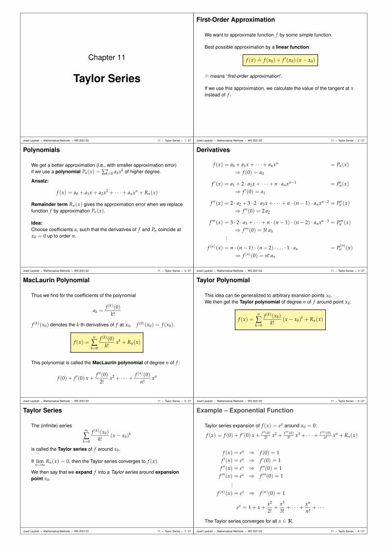
Chapter 11
Taylor Series
Josef Leydold – Mathematical Methods – WS 2021/22 11 – Taylor Series – 1 / 27
First-Order Approximation
We want to approximate function f by some simple function.
Best possible approximation by a linear function:
f (x) .= f (x0) + f ′(x0) (x− x0)
.= means “first-order approximation”.
If we use this approximation, we calculate the value of the tangent at xinstead of f .
Josef Leydold – Mathematical Methods – WS 2021/22 11 – Taylor Series – 2 / 27
Polynomials
We get a better approximation (i.e., with smaller approximation error)if we use a polynomial Pn(x) = ∑n
k=0 akxk of higher degree.
Ansatz:
f (x) = a0 + a1x + a2x2 + · · ·+ anxn + Rn(x)
Remainder term Rn(x) gives the approximation error when we replacefunction f by approximation Pn(x).
Idea:Choose coefficients ai such that the derivatives of f and Pn coincide atx0 = 0 up to order n.
Josef Leydold – Mathematical Methods – WS 2021/22 11 – Taylor Series – 3 / 27
Derivatives
f (x) = a0 + a1x + · · ·+ anxn = Pn(x)⇒ f (0) = a0
f ′(x) = a1 + 2 · a2x + · · ·+ n · anxn−1 = P′n(x)⇒ f ′(0) = a1
f ′′(x) = 2 · a2 + 3 · 2 · a3x + · · ·+ n · (n− 1) · anxn−2 = P′′n (x)⇒ f ′′(0) = 2 a2
f ′′′(x) = 3 · 2 · a3 + · · ·+ n · (n− 1) · (n− 2) · anxn−3 = P′′′n (x)⇒ f ′′′(0) = 3! a3
...
f (n)(x) = n · (n− 1) · (n− 2) · . . . · 1 · an = P(n)n (x)
⇒ f (n)(0) = n! an
Josef Leydold – Mathematical Methods – WS 2021/22 11 – Taylor Series – 4 / 27
MacLaurin Polynomial
Thus we find for the coefficients of the polynomial
ak =f (k)(0)
k!
f (k)(x0) denotes the k-th derivatives of f at x0, f (0)(x0) = f (x0).
f (x) =n
∑k=0
f (k)(0)k!
xk + Rn(x)
This polynomial is called the MacLaurin polynomial of degree n of f :
f (0) + f ′(0) x +f ′′(0)
2!x2 + · · ·+ f (n)(0)
n!xn
Josef Leydold – Mathematical Methods – WS 2021/22 11 – Taylor Series – 5 / 27
Taylor Polynomial
This idea can be generalized to arbitrary exansion points x0.We then get the Taylor polynomial of degree n of f around point x0:
f (x) =n
∑k=0
f (k)(x0)
k!(x− x0)
k + Rn(x)
Josef Leydold – Mathematical Methods – WS 2021/22 11 – Taylor Series – 6 / 27
Taylor Series
The (infinite) series∞
∑k=0
f (k)(x0)
k!(x− x0)
k
is called the Taylor series of f around x0.
If limn→∞
Rn(x) = 0, then the Taylor series converges to f (x).
We then say that we expand f into a Taylor series around expansionpoint x0.
Josef Leydold – Mathematical Methods – WS 2021/22 11 – Taylor Series – 7 / 27
Example – Exponential Function
Taylor series expansion of f (x) = ex around x0 = 0:
f (x) = f (0) + f ′(0) x + f ′′(0)2! x2 + f ′′′(0)
3! x3 + · · ·+ f (n)(0)n! xn + Rn(x)
f (x) = ex ⇒ f (0) = 1f ′(x) = ex ⇒ f ′(0) = 1f ′′(x) = ex ⇒ f ′′(0) = 1f ′′′(x) = ex ⇒ f ′′′(0) = 1
...
f (n)(x) = ex ⇒ f (n)(0) = 1
ex = 1 + x +x2
2!+
x3
3!+ · · ·+ xn
n!+ · · ·
The Taylor series converges for all x ∈ R.
Josef Leydold – Mathematical Methods – WS 2021/22 11 – Taylor Series – 8 / 27

Example – Exponential Function
exp(x) = 1 + x +x2
2!+
x3
3!+
x4
4!+
x5
5!+
x6
6!+ · · ·
1
1
exp(x)
n = 1
n = 2
n = 3n = 4
Josef Leydold – Mathematical Methods – WS 2021/22 11 – Taylor Series – 9 / 27
Example – Logarithm
Taylor series expansion of f (x) = ln(1 + x) around x0 = 0:
f (x) = f (0) + f ′(0) x + f ′′(0)2! x2 + f ′′′(0)
3! x3 + · · ·+ f (n)(0)n! xn + Rn(x)
f (x) = ln(1 + x) ⇒ f (0) = 0f ′(x) = (1 + x)−1 ⇒ f ′(0) = 1f ′′(x) = −1 · (1 + x)−2 ⇒ f ′′(0) = −1f ′′′(x) = 2 · 1 · (1 + x)−3 ⇒ f ′′′(0) = 2!
...
f (n)(x) = (−1)n−1(n− 1)!(1 + x)−n+1⇒ f (n)(0) = (−1)n−1(n− 1)!
ln(1 + x) = x− x2
2+
x3
3− x4
4+ · · ·+ (−1)n−1 xn
n+ · · ·
The Taylor series converges for all x ∈ (−1, 1).
Josef Leydold – Mathematical Methods – WS 2021/22 11 – Taylor Series – 10 / 27
Example – Logarithm
ln(1 + x) = x− x2
2+
x3
3− x4
4+
x5
5− x6
6+ · · ·
1−1
1 ln(1 + x)
n = 1
n = 2
n = 5
n = 6
Josef Leydold – Mathematical Methods – WS 2021/22 11 – Taylor Series – 11 / 27
Radius of Convergence
Some Taylor series do not converge for all x ∈ R.For example: ln(1 + x)
At least the following holds:
If a Taylor series converges for some x1 with |x1 − x0| = ρ,then it also converges for all x with |x− x0| < ρ.
The maximal value for ρ is called the radius of convergence of theTaylor series.
ρ
x0 x1
Taylor series converges
Josef Leydold – Mathematical Methods – WS 2021/22 11 – Taylor Series – 12 / 27
Example – Radius of Convergence
ln(1 + x) = x− x2
2+
x3
3− x4
4+
x5
5− x6
6+ · · ·
Radius of convergence: ρ = 1
Indication:ln(1 + x) is not defined for x ≤ −1.
1−1
1
ρ
ρ
ln(1 + x)
n = 1n = 5
n = 7
n = 11n = 31
Josef Leydold – Mathematical Methods – WS 2021/22 11 – Taylor Series – 13 / 27
Approximation Error
The remainder term indicates the error of the approximation by a Taylorpolynomial.It can be estimated by means of Lagrange’s form of the remainder:
Rn(x) =f (n+1)(ξ)
(n + 1)!(x− x0)
n+1
for some point ξ ∈ (x, x0).
If the Taylor series converges we have
Rn(x) = O((x− x0)
n+1)
for x → x0
We say: the remainder is of big O of xn+1 as x tends to x0.
Josef Leydold – Mathematical Methods – WS 2021/22 11 – Taylor Series – 14 / 27
Big O Notation
Let f (x) and g(x) be two functions.
f (x)
g(x)
C g(x)
−C g(x)
We write
f (x) = O(
g(x))
as x → x0
if there exist reals numbers C and ε such that
| f (x)| < C · |g(x)|for all x with |x− x0| < ε.
We say that f (x) is of big O of g(x) as x tends to x0.
Symbol O(·) belongs to the family of Bachmann-Landau notations.
Some books use notation f (x) ∈ O(
g(x))
as x → x0
Josef Leydold – Mathematical Methods – WS 2021/22 11 – Taylor Series – 15 / 27
Impact of Order of Powers
The higher the order of a monomial is,the smaller is its contribution to the summation.
0.3
0.2x1 x2 x3
x4
x5
x6
x7
x8
Josef Leydold – Mathematical Methods – WS 2021/22 11 – Taylor Series – 16 / 27
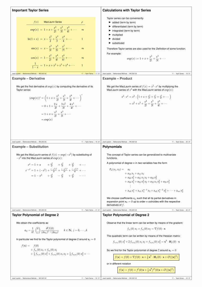
Important Taylor Series
f (x) MacLaurin Series ρ
exp(x) = 1 + x +x2
2!+
x3
3!+
x4
4!+ · · · ∞
ln(1 + x) = x− x2
2+
x3
3− x4
4+ · · · 1
sin(x) = x− x3
3!+
x5
5!− x7
7!+ · · · ∞
cos(x) = 1− x2
2!+
x4
4!− x6
6!+ · · · ∞
11− x
= 1 + x + x2 + x3 + x4 + · · · 1
Josef Leydold – Mathematical Methods – WS 2021/22 11 – Taylor Series – 17 / 27
Calculations with Taylor Series
Taylor series can be convenientlyI added (term by term)I differentiated (term by term)I integrated (term by term)I multipliedI dividedI substituted
Therefore Taylor series are also used for the Definition of some function.
For example:
exp(x) := 1 + x +x2
2!+
x3
3!+ · · ·
Josef Leydold – Mathematical Methods – WS 2021/22 11 – Taylor Series – 18 / 27
Example – Derivative
We get the first derivative of exp(x) by computing the derivative of itsTaylor series:
(exp(x))′ =(
1 + x +x2
2!+
x3
3!+
x4
4!+ · · ·
)′
= 0 + 1 +2 x2!
+3 x2
3!+
4 x3
4!+ · · ·
= 1 + x +x2
2!+
x3
3!+ · · ·
= exp(x)
Josef Leydold – Mathematical Methods – WS 2021/22 11 – Taylor Series – 19 / 27
Example – Product
We get the MacLaurin series of f (x) = x2 · ex by multiplying theMacLaurin series of x2 with the MacLaurin series of exp(x):
x2 · ex = x2 ·(
1 + x + x2
2! +x3
3! +x4
4! + · · ·)
= x2 + x3 +x4
2!+
x5
3!+
x6
4!+ · · ·
Josef Leydold – Mathematical Methods – WS 2021/22 11 – Taylor Series – 20 / 27
Example – Substitution
We get the MacLaurin series of f (x) = exp(−x2) by substituting of−x2 into the MacLaurin series of exp(x):
eu = 1 + u + u2
2! + u3
3! + u4
4! + · · ·
e−x2= 1 + (−x2) + (−x2)2
2! + (−x2)3
3! + (−x2)4
4! + · · ·= 1 − x2 + x4
2! − x6
3! + x8
4! − · · ·
Josef Leydold – Mathematical Methods – WS 2021/22 11 – Taylor Series – 21 / 27
Polynomials
The concept of Taylor series can be generalized to multivariatefunctions.
A polynomial of degree n in two variables has the form
Pn(x1, x2) = a0
+ a10 x1 + a11 x2
+ a20 x21 + a21 x1 x2 + a22 x2
2
+ a30 x31 + a31 x2
1 x2 + a32 x1 x22 + a33 x3
2...
+ an0 xn1 + an1 xn−1
1 x2 + an2 xn−21 x2
2 + · · ·+ ann xn2
We choose coefficients akj such that all its partial derivatives inexpansion point x0 = 0 up to order n coincides with the respectivederivatives of f .
Josef Leydold – Mathematical Methods – WS 2021/22 11 – Taylor Series – 22 / 27
Taylor Polynomial of Degree 2
We obtain the coefficients as
akj =1k!
(kj
)∂k f (0)
(∂x1)k−j (∂x2)j k ∈N, j = 0, · · · , k
In particular we find for the Taylor polynomial of degree 2 around x0 = 0
f (x) = f (0)+ fx1(0) x1 + fx2(0) x2
+ 12 fx1x1(0) x2
1 + fx1x2(0) x1 x2 +12 fx2x2(0) x2
2 + · · ·
Josef Leydold – Mathematical Methods – WS 2021/22 11 – Taylor Series – 23 / 27
Taylor Polynomial of Degree 2
Observe that the linear term can be written by means of the gradient:
fx1(0) x1 + fx2(0) x2 = ∇ f (0) · x
The quadratic term can be written by means of the Hessian matrix:
fx1x1(0) x21 + 2 fx1x2(0) x1 x2 + fx2x2(0) x2
2 = xT ·H f (0) · x
So we find for the Taylor polynomial of degree 2 around x0 = 0
f (x) = f (0) +∇ f (0) · x + 12 xT ·H f (0) · x +O(‖x‖3)
or in different notation
f (x) = f (0) + f ′(0)x + 12 xT f ′′(0)x +O(‖x‖3)
Josef Leydold – Mathematical Methods – WS 2021/22 11 – Taylor Series – 24 / 27
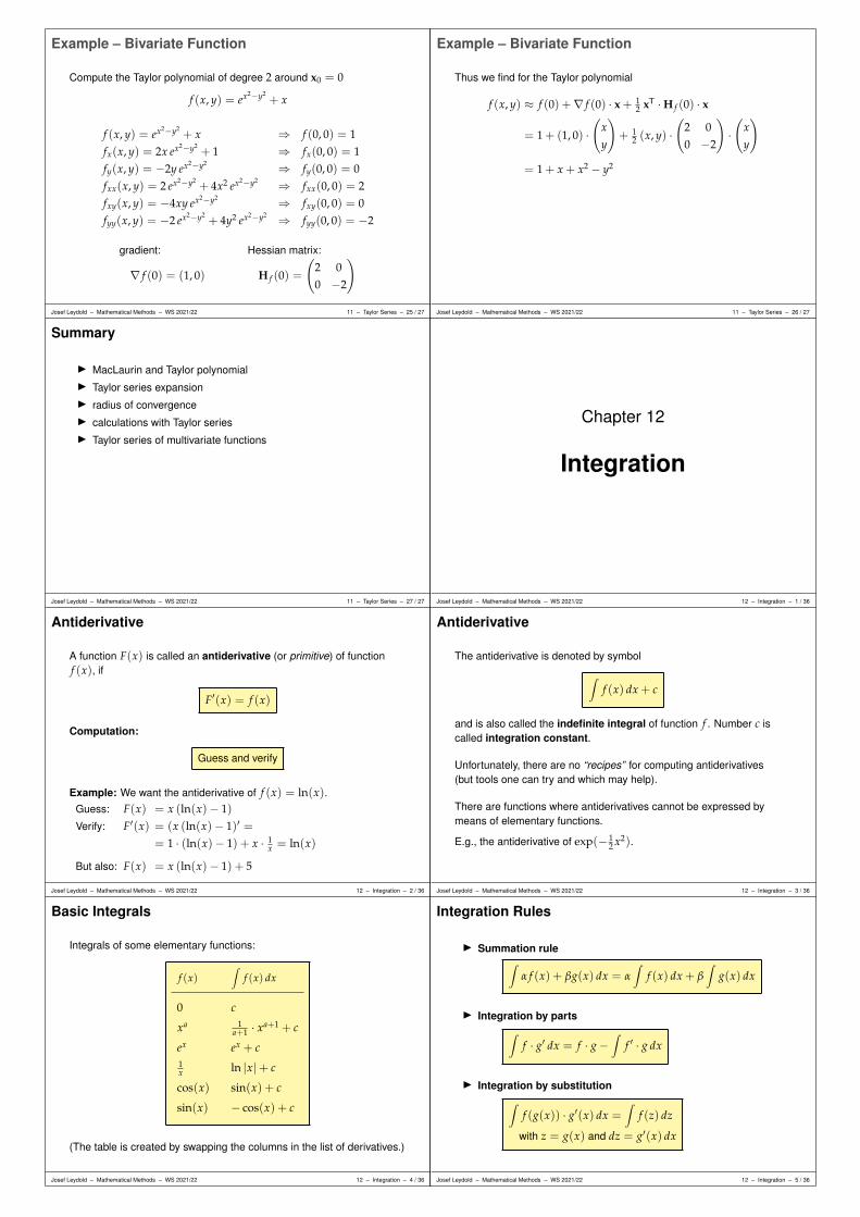
Example – Bivariate Function
Compute the Taylor polynomial of degree 2 around x0 = 0
f (x, y) = ex2−y2+ x
f (x, y) = ex2−y2+ x ⇒ f (0, 0) = 1
fx(x, y) = 2x ex2−y2+ 1 ⇒ fx(0, 0) = 1
fy(x, y) = −2y ex2−y2 ⇒ fy(0, 0) = 0fxx(x, y) = 2 ex2−y2
+ 4x2 ex2−y2 ⇒ fxx(0, 0) = 2fxy(x, y) = −4xy ex2−y2 ⇒ fxy(0, 0) = 0fyy(x, y) = −2 ex2−y2
+ 4y2 ex2−y2 ⇒ fyy(0, 0) = −2
gradient: Hessian matrix:
∇ f (0) = (1, 0) H f (0) =
(2 00 −2
)
Josef Leydold – Mathematical Methods – WS 2021/22 11 – Taylor Series – 25 / 27
Example – Bivariate Function
Thus we find for the Taylor polynomial
f (x, y) ≈ f (0) +∇ f (0) · x + 12 xT ·H f (0) · x
= 1 + (1, 0) ·(
xy
)+ 1
2 (x, y) ·(
2 00 −2
)·(
xy
)
= 1 + x + x2 − y2
Josef Leydold – Mathematical Methods – WS 2021/22 11 – Taylor Series – 26 / 27
Summary
I MacLaurin and Taylor polynomialI Taylor series expansionI radius of convergenceI calculations with Taylor seriesI Taylor series of multivariate functions
Josef Leydold – Mathematical Methods – WS 2021/22 11 – Taylor Series – 27 / 27
Chapter 12
Integration
Josef Leydold – Mathematical Methods – WS 2021/22 12 – Integration – 1 / 36
Antiderivative
A function F(x) is called an antiderivative (or primitive) of functionf (x), if
F′(x) = f (x)
Computation:
Guess and verify
Example: We want the antiderivative of f (x) = ln(x).Guess: F(x) = x (ln(x)− 1)Verify: F′(x) = (x (ln(x)− 1)′ =
= 1 · (ln(x)− 1) + x · 1x = ln(x)
But also: F(x) = x (ln(x)− 1) + 5
Josef Leydold – Mathematical Methods – WS 2021/22 12 – Integration – 2 / 36
Antiderivative
The antiderivative is denoted by symbol
∫f (x) dx + c
and is also called the indefinite integral of function f . Number c iscalled integration constant.
Unfortunately, there are no “recipes” for computing antiderivatives(but tools one can try and which may help).
There are functions where antiderivatives cannot be expressed bymeans of elementary functions.
E.g., the antiderivative of exp(− 12 x2).
Josef Leydold – Mathematical Methods – WS 2021/22 12 – Integration – 3 / 36
Basic Integrals
Integrals of some elementary functions:
f (x)∫
f (x) dx
0 c
xa 1a+1 · xa+1 + c
ex ex + c1x ln |x|+ c
cos(x) sin(x) + c
sin(x) − cos(x) + c
(The table is created by swapping the columns in the list of derivatives.)
Josef Leydold – Mathematical Methods – WS 2021/22 12 – Integration – 4 / 36
Integration Rules
I Summation rule∫
α f (x) + βg(x) dx = α∫
f (x) dx + β∫
g(x) dx
I Integration by parts∫
f · g′ dx = f · g−∫
f ′ · g dx
I Integration by substitution∫
f (g(x)) · g′(x) dx =∫
f (z) dz
with z = g(x) and dz = g′(x) dx
Josef Leydold – Mathematical Methods – WS 2021/22 12 – Integration – 5 / 36

Example – Summation Rule
Antiderivative of f (x) = 4 x3 − x2 + 3 x− 5.
∫f (x) dx =
∫4 x3 − x2 + 3 x− 5 dx
= 4∫
x3 dx−∫
x2 dx + 3∫
x dx− 5∫
dx
= 414
x4 − 13
x3 + 312
x2 − 5x + c
= x4 − 13
x3 +32
x2 − 5x + c
Josef Leydold – Mathematical Methods – WS 2021/22 12 – Integration – 6 / 36
Example – Integration by Parts
Antiderivative of f (x) = x · ex.
∫x︸︷︷︸f
· ex︸︷︷︸
g′
dx = x︸︷︷︸f
· ex︸︷︷︸
g
−∫
1︸︷︷︸f ′
· ex︸︷︷︸
g
dx = x · ex − ex + c
f = x ⇒ f ′ = 1g′ = ex ⇒ g = ex
Josef Leydold – Mathematical Methods – WS 2021/22 12 – Integration – 7 / 36
Example – Integration by Parts
Antiderivative of f (x) = x2 cos(x).∫
x2︸︷︷︸
f
· cos(x)︸ ︷︷ ︸g′
dx = x2︸︷︷︸
f
· sin(x)︸ ︷︷ ︸g
−∫
2x︸︷︷︸f ′
· sin(x)︸ ︷︷ ︸g
dx
Integration by parts of the second terms yields:∫
2x︸︷︷︸f
· sin(x)︸ ︷︷ ︸g′
dx = 2x︸︷︷︸f
· (− cos(x))︸ ︷︷ ︸g
−∫
2︸︷︷︸f ′
· (− cos(x))︸ ︷︷ ︸g
dx
= −2x · cos(x)− 2 · (− sin(x)) + c
Thus the antiderivative of f is given by∫
x2 cos(x) dx = x2 sin(x) + 2x cos(x)− 2 sin(x) + c
Josef Leydold – Mathematical Methods – WS 2021/22 12 – Integration – 8 / 36
Example – Integration by Substitution
Antiderivative of f (x) = 2x · ex2.
∫exp( x2
︸︷︷︸g(x)
) · 2x︸︷︷︸g′(x)
dx =∫
exp(z) dz = ez + c = ex2+ c
z = g(x) = x2 ⇒ dz = g′(x) dx = 2x dx
Josef Leydold – Mathematical Methods – WS 2021/22 12 – Integration – 9 / 36
Integration Rules – Derivation
Integration by parts follows from the product rule for derivatives:
f (x) · g(x) =∫
( f (x) · g(x))′ dx =∫ (
f ′(x) g(x) + f (x) g′(x))
dx
=∫
f ′(x) g(x) dx +∫
f (x) g′(x) dx
Integration by substitution follows from the chain rule:Let F be an antiderivative of f and let z = g(x). Then
∫f (z) dz = F(z) = F(g(x)) =
∫(F(g(x)))′ dx
=∫
F′(g(x)) g′(x) dx =∫
f (g(x)) g′(x) dx
Josef Leydold – Mathematical Methods – WS 2021/22 12 – Integration – 10 / 36
Area
Compute the areas of the given regions.
1
1
f (x) = 1
Area: A = 1
1
1
f (x) = 11+x2
Approximationby step function
Josef Leydold – Mathematical Methods – WS 2021/22 12 – Integration – 11 / 36
Riemann Sum
x0 ξ1 x1 ξ2 x2
f (ξ1)
f (ξ2)
ξi =12 (xi−1 + xi)
in general: ξi ∈ (xi, xi−1)
A =∫ b
af (x) dx ≈
n
∑i=1
f (ξi) · (xi − xi−1)
Josef Leydold – Mathematical Methods – WS 2021/22 12 – Integration – 12 / 36
Approximation Error
x0 ξ1 x1 ξ2 x2
f (ξ1)
f (ξ2)
f (x0)
f (x1)
f (x2)
∣∣∣∣∣∫ b
af (x) dx−
n
∑i=1
f (ξi) · (xi − xi−1)
∣∣∣∣∣ ≤ ( fmax− fmin) (b− a)1n→ 0
Assumption: Function monotone; x0, x1, . . . , xn equidistant
Josef Leydold – Mathematical Methods – WS 2021/22 12 – Integration – 13 / 36

Riemann Integral
If all sequences of Riemann sums
In =n
∑i=1
f (ξi) · (xi − xi−1)
converge, then their (uniquely determined) limit is called the
Riemann integral of f and is denoted by∫ b
af (x) dx:
∫ b
af (x) dx = lim
n→∞
n
∑i=1
f (ξi) · (xi − xi−1)
Almost all functions in economics have a Riemann integral.
Josef Leydold – Mathematical Methods – WS 2021/22 12 – Integration – 14 / 36
Riemann Integral – Properties
∫ b
a(α f (x) + βg(x)) dx = α
∫ b
af (x) dx + β
∫ b
ag(x) dx
∫ b
af (x) dx = −
∫ a
bf (x) dx
∫ a
af (x) dx = 0
∫ c
af (x) dx =
∫ b
af (x) dx +
∫ c
bf (x) dx
∫ b
af (x) dx ≤
∫ b
ag(x) dx if f (x) ≤ g(x) for all x ∈ [a, b]
Josef Leydold – Mathematical Methods – WS 2021/22 12 – Integration – 15 / 36
Fundamental Theorem of Calculus
Let F(x) be an antiderivative of a continuous function f (x),then we find
∫ b
af (x) dx = F(x)
∣∣∣b
a= F(b)− F(a)
By this theorem we can compute Riemann integrals by means ofantiderivatives!
For that reason∫
f (x) dx is called an indefinite integral of f ; and∫ b
af (x) dx is called a definite integral of f .
Josef Leydold – Mathematical Methods – WS 2021/22 12 – Integration – 16 / 36
Example – Fundamental Theorem
Compute the integral of f (x) = x2 over interval [ 0, 1 ].
∫ 1
0x2 dx = 1
3 x3∣∣∣1
0= 1
3 · 13 − 13 · 03 =
13
Josef Leydold – Mathematical Methods – WS 2021/22 12 – Integration – 17 / 36
Fundamental Theorem / Proof Idea
Let A(x) be the area between the graph of a continuous function f andthe x-axis from 0 to x.
A(x)
x + hx
fmin
fmax
fmin · h ≤ A(x + h)− A(x) ≤ fmax · h
fmin ≤A(x + h)− A(x)
h≤ fmax
Limit for h→ 0: (limh→0
fmin = f (x))
f (x) ≤ limh→0
A(x + h)− A(x)h︸ ︷︷ ︸
=A′(x)
≤ f (x)
A′(x) = f (x)
i.e. A(x) is an antiderivative of f (x).
Josef Leydold – Mathematical Methods – WS 2021/22 12 – Integration – 18 / 36
Integration Rules / (Definite Integrals)
I Summation rule∫ b
aα f (x) + βg(x) dx = α
∫ b
af (x) dx + β
∫ b
ag(x) dx
I Integration by parts
∫ b
af · g′ dx = f · g
∣∣∣b
a−∫ b
af ′ · g dx
I Integration by Substitution
∫ b
af (g(x)) · g′(x) dx =
∫ g(b)
g(a)f (z) dz
with z = g(x) and dz = g′(x) dx
Josef Leydold – Mathematical Methods – WS 2021/22 12 – Integration – 19 / 36
Example – Integration by Parts
Compute the definite integral∫ 2
0x · ex dx.
∫ 2
0x︸︷︷︸f
· ex︸︷︷︸
g′
dx = x︸︷︷︸f
· ex︸︷︷︸
g
∣∣∣2
0−∫ 2
01︸︷︷︸f ′
· ex︸︷︷︸
g
dx
= x · ex∣∣∣2
0− ex
∣∣∣2
0= (2 · e2 − 0 · e0)− (e2 − e0)
= e2 + 1
Note: we also could use our indefinite integral from above,
∫ 2
0x · ex dx = (x · ex − ex)
∣∣∣2
0= (2 · e2 − e2)− (0 · e0 − e0) = e2 + 1
Josef Leydold – Mathematical Methods – WS 2021/22 12 – Integration – 20 / 36
Example – Integration by Substitution
Compute the definite integral∫ 10
e
1ln(x)
· 1x
dx.
∫ 10
e
1ln(x)
· 1x
dx =∫ ln(10)
1
1z
dz =
z = ln(x) ⇒ dz =1x
dx
= ln(z)∣∣∣ln(10)
1=
= ln(ln(10))− ln(1) ≈ 0.834
Josef Leydold – Mathematical Methods – WS 2021/22 12 – Integration – 21 / 36
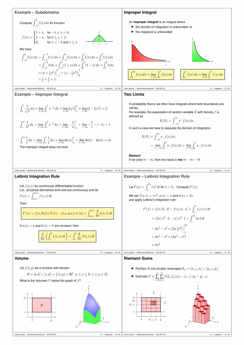
Example – Subdomains
Compute∫ 2
−2f (x) dx for function
f (x) =
1 + x, for −1 ≤ x < 0,1− x, for 0 ≤ x < 1,0, for x < −1 and x ≥ 1. −1 0 1
We have∫ 2
−2f (x) dx =
∫ −1
−2f (x) dx +
∫ 0
−1f (x) dx +
∫ 1
0f (x) dx +
∫ 2
1f (x) dx
=∫ −1
−20 dx +
∫ 0
−1(1 + x) dx +
∫ 1
0(1− x) dx +
∫ 2
10 dx
= (x + 12 x2)
∣∣∣0
−1+ (x− 1
2 x2)∣∣∣1
0
= 12 +
12 = 1
Josef Leydold – Mathematical Methods – WS 2021/22 12 – Integration – 22 / 36
Improper Integral
An improper integral is an integral whereI the domain of integration is unbounded, orI the integrand is unbounded.
t
∫ ∞
0f (x) dx = lim
t→∞
∫ t
0f (x) dx
∫ 1
0f (x) dx = lim
t→0
∫ 1
tf (x) dx
Josef Leydold – Mathematical Methods – WS 2021/22 12 – Integration – 23 / 36
Example – Improper Integral
∫ 1
0
1√x
dx = limt→0
∫ 1
tx−
12 dx = lim
t→02√
x∣∣∣1
t= lim
t→0(2− 2
√t) = 2
∫ ∞
1
1x2 dx = lim
t→∞
∫ t
1x−2 dx = lim
t→∞−1
x
∣∣∣∣t
1= lim
t→∞−1
t− (−1) = 1
∫ ∞
1
1x
dx = limt→∞
∫ t
1
1x
dx = limt→∞
ln(x)∣∣∣t
1= lim
t→∞ln(t)− ln(1) = ∞
The improper integral does not exist.
Josef Leydold – Mathematical Methods – WS 2021/22 12 – Integration – 24 / 36
Two Limits
In probability theory we often have integrals where both boundaries areinfinite.For example, the expectation of random variable X with density f isdefined as
E(X) =∫ ∞
−∞x · f (x) dx
In such a case we have to separate the domain of integration:
E(X) =∫ ∞
−∞x · f (x) dx
= limt→−∞
∫ 0
tx · f (x) dx + lim
s→∞
∫ s
0x · f (x) dx
Beware!If we yield ∞−∞, then the result is not ∞−∞ = 0!
Josef Leydold – Mathematical Methods – WS 2021/22 12 – Integration – 25 / 36
Leibniz Integration Rule
Let f (x, t) be continously differentiable function(i.e., all partial derivatives exist and are continuous) and let
F(x) =∫ b(x)
a(x)f (x, t) dt.
Then
F′(x) = f (x, b(x)) b′(x)− f (x, a(x)) a′(x) +∫ b(x)
a(x)
∂
∂xf (x, t) dt
If a(x) = a and b(x) = b are constant, then
ddx
(∫ b
af (x, t) dt
)=∫ b
a
∂
∂xf (x, t) dt
Josef Leydold – Mathematical Methods – WS 2021/22 12 – Integration – 26 / 36
Example – Leibniz Integration Rule
Let F(x) =∫ 2x
xt x2 dt for x > 0. Compute F′(x).
We set f (x, t) = t x2, a(x) = x and b(x) = 2xand apply Leibniz’s integration rule:
F′(x) = f (x, b) · b′ − f (x, a) · a′ +∫ b
afx(x, t) dt
= (2x) x2 · 2− (x) x2 · 1 +∫ 2x
x2x t dt
= 4x3 − x3 +(2x 1
2 t2)∣∣∣∣2x
x
= 4x3 − x3 + (4x3 − x3)
= 6x3
Josef Leydold – Mathematical Methods – WS 2021/22 12 – Integration – 27 / 36
Volume
Let f (x, y) be a function with domain
R = [a, b]× [c, d] = (x, y) ∈ R2 : a ≤ x ≤ b, c ≤ y ≤ dWhat is the Volumen V below the graph of f ?
a b
c
d
R
x
y
z
bd
Josef Leydold – Mathematical Methods – WS 2021/22 12 – Integration – 28 / 36
Riemann Sums
I Partition R into smaller rectangles Rij = [xi−1, xi]× [yj−1, yj]
I Estimate V ≈n
∑i=1
k
∑j=1
f (ξi, ζ j) (xi − xi−1) (yj − yj−1)
a b
c
d
xi−1 xi
yj−1
yj
ξi
ζi
x
y
z
bd
Josef Leydold – Mathematical Methods – WS 2021/22 12 – Integration – 29 / 36
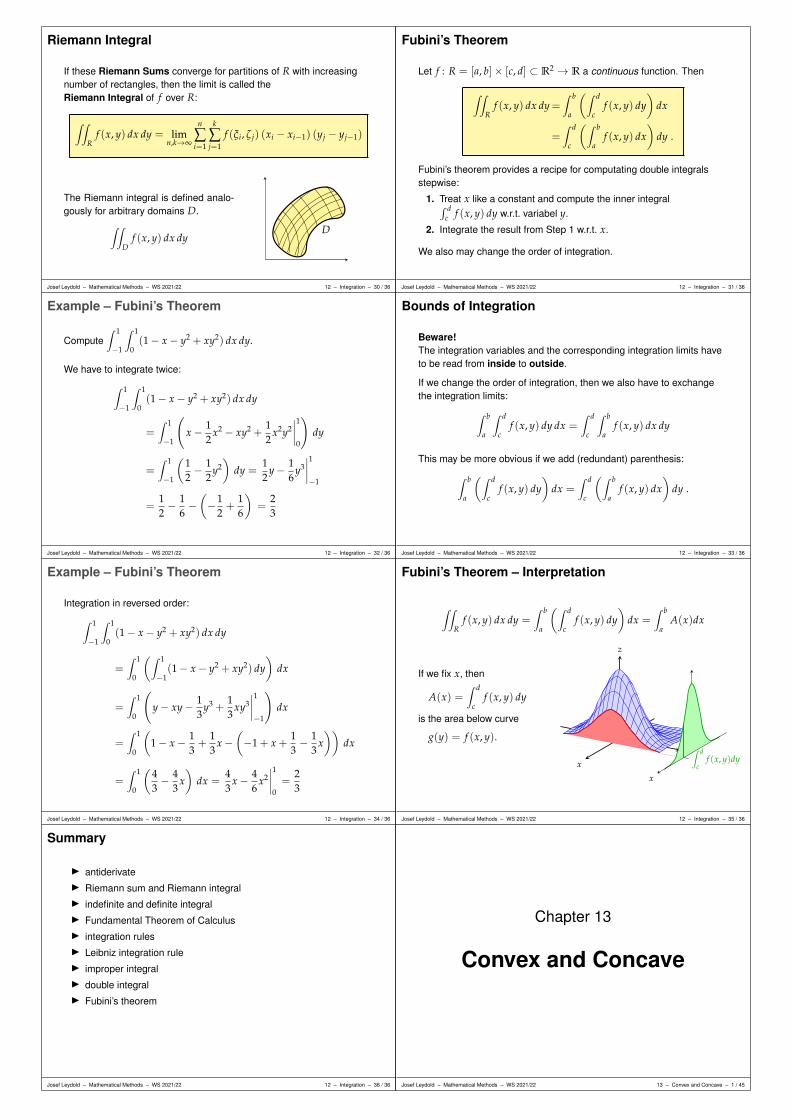
Riemann Integral
If these Riemann Sums converge for partitions of R with increasingnumber of rectangles, then the limit is called theRiemann Integral of f over R:
∫∫
Rf (x, y) dx dy = lim
n,k→∞
n
∑i=1
k
∑j=1
f (ξi, ζ j) (xi − xi−1) (yj − yj−1)
The Riemann integral is defined analo-gously for arbitrary domains D.
∫∫
Df (x, y) dx dy
D
Josef Leydold – Mathematical Methods – WS 2021/22 12 – Integration – 30 / 36
Fubini’s Theorem
Let f : R = [a, b]× [c, d] ⊂ R2 → R a continuous function. Then
∫∫
Rf (x, y) dx dy=
∫ b
a
(∫ d
cf (x, y) dy
)dx
=∫ d
c
(∫ b
af (x, y) dx
)dy .
Fubini’s theorem provides a recipe for computating double integralsstepwise:
1. Treat x like a constant and compute the inner integral∫ dc f (x, y) dy w.r.t. variabel y.
2. Integrate the result from Step 1 w.r.t. x.
We also may change the order of integration.
Josef Leydold – Mathematical Methods – WS 2021/22 12 – Integration – 31 / 36
Example – Fubini’s Theorem
Compute∫ 1
−1
∫ 1
0(1− x− y2 + xy2) dx dy.
We have to integrate twice:
∫ 1
−1
∫ 1
0(1− x− y2 + xy2) dx dy
=∫ 1
−1
(x− 1
2x2 − xy2 +
12
x2y2∣∣∣∣1
0
)dy
=∫ 1
−1
(12− 1
2y2)
dy =12
y− 16
y3∣∣∣∣1
−1
=12− 1
6−(−1
2+
16
)=
23
Josef Leydold – Mathematical Methods – WS 2021/22 12 – Integration – 32 / 36
Bounds of Integration
Beware!The integration variables and the corresponding integration limits haveto be read from inside to outside.
If we change the order of integration, then we also have to exchangethe integration limits:
∫ b
a
∫ d
cf (x, y) dy dx =
∫ d
c
∫ b
af (x, y) dx dy
This may be more obvious if we add (redundant) parenthesis:
∫ b
a
(∫ d
cf (x, y) dy
)dx =
∫ d
c
(∫ b
af (x, y) dx
)dy .
Josef Leydold – Mathematical Methods – WS 2021/22 12 – Integration – 33 / 36
Example – Fubini’s Theorem
Integration in reversed order:
∫ 1
−1
∫ 1
0(1− x− y2 + xy2) dx dy
=∫ 1
0
(∫ 1
−1(1− x− y2 + xy2) dy
)dx
=∫ 1
0
(y− xy− 1
3y3 +
13
xy3∣∣∣∣1
−1
)dx
=∫ 1
0
(1− x− 1
3+
13
x−(−1 + x +
13− 1
3x))
dx
=∫ 1
0
(43− 4
3x)
dx =43
x− 46
x2∣∣∣∣1
0=
23
Josef Leydold – Mathematical Methods – WS 2021/22 12 – Integration – 34 / 36
Fubini’s Theorem – Interpretation
∫∫
Rf (x, y) dx dy =
∫ b
a
(∫ d
cf (x, y) dy
)dx =
∫ b
aA(x)dx
If we fix x, then
A(x) =∫ d
cf (x, y) dy
is the area below curve
g(y) = f (x, y).y
x
z
∫ d
cf (x, y)dy
x
Josef Leydold – Mathematical Methods – WS 2021/22 12 – Integration – 35 / 36
Summary
I antiderivateI Riemann sum and Riemann integralI indefinite and definite integralI Fundamental Theorem of CalculusI integration rulesI Leibniz integration ruleI improper integralI double integralI Fubini’s theorem
Josef Leydold – Mathematical Methods – WS 2021/22 12 – Integration – 36 / 36
Chapter 13
Convex and Concave
Josef Leydold – Mathematical Methods – WS 2021/22 13 – Convex and Concave – 1 / 45

Monotone Functions∗
Function f is called monotonically increasing, if
x1 ≤ x2 ⇒ f (x1) ≤ f (x2)
It is called strictly monotonically increasing, if
x1 < x2 ⇔ f (x1) < f (x2) x1 x2
f (x1)
f (x2)
Function f is called monotonically decreasing, if
x1 ≤ x2 ⇒ f (x1) ≥ f (x2)
It is called strictly monotonically decreasing, if
x1 < x2 ⇔ f (x1) > f (x2) x1 x2
f (x1)
f (x2)
Josef Leydold – Mathematical Methods – WS 2021/22 13 – Convex and Concave – 2 / 45
Monotone Functions∗
For differentiable functions we have
f monotonically increasing ⇔ f ′(x) ≥ 0 for all x ∈ D f
f monotonically decreasing ⇔ f ′(x) ≤ 0 for all x ∈ D f
f strictly monotonically increasing ⇐ f ′(x) > 0 for all x ∈ D f
f strictly monotonically decreasing ⇐ f ′(x) < 0 for all x ∈ D f
Function f : (0, ∞), x 7→ ln(x) is strictly monotonically increasing, as
f ′(x) = (ln(x))′ =1x> 0 for all x > 0
Josef Leydold – Mathematical Methods – WS 2021/22 13 – Convex and Concave – 3 / 45
Locally Monotone Functions∗
A function f can be monotonically increasing in some interval anddecreasing in some other interval.
For continuously differentiable functions (i.e., when f ′(x) is continuous)we can use the following procedure:
1. Compute first derivative f ′(x).
2. Determine all roots of f ′(x).
3. We thus obtain intervals where f ′(x) does not change sign.
4. Select appropriate points xi in each interval and determine thesign of f ′(xi).
Josef Leydold – Mathematical Methods – WS 2021/22 13 – Convex and Concave – 4 / 45
Example – Locally Monotone Functions∗
In which region is function f (x) = 2 x3 − 12 x2 + 18 x− 1monotonically increasing?
We have to solve inequality f ′(x) ≥ 0:
1. f ′(x) = 6 x2 − 24 x + 18
2. Roots: x2 − 4 x + 3 = 0 ⇒ x1 = 1, x2 = 3
3. Obtain 3 intervals: (−∞, 1], [1, 3], and [3, ∞)
4. Sign of f ′(x) at appropriate points in each interval:f ′(0) = 3 > 0, f ′(2) = −1 < 0, and f ′(4) = 3 > 0.
5. f ′(x) cannot change sign in each interval:f ′(x) ≥ 0 in (−∞, 1] and [3, ∞).
Function f (x) is monotonically increasing in (−∞, 1] and in [3, ∞).
Josef Leydold – Mathematical Methods – WS 2021/22 13 – Convex and Concave – 5 / 45
Monotone and Inverse Function
If f is strictly monotonically increasing, then
x1 < x2 ⇔ f (x1) < f (x2)
immediately implies
x1 6= x2 ⇔ f (x1) 6= f (x2)
That is, f is one-to-one.
So if f is onto and strictly monotonically increasing (or decreasing),then f is invertible.
Josef Leydold – Mathematical Methods – WS 2021/22 13 – Convex and Concave – 6 / 45
Convex Set
A set D ⊆ Rn is called convex, if for any two points x, y ∈ D thestraight line segment between these points also belongs to D, i.e.,
(1− h) x + h y ∈ D for all h ∈ [0, 1], and x, y ∈ D .
convex:
not convex:
Josef Leydold – Mathematical Methods – WS 2021/22 13 – Convex and Concave – 7 / 45
Intersection of Convex Sets
Let S1, . . . , Sk be convex subsets of Rn. Then their intersectionS1 ∩ . . . ∩ Sk is also convex.
The union of convex sets need not be convex.
Josef Leydold – Mathematical Methods – WS 2021/22 13 – Convex and Concave – 8 / 45
Example – Half-Space
Let p ∈ Rn and m ∈ R be fixed, p 6= 0. Then
H = x ∈ Rn : pT · x = m
is a so called hyper-plane which partitions the Rn into two half-spaces
H+ = x ∈ Rn : pT · x ≥ m ,H− = x ∈ Rn : pT · x ≤ m .
Sets H, H+ and H− are convex.
Let x be a vector of goods, p the vector of prices and m the budget.Then the budget set is convex.
x ∈ Rn : pT · x ≤ m, x ≥ 0= x : pT · x ≤ m ∩ x : x1 ≥ 0 ∩ . . . ∩ x : xn ≥ 0
Josef Leydold – Mathematical Methods – WS 2021/22 13 – Convex and Concave – 9 / 45

Convex and Concave Functions
Function f is called convex in domain D ⊆ Rn, if D is convex and
f ((1− h) x1 + h x2) ≤ (1− h) f (x1) + h f (x2)
for all x1, x2 ∈ D and all h ∈ [0, 1]. It is called concave, if
f ((1− h) x1 + h x2) ≥ (1− h) f (x1) + h f (x2)
x1 x2 x1 x2
convex concave
Josef Leydold – Mathematical Methods – WS 2021/22 13 – Convex and Concave – 10 / 45
Concave Function∗
f((1− h) x1 + h x2
)≥ (1− h) f (x1) + h f (x2)
x1 x2(1− h) x1 + h x2
f((1− h) x1 + h x2
)
(1− h) f (x1) + h f (x2)
Secant is below the graph of function f .
Josef Leydold – Mathematical Methods – WS 2021/22 13 – Convex and Concave – 11 / 45
Strictly Convex and Concave Functions
Function f is strictly convex in domain D ⊆ Rn, if D is convex and
f ((1− h) x1 + h x2) < (1− h) f (x1) + h f (x2)
for all x1, x2 ∈ D with x1 6= x2 and all h ∈ (0, 1).
Function f is strictly concave in domain D ⊆ Rn, if D is convex and
f ((1− h) x1 + h x2) > (1− h) f (x1) + h f (x2)
for all x1, x2 ∈ D with x1 6= x2 and all h ∈ (0, 1).
Josef Leydold – Mathematical Methods – WS 2021/22 13 – Convex and Concave – 12 / 45
Example – Linear Function
Let a ∈ Rn be fixed.Then f (x) = aT · x is a linear map and we find:
f ((1− h) x1 + h x2) = aT · ((1− h) x1 + h x2)
= (1− h) aT · x1 + h aT · x2
= (1− h) f (x1) + h f (x2)
That is, every linear function is both concave and convex.
However, a linear function is neither strictly concave nor strictly convex,as the inequality is never strict.
Josef Leydold – Mathematical Methods – WS 2021/22 13 – Convex and Concave – 13 / 45
Example – Quadratic Univariate Function
Function f (x) = x2 is strictly convex :
f ((1− h) x + h y)−[(1− h) f (x) + h f (y)
]
= ((1− h) x + h y)2 −[(1− h) x2 + h y2]
= (1− h)2 x2 + 2(1− h)h xy + h2 y2 − (1− h) x2 − h y2
= −h(1− h) x2 + 2(1− h)h xy− h(1− h) y2
= −h(1− h) (x− y)2
< 0 for x 6= y and 0 < h < 1.
Thusf ((1− h) x + h y) < (1− h) f (x) + h f (y)
for all x 6= y and 0 < h < 1,i.e., f (x) = x2 is strictly convex, as claimed.
Josef Leydold – Mathematical Methods – WS 2021/22 13 – Convex and Concave – 14 / 45
Properties
I If f (x) is (strictly) convex, then − f (x) is (strictly) concave(and vice versa).
I If f1(x), . . . , fk(x) are convex (concave) functions andα1, . . . , αk > 0, then
g(x) = α1 f1(x) + · · ·+ αk fk(x)
is also convex (concave).
I If (at least) one of the functions fi(x) is strictly convex (strictlyconcave), then g(x) is strictly convex (strictly concave).
Josef Leydold – Mathematical Methods – WS 2021/22 13 – Convex and Concave – 15 / 45
Properties
For a differentiable functions the following holds:I Function f is concave if and only if
f (x)− f (x0) ≤ ∇ f (x0) · (x− x0)x0
i.e., the function graph is always below the tangent.
I Function f is strictly concave if and only if
f (x)− f (x0) < ∇ f (x0) · (x− x0) for all x 6= x0
I Function f is convex if and only if
f (x)− f (x0) ≥ ∇ f (x0) · (x− x0)
x0(Analogous for strictly convex functions.)
Josef Leydold – Mathematical Methods – WS 2021/22 13 – Convex and Concave – 16 / 45
Univariate Functions∗
For two times differentiable functions we have
f convex ⇔ f ′′(x) ≥ 0 for all x ∈ D f
f concave ⇔ f ′′(x) ≤ 0 for all x ∈ D f
Derivative f ′(x) ismonotonically decreasing,
thus f ′′(x) ≤ 0.
Josef Leydold – Mathematical Methods – WS 2021/22 13 – Convex and Concave – 17 / 45

Univariate Functions∗
For two times differentiable functions we have
f strictly convex ⇐ f ′′(x) > 0 for all x ∈ D f
f strictly concave ⇐ f ′′(x) < 0 for all x ∈ D f
Josef Leydold – Mathematical Methods – WS 2021/22 13 – Convex and Concave – 18 / 45
Example – Convex Function∗
Exponential function:
f (x) = ex
f ′(x) = ex
f ′′(x) = ex > 0 for all x ∈ R
exp(x) is (strictly) convex.
1
1
e
Josef Leydold – Mathematical Methods – WS 2021/22 13 – Convex and Concave – 19 / 45
Example – Concave Function∗
Logarithm function: (x > 0)
f (x) = ln(x)f ′(x) = 1
x
f ′′(x) = − 1x2 < 0 for all x > 0
ln(x) is (strictly) concave.
1
1
e
Josef Leydold – Mathematical Methods – WS 2021/22 13 – Convex and Concave – 20 / 45
Locally Convex Functions∗
A function f can be convex in some interval and concave in some otherinterval.
For two times continuously differentiable functions (i.e., when f ′′(x) iscontinuous) we can use the following procedure:
1. Compute second derivative f ′′(x).
2. Determine all roots of f ′′(x).
3. We thus obtain intervals where f ′′(x) does not change sign.
4. Select appropriate points xi in each interval and determine thesign of f ′′(xi).
Josef Leydold – Mathematical Methods – WS 2021/22 13 – Convex and Concave – 21 / 45
Locally Concave Function∗
In which region is f (x) = 2 x3 − 12 x2 + 18 x− 1 concave?
We have to solve inequality f ′′(x) ≤ 0.
1. f ′′(x) = 12 x− 24
2. Roots: 12 x− 24 = 0 ⇒ x = 2
3. Obtain 2 intervals: (−∞, 2] and [2, ∞)
4. Sign of f ′′(x) at appropriate points in each interval:f ′′(0) = −24 < 0 and f ′′(4) = 24 > 0.
5. f ′′(x) cannot change sign in each interval: f ′′(x) ≤ 0 in (−∞, 2]
Function f (x) is concave in (−∞, 2].
Josef Leydold – Mathematical Methods – WS 2021/22 13 – Convex and Concave – 22 / 45
Univariate Restrictions
Notice, that by definition a (multivariate) function is convex if and only ifevery restriction of its domain to a straight line results in a convexunivariate function. That is:
Function f : D ⊂ Rn → R is convex
if and only if
g(t) = f (x0 + t · h) is convex
for all x0 ∈ D andall non-zero h ∈ Rn.
hx0
Josef Leydold – Mathematical Methods – WS 2021/22 13 – Convex and Concave – 23 / 45
Quadratic Form
Let A be a symmetric matrixand qA(x) = xTAx be the corresponding quadratic form.
Matrix A can be diagonalized, i.e., if we use an orthonormal basis of itseigenvectors, then A becomes a diagonal matrix with the eigenvaluesof A as its elements:
qA(x) = λ1x21 + λ2x2
2 + · · ·+ λnx2n .
I It is convex if all eigenvalues λi ≥ 0as it is the sum of convex functions.
I It is concave if all λi ≤ 0as it is the negative of a convex function.
I It is neither convex nor concave if we have eigenvalues withλi > 0 and λi < 0.
Josef Leydold – Mathematical Methods – WS 2021/22 13 – Convex and Concave – 24 / 45
Quadratic Form
We find for a quadratic form qA:
I strictly convex ⇔ positive definite
I convex ⇔ positive semidefinite
I strictly concave ⇔ negative definite
I concave ⇔ negative semidefinite
I neither ⇔ indefinite
We can determine the definiteness of A by means ofI the eigenvalues of A, orI the (leading) principle minors of A.
Josef Leydold – Mathematical Methods – WS 2021/22 13 – Convex and Concave – 25 / 45

Example – Quadratic Form
Let A =
2 1 01 3 −10 −1 2
. Leading principle minors:
A1 = 2 > 0
A2 =
∣∣∣∣∣2 11 3
∣∣∣∣∣ = 5 > 0
A3 = |A| =
∣∣∣∣∣∣∣
2 1 01 3 −10 −1 2
∣∣∣∣∣∣∣= 8 > 0
A is thus positive definite.Quadratic form qA is strictly convex.
Josef Leydold – Mathematical Methods – WS 2021/22 13 – Convex and Concave – 26 / 45
Example – Quadratic Form
Let A =
−1 0 10 −4 21 2 −2
. Principle Minors:
A1 = −1 A2 = −4 A3 = −2
A1,2 =
∣∣∣∣∣−1 00 −4
∣∣∣∣∣ = 4 A1,3 =
∣∣∣∣∣−1 11 −2
∣∣∣∣∣ = 1 A2,3 =
∣∣∣∣∣−4 22 −2
∣∣∣∣∣ = 4
A1,2,3 =
∣∣∣∣∣∣∣
−1 0 10 −4 21 2 −2
∣∣∣∣∣∣∣= 0
Ai ≤ 0Ai,j ≥ 0A1,2,3 ≤ 0
A is thus negative semidefinite.Quadratic form qA is concave (but not strictly concave).
Josef Leydold – Mathematical Methods – WS 2021/22 13 – Convex and Concave – 27 / 45
Concavity of Differentiable Functions
Le f : D ⊆ Rn → R with Taylor series expansion
f (x0 + h) = f (x0) +∇ f (x0) · h + 12 hT ·H f (x0) · h +O(‖h‖3)
Hessian matrix H f (x0) determines the concavity or convexity of faround expansion point x0.
I H f (x0) positive definite ⇒ f strictly convex around x0
I H f (x0) negative definite ⇒ f strictly concave around x0
I H f (x) positive semidefinite for all x ∈ D ⇔ f convex in DI H f (x) negative semidefinite for all x ∈ D ⇔ f concave in D
Josef Leydold – Mathematical Methods – WS 2021/22 13 – Convex and Concave – 28 / 45
Recipe – Strictly Convex
1. Compute Hessian matrix
H f (x) =
fx1x1(x) fx1x2(x) · · · fx1xn(x)fx2x1(x) fx2x2(x) · · · fx2xn(x)
......
. . ....
fxnx1(x) fxnx2(x) · · · fxnxn(x)
2. Compute all leading principle minors Hi.
3.I f strictly convex ⇔ all Hk > 0 for (almost) all x ∈ D
I f strictly concave ⇔ all (−1)k Hk > 0 for (almost) all x ∈ D
[ (−1)k Hk > 0 implies: H1, H3, . . . < 0 and H2, H4, . . . > 0 ]
4. Otherwise f is neither strictly convex nor strictly concave.
Josef Leydold – Mathematical Methods – WS 2021/22 13 – Convex and Concave – 29 / 45
Recipe – Convex
1. Compute Hessian matrix
H f (x) =
fx1x1(x) fx1x2(x) · · · fx1xn(x)fx2x1(x) fx2x2(x) · · · fx2xn(x)
......
. . ....
fxnx1(x) fxnx2(x) · · · fxnxn(x)
2. Compute all principle minors Hi1,...,ik .(Only required if det(H f ) = 0, see below)
3. I f convex ⇔ all Hi1,...,ik ≥ 0 for all x ∈ D.
I f concave ⇔ all (−1)k Hi1,...,ik ≥ 0 for all x ∈ D.
4. Otherwise f is neither convex nor concave.
Josef Leydold – Mathematical Methods – WS 2021/22 13 – Convex and Concave – 30 / 45
Recipe – Convex II
Computation of all principle minors can be avoided if det(H f ) 6= 0.Then a function is either strictly convex/concave (and thusconvex/concave) or neither convex nor concave.
In particular we have the following recipe:
1. Compute Hessian matrix H f (x).
2. Compute all leading principle minors Hi.
3. Check if det(H f ) 6= 0.
4. Check for strict convexity or concavity.
5. If det(H f ) 6= 0 and f is neither strictly convex nor concave, then fis neither convex nor concave, either.
Josef Leydold – Mathematical Methods – WS 2021/22 13 – Convex and Concave – 31 / 45
Example – Strict Convexity
Is function f (strictly) concave or convex?
f (x, y) = x4 + x2 − 2 x y + y2
1. Hessian matrix: H f (x) =
(12 x2 + 2 −2−2 2
)
2. Leading principle minors:H1 = 12 x2 + 2 > 0H2 = |H f (x)| = 24 x2 > 0 for all x 6= 0.
3. All leading principle minors > 0 for almost all x⇒ f is strictly convex. (and thus convex, too)
Josef Leydold – Mathematical Methods – WS 2021/22 13 – Convex and Concave – 32 / 45
Example – Cobb-Douglas Function
Let f (x, y) = xαyβ with α, β ≥ 0 and α + β ≤ 1,and D = (x, y) : x, y ≥ 0.Hessian matrix at x:
H f (x) =
(α(α− 1) xα−2yβ αβ xα−1yβ−1
αβ xα−1yβ−1 β(β− 1) xαyβ−2
)
Principle Minors:
H1 = α︸︷︷︸≥0
(α− 1)︸ ︷︷ ︸≤0
xα−2yβ
︸ ︷︷ ︸≥0
≤ 0
H2 = β︸︷︷︸≥0
(β− 1)︸ ︷︷ ︸≤0
xαyβ−2︸ ︷︷ ︸≥0
≤ 0
Josef Leydold – Mathematical Methods – WS 2021/22 13 – Convex and Concave – 33 / 45
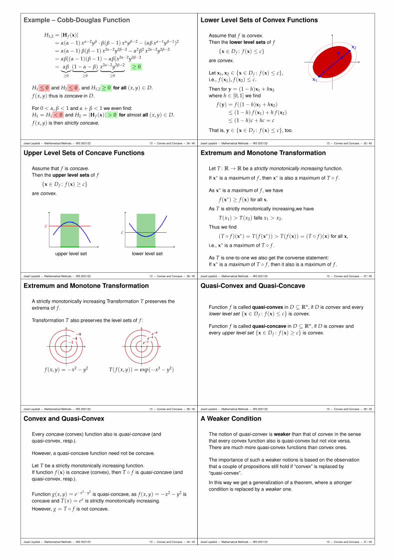
Example – Cobb-Douglas Function
H1,2 = |H f (x)|= α(α− 1) xα−2yβ · β(β− 1) xαyβ−2 − (αβ xα−1yβ−1)2
= α(α− 1) β(β− 1) x2α−2y2β−2 − α2β2 x2α−2y2β−2
= αβ[(α− 1)(β− 1)− αβ]x2α−2y2β−2
= αβ︸︷︷︸≥0
(1− α− β)︸ ︷︷ ︸≥0
x2α−2y2β−2︸ ︷︷ ︸
≥0
≥ 0
H1 ≤ 0 and H2 ≤ 0 , and H1,2 ≥ 0 for all (x, y) ∈ D.
f (x, y) thus is concave in D.
For 0 < α, β < 1 and α + β < 1 we even find:H1 = H1 < 0 and H2 = |H f (x)| > 0 for almost all (x, y) ∈ D.
f (x, y) is then strictly concave.
Josef Leydold – Mathematical Methods – WS 2021/22 13 – Convex and Concave – 34 / 45
Lower Level Sets of Convex Functions
Assume that f is convex.Then the lower level sets of f
x ∈ D f : f (x) ≤ care convex.
x1
x2y
Let x1, x2 ∈ x ∈ D f : f (x) ≤ c,i.e., f (x1), f (x2) ≤ c.
Then for y = (1− h)x1 + hx2where h ∈ [0, 1] we find
f (y) = f ((1− h)x1 + hx2)
≤ (1− h) f (x1) + h f (x2)
≤ (1− h)c + hc = c
That is, y ∈ x ∈ D f : f (x) ≤ c, too.
Josef Leydold – Mathematical Methods – WS 2021/22 13 – Convex and Concave – 35 / 45
Upper Level Sets of Concave Functions
Assume that f is concave.Then the upper level sets of f
x ∈ D f : f (x) ≥ care convex.
cc
upper level set lower level set
Josef Leydold – Mathematical Methods – WS 2021/22 13 – Convex and Concave – 36 / 45
Extremum and Monotone Transformation
Let T : R→ R be a strictly monotonically increasing function.
If x∗ is a maximum of f , then x∗ is also a maximum of T f .
As x∗ is a maximum of f , we have
f (x∗) ≥ f (x) for all x.
As T is strictly monotonically increasing,we have
T(x1) > T(x2) falls x1 > x2.
Thus we find
(T f )(x∗) = T( f (x∗)) > T( f (x)) = (T f )(x) for all x,
i.e., x∗ is a maximum of T f .
As T is one-to-one we also get the converse statement:If x∗ is a maximum of T f , then it also is a maximum of f .
Josef Leydold – Mathematical Methods – WS 2021/22 13 – Convex and Concave – 37 / 45
Extremum and Monotone Transformation
A strictly monotonically increasing Transformation T preserves theextrema of f .
Transformation T also preserves the level sets of f :
−1−4−9
−1−4−9
e−1e−4
e−9
e−1e−4
e−9
f (x, y) = −x2 − y2 T( f (x, y)) = exp(−x2 − y2)
Josef Leydold – Mathematical Methods – WS 2021/22 13 – Convex and Concave – 38 / 45
Quasi-Convex and Quasi-Concave
Function f is called quasi-convex in D ⊆ Rn, if D is convex and everylower level set x ∈ D f : f (x) ≤ c is convex.
Function f is called quasi-concave in D ⊆ Rn, if D is convex andevery upper level set x ∈ D f : f (x) ≥ c is convex.
Josef Leydold – Mathematical Methods – WS 2021/22 13 – Convex and Concave – 39 / 45
Convex and Quasi-Convex
Every concave (convex) function also is quasi-concave (andquasi-convex, resp.).
However, a quasi-concave function need not be concave.
Let T be a strictly monotonically increasing function.If function f (x) is concave (convex), then T f is quasi-concave (andquasi-convex, resp.).
Function g(x, y) = e−x2−y2is quasi-concave, as f (x, y) = −x2 − y2 is
concave and T(x) = ex is strictly monotonically increasing.
However, g = T f is not concave.
Josef Leydold – Mathematical Methods – WS 2021/22 13 – Convex and Concave – 40 / 45
A Weaker Condition
The notion of quasi-convex is weaker than that of convex in the sensethat every convex function also is quasi-convex but not vice versa.There are much more quasi-convex functions than convex ones.
The importance of such a weaker notions is based on the observationthat a couple of propositions still hold if “convex” is replaced by“quasi-convex”.
In this way we get a generalization of a theorem, where a strongercondition is replaced by a weaker one.
Josef Leydold – Mathematical Methods – WS 2021/22 13 – Convex and Concave – 41 / 45
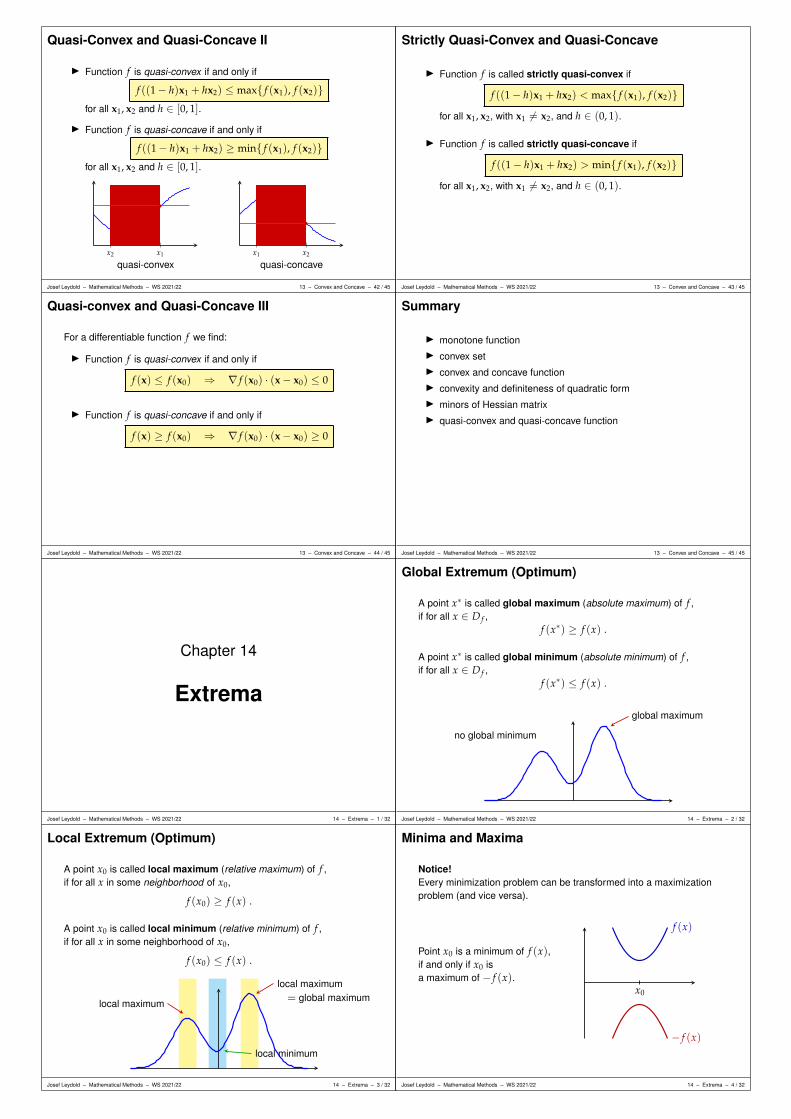
Quasi-Convex and Quasi-Concave II
I Function f is quasi-convex if and only if
f ((1− h)x1 + hx2) ≤ max f (x1), f (x2)for all x1, x2 and h ∈ [0, 1].
I Function f is quasi-concave if and only if
f ((1− h)x1 + hx2) ≥ min f (x1), f (x2)for all x1, x2 and h ∈ [0, 1].
x2 x1 x1 x2
quasi-convex quasi-concave
Josef Leydold – Mathematical Methods – WS 2021/22 13 – Convex and Concave – 42 / 45
Strictly Quasi-Convex and Quasi-Concave
I Function f is called strictly quasi-convex if
f ((1− h)x1 + hx2) < max f (x1), f (x2)for all x1, x2, with x1 6= x2, and h ∈ (0, 1).
I Function f is called strictly quasi-concave if
f ((1− h)x1 + hx2) > min f (x1), f (x2)for all x1, x2, with x1 6= x2, and h ∈ (0, 1).
Josef Leydold – Mathematical Methods – WS 2021/22 13 – Convex and Concave – 43 / 45
Quasi-convex and Quasi-Concave III
For a differentiable function f we find:
I Function f is quasi-convex if and only if
f (x) ≤ f (x0) ⇒ ∇ f (x0) · (x− x0) ≤ 0
I Function f is quasi-concave if and only if
f (x) ≥ f (x0) ⇒ ∇ f (x0) · (x− x0) ≥ 0
Josef Leydold – Mathematical Methods – WS 2021/22 13 – Convex and Concave – 44 / 45
Summary
I monotone functionI convex setI convex and concave functionI convexity and definiteness of quadratic formI minors of Hessian matrixI quasi-convex and quasi-concave function
Josef Leydold – Mathematical Methods – WS 2021/22 13 – Convex and Concave – 45 / 45
Chapter 14
Extrema
Josef Leydold – Mathematical Methods – WS 2021/22 14 – Extrema – 1 / 32
Global Extremum (Optimum)
A point x∗ is called global maximum (absolute maximum) of f ,if for all x ∈ D f ,
f (x∗) ≥ f (x) .
A point x∗ is called global minimum (absolute minimum) of f ,if for all x ∈ D f ,
f (x∗) ≤ f (x) .
global maximum
no global minimum
Josef Leydold – Mathematical Methods – WS 2021/22 14 – Extrema – 2 / 32
Local Extremum (Optimum)
A point x0 is called local maximum (relative maximum) of f ,if for all x in some neighborhood of x0,
f (x0) ≥ f (x) .
A point x0 is called local minimum (relative minimum) of f ,if for all x in some neighborhood of x0,
f (x0) ≤ f (x) .
local maximum= global maximumlocal maximum
local minimum
Josef Leydold – Mathematical Methods – WS 2021/22 14 – Extrema – 3 / 32
Minima and Maxima
Notice!Every minimization problem can be transformed into a maximizationproblem (and vice versa).
Point x0 is a minimum of f (x),if and only if x0 isa maximum of − f (x).
x0
f (x)
− f (x)
Josef Leydold – Mathematical Methods – WS 2021/22 14 – Extrema – 4 / 32

Critical Point
At a (local) maximum or minimum the first derivative of the functionmust vanish (i.e., must be equal to 0).
A point x0 is called a critical point (or stationary point) of functionf , if
f ′(x0) = 0
Necessary condition for differentiable functions:
Each extremum of f is a critical point of f .
Josef Leydold – Mathematical Methods – WS 2021/22 14 – Extrema – 5 / 32
Global Extremum
Sufficient condition:
Let x0 be a critical point of f .If f is concave, then x0 is a global maximum of f .If f is convex, then x0 is a global minimum of f .
If f is strictly concave (or convex), then the extremum is unique.
This condition immediately follows from the properties of (strictly)concave functions. Indeed, we have for all x 6= x0,
f (x)− f (x0) ≤ ∇ f (x0) · (x− x0) = 0 · (x− x0) = 0
and thusf (x0) ≥ f (x) .
Josef Leydold – Mathematical Methods – WS 2021/22 14 – Extrema – 6 / 32
Example – Global Extremum / Univariate∗
Let f (x) = ex − 2 x.
Function f is strictly convex:
f ′(x) = ex − 2f ′′(x) = ex > 0 for all x ∈ R
Critical point:
f ′(x) = ex − 2 = 0 ⇒ x0 = ln 2
x0 = ln 2 is the (unique) global minimum of f .
Josef Leydold – Mathematical Methods – WS 2021/22 14 – Extrema – 7 / 32
Example – Global Extremum / Multivariate
Let f : D = [0, ∞)2 → R, f (x, y) = 4 x14 y
14 − x− y
Hessian matrix at x:
H f (x) =
(− 3
4 x−74 y
14 1
4 x−34 y−
34
14 x−
34 y−
34 − 3
4 x14 y−
74
)
Leading principle minors:H1 = − 3
4 x−74 y
14 < 0
H2 = 12 x−
32 y−
32 > 0
f is strictly concave in D.
critical point: ∇ f = (x−34 y
14 − 1, x
14 y−
34 − 1) = 0
fx = x−34 y
14 − 1 = 0
fy = x14 y−
34 − 1 = 0
⇒ x0 = (1, 1)
x0 is the global maximum of f .
Josef Leydold – Mathematical Methods – WS 2021/22 14 – Extrema – 8 / 32
Sources of Errors
Find all global minima of f (x) =x3 + 2
3x.
x0
1. f ′(x) = 2(x3−1)3x2 ,
f ′′(x) = 2x3+43x3 .
2. critical point at x0 = 1.
3. f ′′(1) = 2 > 0⇒ global minimum ???
However, looking just at f ′′(1) is not sufficient as we are looking forglobal minima!
Beware! We have to look at f ′′(x) at all x ∈ D f .However, f ′′(−1) = − 2
3 < 0.Moreover, domain D = R \ 0 is not an interval.So f is not convex and we cannot apply our theorem.
Josef Leydold – Mathematical Methods – WS 2021/22 14 – Extrema – 9 / 32
Sources of Errors
Find all global maxima of f (x) = exp(−x2/2) .
x0
1. f ′(x) = x exp(−x2),
f ′′(x) = (x2 − 1) exp(−x2).
2. critical point at x0 = 0.
3. However,f ′′(0) = −1 < 0 but f ′′(2) = 2e−2 > 0.So f is not concave and thus there cannot be a global maximum.Really ???
Beware! We are checking a sufficient condition.Since an assumption does not hold ( f is not concave),we simply cannot apply the theorem.We cannot conclude that f does not have a global maximum.
Josef Leydold – Mathematical Methods – WS 2021/22 14 – Extrema – 10 / 32
Global Extrema in [a, b]∗
Extrema of f (x) in closed interval [a, b].
Procedure for differentiable functions:
(1) Compute f ′(x).
(2) Find all stationary points xi (i.e., f ′(xi) = 0).
(3) Evaluate f (x) for all candidates:I all stationary points xi,I boundary points a and b.
(4) Largest of these values is global maximum,smallest of these values is global minimum.
It is not necessary to compute f ′′(xi).
Josef Leydold – Mathematical Methods – WS 2021/22 14 – Extrema – 11 / 32
Global Extrema in [a, b]∗
Find all global extrema of function
f : [0,5; 8,5]→ R, x 7→ 112
x3 − x2 + 3 x + 1
(1) f ′(x) = 14 x2 − 2 x + 3.
(2) 14 x2 − 2 x + 3 = 0 has roots x1 = 2 and x2 = 6.
(3) f (0.5) = 2.260f (2) = 3.667f (6) = 1.000 ⇒ global minimum
f (8.5) = 5.427 ⇒ global maximum
(4) x2 = 6 is the global minimum andb = 8.5 is the global maximum of f .
Josef Leydold – Mathematical Methods – WS 2021/22 14 – Extrema – 12 / 32

Global Extrema in (a, b)∗
Extrema of f (x) in open interval (a, b) (or (−∞, ∞)).
Procedure for differentiable functions:
(1) Compute f ′(x).
(2) Find all stationary points xi (i.e., f ′(xi) = 0).
(3) Evaluate f (x) for all stationary points xi.
(4) Determine limx→a f (x) and limx→b f (x).
(5) Largest of these values is global maximum,smallest of these values is global minimum.
(6) A global extremum exists only if the largest (smallest) valueis obtained in a stationary point !
Josef Leydold – Mathematical Methods – WS 2021/22 14 – Extrema – 13 / 32
Global Extrema in (a, b)∗
Compute all global extrema of
f : R→ R, x 7→ e−x2
(1) f ′(x) = −2x e−x2.
(2) f ′(x) = −2x e−x2= 0 has unique root x1 = 0.
(3) f (0) = 1 ⇒ global maximum
limx→−∞ f (x) = 0 ⇒ no global minimum
limx→∞ f (x) = 0
(4) The function has a global maximum in x1 = 0,but no global minimum.
Josef Leydold – Mathematical Methods – WS 2021/22 14 – Extrema – 14 / 32
Existence and Uniqueness
I A function need not have maxima or minima:
f : (0, 1)→ R, x 7→ x
(Points 0 and 1 are not in domain (0, 1).)
I (Global) maxima need not be unique:
f : R→ R, x 7→ x4 − 2 x2
has two global minima at −1 and 1.
Josef Leydold – Mathematical Methods – WS 2021/22 14 – Extrema – 15 / 32
Example – Local Extrema
-2 -1 0 1 2 -2-1
01
2
-1
0
1
f (x, y) =16
x3 − x +14
x y2
Josef Leydold – Mathematical Methods – WS 2021/22 14 – Extrema – 16 / 32
Local Extremum
A point x0 is a local maximum (or local minimum) of f , ifI x0 is a critical point of f ,I f is locally concave (and locally convex, resp.) around x0.
Sufficient condition for two times differentiable functions:
Let x0 be a critical point of f . Then
I f ′′(x0) negative definite ⇒ x0 is local maximum
I f ′′(x0) positive definite ⇒ x0 is local minimum
It is sufficient to evaluate f ′′(x) at the critical point x0.(In opposition to the condition for global extrema.)
Josef Leydold – Mathematical Methods – WS 2021/22 14 – Extrema – 17 / 32
Necessary and Sufficient
We again want to explain two important concepts using the example oflocal minima.
Condition “ f ′(x0) = 0” is necessary for a local minimum:
Every local minimum must have this properties.However, not every point with such a property is a local minimum(e.g. x0 = 0 in f (x) = x3).Stationary points are candidates for local extrema.
Condition “ f ′(x0) = 0 and f ′′(x0) is positive definite” is sufficient for alocal minimum.
If it is satisfied, then x0 is a local minimum.However, there are local minima where this condition does not hold(e.g. x0 = 0 in f (x) = x4).If it is not satisfied, we cannot draw any conclusion.
Josef Leydold – Mathematical Methods – WS 2021/22 14 – Extrema – 18 / 32
Procedure – Univariate Functions∗
Sufficient conditionfor local extrema of a differentiable function in one variable:
1. Compute f ′(x) and f ′′(x).
2. Find all roots xi of f ′(xi) = 0 (critical points).
3. If f ′′(xi) < 0 ⇒ xi is a local maximum.
If f ′′(xi) > 0 ⇒ xi is a local minimum.
If f ′′(xi) = 0 ⇒ no conclusion possible!
If f ′′(xi) = 0 we need more sophisticated methods!(E.g., terms of higher order of the Taylor series expansion around xi.)
Josef Leydold – Mathematical Methods – WS 2021/22 14 – Extrema – 19 / 32
Example – Local Extrema∗
Find all local extrema of
f (x) =112
x3 − x2 + 3 x + 1
x1 x2
1. f ′(x) = 14 x2 − 2 x + 3,
f ′′(x) = 12 x− 2.
2. 14 x2 − 2 x + 3 = 0has roots
x1 = 2 and x2 = 6.
3. f ′′(2) = −1 ⇒ x1 is a local maximum.
f ′′(6) = 1 ⇒ x2 is a local minimum.
Josef Leydold – Mathematical Methods – WS 2021/22 14 – Extrema – 20 / 32
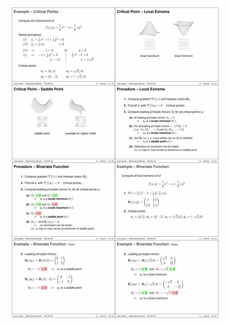
Example – Critical Points
Compute all critical points of
f (x, y) =16
x3 − x +14
x y2
Partial derivatives:
(I) fx = 12 x2 − 1 + 1
4 y2 = 0(I I) fy = 1
2 x y = 0
(I I) ⇒ x = 0 or y = 0(I) ⇒ −1 + 1
4 y2 = 0y = ±2
12 x2 − 1 = 0
x = ±√
2
Critical points:
x1 = (0, 2) x3 = (√
2, 0)
x2 = (0, −2) x4 = (−√
2, 0)
Josef Leydold – Mathematical Methods – WS 2021/22 14 – Extrema – 21 / 32
Critical Point – Local Extrema
local maximum local minimum
Josef Leydold – Mathematical Methods – WS 2021/22 14 – Extrema – 22 / 32
Critical Point – Saddle Point
saddle point example for higher order
Josef Leydold – Mathematical Methods – WS 2021/22 14 – Extrema – 23 / 32
Procedure – Local Extrema
1. Compute gradient ∇ f (x) and Hessian matrix H f .
2. Find all xi with ∇ f (xi) = 0 (critical points).
3. Compute leading principle minors Hk for all critical points xi:
(a) All leading principle minors Hk > 0⇒ x0 is a locale minimum of f .
(b) For all leading principle minors, (−1)k Hk > 0[ i.e., H1, H3, . . . < 0 and H2, H4, . . . > 0 ]⇒ x0 is a locale maximum of f .
(c) det(H f (xi)) 6= 0 but neither (a) nor (b) is satisfied⇒ x0 is a saddle point of f .
(d) Otherwise no conclusion can be drawn,i.e., xi may or may not be an extremum or saddle point.
Josef Leydold – Mathematical Methods – WS 2021/22 14 – Extrema – 24 / 32
Procedure – Bivariate Function
1. Compute gradient ∇ f (x) and Hessian matrix H f .
2. Find all xi with ∇ f (xi) = 0 (critical points).
3. Compute leading principle minors Hk for all critical points xi:
(a) H2 > 0 and H1 > 0⇒ x0 is a locale minimum of f .
(b) H2 > 0 and H1 < 0⇒ x0 is a locale maximum of f .
(c) H2 < 0⇒ x0 is a saddle point of f .
(d) H2 = det(H f (x0)) = 0⇒ no conclusion can be drawn,
i.e., xi may or may not be an extremum or saddle point.
Josef Leydold – Mathematical Methods – WS 2021/22 14 – Extrema – 25 / 32
Example – Bivariate Function
Compute all local extrema of of
f (x, y) =16
x3 − x +14
x y2
1. ∇ f = ( 12 x2 − 1 + 1
4 y2, 12 x y)
H f (x, y) =
(x 1
2 y12 y 1
2 x
)
2. Critical points:
x1 = (0, 2), x2 = (0,−2), x3 = (√
2, 0), x4 = (−√
2, 0)
Josef Leydold – Mathematical Methods – WS 2021/22 14 – Extrema – 26 / 32
Example – Bivariate Function / Cont.
3. Leading principle minors:
H f (x1) = H f (0, 2) =
(0 11 0
)
H2 = −1 < 0 ⇒ x1 is a saddle point
H f (x2) = H f (0,−2) =
(0 −1−1 0
)
H2 = −1 < 0 ⇒ x2 is a saddle point
Josef Leydold – Mathematical Methods – WS 2021/22 14 – Extrema – 26 / 32
Example – Bivariate Function / Cont.
3. Leading principle minors:
H f (x3) = H f (√
2, 0) =
(√2 0
0√
22
)
H2 = 1 > 0 and H1 =√
2 > 0
⇒ x3 is a local minimum
H f (x4) = H f (−√
2, 0) =
(−√
2 0
0 −√
22
)
H2 = 1 > 0 and H1 = −√
2 < 0
⇒ x4 is a local maximum
Josef Leydold – Mathematical Methods – WS 2021/22 14 – Extrema – 26 / 32

Derivative of Optimal Value
Let p, r > 0 and f : D = [0, ∞)2 → R, f (x, y) = 4 x14 y
14 − px− ry
Hessian matrix: H f (x) =
(− 3
4 x−74 y
14 1
4 x−34 y−
34
14 x−
34 y−
34 − 3
4 x14 y−
74
)
Leading principle minors:H1 = − 3
4 x−74 y
14 < 0
H2 = 12 x−
32 y−
32 > 0
f is strictly concave in D.
Critical point: ∇ f = (x−34 y
14 − p, x
14 y−
34 − r) = 0
fx = x−34 y
14 − p = 0
fy = x14 y−
34 − r = 0
⇒ x0 =(√
1r p3 ,
√1
r3 p
)
x0 is the global maximum of f .
Question:What is the derivative of optimal value f ∗ = f (x0) w.r.t. r or p?
Josef Leydold – Mathematical Methods – WS 2021/22 14 – Extrema – 27 / 32
Envelope Theorem
We are given functionx 7→ f (x, r)
x = (x1, . . . , xn) . . . variable (endogeneous)
r = (r1, . . . , rk) . . . parameter (exogeneous)with extremum x∗.
This extremum depends on parameter r:
x∗ = x∗(r)
and so does the optimal value f ∗:
f ∗(r) = f (x∗(r), r)
We have:∂ f ∗(r)
∂rj=
∂ f (x, r)∂rj
∣∣∣∣x=x∗(r)
Josef Leydold – Mathematical Methods – WS 2021/22 14 – Extrema – 28 / 32
Envelope Theorem / Proof Idea
∂ f ∗(r)∂rj
=∂ f (x∗(r), r)
∂rj
∣∣∣∣x=x∗(r)
[ chain rule ]
=n
∑i=1
fxi(x∗(r), r)
︸ ︷︷ ︸= 0
as x∗ is a critical point
·∂x∗i (r)∂rj
+∂ f (x, r)
∂rj
∣∣∣∣x=x∗(r)
=∂ f (x, r)
∂rj
∣∣∣∣x=x∗(r)
Josef Leydold – Mathematical Methods – WS 2021/22 14 – Extrema – 29 / 32
Example – Envelope Theorem
The (unique) maximum of
f : D = [0, ∞)2 → R, f (x, y) = 4 x14 y
14 − px− ry
is x∗(p, r) = (x∗(p, r), y∗(p, r)) =(√
1r p3 ,
√1
r3 p
).
Question:What is the derivative of optimal value f ∗ = f (x0) w.r.t. r or p?
∂ f ∗(p, r)∂p
=∂ f (x; p, r)
∂p
∣∣∣∣x=x∗(p,r)
= −x∣∣∣x=x∗(p,r)
= −√
1r p3
∂ f ∗(p, r)∂r
=∂ f (x; p, r)
∂r
∣∣∣∣x=x∗(p,r)
= −y∣∣∣x=x∗(p,r)
= −√
1r3 p
Josef Leydold – Mathematical Methods – WS 2021/22 14 – Extrema – 30 / 32
A Geometric Interpretation
Let f (x, r) =√
x− rx. We want f ∗(r) = maxx f (x, r).
Graphs of gx(r) = f (x, r) for various values of x.
r
g4/11g1/2
g2/3
g1
g3/2f ∗(r)
Josef Leydold – Mathematical Methods – WS 2021/22 14 – Extrema – 31 / 32
Summary
I global extremumI local extremumI minimum, maximum and saddle pointI critical pointI hessian matrix and principle minorsI envelope theorem
Josef Leydold – Mathematical Methods – WS 2021/22 14 – Extrema – 32 / 32
Chapter 15
Lagrange Function
Josef Leydold – Mathematical Methods – WS 2021/22 15 – Lagrange Function – 1 / 28
Constraint Optimization
Find the extrema of function
f (x, y)
subject tog(x, y) = c
Example:Find the extrema of function
f (x, y) = x2 + 2 y2
subject tog(x, y) = x + y = 3
Josef Leydold – Mathematical Methods – WS 2021/22 15 – Lagrange Function – 2 / 28

Graphical Solution
For the case of two variables we can find a solution graphically.
1. Draw the constraint g(x, y) = c in the xy-plain.(The feasible region is a curve in the plane)
2. Draw appropriate contour lines of objective function f (x, y).
3. Investigate which contour lines of the objective function intersectwith the feasible region.Estimate the (approximate) location of the extrema.
Josef Leydold – Mathematical Methods – WS 2021/22 15 – Lagrange Function – 3 / 28
Example – Graphical Solution
1
2x + y = 3
∇g
∇ f ∇ f = λ∇g
minimum in (2, 1)
Extrema of f (x, y) = x2 + 2 y2 subject to g(x, y) = x + y = 3
Josef Leydold – Mathematical Methods – WS 2021/22 15 – Lagrange Function – 4 / 28
Lagrange Approach
Let x∗ be an extremum of f (x, y) subject to g(x, y) = c.Then ∇ f (x∗) and ∇g(x∗) are proportional, i.e.,
∇ f (x∗) = λ∇g(x∗)
where λ is some proportionality factor.
fx(x∗) = λ gx(x∗)fy(x∗) = λ gy(x∗)g(x∗) = c
∇g
∇ f
x∗
Transformation yields
fx(x∗)− λ gx(x∗) = 0fy(x∗)− λ gy(x∗) = 0c− g(x∗) = 0
The l.h.s. is the gradient of L(x, y; λ) = f (x, y) + λ (c− g(x, y)) .
Josef Leydold – Mathematical Methods – WS 2021/22 15 – Lagrange Function – 5 / 28
Lagrange Function
We create a new function from f , g and an auxiliary variable λ,called Lagrange function:
L(x, y; λ) = f (x, y) + λ (c− g(x, y))
Auxiliary variable λ is called Lagrange multiplier.
Local extrema of f subject to g(x, y) = c are critical points ofLagrange function L:
Lx = fx − λ gx = 0Ly = fy − λ gy = 0Lλ = c− g(x, y) = 0
Josef Leydold – Mathematical Methods – WS 2021/22 15 – Lagrange Function – 6 / 28
Example – Lagrange Function
Compute the local extrema of
f (x, y) = x2 + 2y2 subject to g(x, y) = x + y = 3
Lagrange function:
L(x, y, λ) = (x2 + 2y2) + λ(3− (x + y))
Critical points:Lx = 2x− λ = 0Ly = 4y− λ = 0Lλ = 3− x− y = 0
⇒ unique critical point: (x0; λ0) = (2, 1; 4)
Josef Leydold – Mathematical Methods – WS 2021/22 15 – Lagrange Function – 7 / 28
Bordered Hessian Matrix
Matrix
H(x; λ) =
0 gx gy
gx Lxx Lxy
gy Lyx Lyy
is called the bordered Hessian Matrix.
Sufficient condition for local extremum:
Let (x0; λ0) be a critical point of L.I |H(x0; λ0)| > 0 ⇒ x0 is a local maximumI |H(x0; λ0)| < 0 ⇒ x0 is a local minimumI |H(x0; λ0)| = 0 ⇒ no conclusion possible
Josef Leydold – Mathematical Methods – WS 2021/22 15 – Lagrange Function – 8 / 28
Example – Bordered Hessian Matrix
Compute the local extrema of
f (x, y) = x2 + 2y2 subject to g(x, y) = x + y = 3
Lagrange function: L(x, y, λ) = (x2 + 2y2) + λ(3− x− y)Critical point: (x0; λ0) = (2, 1; 4)
Determinant of the bordered Hessian:
|H(x0; λ0)| =
∣∣∣∣∣∣∣
0 gx gy
gx Lxx Lxy
gy Lyx Lyy
∣∣∣∣∣∣∣=
∣∣∣∣∣∣∣
0 1 11 2 01 0 4
∣∣∣∣∣∣∣= −6 < 0
⇒ x0 = (2, 1) is a local minimum.
Josef Leydold – Mathematical Methods – WS 2021/22 15 – Lagrange Function – 9 / 28
Many Variables and Constraints
Objective function
f (x1, . . . , xn)
and constraintsg1(x1, . . . , xn) = c1
...
gk(x1, . . . , xn) = ck
(k < n)
Optimization problem: min / max f (x) subject to g(x) = c.
Lagrange Function:
L(x; λ) = f (x) + λT(c− g(x))
Josef Leydold – Mathematical Methods – WS 2021/22 15 – Lagrange Function – 10 / 28
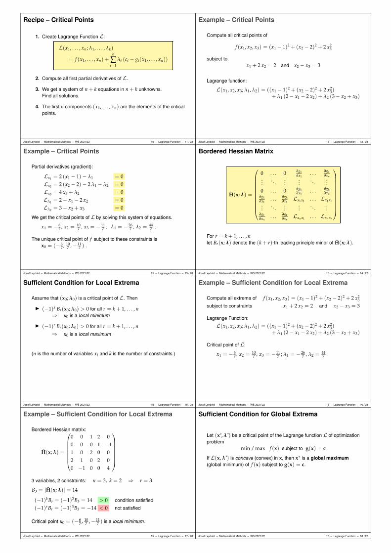
Recipe – Critical Points
1. Create Lagrange Function L:
L(x1, . . . , xn; λ1, . . . , λk)
= f (x1, . . . , xn) +k
∑i=1
λi (ci − gi(x1, . . . , xn))
2. Compute all first partial derivatives of L.
3. We get a system of n + k equations in n + k unknowns.Find all solutions.
4. The first n components (x1, . . . , xn) are the elements of the criticalpoints.
Josef Leydold – Mathematical Methods – WS 2021/22 15 – Lagrange Function – 11 / 28
Example – Critical Points
Compute all critical points of
f (x1, x2, x3) = (x1 − 1)2 + (x2 − 2)2 + 2 x23
subject tox1 + 2 x2 = 2 and x2 − x3 = 3
Lagrange function:
L(x1, x2, x3; λ1, λ2) = ((x1 − 1)2 + (x2 − 2)2 + 2 x23)
+ λ1 (2− x1 − 2 x2) + λ2 (3− x2 + x3)
Josef Leydold – Mathematical Methods – WS 2021/22 15 – Lagrange Function – 12 / 28
Example – Critical Points
Partial derivatives (gradient):
Lx1 = 2 (x1 − 1)− λ1 = 0Lx2 = 2 (x2 − 2)− 2 λ1 − λ2 = 0Lx3 = 4 x3 + λ2 = 0Lλ1 = 2− x1 − 2 x2 = 0Lλ2 = 3− x2 + x3 = 0
We get the critical points of L by solving this system of equations.
x1 = − 67 , x2 = 10
7 , x3 = − 117 ; λ1 = − 26
7 , λ2 = 447 .
The unique critical point of f subject to these constraints isx0 = (− 6
7 , 107 ,− 11
7 ) .
Josef Leydold – Mathematical Methods – WS 2021/22 15 – Lagrange Function – 13 / 28
Bordered Hessian Matrix
H(x; λ) =
0 . . . 0 ∂g1∂x1
. . . ∂g1∂xn
.... . .
......
. . ....
0 . . . 0 ∂gk∂x1
. . . ∂gk∂xn
∂g1∂x1
. . . ∂gk∂x1
Lx1x1 . . . Lx1xn
.... . .
......
. . ....
∂g1∂xn
. . . ∂gk∂xn
Lxnx1 . . . Lxnxn
For r = k + 1, . . . , nlet Br(x; λ) denote the (k + r)-th leading principle minor of H(x; λ).
Josef Leydold – Mathematical Methods – WS 2021/22 15 – Lagrange Function – 14 / 28
Sufficient Condition for Local Extrema
Assume that (x0; λ0) is a critical point of L. Then
I (−1)k Br(x0; λ0) > 0 for all r = k + 1, . . . , n⇒ x0 is a local minimum
I (−1)r Br(x0; λ0) > 0 for all r = k + 1, . . . , n⇒ x0 is a local maximum
(n is the number of variables xi and k is the number of constraints.)
Josef Leydold – Mathematical Methods – WS 2021/22 15 – Lagrange Function – 15 / 28
Example – Sufficient Condition for Local Extrema
Compute all extrema of f (x1, x2, x3) = (x1 − 1)2 + (x2 − 2)2 + 2 x23
subject to constraints x1 + 2 x2 = 2 and x2 − x3 = 3
Lagrange Function:
L(x1, x2, x3; λ1, λ2) = ((x1 − 1)2 + (x2 − 2)2 + 2 x23)
+ λ1 (2− x1 − 2 x2) + λ2 (3− x2 + x3)
Critical point of L:
x1 = − 67 , x2 = 10
7 , x3 = − 117 ; λ1 = − 26
7 , λ2 = 447 .
Josef Leydold – Mathematical Methods – WS 2021/22 15 – Lagrange Function – 16 / 28
Example – Sufficient Condition for Local Extrema
Bordered Hessian matrix:
H(x; λ) =
0 0 1 2 00 0 0 1 −11 0 2 0 02 1 0 2 00 −1 0 0 4
3 variables, 2 constraints: n = 3, k = 2 ⇒ r = 3
B3 = |H(x; λ)| = 14
(−1)kBr = (−1)2B3 = 14 > 0 condition satisfied
(−1)rBr = (−1)3B3 = −14 < 0 not satisfied
Critical point x0 = (− 67 , 10
7 ,− 117 ) is a local minimum.
Josef Leydold – Mathematical Methods – WS 2021/22 15 – Lagrange Function – 17 / 28
Sufficient Condition for Global Extrema
Let (x∗, λ∗) be a critical point of the Lagrange function L of optimizationproblem
min / max f (x) subject to g(x) = c
If L(x, λ∗) is concave (convex) in x, then x∗ is a global maximum(global minimum) of f (x) subject to g(x) = c.
Josef Leydold – Mathematical Methods – WS 2021/22 15 – Lagrange Function – 18 / 28

Example – Sufficient Condition for Global Extrema
(x∗, y∗; λ∗) = (2, 1; 4) is a critical point of the Lagrange function L ofoptimization problem
min / max f (x, y) = x2 + 2y2 subject to g(x, y) = x + y = 3
Lagrange function:
L(x, y, λ∗) = (x2 + 2y2) + 4 · (3− (x + y))
Hessian matrix:
HL(x, y) =
(2 00 4
)H1 = 2 > 0H2 = 8 > 0
L is convex in (x, y).
Thus (x∗, y∗) = (2, 1) is a global minimum.
Josef Leydold – Mathematical Methods – WS 2021/22 15 – Lagrange Function – 19 / 28
Example – Sufficient Condition for Global Extrema
(x∗; λ∗) = (− 67 , 10
7 ,− 117 ;− 26
7 , 447 )
is a critical point of the Lagrange function of optimization problem
min / max f (x1, x2, x3) = (x1 − 1)2 + (x2 − 2)2 + 2 x23
subject to g1(x1, x2, x3) = x1 + 2 x2 = 2g2(x1, x2, x3) = x2 − x3 = 3
Lagrange function:
L(x; λ∗) = ((x1 − 1)2 + (x2 − 2)2 + 2 x23)
− 267 (2− x1 − 2 x2) +
447 (3− x2 + x3)
Josef Leydold – Mathematical Methods – WS 2021/22 15 – Lagrange Function – 20 / 28
Example – Sufficient Condition for Global Extrema
Hessian matrix:
HL(x1, x2, x3) =
2 0 00 2 00 0 4
H1 = 2 > 0H2 = 4 > 0H3 = 16 > 0
L is convex in x.
x∗= (− 67 , 10
7 ,− 117 ) is a global minimum.
Josef Leydold – Mathematical Methods – WS 2021/22 15 – Lagrange Function – 21 / 28
Interpretation of Lagrange Multiplier
Extremum x∗ of optimization problem
min / max f (x) subject to g(x) = c
depends on c, x∗= x∗(c), and so does the extremal value
f ∗(c) = f (x∗(c))
How does f ∗(c) change with varying c?
∂ f ∗
∂cj(c) = λ∗j(c)
That is, Lagrange multiplier λj is the derivative of the extremal valuew.r.t. exogeneous variable cj in constraint gj(x) = cj.
Josef Leydold – Mathematical Methods – WS 2021/22 15 – Lagrange Function – 22 / 28
Proof Idea
Lagrange function L and objective function f coincide in extemum x∗.
∂ f ∗(c)∂cj
=∂L(x∗(c), λ(c))
∂cj[ chain rule ]
=n
∑i=1Lxi(x
∗(c), λ(c))︸ ︷︷ ︸
= 0as x∗ is a critical point
·∂x∗i (c)∂cj
+∂L(x, c)
∂cj
∣∣∣∣(x∗(c),λ∗(c))
=∂L(x, c)
∂cj
∣∣∣∣(x∗(c),λ∗(c))
=∂
∂cj
(f (x) +
k
∑i=1
λi(ci − gi(x)))∣∣∣∣∣
(x∗(c),λ∗(c))
= λ∗j(c)
Josef Leydold – Mathematical Methods – WS 2021/22 15 – Lagrange Function – 23 / 28
Example – Lagrange Multiplier
(x∗, y∗) = (2, 1) is a minimum of optimization problem
min / max f (x, y) = x2 + 2y2
subject to g(x, y) = x + y = c = 3
with λ∗ = 4.
How does the minimal value f ∗(c) change with varying c?
d f ∗
dc= λ∗= 4
Josef Leydold – Mathematical Methods – WS 2021/22 15 – Lagrange Function – 24 / 28
Envelope Theorem
What is the derivative of the extremal value f ∗of optimization problem
min / max f (x, p) subject to g(x, p) = c
w.r.t. parameters (exogeneous variables) p?
∂ f ∗(p)∂pj
=∂L(x, p)
∂pj
∣∣∣∣(x∗(p),λ∗(p))
Josef Leydold – Mathematical Methods – WS 2021/22 15 – Lagrange Function – 25 / 28
Example – Roy’s Identity
Maximize utility function
max U(x) subject to pT · x = w
The maximal utility depends on prices p and income w ab:
U∗= U∗(p, w) [ indirect utility function ]
Lagrange function L(x, λ) = U(x) + λ (w− pT · x)
∂U∗
∂pj=
∂L∂pj
= −λ∗x∗j and∂U∗
∂w=
∂L∂w
= λ∗
and thus
x∗j = −∂U∗/∂pj
∂U∗/∂w[ Marshallian demand function ]
Josef Leydold – Mathematical Methods – WS 2021/22 15 – Lagrange Function – 26 / 28
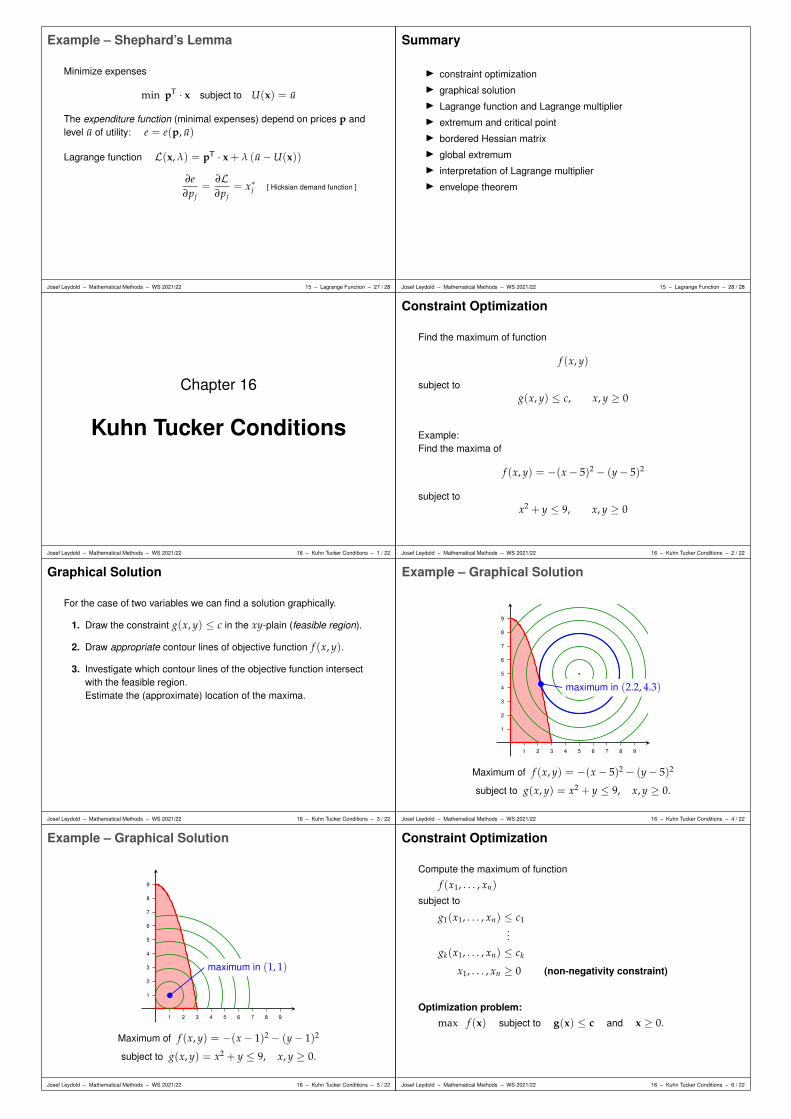
Example – Shephard’s Lemma
Minimize expenses
min pT · x subject to U(x) = u
The expenditure function (minimal expenses) depend on prices p andlevel u of utility: e = e(p, u)
Lagrange function L(x, λ) = pT · x + λ (u−U(x))
∂e∂pj
=∂L∂pj
= x∗j [ Hicksian demand function ]
Josef Leydold – Mathematical Methods – WS 2021/22 15 – Lagrange Function – 27 / 28
Summary
I constraint optimizationI graphical solutionI Lagrange function and Lagrange multiplierI extremum and critical pointI bordered Hessian matrixI global extremumI interpretation of Lagrange multiplierI envelope theorem
Josef Leydold – Mathematical Methods – WS 2021/22 15 – Lagrange Function – 28 / 28
Chapter 16
Kuhn Tucker Conditions
Josef Leydold – Mathematical Methods – WS 2021/22 16 – Kuhn Tucker Conditions – 1 / 22
Constraint Optimization
Find the maximum of function
f (x, y)
subject tog(x, y) ≤ c, x, y ≥ 0
Example:Find the maxima of
f (x, y) = −(x− 5)2 − (y− 5)2
subject tox2 + y ≤ 9, x, y ≥ 0
Josef Leydold – Mathematical Methods – WS 2021/22 16 – Kuhn Tucker Conditions – 2 / 22
Graphical Solution
For the case of two variables we can find a solution graphically.
1. Draw the constraint g(x, y) ≤ c in the xy-plain (feasible region).
2. Draw appropriate contour lines of objective function f (x, y).
3. Investigate which contour lines of the objective function intersectwith the feasible region.Estimate the (approximate) location of the maxima.
Josef Leydold – Mathematical Methods – WS 2021/22 16 – Kuhn Tucker Conditions – 3 / 22
Example – Graphical Solution
1 2 3 4 5 6 7 8 9
1
2
3
4
5
6
7
8
9
maximum in (2.2, 4.3)
Maximum of f (x, y) = −(x− 5)2 − (y− 5)2
subject to g(x, y) = x2 + y ≤ 9, x, y ≥ 0.
Josef Leydold – Mathematical Methods – WS 2021/22 16 – Kuhn Tucker Conditions – 4 / 22
Example – Graphical Solution
1 2 3 4 5 6 7 8 9
1
2
3
4
5
6
7
8
9
maximum in (1, 1)
Maximum of f (x, y) = −(x− 1)2 − (y− 1)2
subject to g(x, y) = x2 + y ≤ 9, x, y ≥ 0.
Josef Leydold – Mathematical Methods – WS 2021/22 16 – Kuhn Tucker Conditions – 5 / 22
Constraint Optimization
Compute the maximum of function
f (x1, . . . , xn)
subject to
g1(x1, . . . , xn) ≤ c1...
gk(x1, . . . , xn) ≤ ck
x1, . . . , xn ≥ 0 (non-negativity constraint)
Optimization problem:
max f (x) subject to g(x) ≤ c and x ≥ 0.
Josef Leydold – Mathematical Methods – WS 2021/22 16 – Kuhn Tucker Conditions – 6 / 22
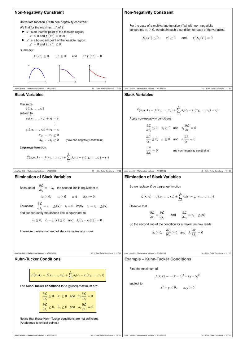
Non-Negativity Constraint
Univariate function f with non-negativity constraint.
We find for the maximum x∗ of f :I x∗ is an interior point of the feasible region:
x∗ > 0 and f ′(x∗) = 0; orI x∗ is a boundary point of the feasible region:
x∗ = 0 and f ′(x∗) ≤ 0.
Summary:
f ′(x∗) ≤ 0, x∗ ≥ 0 and x∗ f ′(x∗) = 0
Josef Leydold – Mathematical Methods – WS 2021/22 16 – Kuhn Tucker Conditions – 7 / 22
Non-Negativity Constraint
For the case of a multivariate function f (x) with non-negativityconstraints xj ≥ 0, we obtain such a condition for each of the variables:
fxj(x∗) ≤ 0, x∗j ≥ 0 and x∗j fxj(x
∗) = 0
Josef Leydold – Mathematical Methods – WS 2021/22 16 – Kuhn Tucker Conditions – 8 / 22
Slack Variables
Maximizef (x1, . . . , xn)
subject to
g1(x1, . . . , xn) + s1 = c1...
gk(x1, . . . , xn) + sk = ck
x1, . . . , xn ≥ 0s1, . . . , sk ≥ 0 (new non-negativity constraint)
Lagrange function:
L(x, s, λ) = f (x1, . . . , xn) +k
∑i=1
λi(ci − gi(x1, . . . , xn)− si)
Josef Leydold – Mathematical Methods – WS 2021/22 16 – Kuhn Tucker Conditions – 9 / 22
Slack Variables
L(x, s, λ) = f (x1, . . . , xn) +k
∑i=1
λi(ci − gi(x1, . . . , xn)− si)
Apply non-negativity conditions:
∂L∂xj≤ 0, xj ≥ 0 and xj
∂L∂xj
= 0
∂L∂si≤ 0, si ≥ 0 and si
∂L∂si
= 0
∂L∂λi
= 0 (no non-negativity constraint)
Josef Leydold – Mathematical Methods – WS 2021/22 16 – Kuhn Tucker Conditions – 10 / 22
Elimination of Slack Variables
Because of∂L∂si
= −λi the second line is equivalent to
λi ≥ 0, si ≥ 0 and λisi = 0
Equations∂L∂λi
= ci − gi(x)− si = 0 imply si = ci − gi(x)
and consequently the second line is equivalent to
λi ≥ 0, ci − gi(x) ≥ 0 and λi(ci − gi(x)) = 0 .
Therefore there is no need of slack variables any more.
Josef Leydold – Mathematical Methods – WS 2021/22 16 – Kuhn Tucker Conditions – 11 / 22
Elimination of Slack Variables
So we replace L by Lagrange function
L(x, λ) = f (x1, . . . , xn) +k
∑i=1
λi(ci − gi(x1, . . . , xn))
Observe that
∂L∂xj
=∂L∂xj
and∂L∂λi
= ci − gi(x)
So the second line of the condition for a maximum now reads
λi ≥ 0,∂L∂λi≥ 0 and λi
∂L∂λi
= 0
Josef Leydold – Mathematical Methods – WS 2021/22 16 – Kuhn Tucker Conditions – 12 / 22
Kuhn-Tucker Conditions
L(x, λ) = f (x1, . . . , xn) +k
∑i=1
λi(ci − gi(x1, . . . , xn))
The Kuhn-Tucker conditions for a (global) maximum are:
∂L∂xj≤ 0, xj ≥ 0 and xj
∂L∂xj
= 0
∂L∂λi≥ 0, λi ≥ 0 and λi
∂L∂λi
= 0
Notice that these Kuhn-Tucker conditions are not sufficient.(Analogous to critical points.)
Josef Leydold – Mathematical Methods – WS 2021/22 16 – Kuhn Tucker Conditions – 13 / 22
Example – Kuhn-Tucker Conditions
Find the maximum of
f (x, y) = −(x− 5)2 − (y− 5)2
subject tox2 + y ≤ 9, x, y ≥ 0
Lagrange function:
L(x, y; λ) = −(x− 5)2 − (y− 5)2 + λ(9− x2 − y)
Josef Leydold – Mathematical Methods – WS 2021/22 16 – Kuhn Tucker Conditions – 14 / 22
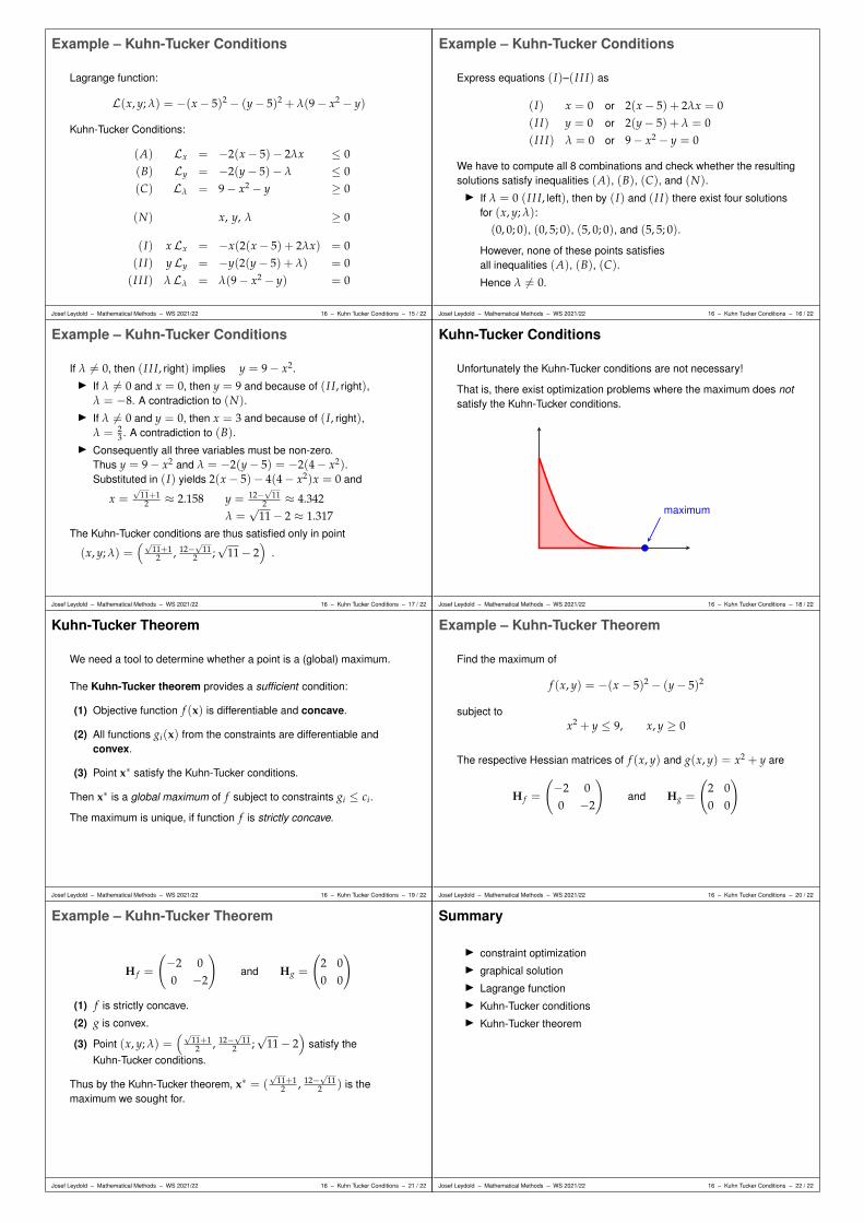
Example – Kuhn-Tucker Conditions
Lagrange function:
L(x, y; λ) = −(x− 5)2 − (y− 5)2 + λ(9− x2 − y)
Kuhn-Tucker Conditions:
(A) Lx = −2(x− 5)− 2λx ≤ 0(B) Ly = −2(y− 5)− λ ≤ 0(C) Lλ = 9− x2 − y ≥ 0
(N) x, y, λ ≥ 0
(I) xLx = −x(2(x− 5) + 2λx) = 0(I I) yLy = −y(2(y− 5) + λ) = 0(I I I) λLλ = λ(9− x2 − y) = 0
Josef Leydold – Mathematical Methods – WS 2021/22 16 – Kuhn Tucker Conditions – 15 / 22
Example – Kuhn-Tucker Conditions
Express equations (I)–(I I I) as
(I) x = 0 or 2(x− 5) + 2λx = 0(I I) y = 0 or 2(y− 5) + λ = 0(I I I) λ = 0 or 9− x2 − y = 0
We have to compute all 8 combinations and check whether the resultingsolutions satisfy inequalities (A), (B), (C), and (N).I If λ = 0 (I I I, left), then by (I) and (I I) there exist four solutions
for (x, y; λ):
(0, 0; 0), (0, 5; 0), (5, 0; 0), and (5, 5; 0).
However, none of these points satisfiesall inequalities (A), (B), (C).Hence λ 6= 0.
Josef Leydold – Mathematical Methods – WS 2021/22 16 – Kuhn Tucker Conditions – 16 / 22
Example – Kuhn-Tucker Conditions
If λ 6= 0, then (I I I, right) implies y = 9− x2.I If λ 6= 0 and x = 0, then y = 9 and because of (I I, right),
λ = −8. A contradiction to (N).I If λ 6= 0 and y = 0, then x = 3 and because of (I, right),
λ = 23 . A contradiction to (B).
I Consequently all three variables must be non-zero.Thus y = 9− x2 and λ = −2(y− 5) = −2(4− x2).Substituted in (I) yields 2(x− 5)− 4(4− x2)x = 0 and
x =√
11+12 ≈ 2.158 y = 12−
√11
2 ≈ 4.342λ =√
11− 2 ≈ 1.317The Kuhn-Tucker conditions are thus satisfied only in point
(x, y; λ) =(√
11+12 , 12−
√11
2 ;√
11− 2)
.
Josef Leydold – Mathematical Methods – WS 2021/22 16 – Kuhn Tucker Conditions – 17 / 22
Kuhn-Tucker Conditions
Unfortunately the Kuhn-Tucker conditions are not necessary!
That is, there exist optimization problems where the maximum does notsatisfy the Kuhn-Tucker conditions.
maximum
Josef Leydold – Mathematical Methods – WS 2021/22 16 – Kuhn Tucker Conditions – 18 / 22
Kuhn-Tucker Theorem
We need a tool to determine whether a point is a (global) maximum.
The Kuhn-Tucker theorem provides a sufficient condition:
(1) Objective function f (x) is differentiable and concave.
(2) All functions gi(x) from the constraints are differentiable andconvex.
(3) Point x∗ satisfy the Kuhn-Tucker conditions.
Then x∗ is a global maximum of f subject to constraints gi ≤ ci.
The maximum is unique, if function f is strictly concave.
Josef Leydold – Mathematical Methods – WS 2021/22 16 – Kuhn Tucker Conditions – 19 / 22
Example – Kuhn-Tucker Theorem
Find the maximum of
f (x, y) = −(x− 5)2 − (y− 5)2
subject tox2 + y ≤ 9, x, y ≥ 0
The respective Hessian matrices of f (x, y) and g(x, y) = x2 + y are
H f =
(−2 00 −2
)and Hg =
(2 00 0
)
(1) f is strictly concave.
(2) g is convex.
Josef Leydold – Mathematical Methods – WS 2021/22 16 – Kuhn Tucker Conditions – 20 / 22
Example – Kuhn-Tucker Theorem
H f =
(−2 00 −2
)and Hg =
(2 00 0
)
(1) f is strictly concave.
(2) g is convex.
(3) Point (x, y; λ) =(√
11+12 , 12−
√11
2 ;√
11− 2)
satisfy theKuhn-Tucker conditions.
Thus by the Kuhn-Tucker theorem, x∗ = (√
11+12 , 12−
√11
2 ) is themaximum we sought for.
Josef Leydold – Mathematical Methods – WS 2021/22 16 – Kuhn Tucker Conditions – 21 / 22
Summary
I constraint optimizationI graphical solutionI Lagrange functionI Kuhn-Tucker conditionsI Kuhn-Tucker theorem
Josef Leydold – Mathematical Methods – WS 2021/22 16 – Kuhn Tucker Conditions – 22 / 22

Chapter 17
Differential Equation
Josef Leydold – Mathematical Methods – WS 2021/22 17 – Differential Equation – 1 / 44
A Simple Growth Model (Domar)
In Domar’s growth model we have the following assumptions:
(1) An increase of the rate of investments I(t) increases income Y(t):dYdt
=1s· dI
dt(s = constant)
(2) Ratio of capital stock K(t) and production capacity κ(t) isconstant:
κ(t)K(t)
= $ (= constant)
(E) In equilibrium we have:
Y = κ
Problem: Which flow of investment causes our model to remain inequilibrium for all times t ≥ 0?
Josef Leydold – Mathematical Methods – WS 2021/22 17 – Differential Equation – 2 / 44
A simple Growth Model (Domar)
We search for a function I(t) which satisfies model assumptions andequilibrium condition for all times t ≥ 0.
Y(t) = κ(t) for all t implies Y′(t) = κ′(t).
We thus find
1s· dI
dt(1)=
dYdt
(E)=
dκ
dt(2)= $
dKdt
= $ I(t)
or in short1s· dI
dt= $ I(t)
This equation contains a function and its derivative.It must hold for all t ≥ 0.The unknown in this equation is a function.
Josef Leydold – Mathematical Methods – WS 2021/22 17 – Differential Equation – 3 / 44
Differential Equation of First Order
An ordinary differential equation (ODE) of first order is an equationwhere the unknown is a univariate function and which contains the first(but not any higher) derivative of that function.
y′ = F(t, y)
Examples:
y′ = a y
y′ + a y = b
y′ + a y = b y2
are ODEs of first order which describe exponential, exponentiallybounded, and logistic growth, resp.
Josef Leydold – Mathematical Methods – WS 2021/22 17 – Differential Equation – 4 / 44
Remarks
I When time t is the independent variable of a function y(t),then often Newton’s notation is used for its derivatives:
y(t) =dydt
and y(t) =d2ydt2
I The independent variable is often not given explicitly:
y′ = a y is short for y′(t) = a y(t).
Josef Leydold – Mathematical Methods – WS 2021/22 17 – Differential Equation – 5 / 44
Solution of Domar’s Model
Transformation of the differential equation yields
1I(t)
I′(t) = $ s
This equation must hold for all t:
ln(I) =
ln(I) + c2 =
∫ 1I
dI =∫ 1
I(t)I′(t) dt =
∫$ s dt
= $ s t + c1= $ s t + (c1 − c2)
= $ s t + c
Substitution: I = I(t) ⇒ dI = I′(t) dt
Thus we getI(t) = e$st · ec = C e$st (C > 0)
Josef Leydold – Mathematical Methods – WS 2021/22 17 – Differential Equation – 6 / 44
General Solution
All solutions of ODE I′ = $sI can be written as
I(t) = C e$st (C > 0)
This representation is called the general solution of the ODE.
We obtain infinitely many solutions!
We can easily verify the correctness of these solutions:
dIdt
= $s · C e$st = $s · I(t)
Josef Leydold – Mathematical Methods – WS 2021/22 17 – Differential Equation – 7 / 44
Initial Value Problem
In our model investment rate I(t) is known at time t = 0 (i.e., “now”).So we have two equations:
I′(t) = $s · II(0) = I0
We have to find some function I(t) which satisfies both the ODE andthe initial value.
We have to solve the so called initial value problem.
We obtain the so called particular solution of the initial value problemby substituting the initial values into the general solution of the ODE.
Josef Leydold – Mathematical Methods – WS 2021/22 17 – Differential Equation – 8 / 44
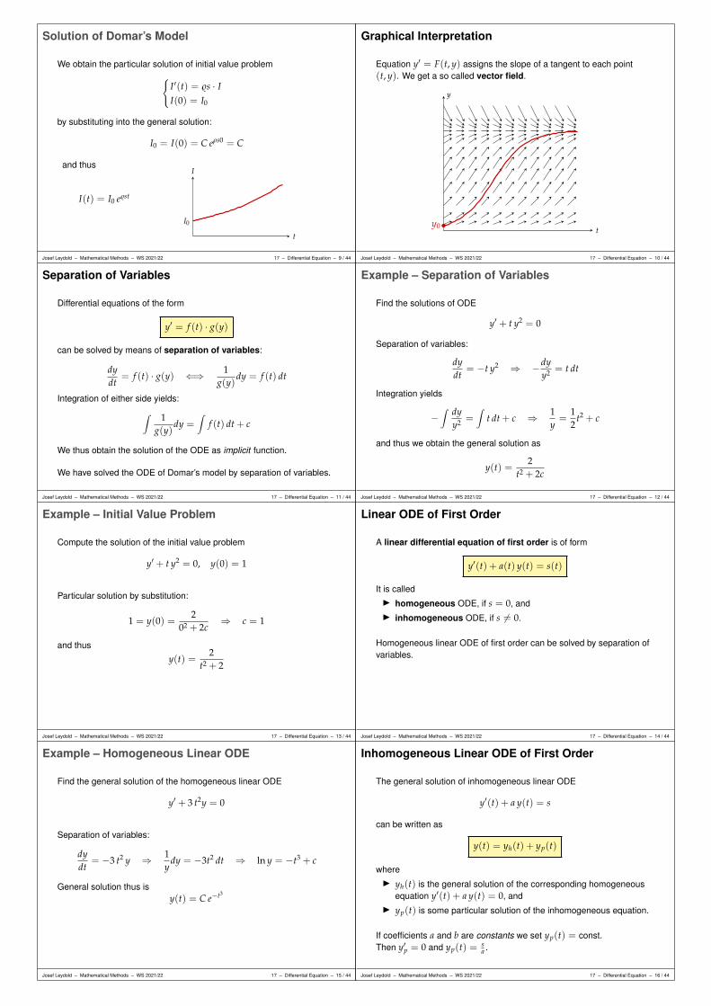
Solution of Domar’s Model
We obtain the particular solution of initial value problem
I′(t) = $s · II(0) = I0
by substituting into the general solution:
I0 = I(0) = C eρs0 = C
and thusI
t
I0
I(t) = I0 e$st
Josef Leydold – Mathematical Methods – WS 2021/22 17 – Differential Equation – 9 / 44
Graphical Interpretation
Equation y′ = F(t, y) assigns the slope of a tangent to each point(t, y). We get a so called vector field.
y
ty0
Josef Leydold – Mathematical Methods – WS 2021/22 17 – Differential Equation – 10 / 44
Separation of Variables
Differential equations of the form
y′ = f (t) · g(y)
can be solved by means of separation of variables:
dydt
= f (t) · g(y) ⇐⇒ 1g(y)
dy = f (t) dt
Integration of either side yields:
∫ 1g(y)
dy =∫
f (t) dt + c
We thus obtain the solution of the ODE as implicit function.
We have solved the ODE of Domar’s model by separation of variables.
Josef Leydold – Mathematical Methods – WS 2021/22 17 – Differential Equation – 11 / 44
Example – Separation of Variables
Find the solutions of ODE
y′ + t y2 = 0
Separation of variables:
dydt
= −t y2 ⇒ −dyy2 = t dt
Integration yields
−∫ dy
y2 =∫
t dt + c ⇒ 1y=
12
t2 + c
and thus we obtain the general solution as
y(t) =2
t2 + 2c
Josef Leydold – Mathematical Methods – WS 2021/22 17 – Differential Equation – 12 / 44
Example – Initial Value Problem
Compute the solution of the initial value problem
y′ + t y2 = 0, y(0) = 1
Particular solution by substitution:
1 = y(0) =2
02 + 2c⇒ c = 1
and thus
y(t) =2
t2 + 2
Josef Leydold – Mathematical Methods – WS 2021/22 17 – Differential Equation – 13 / 44
Linear ODE of First Order
A linear differential equation of first order is of form
y′(t) + a(t) y(t) = s(t)
It is calledI homogeneous ODE, if s = 0, andI inhomogeneous ODE, if s 6= 0.
Homogeneous linear ODE of first order can be solved by separation ofvariables.
Josef Leydold – Mathematical Methods – WS 2021/22 17 – Differential Equation – 14 / 44
Example – Homogeneous Linear ODE
Find the general solution of the homogeneous linear ODE
y′ + 3 t2y = 0
Separation of variables:
dydt
= −3 t2 y ⇒ 1y
dy = −3t2 dt ⇒ ln y = −t3 + c
General solution thus isy(t) = C e−t3
Josef Leydold – Mathematical Methods – WS 2021/22 17 – Differential Equation – 15 / 44
Inhomogeneous Linear ODE of First Order
The general solution of inhomogeneous linear ODE
y′(t) + a y(t) = s
can be written as
y(t) = yh(t) + yp(t)
whereI yh(t) is the general solution of the corresponding homogeneous
equation y′(t) + a y(t) = 0, andI yp(t) is some particular solution of the inhomogeneous equation.
If coefficients a and b are constants we set yp(t) = const.Then y′p = 0 and yp(t) = s
a .
Josef Leydold – Mathematical Methods – WS 2021/22 17 – Differential Equation – 16 / 44

Inhomogeneous Linear ODE of First Order
For the case where all coefficients a and b are constants and non-zerothe general solution of
y′(t) + a y(t) = s
is given as
y(t) = C e−at +sa
Observe that C e−at is just the solution of the correspondinghomogeneous ODE y′(t) + a y(t) = 0.
Josef Leydold – Mathematical Methods – WS 2021/22 17 – Differential Equation – 17 / 44
Inhomogeneous Linear ODE of First Order
For the initial value problem
y′(t) + a y(t) = s, y(0) = y0
we obtain the particular solution
y(t) = (y0 − y) e−at + y with y =sa
We find this solution by substituting the initial value into the particularsolution.
Josef Leydold – Mathematical Methods – WS 2021/22 17 – Differential Equation – 18 / 44
Example – Inhomogeneous Linear ODE
Find the solution of the initial value problem
y′ − 3y = 6, y(0) = 1
We find
y =sa=
6−3
= −2
y(t) = (y0 − y) e−at + y = (1− (−2)) e3t − 2 = 3e3t − 2
The particular solution thus is
y(t) = 3e3t − 2
Josef Leydold – Mathematical Methods – WS 2021/22 17 – Differential Equation – 19 / 44
Model – Dynamic of Market Price
Assume that demand and supply functions are linear:
qd(t) = α− β p(t) (α, β > 0)qs(t) = −γ + δ p(t) (γ, δ > 0)
The rate of price change is directly proportional to the difference(qd − qs):
dpdt
= j (qd(t)− qs(t)) (j > 0)
How does price p(t) evolve in time?
dpdt
= j (qd − qs) = j (α− βp− (−γ + δp))
= j (α + γ)− j (β + δ)p
i.e., we obtain the inhomogeneous linear ODE of first order
p′(t) + j (β + δ) p(t) = j (α + γ)
Josef Leydold – Mathematical Methods – WS 2021/22 17 – Differential Equation – 20 / 44
Model – Dynamic of Market Price
The solution of initial value problem
p′(t) + j (β + δ) p(t) = j (α + γ), p(0) = p0
isp(t) = (p0 − p) e−j(β+δ)t + p
with
p =sa=
j(α + γ)
j(β + δ)=
α + γ
β + δ
Observe that p is just theprice in market equilibrium.
t
p
p0
p0
Josef Leydold – Mathematical Methods – WS 2021/22 17 – Differential Equation – 21 / 44
Logistic Differential Equation
A logistic differential equation is of form
y′(t)− k y(t) (L− y(t)) = 0
where k, L > 0 and 0 ≤ y(t) ≤ L.
I y ≈ 0: y′(t)− k L y(t) ≈ 0 ⇒ y(t) ≈ C ek L t
I y ≈ L: y′(t) + k L y(t) ≈ k L2 ⇒ y(t) ≈ L− C e−k L t
t
L
C ek L t
L− C e−k L t
Josef Leydold – Mathematical Methods – WS 2021/22 17 – Differential Equation – 22 / 44
Logistic Differential Equation
We can find general solution by separation of variables:
y(t) =L
1 + C e−L k t
All solutions have an inflection point in y = L2 .
t
L
L2
Josef Leydold – Mathematical Methods – WS 2021/22 17 – Differential Equation – 23 / 44
Example – Logistic Differential Equation
A flu epidemic happens in a city with 8100 inhabitants. When theepidemic has been detected 100 persons have been infected. Twentydays later 1000 persons have been infected. It is expected that allinhabitants eventually will be infected.Give a model for the number of infected persons.
We use a logistic ODE with L = 8100.Let q(t) denote the number of infected persons,where q(0) = 100 and q(20) = 1000.
The general solution of this ODE is
q(t) =8100
1 + C e−8100kt
We have to estimate parameters k and C.
Josef Leydold – Mathematical Methods – WS 2021/22 17 – Differential Equation – 24 / 44

Example – Logistic Differential Equation
q(0) = 100 ⇒ 81001 + C
= 100 ⇒ C = 80
q(20) = 1000 ⇒ 81001 + 80 e−8100·20 k = 1000 ⇒ k = 0.00001495
The number of infected persons can be described by means of function
q(t) =8100
1 + 80 e−0.121 t .
Josef Leydold – Mathematical Methods – WS 2021/22 17 – Differential Equation – 25 / 44
Differential Equation of Second Order
An ordinary differential equation (ODE) of second order is anequation where the unknown is a univariate function and whichcontains the second (but not any higher) derivative of that function.
y′′ = F(t, y, y′)
We restrict our interest to linear differential equations of secondorder with constant coefficients:
y′′(t) + a1 y′(t) + a2 y(t) = s
Josef Leydold – Mathematical Methods – WS 2021/22 17 – Differential Equation – 26 / 44
Homogeneous Linear ODE of Second Order
We obtain the general solution of the homogeneous linear ODE
y′′(t) + a1 y′(t) + a2 y(t) = 0
by means of the ansatzy(t) = C eλt
where λ satisfies the characteristic equation
λ2 + a1λ + a2 = 0
This condition immediately follows from
y′′(t) + a1 y′(t) + a2 y(t) = λ2 C eλt + a1 λ C eλt + a2 C eλt
= C eλt(λ2 + a1 λ + a2) = 0
Josef Leydold – Mathematical Methods – WS 2021/22 17 – Differential Equation – 27 / 44
Characteristic Equation
The characteristic equation
λ2 + a1λ + a2 = 0
has solutions
λ1,2 = − a1
2±√
a21
4− a2
We have three cases:
1. a21
4 − a2 > 0: two distinct real solutions
2. a21
4 − a2 = 0: exactly one real solution
3. a21
4 − a2 < 0: two complex (non-real) solutions
Josef Leydold – Mathematical Methods – WS 2021/22 17 – Differential Equation – 28 / 44
Case: a21
4 − a2 > 0
The general solution of the homogeneous ODE is given by
y(t) = C1 eλ1t + C2 eλ2t , with λ1,2 = − a1
2±√
a21
4− a2
where C1 and C2 are arbitrary real numbers.
Josef Leydold – Mathematical Methods – WS 2021/22 17 – Differential Equation – 29 / 44
Example: a21
4 − a2 > 0
Compute the general solution of ODE
y′′ − y′ − 2y = 0 .
Characteristic equationλ2 − λ− 2 = 0
has distinct real solutions
λ1 = −1 and λ2 = 2 .
Thus the general solution of the homogeneous ODE is given by
y(t) = C1e−t + C2e2t .
Josef Leydold – Mathematical Methods – WS 2021/22 17 – Differential Equation – 30 / 44
Case: a21
4 − a2 = 0
The general solution of the homogeneous ODE is given by
y(t) = (C1 + C2 t) eλt , with λ = − a1
2
We can verify the validity of solution t eλt by a simple (but tedious)straight-forward computation.
Josef Leydold – Mathematical Methods – WS 2021/22 17 – Differential Equation – 31 / 44
Example: a21
4 − a2 = 0
Compute the general solution of ODE
y′′ + 4y′ + 4y = 0 .
Characteristic equation
λ2 + 4λ + 4 = 0
has the unique solutionλ = −2 .
The general solution of the homogeneous ODE is thus given by
y(t) = (C1 + C2t) e−2t .
Josef Leydold – Mathematical Methods – WS 2021/22 17 – Differential Equation – 32 / 44

Case: a21
4 − a2 < 0
In this case root√
a21
4 − a2 is a non-real (imaginary) number.
From the rules for complex numbers one can derive purely realsolutions:
y(t) = eat [C1 cos(bt) + C2 sin(bt)]
with a = − a12 and b =
√∣∣∣ a21
4 − a2
∣∣∣
Notice that a is the real part of the solution of the characteristicequation and b the imaginary part.Computations with complex numbers however are beyond the scope ofthis course.
Josef Leydold – Mathematical Methods – WS 2021/22 17 – Differential Equation – 33 / 44
Example: a21
4 − a2 < 0
Compute the general solution of ODE
y′′ + y′ + y = 0 .
Characteristic equationλ2 + λ + 1 = 0
does not have real solutions as a21
4 − a2 = 14 − 1 = − 3
4 < 0.
a = − a12 = − 1
2 and b =
√∣∣∣ a21
4 − a2
∣∣∣ =√
34 =
√3
2
The general solution of the homogeneous ODE is thus given by
y(t) = e−12 t[C1 cos
(√3
2 t)+ C2 sin
(√3
2 t)]
.
Josef Leydold – Mathematical Methods – WS 2021/22 17 – Differential Equation – 34 / 44
Inhomogeneous Linear ODE of Second Order
We obtain the general solution of the inhomogeneous ODE
y′′(t) + a1 y′(t) + a2 y(t) = s
by mean so (provide that a2 6= 0)
y(t) = yh(t) +sa2
where yh(t) is the general solution of the corresponding homogeneousODE
y′′h (t) + a1 y′h(t) + a2 yh(t) = 0 .
Josef Leydold – Mathematical Methods – WS 2021/22 17 – Differential Equation – 35 / 44
Example – Inhomogeneous Linear ODE of Second Order
Compute the general solution of ODE
y′′(t) + y′(t)− 2y(t) = −10
Characteristic equation of the homogeneous ODE
λ2 + λ− 2 = 0
has real solutionsλ1 = 1 and λ2 = −2 .
The general solution of the inhomogeneous ODE is thus given by
y(t) = C1 eλ1t + C2 eλ2t +sa2
= C1 et + C2 e−2t +−10−2
.
Josef Leydold – Mathematical Methods – WS 2021/22 17 – Differential Equation – 36 / 44
Initial Value Problem
All general solutions of linear ODEs of second order contain twoindependent integration constants C1 and C2.
Consequently we need two initial values for the particular solution of theinitial value problem
y′′(t) + a1 y′(t) + a2 y(t) = sy(t0) = y0
y′(t0) = y′0
Josef Leydold – Mathematical Methods – WS 2021/22 17 – Differential Equation – 37 / 44
Example – Initial Value Problem
Find the particular solution of initial value problem
y′′(t) + y′(t)− 2y(t) = −10, y(0) = 12, y′(0) = −2 .
Its general solution is given by
y(t) = C1 et + C2 e−2t + 5
y′(t) = C1 et − 2C2 e−2t
Substitution of the initial values yields equations
12 = y(0) = C1 + C2
−2 = y′(0) = C1 − 2C2
with solutions C1 = 4 and C2 = 3.Thus the particular solution of the initial value problem is given by
y(t) = 4et + 3e−2t + 5 .
Josef Leydold – Mathematical Methods – WS 2021/22 17 – Differential Equation – 38 / 44
Fixed Point of an ODE
The inhomogeneous linear ODE
y′′(t) + a1 y′(t) + a2 y(t) = s
has the special constant solution
y(t) = y =sa2
(= constant)
Point y is called fixed point, stationary point, or equilibrium point ofthe ODE.
Josef Leydold – Mathematical Methods – WS 2021/22 17 – Differential Equation – 39 / 44
Stable and Unstable Fixed Points
The value of a determines the qualitative behavior of solution curve
y(t) = eat [C1 cos(bt) + C2 sin(bt)]+ y .
t t t
a < 0 a = 0 a > 0
stable fixed point unstable fixed point
Josef Leydold – Mathematical Methods – WS 2021/22 17 – Differential Equation – 40 / 44
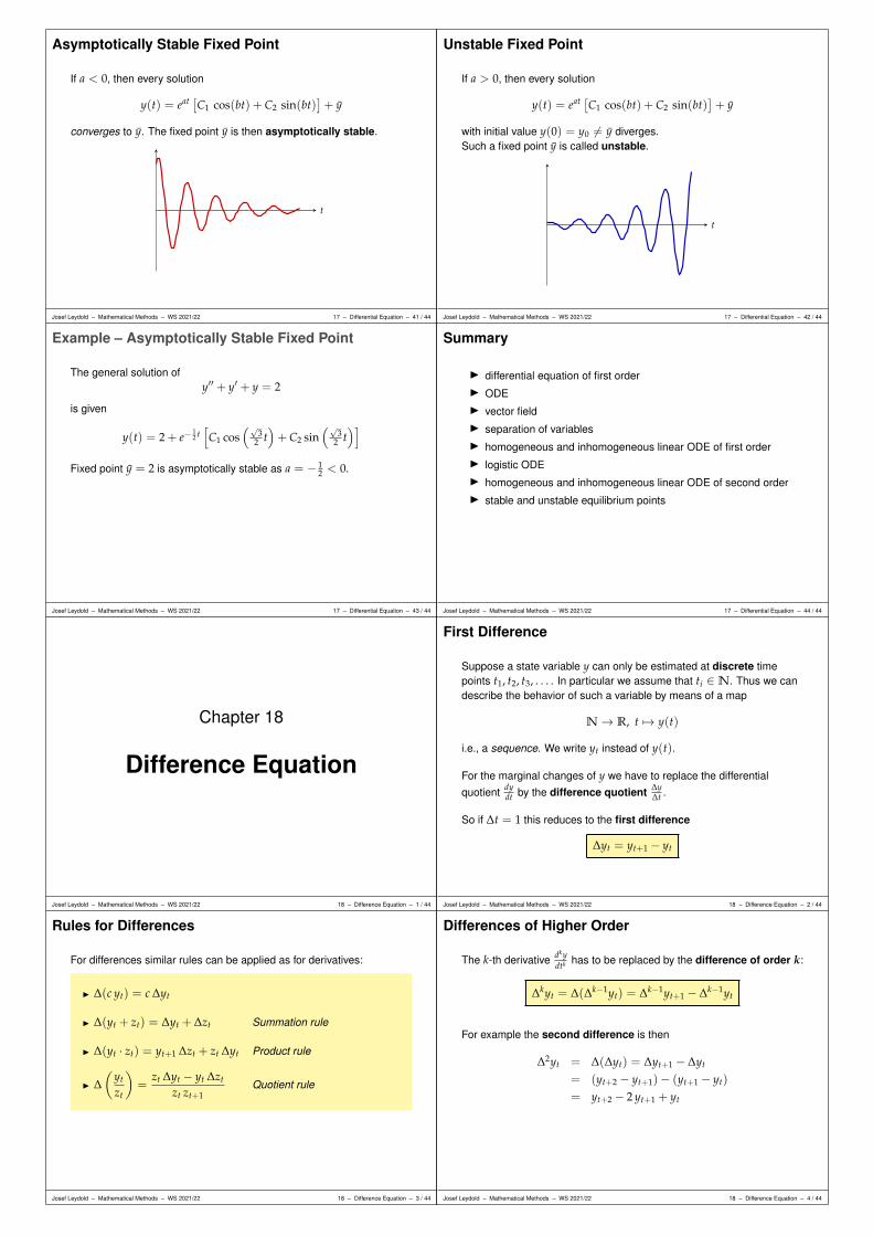
Asymptotically Stable Fixed Point
If a < 0, then every solution
y(t) = eat [C1 cos(bt) + C2 sin(bt)]+ y
converges to y. The fixed point y is then asymptotically stable.
t
Josef Leydold – Mathematical Methods – WS 2021/22 17 – Differential Equation – 41 / 44
Unstable Fixed Point
If a > 0, then every solution
y(t) = eat [C1 cos(bt) + C2 sin(bt)]+ y
with initial value y(0) = y0 6= y diverges.Such a fixed point y is called unstable.
t
Josef Leydold – Mathematical Methods – WS 2021/22 17 – Differential Equation – 42 / 44
Example – Asymptotically Stable Fixed Point
The general solution ofy′′ + y′ + y = 2
is given
y(t) = 2 + e−12 t[C1 cos
(√3
2 t)+ C2 sin
(√3
2 t)]
Fixed point y = 2 is asymptotically stable as a = − 12 < 0.
Josef Leydold – Mathematical Methods – WS 2021/22 17 – Differential Equation – 43 / 44
Summary
I differential equation of first orderI ODEI vector fieldI separation of variablesI homogeneous and inhomogeneous linear ODE of first orderI logistic ODEI homogeneous and inhomogeneous linear ODE of second orderI stable and unstable equilibrium points
Josef Leydold – Mathematical Methods – WS 2021/22 17 – Differential Equation – 44 / 44
Chapter 18
Difference Equation
Josef Leydold – Mathematical Methods – WS 2021/22 18 – Difference Equation – 1 / 44
First Difference
Suppose a state variable y can only be estimated at discrete timepoints t1, t2, t3, . . . . In particular we assume that ti ∈N. Thus we candescribe the behavior of such a variable by means of a map
N→ R, t 7→ y(t)
i.e., a sequence. We write yt instead of y(t).
For the marginal changes of y we have to replace the differentialquotient dy
dt by the difference quotient ∆y∆t .
So if ∆t = 1 this reduces to the first difference
∆yt = yt+1 − yt
Josef Leydold – Mathematical Methods – WS 2021/22 18 – Difference Equation – 2 / 44
Rules for Differences
For differences similar rules can be applied as for derivatives:
I ∆(c yt) = c ∆yt
I ∆(yt + zt) = ∆yt + ∆zt Summation rule
I ∆(yt · zt) = yt+1 ∆zt + zt ∆yt Product rule
I ∆(
yt
zt
)=
zt ∆yt − yt ∆zt
zt zt+1Quotient rule
Josef Leydold – Mathematical Methods – WS 2021/22 18 – Difference Equation – 3 / 44
Differences of Higher Order
The k-th derivative dkydtk has to be replaced by the difference of order k:
∆kyt = ∆(∆k−1yt) = ∆k−1yt+1 − ∆k−1yt
For example the second difference is then
∆2yt = ∆(∆yt) = ∆yt+1 − ∆yt
= (yt+2 − yt+1)− (yt+1 − yt)
= yt+2 − 2 yt+1 + yt
Josef Leydold – Mathematical Methods – WS 2021/22 18 – Difference Equation – 4 / 44

Difference Equation
A difference equation is an equation that contains the differences of asequence. It is of order n if it contains a difference of order n (but nothigher).
∆yt = 3 difference equation of first order
∆yt =12 yt difference equation of first order
∆2yt + 2 ∆yt = −3 difference equation of second order
If in addition an initial value y0 is givenwe have a so called initial value problem.
Josef Leydold – Mathematical Methods – WS 2021/22 18 – Difference Equation – 5 / 44
Equivalent Representation
Difference equations can equivalently written without ∆-notation.
∆yt = 3 ⇔ yt+1 − yt = 3 ⇔ yt+1 = yt + 3
∆yt =12 yt ⇔ yt+1 − yt =
12 yt ⇔ yt+1 = 3
2 yt
∆2yt + 2 ∆yt = −3 ⇔⇔ (yt+2 − 2 yt+1 + yt) + 2 (yt+1 − yt) = −3
⇔ yt+2 = yt − 3
These can be seen as recursion formulæ for sequences.
Problem:Find a sequence yt which satisfies the given recursion formula for allt ∈N.
Josef Leydold – Mathematical Methods – WS 2021/22 18 – Difference Equation – 6 / 44
Initial Value Problem and Iterations
Difference equations of first order can be solved by iterativelycomputing the elements of the sequence if the initial value y0 is given.
Compute the solution of yt+1 = yt + 3 with initial value y0.
y1 = y0 + 3y2 = y1 + 3 = (y0 + 3) + 3 = y0 + 2 · 3y3 = y2 + 3 = (y0 + 2 · 3) + 3 = y0 + 3 · 3. . .yt = y0 + 3 t
For initial value y0 = 5 we obtain yt = 5 + 3 t.
Josef Leydold – Mathematical Methods – WS 2021/22 18 – Difference Equation – 7 / 44
Example – Iterations
Compute the solution of yt+1 = 32 yt with initial value y0.
y1 = 32 y0
y2 = 32 y1 = 3
2 (32 y0) =
( 32
)2 y0
y3 = 32 y2 = 3
2 (32
2y0) =( 3
2
)3 y0
. . .yt =
( 32
)t y0
For initial value y0 = 5 we obtain yt = 5 ·( 3
2
)t.
Josef Leydold – Mathematical Methods – WS 2021/22 18 – Difference Equation – 8 / 44
Homogeneous Linear Difference Equation of First Order
A homogeneous linear difference equation of first order is of form
yt+1 + a yt = 0
Ansatz for general solution:
yt = C βt, C β 6= 0, for some fixed C ∈ R.
It has to satisfy the difference equation for all t:
yt+1 + a yt = C βt+1 + a C βt = 0.
Division by C βt yields β + a = 0 and thus β = −a and
yt = C (−a)t
Josef Leydold – Mathematical Methods – WS 2021/22 18 – Difference Equation – 9 / 44
Example – Homogeneous Equation
Homogeneous linear difference equation
yt+1 −32
yt = 0
has general solution
yt = C(
32
)t
.
Josef Leydold – Mathematical Methods – WS 2021/22 18 – Difference Equation – 10 / 44
Properties of Solutions
The behavior of solution
yt = C βt = C (−a)t
obviously depends on parameter β = −a which can be summarized asfollowing:
oscillating ⇔ β < 0convergent ⇔ |β| < 1
We want to note that β is the root of the characteristic equationβ + a = 0.
Josef Leydold – Mathematical Methods – WS 2021/22 18 – Difference Equation – 11 / 44
Properties of Solutions
yt
t
yt
t
yt
t
β > 1 β = 1 0 < β < 1
yt
t
yt
t
yt
t
−1 < β < 0 β = −1 β < −1
Josef Leydold – Mathematical Methods – WS 2021/22 18 – Difference Equation – 12 / 44
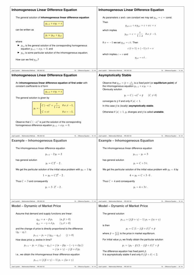
Inhomogeneous Linear Difference Equation
The general solution of inhomogeneous linear difference equation
yt+1 + a yt = s
can be written as
yt = yh,t + yp,t
whereI ph,t is the general solution of the corresponding homogeneous
equation yt+1 + a yt = 0, andI yh,t is some particular solution of the inhomogeneous equation.
How can we find yp,t?
Josef Leydold – Mathematical Methods – WS 2021/22 18 – Difference Equation – 13 / 44
Inhomogeneous Linear Difference Equation
As parameters a and s are constant we may set yh,t = c = const.
Thenyp,t+1 + a yp,t = c + a c = s
which implies
yp,t = c =s
1 + aif a 6= −1.
If a = −1 we set yp,t = c t. Then
c (t + 1) + (−1) c t = s
which implies c = s andyp,t = s t .
Josef Leydold – Mathematical Methods – WS 2021/22 18 – Difference Equation – 14 / 44
Inhomogeneous Linear Difference Equation
An inhomogeneous linear difference equation of first order withconstant coefficients is of form
yt+1 + a yt = s
The general solution is given by
yt =
C (−a)t +s
1 + aif a 6= −1,
C + s t if a = −1.
Observe that C (−a)t is just the solution of the correspondinghomogeneous difference equation yt+1 + a yt = 0.
Josef Leydold – Mathematical Methods – WS 2021/22 18 – Difference Equation – 15 / 44
Asymptotically Stable
Observe that yp,t = y = s1+a is a fixed point (or equilibrium point) of
the inhomogeneous equation yt+1 + a yt = s.Obviously solution
yt = C (−a)t + y (C 6= 0)
converges to y if and only if |a| < 1.
In this case y is (locally ) asymptotically stable.
Otherwise if |a| > 1, yt diverges and y is called unstable.
Josef Leydold – Mathematical Methods – WS 2021/22 18 – Difference Equation – 16 / 44
Example – Inhomogeneous Equation
The inhomogeneous linear difference equation
yt+1 − 2 yt = 2
has general solutionyt = C 2t − 2 .
We get the particular solution of the initial value problem with y0 = 1 by
1 = y0 = C 20 − 2 .
Thus C = 3 and consequently
yt = 3 · 2t − 2 .
Josef Leydold – Mathematical Methods – WS 2021/22 18 – Difference Equation – 17 / 44
Example – Inhomogeneous Equation
The inhomogeneous linear difference equation
yt+1 − yt = 3
has general solutionyt = C + 3 t.
We get the particular solution of the initial value problem with y0 = 4 by
4 = y0 = C + 3 · 0 .
Thus C = 4 and consequently
yt = 4 + 3 t .
Josef Leydold – Mathematical Methods – WS 2021/22 18 – Difference Equation – 18 / 44
Model – Dynamic of Market Price
Assume that demand and supply functions are linear:
qd,t = α− β pt (α, β > 0)qs,t = −γ + δ pt (γ, δ > 0)
and the change of price is directly proportional to the difference(qd − qs):
pt+1 − pt = j (qd,t − qs,t) (j > 0)
How does price pt evolve in time?
pt+1 − pt = j (qd,t − qs,t) = j (α− βpt − (−γ + δpt))
= j (α + γ)− j (β + δ)pt
i.e., we obtain the inhomogeneous linear difference equation
pt+1 + (j(β + γ)− 1) pt = j(α + γ)
Josef Leydold – Mathematical Methods – WS 2021/22 18 – Difference Equation – 19 / 44
Model – Dynamic of Market Price
The general solution
pt+1 + (j(β + γ)− 1) pt = j(α + γ)
is thenpt = C (1− j(β + δ))t + p
where p = α+γβ+δ is the price in market equilibrium.
For initial value p0 we finally obtain the particular solution
pt = (p0 − p)(1− j(β + δ))t + p
The difference equation has fixed point p.It is asymptotically stable if and only if j(β + δ) < 2.
Josef Leydold – Mathematical Methods – WS 2021/22 18 – Difference Equation – 20 / 44

Model – Dynamic of Market Price
Consider the following market model:
qd,t = qs,t
qd,t = α− βpt (α, β > 0)qs,t = −γ + δpt−1 (γ, δ > 0)
Observe that we have market equilibrium in each period.The supply depends on the price of the preceding period.Substituting of the second and third equation onto the first yields theinhomogeneous linear difference equation
β pt + δ pt−1 = α + γ ⇔ pt+1 +δ
βpt =
α + γ
β
Josef Leydold – Mathematical Methods – WS 2021/22 18 – Difference Equation – 21 / 44
Model – Dynamic of Market Price
Inhomogeneous linear first order difference equation
pt+1 +δ
βpt =
α + γ
β
with initial value p0 has solution
pt = (p0 − p)(− δ
β
)t
+ p where p =α + γ
β + δ.
As all constants are positive, root − δβ < 0 and thus all solutions of such
a market model oscillate.
The solution converges to the p if∣∣∣ δ
β
∣∣∣ < 1.
Josef Leydold – Mathematical Methods – WS 2021/22 18 – Difference Equation – 22 / 44
Cobweb Model
We also can analyze this model graphically.Demand and supply are functions of price p:
D(p) = α− βp, and S(p) = −γ + δp
qt
pt
S
Dp0p1 p2p3 p4
q1
q2
q3
q4
q5
p
qt
pt
S
Dp0p1 p2p3 p4
q1
q2
q3
q4
q5
p
δ > β δ < β
Josef Leydold – Mathematical Methods – WS 2021/22 18 – Difference Equation – 23 / 44
Cobweb Model
↑ We start in period 0 with pricep0 and get supply q1 = S(p0)in period 1.
← Market equilibrium implies newprice p1 given implicitly byD(p1) = q1.
↓ In period 2 price p1 yieldssupply q2 = S(p1).
→ Market equilibrium implies newprice p2 given implicitly byD(p2) = q2.
qt
pt
S
Dp0p1 p2p3 p4
q1
q2
q3
q4
q5
p
q
Iterating this procedure spins acobweb around equilibrium point( p, q) with q = S( p) = D( p).
Josef Leydold – Mathematical Methods – WS 2021/22 18 – Difference Equation – 24 / 44
Cobweb Model – Nonlinear Functions
Cobweb models also work when functions D(p) and S(p) arenonlinear.
Then there may not exist a solution in closed form.However, we still have an equilibrium point p with D( p) = S( p).Linearized versions of D and S:
D(p) = D( p) + D′( p)(p− p)
S(p) = S( p) + S′( p)(p− p)
Equilibrium point p is locallyasymptotically stable ifI D′( p) < 0 < S′( p), andI |S′( p)| < |D′( p)|.
qt
ptD
S
p
q
Josef Leydold – Mathematical Methods – WS 2021/22 18 – Difference Equation – 25 / 44
Linear Difference Equation of Second Order
A difference equation is an equation that contains the differences ofsecond order of a sequence.
We restrict our interest to linear difference equations of secondorder with constant coefficients:
yt+2 + a1 yt+1 + a2 yt = s
Josef Leydold – Mathematical Methods – WS 2021/22 18 – Difference Equation – 26 / 44
Homogeneous Linear Difference Equation
We obtain the general solution of the homogeneous linear ODE
yt+2 + a1 yt+1 + a2 yt = 0
by means of the ansatz
yt = C βt, C β 6= 0
which has to satisfies the difference equation :
C βt+2 + a1 C βt+1 + a2 C βt = 0 .
Hence β has to satisfy the characteristic equation
β2 + a1 β + a2 = 0
Josef Leydold – Mathematical Methods – WS 2021/22 18 – Difference Equation – 27 / 44
Characteristic Equation
The characteristic equation
β2 + a1 β + a2 = 0
has solutions
β1,2 = − a1
2±√
a21
4− a2
We have three cases:
1. a21
4 − a2 > 0: two distinct real solutions
2. a21
4 − a2 = 0: exactly one real solution
3. a21
4 − a2 < 0: two complex (non-real) solutions
Josef Leydold – Mathematical Methods – WS 2021/22 18 – Difference Equation – 28 / 44

Case: a21
4 − a2 > 0
The general solution of the homogeneous difference equation
yt+2 + a1 yt+1 + a2 yt = 0
is given by
y(t) = C1 βt1 + C2 βt
2 , with β1,2 = − a1
2±√
a21
4− a2
where C1 and C2 are arbitrary real numbers.
Josef Leydold – Mathematical Methods – WS 2021/22 18 – Difference Equation – 29 / 44
Example: a21
4 − a2 > 0
Compute the general solution of difference equation
yt+2 − 3 yt+1 + 2 yt = 0 .
Characteristic equation
β2 − 3 β + 2 = 0
has distinct real solutions
β1 = 1 and β2 = 2 .
Thus the general solution of the homogeneous equation is given by
yt = C1 1t + C2 2t = C1 + C2 2t .
Josef Leydold – Mathematical Methods – WS 2021/22 18 – Difference Equation – 30 / 44
Case: a21
4 − a2 = 0
The general solution of the homogeneous difference equation
yt+2 + a1 yt+1 + a2 yt = 0
is given by
yt = C1 βt + C2 t βt , with β = − a1
2
We can verify the validity of solution t βt by a simple (but tedious)straight-forward computation.
Josef Leydold – Mathematical Methods – WS 2021/22 18 – Difference Equation – 31 / 44
Example: a21
4 − a2 = 0
Compute the general solution of difference equation
yt+2 − 4 yt+1 + 4 yt = 0 .
Characteristic equation
β2 − 4 β + 4 = 0
has the unique solutionβ = 2 .
Thus the general solution of the homogeneous equation is given by
yt = C1 2t + C2 t 2t .
Josef Leydold – Mathematical Methods – WS 2021/22 18 – Difference Equation – 32 / 44
Case: a21
4 − a2 < 0
In this case root√
a21
4 − a2 is a non-real (imaginary) number:
β1,2 = a± b i
whereI a = − a1
2 is called the real part, and
I b =
√∣∣∣a2 − a21
4
∣∣∣ the imaginary part of root β.
Alternatively β can be represent by so called polar coordinates
β1,2 = r(cos θ ± i sin θ)
where
I r = |β| =√
a2 + b2 =
√a2
14 + a2 − a2
14 =√
a2is called the modulus (or absolute value) of β, and
I θ = arg(β) the argument of β.
Josef Leydold – Mathematical Methods – WS 2021/22 18 – Difference Equation – 33 / 44
Modulus and Argument
A complex number z = a + b i can beinterpreted as point (a, b) in the (real) plane.
This point can also can be given by polarcoordinates withradius r = |z| (absolute value or modulus),and angle θ (called the argument of z).
θ
rr sin θ
r cos θ
(a, b)
We then have
r = |z| =√
a2 + b2
and
tan θ =ba
because cos θ = ar and sin θ = b
r .
Josef Leydold – Mathematical Methods – WS 2021/22 18 – Difference Equation – 34 / 44
Case: a21
4 − a2 < 0
From the rules for complex numbers one can derive purely realsolutions of the homogeneous difference equation
yt+2 + a1 yt+1 + a2 yt = 0
given by
yt = rt [C1 cos(θt) + C2 sin(θt)]
with r = |β| = √a2 and θ = arg(β)
Argument arg(β) is given by
cos θ = ar = − a1
2√
a2
sin θ = br =
√1− a2
14 a2
Josef Leydold – Mathematical Methods – WS 2021/22 18 – Difference Equation – 35 / 44
Example: a21
4 − a2 < 0
Compute the general solution of difference equation
yt+2 + 2 yt+1 + 4 yt = 0 .
Characteristic equation
β2 + 2 β + 4 = 0
has the complex solutions
β1,2 = −1±√
3 i
i.e., a = −1 and b =√
3.
Josef Leydold – Mathematical Methods – WS 2021/22 18 – Difference Equation – 36 / 44

Example: a21
4 − a2 < 0
Complex root β = a + b i with a = −1 and b =√
3has polar coordinates:I r =
√12 + 3 =
√4 = 2, and
I θ = 2π3 , as sin θ = a
r = − 12 and cos θ = b
r =√
32 .
Thus the general solution of the homogeneous equation is given by
yt = 2t[
C1 cos(
2π
3t)+ C2 sin
(2π
3t)]
.
Argument θ can be computed by means of the arcus tangens functionarctan(b/a).A more convenient way is to use function atan2 which is available inprograms like R.
Josef Leydold – Mathematical Methods – WS 2021/22 18 – Difference Equation – 37 / 44
Inhomogeneous Linear Difference Equation
The general solution of inhomogeneous linear difference equation
yt+2 + a1 yt+1 + a2 yt = s
can be written as
yt = yh,t + yp,t
whereI yh,t is the general solution of the corresponding homogeneous
equation yt+2 + a1 yt+1 + a2 yt = s, andI yh,t is some particular solution of the inhomogeneous equation.
How can we find yp,t?
Josef Leydold – Mathematical Methods – WS 2021/22 18 – Difference Equation – 38 / 44
Inhomogeneous Linear Difference Equation
By assumption all coefficients a1, a2, and s. So we may assume thatyp,t = c = const:
c + a1 c + a2 c = s
which implies
yp,t = c =s
1 + a1 + a2if a1 + a2 6= −1.
If a1 + a2 6= −1 we may use yp,t = ct and get
yp,t =s
a1 + 2t if a1 + a2 = −1 and a1 6= −2.
Josef Leydold – Mathematical Methods – WS 2021/22 18 – Difference Equation – 39 / 44
Example – Inhomogeneous Equation
Compute the general solution of difference equation
yt+2 + 2 yt+1 + 4 yt = 14 .
General solution of homogeneous equation yt+2 + 2 yt+1 + 4 yt = 0:
yh,t = 2t[
C1 cos(
2π
3t)+ C2 sin
(2π
3t)]
.
As a1 + a2 = 2 + 4 6= −1 we use yp,t =14
1+2+4 = 2 and obtain thegeneral solution of the inhomogeneous equation as
yt = yh,t + yp,t = 2t[
C1 cos(
2π
3t)+ C2 sin
(2π
3t)]
+ 2 .
Josef Leydold – Mathematical Methods – WS 2021/22 18 – Difference Equation – 40 / 44
Example – Inhomogeneous Equation
Compute the general solution of difference equation
yt+2 − 3 yt+1 + 2 yt = 2 .
General solution of homogeneous equation yt+2 − 3 yt+1 + 2 yt = 0:
yh,t = C1 + C22t .
As a1 + a2 = −3 + 2 = −1 and a1 6= −2 we use yp,t =2
−3+2 t = −2tand obtain the general solution of the inhomogeneous equation as
yt = yh,t + yp,t = C1 + C22t − 2t .
Josef Leydold – Mathematical Methods – WS 2021/22 18 – Difference Equation – 41 / 44
Fixed Point of a Difference Equation
The inhomogeneous linear difference equation
yt+2 + a1 yt+1 + a2 yt = s
has the special constant solution (for a1 + a2 6= −1)
yp,t = y =s
1 + a1 + a2(= constant)
Point y is called fixed point, or equilibrium point of the differenceequation.
Josef Leydold – Mathematical Methods – WS 2021/22 18 – Difference Equation – 42 / 44
Stable and Unstable Fixed Points
When we review general solutions of linear difference equations (withconstant coefficients) we observe that these solutions converge to afixed point y for all choices of constants C if the absolute values of theroots β of the characteristic equation are less than one:
yt → y for t→ ∞ if |β| < 1.
In this case y is called an asymptotically stable fixed point.
Josef Leydold – Mathematical Methods – WS 2021/22 18 – Difference Equation – 43 / 44
Summary
I differences of sequencesI difference equationI homogeneous and inhomogeneous linear difference equation of
first order with constant coefficientsI cobweb modelI homogeneous and inhomogeneous linear difference equation of
second order with constant coefficientsI stable and unstable fixed points
Josef Leydold – Mathematical Methods – WS 2021/22 18 – Difference Equation – 44 / 44
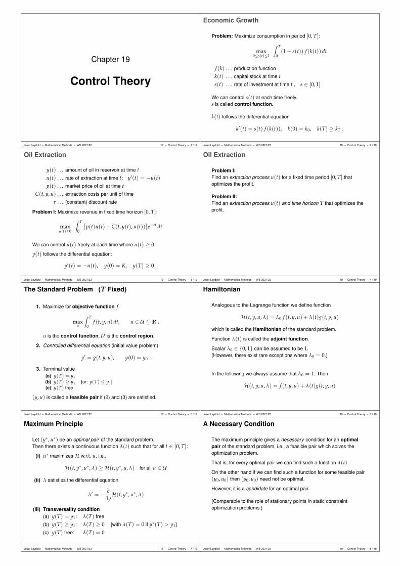
Chapter 19
Control Theory
Josef Leydold – Mathematical Methods – WS 2021/22 19 – Control Theory – 1 / 19
Economic Growth
Problem: Maximize consumption in period [0, T]:
max0≤s(t)≤1
∫ T
0(1− s(t)) f (k(t)) dt
f (k) . . . production function
k(t) . . . capital stock at time ts(t) . . . rate of investment at time t , s ∈ [0, 1]
We can control s(t) at each time freely.s is called control function.
k(t) follows the differential equation
k′(t) = s(t) f (k(t)), k(0) = k0, k(T) ≥ kT .
Josef Leydold – Mathematical Methods – WS 2021/22 19 – Control Theory – 2 / 19
Oil Extraction
y(t) . . . amount of oil in reservoir at time tu(t) . . . rate of extraction at time t: y′(t) = −u(t)p(t) . . . market price of oil at time t
C(t, y, u) . . . extraction costs per unit of time
r . . . (constant) discount rate
Problem I: Maximize revenue in fixed time horizon [0, T]:
maxu(t)≥0
∫ T
0
[p(t)u(t)− C(t, y(t), u(t))
]e−rt dt
We can control u(t) freely at each time where u(t) ≥ 0.
y(t) follows the differential equation:
y′(t) = −u(t), y(0) = K, y(T) ≥ 0 .
Josef Leydold – Mathematical Methods – WS 2021/22 19 – Control Theory – 3 / 19
Oil Extraction
Problem I:Find an extraction process u(t) for a fixed time period [0, T] thatoptimizes the profit.
Problem II:Find an extraction process u(t) and time horizon T that optimizes theprofit.
Josef Leydold – Mathematical Methods – WS 2021/22 19 – Control Theory – 4 / 19
The Standard Problem (T Fixed)
1. Maximize for objective function f
maxu
∫ T
0f (t, y, u) dt, u ∈ U ⊆ R .
u is the control function, U is the control region.
2. Controlled differential equation (initial value problem)
y′ = g(t, y, u), y(0) = y0 .
3. Terminal value(a) y(T) = y1(b) y(T) ≥ y1 [or: y(T) ≤ y1](c) y(T) free
(y, u) is called a feasible pair if (2) and (3) are satisfied.
Josef Leydold – Mathematical Methods – WS 2021/22 19 – Control Theory – 5 / 19
Hamiltonian
Analogous to the Lagrange function we define function
H(t, y, u, λ) = λ0 f (t, y, u) + λ(t)g(t, y, u)
which is called the Hamiltonian of the standard problem.
Function λ(t) is called the adjoint function.
Scalar λ0 ∈ 0, 1 can be assumed to be 1.(However, there exist rare exceptions where λ0 = 0.)
In the following we always assume that λ0 = 1. Then
H(t, y, u, λ) = f (t, y, u) + λ(t)g(t, y, u)
Josef Leydold – Mathematical Methods – WS 2021/22 19 – Control Theory – 6 / 19
Maximum Principle
Let (y∗, u∗) be an optimal pair of the standard problem.Then there exists a continuous function λ(t) such that for all t ∈ [0, T]:
(i) u∗ maximizes H w.r.t. u, i.e.,
H(t, y∗, u∗, λ) ≥ H(t, y∗, u, λ) for all u ∈ U
(ii) λ satisfies the differential equation
λ′ = − ∂
∂yH(t, y∗, u∗, λ)
(iii) Transversality condition(a) y(T) = y1: λ(T) free
(b) y(T) ≥ y1: λ(T) ≥ 0 [with λ(T) = 0 if y∗(T) > y1]
(c) y(T) free: λ(T) = 0
Josef Leydold – Mathematical Methods – WS 2021/22 19 – Control Theory – 7 / 19
A Necessary Condition
The maximum principle gives a necessary condition for an optimalpair of the standard problem, i.e., a feasible pair which solves theoptimization problem.
That is, for every optimal pair we can find such a function λ(t).
On the other hand if we can find such a function for some feasible pair(y0, u0) then (y0, u0) need not be optimal.
However, it is a candidate for an optimal pair.
(Comparable to the role of stationary points in static constraintoptimization problems.)
Josef Leydold – Mathematical Methods – WS 2021/22 19 – Control Theory – 8 / 19
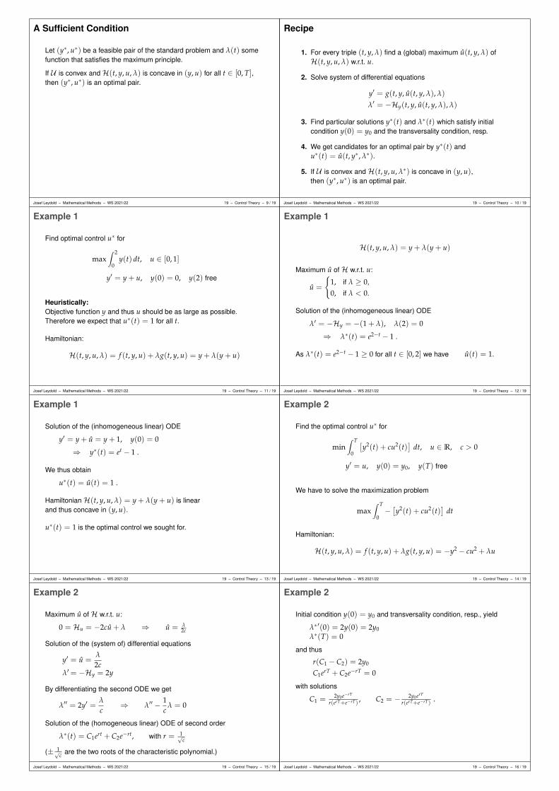
A Sufficient Condition
Let (y∗, u∗) be a feasible pair of the standard problem and λ(t) somefunction that satisfies the maximum principle.
If U is convex and H(t, y, u, λ) is concave in (y, u) for all t ∈ [0, T],then (y∗, u∗) is an optimal pair.
Josef Leydold – Mathematical Methods – WS 2021/22 19 – Control Theory – 9 / 19
Recipe
1. For every triple (t, y, λ) find a (global) maximum u(t, y, λ) ofH(t, y, u, λ) w.r.t. u.
2. Solve system of differential equations
y′ = g(t, y, u(t, y, λ), λ)
λ′ = −Hy(t, y, u(t, y, λ), λ)
3. Find particular solutions y∗(t) and λ∗(t) which satisfy initialcondition y(0) = y0 and the transversality condition, resp.
4. We get candidates for an optimal pair by y∗(t) andu∗(t) = u(t, y∗, λ∗).
5. If U is convex and H(t, y, u, λ∗) is concave in (y, u),then (y∗, u∗) is an optimal pair.
Josef Leydold – Mathematical Methods – WS 2021/22 19 – Control Theory – 10 / 19
Example 1
Find optimal control u∗ for
max∫ 2
0y(t) dt, u ∈ [0, 1]
y′ = y + u, y(0) = 0, y(2) free
Heuristically:Objective function y and thus u should be as large as possible.Therefore we expect that u∗(t) = 1 for all t.
Hamiltonian:
H(t, y, u, λ) = f (t, y, u) + λg(t, y, u) = y + λ(y + u)
Josef Leydold – Mathematical Methods – WS 2021/22 19 – Control Theory – 11 / 19
Example 1
H(t, y, u, λ) = y + λ(y + u)
Maximum u of H w.r.t. u:
u =
1, if λ ≥ 0,
0, if λ < 0.
Solution of the (inhomogeneous linear) ODE
λ′ = −Hy = −(1 + λ), λ(2) = 0
⇒ λ∗(t) = e2−t − 1 .
As λ∗(t) = e2−t − 1 ≥ 0 for all t ∈ [0, 2] we have u(t) = 1.
Josef Leydold – Mathematical Methods – WS 2021/22 19 – Control Theory – 12 / 19
Example 1
Solution of the (inhomogeneous linear) ODE
y′ = y + u = y + 1, y(0) = 0
⇒ y∗(t) = et − 1 .
We thus obtain
u∗(t) = u(t) = 1 .
Hamiltonian H(t, y, u, λ) = y + λ(y + u) is linearand thus concave in (y, u).
u∗(t) = 1 is the optimal control we sought for.
Josef Leydold – Mathematical Methods – WS 2021/22 19 – Control Theory – 13 / 19
Example 2
Find the optimal control u∗ for
min∫ T
0
[y2(t) + cu2(t)
]dt, u ∈ R, c > 0
y′ = u, y(0) = y0, y(T) free
We have to solve the maximization problem
max∫ T
0−[y2(t) + cu2(t)
]dt
Hamiltonian:
H(t, y, u, λ) = f (t, y, u) + λg(t, y, u) = −y2 − cu2 + λu
Josef Leydold – Mathematical Methods – WS 2021/22 19 – Control Theory – 14 / 19
Example 2
Maximum u of H w.r.t. u:
0 = Hu = −2cu + λ ⇒ u = λ2c
Solution of the (system of) differential equations
y′ = u =λ
2cλ′= −Hy = 2y
By differentiating the second ODE we get
λ′′ = 2y′ =λ
c⇒ λ′′ − 1
cλ = 0
Solution of the (homogeneous linear) ODE of second order
λ∗(t) = C1ert + C2e−rt, with r = 1√c
(± 1√c are the two roots of the characteristic polynomial.)
Josef Leydold – Mathematical Methods – WS 2021/22 19 – Control Theory – 15 / 19
Example 2
Initial condition y(0) = y0 and transversality condition, resp., yield
λ∗′(0) = 2y(0) = 2y0λ∗(T) = 0
and thus
r(C1 − C2) = 2y0
C1erT + C2e−rT = 0
with solutions
C1 = 2y0e−rT
r(erT+e−rT), C2 = − 2y0erT
r(erT+e−rT).
Josef Leydold – Mathematical Methods – WS 2021/22 19 – Control Theory – 16 / 19

Example 2
Consequently we obtain
λ∗(t) = 2y0r(erT+e−rT)
(e−r(T−t) − er(T−t)
)
y∗(t) = 12 λ∗(t) = y0
e−r(T−t)−er(T−t)
r(erT+e−rT)
u∗(t) = u(t, y∗, λ∗) = 12c λ∗(t) = y0
ce−r(T−t)−er(T−t)
r(erT+e−rT)
It is easy to verify that Hamiltonian H(t, y, u, λ) = −y2 − cu2 + λu isconcave in y and u.
u∗(t) = y0c
e−r(T−t)−er(T−t)
r(erT+e−rT)is the optimal control.
Josef Leydold – Mathematical Methods – WS 2021/22 19 – Control Theory – 17 / 19
Standard Problem (T Variable)
If time horizon [0, T] is not fixed in advanced we have to find an optimaltime period [0, T∗] in addition to the optimal control u∗.
For this purpose we have to add the following condition to the maximumprinciple (in addition to (i)–(iii)).
(iv) H(T∗, y∗(T∗), u∗(T∗), λ(T∗)) = 0
The recipe for solving the optimization problem remains essentially thesame.
Josef Leydold – Mathematical Methods – WS 2021/22 19 – Control Theory – 18 / 19
Summary
I standard problemI Hamiltonian functionI maximum principleI a sufficient condition
Josef Leydold – Mathematical Methods – WS 2021/22 19 – Control Theory – 19 / 19