long-range oasdi projection methodology · long-range oasdi projection methodology intermediate...

Long-Range OASDI Projection Methodology

Intermediate Assumptions of the 2008 Trustees

Report

June 2008 Office of the Chief Actuary Social Security Administration

I. Flow Charts

Overview of Long-Range OASDI Projection Methodology

Process 2:

EconomicsProcess 1:

Demography

Process 4:

Trust Fund Operations and Actuarial Status

Process 3:

Beneficiaries

Social Security AdministrationOffice of the Chief Actuary

June 2008

Chart 1:

Trustees ultimate assumptionsFertility

MortalityImmigration

1.2 Mortality ratesInputs: Historical number of U.S. deaths by cause and U.S. resident population; medicare deaths and enrollmentsOutputs: Historical and projected death probabilities

1.4 Historical PopulationInputs: Historical U.S. population, undercounts, marital status data and immigration prevalence estimates and estimates of population in other components of Social Security area. Outputs: Historical Social Security area population by age,gender, and marital status (including starting population) Historical other than legal population by age, sex and marital status

1.5 MarriageInputs: Historical number of marriages, remarriage data, and consistent population (detailed data for a subset of the U.S. population) Outputs: Historical and projected central marriage rates

1.6 DivorceInputs: Historical number of divorces and consistent population (detailed data for a subset of the U.S. population)

Outputs: Historical and projected central divorce rates

1.7 Projected PopulationInputs: Historical U.S. family data Outputs: Projected data – Social Security area Population by age, sex, and marital status, other than legal populationby age, sex and marital status, children by age of parent and average family size

Economics, Beneficiaries, and Trust FundOperation and Actuarial Status

1.1 Fertility Inputs: Historical U.S. births and female resident population

Outputs: Historical and projected central birth rates

1.3 ImmigrationInputs: Historical U.S. immigration levels Outputs: Historical and projected net annual immigration levels

Demography – Process 1


June 2008

Chart 2:

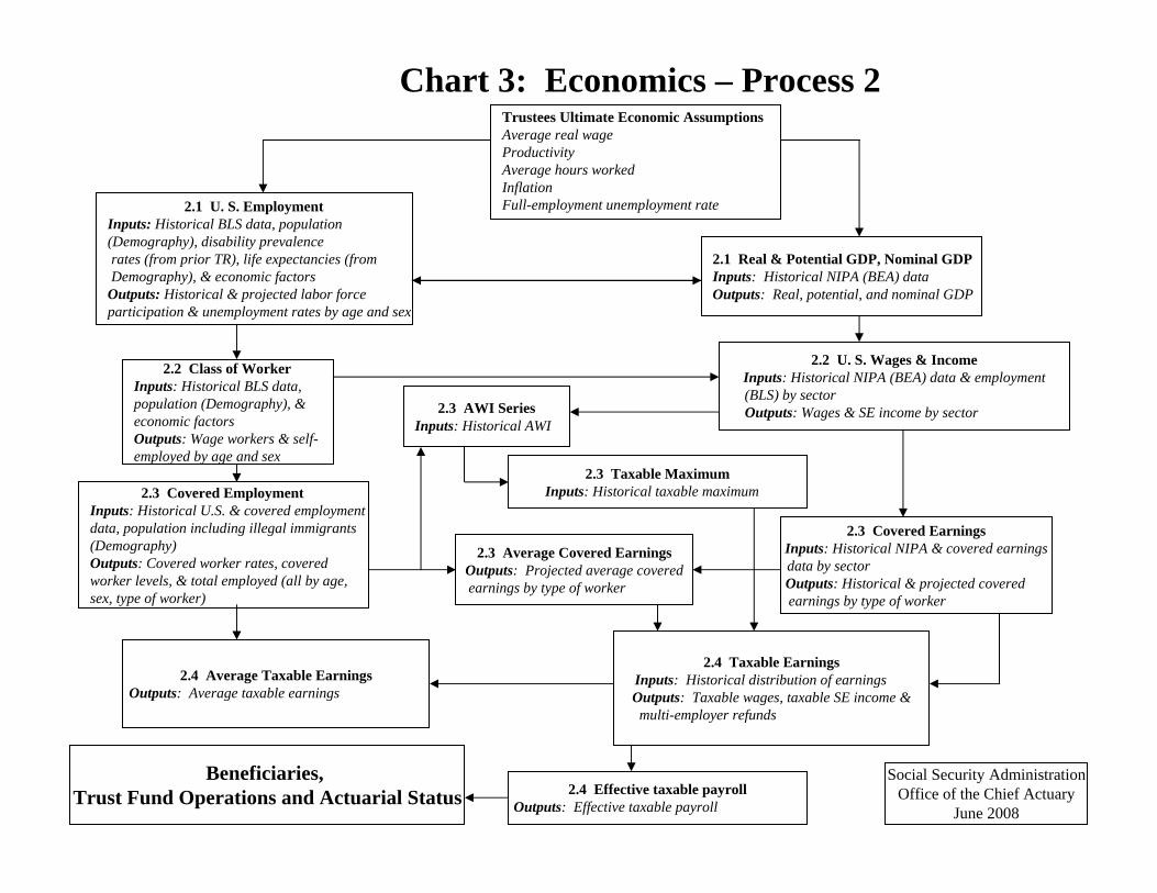
Trustees Ultimate Economic AssumptionsAverage real wageProductivityAverage hours workedInflationFull-employment unemployment rate

2.2 Class of WorkerInputs: Historical BLS data, population (Demography), & economic factorsOutputs: Wage workers & self-employed by age and sex

2.3 AWI SeriesInputs: Historical AWI

2.1 Real & Potential GDP, Nominal GDPInputs: Historical NIPA (BEA) dataOutputs: Real, potential, and nominal GDP

2.3 Covered EmploymentInputs: Historical U.S. & covered employmentdata, population including illegal immigrants (Demography) Outputs: Covered worker rates, covered worker levels, & total employed (all by age, sex, type of worker)

2.2 U. S. Wages & IncomeInputs: Historical NIPA (BEA) data & employment(BLS) by sector Outputs: Wages & SE income by sector

2.3 Average Covered EarningsOutputs: Projected average coveredearnings by type of worker

2.4 Taxable EarningsInputs: Historical distribution of earnings Outputs: Taxable wages, taxable SE income &multi-employer refunds

2.4 Average Taxable EarningsOutputs: Average taxable earnings

2.4 Effective taxable payrollOutputs: Effective taxable payroll

Chart 3: Economics – Process 2


June 2008

2.1 U. S. EmploymentInputs: Historical BLS data, population (Demography), disability prevalence rates (from prior TR), life expectancies (from Demography), & economic factors

Outputs: Historical & projected labor force participation & unemployment rates by age and sex

2.3 Covered EarningsInputs: Historical NIPA & covered earningsdata by sector Outputs: Historical & projected covered earnings by type of worker

Beneficiaries, Trust Fund Operations and Actuarial Status

2.3 Taxable MaximumInputs: Historical taxable maximum

3.1 Fully-insured (FI) populationInputs: Covered workers, median earnings,and AWI (Economics); SS area population (Demography); earnings distribution, historical FI population (historical and short-rangeprojections).Outputs: FI population (historical and projected)

3.1 Disability-insured (DII) populationInputs: Historical DII population Outputs: DII population (historical and projected)

3.2 Disabled-worker beneficiary (DIB) populationInputs: Base period incidence, recovery, and mortality rates. Projected Data -- Assumed ultimate changes in incidence rates, recovery rates, and mortality rates (Demography) from base period Outputs: DIB population and conversions to OAB (projected)

3.3 Old-Age beneficiary (OAB) populationInputs: Historical OAB population, labor force participation rates (Economics), and scheduled reductions for early retirement and increases fordelayed retirement Outputs: OAB population (projected)

3.3 Auxiliary Beneficiaries of Retired and Deceased WorkersInputs: Historical auxiliary beneficiaries of retired and deceasedworkers, SS area population by marital status (Demography), number of children with at least one retired parent (Demography),number of children with at least one deceased parent (Demography), average number of children per family (Demography) and other relationships Outputs: Auxiliary beneficiaries of retired and deceased workers by type of benefit (projected)


3.3 Widow beneficiary populationInputs: Historical widow beneficiary population,SS area population by marital status (Demography)and other relationshipsOutputs: Insured and uninsured widow beneficiarypopulation (projected)

Chart 4: Beneficiaries – Process 3


June 2008

3.2 DIB Auxiliary BeneficiariesInputs: Historical beneficiaries by type of benefit, Population (Demography), other relationships Outputs: Auxiliary beneficiaries of disabled workers by type of benefit (projected)

Note: Insured widow refers to widow beneficiaries who are insured for OAIB benefits, but not receiving those benefits

Trustees ultimate assumptionsDisability incidence rates Disability recovery rates Disability mortality rates

Chart 5: Trust Fund Operations and Actuarial Status – Process 4

4.3 Payroll taxesInputs: Payroll tax rate, effective taxable payroll (Economics), incurred-to-cash lag factor,short-range estimates Outputs: Payroll taxes

4.1 Fraction benefits taxableInputs: Historical and projected short-range data on income taxation of benefits from Office of Tax Analysisin the Department of the Treasury and data from current population survey Outputs: TOB as of a percent of benefits (projected)

4. 3 Taxation of benefits (TOB)Outputs: Taxes on benefits

4.3 Administrative expensesInputs: Short-range administrative expenses; total beneficiary population and AWI, assumed increase in productivity (Economics),Outputs: Administrative expenses

4.3 Benefit paymentsInputs: Starting average benefits, OAB population, DIB population,married and divorced aged population (Demography), Cost-of-Living Adjustments (Economics), post-entitlement factors, assumed benefit relationships between workers and auxiliaries, short-range estimates of benefit payments

Outputs: Scheduled benefit payments during year, average scheduledbenefits

4. 3 Railroad interchangeInputs: Data from Railroad Retirement Board and AWI, covered workers, taxable payroll (Economics), short range estimates of railroad interchange Outputs: Net payments to RRB

4. 3 Interest incomeInputs: Short-range estimatesof interest incomeOutputs: Interest income, annual yield rate on the OASI, DI, and combined funds

Trust Fund Operations and Actuarial StatusOutput: Summarized income and cost rates and actuarial balances; open Group unfunded obligations; annual income rate, cost rate and Balance: Dollar trust fund operations and trust fund ratiosSocial Security Administration

Office of the Chief ActuaryJune 2008

Trustees ultimate assumptionsReal interest rate, CPI

4.2 AIME Levels for newly-entitled OABs and DIBsInputs: Sample of newly-entitled OABs and DIBs; sampleof earnings from CWHS; SS area population (Demography);covered workers, average taxable earnings (Economics); and National Average Wage Index (AWI), Tax Maximum Outputs: Projected AIME distributions for new entitlements

1

II. Process Descriptions

The long-range programs used to make projections for the annual Trustees Report are grouped into four major processes. These include Demography, Economics, Beneficiaries, and Trust Fund Operations and Actuarial Status. Each major process consists of a number of subprocesses. Each subprocess is described in terms of three elements:

• This overview attempts to provide a general description of the purpose of each subprocess. Key projected variables used in the subprocess are introduced. Some variables are represented as being dependent in an equation, where the dependent variable is defined in terms of one or more independent variables. Independent variables may include previously calculated dependent variables or data provided from outside the subprocess. Other key variables are referenced by “(·)” following the variable name. This indicates that the calculation of this variable can not easily be communicated by an equation and, thus, requires a more complex discussion.

• Input Data – Data used in the subprocess are described. These data include those from

other subprocesses, ultimate long-range assumptions provided by the Board of Trustees of the OASDI Trust Funds, data from other offices of the Social Security Administration, and data from outside the Social Security Administration (e.g., estimates of the U.S. population). Data description includes data source and data detail (e.g., define age detail of data). In addition, an indication of how often additional data are expected to be received is included.

• Development of Output – The key variables are described in greater detail, including the

level of disaggregation of the data.

2

Process 1:

Demography

3

1. Demography

The primary purpose of the Demography Process is to provide estimates of the projected Social Security area population1 for each year of the 75-year projection period in the Trustees Report. For the 2008 report, the projection period covers the years 2008 through 2082. The Demography Process receives input data mainly from other government agencies and provides output data to the Economics, Beneficiaries, and Trust Fund Operations and Actuarial Status processes. The Demography Process is composed of seven subprocesses: FERTILITY, IMMIGRATION, MORTALITY, HISTORICAL POPULATION, MARRIAGE, DIVORCE, and PROJECTED POPULATION. As a rough overview, FERTILITY projects birth rates by age of mother, IMMIGRATION projects numbers of immigrants by age and sex, and MORTALITY projects probabilities of death by age and sex. HISTORICAL POPULATION combines population estimates from different sources to obtain historical estimates of the Social Security Area population by single year of age, sex and marital status. MARRIAGE projects marriage rates by age-of-wife crossed with age-of-husband and DIVORCE projects divorce rates by age-of-husband crossed with age-of-wife. PROJECTED POPULATION starts with the latest estimates of the Social Security Area population from HISTORICAL POPULATION and projects the population by age, sex, and marital status using projected values from FERTILITY, IMMIGRATION, MORTALIY, MARRIAGE, and DIVORCE. 1.1. FERTILITY 1.1.a. Overview The National Center for Heath Statistics (NCHS) collects data on annual numbers of births and the U.S. Census Bureau produces estimates of the resident population. Birth rates for historical years are calculated from these data by single year of age of mother. Age-specific birth rates ( z

xb ) for a given year z are defined as the ratio of (1) births ( zxB ) during the year to mothers at the

specified age x to (2) the midyear female population ( zxP ) at that age. The total fertility rate

zTFR summarizes the age-specific fertility rates for a given year. The total fertility rate for a given year z is defined as the sum of the age-specific birth rates for all ages x during the year z. It can be interpreted as the number of children born to a woman if she were to survive her

1 The Social Security area population consists of all persons who are potentially eligible to either receive benefits under the Social Security program or who have the potential to work in covered employment. This population consists of residents of the U.S. and its territories, citizens living abroad, and beneficiaries living abroad.

4

childbearing years and experience the age-specific fertility rates of year z throughout her childbearing years. The FERTILITY subprocess combines the historical values of z

xb and zTFR with an ultimate

assumed future value of the TFR to develop projections of zxb . The primary equations of this

subprocess are given below:

zxb = z

xb (.) (1.1.1)

∑=x

zx

z bTFR (1.1.2)

1.1.b. Input Data Trustees Assumptions -

Each year the Board of Trustees of the OASDI Trust Funds sets the ultimate assumed values for the TFR. The TFR reaches its ultimate value in the 25th year of the projection period. Under the intermediate assumptions underlying the 2008 Trustees Report, the ultimate TFR is 2.0 and it is assumed to be reached in 2032.

Other input data -

• From NCHS, annual numbers of births by age of mother2 (10-14, 15, 16, 17, …, 48, 49-54) for years 1980-2004. In general, NCHS provides an annual update including one additional year of birth data. The previous historical years are only updated if NCHS makes a historical revision to their data.

• From the U.S. Census Bureau, estimates of the July 1st female resident population by

single year of age for ages 14-49 for 1980-2004. Each year, Census provides updated data for years after the most recent decennial census

• NCHS historical birth rates, by single year of age of mother (14-49) for the period

1917-79. No updates of these data are needed. 1.1.c. Development of Output 2 The ages provided include 10-14, 15, 16, 17, …, 48, 49-54. Births at ages less than 14 are treated as having occurred at age 14 and ages reported to mothers older than 49 are treated as having occurred at age 49.

5

Equation 1.1.1 - Age-specific birth rates The FERTILITY subprocess produces the age-specific birth rates, by childbearing ages 14 through 49, for years 1941 through the 75-year projection period. For historical years prior to 1980, age-specific birth rates were obtained from NCHS. For years 1980 through the remaining

historical period, age-specific birth rates are calculated as: zx

zxz

x PB

b = , using birth data from NCHS

and estimates of the July 1st female resident population from the U.S. Census Bureau. The age-specific birth rates are projected using a process that is consistent with both the observed trends in recent data and the ultimate assumed total fertility rate. This process consists of the following steps:

1. Averaged birth rates by age group3, designated as zxb5 , are calculated from the age-

specific birth rates zxb for each year during the period 1979-2004.

2. To calculate the starting values of the projection process, the zxb5 from the last five years

of historical data are averaged using weights of 5, 4, 3, 2 and 1 for years 2004, 2003, 2002, 2001, and 2000 respectively.

3. For each zxb5 , the slope of the least squares line is calculated based on a regression over

the period 1979-2004.

4. For 2005, each of the seven starting values of zxb5 (from Step 2) is projected forward by

adding 100 percent of their respective slope (from Step3). Then, the total fertility rate, TFR z, is calculated such that it is equal to 5 times the sum of each z

xb5 . For the age group 14-49, 6 times the sum is included since this age group contains one additional age.

5. For the next year, 2006, the same calculation is done except each zxb5 for 2005 is

projected forward by adding 96 percent of the respective slope (from Step3). For subsequent projection years (2007-2032), an arithmetically decreasing portion4 is added to the previous year’s value of z

xb5 .

6. A preliminary total fertility rate, zpTFR , is calculated from the estimated values of z

xb5 (from Step 5) and is calculated in the same manner as Step 4.

3 The average is calculated by giving each age in the group equal weight without regard to population. The age groups calculated are 14-19, 20-24, 25-29, 30-34, 35-39, 40-44, and 45-49. 4 Each year of the projection the slope is reduced by four percentage points.

6

7. For years 2007 and later, an adjustment is made so that the annual TFR z is consistent with the Trustees’ assumed ultimate level5. For 2007, the TFR z is assumed to equal the level estimated for 2006 and then decrease linearly until reaching the ultimate value in 2032.

8. To ensure the assumed total fertility rate is achieved, each value of zxb5 (step 5) is

multiplied by the ratio of the assumed zTFR (step 7) and the respective value of TFRp (Step 6).

9. The final step of the projection method disaggregates the adjusted zxb5 into single age

birth rates by multiplying the zxb5 (Step 8) by the ratio of the single year z

xb to the zxb5

for each of the respective ages and age groups as calculated in the last year of complete historical data (Step 1).

1.2 MORTALITY 1.2.a. Overview The NCHS collects data on annual numbers of deaths and the U.S. Census Bureau produces estimates of the U.S. resident population. Central death rates (yMx) are defined as the ratio of (1) the annual number of deaths occurring during the year to persons between exact ages x and x+y to (2) the mid-year population between exact ages x and x+y. For historical years prior to 1968, yMx, are calculated from the NCHS and Census data by sex. For historical years after 1968, the same data are used in the calculations for ages under 65 but data from the Centers for Medicare and Medicaid Services (CMS) are used for ages 65 and over. Based on death by cause data from NCHS, the yMx, are distributed by cause of death for years 1979 and later6. Over the last century, death rates have decreased substantially. The historical improvement in mortality is quantified by calculating the average annual percentage reduction (yAAx) in the central death rate. In order to project future yMx, the Board of Trustees of the OASDI Trust

5 For 2005 and 2006, zTFR is assumed to equal z

pTFR .

6 Data needed in order to project central death rates by cause of death were obtained from Vital Statistics tabulations for years since 1979. For the years 1979-1998, adjustments were made to the distribution of the numbers of deaths by cause. The adjustments were needed in order to reflect the revision in the cause of death coding that occurred in 1999, making the data for the years 1979-1998 more comparable with the coding used for the years 1999 and later. The adjustments were based on comparability ratios published by the National Center for Health Statistics.

7

Funds determines the ultimate average annual percentage reduction that will be realized during the projection period ( u

xy AA ). The basic mortality outputs of the MORTALITY subprocess that are used in projecting the population are probabilities of death by age and sex (qx). The probability that a person age x will die within one year (qx) is calculated from the central death rates (the series of yMx). Period life expectancy ( ) is defined as the average number of years of life remaining for people who are age x and are assumed to experience the assumed probabilities of death throughout their lifetime. It is generated from the probabilities of death for a given year and is a summary statistic of overall mortality for that year. Age-adjusted death rates (ADR) are also used to summarize the mortality experience of a single year, making different years comparable to each other. Age-adjusted death rates are a weighted average of the yMx, where the weights used are the numbers of people in the corresponding age groups of the standard population, the 2000 U.S. Census resident population ( xy SP ). Thus, if the age-adjusted death rate for a particular year and sex is multiplied by the total 2000 U.S. Census resident population, the result gives the number of deaths that would have occurred in the 2000 U.S. Census resident population if the yMx for that particular year and sex had been experienced. Age-sex-adjusted death rates (ASDR) are calculated to summarize death rates for both sexes combined and are calculated as a weighted average of the yMx, where each weight is the number of people in the corresponding age and sex group of the 2000 U.S. Census resident population. MORTALITY projects annual yMx which are then used to calculate the program’s additional outputs. The equations for this subprocess, 1.2.1 through 1.2.6, are given below: yMx = yMx (·) (1.2.1) yAAx = yAAx (·) (1.2.2) qx = qx (·) (1.2.3)

8

= (·) (1.2.4)

∑∑ ⋅

=

xxy

zsxy

xxy

zs SP

MSPADR

,

(1.2.5)

∑∑∑∑ ⋅

=

s xsxy

s

zsxy

xsxy

z

SP

MSPASDR

,

,,

(1.2.6)

where zsxy M , refers to the central death rate between exact age x and x+y by sex in year z;

ySPx denotes the number of people in the standard population (male and female combined) who are between exact age x and x+y; and ySPx,s denotes the number of people by sex in the standard population who are between exact age x and x+y. 1.2.b. Input Data Trustees Assumptions -

Each year the Board of Trustees of the OASDI Trust Funds sets the ultimate assumed values for the yAAx by sex, age group7 and cause of death8. The average annual percentage reductions reach their ultimate value in the 25th year of the 75-year projection period. The ultimate rates of reduction by sex, age group, and cause of death can be found in Appendix 1.2-1.

NCHS Data -

• Annual numbers of registered deaths by sex and age group for the period 1900-1978. These data are not updated. Registered deaths refer to deaths in the Death Registration area. Since 1933, the Death Registration area has included all of the U.S.

• Annual numbers of deaths by sex, age group, and cause for the period 1979-2004.

Each year, a new year of data is generally received. In addition, revised data are often available for years beginning with 1999 (1999 was the starting year of the latest international classification of diseases – ICD10).

7 Age groups are: less than 15, 15-49, 50-64, 65-84, 85+ 8 The seven causes of death are: Heart Disease, Cancer , Vascular Disease, Violence, Respiratory Disease, Diabetes Mellitus, and Other

9

• The monthly number of births by sex for years 1938-2004. These data are updated annually, when NCHS provides an additional year of data.

• The number of infant deaths by age sex and age group9 for years 1938-2004. These

data are updated annually, when NCHS provides an additional year of data.

• Deaths for 1995 and 1996 by sex, 4 marital statuses, and 21 age groups. The age groups are generally 5-year age groups and are as follows: 0, 1-4, 5-9, 10-14, …., 95+). These data are updated as resources are available.

• The population of states in the Death Registration area by age group10 and sex for

years 1900-1939. These data are not updated.

• The number of registered deaths by sex and age groups (85-89, 90-94, and 95+) for the years 1900- 1967. These data are not updated.

U.S. Census Bureau Data -

• Estimates of the July 1 resident population by single year of age (0 through 100+) for years 1980-2004. Each year, Census provides an additional year of data and updated data for years after the most recent decennial census.

• From the Current Population Survey (CPS), the population by sex, marital status, and

age group11 for the years 1995 and 1996. These data are updated as resources are available.

• The resident population by sex, martial status, and age group12 as of as of July 1, 1995

and 1996. These data are updated when new NCHS death data by marital status are incorporated.

• The resident population by sex and age group13 for years 1900-1939. These data are

not updated. • The resident population at ages 75-79 and 80-84, by sex, for years 1900-1940 (at ten

9 Age groups are: under 23 hours, 1-2 days, 3-6 days, 7 -27 days, 28 days-1 month, 2 months, 3 months,…, 11 months 10 Age groups are: 0, 1-4, 5-14, 15-24, ..., 75-84, 85+ 11 Age groups are: 15-17, 18-19, 20-24, 25-29,..., 40-44, 45-54, ..., 65-74, and 85+ 12 Age groups are: 15-19, 20-24, 25-29, ..., 95+ 13 Age groups are: 0, 1-4, 5-14, 15-24, ..., 75-84, 85+

10

year intervals). These data are not updated. • The resident population by sex and age groups14 for 1940-2000. These data are not

updated.

Centers for Medicare and Medicaid Services Data -

• Annual numbers of deaths by sex and single year of age (ages 65 and over) for the period 1968-2004. These data are updated annually, when CMS provides an additional year of data.

• Annual numbers of Medicare enrollments (who are insured for Social Security

benefits) by sex and single year of age (ages 65 and over) for the period 1968-2004. These data are updated annually, when CMS provides an additional year of data.

Other input data -

• From the previous year’s Trustees Report the July 1, 1995 and 1996 Social Security

area population by sex, martial status, and single year of age (5 through 100+). These data are updated when new NCHS death data by marital status are incorporated.

1.2.c. Development of Output Equation 1.2.2 - Average Annual Percentage Reduction ( xy AA ) The xy AA by sex and cause are calculated based on the decline in the yMx for the period 1984 through 2004 and distributed by 21 age groups15, 2 sexes, and 7 causes of death16. The values are calculated as the complement of the exponential of the slope of the least-squares line through the logarithms of the yMx. The ultimate assumed values for the ( u

xy AA ), as set by the Board of Trustees of the OASI and DI Trust Funds, are assumed to be reached in the 25th year of the 75-year projection period. The assumed ultimate values are specified by sex, seven causes of death, and for the following five age groups: under age 15, 15-49, 50-64, and 65-84, and 85 and older.

14 Age groups for years prior to 1980 are: 0, 1-4, 5-9, ..., 85+. For years 1980-1982, the age groups are: 0, 1-4, 5-9, ..., 95+. For years 1983 and later, the age groups are 0, 1-4, 5-9, ..., 85+. 15 Age groups are: 0, 1-4, 5-9, 10-14, ……, 90-95, and 95+ 16 The seven causes of death are: Heart Disease, Vascular Disease, Violence, Cancer, Respiratory Disease, Diabetes Mellitus, and Other.

11

The values of xy AA by the 21 age groups, sex, and cause for 2005 through 2007 are assumed to equal the average xy AA based on the decline in the yMx for the period 1984-2004. If, however, the average xy AA for a particular group during the period is negative, then 75 percent of the average rate is used. For years after 2007, a method of graduation is used that causes the absolute difference between the current xy AA and the ultimate u

xy AA to decrease rapidly until it

reaches the Trustees’ ultimate assumed value, uxy AA . This is accomplished by repeating the

following steps for each year of the projection:

1. The absolute value of the distance between the prior year’s calculated xy AA and the

ultimate assumed uxy AA is calculated.

2. If the ultimate assumed uxy AA is greater than the prior year’s xy AA , 80 percent of the

difference is subtracted from the ultimate assumed uxy AA . If the ultimate assumed

uxy AA is less than the prior year’s xy AA , then 80 percent of the difference is added to

the ultimate assumed uxy AA .

3. These steps are repeated until the 25th year at which time the xy AA are set equal to their ultimate assumed values.

Equation 1.2.1 – Central Death Rates (yMx)

Values of yMx are determined for each historical and projected year by the 21 age groups, 2 sexes, and 7 causes of death. The starting year for the projections of the yMx is 2004, and is the most recent data year in the historical period. However, instead of using the historical data for yMx in this year as the starting point for mortality projections, starting yMx are calculated to be consistent with the trend inherent in the last 12 years of available data. Each starting value for the yMx, by sex and cause of death, is computed as the value for the most recent year falling on a weighted least square line, where yMx is regressed on year, over the last 12 years. The weights are 0.2, 0.4, 0.6, and 0.8 for the earlier four years of the 12 years and are 1.0 for all other years.

For years after 2004, yMx are projected by sex and cause of death by applying the respective xy AA to the prior year yMx.

Equations 1.2.3 – Probabilities of death (qx)

12

In order to project population by age and sex, probabilities of death are applied to determine the projected number of deaths that will occur in the population. These probabilities, denoted as qx, reflect the probability a person age x will die within one year, where x refers to age last birthday as of the beginning of each year. For each year in the historical and projection period, separate qx, series are estimated by sex. Different methods of projecting qx are used for age 0, for ages 1 through 4, for ages 5 through 95 and for ages 95 and above. The following descriptions provide a brief discussion of these different methods. Additional detail is provided in Actuarial Study number 120 located at the following internet site: http://www.socialsecurity.gov/OACT/NOTES/as120/LifeTables_Foreword.html.

• Values for qx at Age 0: During the first year of life, mortality starts at an extremely high level, which becomes progressively lower, unlike mortality at other ages which does not change very much within a single year of age. Thus, it is particularly important at age 0 to estimate accurately the pattern of mortality throughout the year of age, as described above, for the calculation of q0. For the period 1940 through the last historical year, q0 is calculated directly from tabulations of births by month and from tabulations of deaths at ages 0, 1-2, 3-6, 7-28 days, 1 month, 2 months, ..., 11 months. After the last historical year, q0 is calculated from 1M0, assuming that the ratio of q0 to 1M0 measured for the last historical year would remain constant thereafter.

• Values for qx at Ages 1 – 4: For the period 1940 through the last year of historical data, probabilities of death at each age 1 through 4 (qx, x = 1, 2, 3, 4) are calculated from tabulations of births by year and from tabulations of deaths at ages 1, 2, 3, and 4 years. After the last historical year, each qx (where x = 1, 2, 3, 4) is calculated from 4M1 assuming that the ratio of qx to 4M1 measured for the last historical year would remain constant thereafter.

• Values for qx at Ages 5 – 94: Probabilities of death for these ages are calculated from the

projected central death rates, 5Mx. As mentioned above, the calculations are discussed in detail in Actuarial Study number 120.

• Values for qx at Ages 95+: It has been observed that the mortality rates of women, though lower than those of men, tend to increase faster with advancing age than those of men. An analysis of Social Security charter Old-Age Insurance beneficiaries has shown that at the very old ages mortality increases about five percent per year of age for men and about six percent per year for women. Probabilities of death at each age 95 and older are calculated as follows for men:

13

For women, the same formulas are used, except that 1.06 is substituted for 1.05. The larger rate of growth in female mortality would eventually, at a very high age, cause female mortality to be higher than male mortality. At the point where this crossover would occur, female mortality is set equal to male mortality.

The values of qx used in projecting the population are based on age last birthday and are calculated by sex for 1/2q0 and for qx where x represents age last birthday and equals 0, 1, 2, ….., 99. Because life table values of probabilities of death are based on exact ages, values for qx representing age last birthday for ages 0 through 99 are derived by averaging the life table values of probabilities of death at ages x and x+1. Deaths occurring during the first six months of life are calculated directly from the life tables’ values and are applied to births during the year. Deaths occurring in the population at ages 100 and older are projected as a group. In addition, probabilities of death are broken down further into marital status. Historical data indicate differential in mortality by marital status is significant. To reflect this, projected relative differences in death rates by marital status are projected to be the same as observed during calendar years 1995 and 1996. Equation 1.2.4 –Life expectancy Actuarial Study number 120 presents background information on the calculation of life expectancy, from the probabilities of death (qx,). This study, titled Life Tables for the United States Social Security Area 1900-2100, can be accessed at the following internet site: http://www.socialsecurity.gov/OACT/NOTES/as120/LifeTables_Foreword.html. 1.3. IMMIGRATION 1.3.a. Overview Immigration consists of legal immigration, legal emigration, other immigration and other emigration. Legal immigration is defined as those persons who have been admitted into the United States and been granted legal permanent resident (LPR) status. Legal emigration consists of legal permanent residents and U.S. Citizens who depart the Social Security area population to reside elsewhere. Other immigrants include persons, other than LPRs, who enter the U.S. and

14

reside for 6 months or longer such as undocumented immigrants, temporary workers, and foreign students. Other emigration includes other immigrants who depart the Social Security area for another country in addition to those who adjust status to become an LPR. For each year z of the projection period, the IMMIGRATION subprocess produces estimates of legal immigration (Lz), legal emigration (Ez), and other immigration (Oz), by age and sex, based on assumptions set by the Trustees for each category. Estimates of other emigration are not developed in this subprocess, but rather are developed in the projected population subprocess documented in section 1.7. In addition, the IMMIGRATION subprocess disaggregates the estimates of Lz into those who have been admitted into the United States during the year (NEWz) and those who adjusted from the other-immigrant population to LPR status (AOSz) Each fiscal year17, the Department of Homeland Security (DHS) collects data on the number of persons granted LPR status by age, sex, and class of admission. The U.S Census Bureau provided OCACT with an unpublished estimate of the annual number of legal emigrants, by sex and age, based on the change between the 1980 and 1990 census. The Census Bureau also estimated the aggregate number of net other immigrants who entered the country during 1975-1980, by age and sex. These historical data are used as a basis for developing age-sex distributions that are applied to the Trustees’ aggregate immigration assumptions to produce annual immigration and emigration estimates by age and sex.

The primary equations of IMMIGRATION, by age (x) and sex(s), for each year (z) of the 75-year projection period are summarized below:

)(,, ⋅= zsx

zsx NEWNEW (1.3.1)

)(,, ⋅= zsx

zsx AOSAOS (1.3.2)

zsx

zsx

zsx AOSNEWL ,,, += (1.3.3)

)(,, ⋅= zsx

zsx EE (1.3.4)

zsx

zsx

zsx ELNL ,,, −= (1.3.5)

)(,, ⋅= zsx

zsx OO (1.3.6)

1.3.b. Input Data Trustees Assumptions - Each year the Board of Trustees of the OASDI Trust Funds specifies the total annual assumed values for legal immigration, legal emigration, and other immigration. For the 2008 Trustees

17 The federal fiscal year begins on October 1 and ends on September 30 of the next calendar year.

15

Report, the ultimate values for legal immigration and emigration are 1,000,000 and 250,000 respectively (both reached in 2010). For other immigration, the Trustees set the annual level at 1,500,000 persons per year for each year of the projection period.

Other input data -

• Historical legal immigration from DHS by fiscal year (1996-2006), single year of age (0 through 84), sex, and class of admission (New Arrival, Adjustment of Status, Refugee, and Asylee). This data is updated annually, with DHS providing an additional year of data each year.

• Unpublished estimates of annual legal emigration from The U.S Census Bureau by five-

year age groups (0-4, 5-9,…, 80-84) and sex based on the change between the 1980 and 1990 census. These data are updated occasionally (based on having new data from an outside source and on OCACT resource time constraints).

• Legal emigration conversion factors. These estimates were developed internally by five-

year age groups (0-4, 5-9,…, 80-84) and sex to reflect the fact that the estimated number of people leaving the United States is not equivalent to the number of people leaving the Social Security Area. These data are updated when annual legal emigration estimates are updated (see above).

• Unpublished tabulations from the U.S Census Bureau of the cumulative number net other

immigrants entering the country during 1975-1980 by five-year age groups (0-4, 5-9,…, 80-84) and sex. These data are updated occasionally (based on having new data from an outside source and on OCACT resource time constraints).

1.3.c. Development of Output Equations 1.3.1 and 1.3.2 – Legal Immigration The Trustees specify the aggregate amount of legal immigration for each year of the 75-year projection period. In order to incorporate the numbers of new immigrants into the Social Security area population projections, the total level of new immigrants is disaggregated by age and sex. There are two ways for an immigrant to be admitted into the U.S. for lawful permanent residence:

(1) New arrivals such as persons living abroad who are granted an LPR visa and then enter the U.S. through a port of entry. Refugees and asylees that are granted LPR status are also treated as new arrivals in the OCACT model.

16

(2) Adjustments of status, who are people already residing in the U.S. as other immigrants

and have an application for adjustment to LPR status approved by DHS.

The DHS provides data on legal immigrants by sex, single year of age, classification of admission, and fiscal year of entry. The 10 most recent years of data are used to calculate separate age-sex distributions for both new arrivals and adjustments of status by taking the following steps:

1. The data for the last ten years of single-year of age data are combined into five-year age groups.

2. Refugee and Asylee LPR admissions are subtracted from the adjustment of status data and added into the new arrival category.

3. The data are converted from fiscal year data to calendar year data. 4. For each class of admission, new arrival and adjustment of status, the historical data for

the last 10 years (from 1997-2006) are combined into an average age-sex distribution. 5. The distributions by five year age group are disaggregated into a single year of age-sex

distribution using the H.S. Beers method of interpolation.

Based on trends in the historical data, it is assumed that fifty percent of all new LPR admissions will be new arrivals and the other fifty percent will consist of adjustments of status. Thus,

zsxNEW , , the expected number of new arrival legal immigrants by age (x) and sex (s), is

calculated by applying the age-sex distribution for new arrivals to one half of the Trustees assumed level of legal immigration. The remaining half of the Trustees’ assumed number of legal immigrants is multiplied by the age-sex distribution of adjustments of status to calculate z

sxAOS , . Equation 1.3.4 – Legal Emigration The Trustees specify the aggregate amount of legal emigration for each year of the projection period. This is done by setting the ratio of emigration to legal immigration. For the 2008 Trustees Report, the ratio is set at 25 percent. In order to produce the number of emigrants from the Social Security area population, the total level of emigrants is disaggregated by age and sex. The disaggregation is based on a distribution of emigrants, by sex and five-year age groups, provided to OCACT in unpublished estimates by Census that are based on changes between the 1980 and 1990 census. Since the emigration numbers estimated by Census are for all people leaving the United States, they are adjusted downward by a series of conversion factors so the data correspond to the number of people leaving the Social Security area population.

17

For each sex, the Beers formula is used to interpolate and distribute each five-year age group into a single year of age-sex distribution, EDISTx,s. For each projection year, this distribution is used to distribute the assumed level of total legal emigrants by age and sex using the following equation:

∑∑= =

=f

ms xsxsx

zsx EDISTLE

84

0,,, *)(25.

Equation 1.3.6 – Other Immigration The term “other immigration” refers to persons entering the U.S. in a manner other than being lawfully admitted for permanent residence. This includes temporary immigrants (persons legally admitted for a limited period of time) in addition to undocumented immigrants living in the U.S. The Trustees specify the aggregate amount of other immigrants for each year of the projection period. For each projection year, an age-sex distribution is used to distribute this assumption by age and sex. This age-sex distributions is denoted as ODISTx,s and is developed from a weighted average of the distribution of adjustments of status from Equation 1.3.2 and an age-sex distribution of non-adjusting other immigrants. The age distribution of the adjustments of status is modified to incorporate a five year set back based on the assumption that adjustments of status enter the U.S. five years earlier on average. This age-sex distribution is denoted as ODIST1x,s. The age distribution of non-adjusting other immigrants, ODIST2x,s is derived from an unpublished census estimate of net other immigration during the period 1975-80 using assumed levels of persistence. The two age distributions are then combined using the following formula:

sxsxsx ODISTwODISTwODIST ,,, 2)1()1( −+= Where w is a weighting factor equal to the Trustees ultimate assumed level of adjustments of status increased by a factor18 of 1.25 divided by the Trustees ultimate assumed level of other immigration. For the 2008 Trustees Report, this w equals 0.625. Thus, for each year (z) other immigration is defined by the following equation:

sxz

sx ODISTO ,, 000,500,1 ∗= 1.4. HISTORICAL POPULATION 18 This factor is meant to take into account that a large number of people who have the potential to adjust to LPR status may die or return to their native country prior to doing so.

18

1.4.a Overview For each historical year, the HISTORICAL subprocess provides estimates of the Social Security area population by for the period 1941 through 2006. The Social Security area population consists of:

• U.S. resident population and armed forces overseas plus • Net census undercount plus • Civilian residents of Puerto Rico, the Virgin Islands, Guam, the Northern Mariana

Islands, and American Samoa plus • Federal civilian employees overseas plus • Dependents of armed forces and federal civilian employees overseas plus • Residual beneficiaries living abroad plus • Other citizens overseas

The U.S. Census Bureau collects population data and tabulates it by age, sex, and marital status every ten years for the decennial census. The decennial census includes data from the 50 states, the District of Columbia, U.S. territories and citizens living abroad. Each subsequent year, the Census Bureau publishes an estimate of the post-censal population. This subprocess combines these censal estimates, along with the estimates of the other components of the Social Security area population listed above and components of change described in sections 1.1 to 1.3 to develop smoothed estimates of the Social Security area population by single year of age and sex ( z

sxP , ). Combining this population with an estimated marital status matrix provides the Social

Security area population by single year of age, sex, and marital status ( zmsxP ,, ). These estimates

are then used as the basis for the POPULATION PROJECTION process described in section 1.7. The primary equations for this subprocess, 1.4.1 and 1.4.2 are given below:

zsxP , = z

sxP , (·) (1.4.1)

zmsxP ,, = z

msxP ,, (·) (1.4.2) 1.4.b. Input Data Long-Range OASDI Projection Data -

Demography • Probabilities of death from MORTALITY, by age last birthday and sex, for years

1941-2005. These data are updated every year.

19

• The number of new legal immigrants by age and sex for years 1941-2005. These

data are from the IMMIGRATION subprocess and are updated each year. U.S. Census Bureau Data -

• Decennial census total population estimates. A new estimate is available every ten

years. • Estimates of U.S resident population and Armed Forces population overseas as of

each July 1 (1980-2006) by sex and single-year of age 0 through 99, and ages 100 and older. Each year, the U.S. Census Bureau restates the data back to the most recent decennial census and includes one additional year of data.

• Estimates of the 1940, 1950, and 1960 counts of the U.S. population and armed

forces overseas by sex and single year of age (0-84) and the age group 85+. These data are not updated.

• Estimates of the population by age group19, sex, and marital status for years 1940-

2006. An additional year of data is added for each Trustees Report. • Estimates of the population by marital status, which have more age groups than the

CPS, and sex for years 1982-1989 and 1992-2000. These data are not updated. • Undercount factors by single year of age (0-85+) and sex, estimated using post-

censal survey data. These data are updated after each decennial census. • The total annual civilian population estimates for Puerto Rico, Virgin Islands,

Guam, Northern Marianas, and American Samoa for years 1940-2006. For each Trustees Report, an additional data year is downloaded from the U.S. Census Bureau’s international database.

• Estimates of U.S resident population and Armed Forces population overseas as of

each July 1 (1940-1979) by sex and single-year of age through 84, and for the group aged 85 and older. These data are not updated.

• From the U.S. Census Bureau 1980 Census of Population, Subject Report on

Marital Status No. PC80-2-4C, number of existing marriages in 1980 by age group of husband crossed with age group of wife. These data are not updated.

19 Age groups are: 15-17, 18-19, 20-24, 25-29, ..., 55-64, 65-74, 75-84, 85+

20

Other input data -

• From the Centers for Medicare and Medicaid (CMS), the population insured for Social Security benefits by single year of age (85-100+) and sex for years 1968-2006. The last year of data is provisional. Each year, CMS provides a final year of data to replace the prior year’s provisional data and a new provisional year of data.

• The SSA Annual Statistical Supplement provides estimates of the total number of

OASDI Beneficiaries living abroad for years 1987-2006. For each Trustees Report, an additional year of data is available.

• Output from the Urban Institute’s microsimulation model, POLISIM, regarding

marriage prevalence for the period 1980-2006 by age of husband and age of wife. For each Trustees Report, the data may be revised and an additional year of data may be added.

1.4.c. Development of Output Equation 1.4.1 – Historical Population by age and sex ( z

sxP , ) The Census Bureau's estimate of the residents of the 50 States, D.C., and U.S. Armed Forces overseas is used as a basis for calculating z

sxP , . The base estimate is adjusted for net census undercount and increased for other U.S. citizens living abroad (including residents of US territories) and for non-citizens living abroad who are insured for Social Security benefits. The estimates of the number of residents of the fifty States and D.C. and Armed Forces overseas, as of July 1 of each year, by sex for single years of age through 84, and for the group aged 85 or older, are obtained from the Census Bureau. Adjustments for net census undercount are estimated using post-censal survey data from the Bureau of the Census. The numbers of persons in the other components of the Social Security Area as of July 1 are estimated by sex for single years of age through 84, and for the group aged 85 or older, from data of varying detail. Numbers of civilian residents of Puerto Rico, the Virgin Islands, Guam, American Samoa, and the Northern Mariana Islands are estimated from data obtained from the Bureau of the Census. Numbers of Federal civilian employees overseas, dependents of these Federal civilian employees, dependents of Armed Forces overseas, and other citizens overseas covered by Social Security are also based on estimates used by the Bureau of Census. The overlap among the components, believed to be small, is ignored.

21

The first step of the process is to estimate zsxP , as of January 1st for each decennial census year

and the last year of historical data (2006 for the 2008 Trustees Report). For ages 0-84, zsxP , is set

equal to the estimate from the decennial Census plus the undercount adjustment and other component populations. The decennial census estimates are as of April 1 but are converted to a January 1st population based on the surrounding applicable intercensal July20 population estimates. The population for final historical year is estimated based on the surrounding post-censal July populations. For ages 85 and over, data from the Center for Medicare and Medicaid Statistics (CMS) are used to distribute the population into single-year of age. For years between the decennial census years and years between the 2000 census and the last historical data year, populations are estimated taking into account the components of changes due to births, deaths, and legal immigration during that time period. These intercensal estimates are then multiplied by the appropriate age-sex-specific ratios so that the error of closure at the decennial census years is eliminated. Equation 1.4.2 – Historical Population by age, sex, and marital status ( z

msxP ,, ) Since eligibility for auxiliary benefits is dependent on marital status, the Social Security area population is disaggregated by marital status. The four marital states are defined as single (having never been married), married, widowed, and divorced. The distribution of the number of existing marriages is based on the 1980 Census Marital Status Report, which contains the number married couples in 1980 by age group of husband crossed with age group of wife. Additional tabulations from the POLISM model for 1980 through 2006 are incorporated to adjust these marital prevalence grids for changes since 1980. Multiplying the previous year values by the ratio the current year POLISM value to the previous year POLISM value ensures that the 1980 and later grids are consistent with the pre-1980 grids. The grids are transformed from age grouped numbers to single year of age figures from ages 14 to 100+ for husband and wife using the two dimensional H.S. Beers method of interpolation. Percentages of single, married, widowed, and divorced persons are calculated by taking the estimate for each marital status category and dividing them by the total number of people for each age group and sex from either the CPS or the more detailed Census numbers if available. Then, for each sex, if one age group has a higher or lower percentage than the surrounding age groups, an average of the surrounding groups replaces the original value. These percentages are multiplied by the total populations calculated in Equation 1.4.1 for each age, sex, and year to get a preliminary population for each age, sex, and marital status.

20 For years prior to decennial years 1960 and earlier the April 1 population estimates are used.

22

To keep the marriage prevalence grids and the marital status percentages smooth, several smoothing algorithms are used. First, the married population is adjusted so that the number of married males equals the number of married females. Next, the marital prevalence grids are smoothed so that each age of husband crossed with age of wife cell is an average of values in its diagonal in the grid. Finally, the number of married persons for each age and sex is set equal to the marginal total of the associated year’s marital prevalence grid. 1.5. MARRIAGE 1.5.a Overview The National Center for Heath Statistics (NCHS) collected detailed data on the annual number of new marriages in the Marriage Registration area (MRA), by age of husband crossed with age of wife, for the period 1978 through 1988 (excluding 1980). In 1988, the MRA consisted of 42 States and D.C. and accounted for 80 percent of all marriages in the U.S. Estimates of the unmarried population in the MRA were obtained from NCHS by age and sex. Marriage rates for this period are calculated from these data. NCHS stopped collecting data on the annual number of new marriages in the MRA in 1989. Less detailed data on new marriages from a subset of the MRA were obtained for the years 1989-1995. These data are used to determine marriage rates by adjusting the more detailed age-of-husband crossed with age-of-wife data from the earlier years to match the aggregated levels for these years. Age-specific marriage rates ( z

yxm ,ˆ ) for a given year z are defined as the ratio of (1) number of marriages for given age-of-husband (x) crossed with age-of-wife (y) to (2) a theoretical midyear unmarried population at that age ( z

yxP , ). The theoretical midyear population is defined as the geometric mean21 of the midyear unmarried males and unmarried females.

21 The square root of the product of the midyear unmarried male and unmarried female populations.

23

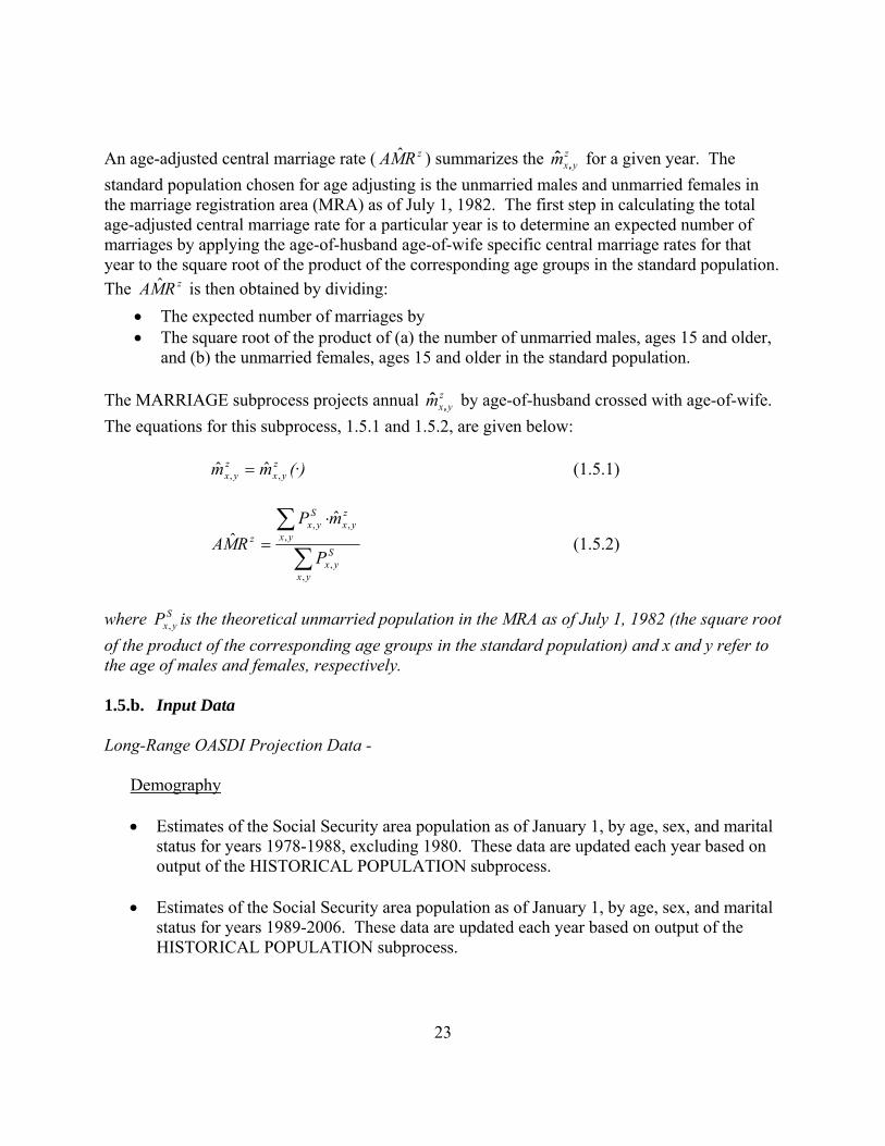
An age-adjusted central marriage rate ( zRMA ˆ ) summarizes the zyxm ,ˆ for a given year. The

standard population chosen for age adjusting is the unmarried males and unmarried females in the marriage registration area (MRA) as of July 1, 1982. The first step in calculating the total age-adjusted central marriage rate for a particular year is to determine an expected number of marriages by applying the age-of-husband age-of-wife specific central marriage rates for that year to the square root of the product of the corresponding age groups in the standard population. The zRMA ˆ is then obtained by dividing:

• The expected number of marriages by • The square root of the product of (a) the number of unmarried males, ages 15 and older,

and (b) the unmarried females, ages 15 and older in the standard population. The MARRIAGE subprocess projects annual z

yxm ,ˆ by age-of-husband crossed with age-of-wife. The equations for this subprocess, 1.5.1 and 1.5.2, are given below:

zyx

zyx mm ,, ˆˆ = (·) (1.5.1)

∑∑ ⋅

=

yx

Syx

zyx

yx

Syx

z

P

mPRMA

,,

,,

, ˆˆ (1.5.2)

where S

yxP , is the theoretical unmarried population in the MRA as of July 1, 1982 (the square root of the product of the corresponding age groups in the standard population) and x and y refer to the age of males and females, respectively. 1.5.b. Input Data Long-Range OASDI Projection Data -

Demography • Estimates of the Social Security area population as of January 1, by age, sex, and marital

status for years 1978-1988, excluding 1980. These data are updated each year based on output of the HISTORICAL POPULATION subprocess.

• Estimates of the Social Security area population as of January 1, by age, sex, and marital

status for years 1989-2006. These data are updated each year based on output of the HISTORICAL POPULATION subprocess.

24

Assumptions - For each Trustees Report ultimate values for the zRMA ˆ are assumed. The zRMA ˆ reaches its ultimate value in the 25th year of the 75-year projection period. For 2008, the intermediate ultimate zRMA ˆ assumption is 4,000 per 100,000 unmarried couples.

NCHS Data -

• Number of new marriages in the MRA, by age-of-husband crossed with age-of-wife, for calendar years 1978 through 1988, excluding 1980. These data are no longer available for years after 1988. The data vary in detail by year. They are broken out by single year age-of-husband crossed with single year age-of-wife for many ages (particularly younger ages).

• Number of unmarried males and females in the MRA for calendar years 1978 through

1988, excluding 1980. These data are no longer available for years after 1988. The data are generally broken out by single year age for ages under 40 and by age groups 40-44, 45-49, 50-54, 55-59, 60-64, 65-74, and 75+.

• Number of new marriages, in a subset of the MRA, by age-group-of-husband crossed

with age-group-of-wife (age groups include 15-19, 20-24, 25-29, 30-34, 35-44, 45-54, 55-64, and 65+), for calendar years 1989-1995. These data are updated as data becomes available and internal resources are sufficient to examine and interpret such new data.

• The total number of marriages in the United States for the period 1978-2006. Each year,

NCHS publishes the total number of marriages for a more recent year.

• Number of marriages in the MRA for years 1979 and 1981-1988 by age group (age groups include 14-19, 20-24, 25-29, 30-34, 35-44, 45-54, 55-64, and 65+), sex, and prior marital status (single, widowed, and divorced). These data are no longer available for years after 1988.

• Number of unmarried people in the MRA for years 1979 and 1981-1988 by age group

(age groups include 14-19, 20-24, 25-29, 30-34, 35-44, 45-54, 55-64, and 65+), sex, and prior marital status (single, widowed, and divorced). These data are no longer available for years after 1988.

1.5.c. Development of Output Equation 1.5.1 -

25

Age-specific marriage rates are determined for a given age-of-husband crossed with age-of-wife, where ages range from 14 through 100+. The historical period includes years of complete NCHS data on the number of marriages and the unmarried population in the Marriage Registration Area (MRA) for the period 1978 through 1988, excluding 1980. Provisional data are used for the period 1989 through 1995 and total number of marriages is used for the period 1996 through 2006. The projection period of the MARRIAGE subprocess begins one year after the last historical data year. The historical age-specific marriage rates are calculated for each year in the historical period based on NCHS data of the number of new marriages by age-of-husband crossed with age-of-wife and the number of unmarried persons by age and sex. The formula use in the calculations is given below:

zyx

zyxz

yx PM

m,

,,

ˆˆ = , where

• zyxM ,

ˆ is the number of marriages in year z;

• ( zyxP , ) is the geometric mean22 of the midyear unmarried males and unmarried females

in year z; and • x refers to age of males and y refers to the age of females.

The rates for the period 1978 through 198823 are then averaged, graduated, and loaded into an 87 by 87 matrix (age-of-husband crossed with age-of-wife for ages 14 through 100+), denoted as MarGrid. This matrix is used in the calculation of the age-specific marriage rates for all later provisional years and the years in the projection period. For the first part of the provisional period, 1989-1995, NCHS provided data on the number of marriages in a subset of the MRA by age-group-of-husband crossed with age-group-of-wife (age groups include 15-19, 20-24, 25-29, 30-34, 35-44, 45-54, 55-64, and 65+). These data are used to change the distribution of MarGrid by these age groups. For each age-group-of-husband crossed with age-group-of-wife, the more detailed marriage rates in MarGrid that are contained within this group are adjusted so that the number of marriages obtained by using the rates in MarGrid match the number implied by the MRA subset. For each year of the provisional period, an expected total number of marriages is calculated by multiplying the rates in the MarGrid (or the adjusted MarGrid for years 1989-1995) by the corresponding geometric mean of the unmarried males and unmarried females in the Social Security area population. All rates in MarGrid (or the adjusted MarGrid for years 1989-1995)

22 The square root of the product of the midyear unmarried male and unmarried female populations. 23 Data for 1980 is not available and excluded from the calculations.

26

are then proportionally adjusted to correspond to the total number of marriages estimated in the year for the Social Security area population. This estimate is obtained by increasing the number of marriages reported in the U.S. to reflect the difference between the Social Security area population and the U.S. population. The provisional age-specific rates are then graduated using the Whittaker-Henderson method and are used to calculate the age-adjusted rates for each year. The age-adjusted marriage rates are expected to reach their ultimate value in the 25th year of the 75-year projection period. Rather than use the last year of provisional data to calculate the starting rate, the rates for the past five years are averaged to derive the starting value. The annual rate of change in the age-adjusted marriage rate is calculated by taking the 26th root of the ratio of the ultimate value and the starting value. Thus, to calculate the rate for a projected year, the rate of change is applied to the prior year’s rate (or the starting value for the first year of the projection period). To obtain the age-of-husband-age-of-wife-specific rates for a particular year from the age-adjusted rate projected for that year, the age-of-husband-age-of-wife-specific rates in MarGrid are proportionally scaled so as to produce the age-adjusted rate for the particular year. A complete projection of age-of-husband-age-of-wife-specific marriage rates was not done separately for each previous marital status. However, experience data indicate that the differential in marriage rates by prior marital status is significant. Thus, future relative differences in marriage rates by prior marital status are assumed to be the same as the average of those experienced during 1979 and 1981-1988. 1.6. DIVORCE 1.6.a. Overview For the period 1979 through 1988, the National Center for Heath Statistics (NCHS) collected data on the annual number of divorces in the Divorce Registration area (DRA), by age-group-of-husband crossed with age-group-of-wife. In 1988, the DRA consisted of 31 States and accounted for about 48 percent of all divorces in the U.S. These data are then inflated to represent an estimate of the total number of divorces in the Social Security area. This estimate for the Social Security Area is based on the total number of divorces during the corresponding calendar year in the 50 States, the District of Columbia, Puerto Rico, and the Virgin Islands. Divorce rates for this period are calculated using this adjusted data on number of divorces and estimates of the married population by age and sex in the Social Security Area. An age-of-husband crossed with age-of-wife specific divorce rate ( z

yxd ,ˆ ) for a given year z is

defined as the ratio of (1) the number of divorces in the Social Security area for the given age of

27

husband and wife ( zyxD ,

ˆ ) to (2) the corresponding number of married couples in the Social

Security area ( zyxP , ) with the given age of husband (x) and wife (y). An age-adjusted central

divorce rate ( zyxRDA ,

ˆ ) summarizes the zyxd ,

ˆ for a given year. The zRDA ˆ is calculated by determining the expected number of divorces by applying:

• The age-of-husband crossed with age-of-wife specific divorce rates to • The July 1, 1982 population of married couples in the Social Security area by

corresponding age-of-husband and age-of-wife. The expected number of divorces is then divided by the total number of married couples in that year. The DIVORCE subprocess projects annual z

yxd ,ˆ by age-of-husband crossed with age-of-wife.

The primary equations, 1.6.1 and 1.6.2, are given below:

zyx

zyx dd ,,

ˆˆ = (·) (1.6.1)

∑∑ ⋅

=

yx

Syx

zyx

yx

Syx

z

P

dPRDA

,,

,,

,ˆ

ˆ (1.6.2)

where S

yxP , is the number of married couples in the Social Security area population as of July 1, 1982 and x and y refer to the age of husband and age of wife, respectively. 1.6.b. Input Data Long-Range OASDI Projection Data -

Demography • Social Security area population of married couples by age-of-husband crossed with age-

of-wife as of January 1 for years 1979-2006. These data are updated each year from the HISTORICAL POPULATION subprocess.

• Social Security area population of married couples by age-of-husband crossed with age-

of-wife for some projected years. These data are updated each year from PROJECTED

28

POPULATION subprocess of the prior year’s Trustees Report.

• The total population in the Social Security area for years 1979-2006. An additional year of data is added each Trustees Report.

Assumptions -

Each year the ultimate assumed value for the age-adjusted divorce rate is established. The rate reaches its ultimate value in the 25th year of the 75-year projection period. For 2008, the ultimate assumed zRDA ˆ is 2,000 per 100,000 married couples.

NCHS Data -

• The number of divorces in the divorce registration area (DRA), by age-of-husband

crossed with age-of-wife, for calendar years 1979 through 1988. These data are no longer available for years after 1988. The data are broken out by single year age-of-husband crossed with single year age-of-wife for many ages (particularly younger ages).

• The total number of divorces in the United States for years 1979-1988. No new data are

available.

• The total number of divorces in the United States for the period for 1989-2006. Additional years of data are incorporated as they become available, which is generally every year. If no new data is available, data for the most recent year is used as a proxy.

• The total number of divorces in Puerto Rico and the Virgin Islands for years 1989-2006.

The most recent year of data was obtained in 2000; the 2000 figures are used as a proxy for 2001-200624. New data are incorporated as they become available and resources are sufficient to validate their use.

Other Input Data- • From the U.S. Census Bureau, the total population in the U.S for years 1979-1988. No

new data are needed.

• From the U.S. Census Bureau, the total population in the U.S., in Puerto Rico, and the Virgin Islands for years 1989-2006. The most recent year of data was obtained in 2000;

24 Data for 1988 was used to estimate the number of Puerto Rico and Virgin Island divorces for 1989-1997.

29

the 2000 figures are used as a proxy for 2001-200625. New data are incorporated as they become available and resources are sufficient to validate their use.

1.6.c. Development of Output Equation 1.6.1 - Age-specific divorce rates are defined for ages 14 through 100+. Detailed NCHS data on the number of divorces by age-group-of-husband crossed with age-group-of-wife are available for the period 1979 through 1988. Provisional data on the total number of divorces in the United States are used for the period 1989 through 2006. First, the detailed NCHS data on divorces by age group is disaggregated into single year of age x and y (ages 14-100+) using the H.S. Beers method of interpolation. Then, the age-specific divorce rates ( z

yxd ,ˆ ) are calculated for the period 1979-1988 by taking the number of divorces

(inflated to represent the Social Security Area, zyxD , ) and dividing by the married population in

the Social Security Area at that age-of-husband and age-of-wife ( zyxP , ). The formula for this

calculation is given below:

zyx

zyxz

yx PD

d,

,,

ˆˆ = (A.6.3)

These rates are then averaged, graduated26, and loaded into an 87 by 87 matrix (age-of-husband crossed with age-of-wife for ages 14 through 100+), denoted as DivGrid. DivGrid will be used in the calculation of the age-specific divorce rates for all later years including the projection period. For each year in the provisional period (1989-2006), an expected number of total divorces in the Social Security area is obtained by applying the age-of-husband crossed with age-of-wife rates in DivGrid to the corresponding married population in the Social Security Area. The rates in DivGrid are then proportionally adjusted so that they would yield an estimate of the total number of divorces in the Social Security area. The estimate of total divorces is obtained by adjusting the reported number of divorces in the U.S. for (1) the differences between the total divorces in the U.S. and in the combined U.S., Puerto Rico, and Virgin Islands area and (2) the difference between the population in the combined U.S., Puerto Rico, and Virgin Islands area and in the Social Security area. The values over the period 1994-2006 are averaged and used as the starting value for 2006 and the age-adjusted divorce rate is calculated. The rate is expected to reach its ultimate value in the 25 Data for 1988 was used to estimate the number of Puerto Rico and Virgin Island divorces for 1989-1997. 26 Using the Whittaker-Henderson method of graduation.

30

25th year of the 75-year projection period. The annual rate of change in the age-adjusted marriage rate is calculated by taking the 26th root of the ratio of the ultimate value and the starting value. Thus, to calculate the age-adjusted rate for a projected year, the rate of change is applied to the prior year’s rate (or to the starting value for the first year of the projection period).

To obtain age-specific rates for use in the projections, the age-of-husband-age-of-wife-specific rates in DivGrid are adjusted proportionally so as to produce the age-adjusted rate assumed for that particular year.

1.7. POPULATION PROJECTION 1.7.a. Overview For the 2008 Trustees Report, the starting population for the population projections is the January 1, 2006 Social Security area population, by age, sex, and marital status, produced by the HISTORICAL subprocess. The Social Security area population is then projected using the component method. The components of change include births, deaths, net legal immigration, and net other immigration. The components of change are applied to the starting population by age and sex to prepare an estimated population as of January 1st 2007 and to project the population through the 75-year projection period (years 2008-82). There is a separate equation for each of the components of change as follows:

)(⋅= zs

zs BB (1.7.1)

Where z

sB is the number of births of each sex (s) born in year z.

)(,, ⋅= zsx

zsx DD (1.7.2)

Where z

sxD , is the number of deaths at age (x), and sex (s) that are expected to occur in year z. z

sxz

sxz

sx ELNL ,,, −= (1.7.3) Where z

sxNL , is equal to net legal immigration, by age (x) and sex (s), that is assumed to occur in

year z. zsxL , and z

sxE , are the respective number of legal immigrants27 and emigrants that are

expected to occur in year z, by age (x) and sex (s). In addition, zsxL , is the sum of the number of

27 Legal immigrants are defined as persons being granted legal permanent resident status.

31

new arrival legal immigrants ( zsxNEW , ) and the number of legal immigrants adjusting status

( zsxAOS , ) that are expected to occur in year z, by age (x) and sex (s). All of these values are

calculated in and provided by the IMMIGRATION subprocess (1.3). )(,, ⋅= z

sxz

sx NONO (1.7.4) Where z

sxNO , is the number of net other immigrants28, by age (x) and sex (s), for year z. Once the components of change are calculated, the following equation is used to calculate the Social Security area population by age and sex:

1,1

1 −−

− − zsx

zs DB for ages = 0

zsxP , = (1.7.5)

1,1

1,1

1,1

1,1

−−

−−

−−

−− ++− z

sxz

sxz

sxz

sx NONIDP for ages >0 Where z

sxP , is the population, by age (x) and sex (s), as of January 1st of year z. Note that for age

equal to zero, 1,1−

−z

gD represents perinatal deaths. The population is further disaggregated into the following four marital statuses: single (never married), married, widowed, divorced. The following equation shows the population by age (x), sex (s), and marital status (m) for each year z: )(,,,, ⋅= z

mgxz

mgx PP (1.7.6) In addition to projecting the total Social Security area population, this subprocess also projects the other immigrant population by age (x) and sex (s) using the following equation: 1

,11,1

1,1,

−−

−−

−− −+= z

sxz

sxz

sxzsx DNOOPOP (1.7.8)

Where, z

sxOP , is equal to the other immigrant population, by age(x) and sex (s) as of January 1st

of year z. zsxD , are the number of deaths in the other immigrant population by age (x) and sex (s)

(see equation 1.7.2).

28 Other immigrants include all immigrants, other than legal permanent residents, who stay for 6 months or more. They include unauthorized immigrants, temporary workers, and students.

32

1.7.b. Input Data Long-Range OASDI Projection Data -

Demography IMMIGRATION

• Projected numbers of legal immigrants, who are new arrivals, by single year of age (0-84) and sex for years beginning with the starting year and ending with 2101. Each year, these data are updated.

• Projected numbers of legal immigrants, who are adjustments of status, by single year of age (0-84) and sex for years beginning with the starting year and ending with 2101. Each year, these data are updated.

• Projected numbers of legal emigrants by single year of age (0-84) and sex for years beginning with the starting year and ending with 2101. Each year, these data are updated.

• Projected numbers of other immigrants by age (0-84) and sex for years beginning with the starting year and ending with 2101. Each year, these data are updated.

FERTILITY

• Historical birth rates by single year of age of mother (14-49) for the years beginning with 1941 and ending with the year prior to the starting year. Each year, these data are updated.

• Projected birth rates by single year of age of mother (14-49) for the years beginning with the starting year and ending with 2101. Each year, these data are updated.

MORTALITY

• Historical probabilities of death by age last birthday (including perinatal mortality factor, single year of age for ages 0-99, and age group 100+) and sex for years beginning with 1941 and ending with the year prior to the starting year. Each year, these data are updated.

• Projected probabilities of death by age last birthday (including perinatal mortality factor, single year of age for ages 0-99, and age group 100+) and sex for the years beginning with the starting year and ending with 2101. Each year, these data are updated.

• Marital factors to distribute probabilities of death by marital status. Factors are dimensioned by sex, single year of age (ages 14-100+) and marital status. Each year, these data are updated.

33

HISTORICAL POPULATION • Social Security area population by single year of age (0-99 and 100+), sex, and

marital status as of the starting date and one year prior to the starting date. These data are updated each year.

• Married couples by single year of age of husband crossed with single year of age of wife as of the starting date and one year prior to the starting date. These data are updated each year.

• Women of childbearing years (14-49) by single year of age as of January 1 beginning with 1941 and ending with the starting year. Each year, these data are updated.

• Children 18 and under by single year of age as of January 1 beginning with 1941 and ending with the starting year. Each year, these data are updated.

• Married couples with children by single year of age of husband (ages 14-83) crossed with single year of age of wife (ages 14-49) as of January 1 beginning with 1941 and ending with the starting year. Each year, these data are updated.

• Married men by age group (1-15, 2-25, 25-29, …, 60-64) as of January 1 beginning with 1960 and ending with the starting year. Each year, these data are updated.

MARRIAGE • Projected central marriage rates by single year of age of husband (ages 14-100+)

crossed with single year of age of wife (ages 14-100+) for each year of the projection period. These data are updated annually.

• Averaged and graduated marriage rates for the period 1979 and 1981-1988 by age (ages 14-100+), sex, and prior marital status (single, divorced, and widowed). These data are updated annually.

DIVORCE

• Projected central divorce rates by single year of age of husband (14-100+) crossed with single year of age of wife (14-100+) for each year of the projection period. These data are updated annually.

U.S. Census Bureau Data -

• CPS data on the average number of children per married couple with children by age group of householder (age groups 20-24, 25-29, 30-34,..., 55-64) for 1960-2006. Each year, an additional year of data is added.

34

• Estimate29 of the residual immigrant population, by age group (0-17, 18-29, 30-49, 50-64 and 65+) and sex, as of January 1, 2000. These data are not updated.

• From the Census Bureau Current Population Survey, March 2000, estimates of the

Foreign Born Non-citizen Population by 5-year age group (0-4, 5-9, …, 75-79, 80-84, 85+) and sex. These data will not be updated.

Department of Homeland Security Data –

• An estimate of the age distribution of non-immigrants by age (0-84) and sex. These data are updated annually.

• An estimate30 of the size of the other immigrant population as of January 1, 2006.

These data are updated annually.

1.7.c. Details of Output Equation 1.7.1 - Births The number of births for the Social Security area, z

xB , is computed for each year z of the projection period by applying the age-specific birth rate to the mid year female population aged 14 to 49.

⎟⎟⎠

⎞⎜⎜⎝

⎛ +=

+

2

1

,

zx

zxz

xzx

FPFPbB

where, z

xb = birth rate of mothers age x in year z;

29 See “Evaluating Components of International Migration: The Residual Foreign Born” by Joseph Costanzo, Cynthia J. Davis, Caribert Irazi, Daniel M. Goodkind, and Roberto R. Ramirez. Issued January 2002. 30 See “Estimates of the Unauthorized Immigrant Population Residing in the United States: January 2006” by Michael Hoefer, Nany Rytina, and Christopher Campbell.

35

zxB = number of births to mothers age x in year z; and

zxFP = female population age x at the beginning of year z.

The number of births in a given year is disaggregated by sex by assuming a gender ratio of 105 male births for every 100 female births. Equation 1.7.2 – Deaths The number of deaths for the Social Security area by age (x) and sex (s), z

sxD , , is computed for

each projection year by applying the death probabilities for each age (x) and sex (s), zsxq , , to the

exposed population at the beginning of the year.

zsx

zsx

zsx PqD ,,, =

Deaths for the other immigrant population are calculated in the same manner, replacing z

sxP ,

with zsxOP , .

Equation 1.7.4 – Net Other Immigration Net other immigration by age (x) and sex (s) for year z, z

sxNO , , consists of other immigration less other emigration. Thus we have the following equation:

zsx

zsx

zsx OEONO ,,, −=

Other immigration by age (x) and sex (s), z

sxO , is calculated in the IMMIGRATION subprocess (1.3) for each year z of the long-range projection period. Other emigration by age (x) and sex (s), z

sxOE , , consists of departures from the Social Security area population and those who adjust status to legal permanent residents. Therefore, other emigration can be expressed via the following equation:

zsx

zsx

zsx ODAOSOE ,,, +=

Where z

gxAOS , is the annual number of people who adjust status to legal permanent resident status. Adjustments of status are assumed to equal one half of all legal immigrants and are calculated in the IMMIGRATION subprocess.

36

zsxOD , is equal to the annual number of other immigrants who depart the Social Security area by

age (x) and sex (s). Ideally, other departures would be modeled utilizing rates of emigration by age, sex, and year of entry. However due to the scarcity of available data on other immigrants, calculating rates of emigration by this level of detail is not feasible at this time. As an alternative, the total level of departures was modeled based on changes in the estimated size of the other immigration population during the time period 2000-05. The total number of other departures during that time was split into two pieces (1) a fixed component that is expressed as a percentage of recent arrivals and (2) a rate based component that varies by age and sex. Thus,

zsxOD , is defined by the following equation:

z

sxz

sxz

sx RDFDOD ,,, +=

Modeling the zsxOD , in this manner recognizes two key points of other emigration: (1) as the size

of the exposed population increases the overall number of departures is likely to increase and (2) as the average duration of stay increases the overall gross departure rate is likely to decrease. The fixed component, sxFD , , is calculated directly from the age distribution of other immigrants by assuming that the number of fixed exits will come from relatively recent arrivals that do not adjust status. The following equation shows the calculation:

sxFD , sxsx NadjO ,2,2 *)(10.0 −−= Where sxO , is the assumed level of other immigration for a given year z and sxNadj , is equal to the percentage of new other immigrants that are not expected to have the potential to adjust status. Since sxO , , is constant for each year of the long-range projection period, the values of sxFD , remain fixed for each year z. The remaining numbers of departures, z

sxRD , , are assumed to be directly influenced by the size of the exposed other immigrant population. Thus, rates of emigration by age (x) and sex (s), sxr , , were calculated and averaged over the period 2000-05 and then applied to the exposed population for each year of the projection period. The exposed population is calculated by subtracting deaths, fixed departures, and adjustments of status from the beginning of year other immigrant population.

))1(*(* ,,,,,,z

sxsxz

sxzsxsx

zsx AOSFDqOPrRD −−−=

37

Equation 1.7.6 – Disaggregating the population by marital status Once the population is projected by single year of age and sex, it is then disaggregated into the following four marital states; single, married, widowed, and divorced. Estimates of the Social Security area population by single year of age (0-99 and 100+), sex, and marital status as of the starting date of the population projection are obtained from the HISTORICAL POPULATION subprocess. In addition, the HISTORICAL POPULATION subprocess provides the number of married couples by single year of age of husband crossed with single year of age of wife as of the starting date. All births are assigned to the single category. For a given age and sex, deaths are assigned by marital status according to the relative differences in death rates by marital status observed for that age and sex during the calendar years 1995 and 1996, as determined in the MORTALIY subprocess. For a given age and sex, immigrants are assigned by marital status according to the beginning of year marital distribution of the Social Security area population for that age and sex. Once the number of marriages, divorces, and widowing during a year are determined, the population by sex, age, and marital status is updated to represent end of year. The unmarried population at the end of the year is estimated from the population at the beginning of the year by subtracting deaths and marriages and adding new immigrants, widows (or widowers), and divorces during the year. The married population at the end of the year is estimated from the population at the beginning of the year by reducing the population for divorces, widows (or widowers), dissolutions of marriages when both husband and wife dies, and by increasing the population for new immigrants and marriages during the year.

Numbers of new marriages are determined for each projection year. The annual number of marriages occurring at each age of husband crossed with each age of wife is obtained by multiplying the age-of-husband and-age-of-wife-specific marriage rates with the geometric mean of the midyear unmarried male population and the midyear female unmarried population.

The midyear unmarried male and female populations31 are estimated from the beginning of the year unmarried populations. The age-specific midyear male unmarried population is calculated by adjusting the number of unmarried males at the beginning of the year to represent midyear using the relationship between the two points in time in the prior year. The midyear female unmarried population is approximated similarly.

31 The midyear populations exposed to marriage are the unmarried populations (sum of those single, widowed, and divorced).

38

The numbers of marriages are then distributed by previous marital status in the same proportions as would have been produced by applying the previous marital-status-specific marriage rates from the MARRIAGE subprocess to the population by marital status at the beginning of the year.

Numbers of new divorces are determined for each projection year. The number of divorces during a year, occurring at each age of husband crossed with each age of wife, is obtained by multiplying the age-of-husband by age-of-wife divorce rates for that year with the midyear number of married couples in that age crossing.

The midyear married couples are estimated from the beginning of the year married couples. The number of age-of-husband by age-of-wife midyear married couples is calculated by adjusting the number of married couples at the beginning of the year to represent midyear using the relationship between the two points in time in the prior year.

Widowings are computed by applying general population probabilities of death to the marriage prevalence at the beginning of the year. Widowings and deaths by marital status are then reconciled for internal consistency.

39

Appendix: 1.2-1 The Board of Trustees of the OASDI Trust Funds sets the ultimate rates of mortality reduction by sex, age group, and cause of death. These ultimate rates are listed in the tables below for the current and prior trustees reports. For comparison purposes, rates are also presented for an historical period.

Annual Rates of Reduction in Central Death Rates by Age Group, Sex and Cause

Historical Ultimate Intermediate

Assumption Historical Ultimate Intermediate

Assumption 2007TR 2008TR 2007TR 2008TR

1979 to

2004 2031-2081

2032-2082

1979 to 2004

2031-2081

2032-2082

Under Age 15 Male Female Heart Disease 2.97 1.0 1.0 2.70 1.0 1.0 Cancer 2.72 2.0 2.0 2.27 2.0 2.0 Vascular Disease 1.34 0.6 0.6 1.24 0.6 0.6 Violence 2.97 0.9 0.9 2.38 0.9 0.9 Respiratory Disease 3.22 2.5 2.5 3.23 2.5 2.5 Diabetes Mellitus 1.13 1.8 1.8 3.17 1.8 1.8 Other 2.74 1.8 1.8 2.63 1.8 1.8 Total 2.79 1.6 1.6 2.59 1.6 1.6 Ages 15 - 49 Male Female Heart Disease 2.41 2.3 2.3 1.13 2.2 2.2 Cancer 1.69 0.5 1.0 1.57 0.5 1.0 Vascular Disease 1.64 1.8 1.8 1.88 1.8 1.8 Violence 1.17 0.8 0.8 0.52 0.8 0.8 Respiratory Disease 0.89 0.5 0.5 -0.19 0.5 0.5 Diabetes Mellitus -1.55 0.3 0.3 -0.94 0.3 0.3 Other -1.03 0.8 0.8 -0.85 0.6 0.8 Total 1.00 0.9 0.9 0.61 0.7 0.9 Ages 50 - 64 Male Female Heart Disease 3.36 2.0 2.2 2.60 2.2 2.2 Cancer 1.41 0.4 1.0 1.05 0.4 1.0 Vascular Disease 2.36 1.5 1.5 2.08 1.6 1.6 Violence 1.23 0.8 0.8 0.74 0.8 0.8 Respiratory Disease 1.25 0.6 0.7 -1.02 0.7 0.7 Diabetes Mellitus -2.72 0.3 0.3 -1.49 0.3 0.3 Other 0.17 0.9 0.9 -0.09 0.8 0.9 Total 1.83 0.8 1.1 1.07 0.7 1.0 Ages 65 - 84 Male Female Heart Disease 2.85 1.7 1.8 2.58 1.8 1.8

40

Cancer 0.35 0.5 0.5 -0.58 0.5 0.5 Vascular Disease 2.71 2.5 2.5 2.08 2.6 2.6 Violence 0.87 1.2 1.2 0.23 1.2 1.2 Respiratory Disease 0.06 0.2 0.2 -3.18 0.2 0.2 Diabetes Mellitus -2.57 0.6 0.6 -1.52 0.6 0.6 Other -0.52 0.3 0.3 -1.68 0.3 0.3 Total 1.31 0.7 0.7 0.47 0.7 0.7 Ages 85 and older Male Female Heart Disease 1.01 1.2 1.2 1.18 1.2 1.2 Cancer -0.93 0.4 0.4 -0.87 0.3 0.3 Vascular Disease 1.70 1.9 1.9 1.75 1.8 1.8 Violence -0.75 0.9 0.9 -0.75 0.9 0.9 Respiratory Disease -1.84 0.2 0.2 -3.06 0.2 0.2 Diabetes Mellitus -3.21 0.6 0.6 -1.95 0.5 0.5 Other -2.34 0.2 0.2 -3.51 0.2 0.2 Total -0.11 0.6 0.6 -0.15 0.6 0.6

41

Process 2:

Economics

42

2. Economics The Office of the Chief Actuary uses the Economic process to project OASDI employment and earnings-related variables, such as the average wage for indexing and the effective taxable payroll. The Economic process receives input data from the Demography process and provides output data to the Beneficiaries and the Trust Fund Operations & Actuarial Status processes. The Economic Process is composed of four subprocesses, U.S. EMPLOYMENT, U.S. EARNINGS, COVERED EMPLOYMENT AND EARNINGS, and TAXABLE PAYROLL. As a rough overview, U.S. EMPLOYMENT and U.S. EARNINGS project U.S. employment and earnings data, respectively, while COVERED EMPLOYMENT AND EARNINGS converts these employment and earnings variables to OASDI covered concepts. TAXABLE PAYROLL, in turn, converts OASDI covered earnings to taxable concepts, which are eventually used to estimate future payroll tax income and future benefit payments. U.S. EMPLOYMENT and U.S. EARNINGS produce quarterly output, while the output from COVERED EMPLOYMENT AND EARNINGS is annual. TAXABLE PAYROLL produces both. Two appendices are at the end of this documentation. The first appendix, 2-1, provides details of the equations mentioned below. The second appendix, 2-2, provides a listing with explanations of acronyms used in this documentation.

2.1. U.S. EMPLOYMENT (USEMP) 2.1.a. Overview The Bureau of Labor Statistics (BLS) publishes historical monthly estimates for civilian U.S. employment-related concepts from the Current Population Survey (CPS). The principal measures include the civilian labor force (LC) and its two components – employment (E) and unemployment (U), along with the civilian noninstitutional population (N). Historical estimates for N by age, sex, and marital status are tabulated within the Economic Process from the CPS. For each disaggregated age/sex/marital status group, N is also projected, using the military population (M) and the growth rate projected for the Social Security area population (P) (see Demography Process input). The BLS also publishes values for the civilian labor force participation rate (LFPR) and the civilian unemployment rate (RU). The LFPR is defined as the ratio of LC to N, while the RU is the ratio of U to LC, expressed to a base of 100. For each age/sex group, USEMP projects quarterly and annual values for these principal measures of U.S. employment. Equations 2.1.1 through 2.1.5 outline the subprocess’ overall structure and solution sequence for the total economy.

43

N year = [(Nyear-1 + M year-1)*(Pyear/ Pyear-1)] – Myear (2.1.1) LFPR = LFPR(·) (2.1.2)

LC = LFPR * N (2.1.3)

RU = RU(·) (2.1.4)

E = LC * (1 -RU / 100) (2.1.5)

where the subscript year in equation (2.1.1) represents the projection year. The Demography Process estimates historical values for the total SSA area population (P) and the other immigrant population (OP). USEMP projects annual values for total employed OP (EO) and various sub-components, including the portion of EO whose earnings are reported and posted to the Master Earnings File (EO_MEF), those EO whose earnings are reported posted to the Earnings Suspense File (EO_ESF), those EO in the underground economy (EO_UND), and EO_MEF who are OASDI covered (EO_MEFC). Equations 2.1.6 through 2.1.10 outline the overall structure of the subprocess used to estimate EO and its sub-components.

EO = E * OP / P (2.1.6)

EO_MEF = EO_MEF(·) (2.1.7)

EO_MEFC = EO_MEFC(·) (2.1.8) EO_ESF = EO_ESF(·) (2.1.9)

EO_UND = EO_UND(·) (2.1.10)

Finally, for each age/sex group, USEMP projects “at-any-time” employed other immigrant population (TEO). EO represents the average annual number of individuals in the other immigrant population who were employed each month during a calendar year. TEO represents the total number of individuals in the other immigrant population who had any employment during the calendar year. (EO can be roughly viewed as the average number of jobs worked by OP during a calendar year, while TEO represents the total number of individuals who worked those jobs.) Effectively, Equations 2.1.11 through 2.1.15 convert every EO age-sex sub-component to an at-any-time TEO age-sex sub-component counterpart.

TEO = TEO(·) (2.1.11)

TEO_MEF = TEO_MEF(·) (2.1.12)

44

TEO_MEFC = TEO_MEFC(·) (2.1.13) TEO_ESF = TEO_ESF(·) (2.1.14)

TEO_UND = TEO_UND(·) (2.1.15)

2.1.b. Input Data Long-Range OASDI Projection Data These data are updated each year.

Demography

• Social Security area population as of year end (1940 – 2085) by age, marital status (single, married, widowed, divorced) and sex (M, F).

• “Other immigrant” population as of year end (2006 – 2085) by age, marital status (single, married, widowed, divorced) and sex (M, F).

• Number of children by age of child and age of mother. • Life expectancy by age and sex.

Trust Fund Operations and Actuarial Status – The Trust Fund Operations and Actuarial Status Process provides no input to the Economic Process sections. However, the LFPRs use input from the Outgo Process from the prior year’s Trustees Report. That is, the projected LFPRs for the 2008 Trustees Report use input from the 2007 Trustees Report that includes projections for the disability prevalence rates by age and sex, and the primary insurance amount (PIA) replacement rates by age and sex. The disability prevalence rate is defined as the ratio of the number of disabled worker beneficiaries to the Social Security area population. The PIA replacement rate is defined as the ratio of a hypothetical medium scaled worker’s PIA to his/her career-average indexed earnings level.

Trustees Assumptions

Each year the Board of Trustees of the OASDI Trust Funds sets the ultimate assumed values for key economic variables:

• Real wage differential • Annual percentage change in total economy productivity • Annual percentage change in average hours worked • Ratio of wages to compensation (RWSD) • Ratio of compensation to GDP (RWSSY)

45

• Annual percentage change in the price differential • Annual percentage change in CPI • Annual trust fund real interest rate • Unemployment rate

These ultimate values are generally implemented during the last half of the short-range (first 10 years) of the projection horizon. Earlier projected values are set to provide a smooth transition from the latest actual historical values to the assumed long-range ultimate ones. As a by-product of this process, values for the GDP deflator (PGDP), real GDP, and potential GDP are set. The ratio (RTP) of real to potential GDP is an important summary measure of the business cycle.

It is important to note that the Trustees also agree on the assumed short-range values for the above variables.

Addfactors

Addfactors are adjustments that move an estimate closer to an expected value. Addfactors may be used for a variety of reasons associated with data availability, structural changes in the data and/or model, and perceived temporary aberrations in recent historical data. Addfactors were included directly in equation 21.2 for male and female LFPRs ages 16 to 19, and on the aggregate LC and RU. Addfactors were also included on all male and female LFPRs age about 40 and over to reflect changes in life expectancy. The need for addfactors is reviewed each year and addfactors are implemented if necessary.

Other input data

• U.S. armed forces (EDMIL) by age and sex, estimated by the Department of Defense and published by the Census Bureau on a monthly basis (1948-2000) by single year of age (17 to 64) and sex. These data are no longer produced by Census.

• EDMIL by age and sex, estimated by the Economic Process as the difference in monthly

resident plus Armed Forces overseas population and the monthly civilian population. These two populations are available from the Census Bureau on a monthly basis (April 2000 to July 2006) by single year of age (16 to 69) and sex. These data are updated several times a year.

• Data from the March Supplement of the CPS by year (1968-2004), for the civilian

noninstitutional population, labor force, military, and unemployment. These data are available from the BLS by single year of age (16 to 85+), sex, marital status (never married, married with a spouse present, and married with no spouse present), and presence of children. These data are updated by the BLS annually. This subprocess updates the data

46

every other year (or more often, based on its time constraints). 2.1.c. Development of Output Equation 2.1.1 - Labor Force Participation Rate (LFPR)

The LFPR is disaggregated by age and sex. Age groups include 16 to 17 (i.e., 16-17), 18-19, 20-24, 25-29, 30-34, 35-39, 40-44, 45-49, 50-54, 55, 56, ... , 74, 75-79, 80-84, and 85 and over. For age groups between 20 and 54, male and female LFPRs are further disaggregated by marital status, categories of which include never married, ever married with spouse present, and ever married with spouse absent (includes separated, widowed, and divorced). Female LFPRs disaggregated by age (between 20 and 44) and by marital status are further disaggregated by presence of own child. The groups for presence of own child include females with at least one own child under the age of six and females with no own child(ren) under the age of six. Thus, USEMP contains 107 LFPR equations, 46 for males and 61 for females.

Given the level of demographic disaggregation, the aggregate LFPR is dependent on the projected distribution of the population by age, sex, marital status, and presence of own child. Each disaggregated LFPR, however, is dependent on the input variables that are most relevant to the demographic group. For example, only the LFPRs for younger males are dependent on the military, while only the LFPRs for relevant older workers are dependent on changes to the normal retirement age (NRA). Specific examples of the impact of input data on the disaggregated LFPRs are presented below. • Military Ratio (RM) is defined as the ratio of U.S. Armed Forces to the total

noninstitutional population. An increase in RM lowers the LFPR. The RM affects the LFPRs for younger aged males.

• Disability prevalence ratio (RD) is defined as the ratio of disabled worker beneficiaries to the Social Security area population. An increase in RD lowers the LFPR. The RD affects the LFPRs for males and females below the NRA.

• Ratio of real to potential GDP (RTP) is a measure of the business cycle. An increase in RTP leads to an increase in the LFPR. The RTP affects most LFPRs.

• The PIA replacement rate (PIARR) is defined as the average ratio of a hypothetical worker’s PIA to career-average wage level. This value is projected for hypothetical workers with medium-scaled earnings patterns32 who retire at ages 62 through NRA. The PIARR is adjusted to include the reduction for early retirement and the delayed retirement credit, two adjustments that are affected by the NRA. An increase in the adjusted PIARR leads to a decrease in the LFPR. The adjusted PIARR affects the LFPRs for those between the ages of 62 and 70. This variable needs to be considered due to the increase in NRA

32 More details on the hypothetical scaled workers are provided in Actuarial Note #2005.3, located at the following internet address: www.socialsecurity.gov/OACT/NOTES/ran3/index.html.

47

and other changes that are scheduled in present law. • The Earnings Test Ratio (RET) is defined as the ratio of the maximum amount of earnings

before an OASDI benefit is reduced to the average wage index. An increase in the RET leads to an increase in the LFPR. The RET is used in LFPRs for those between the NRA and age 69. This variable needs to be considered due to the increase in this maximum amount that is scheduled in present law.

• The Family Size Ratio (RFS) is defined as the ratio of the number of children under 6 to mothers of a certain age. An increase in the RFS lowers the LFPR. The RFS affects the LFPRs for females aged 20 to 44 with at least one own child.

• An LFPR increases with its lagged cohort. For example, the change in the LFPR for females aged 25-29 between 2005 and 2010 is dependent on the change in the LFPR for females aged 20-24 between 2000 and 2005. Lagged cohort variables affect female LFPRs age 20 and over, and male LFPRs age 55 and over.

• The LFPR for males ever married spouse present falls with increases in their spouse’s LFPR.

• An increase in life expectancy leads to an increase in LFPRs. The LFPRs for those approximately aged 40 and over are affected.

Equation 2.1.3 - Unemployment Rate (RU)

The RU is disaggregated by age and sex. The age groups include 16-17, 18-19, 20-24, 25-29, 30-34, 35-39, 40-44, 45-49, 50-54, 55-59, 60-64, 65-69, 70-74, and 75 and over. Thus, USEMP contains 28 RU equations, 14 for males and 14 for females. The aggregate RU is dependent on the projected distribution of the labor force by age and sex. Each disaggregated RU is specified using a first-difference model and is only dependent on one input, the distributed lag in the change in the RTP. Coefficients are estimated by regression and constrained to an expected aggregate behavior whereby a 2.0 percentage point change in the RTP elicits a 1.0 percentage point change in the RU. Furthermore, projections are constrained to the ultimate age-sex-adjusted RU set by the Trustees.

Equation 2.1.6 to 2.1.14 – Employed Other Immigrant Population (EO) and At-Any-Time Employed other Immigrant Population (TEO)

EO is estimated by sex and single-year of age from 16 to 100. Thus, USEMP contains 170 equations, 85 for males and 85 for females. Based on various assumptions, we separate each age-sex EO into visa-status components including those authorized to work, those not authorized to work but previously authorized, and those never authorized to work. We separate EO never authorized to work into those who worked in 2001 and earlier and those who began working in 2002 and later, since we believe that those who worked in 2001 and earlier are more likely to have OASDI covered wages. Each disaggregated employment group is then further separated into EO_MEF, EO_MEFC, EO_ESF, and EO_UND.

48

Every age-sex EO sub-component is converted to its age-sex TEO sub-component counterpart using an age-sex “conversion weight.” For example, if the sub-component of EO is for males age 20 to 24, the conversion weight is defined as the ratio of total economy-wide at-any-time employed males age 20 to 24 (TEM2024) to the sum of CPS and military male employment age 20 to 24. However, TEM2024 is by definition the sum of at-any-time employment posted and not posted to the MEF, of which, the latter group includes the portion of TEO who are male age 20 to 24 in the underground economy. Thus, we must use proxies for the conversion weights. For males age 20 to 24, our proxy conversion rate is defined as the ratio of the sum of OASDI covered employment posted to the MEF, EO_ESF, and EO_UND to the sum of CPS and military employment. Effectively, this method assumes that the conversion weight for each age-sex sub-component of EO is approximately equal to the conversion rate for each age-sex sub-component of E. The estimation methodology for the other immigrant employment and earnings will be described in detail in appendix 2.3. (forthcoming)

2.2. U.S. EARNINGS (USEAR) 2.2.a. Overview In the CPS data, E is separated by class of worker. The broad categories include wage and salary workers (EW), the self-employed (ES), and unpaid family workers (EU). For the nonagricultural sector, a self-employed participation rate (SEPR) is defined as the ratio of ES to E, the proportion of employed persons who are self-employed. For the agricultural sector, the SEPR is defined as the ratio of ES to the civilian noninstitutional population. USEAR projects quarterly values for these principle classes of employment. Equations 2.2.1 through 2.2.4 outline the subprocess’ overall structure and solution sequence.

SEPR = SEPR(·) (2.2.1)

ES = SEPR * E (2.2.2)

EU = EU(·) (2.2.3)

EW = E - ES - EU (2.2.4) In the National Income and Product Accounts (NIPA), the Bureau of Economic Analysis (BEA) publishes historical quarterly estimates for gross domestic product (GDP), real GDP, and the GDP price deflator (PGDP). PGDP is equal to the ratio of nominal to real GDP. Potential (or

49

full-employment) GDP is a related concept defined as the level of real GDP that is consistent with a full-employment aggregate RU. USEAR projects quarterly values for these output measures. Potential GDP is based on the change in (1) full-employment values for E (including U.S. armed forces), (2) average hours worked per week, and (3) productivity. Full-employment values for E are derived by solving USEMP under full-employment conditions, while the full-employment values for the other variables (average hours worked and productivity) are set by assumption. Projected real GDP is set equal to the product of potential GDP and RTP. RTP reaches 1.0 in the short-range period and remains at 1.0 thereafter. Nominal GDP is the product of real GDP and PGDP. The growth rate in PGDP is set by assumptions. The BEA also publishes quarterly values for the principal components of U.S. earnings, including total wage worker compensation (WSS), total wage and salary disbursements (WSD), and total proprietor income (Y). These concepts can be aggregated and rearranged. Total compensation (WSSY) is defined as the sum of WSS and Y. The total compensation ratio (RWSSY) is defined as the ratio of WSSY to the GDP. The income ratio (RY) is defined as the ratio of Y to WSSY. The earnings ratio (RWSD) is defined as the ratio of WSD to WSS. USEAR projects quarterly values for these principle components of U.S. earnings using Equations 2.2.5 through 2.2.11.

RWSSY = RWSSY(·) (2.2.5)

WSSY = RWSSY * GDP (2.2.6)

RY = RY(·) (2.2.7)

Y = RY * WSSY (2.2.8)

WSS = WSSY - Y (2.2.9)

RWSD = RWSD(·) (2.2.10)

WSD = RWSD * WSS (2.2.11) 2.2.b. Input Data Long-Range OASDI Projection Data

Demography- (See Section 2.1.b.)

50

Economics - Data from Section 2.1 include the total employed (E), E by age and sex, LFPRs by age and sex, the aggregate unemployment rate (RU), and the full-employment concepts for LC, RU, and E.

Trustees Assumptions - (See Section 2.1.b.) Addfactors

Addfactors were included on some employment and output variables to smooth the transition between the latest historical data and the projected values. The need for addfactors is reviewed each year and addfactors are implemented if necessary.

Other input data

• Ratio of OASDI covered to NIPA wages, and ratio of OASDI taxable to covered wages. NIPA wages by sector are available quarterly and annually from 1947 to 2005. They are published by the BEA and updated several times during the year. OASDI covered and taxable wages (1971 to 2004) are updated annually by the Economic process. Covered and taxable data for more recent historical years are estimated from preliminary tabulations of Form 941 and W-2 data. Projected values for covered ratios are set to the latest historical year.

• OASDI employee, employer, and self-employed tax rates from 1937 to 2080. These

contribution rates are set according to the Social Security Act of 1935 as amended through 2005. The rates are updated when legislation mandates a change.

• The October ratio of the number of teenagers enrolled in school to the civilian

noninstitutional population by sex and age group (16-17 and 18-19) for the period 1947 to 2004. An additional new year of data from the Census Bureau is usually available for including in preparation of the next annual Trustees Report. Projected values are set to levels from the latest historical year.

• The historical CPI for medical services is published monthly by the BLS. Quarterly values

are projected based on the projected growth in the aggregate CPI and an additional amount defined as the growth rate differential in the two price measures that was assumed in the latest President’s Fiscal Year Budget. The series is updated annually.

• U.S. armed forces (EDMIL) by age and sex were estimated by the Department of Defense

and published by the Census Bureau on a monthly basis (1948-2000) by single year of age (17 to 64) and sex. These data are no longer produced by Census.

51

• EDMIL by age and sex are estimated by the Economic process as the difference in the monthly resident plus Armed Forces overseas population and the monthly civilian population. These two populations are available from the Census Bureau on a monthly basis (April 2000 to July 2006) by single year of age (16 to 69) and sex. These data are updated several times a year.

• Wages for railroad workers are wages covered by the Railroad Retirement Act. The

annual data are for the period 1971 to 2004. An additional year of data from the Railroad Retirement Board is usually available for including in preparation of the next annual Trustees Report.

• The Federal minimum hourly wage is based on the Fair Labor Standards Act from the

Department of Labor for 1938 to 2006. The wage is updated when there is legislation mandating a change.

• Time trends (set by Economic process) are used in the agriculture sector for employment,

real output, and compensation in the short-range period. These short-range trends are extended for each year’s Trustees Report, reflecting a new short-range period.

2.2.c. Development of Output Equation 2.2.1 - Self-Employed Participation Rate (SEPR)

The SEPR is disaggregated by age, sex, and industry. The age groups include 16-17, 18-19, 20-24, 25-34, 35-44, 45-54, 55-64, and 65 and over. The industry groups include agriculture and non-agriculture.

For the non-agriculture sector, the SEPRs by age and sex are defined as the ratio of the non-agriculture self-employment to total employment. Thus, the aggregate non-agriculture SEPR is dependent on the projected distribution of employment by age and sex. All non-agriculture SEPRs by age and sex are dependent on the RTP. Increases in the RTP lead to decreases in the SEPRs. For female age groups between 20 and 64, the non-agriculture SEPRs are also dependent on the groups LFPRs. Increases in the LFPRs lead to increases in the SEPRs. For the agriculture sector, the male SEPRs by age are defined as the ratio of agriculture self-employment to the civilian noninstitutional population. Thus, the aggregate agriculture SEPR for males is dependent on the projected distribution of the population by age. The agriculture SEPRs for males by age are dependent on the ratio of total agriculture employment (EA) to the total civilian population aged 16 and over. (EA is projected in a farm sub-program. Real farm output is projected to increase with the population, while farm productivity, defined as output per worker, is projected to continue to follow its historical trend. EA is projected as

52

the ratio of farm output to farm productivity.) An increase in the ratio of EA to the total civilian population aged 16 and over leads to an increase in the agriculture SEPRs for males.

The female SEPRs by age for the agriculture sector are defined as the ratio of the female to male agriculture self-employment. Thus, the aggregate agriculture SEPR for females is dependent on the projected distribution of male agriculture employment by age. For female age groups between 18 and 64, the SEPRs are dependent on the RTP and the corresponding ratio of total female to male employment . Generally, an increase in the RTP leads to increases in the SEPRs. An increase in the total employment ratio also leads to an increase in the SEPR.

Equation 2.2.3 - Unpaid Family Workers (EU)

EU is disaggregated by age, sex, and industry. The age groups include 16-17, 18-19, 20-24, 25-34, 35-44, 45-54, 55-64, and 65 and over. The industry groups include agriculture and non-agriculture. From 1970 to 2005, the level of EU fell from about 0.5 to 0.03 million in the agriculture sector and from about 0.5 to 0.09 million in the nonagriculture sector. For projections, the levels of EU by age and sex in the agriculture sector are assumed to be constant and about five thousand or less. The EUs by age and sex in the nonagriculture sector are projected as a constant ratio to ES.

Equation 2.2.5 - Total Compensation Ratio (RWSSY)

The Trustees set the ultimate annual growth rate for RWSSY. For the short-range period, total WSS, WSD, and Y are aggregated from sector components. Total GDP, WSS, and WSD are divided into the farm and nonfarm sectors. The nonfarm sector is further separated into the government and government enterprises, households, non-profit institutions, and residual (private nonfarm business excluding government enterprises (PBNFXGE)) sectors. Total Y is divided into the farm and residual (i.e., PBNFXGE) sectors. The methodology used to estimate GDP, WSS, WSD, and Y differs by sector.

Farm - Nominal GDP is the product of real GDP and the farm price deflator. Real farm GDP is projected from estimates of real farm per capita output. EA is projected from estimates of farm productivity. EAW is projected to continue its historical increase relative to EA. Farm compensation (WSSPF) is the product of estimates for average farm compensation (AWSSPF) and EAW, while farm proprietor income (YF) is the product of estimates of average farm proprietor income (AYF) and EAS. AYF is projected based, in part, on the growth in average compensation in the private sector.

53

Government and Government Enterprises - This sector is further disaggregated to Federal Civilian, Federal Military, and State and Local. In each sector, WSD is the product of estimates for average wages and employment. WSS is the sum of WSD and estimates for non-wage components of compensation. GDP is the sum of WSS and estimates of consumption of fixed capital.

Household - WSS is the product of estimates for average compensation and employment. WSD is WSS less employer contributions for the OASDHI tax. GDP is the sum of WSS and the gross value added of owner-occupied housing.

Nonprofit Institutions - The Nonprofit Institutions sector is further disaggregated to Health, Education, and Social Services sectors. In each sector, WSS is the product of estimates for average compensation and employment. WSD is WSS less the estimates for non-wage components of compensation. GDP is WSS plus a residual component of output.

Private Nonfarm Business Excluding Government Enterprises (PBNFXGE) - GDP in the PBNFXGE sector is total economy-wide GDP less the sum of the other sector GDPs. WSS is projected as a ratio to GDP less Y. The ratio is projected to be mostly stable, varying only temporarily with changes in RTP. Y is projected as a ratio to GDP.

Thus, total labor compensation (WSSY) is summed from sector components, while the total compensation ratio (RWSSY) is the ratio of total WSSY to total GDP. It is important to note that the pure program-generated estimate for the total RWSSY is adjusted to ensure a smooth transition between the latest historical data and the Trustees’ ultimate assumptions.

Equation 2.2.7 - Income Ratio (RY)

Y is disaggregated to the farm and PBNFXGE sectors. In the PBNFXGE sector, the Y is projected as a ratio to GDP in the sector. In the farm sector, Y is projected based, in part, on the growth in average compensation in the private sector.

Equation 2.2.10 - Earnings Ratio (RWSD)

In the NIPA, the difference between the WSS and WSD is defined as employer contributions for employee pension and insurance funds (OLI) and employer contributions for government social insurance (SOC). OLI is mostly health and life insurance, and pension and profit sharing. SOC is composed of employer contributions to Federal and State & Local government social insurance funds. Federal government funds include OASDI, HI, UI, and other small groups. State and Local government funds mostly include workers’ compensation. RWSD is defined as the ratio of WSD to WSS and is projected for the federal military, federal civilian government, state and local government, and private sectors of the economy.

54

Over the long-range period, the projected values for RWSD in each sector are set to the trustees’ assumed ultimate annual growth rate. Over the short-range period, each projected value for RWSD for each sector is the sum of the model’s “raw” estimate and an adjustment. The adjustment guarantees that the projected value for RWSD matches the BEA’s latest published historical quarterly value for the variable. For subsequent quarters, this adjustment or “difference” may be increased, decreased, or held constant, depending on the assumed nature of the difference. For example, the projected value for the RWSD for the federal military sector has the largest adjustment, averaging about -0.01 for CY 2007. We believe this difference is associated with a temporary federal government contribution to the military’s thrift savings plan to meet manpower requirements for the wars in Iraq and Afghanistan. Consequently, this adjustment to RWSD for the federal military sector is eliminated in 2008 and later. The adjustments for RWSD in state and local government and private sectors were about -0.01 and 0.01, respectively, and are held constant in subsequent quarters of the short-range projection horizon.

2.3. OASDI COVERED EMPLOYMENT AND EARNINGS (COV) 2.3.a. Overview Total at-any-time employment (TE) is defined as the sum of total OASDI covered employment (TCE) and total noncovered employment (NCE). TCE can be decomposed to workers who only report OASDI covered self-employed earnings (SEO) and to wage and salary workers who report some OASDI covered wages (WSW). Combination workers (CMB_TOT) are those who have both OASDI covered wages and self-employed income. Workers with some self-employment income (CSW) are the sum of SEO and CMB_TOT. Some of these concepts can be rearranged. The total employed ratio (RTE) is defined as the ratio of TE to the sum of EW, ES, and EDMIL, while the combination employment ratio (RCMB) is defined as the ratio of CMB_TOT to WSW. COV projects annual values for TE and the principle measures of OASDI covered employment. Equations 2.3.1 through 2.3.9 outline the overall structure and solution sequence used to project these concepts.

RTE = RTE(·) (2.3.1)

TE = RTE * (EW + ES + EDMIL) (2.3.2)

NCE = NCE(·) (2.3.3)

TCE = TE - NCE (2.3.4)

55

SEO = SEO(·) (2.3.5)

WSW = TCE - SEO (2.3.6)

RCMB = RCMB(·) (2.3.7)

CMB_TOT = RCMB * WSW (2.3.8)

CSW = SEO + CMB_TOT (2.3.9)

Total OASDI covered earnings is defined as the sum of OASDI covered wages (WSC) and total covered self-employed income (CSE_TOT). Both components can be expressed as ratios to their U.S. earnings counterparts. The covered wage ratio (RWSC) is defined as the ratio of WSC to WSD, while the covered self-employed ratio (RCSE) is the ratio of CSE_TOT to Y. COV projects annual values for the principal measures of OASDI covered earnings using Equations 2.3.10 through 2.3.13.

RWSC = RWSC(·) (2.3.10)

WSC = RWSC * WSD (2.3.11)

RCSE = RCSE(·) (2.3.12)

CSE_TOT = RCSE * Y (2.3.13)

COV can now project various annual measures of average OASDI covered earnings, including the average covered wage (ACW), average covered self-employed income (ACSE), and average covered earnings (ACE).

ACW = WSC / WSW (2.3.14)

ACSE = CSE_TOT / CSW (2.3.15)

ACE = (WSC + CSE_TOT) / TCE (2.3.16) The average wage index (AWI) is based on the average wage of all workers with wages from Forms W-2 posted to the Master Earnings File (MEF). By law, it is used to set the OASDI contribution and benefit base (TAXMAX).

56

COV projects annual values for the AWI and TAXMAX.

AWI = AWI(·) (2.3.17)

TAXMAX = TAXMAX(·) (2.3.18)

2.3.b. Input Data Long-Range OASDI Projection Data

Demography - (See Section 2.1.b.)

Economics- Employment and earnings-related data from Sections 1.1 and 1.2. Trustees Assumptions - (See Section 2.1.b.) Addfactors

Addfactors were included on some employment variables to smooth the transition from the latest historical data to program estimates. The need for addfactors is reviewed each year and addfactors are implemented if necessary.

Other input data

• The ratio of maximum quarterly population within a year to the annual value for that year is calculated from 1959 through the year of latest available data by 5-year age group and sex. The population, defined as the sum of the civilian noninstitutional population and the military is updated quarterly from CPS and military data.

• Ratios of OASDI covered to NIPA wages by sector. NIPA wages by sector are

available quarterly and annually from 1947 to 2005. They are published by the BEA and updated several times during the year. OASDI covered wages (1971 to 2004) are updated annually by the Economic process. Covered data for the latest historical year are estimated from tabulations of Form 941 and W-2 data.

• The ratio of other immigration to employment by age and sex is calculated within

COV using employment (by age and sex) generated in USEMP and the number of other immigrants (by age and sex) from demography. The series is calculated over the period 1997 to 2099. It is updated annually with other immigration data (from the

57

Demography process) and employment generated from USEMP.

• The change in noncovered workers due to change in the ratio of other immigration to employment. This "loss" to OASDI covered employment due to the change in the relative number of other immigrants is calculated within COV from 1997 to the end of the projection period. The data for this series is based on the ratio of other immigration to employment described above. The series is updated annually with other immigration data (from the Demography process) and employment generated from USEMP.

• Ratio of disabled worker beneficiaries to the Social Security area population is

produced by 5-year age group and sex for the years 1970 to 2099. The Social Security area population is produced by the Demography process and updated annually for the Trustees Report. The number of disabled worker beneficiaries are annual data from the prior year’s Trustees Report (Disability subprocess), and are updated annually.

• U.S. armed forces (EDMIL) by age and sex were estimated by the Department of

Defense and published by the Census Bureau on a monthly basis (1948-2000) by single year of age (17 to 64) and sex. These data are no longer produced by Census.

• EDMIL by age and sex are estimated by the Economic process as the difference in

the monthly resident plus Armed Forces overseas population and the monthly civilian population. These two populations are available from the Census Bureau on a monthly basis (April 2000 to July 2006) by single year of age (16 to 69) and sex. These data are updated several times a year.

• Railroad employment is covered by the Railroad Retirement Act. The annual

historical data are for the period 1971 to 2004. An additional new year of historical data from the Railroad Retirement Board is usually available for inclusion in preparation of the next annual Trustees Report.

• Data obtained from Office of Research, Evaluation, and Statistics (ORES) are

tabulations of quarterly Form 941 data. Data currently used are the OASDI, HI, and income taxable wages by sector for the most recent five years. The data represent changes in reported wages since the prior quarterly report. The most recent data are appended to previously reported data. Annual totals are computed and used to derive estimates of OASDI covered wages by sector for the latest historical years.

• Data obtained from the most recently available 1.0% CWHS active file, maintained

on Social Security’s mainframe and made available by ORES. The years of data are 1951 to the third year prior to the current Trustees Report year. The data are used for comparison of OASDI covered earnings from other sources.

58

• Data obtained from extracting information from the 1.0% Employee-Employer Files, maintained on Social Security’s mainframe and made available by ORES. Each year two files are created: a Version 1 file for the third year prior to the current Trustees Report and a Version 3 file for the fifth year prior to the current Trustees Report. Data currently being used are government and farm sector OASDI, HI, and total wages and employment. Data from the latest files are used to estimate OASDI covered wages for the years available on each file.

• Data obtained from quarterly IRS Form 941 file, provided by Office of Systems (OS).

Data currently used are the OASDI and HI taxable wages for 1978 to the most recent year available. The data represent changes in reported wages since the prior quarterly report. The most recent data are appended to previously reported data. Annual totals are computed and used to derive estimates of HI taxable wages, which are then used to develop OASDI covered wages for the most recent historical years.

• Data for the most recent ten years from the Quarterly EPOXY Report, received in

hard-copy and, more recently, electronic formats obtained from OS. The data currently used are the total number of workers with OASDI taxable earnings, total number of workers with OASDI self-employed taxable earnings, distribution of number of HI workers by wage intervals, distribution of number of OASDI workers by wage intervals, number of persons with OASDI taxable wages, number of persons with HI taxable wages, number of persons with OASDI taxable self-employment, and number of persons with HI taxable self-employment.

• Data obtained from the Quarterly Trust Fund Letter, received from Office of

Financial Policy and Operations (OFPO). Data currently used are OASDI and HI taxable wages accumulated from all Forms 941 and W-2 to date, and changes in self-employment earnings and self-reported tips since the prior Letter. These data are for years 1978 to the most recent year available.

• Data obtained from OS on amounts of OASDI taxable wages on the Earnings

Suspense File for 1937 through the second year prior to the current Trustees Report year. The data are used in estimating total OASDI covered employment.

2.3.c. Development of Output Equation 2.3.1 - Ratio of Total Employment (RTE)

Since CPS data is only available for those aged 16 and over, RTEs could not be constructed or projected. For those aged 9 and under, we used covered population ratios (CPR), defined as the ratio of OASDI covered employment to the Social Security area population. CPRs for those 9 and younger are disaggregated by single-year of age and sex. Projected values for

59

CPRs by age and sex age are set to their latest historical levels. Thus, the aggregate CPR for those aged 9 and under is dependent on the projected age-sex distribution of the population. For those aged 10-15, we used total population ratios (TPR), defined as the ratio of TE to the Social Security area population. The TPRs are disaggregated by sex and age, including those aged 10-13 and 14-15. The TPR for males aged 10-13 is projected to remain constant at its latest historical level. The TPR for females aged 10-13, and the TPRs for males and females aged 14-15, are dependent on the RTP. An increase in the RTP leads to an increase in the TPRs.

The RTE for those aged 16 and over is defined as the ratio of TE to the sum of EW and ES (or alternatively, E less EU) and EDMIL. The RTE is disaggregated by sex and age, including those aged 16-17, 18-19, 20-24, 25-29, 30-34, 35-39, 40-44, 45-49, 50-54, 55-59, 60-64, 65-69, and 70 and over. Thus, COV contains 26 RTE equations, 13 for males, and 13 for females. The aggregate RTE for those aged 16 and over is dependent on the projected age-sex distribution of employment. Each disaggregated RTE is dependent on its corresponding age-sex employment ratio. The employment ratio is roughly defined as the ratio of E to N. Increases in the employment ratio lead to decreases in the RTEs.

Equation 2.3.3 - Non-Covered Employment (NCE)

NCE is disaggregated by age and sex. Age groups include 14-15, 16-17, 18-19, 20-24, 25-29, 30-34, 35-39, 40-44, 45-49, 50-54, 55-59, 60-64, 65-69, and 70 and over. Employment may not be OASDI covered for a variety of reasons mostly related to the type of work. Consequently, NCE is further disaggregated to the type-of-work components listed below.

Federal Civilian Government - All Federal civilian employees are HI (i.e., Medicare) covered. All Federal Civilian employees hired in January 1984 and later are covered under the Federal Employees Retirement System (FERS) and are OASDI covered. Employees hired before January 1984 are covered under the Civil Service Retirement System (CSRS) and are not OASDI covered. This “closed group” of relatively older CSRS employees is projected to fall to near zero by 2030.

State and Local Government - In 1983, about 70 percent of State and Local Government (S&L) employment and wages were covered under OASDI and HI. Beginning April 1986, all newly hired S&L employees were covered under HI. Beginning January 1990, all S&L employees not under an S&L retirement system were covered under OASDHI.

By 2002, about 30 and 10 percent of S&L employment (and also wages) are still not covered under OASDI, and HI respectively. The closed group of relatively older S&L employees not covered under HI is projected to fall to near zero by 2020. S&L employment not covered under OASDI is projected to grow at about the same rate as the labor force.

60

Students at Public Schools - Prior to 2000, students working at S&L public schools were covered under OASDI and HI if the other school employees were covered. In 2000, legislation offered an “open season” allowing schools to remove their students from coverage. Virtually all major schools opted for removal. Hence, almost no students working at their public schools are covered under OASDI or HI. Students at public schools are projected to grow at about the same rate as the population aged 18 to 24.

Election Workers - Most S&L election workers are subject to an earnings test and are not covered under OASDHI. The earnings test was raised from $100 to $1,000 beginning January 1995 and indexed beginning in 2000. Election workers are projected to grow at about the same rate as LC. Private Household - The threshold for coverage of domestic employees’ earnings was raised from $50 per calendar quarter to $1,000 per calendar year (CY) per employee. Domestic workers are no longer covered if under age 18. Private household employment is projected to grow at about the same rate as E and vary with RTP.

Students at Private Schools - All students working in private schools are not covered under OASDHI. Students at private schools are projected to grow at about the same rate as the population aged 18 to 24.

Railroad - Employers do not submit payments for payroll taxes to the IRS for railroad employees. Railroad employees are projected by the Railroad Retirement Board.

Other Noncovered Workers - Set at a constant amount of 0.4 million to reflect relatively small and shrinking groups such as paperboys.

Underground Economy Workers - Set to the at-any-time employed in the other immigrant population who have no reported earnings and therefore are part of the underground economy (i.e., TEO_UND).

Equation 2.3.5 - Self-Employed Only (SEO)

SEO is projected to grow at the same rate as ES. Equation 2.3.7 - Ratio of Combination Workers (RCMB)

Total CMB_TOT can be separated into two groups depending on whether they have OASDI covered wages under or over the TAXMAX. CMB_TOT with covered wages under the TAXMAX have taxable wages and self-employed income. CMB_TOT with covered wages over the TAXMAX have taxable wages only. CMB_TOT with covered wages over the

61

TAXMAX would have paid taxes on their self-employed income if the TAXMAX had been eliminated.

Total CMB_TOT is projected as a ratio to WSW. This ratio is dependent on the RTP. If RTP rises, then the CMB_TOT falls.

Equation 2.3.10 - Ratio of Covered Wages (RWSC)

RWSC is disaggregated by the following sectors: Federal Civilian government, Federal Military, S&L government, and Private.

Federal Civilian government - Total Federal civilian employment and wages are split by retirement system. Those under FERS are OASDI covered, while those under CSRS are not. Employment and wages are projected for workers under each retirement system. Employment under CSRS is a closed group that is expected to fall to zero by about 2030. Employment under FERS is defined as total Federal employment less employment under CSRS. Total Federal civilian employment is projected to grow at an average annual rate of about 0.2 percent from 2004 to the end of the short-range period, and about equal to the growth in the LC thereafter. The growth rates in the average wage for those under CSRS and FERS are projected based on, for the first five years, pay raises assumed under the most recent OMB FY Budget and on the growth rate in the CPI. Hence, the RWSC for the Federal civilian employment is defined as the ratio of wages for employment under FERS to total Federal civilian wages.

Federal Military - The RWSC for the Federal military sector is projected to remain constant at its latest actual historical level.

S&L government - The RWSC for the S&L government sector is projected to remain constant at its latest actual historical level.

Private - The private sector is separated into sub-sectors including private households, farm, railroad, tips, and a residual private “base”. The RWSCs for the private household and farm sub-sectors are projected to remain constant at their latest actual historical levels. By definition, the RWSCs for the railroad and tips sub-sectors are projected to remain constant at 0.0 and 1.0, respectively. The projected RWSC for the private base sub-sector is dependent on the ratio of EO wage workers in the private base sub-sector who are covered under the OASDI program to all EO wage workers in the private base sub-sector. We assume that all of EO will be wage workers employed in the private residual base sub-sector of the economy and that the proportion of EO that is covered under the OASDI program will decrease. Therefore, we assume that the RWSC for the private residual base sector will also decrease. The estimation methodology for the other immigrant employment and earnings will be described in detail in Appendix 2.3. (forthcoming)

62

Equation 2.3.12 - Ratio of Covered Self-Employed Earnings (RCSE)

The RCSE is projected to remain constant at its latest actual historical level. Equation 2.3.17 - Average Wage Index (AWI)

The growth in the AWI is projected to be equal to the growth in an economy-wide average wage (ACWC) defined as the ratio of WSD to total wage workers (covered and non-covered). Total wage workers are projected as the sum of WSW and the various groups of non-covered wage workers discussed above.

Equation 2.3.18 - OASDI Taxable Maximum (TAXMAX)

By law, the growth in the AWI is used to increase the TAXMAX. 2.4. Effective TAXABLE PAYROLL (TAXPAY) 2.4.a. Overview TAXPAY estimates historical annual taxable earnings data including total employee OASDI taxable wages (WTEE), total employer taxable wages (WTER), and total self-employed taxable income (SET). By law, each employee is required to pay the OASDI tax on wages from all covered jobs up to the TAXMAX, while each employer is required to pay the OASDI tax on the wages of each worker up to the TAXMAX. If an employee works more than one covered wage job and the sum of all covered wages exceeds the TAXMAX, the employee but not the employer is due a refund. Hence, WTER is greater than WTEE. The difference (i.e., WTER less WTEE) is defined as multi-employer refund wages (MER). TAXPAY also estimates the historical annual effective OASDI taxable payroll (ETP). ETP is the amount of earnings in a year which, when multiplied by the combined employee-employer tax rate, yields the total amount of taxes due from wages and self-employed income in the year. ETP is used in estimating OASDI income and in determining income and cost rates and the actuarial balance. ETP is defined as WTER plus SET less one-half of MER. TAXPAY projects annual values for ETP after first estimating its components. The components in turn are estimated by a collection of ratios. The employee taxable ratio (RWTEE) is defined as the ratio of WTEE to WSC. The multi-employer refund wage ratio (RMER) is defined as the

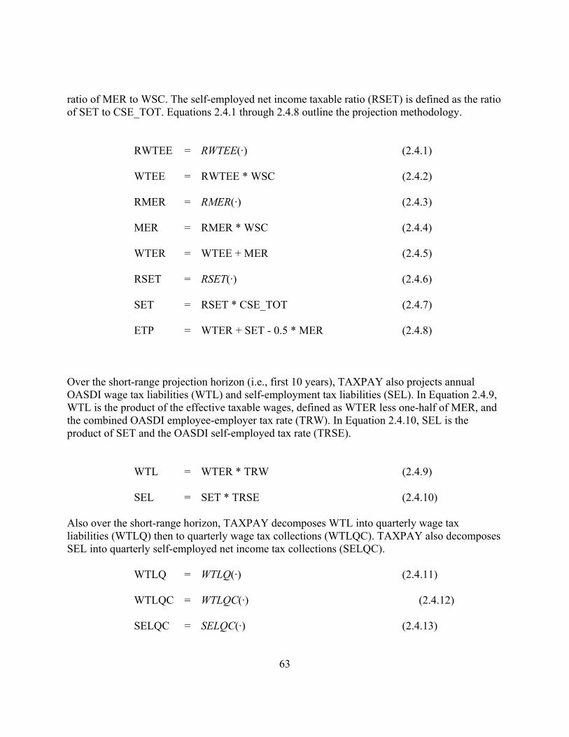
63

ratio of MER to WSC. The self-employed net income taxable ratio (RSET) is defined as the ratio of SET to CSE_TOT. Equations 2.4.1 through 2.4.8 outline the projection methodology.

RWTEE = RWTEE(·) (2.4.1)

WTEE = RWTEE * WSC (2.4.2)

RMER = RMER(·) (2.4.3)

MER = RMER * WSC (2.4.4)

WTER = WTEE + MER (2.4.5)

RSET = RSET(·) (2.4.6)

SET = RSET * CSE_TOT (2.4.7)

ETP = WTER + SET - 0.5 * MER (2.4.8) Over the short-range projection horizon (i.e., first 10 years), TAXPAY also projects annual OASDI wage tax liabilities (WTL) and self-employment tax liabilities (SEL). In Equation 2.4.9, WTL is the product of the effective taxable wages, defined as WTER less one-half of MER, and the combined OASDI employee-employer tax rate (TRW). In Equation 2.4.10, SEL is the product of SET and the OASDI self-employed tax rate (TRSE).

WTL = WTER * TRW (2.4.9)

SEL = SET * TRSE (2.4.10) Also over the short-range horizon, TAXPAY decomposes WTL into quarterly wage tax liabilities (WTLQ) then to quarterly wage tax collections (WTLQC). TAXPAY also decomposes SEL into quarterly self-employed net income tax collections (SELQC).

WTLQ = WTLQ(·) (2.4.11)

WTLQC = WTLQC(·) (2.4.12)

SELQC = SELQC(·) (2.4.13)

64

Finally, over the first two projected quarters, TAXPAY estimates of WTLQC and SELQC are replaced with ones from the most recent OMB FY Budget. And, over the first four projected quarters, TAXPAY includes estimates for appropriation adjustments (AA).

AA = AA(·) (2.4.14)

2.4.b. Input Data Long-Range OASDI Projection Data

Economics - Data from Sections 2.1, 2.2, and 2.3

Trustees Assumptions - (See Section 2.1.b.) Addfactors

Addfactors were included for RWTEE and RSET. The need for addfactors is reviewed each year and addfactors are implemented if necessary.

Other input data

• OASDI employee, employer, and self-employed tax rates from 1937 to the end of the long-range period. These contribution rates are set according to the Social Security Act of 1935 and amendments to the Act through 2004. The rates are updated when legislation mandates a change.

• Proportions of OASDI tax liabilities for self-employment earnings for the current and

prior calendar year estimated to be collected in each quarter through the end of the short-range period. (In any particular quarter, some self-employed individuals are paying taxes on earnings from the prior year and some are paying from the current year’s earnings.) Values are derived from historical data from the Office of Tax Analysis (OTA) in the Department of the Treasury for the amount of self-employment taxes transferred to the OASDI Trust Funds in each month split by the calendar year (either the current or the prior) in which the self-employment income was earned. The data are updated every year after historical information for a complete new year is received (usually in March).

• Payday adjustments are established by analysis of the calendar to determine the

number of likely paydays (particularly Fridays) in a quarter. Data for payday adjustments are available for calendar years covering the short-range period. Since the number of Fridays in future calendars are fixed, the payday adjustments do not require updating between trustee reports.

65

• FICA appropriation adjustments – Estimated amounts of OASI and DI appropriation

adjustments to include newly reported tax liability amounts including correction of past transfers of estimated amounts to the trust funds. Values are derived from historical data from the OTA for the amount of OASI and DI tax liability by quarter, SSA’s OS tabulations of taxable wages from IRS Forms 941, quarterly certification letter data from SSA’s OFPO, and our revenue model estimates of tax liabilities. Values are estimated for the four quarters of the trustees report year and for the following two quarters.

• Time trend adjustments to RWTEE for each calendar year of the short-range period.

Historical analysis suggests a “trend” rate of decline in RWTEE of about 0.0016 per year through 2001. This trend reflects a movement toward greater amounts of wages being paid to workers earning above the taxable maximum. We expect this trend to continue to the end of the short-range projection horizon, but at a slower rate. Consequently, we assume an adjustment factor of 0.4 such that the trend annual rate of decline from 2002 to the end of the short-range projection horizon is about 0.0006 per year (i.e., 0.0016 * 0.4). The time trend has not been updated since first decided upon. It will be changed if and when it is deemed appropriate.

• Data obtained from ORES by email for the amounts of single and multi-employer

refunds for the latest 5 years. Each year, data are updated.

• Data obtained from ORES are tabulations of quarterly Form 941 data. Data currently used are the OASDI, HI, and income taxable wages by sector for the most recent five years. The data represent changes in reported wages since the prior quarterly report. The most recent data are appended to previously reported data. Annual totals are computed and used to derive estimates of OASDI taxable wages by sector for the latest historical years.

• Data obtained from the most recently available 1.0% CWHS active file, maintained

on Social Security’s mainframe and made available by ORES. The years of data are 1951 to the third year prior to the current Trustees Report year. The data are used for comparison of OASDI taxable earnings from other sources.

• Data obtained from quarterly IRS Form 941 file, provided by OS. Data currently used

are the OASDI and HI taxable wages for 1978 to the most recent year available. The data represent changes in reported wages since the prior quarterly report. The most recent data are appended to previously reported data. Annual totals are computed and used to derive estimates of OASDI taxable wages for the most recent historical years.

• Data for the most recent ten years from the Quarterly EPOXY Report, received in

hard-copy and, more recently, electronic formats obtained from OS. The data

66

currently used are the total number of workers with OASDI taxable earnings, total number of workers with OASDI self-employed taxable earnings, distribution of number of HI workers by wage intervals, distribution of number of OASDI workers by wage intervals, number of persons with OASDI taxable wages, number of persons with HI taxable wages, number of persons with OASDI taxable self-employment, number of persons with HI taxable self-employment, number of workers with single-employer excess wages, and number of workers with multi-employer excess wages.

• Data obtained from the Quarterly Trust Fund Letter, received from OFPO. Data

currently used are OASDI and HI taxable wages accumulated from all Forms 941 and W-2 to date, and changes in self-employment earnings and self-reported tips since the prior Letter. These data are for for years 1978 to the most recent year available.

2.4.c. Development of Output Equation 2.4.1 - Employee Taxable Ratio (RWTEE)

Over the short-range projection horizon, the projected value for RWTEE is the sum of the model’s “raw” estimate and an “addfactor.” The raw estimate for RWTEE is dependent on the distribution of workers by wage interval, the RELMAX, RTP, the age-sex distribution of wage workers, and a time trend adjustment. The projected distribution of workers by wage interval is an average (or amalgam) distribution over the 1993 through 2004 period. Holding other factors constant, a distribution with relatively more workers with wages over the TAXMAX leads to a lower RWTEE. The RELMAX is defined as the ratio of the TAXMAX to the ACW. A higher RELMAX leads to a higher RWTEE. An increase in the RTP also leads to a higher RWTEE. The change in the projected RWTEE due to the change in the age-sex distribution of wage workers is calculated by allowing employment by age and sex to change while holding taxable ratios (and average covered wages) by age and sex constant to levels in 1996. The time trend adjustment reduces the level of RWTEE by about 0.6 percentage point over the short-range projection horizon.

The addfactor is the product of a “base” adjustment and an assumed weight. The base adjustment is defined as the actual value for RWTEE in the latest historical (or base) year less the raw estimated value for the same period. The weight has an assumed value of 0.9 for the first projected year, then values of 0.8 in the second projected year, 0.7 in the third projected year,…, and 0.0 in the tenth projected year (i.e., the end of the short-range projection horizon). The addfactor is necessary because we assume that the distribution of wage workers by earnings interval in the base year will gradually change to the amalgam distribution by the end of the short-range period and remain constant thereafter.

Over the long-range projection horizon, RWTEE is assumed to remain constant.

67

RWTEEs are also projected for various sub-aggregates including Federal Civilian employees under FERS and CSRS, Federal Civilian employees under CSRS only, S&L employees covered under OASDI, S&L employees covered under HI only, U.S. armed forces, and agriculture. The RWTEE for each sub-aggregate is dependent only on its sub-aggregate RELMAX, that is, the ratio of the TAXMAX to the sub-aggregate’s average covered wage.

Equation 2.4.3 - Multi-Employer Refund Wage Ratio (RMER)

The RMER is functionally related to the RWTEE. As RWTEE approaches one, then RMER approaches zero. In between the limit values, RMER is positive. Given the present position of RWTEE and RMER on the function, a projected decline in RWTEE leads to an increase in RMER.

The projected RMER is also dependent on RU. An increase in RU leads to a decrease in RMER.

Equation 2.4.6 - Self-Employed Net Income Taxable Ratio (RSET)

The RSET is disaggregated by type of self-employed worker, SEO and CMB_TOT.

SEO - The RSET is dependent on the distribution of self-employed workers by income interval and a RELMAX. The projected distribution of self-employed workers by income interval is set to the 1996 distribution. The RELMAX is defined here as the ratio of the TAXMAX to the average income for SEO. A higher RELMAX leads to a higher RSET.

CMB_TOT - Taxable self-employed net income for CMB_TOT is projected in two steps. First, a taxable earnings (wages and self-employed income) ratio for CMB_TOT is projected based on the 1996 distribution and a RELMAX defined as the ratio of the TAXMAX to the average covered earnings. The projected level of taxable earnings for CMB_TOT is the product of the estimated taxable earnings ratio for CMB_TOT and their covered earnings. Second, a taxable wage ratio for CMB_TOT is projected based on a RELMAX defined as the ratio of the TAXMAX to the average covered wage for CMB_TOT. The projected level of taxable wages for CMB_TOT is the product of the estimated taxable wage ratio for CMB_TOT and their covered wages.

Taxable self-employed net income for CMB_TOT is obtained by subtracting taxable wages from taxable earnings for CMB_TOT.

A “combined” RSET is calculated as the ratio of taxable self-employed net income for SEO and CMB_TOT to CSE_TOT. As with the RWTEE, the combined RSET is adjusted over the short-range period due to other factors (i.e., RTP, the age-sex distribution of workers, and a

68

trend). The effect of the other factors are taken from RWTEE and “scaled.” That is, RSET is adjusted by a percent effect (as opposed to percentage point) that is equal to the percent change in RWTEE due to changes in these other factors.

It is important to note that while the RWTEE is held constant after the short-range period, the RSETs for self-employed workers are not. After the short-range period, the projected RSETs for SEO and CMB_TOT continue to be dependent on their respective RELMAXs. Since by law the TAXMAX grows at the rate of the AWI and since ACSE is assumed to grow faster than the ACW (since only ACW declines with the growth in fringe benefits), the RELMAXs for self-employed workers decline over the long-range period while the RELMAX for wage workers is approximately constant. Hence, the RSETs for SEO and CMB_TOT are projected to decline over the long-range period while the RWTEE is held constant.

Equation 2.4.11 - Quarterly Wage Tax Liabilities (WTLQ)

The total WTLQ is summed from sector components that include the Federal Civilian, Federal Military, S&L, Private Household, Farm, Self-reported Tips, and residual Private Nonfarm. Sector WTLQ is determined by computing ratios of quarterly to annual liabilities for each quarter. For the Private Nonfarm, S&L, Federal Civilian and Military sectors, these “WTLQ ratios” are calculated for each quarter. Each is dependent on the quarterly distribution of WSD and the RWTEE for the relevant sector, and on a payday adjustment that takes into account the actual number of paydays that fall into a particular calendar quarter. WTLQ ratios are also calculated for each quarter for the other sectors. However, these are expected to be constants over the projection horizon.

Equation 2.4.12 - Quarterly Wage Tax Collections (WTLQC)

Employers incur tax liabilities when they pay wages to their employees. These liabilities are required to be deposited with the U.S. Treasury by employers based on the amount of total payroll tax liability (income taxes plus Social Security and Medicare taxes withheld) accumulated. Some very large employers must deposit their tax liabilities the next banking day after paying their employees. Other levels of accumulated tax liabilities require depositing within three days, by the middle of the following month, or by the end of the month following the quarter. If employers follow these deposit requirements, the result is that all tax liability for a particular quarter is deposited by the last day of the month following the end of the quarter. Thus, the WTLQC for any particular quarter are the sum of the tax liabilities deposited for wages paid in the same quarter and the liabilities deposited for wages paid in the prior quarter.

WTLQC is summed from sector components that include the Federal Civilian, Federal Military, Farm, S&L, and residual Private Nonfarm (including Private Household and Self-reported Tips). For the Federal Civilian and Military sectors, the WTLQC is set equal to its respective WTLQ since tax liabilities for the two sectors are collected immediately. The WTLQC for Farm is also set equal to its WTLQ, due in part to the fact that farms report tax

69

liabilities annually. For the S&L and Private Nonfarm sectors, WTLQC is the product of WTLQ and the proportion of WTLQ that should be deposited in the month following the end of each quarter. This proportion is based on the deposit requirements and estimates of accumulated tax liabilities, which in turn are based on firm size (or total wages paid).

Equation 2.4.13 - Quarterly Self-Employed Net Income Tax Collections (SELQC)

For wage workers, annual liabilities (WTL) are distributed to quarterly liabilities (WTLQ), which in turn are distributed to quarterly collections (WTLQC). However, for self-employed workers, annual liabilities (SEL) are distributed directly to SELQC, since the SSA only receives self-employed liability amounts on an annual basis (from tabulations of Form 1040 Schedule SE provided by IRS).

SEL for a particular calendar year is distributed as collections to the four quarters of that year and to the first three quarters of the next year. This distribution uses quarterly proportions that are based on an historical pattern of the amount of SEL collected in each month, as estimated by the OTA. The OTA estimates reflect IRS regulations that require self-employed workers to deposit estimated tax liabilities four times a year (January, April, June, and September).

Equation 2.4.14 - Appropriation Adjustments (AA)

70

We estimate WTLQC and SELQC for the next two quarters based on projected levels of WSD and Y in the various OMB FY Budgets. The Treasury uses these estimates to make initial appropriations to the OASDI Trust Funds over the period. Roughly one year after an initial appropriation has been made for a quarter, the initial appropriation is adjusted based on certified taxable wages reported on Forms 941 and W-2 and taxable self-employment income reported on Forms 1040 Schedule SE. This appropriation adjustment occurs quarterly and includes amounts due to newly-reported wages and self-employment income for all earlier periods.

FICA appropriation adjustments for wages are projected for all quarters for which we know what the Treasury will transfer. This generally means that we make estimates for adjustments to occur through the second quarter of the year following the Trustees Report year. The projected adjustment for each quarter is composed of two parts. The first estimates the error in the initial appropriation for the fourth earlier quarter. This error is defined as the difference between the Treasury’s initial appropriation and that portion of TAXPAY’s latest estimate for that quarter which is expected to be certified at the point when the adjustment is made. The second part is an estimate of the tax liability from additional certified wages for all previous periods and is based on an average of additional amounts over a recent historical period. These estimates are currently made in separate Excel files (generally named “EstimatedAppAdjAlt2.xls” and placed in a folder unique to the particular Trustees Report, e.g., \\wmpiet\usr\wmpiet\Excel\TR06), where they are further documented in a “Notes” sheet in the Excel file.

Appropriation adjustments for self-employment income are projected over the entire projection horizon based on the historical pattern of reporting. These estimates are made in the TAXPAY.

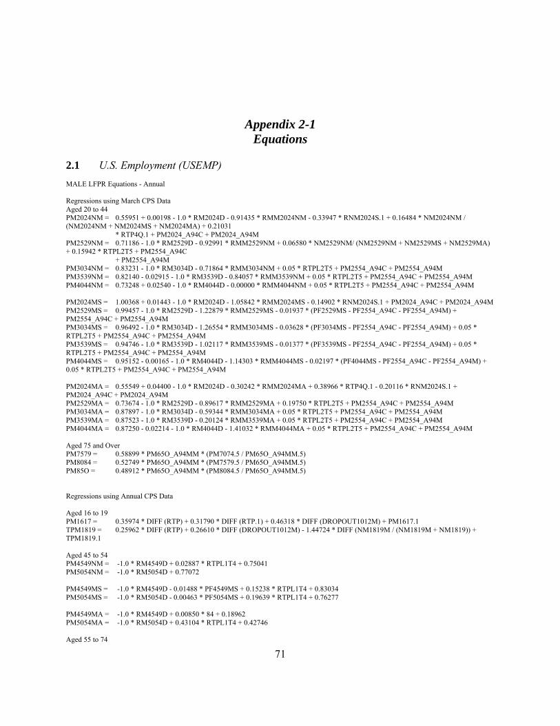
71

Appendix 2-1 Equations

2.1 U.S. Employment (USEMP) MALE LFPR Equations - Annual Regressions using March CPS Data Aged 20 to 44 PM2024NM = 0.55951 + 0.00198 - 1.0 * RM2024D - 0.91435 * RMM2024NM - 0.33947 * RNM2024S.1 + 0.16484 * NM2024NM / (NM2024NM + NM2024MS + NM2024MA) + 0.21031 * RTP4Q.1 + PM2024_A94C + PM2024_A94M PM2529NM = 0.71186 - 1.0 * RM2529D - 0.92991 * RMM2529NM + 0.06580 * NM2529NM/ (NM2529NM + NM2529MS + NM2529MA) + 0.15942 * RTPL2T5 + PM2554_A94C + PM2554_A94M PM3034NM = 0.83231 - 1.0 * RM3034D - 0.71864 * RMM3034NM + 0.05 * RTPL2T5 + PM2554_A94C + PM2554_A94M PM3539NM = 0.82140 - 0.02915 - 1.0 * RM3539D - 0.84057 * RMM3539NM + 0.05 * RTPL2T5 + PM2554_A94C + PM2554_A94M PM4044NM = 0.73248 + 0.02540 - 1.0 * RM4044D - 0.00000 * RMM4044NM + 0.05 * RTPL2T5 + PM2554_A94C + PM2554_A94M PM2024MS = 1.00368 + 0.01443 - 1.0 * RM2024D - 1.05842 * RMM2024MS - 0.14902 * RNM2024S.1 + PM2024_A94C + PM2024_A94M PM2529MS = 0.99457 - 1.0 * RM2529D - 1.22879 * RMM2529MS - 0.01937 * (PF2529MS - PF2554_A94C - PF2554_A94M) + PM2554_A94C + PM2554_A94M PM3034MS = 0.96492 - 1.0 * RM3034D - 1.26554 * RMM3034MS - 0.03628 * (PF3034MS - PF2554_A94C - PF2554_A94M) + 0.05 * RTPL2T5 + PM2554_A94C + PM2554_A94M PM3539MS = 0.94746 - 1.0 * RM3539D - 1.02117 * RMM3539MS - 0.01377 * (PF3539MS - PF2554_A94C - PF2554_A94M) + 0.05 * RTPL2T5 + PM2554_A94C + PM2554_A94M PM4044MS = 0.95152 - 0.00165 - 1.0 * RM4044D - 1.14303 * RMM4044MS - 0.02197 * (PF4044MS - PF2554_A94C - PF2554_A94M) + 0.05 * RTPL2T5 + PM2554_A94C + PM2554_A94M PM2024MA = 0.55549 + 0.04400 - 1.0 * RM2024D - 0.30242 * RMM2024MA + 0.38966 * RTP4Q.1 - 0.20116 * RNM2024S.1 + PM2024_A94C + PM2024_A94M PM2529MA = 0.73674 - 1.0 * RM2529D - 0.89617 * RMM2529MA + 0.19750 * RTPL2T5 + PM2554_A94C + PM2554_A94M PM3034MA = 0.87897 - 1.0 * RM3034D - 0.59344 * RMM3034MA + 0.05 * RTPL2T5 + PM2554_A94C + PM2554_A94M PM3539MA = 0.87523 - 1.0 * RM3539D - 0.20124 * RMM3539MA + 0.05 * RTPL2T5 + PM2554_A94C + PM2554_A94M PM4044MA = 0.87250 - 0.02214 - 1.0 * RM4044D - 1.41032 * RMM4044MA + 0.05 * RTPL2T5 + PM2554_A94C + PM2554_A94M Aged 75 and Over PM7579 = 0.58899 * PM65O_A94MM * (PM7074.5 / PM65O_A94MM.5) PM8084 = 0.52749 * PM65O_A94MM * (PM7579.5 / PM65O_A94MM.5) PM85O = 0.48912 * PM65O_A94MM * (PM8084.5 / PM65O_A94MM.5) Regressions using Annual CPS Data Aged 16 to 19 PM1617 = 0.35974 * DIFF (RTP) + 0.31790 * DIFF (RTP.1) + 0.46318 * DIFF (DROPOUT1012M) + PM1617.1 TPM1819 = 0.25962 * DIFF (RTP) + 0.26610 * DIFF (DROPOUT1012M) - 1.44724 * DIFF (NM1819M / (NM1819M + NM1819)) + TPM1819.1 Aged 45 to 54 PM4549NM = -1.0 * RM4549D + 0.02887 * RTPL1T4 + 0.75041 PM5054NM = -1.0 * RM5054D + 0.77072 PM4549MS = -1.0 * RM4549D - 0.01488 * PF4549MS + 0.15238 * RTPL1T4 + 0.83034 PM5054MS = -1.0 * RM5054D - 0.00463 * PF5054MS + 0.19639 * RTPL1T4 + 0.76277 PM4549MA = -1.0 * RM4549D + 0.00850 * 84 + 0.18962 PM5054MA = -1.0 * RM5054D + 0.43104 * RTPL1T4 + 0.42746 Aged 55 to 74

72

PM55 = 0.11202 * RTP.3 - 1.0 * RM55D + 0.01523 - 0.27650 + (0.24398 - 0.11202) -0.01 + (MOVAVG (3, PM5054_FE.2 + PM2554_94M_TE.2 + PM2554_90C_TE.2 + RM5054D.2) - 0.05338 * RTP.3 - 1)) PM56 = 0.10041 * RTP.3 - 1.0 * RM56D - 0.00180 + (PM55.1 + RM55D.1 - 0.11202 * RTP.4) PM57 = 0.13081 * RTP.3 - 1.0 * RM57D - 0.04182 + (PM56.1 + RM56D.1 - 0.10041 * RTP.4) PM58 = 0.24841 * RTP.3 - 1.0 * RM58D - 0.12905 + (PM57.1 + RM57D.1 - 0.13081 * RTP.4) PM59 = 0.25992 * RTP.3 - 1.0 * RM59D - 0.02818 + (PM58.1 + RM58D.1 - 0.24841 * RTP.4) PM60 = 0.31289 * RTP.3 - 1.0 * RM60D - 0.08886 + (PM59.1 + RM59D.1 - 0.25992 * RTP.4) PM61 = 0.32660 * RTP.3 - 1.0 * RM61D - 0.04412 + (PM60.1 + RM60D.1 - 0.31289 * RTP.4) PM62 = (1.0 - 1.0 * DIFF (RRADJ_M62) + 0.100 * DIFF (RETEST64U) + 0.15 * DIFF (RTP.2)) * (PM62.1 + RM62D.1) - RM62D PM63 = (1.0 - 1.0 * DIFF (RRADJ_M63) + 0.100 * DIFF (RETEST64U) + 0.15 * DIFF (RTP.2)) * (PM63.1 + RM63D.1) - RM63D PM64 = (1.0 - 1.0 * DIFF (RRADJ_M64) + 0.100 * DIFF (RETEST64U) + 0.15 * DIFF (RTP.2)) * (PM64.1 + RM64D.1) - RM64D PM65 = (1.0 - 1.0 * DIFF (RRADJ_M65) + 0.100 * DIFF (RETEST65) + 0.15 * DIFF (RTP.2)) * PM65.1 PM66 = (1.0 - 1.0 * DIFF (RRADJ_M66) + 0.100 * DIFF (RETEST66) + 0.15 * DIFF (RTP.2)) * PM66.1 PM67 = (1.0 - 1.0 * DIFF (RRADJ_M67) + 0.100 * DIFF (RETEST67) + 0.15 * DIFF (RTP.2)) * PM67.1 PM68 = (1.0 - 1.0 * DIFF (RRADJ_M68) + 0.100 * DIFF (RETEST68) + 0.15 * DIFF (RTP.2)) * PM68.1 PM69 = (1.0 - 1.0 * DIFF (RRADJ_M69) + 0.100 * DIFF (RETEST69) + 0.15 * DIFF (RTP.2)) * PM69.1 PM70 = (1.0 - 1.0 * DIFF (RRADJ_M70) + 0.15 * DIFF (RTP.2)) * PM70.1 PM71 = (0.04127 + 0.91152) * PM70.1 PM72 = (0.02632 + 0.90027) * PM71.1 PM73 = (0.05478 + 0.91456) * PM72.1 PM74 = (-0.02105 + 0.87355) * PM73.1 MALE LFPR Equations - Quarterly Regressions using March CPS Data Aged 20 to 44 PM2024NM = 0.55951 + 0.00198 - 1.0 * RM2024D - 0.91435 * RMM2024NM - 0.33947 * RNM2024S +0.16484 * NM2024NM / (NM2024NM + NM2024MS + NM2024MA) +0.21031 * RTP.1 + PM2024_A94C + PM2024_A94M PM2529NM = 0.71186 - 1.0 * RM2529D - 0.92991 * RMM2529NM +0.06580 * NM2529NM / (NM2529NM + NM2529MS + NM2529MA) +0.15942 * MOVAVG (4, RTP.2) + PM2554_A94C + PM2554_A94M PM3034NM = 0.83231 - 1.0 * RM3034D - 0.71864 * RMM3034NM + 0.05 * MOVAVG (4, RTP.2) + PM2554_A94C + PM2554_A94M PM3539NM = 0.82140 - 0.02915 - 1.0 * RM3539D - 0.84057 * RMM3539NM + 0.05 * MOVAVG (4, RTP.2) + PM2554_A94C + PM2554_A94M PM4044NM = 0.73248 + 0.02540 - 1.0 * RM4044D - 0.00000 * RMM4044NM + 0.05 * MOVAVG (4, RTP.2) + PM2554_A94C + PM2554_A94M PM2024MS = 1.00368 + 0.01443 - 1.0 * RM2024D - 1.05842 * RMM2024MS - 0.14902 * RNM2024S + PM2024_A94C + PM2024_A94M PM2529MS = 0.99457 - 1.0 * RM2529D - 1.22879 * RMM2529MS - 0.01937 * MOVAVG (4, (PF2529MS.1 - PF2554_A94C.1 - PF2554_A94M.1)) + PM2554_A94C + PM2554_A94M PM3034MS = 0.96492 - 1.0 * RM3034D - 1.26554 * RMM3034MS - 0.03628 * MOVAVG (4, (PF3034MS.1 - PF2554_A94C.1 - PF2554_A94M.1)) + 0.05 * MOVAVG (4, RTP.2) + PM2554_A94C + PM2554_A94M PM3539MS = 0.94746 - 1.0 * RM3539D - 1.02117 * RMM3539MS - 0.01377 * MOVAVG (4, (PF3539MS.1 - PF2554_A94C.1 - PF2554_A94M.1)) + 0.05 * MOVAVG (4, RTP.2) + PM2554_A94C + PM2554_A94M PM4044MS = 0.95152 - 0.00139 - 1.0 * RM4044D - 1.14303 * RMM4044MS - 0.02197 * MOVAVG (4, (PF4044MS.1 - PF2554_A94C.1 - PF2554_A94M.1)) + 0.05 * MOVAVG (4, RTP.2) + PM2554_A94C + PM2554_A94M PM2024MA = 0.55549 + 0.04400 - 1.0 * RM2024D - 0.30242 * RMM2024MA +0.38966 * RTP.1 - 0.20116 * RNM2024S + PM2024_A94C + PM2024_A94M PM2529MA = 0.73674 - 1.0 * RM2529D - 0.89617 * RMM2529MA +0.19750 * MOVAVG (4, RTP.2) + PM2554_A94C + PM2554_A94M PM3034MA = 0.87897 - 1.0 * RM3034D - 0.59344 * RMM3034MA + 0.05 * MOVAVG (4, RTP.2) + PM2554_A94C + PM2554_A94M PM3539MA = 0.87523 - 1.0 * RM3539D - 0.20124 * RMM3539MA + 0.05 * MOVAVG (4, RTP.2) + PM2554_A94C + PM2554_A94M PM4044MA = 0.87250 - 0.02214 - 1.0 * RM4044D - 1.41032 * RMM4044MA + 0.05 * MOVAVG (4, RTP.2) + PM2554_A94C + PM2554_A94M Aged 75 and Over PM7579 = 0.58899 * PM65O_A94MM * MOVAVG (4, PM7074.20)

73

PM8084 = 0.52749 * PM65O_A94MM * MOVAVG (4, PM7579.20) PM85O = 0.48912 * PM65O_A94MM * MOVAVG (4, PM8084.20) Regressions using Annual CPS Data Aged 16 to 19 PM1617 = 0.35974 * DIFF (RTP.1) + 0.31790 * DIFF (RTP.5) + 0.46318 * DIFF (DROPOUT1012M) + PM1617.1 TPM1819 = 0.25962 * DIFF (RTP.1) + 0.26610 * DIFF (DROPOUT1012M) - 1.44724 * DIFF (RM1819M) + TPM1819.1 Aged 45 to 54 PM4549NM = -1.0 * RM4549D + 0.02887 * MOVAVG (4, RTP.1) + 0.75041 PM5054NM = -1.0 * RM5054D + 0.77072 PM4549MS = -1.0 * RM4549D - 0.01488 * PF4549MS + 0.15238 * MOVAVG (4, RTP.1) + 0.83034 PM5054MS = -1.0 * RM5054D - 0.00463 * PF5054MS + 0.19639 * MOVAVG (4, RTP.1) + 0.76277 PM4549MA = -1.0 * RM4549D + 0.00850 * 84 + 0.18962 PM5054MA = -1.0 * RM5054D + 0.43104 * MOVAVG (4, RTP.1) + 0.42746 Aged 55 to 74 PM55 = 0.11202 * MOVAVG (5, RTP.10) - 1.0 * RM55D + 0.01523 -0.27650 + (0.24398 -0.11202) -0.01 + (PM5054L_FE) PM56 = 0.10041 * MOVAVG (5, RTP.10) - 1.0 * RM56D - 0.00180 + (PM55.4 + RM55D.4 - 0.11202 * MOVAVG (5, RTP.14)) PM57 = 0.13081 * MOVAVG (5, RTP.10) - 1.0 * RM57D - 0.04182 + (PM56.4 + RM56D.4 - 0.10041 * MOVAVG (5, RTP.14)) PM58 = 0.24841 * MOVAVG (5, RTP.10) - 1.0 * RM58D - 0.12905 + (PM57.4 + RM57D.4 - 0.13081 * MOVAVG (5, RTP.14)) PM59 = 0.25992 * MOVAVG (5, RTP.10) - 1.0 * RM59D - 0.02818 + (PM58.4 + RM58D.4 - 0.24841 * MOVAVG (5, RTP.14)) PM60 = 0.31289 * MOVAVG (5, RTP.10) - 1.0 * RM60D - 0.08886 + (PM59.4 + RM59D.4 - 0.25992 * MOVAVG (5, RTP.14)) PM61 = 0.32660 * MOVAVG (5, RTP.10) - 1.0 * RM61D - 0.04412 + (PM60.4 + RM60D.4 - 0.31289 * MOVAVG (5, RTP.14)) PM62 = (1.0 - 1.0 * DIFF (RRADJ_M62) + 0.100 * DIFF (RETEST64U) + 0.15 * DIFF (MOVAVG (5, RTP.6))) * (PM62.1 + RM62D.1) - RM62D PM63 = (1.0 - 1.0 * DIFF (RRADJ_M63) + 0.100 * DIFF (RETEST64U) + 0.15 * DIFF (MOVAVG (5, RTP.6))) * (PM63.1 + RM63D.1) - RM63D PM64 = (1.0 - 1.0 * DIFF (RRADJ_M64) + 0.100 * DIFF (RETEST64U) + 0.15 * DIFF (MOVAVG (5, RTP.6))) * (PM64.1 + RM64D.1) - RM64D PM65 = (1.0 - 1.0 * DIFF (RRADJ_M65) + 0.100 * DIFF (RETEST65) + 0.15 * DIFF (MOVAVG (5, RTP.6))) * PM65.1 PM66 = (1.0 - 1.0 * DIFF (RRADJ_M66) + 0.100 * DIFF (RETEST66) + 0.15 * DIFF (MOVAVG (5, RTP.6))) * PM66.1 PM67 = (1.0 - 1.0 * DIFF (RRADJ_M67) + 0.100 * DIFF (RETEST67) + 0.15 * DIFF (MOVAVG (5, RTP.6))) * PM67.1 PM68 = (1.0 - 1.0 * DIFF (RRADJ_M68) + 0.100 * DIFF (RETEST68) + 0.15 * DIFF (MOVAVG (5, RTP.6))) * PM68.1 PM69 = (1.0 - 1.0 * DIFF (RRADJ_M69) + 0.100 * DIFF (RETEST69) + 0.15 * DIFF (MOVAVG (5, RTP.6))) * PM69.1 PM70 = (1.0 - 1.0 * DIFF (RRADJ_M70) + 0.15 * DIFF (MOVAVG (5, RTP.6))) * PM70.1 PM71 = (0.04127 + 0.91152) * PM70.4 PM72 = (0.02632 + 0.90027) * PM71.4 PM73 = (0.05478 + 0.91456) * PM72.4 PM74 = (-0.02105 + 0.87355) * PM73.4 Aggregation of Equations from Regressions using March CPS Data Using Quarterly Seasonal Adjustment Weights Aged 20 to 44 TPM2024 = ((PM2024NM * RM2024NM + PM2024MS * RM2024MS + PM2024MA * RM2024MA) + 0.006) * 1.021 TPM2529 = ((PM2529NM * RM2529NM + PM2529MS * RM2529MS + PM2529MA * RM2529MA) + 0.005) * 0.997 TPM3034 = ((PM3034NM * RM3034NM + PM3034MS * RM3034MS + PM3034MA * RM3034MA) + 0.005) * 0.997 TPM3539 = ((PM3539NM * RM3539NM + PM3539MS * RM3539MS + PM3539MA * RM3539MA) + 0.010) * 0.999 TPM4044 = ((PM4044NM * RM4044NM + PM4044MS * RM4044MS + PM4044MA * RM4044MA) + 0.010) * 0.999 PM4549 = ((PM4549NM * RM4549NM + PM4549MS * RM4549MS + PM4549MA * RM4549MA) + 0.003) * 0.999 PM5054 = ((PM5054NM * RM5054NM + PM5054MS * RM5054MS + PM5054MA * RM5054MA) + 0.003) * 0.999 Aged 75 and Over PM75O = ((PM7579 * NM7579/NM75O+ PM8084 * NM8084/NM75O+ PM85O* NM85O/NM75O) + 0.000) * 1.000 Aggregation of Equations from Regressions using Annual CPS Data Aged 55 to 74

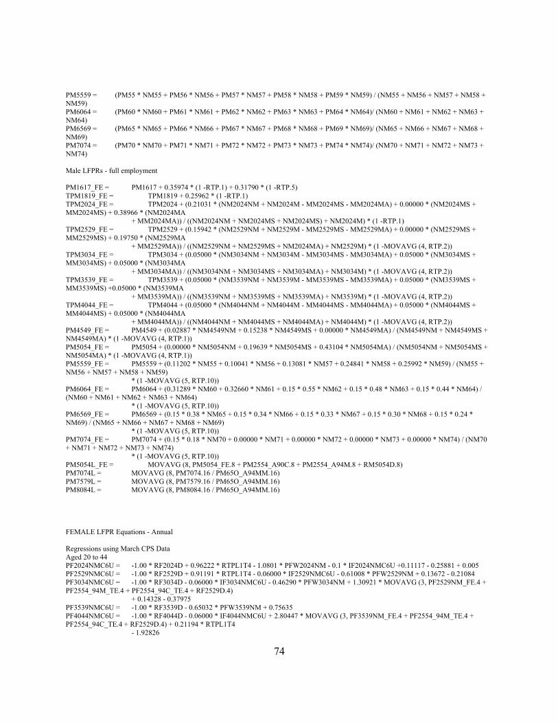
74

PM5559 = (PM55 * NM55 + PM56 * NM56 + PM57 * NM57 + PM58 * NM58 + PM59 * NM59) / (NM55 + NM56 + NM57 + NM58 + NM59) PM6064 = (PM60 * NM60 + PM61 * NM61 + PM62 * NM62 + PM63 * NM63 + PM64 * NM64)/ (NM60 + NM61 + NM62 + NM63 + NM64) PM6569 = (PM65 * NM65 + PM66 * NM66 + PM67 * NM67 + PM68 * NM68 + PM69 * NM69)/ (NM65 + NM66 + NM67 + NM68 + NM69) PM7074 = (PM70 * NM70 + PM71 * NM71 + PM72 * NM72 + PM73 * NM73 + PM74 * NM74)/ (NM70 + NM71 + NM72 + NM73 + NM74) Male LFPRs - full employment PM1617_FE = PM1617 + 0.35974 * (1 -RTP.1) + 0.31790 * (1 -RTP.5) TPM1819_FE = TPM1819 + 0.25962 * (1 -RTP.1) TPM2024_FE = TPM2024 + (0.21031 * (NM2024NM + NM2024M - MM2024MS - MM2024MA) + 0.00000 * (NM2024MS + MM2024MS) + 0.38966 * (NM2024MA + MM2024MA)) / ((NM2024NM + NM2024MS + NM2024MS) + NM2024M) * (1 -RTP.1) TPM2529_FE = TPM2529 + (0.15942 * (NM2529NM + NM2529M - MM2529MS - MM2529MA) + 0.00000 * (NM2529MS + MM2529MS) + 0.19750 * (NM2529MA + MM2529MA)) / ((NM2529NM + NM2529MS + NM2024MA) + NM2529M) * (1 -MOVAVG (4, RTP.2)) TPM3034_FE = TPM3034 + (0.05000 * (NM3034NM + NM3034M - MM3034MS - MM3034MA) + 0.05000 * (NM3034MS + MM3034MS) + 0.05000 * (NM3034MA + MM3034MA)) / ((NM3034NM + NM3034MS + NM3034MA) + NM3034M) * (1 -MOVAVG (4, RTP.2)) TPM3539_FE = TPM3539 + (0.05000 * (NM3539NM + NM3539M - MM3539MS - MM3539MA) + 0.05000 * (NM3539MS + MM3539MS) +0.05000 * (NM3539MA + MM3539MA)) / ((NM3539NM + NM3539MS + NM3539MA) + NM3539M) * (1 -MOVAVG (4, RTP.2)) TPM4044_FE = TPM4044 + (0.05000 * (NM4044NM + NM4044M - MM4044MS - MM4044MA) + 0.05000 * (NM4044MS + MM4044MS) + 0.05000 * (NM4044MA + MM4044MA)) / ((NM4044NM + NM4044MS + NM4044MA) + NM4044M) * (1 -MOVAVG (4, RTP.2)) PM4549_FE = PM4549 + (0.02887 * NM4549NM + 0.15238 * NM4549MS + 0.00000 * NM4549MA) / (NM4549NM + NM4549MS + NM4549MA) * (1 -MOVAVG (4, RTP.1)) PM5054_FE = PM5054 + (0.00000 * NM5054NM + 0.19639 * NM5054MS + 0.43104 * NM5054MA) / (NM5054NM + NM5054MS + NM5054MA) * (1 -MOVAVG (4, RTP.1)) PM5559_FE = PM5559 + (0.11202 * NM55 + 0.10041 * NM56 + 0.13081 * NM57 + 0.24841 * NM58 + 0.25992 * NM59) / (NM55 + NM56 + NM57 + NM58 + NM59) * (1 -MOVAVG (5, RTP.10)) PM6064_FE = PM6064 + (0.31289 * NM60 + 0.32660 * NM61 + 0.15 * 0.55 * NM62 + 0.15 * 0.48 * NM63 + 0.15 * 0.44 * NM64) / (NM60 + NM61 + NM62 + NM63 + NM64) * (1 -MOVAVG (5, RTP.10)) PM6569_FE = PM6569 + (0.15 * 0.38 * NM65 + 0.15 * 0.34 * NM66 + 0.15 * 0.33 * NM67 + 0.15 * 0.30 * NM68 + 0.15 * 0.24 * NM69) / (NM65 + NM66 + NM67 + NM68 + NM69) * (1 -MOVAVG (5, RTP.10)) PM7074_FE = PM7074 + (0.15 * 0.18 * NM70 + 0.00000 * NM71 + 0.00000 * NM72 + 0.00000 * NM73 + 0.00000 * NM74) / (NM70 + NM71 + NM72 + NM73 + NM74) * (1 -MOVAVG (5, RTP.10)) PM5054L_FE = MOVAVG (8, PM5054_FE.8 + PM2554_A90C.8 + PM2554_A94M.8 + RM5054D.8) PM7074L = MOVAVG (8, PM7074.16 / PM65O_A94MM.16) PM7579L = MOVAVG (8, PM7579.16 / PM65O_A94MM.16) PM8084L = MOVAVG (8, PM8084.16 / PM65O_A94MM.16) FEMALE LFPR Equations - Annual Regressions using March CPS Data Aged 20 to 44 PF2024NMC6U = -1.00 * RF2024D + 0.96222 * RTPL1T4 - 1.0801 * PFW2024NM - 0.1 * IF2024NMC6U +0.11117 - 0.25881 + 0.005 PF2529NMC6U = -1.00 * RF2529D + 0.91191 * RTPL1T4 - 0.06000 * IF2529NMC6U - 0.61008 * PFW2529NM + 0.13672 - 0.21084 PF3034NMC6U = -1.00 * RF3034D - 0.06000 * IF3034NMC6U - 0.46290 * PFW3034NM + 1.30921 * MOVAVG (3, PF2529NM_FE.4 + PF2554_94M_TE.4 + PF2554_94C_TE.4 + RF2529D.4) + 0.14328 - 0.37975 PF3539NMC6U = -1.00 * RF3539D - 0.65032 * PFW3539NM + 0.75635 PF4044NMC6U = -1.00 * RF4044D - 0.06000 * IF4044NMC6U + 2.80447 * MOVAVG (3, PF3539NM_FE.4 + PF2554_94M_TE.4 + PF2554_94C_TE.4 + RF2529D.4) + 0.21194 * RTPL1T4 - 1.92826

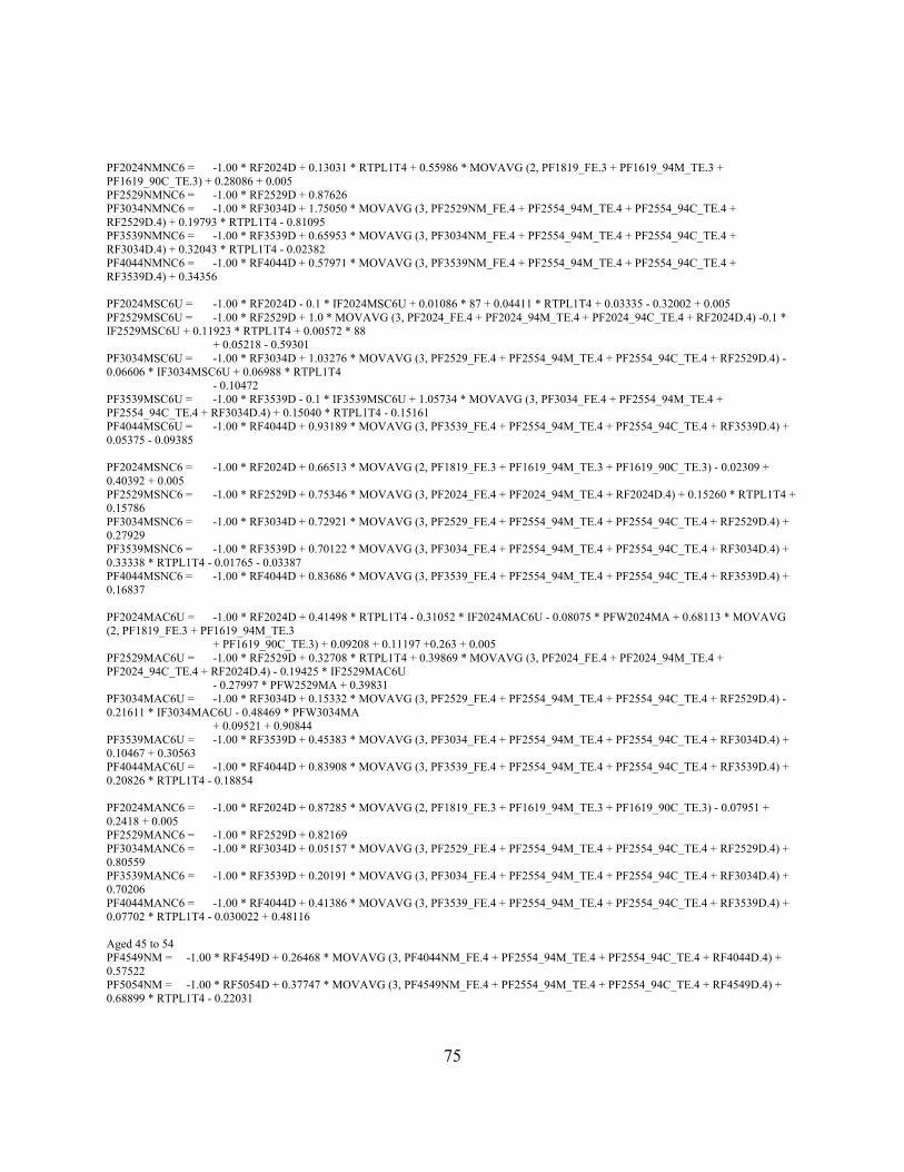
75

PF2024NMNC6 = -1.00 * RF2024D + 0.13031 * RTPL1T4 + 0.55986 * MOVAVG (2, PF1819_FE.3 + PF1619_94M_TE.3 + PF1619_90C_TE.3) + 0.28086 + 0.005 PF2529NMNC6 = -1.00 * RF2529D + 0.87626 PF3034NMNC6 = -1.00 * RF3034D + 1.75050 * MOVAVG (3, PF2529NM_FE.4 + PF2554_94M_TE.4 + PF2554_94C_TE.4 + RF2529D.4) + 0.19793 * RTPL1T4 - 0.81095 PF3539NMNC6 = -1.00 * RF3539D + 0.65953 * MOVAVG (3, PF3034NM_FE.4 + PF2554_94M_TE.4 + PF2554_94C_TE.4 + RF3034D.4) + 0.32043 * RTPL1T4 - 0.02382 PF4044NMNC6 = -1.00 * RF4044D + 0.57971 * MOVAVG (3, PF3539NM_FE.4 + PF2554_94M_TE.4 + PF2554_94C_TE.4 + RF3539D.4) + 0.34356 PF2024MSC6U = -1.00 * RF2024D - 0.1 * IF2024MSC6U + 0.01086 * 87 + 0.04411 * RTPL1T4 + 0.03335 - 0.32002 + 0.005 PF2529MSC6U = -1.00 * RF2529D + 1.0 * MOVAVG (3, PF2024_FE.4 + PF2024_94M_TE.4 + PF2024_94C_TE.4 + RF2024D.4) -0.1 * IF2529MSC6U + 0.11923 * RTPL1T4 + 0.00572 * 88 + 0.05218 - 0.59301 PF3034MSC6U = -1.00 * RF3034D + 1.03276 * MOVAVG (3, PF2529_FE.4 + PF2554_94M_TE.4 + PF2554_94C_TE.4 + RF2529D.4) - 0.06606 * IF3034MSC6U + 0.06988 * RTPL1T4 - 0.10472 PF3539MSC6U = -1.00 * RF3539D - 0.1 * IF3539MSC6U + 1.05734 * MOVAVG (3, PF3034_FE.4 + PF2554_94M_TE.4 + PF2554_94C_TE.4 + RF3034D.4) + 0.15040 * RTPL1T4 - 0.15161 PF4044MSC6U = -1.00 * RF4044D + 0.93189 * MOVAVG (3, PF3539_FE.4 + PF2554_94M_TE.4 + PF2554_94C_TE.4 + RF3539D.4) + 0.05375 - 0.09385 PF2024MSNC6 = -1.00 * RF2024D + 0.66513 * MOVAVG (2, PF1819_FE.3 + PF1619_94M_TE.3 + PF1619_90C_TE.3) - 0.02309 + 0.40392 + 0.005 PF2529MSNC6 = -1.00 * RF2529D + 0.75346 * MOVAVG (3, PF2024_FE.4 + PF2024_94M_TE.4 + RF2024D.4) + 0.15260 * RTPL1T4 + 0.15786 PF3034MSNC6 = -1.00 * RF3034D + 0.72921 * MOVAVG (3, PF2529_FE.4 + PF2554_94M_TE.4 + PF2554_94C_TE.4 + RF2529D.4) + 0.27929 PF3539MSNC6 = -1.00 * RF3539D + 0.70122 * MOVAVG (3, PF3034_FE.4 + PF2554_94M_TE.4 + PF2554_94C_TE.4 + RF3034D.4) + 0.33338 * RTPL1T4 - 0.01765 - 0.03387 PF4044MSNC6 = -1.00 * RF4044D + 0.83686 * MOVAVG (3, PF3539_FE.4 + PF2554_94M_TE.4 + PF2554_94C_TE.4 + RF3539D.4) + 0.16837 PF2024MAC6U = -1.00 * RF2024D + 0.41498 * RTPL1T4 - 0.31052 * IF2024MAC6U - 0.08075 * PFW2024MA + 0.68113 * MOVAVG (2, PF1819_FE.3 + PF1619_94M_TE.3 + PF1619_90C_TE.3) + 0.09208 + 0.11197 +0.263 + 0.005 PF2529MAC6U = -1.00 * RF2529D + 0.32708 * RTPL1T4 + 0.39869 * MOVAVG (3, PF2024_FE.4 + PF2024_94M_TE.4 + PF2024_94C_TE.4 + RF2024D.4) - 0.19425 * IF2529MAC6U - 0.27997 * PFW2529MA + 0.39831 PF3034MAC6U = -1.00 * RF3034D + 0.15332 * MOVAVG (3, PF2529_FE.4 + PF2554_94M_TE.4 + PF2554_94C_TE.4 + RF2529D.4) - 0.21611 * IF3034MAC6U - 0.48469 * PFW3034MA + 0.09521 + 0.90844 PF3539MAC6U = -1.00 * RF3539D + 0.45383 * MOVAVG (3, PF3034_FE.4 + PF2554_94M_TE.4 + PF2554_94C_TE.4 + RF3034D.4) + 0.10467 + 0.30563 PF4044MAC6U = -1.00 * RF4044D + 0.83908 * MOVAVG (3, PF3539_FE.4 + PF2554_94M_TE.4 + PF2554_94C_TE.4 + RF3539D.4) + 0.20826 * RTPL1T4 - 0.18854 PF2024MANC6 = -1.00 * RF2024D + 0.87285 * MOVAVG (2, PF1819_FE.3 + PF1619_94M_TE.3 + PF1619_90C_TE.3) - 0.07951 + 0.2418 + 0.005 PF2529MANC6 = -1.00 * RF2529D + 0.82169 PF3034MANC6 = -1.00 * RF3034D + 0.05157 * MOVAVG (3, PF2529_FE.4 + PF2554_94M_TE.4 + PF2554_94C_TE.4 + RF2529D.4) + 0.80559 PF3539MANC6 = -1.00 * RF3539D + 0.20191 * MOVAVG (3, PF3034_FE.4 + PF2554_94M_TE.4 + PF2554_94C_TE.4 + RF3034D.4) + 0.70206 PF4044MANC6 = -1.00 * RF4044D + 0.41386 * MOVAVG (3, PF3539_FE.4 + PF2554_94M_TE.4 + PF2554_94C_TE.4 + RF3539D.4) + 0.07702 * RTPL1T4 - 0.030022 + 0.48116 Aged 45 to 54 PF4549NM = -1.00 * RF4549D + 0.26468 * MOVAVG (3, PF4044NM_FE.4 + PF2554_94M_TE.4 + PF2554_94C_TE.4 + RF4044D.4) + 0.57522 PF5054NM = -1.00 * RF5054D + 0.37747 * MOVAVG (3, PF4549NM_FE.4 + PF2554_94M_TE.4 + PF2554_94C_TE.4 + RF4549D.4) + 0.68899 * RTPL1T4 - 0.22031

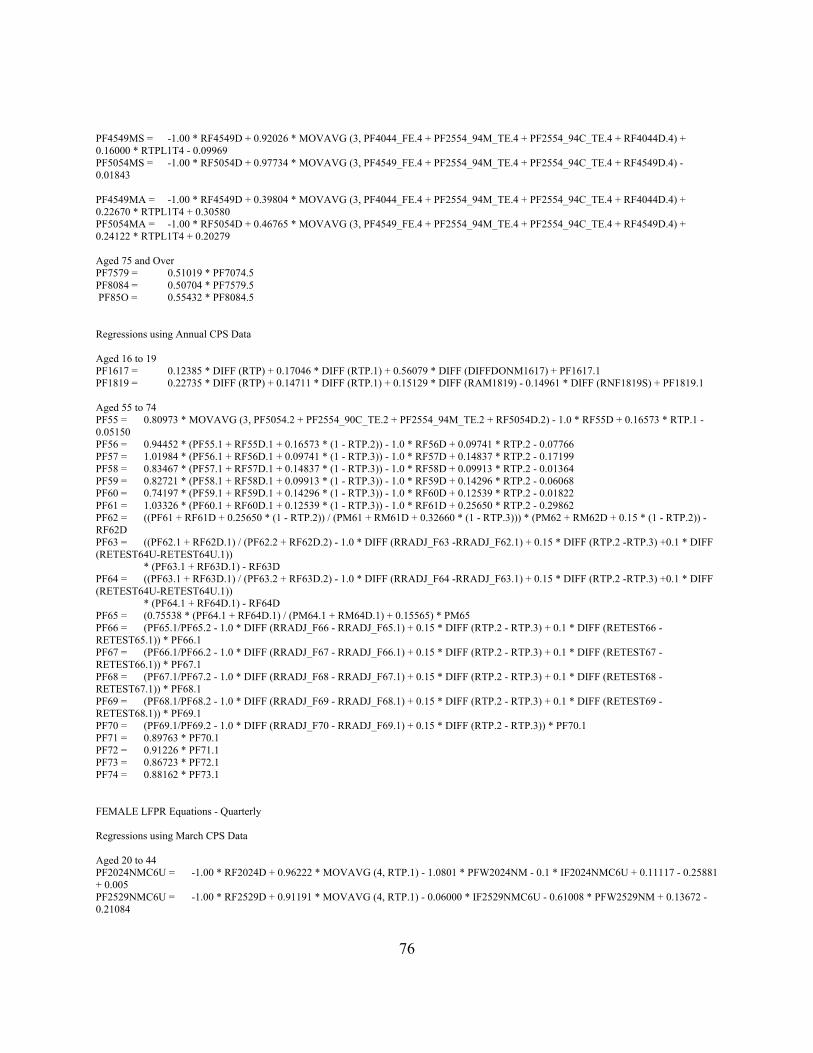
76

PF4549MS = -1.00 * RF4549D + 0.92026 * MOVAVG (3, PF4044_FE.4 + PF2554_94M_TE.4 + PF2554_94C_TE.4 + RF4044D.4) + 0.16000 * RTPL1T4 - 0.09969 PF5054MS = -1.00 * RF5054D + 0.97734 * MOVAVG (3, PF4549_FE.4 + PF2554_94M_TE.4 + PF2554_94C_TE.4 + RF4549D.4) - 0.01843 PF4549MA = -1.00 * RF4549D + 0.39804 * MOVAVG (3, PF4044_FE.4 + PF2554_94M_TE.4 + PF2554_94C_TE.4 + RF4044D.4) + 0.22670 * RTPL1T4 + 0.30580 PF5054MA = -1.00 * RF5054D + 0.46765 * MOVAVG (3, PF4549_FE.4 + PF2554_94M_TE.4 + PF2554_94C_TE.4 + RF4549D.4) + 0.24122 * RTPL1T4 + 0.20279 Aged 75 and Over PF7579 = 0.51019 * PF7074.5 PF8084 = 0.50704 * PF7579.5 PF85O = 0.55432 * PF8084.5 Regressions using Annual CPS Data Aged 16 to 19 PF1617 = 0.12385 * DIFF (RTP) + 0.17046 * DIFF (RTP.1) + 0.56079 * DIFF (DIFFDONM1617) + PF1617.1 PF1819 = 0.22735 * DIFF (RTP) + 0.14711 * DIFF (RTP.1) + 0.15129 * DIFF (RAM1819) - 0.14961 * DIFF (RNF1819S) + PF1819.1 Aged 55 to 74 PF55 = 0.80973 * MOVAVG (3, PF5054.2 + PF2554_90C_TE.2 + PF2554_94M_TE.2 + RF5054D.2) - 1.0 * RF55D + 0.16573 * RTP.1 - 0.05150 PF56 = 0.94452 * (PF55.1 + RF55D.1 + 0.16573 * (1 - RTP.2)) - 1.0 * RF56D + 0.09741 * RTP.2 - 0.07766 PF57 = 1.01984 * (PF56.1 + RF56D.1 + 0.09741 * (1 - RTP.3)) - 1.0 * RF57D + 0.14837 * RTP.2 - 0.17199 PF58 = 0.83467 * (PF57.1 + RF57D.1 + 0.14837 * (1 - RTP.3)) - 1.0 * RF58D + 0.09913 * RTP.2 - 0.01364 PF59 = 0.82721 * (PF58.1 + RF58D.1 + 0.09913 * (1 - RTP.3)) - 1.0 * RF59D + 0.14296 * RTP.2 - 0.06068 PF60 = 0.74197 * (PF59.1 + RF59D.1 + 0.14296 * (1 - RTP.3)) - 1.0 * RF60D + 0.12539 * RTP.2 - 0.01822 PF61 = 1.03326 * (PF60.1 + RF60D.1 + 0.12539 * (1 - RTP.3)) - 1.0 * RF61D + 0.25650 * RTP.2 - 0.29862 PF62 = ((PF61 + RF61D + 0.25650 * (1 - RTP.2)) / (PM61 + RM61D + 0.32660 * (1 - RTP.3))) * (PM62 + RM62D + 0.15 * (1 - RTP.2)) - RF62D PF63 = ((PF62.1 + RF62D.1) / (PF62.2 + RF62D.2) - 1.0 * DIFF (RRADJ_F63 -RRADJ_F62.1) + 0.15 * DIFF (RTP.2 -RTP.3) +0.1 * DIFF (RETEST64U-RETEST64U.1)) * (PF63.1 + RF63D.1) - RF63D PF64 = ((PF63.1 + RF63D.1) / (PF63.2 + RF63D.2) - 1.0 * DIFF (RRADJ_F64 -RRADJ_F63.1) + 0.15 * DIFF (RTP.2 -RTP.3) +0.1 * DIFF (RETEST64U-RETEST64U.1)) * (PF64.1 + RF64D.1) - RF64D PF65 = (0.75538 * (PF64.1 + RF64D.1) / (PM64.1 + RM64D.1) + 0.15565) * PM65 PF66 = (PF65.1/PF65.2 - 1.0 * DIFF (RRADJ_F66 - RRADJ_F65.1) + 0.15 * DIFF (RTP.2 - RTP.3) + 0.1 * DIFF (RETEST66 - RETEST65.1)) * PF66.1 PF67 = (PF66.1/PF66.2 - 1.0 * DIFF (RRADJ_F67 - RRADJ_F66.1) + 0.15 * DIFF (RTP.2 - RTP.3) + 0.1 * DIFF (RETEST67 - RETEST66.1)) * PF67.1 PF68 = (PF67.1/PF67.2 - 1.0 * DIFF (RRADJ_F68 - RRADJ_F67.1) + 0.15 * DIFF (RTP.2 - RTP.3) + 0.1 * DIFF (RETEST68 - RETEST67.1)) * PF68.1 PF69 = (PF68.1/PF68.2 - 1.0 * DIFF (RRADJ_F69 - RRADJ_F68.1) + 0.15 * DIFF (RTP.2 - RTP.3) + 0.1 * DIFF (RETEST69 - RETEST68.1)) * PF69.1 PF70 = (PF69.1/PF69.2 - 1.0 * DIFF (RRADJ_F70 - RRADJ_F69.1) + 0.15 * DIFF (RTP.2 - RTP.3)) * PF70.1 PF71 = 0.89763 * PF70.1 PF72 = 0.91226 * PF71.1 PF73 = 0.86723 * PF72.1 PF74 = 0.88162 * PF73.1 FEMALE LFPR Equations - Quarterly Regressions using March CPS Data Aged 20 to 44 PF2024NMC6U = -1.00 * RF2024D + 0.96222 * MOVAVG (4, RTP.1) - 1.0801 * PFW2024NM - 0.1 * IF2024NMC6U + 0.11117 - 0.25881 + 0.005 PF2529NMC6U = -1.00 * RF2529D + 0.91191 * MOVAVG (4, RTP.1) - 0.06000 * IF2529NMC6U - 0.61008 * PFW2529NM + 0.13672 - 0.21084

77

PF3034NMC6U = -1.00 * RF3034D - 0.06000 * IF3034NMC6U - 0.46290 * PFW3034NM + 1.30921 * PF2529NML_FE + 0.14328 - 0.37975 PF3539NMC6U = -1.00 * RF3539D - 0.65032 * PFW3539NM + 0.75635 PF4044NMC6U = -1.00 * RF4044D - 0.06000 * IF4044NMC6U + 2.80447 * PF3539NML_FE + 0.21194 * MOVAVG (4, RTP.1) - 1.92826 PF2024NMNC6 = -1.00 * RF2024D + 0.13031 * MOVAVG (4, RTP.1) + 0.55986 * PF1819L_FE + 0.28086 + 0.005 PF2529NMNC6 = -1.00 * RF2529D + 0.87626 PF3034NMNC6 = -1.00 * RF3034D + 1.75050 * PF2529NML_FE + 0.19793 * MOVAVG (4, RTP.1) - 0.81095 PF3539NMNC6 = -1.00 * RF3539D + 0.65953 * PF3034NML_FE + 0.32043 * MOVAVG (4, RTP.1) - 0.02382 PF4044NMNC6 = -1.00 * RF4044D + 0.57971 * PF3539NML_FE + 0.34356 PF2024MSC6U = -1.00 * RF2024D - 0.1 *IF2024MSC6U + 0.01086 * 87 + 0.04411 * MOVAVG (4, RTP.1) + 0.03335 - 0.32002 + 0.005 PF2529MSC6U = -1.00 * RF2529D + 1.0 * PF2024L_FE - 0.1 * IF2529MSC6U + 0.11923 * MOVAVG (4, RTP.1) + 0.00572 * 88 + 0.05218 - 0.59301 PF3034MSC6U = -1.00 * RF3034D + 1.03276 * PF2529L_FE - 0.06606 * IF3034MSC6U + 0.06988 * MOVAVG (4, RTP.1) - 0.10472 PF3539MSC6U = -1.00 * RF3539D - 0.1 * IF3539MSC6U + 1.05734 * PF3034L_FE + 0.15040 * MOVAVG (4, RTP.1) - 0.15161 PF4044MSC6U = -1.00 * RF4044D + 0.93189 * PF3539L_FE + 0.05375 - 0.09385 PF2024MSNC6 = -1.00 * RF2024D + 0.66513 * PF1819L_FE - 0.02309 + 0.40392 + 0.005 PF2529MSNC6 = -1.00 * RF2529D + 0.75346 * PF2024L_FE + 0.15260 * MOVAVG (4, RTP.1) + 0.15786 PF3034MSNC6 = -1.00 * RF3034D + 0.72921 * PF2529L_FE + 0.27929 PF3539MSNC6 = -1.00 * RF3539D + 0.70122 * PF3034L_FE + 0.33338 * MOVAVG (4, RTP.1) - 0.01765 - 0.03387 PF4044MSNC6 = -1.00 * RF4044D + 0.83686 * PF3539L_FE + 0.16837 PF2024MAC6U = -1.00 * RF2024D + 0.41498 * MOVAVG (4, RTP.1) - 0.31052 * IF2024MAC6U - 0.08075 * PFW2024MA + 0.68113 * PF1819L_FE +0.09208 + 0.11197 + 0.263 + 0.005 PF2529MAC6U = -1.00 * RF2529D + 0.32708 * MOVAVG (4, RTP.1) + 0.39869 * PF2024L_FE - 0.19425 * IF2529MAC6U - 0.27997 * PFW2529MA + 0.39831 PF3034MAC6U = -1.00 * RF3034D + 0.15332 * PF2529L_FE - 0.21611 * IF3034MAC6U - 0.48469 * PFW3034MA + 0.09521 + 0.90844 PF3539MAC6U = -1.00 * RF3539D + 0.45383 * PF3034L_FE + 0.10467 + 0.30563 PF4044MAC6U = -1.00 * RF4044D + 0.83908 * PF3539L_FE + 0.20826 * MOVAVG (4, RTP.1) - 0.18854 PF2024MANC6 = -1.00 * RF2024D + 0.87285 * PF1819L_FE - 0.07951 + 0.2418 + 0.005 PF2529MANC6 = -1.00 * RF2529D + 0.82169 PF3034MANC6 = -1.00 * RF3034D + 0.05157 * PF2529L_FE + 0.80559 PF3539MANC6 = -1.00 * RF3539D + 0.20191 * PF3034L_FE + 0.70206 PF4044MANC6 = -1.00 * RF4044D + 0.41386 * PF3539L_FE + 0.07702 * MOVAVG (4, RTP.1) - 0.03002 + 0.48116 Aged 45 to 54 PF4549NM = -1.00 * RF4549D + 0.26468 * PF4044NML_FE + 0.57522 PF5054NM = -1.00 * RF5054D + 0.37747 * PF4549NML_FE + 0.68899 * MOVAVG (4, RTP.1) - 0.22031 PF4549MS = -1.00 * RF4549D + 0.92026 * PF4044L_FE + 0.16000 * MOVAVG (4, RTP.1) - 0.09969 PF5054MS = -1.00 * RF5054D + 0.97734 * PF4549L_FE - 0.01843 PF4549MA = -1.00 * RF4549D + 0.39804 * PF4044L_FE + 0.22670 * MOVAVG (4, RTP.1) + 0.30580 PF5054MA = -1.00 * RF5054D + 0.46765 * PF4549L_FE + 0.24122 * MOVAVG (4, RTP.1) + 0.20279 Aged 75 and Over PF7579 = 0.51019 * MOVAVG (4, PF7074.20) PF8084 = 0.50704 * MOVAVG (4, PF7579.20) PF85O = 0.55432 * MOVAVG (4, PF8084.20) Regressions using Annual CPS Data Aged 16 to 19 PF1617 = 0.12385 * DIFF (RTP.1) + 0.17046 * DIFF (RTP.5) + 0.56079 * DIFF (DIFFDONM1617) + PF1617.1 PF1819 = 0.22735 * DIFF (RTP.1) + 0.14711 * DIFF (RTP.5) + 0.15129 * DIFF (RAM1819) - 0.14961 * DIFF (RNF1819S) + PF1819.1 Aged 55 to 74 PF55 = 0.80973 * PF5054L_FE - 1.0 * RF55D + 0.16573 * MOVAVG (5, RTP.2) - 0.05150 PF56 = 0.94452 * (PF55.4 + RF55D.4 + 0.16573 * (1 -MOVAVG (5, RTP.6))) - 1.0 * RF56D + 0.09741 * MOVAVG (5, RTP.6) - 0.07766

78

PF57 = 1.01984 * (PF56.4 + RF56D.4 + 0.09741 * (1 -MOVAVG (5, RTP.10))) - 1.0 * RF57D + 0.14837 * MOVAVG (5, RTP.6) - 0.17199 PF58 = 0.83467 * (PF57.4 + RF57D.4 + 0.14837 * (1 -MOVAVG (5, RTP.10))) - 1.0 * RF58D + 0.09913 * MOVAVG (5, RTP.6) - 0.01364 PF59 = 0.82721 * (PF58.4 + RF58D.4 + 0.09913 * (1 -MOVAVG (5, RTP.10))) - 1.0 * RF59D + 0.14296 * MOVAVG (5, RTP.6) - 0.06068 PF60 = 0.74197 * (PF59.4 + RF59D.4 + 0.14296 * (1 -MOVAVG (5, RTP.10))) - 1.0 * RF60D + 0.12539 * MOVAVG (5, RTP.6) - 0.01822 PF61 = 1.03326 * (PF60.4 + RF60D.4 + 0.12539 * (1 -MOVAVG (5, RTP.10))) - 1.0 * RF61D + 0.25650 * MOVAVG (5, RTP.6) - 0.29862 PF62 = ((PF61 + RF61D + 0.25650 * (1 -MOVAVG (5, RTP.10))) / (PM61 + RM61D + 0.32660 * (1 -MOVAVG (9, RTP.10)))) * (PM62 + RM62D + 0.15 * (1 -MOVAVG (5, RTP.10))) -RF62D PF63 = ((PF62.4 + RF62D.4) / (PF62.5 + RF62D.5) - 1.0 * DIFF (RRADJ_F63 - RRADJ_F62.4) + 0.15 * DIFF (MOVAVG (5, RTP.6) - MOVAVG (5, RTP.10)) +0.1 * DIFF (RETEST64U - RETEST64U.4)) * (PF63.1 + RF63D.1) - RF63D PF64 = ((PF63.4 + RF63D.4) / (PF63.5 + RF63D.5) - 1.0 * DIFF (RRADJ_F64 - RRADJ_F63.4) + 0.15 * DIFF (MOVAVG (5, RTP.6) - MOVAVG (5, RTP.10)) +0.1 * DIFF (RETEST64U - RETEST64U.4)) * (PF64.1 + RF64D.1) - RF64D PF65 = (0.75538 * (PF64.4 + RF64D.4) / (PM64.4 + RM64D.4) + 0.15565) * PM65 PF66 = (PF65.4/PF65.5 - 1.0 * DIFF (RRADJ_F66 - RRADJ_F65.4) + 0.15 * DIFF (MOVAVG (5, RTP.6) - MOVAVG (5, RTP.10)) +0.1 * DIFF (RETEST66 - RETEST65.4)) * PF66.1 PF67 = (PF66.4/PF66.5 - 1.0 * DIFF (RRADJ_F67 - RRADJ_F66.4) + 0.15 * DIFF (MOVAVG (5, RTP.6) - MOVAVG (5, RTP.10)) + 0.1 * DIFF (RETEST67 - RETEST66.4)) * PF67.1 PF68 = (PF67.4/PF67.5 - 1.0 * DIFF (RRADJ_F68 - RRADJ_F67.4) + 0.15 * DIFF (MOVAVG (5, RTP.6) - MOVAVG (5, RTP.10)) +0.1 * DIFF (RETEST68 - RETEST67.4)) * PF68.1 PF69 = (PF68.4/PF68.5 - 1.0 * DIFF (RRADJ_F69 - RRADJ_F68.4) + 0.15 * DIFF (MOVAVG (5, RTP.6) - MOVAVG (5, RTP.10)) +0.1 * DIFF (RETEST69 - RETEST68.4)) * PF69.1 PF70 = (PF69.4/PF69.5 - 1.0 * DIFF (RRADJ_F70 - RRADJ_F69.4) + 0.15 * DIFF (MOVAVG (5, RTP.6) - MOVAVG (5, RTP.10))) * PF70.1 PF71 = 0.89763 * PF70.4 PF72 = 0.91226 * PF71.4 PF73 = 0.86723 * PF72.4 PF74 = 0.88162 * PF73.4 Maximums for Female LFPRs PF2024NMC6U_M = MIN (PF2024NMC6U, 0.75) PF2529NMC6U_M = MIN (PF2529NMC6U, 0.75) PF3034NMC6U_M = MIN (PF3034NMC6U, 0.75) PF3539NMC6U_M = MIN (PF3539NMC6U, 0.75) PF4044NMC6U_M = MIN (PF4044NMC6U, 0.75) PF2024NMNC6_M = MIN (PF2024NMNC6, 0.80) PF2529NMNC6_M = MIN (PF2529NMNC6, 0.89) PF3034NMNC6_M = MIN (PF3034NMNC6, 0.89) PF3539NMNC6_M = MIN (PF3539NMNC6, 0.85) PF4044NMNC6_M = MIN (PF4044NMNC6, 0.85) PF4549NM_M = MIN (PF4549NM, 0.85) PF5054NM_M = MIN (PF5054NM, 0.85) PF2024MSC6U_M = MIN (PF2024MSC6U, 0.65) PF2529MSC6U_M = MIN (PF2529MSC6U, 0.70) PF3034MSC6U_M = MIN (PF3034MSC6U, 0.70) PF3539MSC6U_M = MIN (PF3539MSC6U, 0.70) PF4044MSC6U_M = MIN (PF4044MSC6U, 0.70) PF2024MSNC6_M = MIN (PF2024MSNC6, 0.85) PF2529MSNC6_M = MIN (PF2529MSNC6, 0.85) PF3034MSNC6_M = MIN (PF3034MSNC6, 0.85) PF3539MSNC6_M = MIN (PF3539MSNC6, 0.85) PF4044MSNC6_M = MIN (PF4044MSNC6, 0.85) PF4549MS_M = MIN (PF4549MS, 0.85) PF5054MS_M = MIN (PF5054MS, 0.85) PF2024MAC6U_M = MIN (PF2024MAC6U, 0.85) PF2529MAC6U_M = MIN (PF2529MAC6U, 0.75) PF3034MAC6U_M = MIN (PF3034MAC6U, 0.75) PF3539MAC6U_M = MIN (PF3539MAC6U, 0.75) PF4044MAC6U_M = MIN (PF4044MAC6U, 0.75) PF2024MANC6_M = MIN (PF2024MANC6, 0.87) PF2529MANC6_M = MIN (PF2529MANC6, 0.88) PF3034MANC6_M = MIN (PF3034MANC6, 0.88)

79

PF3539MANC6_M = MIN (PF3539MANC6, 0.88) PF4044MANC6_M = MIN (PF4044MANC6, 0.88) PF4549MA_M = MIN (PF4549MA, 0.88) PF5054MA_M = MIN (PF5054MA, 0.85) Quarterly Weighted Equations from Regressions using March CPS Data Aged 20 to 44 by Marital Status PF2024NM = (PF2024NMC6U_M * RF2024NMC6U + (1 - RF2024NMC6U) * PF2024NMNC6_M) PF2024MS = (PF2024MSC6U_M * RF2024MSC6U + (1 - RF2024MSC6U) * PF2024MSNC6_M) PF2024MA = (PF2024MAC6U_M * RF2024MAC6U + (1 - RF2024MAC6U) * PF2024MANC6_M) PF2529NM = (PF2529NMC6U_M * RF2529NMC6U + (1 - RF2529NMC6U) * PF2529NMNC6_M) PF2529MS = (PF2529MSC6U_M * RF2529MSC6U + (1 - RF2529MSC6U) * PF2529MSNC6_M) PF2529MA = (PF2529MAC6U_M * RF2529MAC6U + (1 - RF2529MAC6U) * PF2529MANC6_M) PF3034NM = (PF3034NMC6U_M * RF3034NMC6U + (1 - RF3034NMC6U) * PF3034NMNC6_M) PF3034MS = (PF3034MSC6U_M * RF3034MSC6U + (1 - RF3034MSC6U) * PF3034MSNC6_M) PF3034MA = (PF3034MAC6U_M * RF3034MAC6U + (1 - RF3034MAC6U) * PF3034MANC6_M) PF3539NM = (PF3539NMC6U_M * RF3539NMC6U + (1 - RF3539NMC6U) * PF3539NMNC6_M) PF3539MS = (PF3539MSC6U_M * RF3539MSC6U + (1 - RF3539MSC6U) * PF3539MSNC6_M) PF3539MA = (PF3539MAC6U_M * RF3539MAC6U + (1 - RF3539MAC6U) * PF3539MANC6_M) PF4044NM = (PF4044NMC6U_M * RF4044NMC6U + (1 - RF4044NMC6U) * PF4044NMNC6_M) PF4044MS = (PF4044MSC6U_M * RF4044MSC6U + (1 - RF4044MSC6U) * PF4044MSNC6_M) PF4044MA = (PF4044MAC6U_M * RF4044MAC6U + (1 - RF4044MAC6U) * PF4044MANC6_M) Aged 20 to 54 PF2024 = (PF2024NM * RF2024NM + PF2024MS * RF2024MS + PF2024MA * RF2024MA) * 1.015 PF2529 = (PF2529NM * RF2529NM + PF2529MS * RF2529MS + PF2529MA * RF2529MA) * 0.999 PF3034 = (PF3034NM * RF3034NM + PF3034MS * RF3034MS + PF3034MA * RF3034MA) * 0.999 PF3539 = (PF3539NM * RF3539NM + PF3539MS * RF3539MS + PF3539MA * RF3539MA) * 0.996 PF4044 = (PF4044NM * RF4044NM + PF4044MS * RF4044MS + PF4044MA * RF4044MA) * 0.996 PF4549 = (PF4549NM_M * RF4549NM + PF4549MS_M * RF4549MS + PF4549MA_M * RF4549MA) * 0.998 PF5054 = (PF5054NM_M * RF5054NM + PF5054MS_M * RF5054MS + PF5054MA_M * RF5054MA) * 0.998 Aged 55 to 74 PF5559 = (PF55 * NF55 + PF56 * NF56 + PF57 * NF57 + PF58 * NF58 + PF59 * NF59)/ (NF55 + NF56 + NF57 + NF58 + NF59) PF6064 = (PF60 * NF60 + PF61 * NF61 + PF62 * NF62 + PF63 * NF63 + PF64 * NF64)/ (NF60 + NF61 + NF62 + NF63 + NF64) PF6569 = (PF65 * NF65 + PF66 * NF66 + PF67 * NF67 + PF68 * NF68 + PF69 * NF69)/ (NF65 + NF66 + NF67 + NF68 + NF69) PF7074 = (PF70 * NF70 + PF71 * NF71 + PF72 * NF72 + PF73 * NF73 + PF74 * NF74)/ (NF70 + NF71 + NF72 + NF73 + NF74) Aged 75 and Over PF75O = (PF7579 * NF7579/NF75O + PF8084 * NF8084/NF75O + PF85O * NF85O/NF75O) * 1.006 Female LFPRs - full employment PF1617_FE = PF1617 + 0.12385 * (1 -RTP.1) + 0.17046 * (1 -RTP.5) PF1819_FE = PF1819 + 0.22735 * (1 -RTP.1) + 0.14711 * (1 -RTP.5) PF2024_FE = PF2024 + (0.04411 * NF2024MSC6U + 0.00000 * NF2024MSNC6 + 0.41498 * NF2024MAC6U + 0.00000 * NF2024MANC6 + 0.96222 * NF2024NMC6U +0.13031 * NF2024NMNC6) / (NF2024NM + NF2024MS + NF2024MA) * (1 -MOVAVG (4, RTP.1)) PF2529_FE = PF2529 + (0.11923 * NF2529MSC6U + 0.15260 * NF2529MSNC6 + 0.32708 * NF2529MAC6U + 0.00000 * NF2529MANC6 +0.91191 * NF2529NMC6U +0.00000 * NF2529NMNC6) / (NF2529NM + NF2529MS + NF2529MA) * (1 -MOVAVG (4, RTP.1)) PF3034_FE = PF3034 + (0.06988 * NF3034MSC6U + 0.00000 * NF3034MSNC6 + 0.00000 * NF3034MAC6U + 0.00000 * NF3034MANC6 + 0.00000 * NF3034NMC6U +0.19793 * NF3034NMNC6) / (NF3034NM + NF3034MS + NF3034MA) * (1 -MOVAVG (4, RTP.1)) PF3539_FE = PF3539 + (0.15040 * NF3539MSC6U + 0.33338 * NF3539MSNC6 + 0.00000 * NF3539MAC6U + 0.00000 * NF3539MANC6 + 0.00000 * NF3539NMC6U +0.32043 * NF3539NMNC6) / (NF3539NM + NF3539MS + NF3539MA) * (1 -MOVAVG (4, RTP.1))

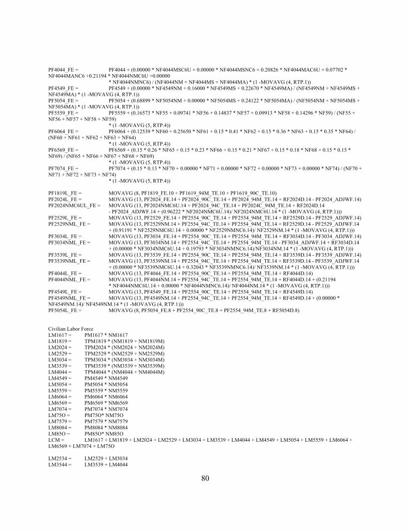
80

PF4044_FE = PF4044 + (0.00000 * NF4044MSC6U + 0.00000 * NF4044MSNC6 + 0.20826 * NF4044MAC6U + 0.07702 * NF4044MANC6 +0.21194 * NF4044NMC6U +0.00000 * NF4044NMNC6) / (NF4044NM + NF4044MS + NF4044MA) * (1 -MOVAVG (4, RTP.1)) PF4549_FE = PF4549 + (0.00000 * NF4549NM + 0.16000 * NF4549MS + 0.22670 * NF4549MA) / (NF4549NM + NF4549MS + NF4549MA) * (1 -MOVAVG (4, RTP.1)) PF5054_FE = PF5054 + (0.68899 * NF5054NM + 0.00000 * NF5054MS + 0.24122 * NF5054MA) / (NF5054NM + NF5054MS + NF5054MA) * (1 -MOVAVG (4, RTP.1)) PF5559_FE = PF5559 + (0.16573 * NF55 + 0.09741 * NF56 + 0.14837 * NF57 + 0.09913 * NF58 + 0.14296 * NF59) / (NF55 + NF56 + NF57 + NF58 + NF59) * (1 -MOVAVG (5, RTP.4)) PF6064_FE = PF6064 + (0.12539 * NF60 + 0.25650 * NF61 + 0.15 * 0.41 * NF62 + 0.15 * 0.36 * NF63 + 0.15 * 0.35 * NF64) / (NF60 + NF61 + NF62 + NF63 + NF64) * (1 -MOVAVG (5, RTP.4)) PF6569_FE = PF6569 + (0.15 * 0.26 * NF65 + 0.15 * 0.23 * NF66 + 0.15 * 0.21 * NF67 + 0.15 * 0.18 * NF68 + 0.15 * 0.15 * NF69) / (NF65 + NF66 + NF67 + NF68 + NF69) * (1 -MOVAVG (5, RTP.4)) PF7074_FE = PF7074 + (0.15 * 0.13 * NF70 + 0.00000 * NF71 + 0.00000 * NF72 + 0.00000 * NF73 + 0.00000 * NF74) / (NF70 + NF71 + NF72 + NF73 + NF74) * (1 -MOVAVG (5, RTP.4)) PF1819L_FE = MOVAVG (8, PF1819_FE.10 + PF1619_94M_TE.10 + PF1619_90C_TE.10) PF2024L_FE = MOVAVG (13, PF2024_FE.14 + PF2024_90C_TE.14 + PF2024_94M_TE.14 + RF2024D.14 - PF2024_ADJWF.14) PF2024NMC6UL_FE = MOVAVG (13, PF2024NMC6U.14 + PF2024_94C_TE.14 + PF2024C_94M_TE.14 + RF2024D.14 - PF2024_ADJWF.14 + (0.96222 * NF2024NMC6U.14)/ NF2024NMC6U.14 * (1 -MOVAVG (4, RTP.1))) PF2529L_FE = MOVAVG (13, PF2529_FE.14 + PF2554_90C_TE.14 + PF2554_94M_TE.14 + RF2529D.14 - PF2529_ADJWF.14) PF2529NML_FE = MOVAVG (13, PF2529NM.14 + PF2554_94C_TE.14 + PF2554_94M_TE.14 + RF2529D.14 - PF2529_ADJWF.14 + (0.91191 * NF2529NMC6U.14 + 0.00000 * NF2529NMNC6.14)/ NF2529NM.14 * (1 -MOVAVG (4, RTP.1))) PF3034L_FE = MOVAVG (13, PF3034_FE.14 + PF2554_90C_TE.14 + PF2554_94M_TE.14 + RF3034D.14 - PF3034_ADJWF.14) PF3034NML_FE = MOVAVG (13, PF3034NM.14 + PF2554_94C_TE.14 + PF2554_94M_TE.14 - PF3034_ADJWF.14 + RF3034D.14 + (0.00000 * NF3034NMC6U.14 + 0.19793 * NF3034NMNC6.14)/NF3034NM.14 * (1 -MOVAVG (4, RTP.1))) PF3539L_FE = MOVAVG (13, PF3539_FE.14 + PF2554_90C_TE.14 + PF2554_94M_TE.14 + RF3539D.14 - PF3539_ADJWF.14) PF3539NML_FE = MOVAVG (13, PF3539NM.14 + PF2554_94C_TE.14 + PF2554_94M_TE.14 + RF3539D.14 - PF3539_ADJWF.14 + (0.00000 * NF3539NMC6U.14 + 0.32043 * NF3539NMNC6.14)/ NF3539NM.14 * (1 -MOVAVG (4, RTP.1))) PF4044L_FE = MOVAVG (13, PF4044_FE.14 + PF2554_90C_TE.14 + PF2554_94M_TE.14 + RF4044D.14) PF4044NML_FE = MOVAVG (13, PF4044NM.14 + PF2554_94C_TE.14 + PF2554_94M_TE.14 + RF4044D.14 + (0.21194 * NF4044NMC6U.14 + 0.00000 * NF4044NMNC6.14)/ NF4044NM.14 * (1 -MOVAVG (4, RTP.1))) PF4549L_FE = MOVAVG (13, PF4549_FE.14 + PF2554_90C_TE.14 + PF2554_94M_TE.14 + RF4549D.14) PF4549NML_FE = MOVAVG (13, PF4549NM.14 + PF2554_94C_TE.14 + PF2554_94M_TE.14 + RF4549D.14 + (0.00000 * NF4549NM.14)/ NF4549NM.14 * (1 -MOVAVG (4, RTP.1))) PF5054L_FE = MOVAVG (8, PF5054_FE.8 + PF2554_90C_TE.8 + PF2554_94M_TE.8 + RF5054D.8) Civilian Labor Force LM1617 = PM1617 * NM1617 LM1819 = TPM1819 * (NM1819 + NM1819M) LM2024 = TPM2024 * (NM2024 + NM2024M) LM2529 = TPM2529 * (NM2529 + NM2529M) LM3034 = TPM3034 * (NM3034 + NM3034M) LM3539 = TPM3539 * (NM3539 + NM3539M) LM4044 = TPM4044 * (NM4044 + NM4044M) LM4549 = PM4549 * NM4549 LM5054 = PM5054 * NM5054 LM5559 = PM5559 * NM5559 LM6064 = PM6064 * NM6064 LM6569 = PM6569 * NM6569 LM7074 = PM7074 * NM7074 LM75O = PM75O* NM75O LM7579 = PM7579 * NM7579 LM8084 = PM8084 * NM8084 LM85O = PM85O* NM85O LCM = LM1617 + LM1819 + LM2024 + LM2529 + LM3034 + LM3539 + LM4044 + LM4549 + LM5054 + LM5559 + LM6064 + LM6569 + LM7074 + LM75O LM2534 = LM2529 + LM3034 LM3544 = LM3539 + LM4044

81

LM4554 = LM4549 + LM5054 LM5564 = LM5559 + LM6064 LM65O = LM6569 + LM7074 + LM75O Females LF1617 = PF1617 * NF1617 LF1819 = PF1819 * NF1819 LF2024 = PF2024 * NF2024 LF2529 = PF2529 * NF2529 LF3034 = PF3034 * NF3034 LF3539 = PF3539 * NF3539 LF4044 = PF4044 * NF4044 LF4549 = PF4549 * NF4549 LF5054 = PF5054 * NF5054 LF5559 = PF5559 * NF5559 LF6064 = PF6064 * NF6064 LF6569 = PF6569 * NF6569 LF7074 = PF7074 * NF7074 LF75O = PF75O* NF75O LF7579 = PF7579 * NF7579 LF8084 = PF8084 * NF8084 LF85O = PF85O* NF85O LCF = LF1617 + LF1819 + LF2024 + LF2529 + LF3034 + LF3539 + LF4044 + LF4549 + LF5054 + LF5559 + LF6064 + LF6569 + LF7074 + LF75O LF2534 = LF2529 + LF3034 LF3544 = LF3539 + LF4044 LF4554 = LF4549 + LF5054 LF5564 = LF5559 + LF6064 LF65O = LF6569 + LF7074 + LF75O LC = LCM + LCF DLF1617_FE = (PF1617_FE - PF1617) * NF1617 DLF1819_FE = (PF1819_FE - PF1819) * NF1819 DLF2024_FE = (PF2024_FE - PF2024) * NF2024 DLF2529_FE = (PF2529_FE - PF2529) * NF2529 DLF3034_FE = (PF3034_FE - PF3034) * NF3034 DLF3539_FE = (PF3539_FE - PF3539) * NF3539 DLF4044_FE = (PF4044_FE - PF4044) * NF4044 DLF4549_FE = (PF4549_FE - PF4549) * NF4549 DLF5054_FE = (PF5054_FE - PF5054) * NF5054 DLF5559_FE = (PF5559_FE - PF5559) * NF5559 DLF6064_FE = (PF6064_FE - PF6064) * NF6064 DLF6569_FE = (PF6569_FE - PF6569) * NF6569 DLF7074_FE = (PF7074_FE - PF7074) * NF7074 DLCF_FE = DLF1617_FE + DLF1819_FE + DLF2024_FE + DLF2529_FE + DLF3034_FE + DLF3539_FE + DLF4044_FE + DLF4549_FE + DLF5054_FE + DLF5559_FE + DLF6064_FE + DLF6569_FE + DLF7074_FE DLM1617_FE = (PM1617_FE - PM1617) * NM1617 DLM1819_FE = (TPM1819_FE - TPM1819) * (NM1819 + NM1819M) DLM2024_FE = (TPM2024_FE - TPM2024) * (NM2024 + NM2024M) DLM2529_FE = (TPM2529_FE - TPM2529) * (NM2529 + NM2529M) DLM3034_FE = (TPM3034_FE - TPM3034) * (NM3034 + NM3034M) DLM3539_FE = (TPM3539_FE - TPM3539) * (NM3539 + NM3539M) DLM4044_FE = (TPM4044_FE - TPM4044) * (NM4044 + NM4044M) DLM4549_FE = (PM4549_FE - PM4549) * NM4549 DLM5054_FE = (PM5054_FE - PM5054) * NM5054 DLM5559_FE = (PM5559_FE - PM5559) * NM5559 DLM6064_FE = (PM6064_FE - PM6064) * NM6064 DLM6569_FE = (PM6569_FE - PM6569) * NM6569 DLM7074_FE = (PM7074_FE - PM7074) * NM7074 DLCM_FE = DLM1617_FE + DLM1819_FE + DLM2024_FE + DLM2529_FE + DLM3034_FE + DLM3539_FE + DLM4044_FE + DLM4549_FE + DL

82

+ DLM6064_FE + DLM6569_FE + DLM7074_FE Unemployment Rates Totals MALES RM1617 = RM1617.1 + (-44.4261 * DIFF (RTP) - 2.1644 * DIFF (RTP.1) - 15.0910 * DIFF (RTP.2) - 27.8537 * DIFF (RTP.3)) * 50.00/44.05 RM1819 = RM1819.1 + (-47.9124 * DIFF (RTP) - 31.9746 * DIFF (RTP.1) - 11.6764 * DIFF (RTP.2) + 2.8763 * DIFF (RTP.3)) * 50.00/44.05 RM2024 = RM2024.1 + (-58.0805 * DIFF (RTP) - 14.6504 * DIFF (RTP.1) - 17.3907 * DIFF (RTP.2) - 8.3721 * DIFF (RTP.3)) * 50.00/44.05 RM2529 = RM2529.1 + (-42.4466 * DIFF (RTP) - 16.4626 * DIFF (RTP.1) - 12.0763 * DIFF (RTP.2) - 2.6912 * DIFF (RTP.3)) * 50.00/44.05 RM3034 = RM3034.1 + (-21.9947 * DIFF (RTP) - 14.3423 * DIFF (RTP.1) - 7.7729 * DIFF (RTP.2) - 4.5343 * DIFF (RTP.3)) * 50.00/44.05 RM3539 = RM3539.1 + (-25.1969 * DIFF (RTP) - 4.8918 * DIFF (RTP.1) - 11.6627 * DIFF (RTP.2) - 9.4142 * DIFF (RTP.3)) * 50.00/44.05 RM4044 = RM4044.1 + (-14.7303 * DIFF (RTP) - 12.8348 * DIFF (RTP.1) - 7.4111 * DIFF (RTP.2) - 6.4487 * DIFF (RTP.3)) * 50.00/44.05 RM4549 = RM4549.1 + (-18.1162 * DIFF (RTP) - 11.8573 * DIFF (RTP.1) - 7.3805 * DIFF (RTP.2) + 0.9708 * DIFF (RTP.3)) * 50.00/44.05 RM5054 = RM5054.1 + (-18.8477 * DIFF (RTP) - 11.0262 * DIFF (RTP.1) - 6.6450 * DIFF (RTP.2) - 4.7406 * DIFF (RTP.3)) * 50.00/44.05 RM5559 = RM5559.1 + (-22.8478 * DIFF (RTP) - 11.8787 * DIFF (RTP.1) + 0.6517 * DIFF (RTP.2) - 3.0202 * DIFF (RTP.3)) * 50.00/44.05 RM6064 = RM6064.1 + (1.4997 * DIFF (RTP) - 9.8165 * DIFF (RTP.1) + 0.4070 * DIFF (RTP.2) - 15.0849 * DIFF (RTP.3)) * 50.00/44.05 RM6569 = RM6569.1 + (-9.7596 * DIFF (RTP) + 11.8572 * DIFF (RTP.1) - 18.3547 * DIFF (RTP.2) + 6.1962 * DIFF (RTP.3)) *

50.00/44.05 RM7074 = RM7074.1 + (19.6295 * DIFF (RTP) - 12.5956 * DIFF (RTP.1) - 27.9350 * DIFF (RTP.2) + 6.5664 * DIFF (RTP.3)) *

50.00/44.05 RM75O = RM75O.1 + (- 5.5101 * DIFF (RTP) - 18.5248 * DIFF (RTP.1) - 17.9157 * DIFF (RTP.2) + 23.5855 * DIFF (RTP.3)) *

50.00/44.05 FEMALES RF1617 = RF1617.1 + (-20.9377 * DIFF (RTP) - 3.4543 * DIFF (RTP.1) - 32.5068 * DIFF (RTP.2) - 8.8148 * DIFF (RTP.3)) * 50.00/44.05 RF1819 = RF1819.1 + (-39.2646 * DIFF (RTP) - 5.1023 * DIFF (RTP.1) + 3.6786 * DIFF (RTP.2) - 27.3641 * DIFF (RTP.3)) * 50.00/44.05 RF2024 = RF2024.1 + (-26.8299 * DIFF (RTP) - 11.1330 * DIFF (RTP.1) - 11.4402 * DIFF (RTP.2) - 4.0048 * DIFF (RTP.3)) * 50.00/44.05 RF2529 = RF2529.1 + (-14.8770 * DIFF (RTP) - 8.8852 * DIFF (RTP.1) - 12.9537 * DIFF (RTP.2) - 0.6317 * DIFF (RTP.3)) * 50.00/44.05 RF3034 = RF3034.1 + (-10.3084 * DIFF (RTP) - 0.6837 * DIFF (RTP.1) - 18.4113 * DIFF (RTP.2) - 2.0406 * DIFF (RTP.3)) * 50.00/44.05 RF3539 = RF3539.1 + (-17.8370 * DIFF (RTP) - 2.3913 * DIFF (RTP.1) - 6.8006 * DIFF (RTP.2) - 5.0086 * DIFF (RTP.3)) * 50.00/44.05 RF4044 = RF4044.1 + (-6.9101 * DIFF (RTP) - 9.4509 * DIFF (RTP.1) - 3.6043 * DIFF (RTP.2) - 1.8449 * DIFF (RTP.3)) * 50.00/44.05 RF4549 = RF4549.1 + (-1.6363 * DIFF (RTP) - 19.4549 * DIFF (RTP.1) + 10.7519 * DIFF (RTP.2) - 8.6682 * DIFF (RTP.3)) * 50.00/44.05 RF5054 = RF5054.1 + (-12.0818 * DIFF (RTP) + 0.3229 * DIFF (RTP.1) - 15.0622 * DIFF (RTP.2) - 3.0337 * DIFF (RTP.3)) * 50.00/44.05 RF5559 = RF5559.1 + (2.7183 * DIFF (RTP) - 9.8009 * DIFF (RTP.1) - 6.1773 * DIFF (RTP.2) - 6.3238 * DIFF (RTP.3)) * 50.00/44.05 RF6064 = RF6064.1 + (-11.7151 * DIFF (RTP) - 1.9990 * DIFF (RTP.1) - 3.1837 * DIFF (RTP.2) - 10.6383 * DIFF (RTP.3)) * 50.00/44.05 RF6569 = RF6569.1 + (-8.7042 * DIFF (RTP.2) - 4.6979 * DIFF (RTP.3)) * 50.00/44.05 RF7074 = RF7074.1 + (0.2827 * DIFF (RTP.2) - 14.1285 * DIFF (RTP.3)) * 50.00/44.05 RF75O = RF75O.1 + (-11.6993 * DIFF (RTP) + 13.5790 * DIFF (RTP.1) + 8.9530 * DIFF (RTP.2) - 22.2054 * DIFF (RTP.3)) * 50.00/44.05 EQ RUM = (RM1617 * LM1617 + RM1819 * LM1819 + RM2024 * LM2024 + RM2529 * LM2529 + RM3034 * LM3034 + RM3539 * LM3539 + RM4044 * LM4044 + RM4549 * LM4549

83

+ RM5054 * LM5054 + RM5559 * LM5559 + RM6064 * LM6064 + RM6569 * LM6569 + RM7074 * LM7074 + RM75O * LM75O)/ LCM EQ RUF = (RF1617 * LF1617 + RF1819 * LF1819 + RF2024 * LF2024 + RF2529 * LF2529 + RF3034 * LF3034 + RF3539 * LF3539 + RF4044 * LF4044 + RF4549 * LF4549 + RF5054 * LF5054 + RF5559 * LF5559 + RF6064 * LF6064 + RF6569 * LF6569 + RF7074 * LF7074 + RF75O * LF75O)/ LCF EQ RU = (RUM * LCM + RUF * LCF) / LC

84

2.2 U.S. Earnings (USEAR) Annual Employment Equations Class of Worker Nonagricultural Wage Workers Private Household Workers EF1617NAWPH = MAX (0.001, -0.20802 * RTP - 0.40988 * RTP.1 + 0.01015 + 61.2465 * 1/YEAR - 0.00965 * MINW/CPIW_U + 0.01561 * NU10/NF1617 - 0.13398) * EF1617 EF1819NAWPH = MAX (0.001, -0.03363 * RTP - 0.12989 * RTP.1 - 0.00661 + 8.44701 * 1/YEAR - 0.00539 * MINW/CPIW_U + 0.00345 * NU10/NF1819 + 0.07597) * EF1819 EF2024NAWPH = MAX (0.001, -0.18707 * MOVAVG (5, RTP) - 0.00223 + 2.12060 * 1/YEAR + 0.00820 * NU10/NF2024 + 0.14537) * EF2024 EF2534NAWPH = MAX (0.001, 0.01874 * RTP - 0.04167 * MOVAVG (5, RTP.1) - 0.00090 + 1.55167 * 1/YEAR + 0.01021 * NU10/NF2534 - 0.00170) * EF2534 EF3544NAWPH = (0.00622 * RTP - 0.06062 * MOVAVG (5, RTP.1) + 0.00008 + 0.29372 * MOVAVG (3, EF2534NAWPH.9/EF2534.9) + 0.06187) * EF3544 EF4554NAWPH = (0.02788 * RTP - 0.10996 * MOVAVG (5, RTP.1) - 0.00349 + 0.53068 * MOVAVG (3, EF3544NAWPH.9/EF3544.9) + 0.08883) * EF4554 EF5564NAWPH = (0.05939 * RTP - 0.10618 * MOVAVG (2, RTP.1) - 0.00579 + 0.66195 * MOVAVG (3, EF4554NAWPH.9/EF4554.9) + 0.05966) * EF5564 EF65ONAWPH = (0.22642 * RTP - 0.02069 + 0.33505 * MOVAVG (3, EF5564NAWPH.9) - 0.19707) EM1617NAWPH = MAX (0.001, -0.05284 * RTP - 0.17833 * RTP.1 - 0.00768 + 9.19738 * 1/YEAR - 0.00588 * MINW/CPIW_U + 0.16862) * EM1617 EM1819NAWPH = MAX (0.001, -0.07122 * RTP - 0.03737 * RTP.1 - 0.00282 + 3.76796 * 1/YEAR - 0.00499 * MINW/CPIW_U + 0.08727) * EM1819 EM2024NAWPH = MAX (0.001, -0.00450 * RTP - 0.02345 * RTP.1 - 0.00113 - 0.00057 * MINW/CPIW_U + 0.03265) * EM2024 EM2534NAWPH = MAX (0.001, -0.00490 * RTP.1 - 0.00054 - 0.00051 * MINW/CPIW_U + 0.00789) * EM2534 EM3544NAWPH = (-0.00446 * RTP.1 - 0.00041 - 0.00053 * MINW/CPIW_U + 0.00726) * EM3544 EM4554NAWPH = (-0.00039 + 0.00129) * EM4554 EM5564NAWPH = (-0.00015 + 0.00200) * EM5564 EM65ONAWPH = (-0.00679 + 0.64405 * MOVAVG (3, EM5564NAWPH.9) + 0.00231) Government Other Self-employed EF1617NAS = (0.12015 * RTP.1 - 0.10551) * EF1617 Ordinary Least Squares ANNUAL data for 5 periods from 2000 to 2004 Date: 9 NOV 2005 ef1617nas/ef1617 = 0.12015 * rtp.1 - 0.10551 (1.96868) (1.73441) Sum Sq 0.0000 Std Error 0.0030 LHS Mean 0.0142 R-Squared 0.5637 R Bar Squared 0.4182 F-stat 1, 3 3.8757 D.W. (1) 1.5620 D.W. (2) 2.3626 EF1819NAS = (0.11184 * RTP.1 - 0.10241) * EF1819 Ordinary Least Squares ANNUAL data for 5 periods from 2000 to 2004

85

Date: 9 NOV 2005 ef1819nas/ef1819 = 0.11184 * rtp.1 - 0.10241 (2.99537) (2.75170) Sum Sq 0.0000 Std Error 0.0018 LHS Mean 0.0090 R-Squared 0.7494 R Bar Squared 0.6659 F-STAT 1, 3 8.9722 D.W. (1) 3.2586 D.W. (2) 0.9766 EF2024NAS = (0.08908 * RTP.1 - 0.07176) * EF2024 Ordinary Least Squares ANNUAL data for 5 periods from 2000 to 2004 Date: 9 NOV 2005 ef2024nas/ef2024 = 0.08908 * rtp.1 - 0.07176 (2.54605) (2.05763) Sum Sq 0.0000 Std Error 0.0017 LHS Mean 0.0170 R-Squared 0.6836 R Bar Squared 0.5782 F-STAT 1, 3 6.4824 D.W. (1) 2.6600 D.W. (2) 1.5247 EF2534NAS = (0.00906 * RTP.1 + 0.03539) * EF2534 Ordinary Least Squares ANNUAL data for 5 periods from 2000 to 2004 Date: 9 NOV 2005 ef2534nas/ef2534 = 0.00906 * rtp.1 + 0.03539 (0.34277) (1.34366) Sum Sq 0.0000 Std Error 0.0013 LHS Mean 0.0444 R-Squared 0.0377 R Bar Squared 0.2831 F-STAT 1, 3 0.1175 D.W. (1) 3.0818 D.W. (2) 1.1094 EF3544NAS = (-0.01869 * RTP.1 + 0.08087) * EF3544 Ordinary Least Squares ANNUAL data for 5 periods from 2000 to 2004 Date: 9 NOV 2005 ef3544nas/ef3544 = -0.01869 * rtp.1 + 0.08087 (0.70565) (3.06320) Sum Sq 0.0000 Std Error 0.0013 LHS Mean 0.0622 R-Squared 0.1424 R Bar Squared 0.1435 F-STAT 1, 3 0.4979 D.W. (1) 2.2440 D.W. (2) 2.1852 EF4554NAS = (0.07232 * RTP.1 - 0.00701) * EF4554

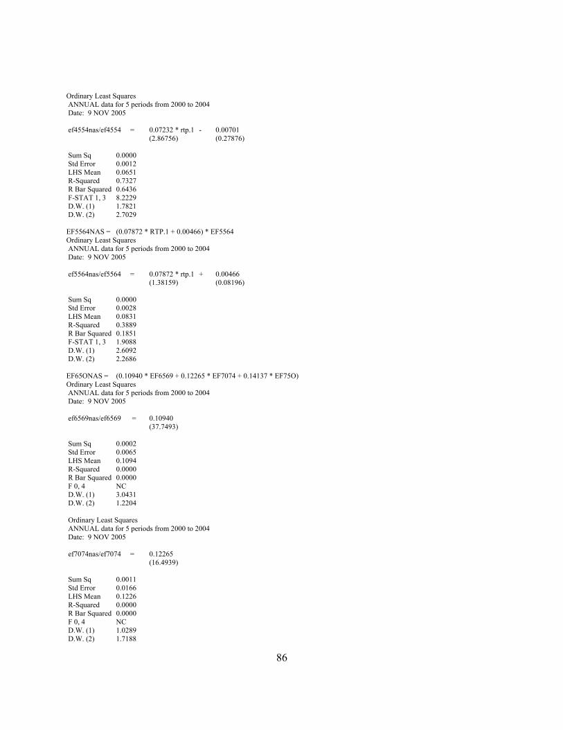
86

Ordinary Least Squares ANNUAL data for 5 periods from 2000 to 2004 Date: 9 NOV 2005 ef4554nas/ef4554 = 0.07232 * rtp.1 - 0.00701 (2.86756) (0.27876) Sum Sq 0.0000 Std Error 0.0012 LHS Mean 0.0651 R-Squared 0.7327 R Bar Squared 0.6436 F-STAT 1, 3 8.2229 D.W. (1) 1.7821 D.W. (2) 2.7029 EF5564NAS = (0.07872 * RTP.1 + 0.00466) * EF5564 Ordinary Least Squares ANNUAL data for 5 periods from 2000 to 2004 Date: 9 NOV 2005 ef5564nas/ef5564 = 0.07872 * rtp.1 + 0.00466 (1.38159) (0.08196) Sum Sq 0.0000 Std Error 0.0028 LHS Mean 0.0831 R-Squared 0.3889 R Bar Squared 0.1851 F-STAT 1, 3 1.9088 D.W. (1) 2.6092 D.W. (2) 2.2686 EF65ONAS = (0.10940 * EF6569 + 0.12265 * EF7074 + 0.14137 * EF75O) Ordinary Least Squares ANNUAL data for 5 periods from 2000 to 2004 Date: 9 NOV 2005 ef6569nas/ef6569 = 0.10940 (37.7493) Sum Sq 0.0002 Std Error 0.0065 LHS Mean 0.1094 R-Squared 0.0000 R Bar Squared 0.0000 F 0, 4 NC D.W. (1) 3.0431 D.W. (2) 1.2204 Ordinary Least Squares ANNUAL data for 5 periods from 2000 to 2004 Date: 9 NOV 2005 ef7074nas/ef7074 = 0.12265 (16.4939) Sum Sq 0.0011 Std Error 0.0166 LHS Mean 0.1226 R-Squared 0.0000 R Bar Squared 0.0000 F 0, 4 NC D.W. (1) 1.0289 D.W. (2) 1.7188

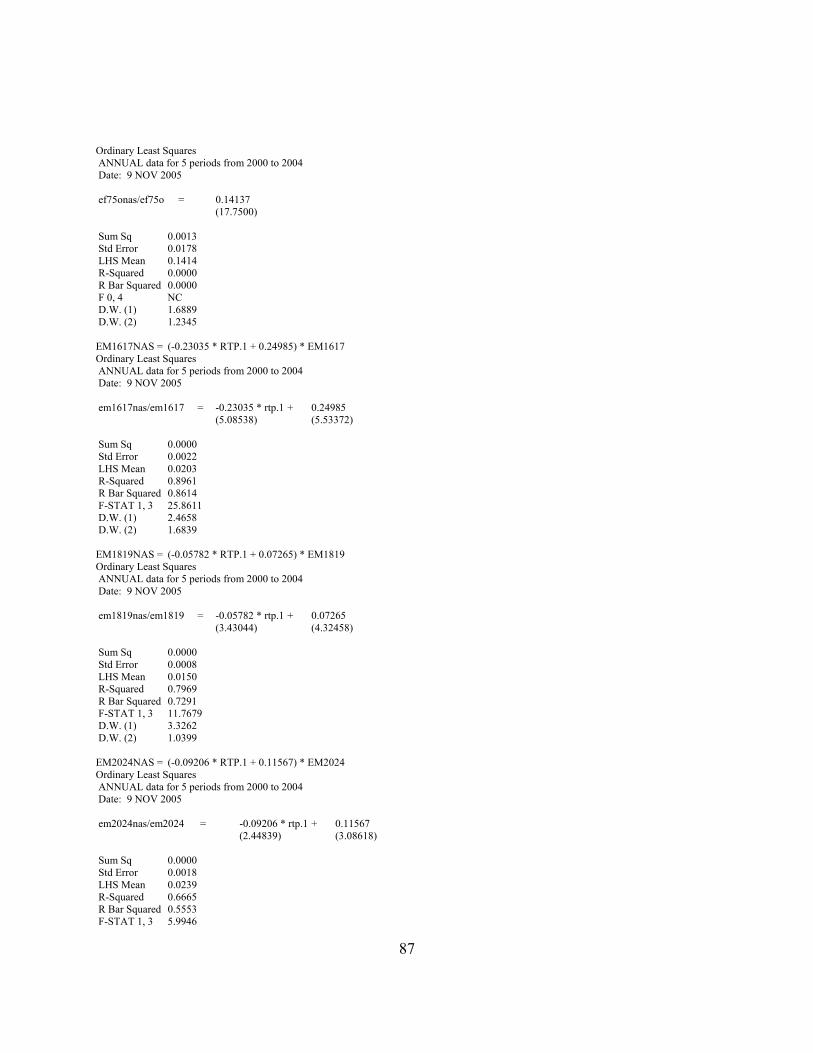
87

Ordinary Least Squares ANNUAL data for 5 periods from 2000 to 2004 Date: 9 NOV 2005 ef75onas/ef75o = 0.14137 (17.7500) Sum Sq 0.0013 Std Error 0.0178 LHS Mean 0.1414 R-Squared 0.0000 R Bar Squared 0.0000 F 0, 4 NC D.W. (1) 1.6889 D.W. (2) 1.2345 EM1617NAS = (-0.23035 * RTP.1 + 0.24985) * EM1617 Ordinary Least Squares ANNUAL data for 5 periods from 2000 to 2004 Date: 9 NOV 2005 em1617nas/em1617 = -0.23035 * rtp.1 + 0.24985 (5.08538) (5.53372) Sum Sq 0.0000 Std Error 0.0022 LHS Mean 0.0203 R-Squared 0.8961 R Bar Squared 0.8614 F-STAT 1, 3 25.8611 D.W. (1) 2.4658 D.W. (2) 1.6839 EM1819NAS = (-0.05782 * RTP.1 + 0.07265) * EM1819 Ordinary Least Squares ANNUAL data for 5 periods from 2000 to 2004 Date: 9 NOV 2005 em1819nas/em1819 = -0.05782 * rtp.1 + 0.07265 (3.43044) (4.32458) Sum Sq 0.0000 Std Error 0.0008 LHS Mean 0.0150 R-Squared 0.7969 R Bar Squared 0.7291 F-STAT 1, 3 11.7679 D.W. (1) 3.3262 D.W. (2) 1.0399 EM2024NAS = (-0.09206 * RTP.1 + 0.11567) * EM2024 Ordinary Least Squares ANNUAL data for 5 periods from 2000 to 2004 Date: 9 NOV 2005 em2024nas/em2024 = -0.09206 * rtp.1 + 0.11567 (2.44839) (3.08618) Sum Sq 0.0000 Std Error 0.0018 LHS Mean 0.0239 R-Squared 0.6665 R Bar Squared 0.5553 F-STAT 1, 3 5.9946

88

D.W. (1) 2.1493 D.W. (2) 1.7046 EM2534NAS = (-0.09661 * RTP.1 + 0.14843) * EM2534 Ordinary Least Squares ANNUAL data for 5 periods from 2000 to 2004 Date: 9 NOV 2005 em2534nas/em2534 = -0.09661 * rtp.1 + 0.14843 (2.81478) (4.33847) Sum Sq 0.0000 Std Error 0.0017 LHS Mean 0.0522 R-Squared 0.7254 R Bar Squared 0.6338 F-STAT 1, 3 7.9230 D.W. (1) 1.8300 D.W. (2) 2.9632 EM3544NAS = (0.02739 * RTP.1 + 0.05236) * EM3544 Ordinary Least Squares ANNUAL data for 5 periods from 2000 to 2004 Date: 9 NOV 2005 em3544nas/em3544 = 0.02739 * rtp.1 + 0.05236 (0.61129) (1.17241) Sum Sq 0.0000 Std Error 0.0022 LHS Mean 0.0797 R-Squared 0.1108 R Bar Squared 0.1857 F-STAT 1, 3 0.3737 D.W. (1) 2.5508 D.W. (2) 2.2676 EM4554NAS = (0.06217 * RTP.1 + 0.03411) * EM4554 Ordinary Least Squares ANNUAL data for 5 periods from 2000 to 2004 Date: 9 NOV 2005 em4554nas/em4554 = 0.06217 * rtp.1 + 0.03411 (1.91738) (1.05544) Sum Sq 0.0000 Std Error 0.0016 LHS Mean 0.0961 R-Squared 0.5507 R Bar Squared 0.4009 F-STAT 1, 3 3.6764 D.W. (1) 2.5497 D.W. (2) 1.5554 EM5564NAS = (-0.04776 * RTP.1 + 0.16626) * EM5564 Ordinary Least Squares ANNUAL data for 5 periods from 2000 to 2004 Date: 9 NOV 2005 em5564nas/em5564 = -0.04776 * rtp.1 + 0.16626 (0.60480) (2.11226) Sum Sq 0.0000 Std Error 0.0039 LHS Mean 0.1187

89

R-Squared 0.1087 R Bar Squared 0.1884 F-STAT 1, 3 0.3658 D.W. (1) 2.9234 D.W. (2) 1.9432 EM65ONAS = (0.16527 * EM6569 + 0.17798 * EM7074 + 0.19058 * EM75O) Ordinary Least Squares ANNUAL data for 5 periods from 2000 to 2004 Date: 9 NOV 2005 em6569nas/em6569 = 0.16527 (53.9126) Sum Sq 0.0002 Std Error 0.0069 LHS Mean 0.1653 R-Squared 0.0000 R Bar Squared 0.0000 F-stat 0, 4 NC D.W. (1) 1.7716 D.W. (2) 2.9645 Ordinary Least Squares ANNUAL data for 5 periods from 2000 to 2004 Date: 9 NOV 2005 em7074nas/em7074 = 0.17798 (22.9265) Sum Sq 0.0012 Std Error 0.0174 LHS Mean 0.1780 R-Squared 0.0000 R Bar Squared 0.0000 F-stat 0, 4 NC D.W. (1) 1.7116 D.W. (2) 2.1991 Ordinary Least Squares ANNUAL data for 5 periods from 2000 to 2004 Date: 9 NOV 2005 em75onas/em75o = 0.19058 (20.1892) Sum Sq 0.0018 Std Error 0.0211 LHS Mean 0.1906 R-Squared 0.0000 R Bar Squared 0.0000 F-stat 0, 4 NC D.W. (1) 2.7330 D.W. (2) 0.9992 Unpaid Family Workers EF1617NAU = 0.00012 * ENAS EF1819NAU = 0.00025 * ENAS EF2024NAU = 0.00024 * ENAS EF2534NAU = 0.00117 * ENAS EF3544NAU = 0.00218 * ENAS EF4554NAU = 0.00226 * ENAS EF5564NAU = 0.00083 * ENAS EF65ONAU = (0.00027 + 0.00021 + 0.00008) * ENAS

90

EM1617NAU = 0.00028 * ENAS EM1819NAU = 0.00033 * ENAS EM2024NAU = 0.00050 * ENAS EM2534NAU = 0.00044 * ENAS EM3544NAU = 0.00043 * ENAS EM4554NAU = 0.00052 * ENAS EM5564NAU = 0.00037 * ENAS EM65ONAU = (0.00023 + 0.00010 + 0.00011) * ENAS Agricultural Wage Workers EM1617AW = EAW * (-0.00594 - 0.09353 * RTP + 5.28754 * EM1617/E + 0.08116) EM1819AW = EAW * (-0.00131 - 0.18120 * RTP + 3.87151 * EM1819/E + 0.16636) EM2024AW = EAW * (-0.00664 + 0.10493 * RTP + 2.00153 * EM2024/E - 0.08191) EM2534AW = EAW * (-0.02065 + 0.38358 * RTP - 0.98380 * EM2534/E + 0.00751) EM3544AW = EAW * (0.00402 - 0.15663 * RTP + 1.72119 * EM3544/E + 0.05679) EM4554AW = EAW * (0.00834 + 0.03746 * RTP + 0.46522 * EM4554/E + 0.00144) EM5564AW = EAW * (-0.00655 + 0.03521 * RTP + 0.46852 * EM5564/E - 0.00037) EM65OAW = EAW * (-0.00114 + 0.07640 * RTP + 3.25911 * EM65O/E - 0.10058) EF1617AW = EAW * (-0.00055 - 0.05470 * RTP + 1.41760 * EF1617/E + 0.04979) EF1819AW = EAW * (0.00102 - 0.07375 * RTP + 0.78394 * EF1819/E + 0.07226) EF2024AW = EAW * (0.00112 - 0.05971 * RTP + 0.57256 * EF2024/E + 0.05907) EF2534AW = EAW * (0.00623 + 0.08868 * RTP + 1.00897 * EF2534/E - 0.15142) EF3544AW = EAW * (0.00687 - 0.00259 * RTP + 0.51319 * EF3544/E - 0.00937) EF4554AW = EAW * (0.00185 + 0.08747 * RTP + 0.28022 * EF4554/E - 0.08053) EF5564AW = EAW * (-0.00140 - 0.03001 * RTP - 0.59383 * EF5564/E + 0.07088) EF65OAW = EAW * (0.00096 + 0.06768 * RTP + 1.04213 * EF65O/E - 0.07359) Self-employed EM1617AS = NM1617 * (0.00528 + 0.00404) EM1819AS = NM1819 * (0.00309 + 0.28448 * EA / (NM16O+ NF16O) - 0.00165) EM2024AS = NM2024 * (-0.00181 + 0.97958 * EA / (NM16O+ NF16O) - 0.01093) EM2534AS = NM2534 * (-0.00263 + 1.23186 * EA / (NM16O+ NF16O) - 0.01021) EM3544AS = NM3544 * (-0.00151 + 1.66765 * EA / (NM16O+ NF16O) - 0.01450) EM4554AS = NM4554 * (-0.00381 + 2.86654 * EA / (NM16O+ NF16O) - 0.03175) EM5564AS = NM5564 * (-0.00460 + 2.78817 * EA / (NM16O+ NF16O) - 0.02398) EM65OAS = NM65O * (0.00079 + 1.76904 * EA / (NM16O+ NF16O) - 0.01437) EF1617AS = NF1617 * (0.00181 + 0.00030) EF1819AS = EM1819AS * (-0.02393 + 0.63672 * RTP + 0.98791 * EF1819/EM1819 - 1.43926) EF2024AS = EM2024AS * (0.07353 - 0.40207 * RTP + 0.57572 * EF2024/EM2024 - 0.01117) EF2534AS = EM2534AS * (0.16575 + 0.16967 * RTP + 0.55503 * EF2534/EM2534 - 0.43412) EF3544AS = EM3544AS * (0.15848 + 0.37839 * RTP + 0.37764 * EF3544/EM3544 - 0.45362) EF4554AS = EM4554AS * (0.21947 + 0.29497 * RTP + 0.58974 * EF4554/EM4554 - 0.51966) EF5564AS = EM5564AS * (0.20892 + 0.36294 * RTP + 0.65320 * EF5564/EM5564 - 0.66626) EF65OAS = EM65OAS * (0.16242 + 0.54916 * RTP + 0.06199 * EF65O/EM65O - 0.47556) Unpaid Family Workers EF1617AU = 0.002 EF1819AU = 0.001 EF2024AU = 0.001 EF2534AU = 0.003 EF3544AU = 0.004 EF4554AU = 0.005 EF5564AU = 0.003 EF65OAU = 0.001 EM1617AU = 0.006 EM1819AU = 0.005

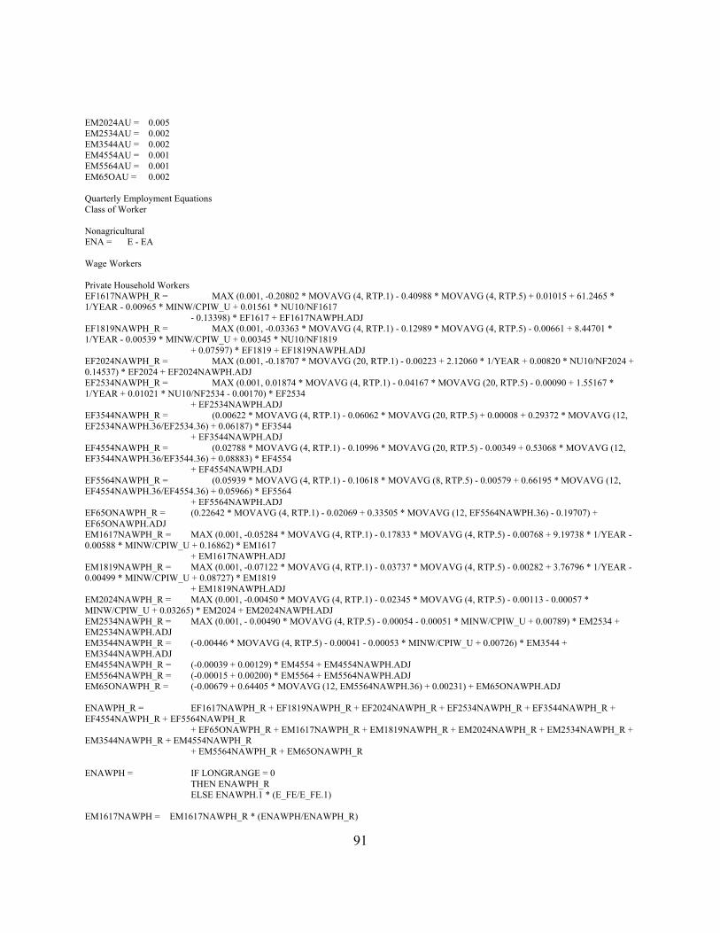
91

EM2024AU = 0.005 EM2534AU = 0.002 EM3544AU = 0.002 EM4554AU = 0.001 EM5564AU = 0.001 EM65OAU = 0.002 Quarterly Employment Equations Class of Worker Nonagricultural ENA = E - EA Wage Workers Private Household Workers EF1617NAWPH_R = MAX (0.001, -0.20802 * MOVAVG (4, RTP.1) - 0.40988 * MOVAVG (4, RTP.5) + 0.01015 + 61.2465 * 1/YEAR - 0.00965 * MINW/CPIW_U + 0.01561 * NU10/NF1617 - 0.13398) * EF1617 + EF1617NAWPH.ADJ EF1819NAWPH_R = MAX (0.001, -0.03363 * MOVAVG (4, RTP.1) - 0.12989 * MOVAVG (4, RTP.5) - 0.00661 + 8.44701 * 1/YEAR - 0.00539 * MINW/CPIW_U + 0.00345 * NU10/NF1819 + 0.07597) * EF1819 + EF1819NAWPH.ADJ EF2024NAWPH_R = MAX (0.001, -0.18707 * MOVAVG (20, RTP.1) - 0.00223 + 2.12060 * 1/YEAR + 0.00820 * NU10/NF2024 + 0.14537) * EF2024 + EF2024NAWPH.ADJ EF2534NAWPH_R = MAX (0.001, 0.01874 * MOVAVG (4, RTP.1) - 0.04167 * MOVAVG (20, RTP.5) - 0.00090 + 1.55167 * 1/YEAR + 0.01021 * NU10/NF2534 - 0.00170) * EF2534 + EF2534NAWPH.ADJ EF3544NAWPH_R = (0.00622 * MOVAVG (4, RTP.1) - 0.06062 * MOVAVG (20, RTP.5) + 0.00008 + 0.29372 * MOVAVG (12, EF2534NAWPH.36/EF2534.36) + 0.06187) * EF3544 + EF3544NAWPH.ADJ EF4554NAWPH_R = (0.02788 * MOVAVG (4, RTP.1) - 0.10996 * MOVAVG (20, RTP.5) - 0.00349 + 0.53068 * MOVAVG (12, EF3544NAWPH.36/EF3544.36) + 0.08883) * EF4554 + EF4554NAWPH.ADJ EF5564NAWPH_R = (0.05939 * MOVAVG (4, RTP.1) - 0.10618 * MOVAVG (8, RTP.5) - 0.00579 + 0.66195 * MOVAVG (12, EF4554NAWPH.36/EF4554.36) + 0.05966) * EF5564 + EF5564NAWPH.ADJ EF65ONAWPH_R = (0.22642 * MOVAVG (4, RTP.1) - 0.02069 + 0.33505 * MOVAVG (12, EF5564NAWPH.36) - 0.19707) + EF65ONAWPH.ADJ EM1617NAWPH_R = MAX (0.001, -0.05284 * MOVAVG (4, RTP.1) - 0.17833 * MOVAVG (4, RTP.5) - 0.00768 + 9.19738 * 1/YEAR - 0.00588 * MINW/CPIW_U + 0.16862) * EM1617 + EM1617NAWPH.ADJ EM1819NAWPH_R = MAX (0.001, -0.07122 * MOVAVG (4, RTP.1) - 0.03737 * MOVAVG (4, RTP.5) - 0.00282 + 3.76796 * 1/YEAR - 0.00499 * MINW/CPIW_U + 0.08727) * EM1819 + EM1819NAWPH.ADJ EM2024NAWPH_R = MAX (0.001, -0.00450 * MOVAVG (4, RTP.1) - 0.02345 * MOVAVG (4, RTP.5) - 0.00113 - 0.00057 * MINW/CPIW_U + 0.03265) * EM2024 + EM2024NAWPH.ADJ EM2534NAWPH_R = MAX (0.001, - 0.00490 * MOVAVG (4, RTP.5) - 0.00054 - 0.00051 * MINW/CPIW_U + 0.00789) * EM2534 + EM2534NAWPH.ADJ EM3544NAWPH_R = (-0.00446 * MOVAVG (4, RTP.5) - 0.00041 - 0.00053 * MINW/CPIW_U + 0.00726) * EM3544 + EM3544NAWPH.ADJ EM4554NAWPH_R = (-0.00039 + 0.00129) * EM4554 + EM4554NAWPH.ADJ EM5564NAWPH_R = (-0.00015 + 0.00200) * EM5564 + EM5564NAWPH.ADJ EM65ONAWPH_R = (-0.00679 + 0.64405 * MOVAVG (12, EM5564NAWPH.36) + 0.00231) + EM65ONAWPH.ADJ ENAWPH_R = EF1617NAWPH_R + EF1819NAWPH_R + EF2024NAWPH_R + EF2534NAWPH_R + EF3544NAWPH_R + EF4554NAWPH_R + EF5564NAWPH_R + EF65ONAWPH_R + EM1617NAWPH_R + EM1819NAWPH_R + EM2024NAWPH_R + EM2534NAWPH_R + EM3544NAWPH_R + EM4554NAWPH_R + EM5564NAWPH_R + EM65ONAWPH_R ENAWPH = IF LONGRANGE = 0 THEN ENAWPH_R ELSE ENAWPH.1 * (E_FE/E_FE.1) EM1617NAWPH = EM1617NAWPH_R * (ENAWPH/ENAWPH_R)

92

EM1819NAWPH = EM1819NAWPH_R * (ENAWPH/ENAWPH_R) EM2024NAWPH = EM2024NAWPH_R * (ENAWPH/ENAWPH_R) EM2534NAWPH = EM2534NAWPH_R * (ENAWPH/ENAWPH_R) EM3544NAWPH = EM3544NAWPH_R * (ENAWPH/ENAWPH_R) EM4554NAWPH = EM4554NAWPH_R * (ENAWPH/ENAWPH_R) EM5564NAWPH = EM5564NAWPH_R * (ENAWPH/ENAWPH_R) EM65ONAWPH = EM65ONAWPH_R * (ENAWPH/ENAWPH_R) EF1617NAWPH = EF1617NAWPH_R * (ENAWPH/ENAWPH_R) EF1819NAWPH = EF1819NAWPH_R * (ENAWPH/ENAWPH_R) EF2024NAWPH = EF2024NAWPH_R * (ENAWPH/ENAWPH_R) EF2534NAWPH = EF2534NAWPH_R * (ENAWPH/ENAWPH_R) EF3544NAWPH = EF3544NAWPH_R * (ENAWPH/ENAWPH_R) EF4554NAWPH = EF4554NAWPH_R * (ENAWPH/ENAWPH_R) EF5564NAWPH = EF5564NAWPH_R * (ENAWPH/ENAWPH_R) EF65ONAWPH = EF65ONAWPH_R * (ENAWPH/ENAWPH_R) EFNAWPH = EF1617NAWPH + EF1819NAWPH + EF2024NAWPH + EF2534NAWPH + EF3544NAWPH + EF4554NAWPH + EF5564NAWPH + EF65ONAWPH EMNAWPH = EM1617NAWPH + EM1819NAWPH + EM2024NAWPH + EM2534NAWPH + EM3544NAWPH + EM4554NAWPH + EM5564NAWPH + EM65ONAWPH Government Other Self-employed EF1617NAS_R = (0.12015 * RTP.1 - 0.10551) * EF1617 + EF1617NAS.ADJ EF1819NAS_R = (0.11184 * RTP.1 - 0.10241) * EF1819 + EF1819NAS.ADJ EF2024NAS_R = (0.08908 * RTP.1 - 0.07176) * EF2024 + EF2024NAS.ADJ EF2534NAS_R = (0.00906 * RTP.1 + 0.03539) * EF2534 + EF2534NAS.ADJ EF3544NAS_R = (-0.01869 * RTP.1 + 0.08087) * EF3544 + EF3544NAS.ADJ EF4554NAS_R = (0.07232 * RTP.1 - 0.00701) * EF4554 + EF4554NAS.ADJ EF5564NAS_R = (0.07872 * RTP.1 + 0.00466) * EF5564 + EF5564NAS.ADJ EF65ONAS_R = (0.10940 * EF6569 + 0.12265 * EF7074 + 0.14137 * EF75O) + EF65ONAS.ADJ EM1617NAS_R = (-0.23035 * RTP.1 + 0.24985) * EM1617 + EM1617NAS.ADJ EM1819NAS_R = (-0.05782 * RTP.1 + 0.07265) * EM1819 + EM1819NAS.ADJ EM2024NAS_R = (-0.09206 * RTP.1 + 0.11567) * EM2024 + EM2024NAS.ADJ EM2534NAS_R = (-0.09661 * RTP.1 + 0.14843) * EM2534 + EM2534NAS.ADJ EM3544NAS_R = (0.02739 * RTP.1 + 0.05236) * EM3544 + EM3544NAS.ADJ EM4554NAS_R = (0.06217 * RTP.1 + 0.03411) * EM4554 + EM4554NAS.ADJ EM5564NAS_R = (-0.04776 * RTP.1 + 0.16626) * EM5564 + EM5564NAS.ADJ EM65ONAS_R = (0.16527 * EM6569 + 0.17798 * EM7074 + 0.19058 * EM75O) + EM65ONAS.ADJ ENAS_R = EF1617NAS_R + EF1819NAS_R + EF2024NAS_R + EF2534NAS_R + EF3544NAS_R + EF4554NAS_R + EF5564NAS_R + EF65ONAS_R + EM1617NAS_R + EM1819NAS_R + EM2024NAS_R + EM2534NAS_R + EM3544NAS_R + EM4554NAS_R + EM5564NAS_R + EM65ONAS_R ENAS = IF LONGRANGE = 0 THEN ENAS_R ELSE ENA * (ENAS.1/ENA.1) EM1617NAS = EM1617NAS_R * (ENAS/ENAS_R) EM1819NAS = EM1819NAS_R * (ENAS/ENAS_R) EM2024NAS = EM2024NAS_R * (ENAS/ENAS_R) EM2534NAS = EM2534NAS_R * (ENAS/ENAS_R) EM3544NAS = EM3544NAS_R * (ENAS/ENAS_R) EM4554NAS = EM4554NAS_R * (ENAS/ENAS_R) EM5564NAS = EM5564NAS_R * (ENAS/ENAS_R) EM65ONAS = EM65ONAS_R * (ENAS/ENAS_R) EF1617NAS = EF1617NAS_R * (ENAS/ENAS_R)

93

EF1819NAS = EF1819NAS_R * (ENAS/ENAS_R) EF2024NAS = EF2024NAS_R * (ENAS/ENAS_R) EF2534NAS = EF2534NAS_R * (ENAS/ENAS_R) EF3544NAS = EF3544NAS_R * (ENAS/ENAS_R) EF4554NAS = EF4554NAS_R * (ENAS/ENAS_R) EF5564NAS = EF5564NAS_R * (ENAS/ENAS_R) EF65ONAS = EF65ONAS_R * (ENAS/ENAS_R) EFNAS = EF1617NAS + EF1819NAS + EF2024NAS + EF2534NAS + EF3544NAS + EF4554NAS + EF5564NAS + EF65ONAS EMNAS = EM1617NAS + EM1819NAS + EM2024NAS + EM2534NAS + EM3544NAS + EM4554NAS + EM5564NAS + EM65ONAS Unpaid Family Workers EF1617NAU_R = 0.00012 * ENAS + EF1617NAU.ADJ EF1819NAU_R = 0.00025 * ENAS + EF1819NAU.ADJ EF2024NAU_R = 0.00024 * ENAS + EF2024NAU.ADJ EF2534NAU_R = 0.00117 * ENAS + EF2534NAU.ADJ EF3544NAU_R = 0.00218 * ENAS + EF3544NAU.ADJ EF4554NAU_R = 0.00226 * ENAS + EF4554NAU.ADJ EF5564NAU_R = 0.00083 * ENAS + EF5564NAU.ADJ EF65ONAU_R = (0.00027 + 0.00021 + 0.00008) * ENAS + EF65ONAU.ADJ EM1617NAU_R = 0.00028 * ENAS + EM1617NAU.ADJ EM1819NAU_R = 0.00033 * ENAS + EM1819NAU.ADJ EM2024NAU_R = 0.00050 * ENAS + EM2024NAU.ADJ EM2534NAU_R = 0.00044 * ENAS + EM2534NAU.ADJ EM3544NAU_R = 0.00043 * ENAS + EM3544NAU.ADJ EM4554NAU_R = 0.00052 * ENAS + EM4554NAU.ADJ EM5564NAU_R = 0.00037 * ENAS + EM5564NAU.ADJ EM65ONAU_R = (0.00023 + 0.00010 + 0.00011) * ENAS + EM65ONAU.ADJ ENAU_R = EF1617NAU_R + EF1819NAU_R + EF2024NAU_R + EF2534NAU_R + EF3544NAU_R + EF4554NAU_R + EF5564NAU_R + EF65ONAU_R + EM1617NAU_R + EM1819NAU_R + EM2024NAU_R + EM2534NAU_R + EM3544NAU_R + EM4554NAU_R + EM5564NAU_R + EM65ONAU_R ENAU = ENAU_R EM1617NAU = EM1617NAU_R * (ENAU/ENAU_R) EM1819NAU = EM1819NAU_R * (ENAU/ENAU_R) EM2024NAU = EM2024NAU_R * (ENAU/ENAU_R) EM2534NAU = EM2534NAU_R * (ENAU/ENAU_R) EM3544NAU = EM3544NAU_R * (ENAU/ENAU_R) EM4554NAU = EM4554NAU_R * (ENAU/ENAU_R) EM5564NAU = EM5564NAU_R * (ENAU/ENAU_R) EM65ONAU = EM65ONAU_R * (ENAU/ENAU_R) EF1617NAU = EF1617NAU_R * (ENAU/ENAU_R) EF1819NAU = EF1819NAU_R * (ENAU/ENAU_R) EF2024NAU = EF2024NAU_R * (ENAU/ENAU_R) EF2534NAU = EF2534NAU_R * (ENAU/ENAU_R) EF3544NAU = EF3544NAU_R * (ENAU/ENAU_R) EF4554NAU = EF4554NAU_R * (ENAU/ENAU_R) EF5564NAU = EF5564NAU_R * (ENAU/ENAU_R) EF65ONAU = EF65ONAU_R * (ENAU/ENAU_R) EFNAU = EF1617NAU + EF1819NAU + EF2024NAU + EF2534NAU + EF3544NAU + EF4554NAU + EF5564NAU + EF65ONAU EMNAU = EM1617NAU + EM1819NAU + EM2024NAU + EM2534NAU + EM3544NAU + EM4554NAU + EM5564NAU + EM65ONAU Agricultural EA = IF LONGRANGE = 0

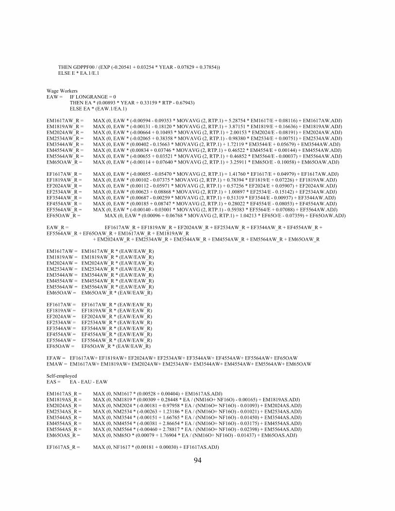
94

THEN GDPPF00 / (EXP (-0.20541 + 0.03254 * YEAR - 0.07829 + 0.37854)) ELSE E * EA.1/E.1 Wage Workers EAW = IF LONGRANGE = 0 THEN EA * (0.00893 * YEAR + 0.33159 * RTP - 0.67943) ELSE EA * (EAW.1/EA.1) EM1617AW_R = MAX (0, EAW * (-0.00594 - 0.09353 * MOVAVG (2, RTP.1) + 5.28754 * EM1617/E + 0.08116) + EM1617AW.ADJ) EM1819AW_R = MAX (0, EAW * (-0.00131 - 0.18120 * MOVAVG (2, RTP.1) + 3.87151 * EM1819/E + 0.16636) + EM1819AW.ADJ) EM2024AW_R = MAX (0, EAW * (-0.00664 + 0.10493 * MOVAVG (2, RTP.1) + 2.00153 * EM2024/E - 0.08191) + EM2024AW.ADJ) EM2534AW_R = MAX (0, EAW * (-0.02065 + 0.38358 * MOVAVG (2, RTP.1) - 0.98380 * EM2534/E + 0.00751) + EM2534AW.ADJ) EM3544AW_R = MAX (0, EAW * (0.00402 - 0.15663 * MOVAVG (2, RTP.1) + 1.72119 * EM3544/E + 0.05679) + EM3544AW.ADJ) EM4554AW_R = MAX (0, EAW * (0.00834 + 0.03746 * MOVAVG (2, RTP.1) + 0.46522 * EM4554/E + 0.00144) + EM4554AW.ADJ) EM5564AW_R = MAX (0, EAW * (-0.00655 + 0.03521 * MOVAVG (2, RTP.1) + 0.46852 * EM5564/E - 0.00037) + EM5564AW.ADJ) EM65OAW_R = MAX (0, EAW * (-0.00114 + 0.07640 * MOVAVG (2, RTP.1) + 3.25911 * EM65O/E - 0.10058) + EM65OAW.ADJ) EF1617AW_R = MAX (0, EAW * (-0.00055 - 0.05470 * MOVAVG (2, RTP.1) + 1.41760 * EF1617/E + 0.04979) + EF1617AW.ADJ) EF1819AW_R = MAX (0, EAW * (0.00102 - 0.07375 * MOVAVG (2, RTP.1) + 0.78394 * EF1819/E + 0.07226) + EF1819AW.ADJ) EF2024AW_R = MAX (0, EAW * (0.00112 - 0.05971 * MOVAVG (2, RTP.1) + 0.57256 * EF2024/E + 0.05907) + EF2024AW.ADJ) EF2534AW_R = MAX (0, EAW * (0.00623 + 0.08868 * MOVAVG (2, RTP.1) + 1.00897 * EF2534/E - 0.15142) + EF2534AW.ADJ) EF3544AW_R = MAX (0, EAW * (0.00687 - 0.00259 * MOVAVG (2, RTP.1) + 0.51319 * EF3544/E - 0.00937) + EF3544AW.ADJ) EF4554AW_R = MAX (0, EAW * (0.00185 + 0.08747 * MOVAVG (2, RTP.1) + 0.28022 * EF4554/E - 0.08053) + EF4554AW.ADJ) EF5564AW_R = MAX (0, EAW * (-0.00140 - 0.03001 * MOVAVG (2, RTP.1) - 0.59383 * EF5564/E + 0.07088) + EF5564AW.ADJ) EF65OAW_R = MAX (0, EAW * (0.00096 + 0.06768 * MOVAVG (2, RTP.1) + 1.04213 * EF65O/E - 0.07359) + EF65OAW.ADJ) EAW_R = EF1617AW_R + EF1819AW_R + EF2024AW_R + EF2534AW_R + EF3544AW_R + EF4554AW_R + EF5564AW_R + EF65OAW_R + EM1617AW_R + EM1819AW_R + EM2024AW_R + EM2534AW_R + EM3544AW_R + EM4554AW_R + EM5564AW_R + EM65OAW_R EM1617AW = EM1617AW_R * (EAW/EAW_R) EM1819AW = EM1819AW_R * (EAW/EAW_R) EM2024AW = EM2024AW_R * (EAW/EAW_R) EM2534AW = EM2534AW_R * (EAW/EAW_R) EM3544AW = EM3544AW_R * (EAW/EAW_R) EM4554AW = EM4554AW_R * (EAW/EAW_R) EM5564AW = EM5564AW_R * (EAW/EAW_R) EM65OAW = EM65OAW_R * (EAW/EAW_R) EF1617AW = EF1617AW_R * (EAW/EAW_R) EF1819AW = EF1819AW_R * (EAW/EAW_R) EF2024AW = EF2024AW_R * (EAW/EAW_R) EF2534AW = EF2534AW_R * (EAW/EAW_R) EF3544AW = EF3544AW_R * (EAW/EAW_R) EF4554AW = EF4554AW_R * (EAW/EAW_R) EF5564AW = EF5564AW_R * (EAW/EAW_R) EF65OAW = EF65OAW_R * (EAW/EAW_R) EFAW = EF1617AW+ EF1819AW+ EF2024AW+ EF2534AW+ EF3544AW+ EF4554AW+ EF5564AW+ EF65OAW EMAW = EM1617AW+ EM1819AW+ EM2024AW+ EM2534AW+ EM3544AW+ EM4554AW+ EM5564AW+ EM65OAW Self-employed EAS = EA - EAU - EAW EM1617AS_R = MAX (0, NM1617 * (0.00528 + 0.00404) + EM1617AS.ADJ) EM1819AS_R = MAX (0, NM1819 * (0.00309 + 0.28448 * EA / (NM16O+ NF16O) - 0.00165) + EM1819AS.ADJ) EM2024AS_R = MAX (0, NM2024 * (-0.00181 + 0.97958 * EA / (NM16O+ NF16O) - 0.01093) + EM2024AS.ADJ) EM2534AS_R = MAX (0, NM2534 * (-0.00263 + 1.23186 * EA / (NM16O+ NF16O) - 0.01021) + EM2534AS.ADJ) EM3544AS_R = MAX (0, NM3544 * (-0.00151 + 1.66765 * EA / (NM16O+ NF16O) - 0.01450) + EM3544AS.ADJ) EM4554AS_R = MAX (0, NM4554 * (-0.00381 + 2.86654 * EA / (NM16O+ NF16O) - 0.03175) + EM4554AS.ADJ) EM5564AS_R = MAX (0, NM5564 * (-0.00460 + 2.78817 * EA / (NM16O+ NF16O) - 0.02398) + EM5564AS.ADJ) EM65OAS_R = MAX (0, NM65O * (0.00079 + 1.76904 * EA / (NM16O+ NF16O) - 0.01437) + EM65OAS.ADJ) EF1617AS_R = MAX (0, NF1617 * (0.00181 + 0.00030) + EF1617AS.ADJ)

95

EF1819AS_R = MAX (0, EM1819AS.1 * (-0.02393 + 0.63672 * MOVAVG (2, RTP.1) + 0.98791 * EF1819/EM1819 - 4.43926) + EF1819AS.ADJ) EF2024AS_R = MAX (0, EM2024AS.1 * (0.07353 - 0.40207 * MOVAVG (2, RTP.1) + 0.57572 * EF2024/EM2024 - 0.01117) + EF2024AS.ADJ) EF2534AS_R = MAX (0, EM2534AS.1 * (0.16575 + 0.16967 * MOVAVG (2, RTP.1) + 0.55503 * EF2534/EM2534 - 0.43412) + EF2534AS.ADJ) EF3544AS_R = MAX (0, EM3544AS.1 * (0.15848 + 0.37839 * MOVAVG (2, RTP.1) + 0.37764 * EF3544/EM3544 - 0.45362) + EF3544AS.ADJ) EF4554AS_R = MAX (0, EM4554AS.1 * (0.21947 + 0.29497 * MOVAVG (2, RTP.1) + 0.58974 * EF4554/EM4554 - 0.51966) + EF4554AS.ADJ) EF5564AS_R = MAX (0, EM5564AS.1 * (0.20892 + 0.36294 * MOVAVG (2, RTP.1) + 0.65320 * EF5564/EM5564 - 0.66626) + EF5564AS.ADJ) EF65OAS_R = MAX (0, EM65OAS.1 * (0.16242 + 0.54916 * MOVAVG (2, RTP.1) + 0.06199 * EF65O/EM65O- 0.47556) + EF65OAS.ADJ) EAS_R = EF1617AS_R + EF1819AS_R + EF2024AS_R + EF2534AS_R + EF3544AS_R + EF4554AS_R + EF5564AS_R + EF65OAS_R + EM1617AS_R + EM1819AS_R + EM2024AS_R + EM2534AS_R + EM3544AS_R + EM4554AS_R + EM5564AS_R + EM65OAS_R EM1617AS = EM1617AS_R * (EAS/EAS_R) EM1819AS = EM1819AS_R * (EAS/EAS_R) EM2024AS = EM2024AS_R * (EAS/EAS_R) EM2534AS = EM2534AS_R * (EAS/EAS_R) EM3544AS = EM3544AS_R * (EAS/EAS_R) EM4554AS = EM4554AS_R * (EAS/EAS_R) EM5564AS = EM5564AS_R * (EAS/EAS_R) EM65OAS = EM65OAS_R * (EAS/EAS_R) EF1617AS = EF1617AS_R * (EAS/EAS_R) EF1819AS = EF1819AS_R * (EAS/EAS_R) EF2024AS = EF2024AS_R * (EAS/EAS_R) EF2534AS = EF2534AS_R * (EAS/EAS_R) EF3544AS = EF3544AS_R * (EAS/EAS_R) EF4554AS = EF4554AS_R * (EAS/EAS_R) EF5564AS = EF5564AS_R * (EAS/EAS_R) EF65OAS = EF65OAS_R * (EAS/EAS_R) EFAS = EF1617AS + EF1819AS + EF2024AS + EF2534AS + EF3544AS + EF4554AS + EF5564AS + EF65OAS EMAS = EM1617AS + EM1819AS + EM2024AS + EM2534AS + EM3544AS + EM4554AS + EM5564AS + EM65OAS Unpaid Family Workers EM1617AU_R = MAX (0, 0.002 + EM1617AU.ADJ) EM1819AU_R = MAX (0, 0.001 + EM1819AU.ADJ) EM2024AU_R = MAX (0, 0.001 + EM2024AU.ADJ) EM2534AU_R = MAX (0, 0.003 + EM2534AU.ADJ) EM3544AU_R = MAX (0, 0.004 + EM3544AU.ADJ) EM4554AU_R = MAX (0, 0.005 + EM4554AU.ADJ) EM5564AU_R = MAX (0, 0.003 + EM5564AU.ADJ) EM65OAU_R = MAX (0, 0.001 + EM65OAU.ADJ) EF1617AU_R = MAX (0, 0.006 + EM1617AU.ADJ) EF1819AU_R = MAX (0, 0.005 + EF1819AU.ADJ) EF2024AU_R = MAX (0, 0.005 + EF2024AU.ADJ) EF2534AU_R = MAX (0, 0.002 + EF2534AU.ADJ) EF3544AU_R = MAX (0, 0.002 + EF3544AU.ADJ) EF4554AU_R = MAX (0, 0.001 + EF4554AU.ADJ) EF5564AU_R = MAX (0, 0.001 + EF5564AU.ADJ) EF65OAU_R = MAX (0, 0.002 + EF65OAU.ADJ) EAU_R = EF1617AU_R + EF1819AU_R + EF2024AU_R + EF2534AU_R + EF3544AU_R + EF4554AU_R + EF5564AU_R + EF65OAU_R + EM1617AU_R + EM1819AU_R + EM2024AU_R + EM2534AU_R + EM3544AU_R + EM4554AU_R + EM5564AU_R + EM65OAU_R

96

EAU = IF LONGRANGE = 0 THEN EAU_R ELSE EAU.1/EA.1 * EA EM1617AU = EM1617AU_R * (EAU/EAU_R) EM1819AU = EM1819AU_R * (EAU/EAU_R) EM2024AU = EM2024AU_R * (EAU/EAU_R) EM2534AU = EM2534AU_R * (EAU/EAU_R) EM3544AU = EM3544AU_R * (EAU/EAU_R) EM4554AU = EM4554AU_R * (EAU/EAU_R) EM5564AU = EM5564AU_R * (EAU/EAU_R) EM65OAU = EM65OAU_R * (EAU/EAU_R) EF1617AU = EF1617AU_R * (EAU/EAU_R) EF1819AU = EF1819AU_R * (EAU/EAU_R) EF2024AU = EF2024AU_R * (EAU/EAU_R) EF2534AU = EF2534AU_R * (EAU/EAU_R) EF3544AU = EF3544AU_R * (EAU/EAU_R) EF4554AU = EF4554AU_R * (EAU/EAU_R) EF5564AU = EF5564AU_R * (EAU/EAU_R) EF65OAU = EF65OAU_R * (EAU/EAU_R) EFAU = EF1617AU + EF1819AU + EF2024AU + EF2534AU + EF3544AU + EF4554AU + EF5564AU + EF65OAU EMAU = EM1617AU + EM1819AU + EM2024AU + EM2534AU + EM3544AU + EM4554AU + EM5564AU + EM65OAU ANNUAL "AVERAGE HOURS WORKED" EQUATIONS Total Nonagricultural sector Wage Workers Males AHWM1617NAW = 34.4953 * RTP + 1.03247 * MINW/CPIW_U - 31.4229 * RNM1617S- 0.12369 * 1 + 12.1981 AHWM1819NAW = 32.4361 * RTP + 12.8742 * RTP.1 + 1.28624 * MINW/CPIW_U- 16.0989 * RNM1819S - 0.27834 * 1 - 8.58664 AHWM2024NAW = 20.1161 * RTP - 10.2292 * RNM2024S - 2.28628 * (PM2024NM * NM2024NM / (PM2024NM * NM2024NM + PM2024MS * NM2024MS + PM2024MA * NM2024MA)) + 23.2252 AHWM2534NAW = 17.0559 * RTP - 0.29076 * 1 + 0.04542 *YEAR + 22.5121 AHWM3544NAW = 18.3314 * RTP - 0.30475 * 1 + 0.04409 *YEAR + 22.3275 AHWM4554NAW = 16.0678 * RTP - 0.12289 * 1 + 0.07446 *YEAR + 21.4366 AHWM5564NAW = 10.8277 * RTP + 0.23715 * 1 + 30.8975 AHWM65ONAW = -0.28038 * 1 + 5.40682 * RTP + 25.4797 Females AHWF1617NAW = 17.2598 * RTP + 7.31262 * RTP.1 - 24.9241 * RNF1617S + 16.9218 AHWF1819NAW = 18.7922 * RTP + 13.1066 * RTP.1 - 18.9417 * RNF1819S- 16.2182 * PF1819 + 0.81920 * 1 + 16.7826 AHWF2024NAW = -219.154 * PF2024 + 12.4226 * RTP - 0.98470 * 1 + 158.354 * (PF2024)2 + 98.6034 AHWF2534NAW = -39.2904 * PF2534 + 39.6515 * (PF2534)2 + 9.10839 * RTP- 0.33503 * 1 + 35.8525 AHWF3544NAW = -39.2904 * PF3544 + 39.6515 * (PF3544)2 + 7.40115 * RTP- 0.38214 * 1 + 36.9133 AHWF4554NAW = 8.64511 * RTP - 63.8042 * PF4554 + 59.9107 * (PF4554)2 - 0.58355 * 1 + 44.0723 AHWF5564NAW = 6.61506 * RTP - 0.28969 * 1 + 8.36882 * PF5564 + 24.8288 AHWF65ONAW = -0.43916 * 1 + 26.5228 + (8.36882/2) * (PF65O- 0.086) Self-employed AHWNAS = 24.9592 * RTP - 17.2194 * EFNAS/ENAS + 22.0120 Unpaid Family Workers AHWNAU = 25.5124 * (EF2534NAU + EF3544NAU + EF4554NAU)/ENAU + 19.2730 Agricultural sector Wage Workers AHWAW = 6.58073 * RTP + 14.9130 * RTP.1 + 19.7800

97

Self-employed AHWAS = 2.45830 * PGDPAF/PGDP - 3.61107 * 1 + 44.5318 Unpaid Family Workers AHWAU = 39.3563 QUARTERLY "AVERAGE HOURS WORKED" EQUATIONS Total AHW = (AHWNA * ENA + AHWA * EA) / E Nonagricultural sector AHWNA = (AHWNAW * (E-ENAS-ENAU-EA) + AHWNAS * ENAS + AHWNAU * ENAU) / ENA Wage Workers AHWNAW = (AHWMNAW * (EM – EMNAS - EMNAU – EMAW - EMAS - EMAU) + AHWFNAW * (EF - EFNAS - EFNAU – EFAW - EFAS – EFAU))/ (E – ENAS – ENAU – EA) Males AHWMNAW1 = AHWM1617NAW * (EM1617 - EM1617NAS - EM1617NAU - EM1617AW - EM1617AS - EM1617AU) AHWMNAW2 = AHWM1819NAW * (EM1819 - EM1819NAS - EM1819NAU - EM1819AW - EM1819AS - EM1819AU) AHWMNAW3 = AHWM2024NAW * (EM2024 - EM2024NAS - EM2024NAU - EM2024AW - EM2024AS - EM2024AU) AHWMNAW4 = AHWM2534NAW * (EM2534 - EM2534NAS - EM2534NAU - EM2534AW - EM2534AS - EM2534AU) AHWMNAW5 = AHWM3544NAW * (EM3544 - EM3544NAS - EM3544NAU - EM3544AW - EM3544AS - EM3544AU) AHWMNAW6 = AHWM4554NAW * (EM4554 - EM4554NAS - EM4554NAU - EM4554AW - EM4554AS - EM4554AU) AHWMNAW7 = AHWM5564NAW * (EM5564 - EM5564NAS - EM5564NAU - EM5564AW - EM5564AS - EM5564AU) AHWMNAW8 = AHWM65ONAW * (EM65O - EM65ONAS - EM65ONAU - EM65OAW - EM65OAS - EM65OAU) AHWMNAW = (AHWMNAW1 + AHWMNAW2 + AHWMNAW3 + AHWMNAW4 + AHWMNAW5 + AHWMNAW6 + AHWMNAW7 + AHWMNAW8) / (EM - EMNAS - EMNAU - EMAW - EMAS - EMAU) AHWM1617NAW = 34.4953 * MOVAVG (2, RTP.1) + 1.03247 * MINW/CPIW_U - 31.4229 * RNM1617S - 0.12369 * 1 + 12.1981 + AHWM1617NAW.ADJ AHWM1819NAW = 32.4361 * MOVAVG (2, RTP.1) + 12.8742 * MOVAVG (2, RTP.5) + 1.28624 * MINW/CPIW_U - 16.0989 * RNM1819S - 0.27834 * 1 - 8.58664 + AHWM1819NAW.ADJ AHWM2024NAW = 20.1161 * MOVAVG (2, RTP.1) - 10.2292 * RNM2024S - 2.28628 * (PM2024NM * NM2024NM/ (PM2024NM * NM2024NM + PM2024MS * NM2024MS + PM2024MA * NM2024MA)) + 23.2252 + AHWM2024NAW.ADJ AHWM2534NAW = MIN (45, 17.0559 * MOVAVG (2, RTP.1) - 0.29076 * 1 + 0.04542 *YEAR + 22.5121) + AHWM2534NAW.ADJ AHWM3544NAW = MIN (45, 18.3314 * MOVAVG (2, RTP.1) - 0.30475 * 1 + 0.04409 *YEAR + 22.3275) + AHWM3544NAW.ADJ AHWM4554NAW = MIN (45, 16.0678 * MOVAVG (2, RTP.1) - 0.12289 * 1 + 0.07446 *YEAR + 21.4366) + AHWM4554NAW.ADJ AHWM5564NAW = 10.8277 * MOVAVG (2, RTP.1) + 0.23715 * 1 + 30.8975 + AHWM5564NAW.ADJ AHWM65ONAW = -0.28038 * 1 + 5.40682 * MOVAVG (2, RTP.1) + 25.4797 + AHWM65ONAW.ADJ Females AHWFNAW1 = AHWF1617NAW* (EF1617 -EF1617NAS-EF1617NAU-EF1617AW-EF1617AS-EF1617AU) AHWFNAW2 = AHWF1819NAW* (EF1819 -EF1819NAS-EF1819NAU-EF1819AW-EF1819AS-EF1819AU) AHWFNAW3 = AHWF2024NAW* (EF2024 -EF2024NAS-EF2024NAU-EF2024AW-EF2024AS-EF2024AU) AHWFNAW4 = AHWF2534NAW* (EF2534 -EF2534NAS-EF2534NAU-EF2534AW-EF2534AS-EF2534AU) AHWFNAW5 = AHWF3544NAW* (EF3544 -EF3544NAS-EF3544NAU-EF3544AW-EF3544AS-EF3544AU) AHWFNAW6 = AHWF4554NAW* (EF4554 -EF4554NAS-EF4554NAU-EF4554AW-EF4554AS-EF4554AU) AHWFNAW7 = AHWF5564NAW* (EF5564 -EF5564NAS-EF5564NAU-EF5564AW-EF5564AS-EF5564AU) AHWFNAW8 = AHWF65ONAW * (EF65O -EF65ONAS-EF65ONAU-EF65OAW-EF65OAS-EF65OAU) AHWFNAW = (AHWFNAW1 + AHWFNAW2 + AHWFNAW3 + AHWFNAW4 + AHWFNAW5 + AHWFNAW6 + AHWFNAW7 + AHWFNAW8) / (EF – EFAS – EFAU) AHWF1617NAW = 17.2598 * MOVAVG (2, RTP.1) + 7.31262 * MOVAVG (2, RTP.5) - 24.9241 * RNF1617S + 16.9218 + AHWF1617NAW.ADJ

98

AHWF1819NAW = 18.7922 * MOVAVG (2, RTP.1) + 13.1066 * MOVAVG (2, RTP.5) - 18.9417 * RNF1819S - 16.2182 * PF1819 + 0.81920 * 1 + 16.7826 + AHWF1819NAW.ADJ AHWF2024NAW = -219.154 * PF2024 + 12.4226 * MOVAVG (2, RTP.1) - 0.98470 * 1 + 158.354 * (PF2024)2 + 98.6034 + AHWF2024NAW.ADJ AHWF2534NAW = -39.2904 * PF2534 + 39.6515 * (PF2534)2 + 9.10839 * MOVAVG (2, RTP.1) - 0.33503 * 1 + 35.8525 + AHWF2534NAW.ADJ AHWF3544NAW = -39.2904 * PF3544 + 39.6515 * (PF3544)2 + 7.40115 * MOVAVG (2, RTP.1) - 0.38214 * 1 + 36.9133 + AHWF3544NAW.ADJ AHWF4554NAW = 8.64511 * MOVAVG (2, RTP.1) - 63.8042 * PF4554 + 59.9107 * (PF4554)2 - 0.58355 * 1 + 44.0723 + AHWF4554NAW.ADJ AHWF5564NAW = 6.61506 * MOVAVG (2, RTP.1) - 0.28969 * 1 + 8.36882 * PF5564 + 24.8288 + AHWF5564NAW.ADJ AHWF65ONAW = -0.43916 * 1 + 26.5228 + (8.36882/2) * (PF65O- 0.086) + AHWF65ONAW.ADJ Self-employed AHWNAS = 24.9592 * MOVAVG (2, RTP.1) - 17.2194 * EFNAS/ENAS + 22.0120 + AHWNAS.ADJ Unpaid Family Workers AHWNAU = 25.5124 * (EF2534NAU + EF3544NAU + EF4554NAU)/ ENAU + 19.2730 + AHWNAU.ADJ Agricultural sector AHWA = (AHWAW * EAW + AHWAS * EAS + AHWAU * EAU) / EA Wage Workers AHWAW = 6.58073 * MOVAVG (2, RTP.1) + 14.9130 * MOVAVG (2, RTP.5) + 19.7800 + AHWAW.ADJ Self-employed AHWAS = 2.45830 * PGDPAF/PGDP - 3.61107 * 1 + 44.5318 + AHWAS.ADJ Unpaid Family Workers AHWAU = 39.3563 + AHWAU.ADJ OTHER EMPLOYMENT MEASURES Federal Civilian Government and Government Enterprises EGFC = IF LONGRANGE = 0 THEN (EGFC.1 * 1.00940.25) ELSE (EGFC.1 * (E_FE/E_FE.1)) EGEFCPS = IF LONGRANGE = 0 THEN (EGEFCPS.1 * 1.00750.25) ELSE (EGEFCPS.1 * (E_FE/E_FE.1)) EGGEFC = EGFC + EGEFCPS State and Local Government and Government Enterprises EGGESL = IF LONGRANGE = 0 THEN EGGESL.1 * (LC_FE/LC_FE.4)0.25 ELSE EGGESL.1 * (E_FE/E_FE.1) Other Employment Measures DNEDMIL = IF (EDMIL-EDMIL.4) < 0 THEN (EDMIL-EDMIL.4) ELSE 0 EP = E-EGGESL - EGGEFC – EAS - ENAS Compensation and Output Sectors Price Deflator for Medical Services CPIWMS = CPIWMS.1 * (1 + ((CPIW_U/CPIW_U.4)0.25 - 1) * CPIWMSWT) UI and WC Effective Tax Rates TMAXUI_SL = TMAXUI_SL.1 *AWSUI.1/AWSUI.2

99

RELMAX_UI = TMAXUI_SL/AWSUI.1/1000 CR_UI = 0.775 TRATIO_UI = 0.96996 * RELMAX_UI-0.13744 * MOVAVG (4, RTP.1) + 0.10368 * MOVAVG (4, RTP.5) + 0.04887 TRATE_UI = 0.00143 * MOVAVG (4, RU.5) + 0.00128 * MOVAVG (4, RU.9) + 0.00057 * MOVAVG (4, RU.13) + 0.00356 RUIWS1 = CR_UI * TRATIO_UI * TRATE_UI RUIWS2 = 0.32476 * MOVAVG (4, RUIWS1.8 * (WSP.8 -WSPRRB.8 +WSGGESL.8)) / (WSP.1 -WSPRR2.1 +WSGGESL.1) Workers' Compensation RWCWS = RWCWS.1 - (RWCWS.1 - 0.0144)/12 State and Local Government and Government Enterprises TAXMAX = IF QTR = 1 THEN 300.* ROUND (MOVAVG (4, AWSE.5)/MOVAVG (4, AWSE.9) * 1000.* TAXMAX.1/300 +0.5)/1000 ELSE TAXMAX.1 Wages AWSPL = MOVAVG (8, AWSP.1) AWSSPL = MOVAVG (8, AWSSP.1) AWSGGESL = IF LONGRANGE = 0 THEN AWSGGESL.1 * AWSPL/AWSPL.1 ELSE AWSGGESL.1 * AVG_GDP/AVG_GDP.1 * (1 + WS_TO_WSS_D/100)0.25 WSGGESL = AWSGGESL * EGGESL Employer Contribution for Government Social Insurance OASDISL_L = (EMPTROASI + EMPTRDI) * 0.978 * CSLA * WSGGESL HISL_L = EMPTRHI * 1.0 * CSLHI * WSGGESL SOC_UISL = (-0.02821 * MOVAVG (4, RTP.2) + 0.03145) * WSGGESL RSOCSL_WC = RSOCSL_WC.1 - (RSOCSL_WC.1 - 0.176)/12 SOC_WCSL = RSOCSL_WC * RWCWS * WSGGESL SOC_SL = (OASDISL_L + HISL_L + SOC_UISL + SOC_WCSL) Employer Contributions for Employee Pension and Insurance funds Workers' Compensation - employees and annuitants OLI_WCSL = (1 - RSOCSL_WC) * RWCWS * WSGGESL Pensions OLI_RETSL = WSGGESL * (OLI_RETSL.1/WSGGESL.1) Life Insurance - employees and annuitants OLI_GLI_SL = 2.0 * EGGESL * ((WSGGESL/EGGESL) +2.0) * 0.075 * 26/1000 Health Insurance - employees and annuitants OLI_GHI_SL = (OLI_GHI_SL.1 / EGGESL.1) * CPIWMS/CPIWMS.1 * EGGESL * RGR_GHI Total OLI_SL = (OLI_GLI_SL + OLI_GHI_SL + OLI_WCSL + OLI_RETSL) RCWSSL = (1 + (SOC_SL + OLI_SL)/WSGGESL) WSSGGESL = IF LONGRANGE = 0 THEN RCWSSL*WSGGESL ELSE (WSSGGESL.1/EGGESL.1) * AVG_GDP/AVG_GDP.1 * EGGESL WSSGSL = WSSGGESL * WSSGSL.1/WSSGGESL.1 WSSGESL = WSSGGESL - WSSGSL CFCGSL = IF LONGRANGE = 0 THEN WSSGSL * RCFCGSL ELSE CFCGSL.1 * WSSGGESL/WSSGGESL.1 GDPGSL = WSSGSL + CFCGSL CFCGESL = IF LONGRANGE = 0 THEN WSSGESL * RCFCGESL ELSE CFCGESL.1 * WSSGGESL/WSSGGESL.1

100

GDPGESL = WSSGESL + CFCGESL GDPGGESL = GDPGSL + GDPGESL Federal Civilian General Government and Government Enterprises Wages General Government and Government Enterprises CRAZ1 = IF LONGRANGE = 0 THEN ((IF QTR = 1 THEN (0.82429 * (AWSP.6/AWSP.10 - 1) -0.005) ELSE 0)) ELSE (IF QTR = 1 THEN (AWSP.6/AWSP.10 - 1) ELSE 0) MRAZ = IF LONGRANGE = 0 THEN ((IF QTR = 1 THEN (0.82429 * (AWSP.6/AWSP.10 - 1) -0.005) ELSE 0)) ELSE (IF QTR = 1 THEN (AWSP.6/AWSP.10 - 1) ELSE 0) AWSGGEFC = IF LONGRANGE = 0 THEN (AWSGGEFC.1 * (1 +1.0 *CRAZ1 +0.0015)) ELSE AWSGGEFC.1 * AVG_GDP/AVG_GDP.1 * (1 +WS_TO_WSS_D/100)0.25 WSGGEFC = AWSGGEFC * EGGEFC CSRS workers AWEFC_N = IF LONGRANGE = 0 THEN (AWEFC_N.1 * (1 +1.0 *CRAZ1 +0.00082)) ELSE AWEFC_N.1 * AVG_GDP/AVG_GDP.1 * (1 +WS_TO_WSS_D/100)0.25 WEFC_N = AWEFC_N * TEFC_N Government Enterprises (Mostly U.S. Postal Service) AWSGEFC = IF LONGRANGE = 0 THEN (AWSGEFC.1 * (1 +1.0 *CRAZ1 +0.0015)) ELSE AWSGEFC.1 * AVG_GDP/AVG_GDP.1 * (1 +WS_TO_WSS_D/100) 0.25 WSGEFC = AWSGEFC * EGEFCPS General Government WSGFC = WSGGEFC -WSGEFC AWSGFC = WSGFC/EGFC Employer Contribution for Government Social Insurance General Government and Government Enterprises OASDIFC_L = (EMPTROASI + EMPTRDI) * 1.04 * (WSGGEFC - WEFC_N) * ADJ_FSA_FC HIFC_L = EMPTRHI* 1.055 * WSGGEFC * ADJ_FSA_FC SOCF_UIFC = (-0.05934 * RTP + 0.06165) * WSGGEFC SOCF_WC = 0.0159 * WSGGEFC SOC_FC = (SOCF_UIFC + SOCF_WC + OASDIFC_L + HIFC_L) Employer Contributions for Employee Pension and Insurance funds General Government and Government Enterprises Pensions OLI_CSRS1 = ((0.174 * WSGEFC + 0.07 * WSGFC) / WSGGEFC) * WEFC_N OLI_FERS1 = 0.107 * (WSGGEFC * 0.9 -WEFC_N) OLI_FERSFC = 0.048 * (WSGGEFC * 0.9 -WEFC_N) OLI_RETFC = OLI_CSRS1 + OLI_FERS1 + OLI_FERSFC + OLIF_RETFCO Life Insurance - employees and annuitants OLI_GLI_FC = 2.0 * EGGEFC * ((WSGGEFC/EGGEFC) + 2.0) * 0.075 * 26/1000

101

Health Insurance - employees and annuitants OLI_GHI_FC = (OLI_GHI_FC.1 / EGGEFC.1) * CPIWMS/CPIWMS.1 * EGGEFC * RGR_GHI OLI_FC = (OLI_GHI_FC + OLI_GLI_FC + OLI_RETFC) Compensation General Government and Government Enterprises RCWSF = (1 + (SOC_FC + OLI_FC)/WSGGEFC) WSSGGEFC = IF LONGRANGE = 0 THEN RCWSF * WSGGEFC ELSE (WSSGGEFC.1/EGGEFC.1) * AVG_GDP/AVG_GDP.1 * EGGEFC WSSGFC = IF LONGRANGE = 0 THEN RCWSF * WSGFC ELSE (WSSGFC.1 / (EGGEFC.1 - EGEFCPS.1)) * AVG_GDP/AVG_GDP.1 * (EGGEFC - EGEFCPS) WSSGEFC = IF LONGRANGE = 0 THEN RCWSF * WSGEFC ELSE (WSSGEFC.1/EGEFCPS.1) * AVG_GDP/AVG_GDP.1 * EGEFCPS Consumption of Fixed Capital General Government and Government Enterprises CFCGFC = IF LONGRANGE = 0 THEN WSSGFC * RCFCGFC ELSE CFCGFC.1 * WSSGGEFC / WSSGGEFC.1 CFCGEFC = IF LONGRANGE = 0 THEN WSSGEFC * RCFCGEFC ELSE CFCGEFC.1 * WSSGGEFC / WSSGGEFC.1 Gross Domestic Product General Government and Government Enterprises GDPGFC = WSSGFC + CFCGFC GDPGEFC = WSSGEFC + CFCGEFC GDPGGEFC = GDPGFC + GDPGEFC Federal Government Military Wages AWSGFM = IF LONGRANGE = 0 THEN (AWSGFM.1 * (1.0027 +1.0 * MRAZ)) ELSE AWSGFM.1 * AVG_GDP/AVG_GDP.1 * (1 + WS_TO_WSS_D/100) 0.25 WSGFM = AWSGFM * (EDMIL+ EDMIL_R) Employer Contribution for Government Social Insurance OASDIFM_L = (EMPTROASI + EMPTRDI) * 0.9975 * CML * WSGFM HIFM_L = EMPTRHI* 1.0 *CML * WSGFM SOCF_UIFM = MAX (0.001, (-0.05263 * DIFF (EDMIL + EDMIL_R) - 0.03079 * RTP + 0.03310)) * WSGFM SOCF_MIFM = 0.30 * CPIWMS * (EDMIL + EDMIL_R) SOC_FM = (SOCF_UIFM + SOCF_MIFM + OASDIFM_L + HIFM_L) Employer Contributions for Employee Pension and Insurance funds OLI_RETFM = (OLI_RETFM.1/WSGFM.1 - (OLI_RETFM.1/WSGFM.1 - 0.472)/12) * WSGFM Compensation RCWSM = (1 + (OLI_RETFM + SOC_FM)/WSGFM) WSSGFM = IF LONGRANGE = 0 THEN RCWSM * WSGFM ELSE (WSSGFM.1/EDMIL.1) * AVG_GDP/AVG_GDP.1 * EDMIL

102

Consumption of Fixed Capital CFCGFM = IF LONGRANGE = 0 THEN WSSGFM * RCFCGFM ELSE CFCGFM.1 * WSSGFM/WSSGFM.1 Gross Domestic Product GDPGFM = WSSGFM + CFCGFM GDPGF = GDPGFC + GDPGFM GDPGGE = GDPGGEFC + GDPGGESL + GDPGFM Total (Civilian and Military) Federal General Government and Government Enterprises WSSGF = WSSGFC + WSSGFM WSSGE = WSSGEFC + WSSGESL WSSG = WSSGF + WSSGSL GDPGE = GDPGEFC + GDPGESL GDPG = GDPGF + GDPGSL NIPA Farm Output and Earnings GDPPF00 = IF LONGRANGE = 0 THEN EXP (- 3.52340 + 0.02055 * YEAR) * N_SSA ELSE GDPPF00.1 * GDP00/GDP00.1 PGDPAF = IF LONGRANGE = 0 THEN PGDPAF.1 * ((PGDP/PGDP.1)4 - 0.01) 0.25 ELSE PGDPAF.1 * ((PGDP/PGDP.1)4) 0.25 GDPPF = GDPPF00 * PGDPAF AYF_K = ((YF.1 /EAS.1) / (WSSPF.1/EAW.1) - 1.594) * 0.8 + 1.594 WSSPF = IF LONGRANGE = 0 THEN EAW * MOVAVG (4, WSSP.2/EP.2) * (3.15749 / (YEAR- 65) - 0.43419 * RTP + 0.68725) ELSE (WSSPF.1/EAW.1) * AVG_GDP/AVG_GDP.1 * EAW WSPF = IF LONGRANGE = 0 THEN WSSPF * (MOVAVG (12, (WSP.1/WSSP.1)) + 0.015) ELSE (WSPF.1 /WSSPF.1) * (WSP.1/WSSP.1) / (WSP.2/WSSP.2) * WSSPF AWSPF = WSPF/EAW YF = AYF_K * (WSSPF/EAW) * EAS GDP, WSS and WS, Private Households & Nonprofit Institutions Private Households Compensation & Wages WSSPH = IF LONGRANGE = 0 THEN (((WSSPH.1/ENAWPH.1)/MOVAVG (4, WSSP.3/EP.3) - 0.41) * 0.875 + 0.41) * MOVAVG (4, WSSP.2/EP.2) * ENAWPH ELSE (AVG_GDP/AVG_GDP.1) * ENAWPH * (WSSPH.1/ENAWPH.1) WSPH = IF LONGRANGE = 0 THEN WSSPH / (1 +CPH* 1 * (EMPTROASI + EMPTRDI + EMPTRHI)) ELSE (AWSPH.1 * ENAWPH.1/WSSPH.1) * (1 + WS_TO_WSS_D/100) 0.25 * WSSPH AWSPH = WSPH / ENAWPH Owner Occupied Housing OOH = OOH.1 * (KGDP00 * PGDP) / (KGDP00.1 * PGDP.1) Gross Value Added GDPPH = IF LONGRANGE = 0 THEN WSSPH + OOH ELSE (AVG_GDP/AVG_GDP.1) * ENAWPH * (GDPPH.1/ENAWPH.1)

103

Nonprofit Institutions Health Services EPHS_EST = IF LONGRANGE = 0 THEN EPHS_EST.1 + 0.275/4 ELSE EPHS_EST.1 * (E_FE/E_FE.1) AWSSPHS = IF LONGRANGE = 0 THEN AWSSPHS.1 * AWSSPL/AWSSPL.1 ELSE AWSSPHS.1 * AVG_GDP/AVG_GDP.1 WSSPHS = AWSSPHS* EPHS_EST Educational Services EPES_EST = IF LONGRANGE = 0 THEN EPES_EST.1 + 0.075/4 ELSE EPES_EST.1 * (E_FE/E_FE.1) AWSSPES = IF LONGRANGE = 0 THEN AWSSPES.1 * AWSSPL/AWSSPL.1 ELSE AWSSPES.1 * AVG_GDP/AVG_GDP.1 WSSPES = AWSSPES* EPES_EST Social Services EPSS_EST = IF LONGRANGE = 0 THEN EPSS_EST.1 + 0.075/4 ELSE EPSS_EST.1 * (E_FE/E_FE.1) AWSSPSS = IF LONGRANGE = 0 THEN AWSSPSS.1 * AWSSPL/AWSSPL.1 ELSE AWSSPSS.1 * AVG_GDP/AVG_GDP.1 WSSPSS = AWSSPSS* EPSS_EST Gross Value Added WSSPNI = WSSPNI.1 * (WSSPHS + WSSPES + WSSPSS) / (WSSPHS.1 + WSSPES.1 + WSSPSS.1) WSPNI = IF LONGRANGE = 0 THEN WSSPNI * (WSPNI.1/WSSPNI.1) * ((WSP.1/WSSP.1) / (WSP.9/WSSP.9)) (1/8) ELSE WSSPNI * (WSPNI.1/WSSPNI.1) * (1 +WS_TO_WSS_D/100) 0.25 GDPPNI = IF LONGRANGE = 0 THEN WSSPNI / ((WSSPNI.1/GDPPNI.1 - 0.866) * 0.8 + 0.866) ELSE WSSPNI /0.866 Private Output and Compensation SOC ROASDIP_L = (EMPTROASI + EMPTRDI) * TXRP * CP RHIP_L = EMPTRHI * 1.0 * CP RSOC_UIP = 0.00109 * MOVAVG (4, RU.2) + 0.00045 * MOVAVG (4, RU.10) + 0.00048 * MOVAVG (4, RU.18) - 0.00331 RSOC_WCP = RWCWS * RSOCSL_WC RSOCF_PBG = 0.00022 OLI ROLI_WCP = RWCWS * (1 - RSOCSL_WC) ROLI_SU = 0.0005 OLI_GLI_P = 0.0025 * EP * AWSP.1 OLI_GHI_P = (OLI_GHI_P.1 / EP.1) * CPIWMS/CPIWMS.1 * EP * RGR_GHI ROLI_PPPS = MAX (ROLI_PPPS.1, 0.00031 * YEAR + 0.00866) WSS and YNF WSSGGE = (WSSGGESL + WSSGGEFC + WSSGFM) GDPPBNFXGE = (GDP – GDPGGE – GDPPF – GDPPH – GDPPNI) RWSSPBNFXGE = (-0.35334 * DRTPP - 0.16925 * DRTPP.1 + 0.20074 * DRTPN.1 + 0.16114 * DRTPN.2 + 0.59442) ENAW = ENA-ENAS-ENAU

104

ENAWPBXGE = ENAW - (ENAWPH + EGGEFC + EGGESL + WSSPNI / (WSSPHS + WSSPES + WSSPSS) * (EPHS_EST + EPES_EST + EPSS_EST)) ENAWSPBXGE = ENAWPBXGE + ENAS AYNF_K = ((YNF.1/ENAS.1 / (WSSPBNFXGE.1/ENAWPBXGE.1)) - 1.65) * 0.9 + 1.65 AYF = YF/EAS AWSSPF = WSSPF/EAW AYNF = YNF/ENAS AWSSPBNFXGE = WSSPBNFXGE/ENAWPBXGE YNF = YNF.1 * (GDPPBNFXGE / GDPPBNFXGE.1) * (ENAS / (ENAS + ENAWPBXGE)) / (ENAS.1 / (ENAS.1 + ENAWPBXGE.1)) WSSPBNFXGE = (GDPPBNFXGE - YNF) * ((WSSPBNFXGE.1 / (GDPPBNFXGE.1 - YNF.1) - 0.621) * (0.8) + 0.621) WSSP = WSSPBNFXGE+WSSPF+WSSPH +WSSPNI RCWSP = WSSP / (WSSP - SOCF_RETRR - OLI_GLI_P - OLI_GHI_P) * (1 + ROASDIP_L + RHIP_L + RSOC_UIP + RSOC_WCP + RSOCF_PBG + ROLI_WCP + ROLI_SU + ROLI_PPPS) WS = IF WS_TO_WSS_DYR = 0 THEN (WSGGESL + WSGGEFC + WSGFM + WSSP/RCWSP) ELSE WSS * WS.1/WSS.1 * (1 + WS_TO_WSS_D/100) 0.25 WSP = (WS - WSGGESL - WSGGEFC - WSGFM) AWSP = WSP/EP AWSSP = WSSP/EP Other Variables WSD = WS WSDP = (WSD –WSGGESL – WSGGEFC – WSGFM) AWSE = WS / (E + EDMIL – EAS – ENAS) AWSUI = (WS -WSGGEFC -WSGFM) / (E – EGGEFC – EAS – ENAS) WSS = (WSSP + WSSGGE) OLI = OLI_GGE + OLI_P SOC = SOC_GGE + SOC_P OLI_GGE = OLI_FC + OLI_SL + OLI_RETFM SOC_GGE = SOC_FC + SOC_FM + SOC_SL SOC_UIP = RSOC_UIP * WSP SOC_WCP = RSOC_WCP * WSP OASDIP_L = ROASDIP_L * WSP HIP_L = RHIP_L * WSP SOCF_PBG = RSOCF_PBG * WSP SOCF_RETRR = 0.20 * WSPRRB SOC_P = SOC_UIP + SOC_WCP + OASDIP_L + HIP_L + SOCF_PBG + SOCF_RETRR OLI_WCP = ROLI_WCP * WSP OLI_SU = ROLI_SU * WSP OLI_PPPS = ROLI_PPPS * WSP OLI_P = OLI_WCP + OLI_SU + OLI_GHI_P + OLI_GLI_P + OLI_PPPS OLI_PPS = OLI_PPPS + OLI_RETFC + OLI_RETFM + OLI_RETSL OLI_GHI = OLI_GHI_P + OLI_GHI_FC + OLI_GHI_SL OLI_GLI = OLI_GLI_P + OLI_GLI_FC + OLI_GLI_SL OLI_WC = OLI_WCP + OLI_WCSL SOCSL_WC = SOC_WCSL + SOC_WCP SOCF_UIFED = SOCF_UIFC + SOCF_UIFM SOCF_UIS = (SOC_UIP + SOC_UISL) * RUIWS1 / (RUIWS1 + RUIWS2) SOCF_UIF = (SOC_UIP + SOC_UISL) - SOCF_UIS SOCF_OASDI = OASDIP_L + OASDISL_L + OASDIFC_L + OASDIFM_L SOCF_HI = HIP_L + HISL_L + HIFC_L + HIFM_L

105

2.3 OASDI Covered Employment and Earnings (COV) Total At-Any-Time Employment Males Aged 1 through 9 CEM1 = 0.00026 * NM1 CEM2 = 0.00031 * NM2 CEM3 = 0.00025 * NM3 CEM4 = 0.00019 * NM4 CEM5 = 0.00036 * NM5 CEM6 = 0.00042 * NM6 CEM7 = 0.00165 * NM7 CEM8 = 0.00239 * NM8 CEM9 = 0.00279 * NM9 Aged 10 through 15 TEM1013 = 0.01969 * (NM10 + NM11 + NM12 + NM13 + NM10[+1] + NM11[+1] + NM12[+1] + NM13[+1])/2 TEM1415 = (0.42767 * RTP - 1.02624 * NM1415 / (NM1415 + NM1617) + 0.23102) * ((NM14 + NM15 + NM14[+1] + NM15[+1])/2) Females Aged 1 through 9 CEF1 = 0.00028 * NF1 CEF2 = 0.00023 * NF2 CEF3 = 0.00020 * NF3 CEF4 = 0.00031 * NF4 CEF5 = 0.00041 * NF5 CEF6 = 0.00055 * NF6 CEF7 = 0.00129 * NF7 CEF8 = 0.00156 * NF8 CEF9 = 0.00212 * NF9 Aged 10 through 15 TEF1013 = IF YEAR < = 110 THEN (0.04615 * RTP - 0.00014 * YEAR - 0.02268) * (NF10 + NF11 + NF12 + NF13 + NF10[+1] + NF11[+1] + NF12[+1] + NF13[+1])/2 ELSE (0.04615 * RTP - 0.00014 * 110 - 0.02268) * (NF10 + NF11 + NF12 + NF13 + NF10[+1] + NF11[+1] + NF12[+1] + NF13[+1])/2 TEF1415 = (0.48500 * RTP - 0.79002 * NF1415 / (NF1415 + NF1617) + 0.02205) * ((NF14 + NF15 + NF14[+1] + NF15[+1])/2) Total Males, Total Females and Combined Total TEM = CEM1 + CEM2 + CEM3 + CEM4 + CEM5 + CEM6 + CEM7 + CEM8 + CEM9 + TEM1013 + TEM1415 + TEM16O TEF = CEF1 + CEF2 + CEF3 + CEF4 + CEF5 + CEF6 + CEF7 + CEF8 + CEF9 + TEF1013 + TEF1415 + TEF16O TE = TEM + TEF Male Disaggregates Aged 16 and Over TEM1617 = (-0.0337 - 1.32778 * REM1617_A + 1.11118 + RNM1617MAX-0.5 * 0.0637 - 0.161 * RILEM1519) * (EM1617 * REM1617_M * REM2_1617 - EM1617AU - EM1617NAU + NM1617M) TEM1819 = (-0.0267 - 0.60094 * REM1819_A + 0.89703 + RNM1819MAX-0.5 * 0.0637 - 0.265 * RILEM1519) * (EM1819 * REM1819_M * REM2_1819 - EM1819AU- EM1819NAU + NM1819M) TEM2024 = (-0.0196 + 0.02072 + 0.82020 + RNM2024MAX-0.50 * 0.0176 - 0.357 * RILEM2024 -0.80 * (REM2024_A + RM2024D)) * (EM2024 * REM2024_M * REM2_2024 - EM2024AU - EM2024NAU + NM2024M) TEM2529 = (-0.0113 + 0.02898 + 0.81312 + RNM2529MAX-0.50 * 0.0214 - 0.416 * RILEM2529 - 0.80 * (REM2529_A + RM2529D)) * (EM2529 * REM2529_M * REM2_2529 - EM2529AU - EM2529NAU + NM2529M) TEM3034 = (0.0062 - 0.00445 + 0.55577 + RNM3034MAX-0.50 * 0.0416 - 0.424 * RILEM3034 - 0.50 * (REM3034_A + RM3034D)) * (EM3034 * REM3034_M * REM2_3034 - EM3034AU - EM3034NAU + NM3034M) TEM3539 = (-0.0092 + 0.00162 + 0.50480 + RNM3539MAX-0.50 * 0.0279 - 0.423 * RILEM3539 -0.45 * (REM3539_A + RM3539D)) * (EM3539 * REM3539_M * REM2_3539 - EM3539AU - EM3539NAU + NM3539M) TEM4044 = (-0.0083 + 0.01717 + 0.41973 + RNM4044MAX-0.50 * 0.0062 - 0.418 * RILEM4044 - 0.40 * (REM4044_A + RM4044D)) * (EM4044 * REM4044_M * REM2_4044 - EM4044AU - EM4044NAU + NM4044M)

106

TEM4549 = (-0.0026 - 0.00292 + 0.52707 + RNM4549MAX-0.50 * 0.0010 - 0.410 * RILEM4549 -0.50 * (REM4549_A + RM4549D)) * (EM4549 * REM4549_M * REM2_4549 - EM4549AU-EM4549NAU + NM4549M) TEM5054 = (-0.0008 + 0.02301 + 0.53226 + RNM5054MAX - 0.50 * 0.0025 - 0.395 * RILEM5054 -0.50 * (REM5054_A + RM5054D)) * (EM5054 * REM5054_M * REM2_5054 -EM5054AU-EM5054NAU + NM5054M) TEM5559 = (-0.0010 - 0.00842 + 0.46888 + RNM5559MAX - 0.50 * 0.0042 - 0.356 * RILEM5559 -0.40 * (REM5559_A + RM5559D)) * (EM5559 * REM5559_M * REM2_5559 -EM5559AU-EM5559NAU + NM5559M) TEM6064 = (-0.0030 + 0.04966 + 0.59056 + RNM6064MAX - 0.50 * 0.0051 - 0.248 * RILEM6064 - 0.50 * (REM6064_A + RM6064D)) * (EM6064 * REM6064_M * REM2_6064 -EM6064AU-EM6064NAU) TEM6569 = (-0.82949 * REM6569_A + 0.10116 + 1.55172) * (EM6569 * REM6569_M * REM2_6569 - EM6569AU - EM6569NAU) TEM70O = (0.01973 * 96 - 0.34903) * (EM70O* REM70O_M * REM2_70O-EM70OAU-EM70ONAU) TEM16O = TEM1617 + TEM1819 + TEM2024 + TEM2529 + TEM3034 + TEM3539 + TEM4044 + TEM4549 + TEM5054 + TEM5559 + TEM6064 + TEM6569 + TEM70O Female Disaggregates Aged 16 and Over TEF1617 = (0.0106 - 1.52661 * REF1617_A - 0.02280 + 1.17229 + RNF1617MAX + 0.5 * 0.0631 - 0.161 * RILEF1519) * (EF1617 * REF1617_M * REF2_1617 - EF1617AU - EF1617NAU + NF1617M) TEF1819 = (0.0166 - 0.56521 * REF1819_A + 0.04837 + 0.85527 + RNF1819MAX-0.5 * 0.0631 - 0.252 * RILEF1519) * (EF1819 * REF1819_M * REF2_1819 - EF1819AU - EF1819NAU + NF1819M) TEF2024 = (0.0202 + 0.02418 + 0.89686 + RNF2024MAX - 0.50 * 0.0349 - 0.318 * RILEF2024 - 0.90 * (REF2024_A + RF2024D)) * (EF2024 * REF2024_M * REF2_2024 - EF2024AU - EF2024NAU + NF2024M) TEF2529 = (0.0185 + 0.03554 + 0.68431 + RNF2529MAX - 0.50 * 0.0378 - 0.342 * RILEF2529 - 0.70 * (REF2529_A + RF2529D)) * (EF2529 * REF2529_M * REF2_2529 - EF2529AU - EF2529NAU + NF2529M) TEF3034 = (0.0156 + 0.00488 + 0.47083 + RNF3034MAX - 0.50 * 0.0465 - 0.340 * RILEF3034 - 0.45 * (REF3034_A + RF3034D)) * (EF3034 * REF3034_M * REF2_3034 - EF3034AU - EF3034NAU + NF3034M) TEF3539 = (0.0156 + 0.000796 + 0.41423 + RNF3539MAX - 0.50 * 0.0318 - 0.343 * RILEF3539 - 0.40 * (REF3539_A + RF3539D)) * (EF3539 * REF3539_M * REF2_3539 - EF3539AU - EF3539NAU + NF3539M) TEF4044 = (0.0127 + 0.00312 + 0.35298 + RNF4044MAX - 0.50 * 0.0135 - 0.353 * RILEF4044 - 0.35 * (REF4044_A + RF4044D)) * (EF4044 * REF4044_M * REF2_4044 - EF4044AU - EF4044NAU + NF4044M) TEF4549 = (0.0064 + 0.00138 + 0.40080 + RNF4549MAX - 0.50 * 0.0086 - 0.358 * RILEF4549 - 0.40 * (REF4549_A + RF4549D)) * (EF4549 * REF4549_M * REF2_4549 - EF4549AU - EF4549NAU + NF4549M) TEF5054 = (0.0037 + 0.01202 + 0.39021 + RNF5054MAX - 0.50 * 0.0089 - 0.336 * RILEF5054 - 0.40 * (REF5054_A + RF5054D)) * (EF5054 * REF5054_M * REF2_5054 - EF5054AU - EF5054NAU + NF5054M) TEF5559 = (0.0034 + 0.03036 + 0.32074 + RNF5559MAX - 0.50 * 0.0094 - 0.280 * RILEF5559 - 0.30 * (REF5559_A + RF5559D)) * (EF5559 * REF5559_M * REF2_5559 - EF5559AU - EF5559NAU + NF5559M) TEF6064 = (0.0030 + 0.02068 + 0.49318 + RNF6064MAX - 0.50 * 0.0115 - 0.176 * RILEF6064 - 0.45 * (REF6064_A + RF6064D)) * (EF6064 * REF6064_M * REF2_6064 - EF6064AU - EF6064NAU) TEF6569 = 1.42 * (EF6569 * REF6569_M * REF2_6569 - EF6569AU - EF6569NAU) TEF70O = (0.92002 * TEM70O / (EM70O* REM70O_M * REM2_70O - EM70OAU - EM70ONAU) + 0.12035) * (EF70O * REF70O_M * REF2_70O-EF70OAU-EF70ONAU) TEF16O = TEF1617 + TEF1819 + TEF2024 + TEF2529 + TEF3034 + TEF3539 + TEF4044 + TEF4549 + TEF5054 + TEF5559 + TEF6064 + TEF6569 + TEF70O Self-Employed Only SEOCMB = 0.039 * (TEFC_N_N + TESL_N_N + EPRRB) SEOCMBL1 = 0.039 * (TEFC_N_N.1 + TESL_N_N.1 + EPRRB.1) SEO = (SEO.1 * (EAS + ENAS) / (EAS.1 + ENAS.1) + (SEOCMB - SEOCMBL1)) * MULTSEO Combination Workers CMB_TOT = ((-0.01468 + 0.06227 * RTP.1 -0.0008) * WSWA - SEOCMB) * MULTCMB CSW_TOT = SEO + CMB_TOT AW_CMBTOT = 1.4953 * ACWA W_CMBTOT = AW_CMBTOT * CMB_TOT CMB_WRELMAX = TAXMAX/AW_CMBTOT CMB Wage Andover Curve CMB_WAO1 = IF (CMB_WRELMAX < 0.0543009) THEN 1 - 0.722659 * CMB_WRELMAX0.65 - 0.461913 * CMB_WRELMAX0.8 ELSE IF (CMB_WRELMAX<0.1086018) THEN -1.02884 * CMB_WRELMAX0.6 + 0.324761 * CMB_WRELMAX1.6 + 1.02015 ELSE IF (CMB_WRELMAX < 0.1629027) THEN -0.906607 * CMB_WRELMAX0.7 + 0.947662 ELSE IF (CMB_WRELMAX < 0.2172037)

107

THEN -0.813951 * CMB_WRELMAX0.55 + 0.991722 ELSE IF (CMB_WRELMAX < 0.3258055) THEN -0.755135 * CMB_WRELMAX0.55 + 0.964593 ELSE 0 CMB_WAO2 = IF (CMB_WRELMAX < 0.5430091) THEN -0.649755 * CMB_WRELMAX0.6 + 0.886467 ELSE IF (CMB_WRELMAX < 0.7059119) THEN -0.573205 * CMB_WRELMAX0.7 + 0.810122 ELSE IF (CMB_WRELMAX < 0.9231155) THEN - 5.22264 * CMB_WRELMAX0.06 + 5.47514 ELSE IF (CMB_WRELMAX < 1.0860183) THEN - 2.02619 * CMB_WRELMAX0.15 + 2.27963 ELSE IF (CMB_WRELMAX < 1.5204256) THEN 0.605192 * EXP (-0.2 * CMB_WRELMAX) - 0.827158 * EXP (-0.8 * CMB_WRELMAX) + 1.52918 * EXP (- 1.5 * CMB_WRELMAX) - 0.212269 ELSE 0 CMB_WAO3 = IF (CMB_WRELMAX < 1.8462311) THEN 0.19139 * EXP (-0.6 * CMB_WRELMAX) + 0.764408 * EXP (- 1.8 * CMB_WRELMAX) + 0.0194903 ELSE IF (CMB_WRELMAX < 2.3077888) THEN 0.12964 * EXP (-0.5 * CMB_WRELMAX) + 0.644861 * EXP (- 1.5 * CMB_WRELMAX) + 0.0183343 ELSE IF (CMB_WRELMAX < 2.9865502) THEN 0.361318 * EXP (-0.8 * CMB_WRELMAX) + 0.0219491 ELSE IF (CMB_WRELMAX < 4.3440731) THEN 0.193202 * EXP (-0.45 * CMB_WRELMAX) + 0.00425171 ELSE IF (CMB_WRELMAX<5.4300913) THEN 0.0560412 * EXP (-0.25 * CMB_WRELMAX) +0.311286 * EXP (-0.8 * CMB_WRELMAX) + 0.00297316 ELSE 0 CMB_WAO4 = IF (CMB_WRELMAX < 13.5752283) THEN 0.0995677 * EXP (-0.32 * CMB_WRELMAX) + 0.00355234 ELSE IF (CMB_WRELMAX < 21.7203653) THEN 0.041159 * EXP (-0.19 * CMB_WRELMAX) + 0.00156765 ELSE IF (CMB_WRELMAX < 678.7614168) THEN 0.265022 * CMB_WRELMAX (-1.555) ELSE 0 CMB_WAO = IF (CMB_WRELMAX < 0.3258055) THEN CMB_WAO1 ELSE IF (CMB_WRELMAX < 1.5204256) THEN CMB_WAO2 ELSE IF (CMB_WRELMAX < 5.4300913) THEN CMB_WAO3 ELSE CMB_WAO4 CMB = (1 - (CMB_WAO - 0.019)) * CMB_TOT CSW = SEO + CMB SEOCMB_HI = 0.039 * (TEFC_N_N + TESL_N_N_HI) SEO_HI = SEO - SEOCMB_HI CMB_HI = CMB_TOT + SEOCMB_HI CSW_HI = SEO_HI + CMB_HI NIPA Wages Private Residual Sector WSDPB = WSDP – WSPH – WSPF – WSPRRB – TIPS_SR TIPS_SR = (0.000508328 * RTP - 0.000481700) * GDP * 1.26393

108

OASDI Wages Covered Employment and Wages – Federal Civilian Government TEFC = (TEFC.1 / EGGEFC.1) * EGGEFC TEFC_N = IF (CSRS.1 > 0) THEN TEFC_N.1/CSRS.1 * CSRS - TEFC_N_SW ELSE 0 TEFC_N_N = TEFC_N * 0.86 TEFC_N_O = (TEFC_N - TEFC_N_N) TEFC_O = (TEFC - TEFC_N) WEFC = (WEFC.1 / WSGGEFC.1) * WSGGEFC WEFC_O = (WEFC -WEFC_N) * ADJ_FSA_FC Covered Employment and Wages - State and Local Govt. TESL = (TESL.1/EGGESLMAX.1) * EGGESLMAX TESL_O = (TESL_O.1/TESL.1) * TESL TESL_N = (TESL-TESL_O) TESL_N_O = (TESL_N_O_HI + TESL_N_O_NHI) TESL_N_O_HI = (TESL_N - TESL_N_O_NHI - TESL_N_N_NHI) * CER_MQGE_O TESL_N_O_NHI = (TESL_N_O_NHI_S + TESL_N_O_NHI_E + TESL_N_O_NHI_NS) TESL_N_S = TESL_N_S.1 * (NF1819 + NF2024 + NM1819 + NM2024) / (NF1819.1 + NF2024.1 + NM1819.1 + NM2024.1) TESL_N_E = TESL_N_E.1 * (TESL / TESL.1) TESL_N_O_NHI_S = TESL_N_S * (TESL_N_O_NHI_S.1/TESL_N_S.1) TESL_N_O_NHI_E = TESL_N_E * 0.6 TESL_N_O_NHI_NS = TESL_N_O_NHI_NS.1 * ESR_NS TESL_N_N = (TESL_N - TESL_N_O) TESL_N_N_HI = (TESL_N_N - TESL_N_N_NHI) TESL_N_N_NHI = (TESL_N_N_NHI_S + TESL_N_N_NHI_E + TESL_N_N_NHI_NS) TESL_N_N_NHI_S = (TESL_N_S - TESL_N_O_NHI_S) TESL_N_N_NHI_E = (TESL_N_E - TESL_N_O_NHI_E) TESL_N_N_NHI_NS = TESL_N_N_NHI_NS.1 * ESR_NS WESL = (WESL.1/WSGGESL.1) * WSGGESL WESL_O = (WESL_O.1/WSGGESL.1) * WSGGESL WESL_N = (WESL - WESL_O) WESL_N_HI = (WESL_N - WESL_N_NHI) WESL_N_NHI = (WESL_N_NHI_S + WESL_N_NHI_E + WESL_N_NHI_NS) WESL_N_NHI_S = WESL_N_NHI_S.1 * (TESL_N_S/TESL_N_S.1) * (AWSGGESL/AWSGGESL.1) WESL_N_NHI_E = WESL_N_NHI_E.1 * (TESL_N_E/TESL_N_E.1) * (AWSGGESL/AWSGGESL.1) RAWR_NS = IF (AWR_NS = 0) THEN 0 ELSE AWR_NS/AWR_NS.1 WESL_N_NHI_NS = IF (ESR_NS = 0) THEN 0 ELSE WESL_N_NHI_NS.1 * (TESL_N_O_NHI_NS + TESL_N_N_NHI_NS) / (TESL_N_O_NHI_NS.1 + TESL_N_N_NHI_NS.1) * (AWSGGESL/AWSGGESL.1) * RAWR_NS Self-Employed Earnings Sector Covered SENE CSE_TOT = (YF +YNF) / (YF.1 + YNF.1) * CSE_TOT.1 CSE_CMB_N = (CSE_TOT / (CMB_TOT + SEO)) / (CSE_TOT.1 / (CMB_TOT.1 + SEO.1)) * (CSE_CMB_N.1 / (CMB_TOT.1 - CMB.1)) * (CMB_TOT - CMB) CSE = CSE_TOT - CSE_CMB_N ACSE_SEO = (CSE_TOT / (SEO + 0.416488 * CMB_TOT)) ACSE_CMB_TOT = 0.416488 * ACSE_SEO CSE_SEO = ACSE_SEO * SEO CSE_CMB_TOT = ACSE_CMB_TOT * CMB_TOT CSE_CMB = CSE_CMB_TOT - CSE_CMB_N ACSE_CMB = CSE_CMB/CMB Present Law OASDI and HI Covered Wages and Earnings WSGMLC = CML * WSGFM WSGFCA = WEFC_O CFCA = WSGFCA/WSGGEFC CSLHI = (WESL_O+WESL_N_HI)/WSGGESL WSGSLCA = WESL_O WSPH_O = CPH * WSPH WSPF_O = WSPF_O.1 * WSPF/WSPF.1

109

CPF = WSPF_O/WSPF WSPRR_O = CPRR * WSPRRB CPB_ILL = (CPB) * (WSWA* 0.86 - LOST_MF) / (WSWA * 0.86 + LOST_MF) + (1.5 * 0.5) * (2.0 * LOST_MF) / (WSWA * 0.86 + LOST_MF) CPB_ADJ = IF REAL_ACW_DYR = 0 THEN CPB_ILL ELSE (((REAL_ACW_D + PCH (CPIW_U))/100 *ACWA.1 + ACWA.1) * WSWA - WSPH_O - WSPF_O - WSPRR_O -TIPS_SR - WSGSLCA – WSGFCA - WSGMLC)/WSDPB WSPB_O = CPB_ADJ * WSDPB WSPC = WSPH_O + WSPF_O + WSPRR_O + TIPS_SR + WSPB_O CP = WSPC/WSDP WSCA = (WSPC + WSGSLCA + WSGFCA + WSGMLC) COVERNA = (WSCA + CSE) ACWA = WSCA/WSWA ASE = CSE/CSW ASEHI = CSE_TOT/CSW_HI ACEA = COVERNA/TCEA ACSLW = WESL_O/TESL_O * MULTACSLW ACMW = ACMW.1 * AWSGFM/AWSGFM.1 * CML/CML.1 ACFCW = WEFC_O/TEFC_O ACFMW = ACFMW.1 * (AIW.1/AIW.3)0.5 TEPH_N = ENAWPH * (1 -CPH) TEP_N_N_S = TEP_N_N_S.1 * (NF1819 + NF2024 + NM1819 + NM2024) / (NF1819.1 + NF2024.1 + NM1819.1 + NM2024.1) TCEA = (TE - TEPH_N – EPRRB - TEP_N_N_S - TEPO_N - TESL_N_N_NHI_S - TESL_N_N_NHI_E - TESL_N_N_NHI_NS - TESL_N_N_HI - TEFC_N_N) WSWA = (TCEA-SEO) Present Law HI Covered Wages and Earnings WSCAHI_ADD = WSCA * WSCAHI_ADD.1/WSCA.1 TCEAHI = (TCEA + TEFC_N_N + TESL_N_N_HI) WSWAHI = TCEAHI - SEO_HI WSCAHI = WSCA + WEFC_N + WESL_N_HI + WSCAHI_ADD ACWAHI = WSCAHI/WSWAHI COVERNHI = WSCAHI + CSE_TOT ACEAHI = COVERNHI/TCEAHI Complete Coverage concepts WSWC = (WSWAHI + TEPH_N + EPRRB + TEP_N_N_S + TEPO_N + TESL_N_N_NHI) + LOST_MF ACWC = WSD/WSWC AIW = IF AIW_GR_YR = 0 THEN AIW.1 *ACWC/ACWC.1 * MULTAIW ELSE AIW.1 * (1 +AIW_GR/100) Taxable Maximums RAIW = AIW.2/AIWBASE TAXMAXB1 = RAIW * TMAXBASE * 1000/300 TAXMAXB2 = IF TAXMAXB1 - ROUND (TAXMAXB1) >= 0.5 THEN ROUND (TAXMAXB1) +1 ELSE ROUND (TAXMAXB1) TAXMAXB3 = IF TAXMAXB2 < TAXMAX.1 THEN TAXMAX.1 * 1000/300 ELSE TAXMAXB2 TAXMAX = IF BENINC.1 <= 0.001 THEN TAXMAX.1 ELSE 300 * TAXMAXB3/1000 Deemed Military Wage Credits EDMILAF = EDMIL * 1.1

110

EDMILT = (2.00303 - 50.7517/YEAR) * EDMILAF EDMILR = EDMILT – EDMILAF MWC_ED_O = 1.2 * EDMILAF * 0.997 MWC_ED_HI = 1.2 * EDMILAF AMWC_GO2 = MIN (1.2, AWSGFM * (2/52) * (1/3)) MWC_EDR_O = AMWC_GO2 * EDMILR * (1 - 0.017) MWC_EDR_HI = MWC_EDR_O + ((1.2 +AMWC_GO2) * 0.5) * EDMILR * 0.017 MWC_O = MWC_ED_O + MWC_EDR_O MWC_HI = MWC_ED_HI+ MWC_EDR_HI

2-4 Effective Taxable Payroll (TAXPAY) 2-4.1 Ratio of taxable employee to total covered OASDI wages (RWTEE) IF(RM.LT.0.439103091)THEN RWTEE=RM-(0.26651/1.5)*RM**1.5-(0.388274/1.9)*RM**1.9 ELSE IF(RM.LT.1.313896269)THEN RWTEE=(1.17877/1.5)*RM**1.5-(2.9291/0.68)*DEXP(-0.68*RM)-2.31401*RM+4.327630386 ELSE IF(RM.LT.2.570433485)THEN RWTEE=-(0.0202216/0.25)*DEXP(-0.25*RM)-(1.329/1.4)*DEXP(-1.4*RM)+0.00944271*RM+0.904661863 ELSE IF(RM.LT.4.418783378)THEN RWTEE=-(0.0654817/0.35)*DEXP(-0.35*RM)-(1.415/1.51)*DEXP(-1.51*RM)+0.000676576*RM+0.954098019 ELSE IF(RM.LT.14.73231225)THEN RWTEE=-(0.0110626/0.15)*DEXP(-0.15*RM)-(0.0472319/0.45)*DEXP(-0.45*RM)-(0.257195/0.95)*DEXP(- 0.95*RM)+0.000367645*RM+0.970880621 ELSE RWTEE=-(0.179935/0.75)*RM**(-0.75)+0.999970738 END IF Where RM = OASDI taxable maximum / average covered OASDI wage RWTEE = Ratio if OASDI taxable employee to covered wages 2-4.2 Taxable employee OASDI wages (WTEE) WTEE = RWTEE * WSC Where RWTEE = Ratio of OASDI taxable employee to covered wages WSC = OASDI total covered wages WTEE = OASDI taxable employee wages 2-4.3 Ratio of multi-employer refund wages to total OASDI covered wages (RMER) RMER = ( MER(-1) / WSC(-1) ) - 0.03217 * ( RWTEE – RWTEE(-1) ) - 0.00024*( RU - RU(-1) ) Where MER(-1) = Multi-employer refund wages in prior year RMER = Ratio of multi-employer refund wages to total OASDI covered wages RU = Annual average civilian unemployment rate

111

RWTEE = Ratio of OASDI taxable employee to covered wages WSC(-1) = OASDI total covered wages in prior year 2-4.4 Multi-employer refund wages (MER) MER = RMER * WSC Where MER = OASDI multi-employer refund wages RMER = Ratio of multi-employer refund wages to total OASDI covered wages WSC = OASDI total covered wages 2-4.5 Taxable employer OASDI wages (WTER) WTER = WTEE + MER Where MER = OASDI multi-employer refund wages WTEE = OASDI taxable employee wages WTER = OASDI taxable employer wages 2-4.6 Ratio of taxable to covered self-employment earnings (RSET) Preliminary BASECT = 47831.98 BASECW = 36831.79 BASEO = 23448.56 Self-employed only SECSEO = CSE - SECCMB ASESEO = SECSEO / SEO ASEO96 = ASESEO(1996) ASESEO = ASESEO * BASEO / ASEO96 O = TAXMAX / ASESEO IF(O.LT.0.021323273)THEN OTR=O-(401.8/3.8)*O**3.8 ELSE IF(O.LT.0.170586184)THEN OTR=(12.6861/1.1)*O**1.1-(10.7855/1.15)*O**1.15-(.208585/1.9)*O**1.9-1.58102*O-.0000212479 ELSE IF(O.LT.0.938224014)THEN OTR=-(2.03924/2.5)*DEXP(-2.5*O)+(2.52113/1.6)*O**1.6-(1.11979/2.2)*O**2.2-1.33547*O+.825500132 ELSE IF(O.LT.1.705861843)THEN OTR=-(.375957/.3)*DEXP(-.3*O)-(.642976/2.3)*DEXP(-2.3*O)-.108863*O+1.555087525 ELSE IF(O.LT.2.302913488)THEN OTR=-(.248596/.25)*DEXP(-.25*O)-(1.003/2.2)*DEXP(-2.2*O)-.0565126*O+1.368881905 ELSE IF(O.LT.3.624956417)THEN OTR=-(.207896/.15)*DEXP(-.15*O)-(3.99112/2.5)*DEXP(-2.5*O)-.0699402*O+1.823982598

112

ELSE IF(O.LT.5.970516451)THEN OTR=-(.110423/.2)*DEXP(-.2*O)-(.571353/1.25)*DEXP(-1.25*O)-.00842494*O+1.068478626 ELSE IF(O.LT.12.79396382)THEN OTR=-(.0631844/.2)*DEXP(-.2*O)-(.242063/.65)*DEXP(-.65*O)+.0011163*O+.947373543 ELSE IF(O.LT.21.32327304)THEN OTR=-(.0218297/.13)*DEXP(-.13*O)-(.0876571/.32)*DEXP(-.32*O)+.000522742*O+.966817185 ELSE IF(O.LT.213.2327304)THEN OTR=-(2.86725/1.36)*O**(-1.36)+1.00002612 ELSE OTR=1D0 END IF SETSEO=OTR*SECSEO OASDI taxable wages of workers with both wages and self-employment earnings AWSCMB=WSCCMB/CMBNT AWSCMB96=AWSCMB(1996) AWSCMB=AWSCMB*BASECW/AWSCMB96 CW=TAXMAX/AWSCMB IF(CW.LT.0.0543009)THEN CWTR=CW-(.722659/1.65)*CW**1.65-(.461913/1.8)*CW**1.8 ELSE IF(CW.LT.0.1086018)THEN CWTR=-(1.02884/1.6)*CW**1.6+(.324761/2.6)*CW**2.6+1.02015*CW-.0000130669 ELSE IF(CW.LT.0.1629027)THEN CWTR=-(.906607/1.7)*CW**1.7+.947662*CW+.002059472 ELSE IF(CW.LT.0.2172037)THEN CWTR=-(.813951/1.55)*CW**1.55+.991722*CW+.002022215 ELSE IF(CW.LT.0.3258055)THEN CWTR=-(.755135/1.55)*CW**1.55+.964593*CW+.004355898 ELSE IF(CW.LT.0.5430091)THEN CWTR=-(.649755/1.6)*CW**1.6+.886467*CW+.011658928 ELSE IF(CW.LT.0.7059119)THEN CWTR=-(.573205/1.7)*CW**1.7+.810122*CW+.019653316 ELSE IF(CW.LT.0.9231155)THEN CWTR=-(5.22264/1.06)*CW**1.06+5.47514*CW-.053844798 ELSE IF(CW.LT.1.0860183)THEN CWTR=-(2.02619/1.15)*CW**1.15+2.27963*CW-.023407805 ELSE IF(CW.LT.1.5204256)THEN CWTR=-(.605192/.2)*DEXP(-.2*CW)+(.827158/.8)*DEXP(-.8*CW)-(1.52918/1.5)*DEXP(-1.5*CW)-.212269*CW+2.946985922 ELSE IF(CW.LT.1.8462311)THEN CWTR=-(.191389/.6)*DEXP(-.6*CW)-(.764408/1.8)*DEXP(-1.8*CW)+.0194903*CW+.719848486 ELSE IF(CW.LT.2.3077888)THEN CWTR=-(.12964/.5)*DEXP(-.5*CW)-(.644861/1.5)*DEXP(-1.5*CW)+.0183343*CW+.731280763 ELSE IF(CW.LT.2.9865502)THEN CWTR=-(.361318/.8)*DEXP(-.8*CW)+.0219491*CW+.698954858 ELSE IF(CW.LT.4.3440731)THEN CWTR=-(.193202/.45)*DEXP(-.45*CW)+.00425171*CW+.82237055 ELSE IF(CW.LT.5.4300913)THEN CWTR=-(.0560412/.25)*DEXP(-.25*CW)-(.311286/.8)*DEXP(-.8*CW)+.00297316*CW+.854848493 ELSE IF(CW.LT.13.5752283)THEN CWTR=-(.0995677/.32)*DEXP(-.32*CW)+.00355234*CW+.843717127

113

ELSE IF(CW.LT.21.7203653)THEN CWTR=-(.041159/.19)*DEXP(-.19*CW)+.00156765*CW+.883046178 ELSE IF(CW.LT.678.7614168)THEN CWTR=-(.265022/.555)*CW**(-.555)+1.000103517 ELSE CWTR=1D0 END IF WSTCMB=CWTR*WSCCMB OASDI taxable earnings of workers with both wages and self-employment earnings TECCMB=SECCMB+WSCCMB ATECMB=TECCMB/CMBNT ATECMB96=ATECMB(1996) ATECMB=ATECMB*BASECT/ATECMB96 CT=TAXMAX/ATECMB IF(CT.LT.0.0209065)THEN CTTR=CT-(58.6063/3.5)*CT**3.5 ELSE IF(CT.LT.0.1254391)THEN CTTR=(.320825/1.4)*CT**1.4-(1.90732/2)*CT**2+.967979*CT+.000050526-.00000622 ELSE IF(CT.LT.0.3345042)THEN CTTR=-(1.77251/1.9)*CT**1.9+(1.18333/2.8)*CT**2.8+1.11299*CT-.003813108-.00000622 ELSE IF(CT.LT.0.7108215)THEN CTTR=-(.246427/1.35)*CT**1.35-(1.24155/1.8)*CT**1.8+(.55025/2.3)*CT**2.3+1.16953*CT-.001078375-.00000622 ELSE IF(CT.LT.0.7944476)THEN CTTR=(3.15997/1.4)*CT**1.4-(4.21829/1D0)*DEXP(-1*CT)-4.46998*CT+4.300993015-.00000622 ELSE IF(CT.LT.1.0453257)THEN CTTR=(.55343/1.6)*CT**1.6-(1.76791/1.2)*DEXP(-1.2*CT)-.845578*CT+1.479639989-.00000622 ELSE IF(CT.LT.1.8815863)THEN CTTR=-(.360108/.3)*DEXP(-.3*CT)-(1.24485/2.7)*DEXP(-2.7*CT)-.110244*CT+1.566702582-.00000622 ELSE IF(CT.LT.3.7631726)THEN CTTR=-(.262138/.6)*DEXP(-.6*CT)+(.208323/1.9)*DEXP(-1.9*CT)-(2.27562/2.7)*DEXP(-2.7*CT)+.00933849*CT+ .799685739-.00000622 ELSE IF(CT.LT.4.1813029)THEN CTTR=-(.26942/.6)*DEXP(-.6*CT)+(.266252/1.7)*DEXP(-1.7*CT)+.00905196*CT+.80182568-.00000622 ELSE IF(CT.LT.10.4532574)THEN CTTR=-(.0592625/.25)*EXP(-.25*CT)-(.541514/1)*DEXP(-1*CT)+.00174723*CT+.88757547-.00000622 ELSE IF(CT.LT.18.8158632)THEN CTTR=-(.0610012/.25)*DEXP(-.25*CT)+.00174344*CT+.888109189-.00000622 ELSE IF(CT.LT.522.6628676)THEN CTTR=-(.21993/.5455)*CT**(-.5455)+1.000030393-.00000622 ELSE CTTR=1D0 END IF TETCMB=CTTR*TECCMB SETCMB=TETCMB-WSTCMB Ratio OASDI taxable to covered self-employment earnings RSET=(SETCMB+SETSEO)/CSE

114

Where ASEO96 = Average self-employment earnings of workers with no OASDI taxable wages in 1996 ATECMB = Average OASDI covered earnings of workers with both OASDI covered wages and self-employment earnings ATECMB96 = Average OASDI covered earnings of workers with both OASDI covered wages and self-employment earnings in 1996 AWSCMB = Average OASDI covered wage of workers with both wages and self-employment earnings AWSCMB96 = Average OASDI covered wage of workers with both wages and self-employment earnings in 1996 ASESEO = Average self-employment earnings of workers with no OASDI taxable wages AWSCMB = Average OASDI covered wage of workers with both wages and self-employment earnings BASECT = Average total earnings of workers with both self-employment earnings and wages in 1% sample data for 1996 used to

produce equations BASECW = Average OASDI covered wages of workers with both self-employment earnings and wages in 1% sample data for 1996 used to produce equations BASEO = Average self-employment earnings of workers with no OASDI taxable wages in 1% sample data for 1996 used to produce equations CMBNT = Number or workers with both OASDI taxable wages and self-employment earnings CSE = OASDI covered self-employment earnings CT = Ratio OASDI taxable maximum to average earnings of workers with both self-employment earnings and OASDI taxable wages CW = Ratio OASDI taxable maximum to average self-employment earnings of workers with both self-employment earnings and OASDI taxable wages CTTR = Ratio of OASDI taxable to covered earnings for workers with both wages and self-employment earnings CWTR = Ratio of OASDI taxable to covered wages for workers with both wages and self-employment earnings O = Ratio OASDI taxable maximum to average self-employment earnings of workers with no OASDI taxable wages OTR = Ratio of OASDI taxable self-employment to covered earnings for workers with no OASDI taxable wages SECCMB = OASDI covered self-employment earnings of workers with both self-employment earnings and OASDI taxable wages

115

SECSEO = OASDI covered self-employment earnings of workers with no OASDI taxable wages SEO = Number or workers with OASDI covered self-employment earnings and no OASDI taxable wages SETCMB = OASDI taxable self-employment earnings of workers with both OASDI taxable wages and self-employment earnings SETSEO = OASDI taxable self-employment earnings of workers with no OASDI taxable wages TAXMAX = OASDI taxable maximum TECCMB = OASDI covered earnings of workers with both wages and self-employed earnings TETCMB = OASDI taxable earnings of workers with both wages and self-employed earnings WSCCMB = OASDI covered wages of workers with both wages and self-employed earnings WSTCMB = OASDI taxable wages of workers with both wages and self-employed earnings 2-4.7 OASDI taxable self-employment earnings (SET) SET = SETR * CSE Where CSE = OASDI covered self-employment earnings SET = OASDI taxable self-employment earnings SETR = Ratio of OASDI taxable to covered self-employment earnings 2-4.8 OASDI effective taxable payroll (ETP) ETP=WTER+SET-0.5*MER Where ETP = OASDI effective taxable payroll MER = OASDI multi-employer refund wages SET = OASDI taxable self-employment earnings WTER = Annual OASDI taxable employer wages 2-4.9 OASDI taxable wage liability (WTL) WTL = WTER * TRW Where TRW = OASDI combined employee-employer tax rate WTL = Annual OASDI taxable wage liabilities

116

WTER = Annual OASDI taxable employer wages 2-4.10 OASDI taxable self-employment liability (SEL) SEL = SET * TRSE Where SEL = OASDI taxable self-employment earnings liabilities SET = OASDI taxable self-employment earnings TRSE = OASDI self-employment tax rate 2-4.11 OASDI quarterly taxable wage liability (WTLQ) Federal Civilian Annual total wages (OASDI + MQGE) BAFCW = 34198.84 AWCFC = WCFC / ECFC * BAFCW / AWCFCTOT97 T=MAX/AWCFC IF(T.LT.0.014620379)THEN FCTR=T-(1.04262/1.73)*T**1.73 ELSE IF(T.LT.0.292407578)THEN FCTR=-(1.22471/1.6)*T**1.6+(.826746/1.8)*DEXP(-1.8*T)+1.8535*T-.459368449 ELSE IF(T.LT.0.760259704)THEN FCTR=-(.635082/2D0)*T**2+(.604884/2.9)*T**2.9-(.403213/4.6)*T**4.6+.910343*T+.002291358 ELSE IF(T.LT.1.228111829)THEN FCTR=-(.162181/1.7)*T**1.7+(.143632/2.7)*T**2.7-(.312012/3.4)*T**3.4+.841165*T+.011332647 ELSE IF(T.LT.1.520519407)THEN FCTR=-(1.34084/3.5)*T**3.5+(1.09868/5D0)*T**5-(.404253/5.8)*T**5.8+1.17397*T-.222555715 ELSE IF(T.LT.2.339260627)THEN FCTR=(.671304/.5)*DEXP(-.5*T)-(3.27076/1.4)*DEXP(-1.4*T)+.126626*T+.353367869 ELSE IF(T.LT.3.50889094)THEN FCTR=(.0571643/.95)*DEXP(-.95*T)-(3.17633/1.8)*DEXP(-1.8*T)+.000623031*T+.996284293 ELSE IF(T.LT.4.970928832)THEN FCTR=-(12.3148/2.25)*DEXP(-2.25*T)+.0000698013*T+.999222265 ELSE FCTR=-(.0285502/2D0)*T**(-2D0)+1.00007094 END IF WTFCTOT=FCTR*WCFC Where AWCFC = Average covered Federal Civilian wages (OASDI plus MQGE) AWCFCTOT97 = Average covered Federal Civilian wages (OASDI plus MQGE) for 1997

117

BAFCW = Average Federal Civilian wages (OASDI plus MQGE) in 1% sample data for 1997 used to produce equations ECFC = Covered Federal Civilian employment (OASDI plus MQGE) FCTR = Ratio of taxable to covered Federal Civilian wages (OASDI plus MQGE) MAX = OASDI taxable maximum T = Ratio of the OASDI taxable maximum to average covered Federal Civilian wages (OASDI plus MQGE) WCFC = Covered Federal Civilian wages (OASDI plus MQGE) WTFCTOT = Taxable Federal Civilian wages (OASDI plus MQGE) Annual MQGE wages BAFCW = 50147.72 AWCFC = WCFC / ECFC * BAFCW / AWCFCHO97 T = MAX / AWCFC IF(T.LT.0.019941085)THEN FCTR=T-(0.0450661/1.47)*T**1.47 ELSE IF(T.LT.0.099705424)THEN FCTR=-(.0518044/1.9)*T**1.9-(.0368056/2.3)*T**2.3+.99479*T+.0000248091 ELSE IF(T.LT.0.358939528)THEN FCTR=-(.05907/1.25)*T**1.25-(.0746657/2.9)*T**2.9+1.02092*T-.00032173 ELSE IF(T.LT.0.558350377)THEN FCTR=-(2.4664/1.4)*T**1.4+(4.82919/2.3)*T**2.3-(3.97473/3)*T**3+1.83998*T-.026694932 LSE IF(T.LT.0.797643395)THEN FCTR=(.609091/2.1)*T**2.1-(1.16086/4)*T**4+.788373*T+.043208139 ELSE IF(T.LT.1.196465093)THEN FCTR=(2.35647/.4)*DEXP(-.4*T)-(3.87811/1.2)*DEXP(-1.2*T)-(1.1179/2.5)*DEXP(-2.5*T)+.738296*T-2.83402534 ELSE IF(T.LT.1.694992215)THEN FCTR=-(.422884/1.3)*DEXP(-1.3*T)-(6.90241/3D0)*DEXP(-3*T)-.0229917*T+1.068147457 ELSE IF(T.LT.2.592341034)THEN FCTR=(.557032/1.2)*DEXP(-1.2*T)-(5.40739/2.2)*DEXP(-2.2*T)+.0102014*T+.960037325 ELSE FCTR=-(32.3187/3.5)*DEXP(-3.5*T)+1.000030482 END IF WTFCHO=FCTR*WCFC Where AWCFC = Average covered Federal Civilian MQGE wages AWCFCHO97 = Average covered Federal Civilian MQGE wages for 1997 BAFCW = Average Federal Civilian MQGE wages in 1% sample data for 1997 used to produce equations ECFC = Covered Federal Civilian MQGE employment FCTR = Ratio of taxable to covered Federal Civilian MQGE wages MAX = OASDI taxable maximum

118

T = Ratio of the OASDI taxable maximum to average covered Federal Civilian MQGE wages WCFC = Covered Federal Civilian MQGE wages WTFCHO = Taxable Federal Civilian MQGE wages Annual OASDI taxable wages WTFC = WTFCTOT – WTFCHO Where WTFC = Annual OASDI taxable Federal Civilian wages WTFCHO = Taxable Federal Civilian MQGE wages WTFCTOT = Taxable Federal Civilian wages (OASDI plus MQGE) Quarterly OASDI covered wages CFCQD(1) = .98357 * TCFCD(I,1) + FCPD(I,1) CFCQD(2) = .98909 * TCFCD(I,2) + FCPD(I,2) CFCQD(3) = 1.01833 * TCFCD(I,3) + FCPD(I,3) CFCQD(4) = 1.00814 * TCFCD(I,4) + FCPD(I,4) QWCFCOD(J) = CFCQD(J) * WTFC Where CFCQD = Proportion of annual OASDI covered Federal Civilian wages paid in each quarter FCPD = Payday variable for Federal Civilian wages based on calendar I = Calendar year J = Quarter TCFCD = Proportion of annual NIPA Federal Civilian wages paid in each quarter QWCFCOD = Quarterly OASDI covered Federal Civilian wages WTFC = Annual OASDI taxable Federal Civilian wages Quarterly OASDI taxable wages IF(FCTR.LE.0.928)FCQD(2)=CFCQD(2)+.27522*(1.-FCTR)-.15127*(1.-FCTR)**2+.35146*(1.-FCTR)**3 IF(FCTR.LE.0.993)THEN FCQD(3)=CFCQD(3)+.28047*(1.-FCTR)-4.73021*(1.-FCTR)**2+25.3606*(1.-FCTR)**3-58.1741*(1.-FCTR)**4+45.1465*(1.-FCTR)**5 FCQD(4)=CFCQD(4)-.75095*(1.-FCTR)+3.65109*(1.-FCTR)**2-16.9355*(1.-FCTR)**3+23.9578*(1.-FCTR)**4 END IF c First quarter is always 100 percent taxable. QWTFC(I,1)=QWCFC(I,1) IF(FCTR.LE.0.928)THEN c Compute taxable for 2nd-4th quarter. FCQ=FCQD(2)+FCQD(3)+FCQD(4) WTFC2=WTFC-QWTFC(I,1) FCQD(2:4)=FCQD(2:4)/FCQ QWTFC(I,2:4)=FCQD(2:4)*WTFC2 ELSE IF(FCTR.LE.0.993)THEN c Second quarter covered is completely taxable.

119

QWTFC(I,2)=QWCFC(I,2) QWTFC(I,3)=FCQD(3)*WTFC QWTFC(I,4)=WTFC-QWTFC(I,1)-QWTFC(I,2)-QWTFC(I,3) ELSE c Second and third quarter covered is completely taxable. QWTFC(I,2)=QWCFC(I,2) QWTFC(I,3)=QWCFC(I,3) QWTFC(I,4)=WTFC-QWTFC(I,1)-QWTFC(I,2)-QWTFC(I,3) END IF Where CFCQD = Proportion of annual OASDI covered Federal Civilian wages paid in each quarter FCQ = Sum of proportions of annual OASDI covered Federal Civilian wages paid in each quarter for quarters two to four FCQD = Proportion of annual OASDI taxable Federal Civilian wages paid in each quarter FCTR = Ratio annual OASDI taxable to covered Federal Civilian wages I = Calendar year TCFCD = Proportion of annual NIPA Federal Civilian wages paid in each quarter QWCFC = Quarterly OASDI covered Federal Civilian wages QWTFC = Quarterly OASDI taxable Federal Civilian wages WTFC = Annual OASDI taxable Federal Civilian wages WTFC2 = Total OASDI taxable Federal Civilian wages paid in quarters two to four Quarterly OASDI taxable wage liabilities WTLQFCEE(I, J) = QWTFC(I, J) * TRWEE(I) WTLQFCER(I, J) = QWTFC(I, J) * TRWER(I) WTLQFC(I, J) = WTLQFCEE(I, J) + WTLQFCER(I, J) Where I = Calendar year J = Quarter TRWEE = OASDI employee tax rate TRWER = OASDI employer tax rate WTLQFC = Quarterly OASDI taxable Federal Civilian combined employee-employer wage liabilities WTLQFCEE = Quarterly OASDI taxable Federal Civilian employee wage liabilities WTLQFCER = Quarterly OASDI taxable Federal Civilian employer wage liabilities Military wages Annual OASDI taxable wages BACMW = 16439.95 ACMW = AWCML * BACMW / AWCML97

120

T = MAX / ACMW IF(T.LT.0.060827432)THEN MTR=T-(.712875/2)*T**2 ELSE IF(T.LT.0.182482295)THEN MTR=(.71197/1.8)*T**1.8-(1.59752/2D0)*T**2+.97587*T+0.000542413 ELSE IF(T.LT.0.608274315)THEN MTR=-(1.75026/2D0)*T**2+(2.86837/3D0)*T**3-(1.90346/4D0)*T**4+1.10056*T-.006441373 ELSE IF(T.LT.1.094893767)THEN MTR=-(.700864/1.4)*T**1.4-(.40042/3.3)*T**3.3+(.197091/4.1)*T**4.1+1.33615*T-.056637087 ELSE IF(T.LT.1.703168082)THEN MTR=(21.3527/.3)*DEXP(-.3*T)-(21.1277/0.5)*DEXP(-.5*T)+(2.73027/1.1)*DEXP(-1.1*T)+4.34833*T-31.56802874 ELSE IF(T.LT.2.311442397)THEN MTR=-(33.3894/1.2)*T**1.2+(14.9436/1.6)*T**1.6-(2.58041/2.1)*T**2.1+21.3365*T-.872981629 ELSE IF(T.LT.3.163026438)THEN MTR=-(.076094/.3)*DEXP(-.3*T)-(1.59668/1.4)*DEXP(-1.4*T)-.0271355*T+1.182946986 ELSE IF(T.LT.4.257920205)THEN MTR=(.482918/1.5)*T**1.5-(9.21141/.9)*DEXP(-.9*T)+(25.93/1.5)*DEXP(-1.5*T)-1.14706*T+3.246003821 ELSE MTR=-(9.00723/1.8)*DEXP(-1.8*T)+1.000285789 END IF WTML=MTR*WCML Where ACMW = Average OASDI covered military wages adjusted for level used to produce equations AWCML = Average OASDI covered military wages AWCML97 = Average OASDI covered military wages in 1997 BACMW = Average OASDI covered military wages in 1% sample data for 1997 used to produce equations MAX = OASDI taxable maximum MTR = Ratio of OASDI taxable to covered military wages T = Ratio of the OASDI taxable maximum to average covered military wages WCML = Annual OASDI covered military wages WTML = Annual OASDI taxable military wages Quarterly OASDI covered wages CMLQD(1)=.97978*TCMLD(I,1)*MLPD(I,1) CMLQD(2)=1.002*TCMLD(I,2)*MLPD(I,2) CMLQD(3)=1.02145*TCMLD(I,3)*MLPD(I,3) CMLQD(4)=.99689*TCMLD(I,4)*MLPD(I,4) QWCML=CMLQD(J)*WCML Where CMLQD = Proportion of annual OASDI covered military wages paid in each quarter I = Calendar year

121

J = Quarter MLPD = Payday variable for military wages based on calendar QWCML = Quarterly OASDI covered military wages TCMLD = Proportion of annual NIPA military wages paid in each quarter WCML = Annual OASDI covered military wages Quarterly OASDI taxable wages T=MAX/AWCML IF(MLTR.LT.0.776)QML(1)=CMLQD(1)+.393565-.018307*T-3.44641/T+15.6381/T**2-40.0168/T**3+62.0449/T**4-57.525/T**5+30.2498/T**6-7.8664/T**7+.674629/T**8 IF(MLTR.LT.0.952)QML(2)=CMLQD(2)+.844748-.0401062*T-7.24247/T+32.4957/T**2-83.3328/T**3+129.374/T**4-122.526/T**5+68.2737/T**6-20.1479/T**7+2.34289/T**8 IF(MLTR.LT.0.985)QML(3)=CMLQD(3)-2.62266+.125592*T+22.5832/T-105.727/T**2+300.027/T**3-540.915/T**4+622.304/T**5-441.658/T**6+175.722/T**7-29.8987/T**8 IF(MLTR.LT.1.)QML(4)=CMLQD(4)+2.37295-.111565*T-21.1954/T+106.049/T**2-330.637/T**3+658.869/T**4-835.626/T**5+648.641/T**6-279.392/T**7+50.9246/T**8 IF(MLTR.LT.0.776)THEN QWTML(I,1:4)=QML(1:4)*WTML ELSE IF(MLTR.LT.0.952)THEN QWTML(I,1)=QWCML(I,1) TOTWG1=WTML-QWTML(I,1) Q1=QML(2)+QML(3)+QML(4) QML(2:4)=QML(2:4)/Q1 QWTML(I,2:4)=QML(2:4)*TOTWG1 ELSE IF(MLTR.LT.0.985)THEN QWTML(I,1)=QWCML(I,1) QWTML(I,2)=QWCML(I,2) TOTWG1=WTML-QWTML(I,1)-QWTML(I,2) Q1=QML(3)+QML(4) QML(2:4)=QML(2:4)/Q1 QWTML(I,2:4)=QML(2:4)*TOTWG1 ELSE IF(MLTR.LT.1.)THEN QWTML(I,1)=QWCML(I,1) QWTML(I,2)=QWCML(I,2) QWTML(I,3)=QWCML(I,3) QWTML(I,4)=WTML-QWTML(I,1)-QWTML(I,2)-QWTML(I,3) END IF

Where AWCML = Average OASDI covered military wages CMLQD = Proportion of annual OASDI covered military wages paid in each quarter MLTR = Ratio of OASDI taxable to covered military wages MAX = OASDI taxable maximum I = Calendar year Q1 = Sum of proportions of annual OASDI taxable military wages paid in each quarter for last three or two quarters in year QML = Proportion of annual OASDI taxable military wages paid in each quarter QWCML = Quarterly OASDI covered military wages QWTML = Quarterly OASDI taxable military wages T = Ratio of the OASDI taxable maximum to average covered military wages TOTWG1 = Annual OASDI taxable military wages for all quarters except first or first and second WTML = Annual OASDI taxable military wages Quarterly OASDI taxable wage liabilities

122

WTLQMLEE(I, J) = QWTML(I, J) * TRWEE(I) WTLQMLER(I, J) = QWTML(I, J) * TRWER(I) WTLQML(I, J) = WTLQMLEE(I, J) + WTLQMLER(I, J) Where I = Calendar year J = Quarter TRWEE = OASDI employee tax rate TRWER = OASDI employer tax rate WTLQML = Quarterly OASDI taxable military combined employee-employer wage liabilities WTLQMLEE = Quarterly OASDI taxable military employee wage liabilities WTLQMLER = Quarterly OASDI taxable military employer wage liabilities Federal WCF = WCFC + WCML QWCF = QWCFC + QWCML WTF = WTFC + WTML QWTF = QWTFC + QWTML WTLQFEE(I,J) = QWTF(I,J) * TRWEE(I) WTLQFER(I,J) = QWTF(I,J) * TRWER(I) WTLQF(I,J) = WTLQFEE(I,J) + WTLQFER(I,J) Where I = Calendar year J = Quarter QWCF = Quarterly OASDI covered Federal wages QWCF C = Quarterly OASDI covered Federal Civilian wages QWCML = Quarterly OASDI covered military wages QWTF = Quarterly OASDI taxable Federal wages QWTFC = Quarterly OASDI taxable Federal Civilian wages QWTML = Quarterly OASDI taxable military wages WCF = Annual OASDI covered Federal wages WCFC = Annual OASDI covered Federal Civilian wages WCML = Annual OASDI covered military wages WTF = Annual OASDI taxable Federal wages WTFC = Annual OASDI taxable Federal Civilian wages WTLQF = Quarterly OASDI taxable Federal combined employee-employer wage liabilities WTLQFEE = Quarterly OASDI taxable Federal employee wage liabilities WTLQFER = Quarterly OASDI taxable Federal employer wage liabilities

123

WTML = Annual OASDI taxable military wages State and Local wages Annual OASDI taxable wages BACW = 21583.61 AWCSL = WCSL / ESLC * BACW / AWCSLOD97 S = MAX / ASLC IF(S.LT.0.02316573)THEN SLTR=S-(1.1803/1.71)*S**1.71 ELSE IF(S.LT.0.463314609)THEN SLTR=-(1.54738/1.6)*S**1.6-(.421147/2.5)*S**2.5+(3.34881/.5)*DEXP(-.5*S)+4.39012*S-6.697774474 ELSE IF(S.LT.0.833966296)THEN SLTR=-(.756943/1.8)*S**1.8+(.485982/2.3)*S**2.3-(.175681/3.2)*S**3.2+.88749*S+.004652169 ELSE IF(S.LT.1.945921357)THEN SLTR=(3.4167/.3)*DEXP(-.3*S)-(7.26467/.9)*DEXP(-.9*S)+(4.57049/1.5)*DEXP(-1.5*S)+1.0378*S-6.245057503 ELSE IF(S.LT.3.243202261)THEN SLTR=-(2.40293/.2)*DEXP(-.2*S)+(6.44952/.4)*DEXP(-.4*S)-(5.64852/.6)*DEXP(-.6*S)-.278204*S+5.099074279 ELSE IF(S.LT.5.559775305)THEN SLTR=-(.0434955/.6)*DEXP(-.6*S)-(4.00403/1.7)*DEXP(-1.7*S)+.00006219*S+.997065459 ELSE IF(S.LT.18.53258435)THEN SLTR=-(.0272758/.5)*DEXP(-.5*S)+.0000671826*S+.997657785 ELSE SLTR=-(.00861948/.7)*S**(-.7)+1.000492941 END IF WTSL=SLTR*WCSL Where AWCSL = Average OASDI covered State and Local wages adjusted for average wage used to produce equations AWCSLOD97 = Average OASDI covered State and Local wages for 1997 BACW = Average OASDI covered State and Local wages in 1% sample data for 1997 used to produce equations ESLC = OASDI covered State and Local employment MAX = OASDI taxable maximum S = Ratio of the OASDI taxable maximum to average covered State and Local wages SLTR = Ratio of OASDI taxable to covered State and Local wages WCSL = OASDI covered State and Local wages WTSL = OASDI taxable State and Local wages Quarterly OASDI covered wages CSLQD(1)=1.0131455*TCSLD(I,1)+SLPD(I,1) CSLQD(2)=1.0431906*TCSLD(I,2)+SLPD(I,2)

124

CSLQD(3)=.9060524*TCSLD(I,3)+SLPD(I,3) CSLQD(4)=1.0365866*TCSLD(I,4)+SLPD(I,4) QWCSL=CSLQD(1:4)*WCSL Where CSLQD = Proportion of annual OASDI covered State and Local wages paid in each quarter I = Calendar year QWCSL = Quarterly OASDI covered State and Local wages SLPD = Payday variable for State and Local wages based on calendar TCSLD = Proportion of annual NIPA State and Local wages paid in each quarter WCSL = Annual OASDI covered State and Local wages Quarterly OASDI taxable wages QSL(1)=(CSLQD(1)-.24087*(1.-1./SLTR)) QSL(2)=(CSLQD(2)-1.0492*(1.-1./SLTR)+.51259*(1.-1./SLTR**2)-.07643*(1.-1./SLTR**3)) QSL(3)=(CSLQD(3)-5.99032*(1.-SLTR**2)+13.238*(1.-SLTR**3)-11.3291*(1.-SLTR**4)+3.52237*(1.-SLTR**5)) QSL(4)=(CSLQD(4)+8.99897*(1.-SLTR**.25)-5.48866*(1.-SLTR**.5)) TQSL=QSL(2)+QSL(3)+QSL(4) QSL(2:4)= QSL(2:4)/TQSL QWTSL(I,1)=QSL(1)*WTSL QWTSL(I,2:4)=QSL(2:4)*(WTSL- QWTSL(I,1)) Where CSLQD = Proportion of annual OASDI covered State and Local wages paid in each quarter I = Calendar year QSL = Proportion of annual OASDI taxable State and Local wages paid in each quarter QWTSL = Quarterly OASDI taxable State and Local wages SLTR = Ratio of OASDI taxable to covered State and Local wages WTSL = OASDI taxable State and Local wages Quarterly OASDI taxable wage liabilities WTLQSL(I,J) = QWTSL(I,J) * TRW(I) Where I = Calendar year J = Quarter TRW = OASDI combined employee-employer tax rate WTLQSL = Quarterly OASDI taxable State and Local combined employee-employer wage liabilities

125

Private household quarterly OASDI taxable wages and liabilities QWTPHH(I,J) = WCPHH(I) * QDPHH(J) WTLQPHH(I,J) = QWTPHH(I,J) * TRW(I) Where I = Calendar year J = Quarter QDPHH = Proportion of annual OASDI taxable private household wages paid in each quarter QWTPHH = Quarterly OASDI taxable private household wages TRW = OASDI combined employee-employer tax rate WCPHH = Annual OASDI covered private household wages WTLQPHH = Quarterly OASDI taxable private household combined employee-employer wage liabilities Farm taxable wages Annual OASDI BAFMW = 7467.91 AWCFM97 = ACFMW(1997) F = MAX / (ACFMW * BAFMW / AWCFM97) IF(F.LT.0.066953142)THEN FMTR=F- (1.30211/1.75)*F**1.75 ELSE IF(F.LT.0.401718855)THEN FMTR=-(1.18244/1.35)*F**1.35+(.25412/1.75)*F**1.75+1.24681*F-.001598087 ELSE IF(F.LT.0.669531425)THEN FMTR=-(.508764/.6)*DEXP(-.6*F)-(.300083/2.8)*DEXP(-2.8*F)+.0188542*F+.966550312 ELSE IF(F.LT.1.87468799)THEN FMTR=-(.638146/.6)*DEXP(-.6*F)-(.0322774/1.5)*DEXP(-1.5*F)-.033706*F+1.133974442 ELSE IF(F.LT.2.41031313)THEN FMTR=-(2.64644/1.1)*DEXP(-1.1*F)+(17.4638/2)*DEXP(-2*F)-(26.4191/2.5)*DEXP(-2.5*F)+.00686748*F+.909154345 ELSE IF(F.LT.4.82062626)THEN FMTR=-(1.06567/1.3)*F**1.3+(.073837/2.1)*F**2.1+1.31021*F-.007628879 ELSE IF(F.LT.6.427501679)THEN FMTR=-(.178355/.5)*DEXP(-.5*F)-(1.70356/1.3)*DEXP(-1.3*F)+.00115171*F+.959096096 ELSE IF(F.LT.10.7125028)THEN FMTR=-(.0474377/0.35)*DEXP(-.35*F)-(1.32456/1)*DEXP(-1*F)+.0016146*F+.957903052 ELSE IF(F.LT.11.38203422)THEN FMTR=-(.0581938/.35)*DEXP(-.35*F)+.00130453*F+.961918378 ELSE IF(F.LT.24.1031313)THEN FMTR=-(.0492564/.3)*DEXP(-.3*F)+.000761577*F+.97040299 ELSE FMTR=-(.00304904/.06)*DEXP(-.06*F)+1.000606299 END IF TFMW=FMTR*WCFM

126

Where ACFMW = Annual average OASDI covered farm wages AWCFM97 = Annual average OASDI covered farm wages for 1997 BAFMW = Average farm wage in 1% sample data for 1997 used to produce equations F = Ratio of taxable maximum to annual average OASDI covered farm wages adjusted for average wage used in equations FMTR = Ratio of OASDI taxable to covered farm wages MAX = OASDI taxable maximum TFMW = Annual OASDI taxable farm wages Quarterly OASDI wages and liabilities QWTFM(I,J) = TTFMD(I,J) * TFMW WTLQFM(I,J) = QWTFM(I,J) * TRW(I) Where I = Calendar year J = Quarter QWTFM = Quarterly OASDI taxable farm wages TFMW = Annual OASDI taxable farm wages TRW = OASDI com TTFMD = Proportion of annual OASDI taxable farm wages paid in each quarter WTLQFM = Quarterly OASDI taxable farm combined employee-employer wage liabilities Quarterly OASDI taxable employee tips QWTTIPSEE(I,J) = QDTIP(J) * WTTIPSEE(I) QWTTIPSEE(I,2) = QWTTIPSEE(I,2) + WTTIPSSR(I) WTLQTIPSEE(I,J) = QWTTIPSEE(I,J) * TRW(I) Where I = Calendar year J = Quarter QDTIP = Proportion of annual OASDI taxable tips received in each quarter QWTTIPSEE = Quarterly OASDI taxable tips received by employees WTLQTIPSEE = Quarterly OASDI combined employee-employer wage liabilities on taxable tips received by employees TRW = OASDI combined employee-employer tax rate WTTIPSEE = Annual OASDI taxable tips received by employees reported by employers WTTIPSSR = Annual OASDI taxable tips received by employees self-reported on income tax returns

127

Private non-farm OASDI taxable wages and liabilities Annual WTPNF = WTER – WTFC – WTML – WTSL – TFMW – WTTIPSEE – WTTIPSSR Where TFMW = Annual OASDI taxable farm wages WTSL = Annual OASDI taxable State and Local wages WTFC = Annual OASDI taxable Federal Civilian wages WTPNF = Annual OASDI taxable private non-farm wages excluding tips WTTIPSEE = Annual OASDI taxable tips received by employees reported by employers WTTIPSSR = Annual OASDI taxable tips received by employees self-reported on income tax returns WTER = Annual OASDI taxable employer wages Quarterly BACW93 = 21912.00 NACW = BACW93 / ACW93 * AWC X = MAX / NACW IF(X.LT.0.91274)THEN TWTR=1D0+.990751*DEXP(X)**(-1)/(-1)-.013904602 ELSE IF(X.LT.2.05367)THEN TWTR=1D0+(-.003129*X+(1.167562*DEXP(X)**(-1.17)/(-1.17)))-.065747345 ELSE IF(X.LT.4.791895)THEN TWTR=1D0+(.003962*X+(.770093*X**(-1.85053))/(-1.85053))-.06071106 ELSE TWTR=1D0+(.267708*X**(-.94))/(-.94)+.00066 END IF IF(TWTR.LT.0.70)THEN QP(1)=-(-0.000575+0.18692*DLOG(TWTR)-0.23133*DLOG(TWTR)**2-0.10453*DLOG(TWTR)**3+0.04306*DLOG(TWTR)**4+0.01906*DLOG(TWTR)**5)-0.0325201+PD(1)+TCPD(I,1) QP(2)=-(0.00657+1.7015*TWTR-8.60615*TWTR**2+14.444*TWTR**3-9.97171*TWTR**4+2.42519*TWTR**5)-0.0080956+PD(2)+TCPD(I,2) QP(3)=-(0.12167+1.31142*TWTR**3-6.31672*TWTR**4+8.03785*TWTR**5-3.15412*TWTR**6)+0.019325+PD(3)+TCPD(I,3) QP(4)=-(0.1548-0.41354*TWTR**5+0.25874*TWTR**7)+0.0197767+PD(4)+TCPD(I,4) ELSE IF(TWTR.LT.0.88)THEN QP(1)=0.224763-0.237056*TWTR+PD(1)+TCPD(I,1) QP(2)=0.190385-0.209676*TWTR+0.00176*(TWTR-0.7)/(0.88-0.7)+PD(2)+TCPD(I,2) QP(3)=-0.052523+0.05309*TWTR+PD(3)+TCPD(I,3)

128

QP(4)=-0.354571+0.38249*TWTR+PD(4)+TCPD(I,4) ELSE QP(1)=0.968092-1.877574*TWTR+0.904348*TWTR**2+PD(1)+TCPD(I,1) QP(2)=-0.468266+1.148107*TWTR-0.690132*TWTR**2+PD(2)+TCPD(I,2) QP(3)=-0.850885+1.824094*TWTR-0.981557*TWTR**2+PD(3)+TCPD(I,3) QP(4)=0.350767-1.093966*TWTR+0.766972*TWTR**2+PD(4)+TCPD(I,4) END IF IF(PTR.LT.0.86)THEN QP(J)=QP(J)+ADJTP(J) ELSE IF((ADJCP(J)-ADJTP(J)).NE.0D0)QP(J)=QP(J)+ADJTP(J)+((PTR-BPTR)/(1.-BPTR))**4*(ADJCP(J)-ADJTP(J)) END IF QWTPNF(I, J) = QP(J) * WTPNF(I) + QWTTIPSEE(I, J) + QWTPHH(I, J) QWTPNF(I, 2) = QWTPNF(I, 2) + WTTIPSSR(I) Where ACW93 = Annual average OASDI covered wage for 1993 AWC = Annual average OASDI covered wage for current year BACW93 = Annual average OASDI covered wage for 1993 from actual data used to determine taxable to covered wage equations I = Calendar year J = Quarter MAX = Annual OASDI taxable maximum NACW = Annual average OASDI covered wage for current year adjusted for average from actual data used to determine equations PD = Payday variable for private non-farm based on calendar QP = Proportion of annual OASDI taxable private non-farm wages excluding taxable tips paid in each quarter QWTPNF = Quarterly OASDI taxable private non-farm wages including tips TCPD = Proportion of annual NIPA private wages paid in each quarter TWTR = Ratio of OASDI taxable to covered wages computed using equations based on data for 1993 X = Ratio of annual OASDI taxable maximum to adjusted annual average OASDI covered wage (NACW) Quarterly OASDI wage liabilities WTLQPNF(I,J) = (QWTPNF(I,J) – QWTPHH(I,J)) * TRW(I) Where QWTPHH = Quarterly OASDI taxable private household wages

129

QWTPNF = Quarterly OASDI taxable private non-farm wages including tips TRW = OASDI combined employee-employer tax rate WTLQPNF = Quarterly OASDI tax liabilities from taxable private non-farm wages including tips, excluding private household taxable wages Total quarterly OASDI taxable wages and wage liabilities QWT(I,J) = QWTPNF(I,J) + QWTF(I,J) + QWTSL(I,J) + QWTFM(I,J) WTLQ(I,J) = QWT(I,J) * TRW(I) Where I = Calendar year J = Quarter QWT = Quarterly OASDI taxable wages QWTF = Quarterly OASDI taxable Federal wages QWTFM = Quarterly OASDI taxable farm wages QWTPNF = Quarterly OASDI taxable private non-farm wages including tips QWTSL = Quarterly OASDI taxable State and Local wages WTLQ = Quarterly OASDI taxable wage liabilities 2-4.12 OASDI quarterly taxable wage liability collections (WTLQC) OASDI taxable private non-farm wages by sub-quarterly periods PTR=WTP/WCP MR=MAR(I)-.04346*(1.-PTR)+.08497*(1.-PTR)**2 JR=JUN(I)-.02627*(1.-PTR)-.26844*(1.-PTR)**2 SR=SEP(I)-.12321*(1.-PTR)-.02344*(1.-PTR)**2 DR=DEC(I)-.12468*(1.-PTR)-.20710*(1.-PTR)**2 MWTP(1)=QWTP(I,1)*MR MWTP(2)=QWTP(I,1)-MWTP(1) MWTP(3)=QWTP(I,2)*JR MWTP(4)=QWTP(I,2)-MWTP(3) MWTP(5)=QWTP(I,3)*SR MWTP(6)=QWTP(I,3)-MWTP(5) MWTP(7)=QWTP(I,4)*DR MWTP(8)=QWTP(I,4)-MWTP(7) Where DEC = Proportion of fourth quarter OASDI covered private non-farm wages (excluding tips and household) paid in December DR = Proportion of fourth quarter OASDI taxable private non-farm wages (excluding tips and household) paid in December

130

I = Calendar year JR = Proportion of second quarter OASDI taxable private non-farm wages (excluding tips and household) paid in June JUN = Proportion of second quarter OASDI covered private non-farm wages (excluding tips and household) paid in June MAR = Proportion of first quarter OASDI covered private non-farm wages (excluding tips and household) paid in March MR = Proportion of first quarter OASDI taxable private non-farm wages (excluding tips and household) paid in March MWTP = OASDI taxable private non-farm wages (excluding tips and household) paid in last month and in first two months of quarter PTR = Ratio of annual OASDI taxable private non-farm wages (excluding tips and household) to covered private non-farm wages QWTP = Quarterly OASDI taxable private non-farm wages (excluding tips and household) SEP = Proportion of third quarter OASDI covered private non-farm wages (excluding tips and household) paid in September SR = Proportion of third quarter OASDI taxable private non-farm wages (excluding tips and household) paid in September WCP = Annual OASDI covered private non-farm wages WTP = Annual OASDI taxable private non-farm wages (excluding tips and household) OASDI taxable private non-farm wages collected on in same quarter wages are paid TRAT=RATEE(I,5) CA=.95 MWCP(1)=QWSCPNF(I,1)*MAR(I) MWCP(2)=QWSCPNF(I,1)-MWCP(1) MWCP(3)=QWSCPNF(I,2)*JUN(I) MWCP(4)=QWSCPNF(I,2)-MWCP(3) MWCP(5)=QWSCPNF(I,3)*SEP(I) MWCP(6)=QWSCPNF(I,3)-MWCP(5) MWCP(7)=QWSCPNF(I,4)*DEC(I) MWCP(8)=QWSCPNF(I,4)-MWCP(7) RCSM=.80 QRMREQ=750. QRWREQ=11250. RMF=70786.*WSP(I)/1001400. CALL ITERNU(QRMREQ,MWTP(2),MWCP(2),TRAT,RMF,PWCS(1)) CALL ITERNU(QRWREQ,MWTP(1),MWCP(1),TRAT,RMF,PWCE(1)) CALL ITERNU(QRMREQ,MWTP(4),MWCP(4),TRAT,RMF,PWCS(2)) CALL ITERNU(QRWREQ,MWTP(3),MWCP(3),TRAT,RMF,PWCE(2)) CALL ITERNU(QRMREQ,MWTP(6),MWCP(6),TRAT,RMF,PWCS(3)) CALL ITERNU(QRWREQ,MWTP(5),MWCP(5),TRAT,RMF,PWCE(3)) CALL ITERNU(QRMREQ,MWTP(8),MWCP(8),TRAT,RMF,PWCS(4)) CALL ITERNU(QRWREQ,MWTP(7),MWCP(7),TRAT,RMF,PWCE(4))

131

DO J=1,4 QWTPC(I,J)=PWCS(J)+PWCE(J)*RCSM*CA QWTPF(I,J)=QWSTXPHH(I,J)-QWTPC(I,J) END DO Where AWSCODXSRT = Annual average OASDI covered private non-farm wages (excluding household) CA = Compliance allowance DEC = Proportion of fourth quarter OASDI covered private non-farm wages (excluding tips and household) paid in December I = Calendar year J = Quarter JUN = Proportion of second quarter OASDI covered private non-farm wages (excluding tips and household) paid in June MAR = Proportion of first quarter OASDI covered private non-farm wages (excluding tips and household) paid in March MWCP = OASDI covered private non-farm wages paid in third month and in first two months of each quarter MWTP = OASDI taxable private non-farm wages paid in third month and in first two months of each quarter PWCE = OASDI taxable private non-farm wages paid in the third month of each quarter PWCS = OASDI taxable private non-farm wages paid in the first two months of each quarter on which taxes are collected in that quarter QWSCPNF = Quarterly OASDI covered private non-farm wages QRMREQ = Monthly deposit requirement QRWREQ = Quarterly deposit requirement QWSTXPHH = Quarterly OASDI taxable private non-farm wages (excluding household) QWTPC = Quarterly OASDI taxable private non-farm wages on which employers deposit taxes in the quarter the wages were paid QWTPF = Quarterly OASDI taxable private non-farm wages on which employers deposit taxes in the quarter after the wages were paid RATEE(I,5) = OASDHI employee tax rate RCSM = Proportion of OASDI taxable private non-farm wages wages paid in same quarter in which taxes are collected RMF = Current year average wage size of firm SEP = Proportion of third quarter OASDI covered private non-farm wages (excluding tips and household) paid in September TRAT = OASDHI employee tax rate WSP = Economy-wide (NIPA) private wages SUBROUTINE ITERNU(A11,QPAR,QTOT,T,RMF,AMTOUT) R=QPAR/QTOT X=A11/(T*2.+.10) DO IWH=X*(.16011+.01998*LOG(X/RMF)-.01) FWH=T*2.*X*((-1.4402*LOG(1.+X/RMF)+1.)*(1.-R)+R) A1=IWH+FWH D=A11/A1 N1=D*1000. IF(N1.EQ.999.OR.N1.EQ.1000)THEN RTAX=R+(1.-R)*(-1.07115*X/RMF+.38633*(X/RMF)**2+1)

132

TOD=177.16+1142.7*DEXP(-(X/RMF))+1181.26*DEXP(-3.*(X/RMF))-907.88*DEXP(-4.*(X/RMF))+646.49*DEXP(-5.*(X/RMF))- 165.09*DEXP(-6.*(X/RMF))-20.92*X/RMF-2906.07/(X/RMF+1.)**2+831.44/(X/RMF+1.)**3 AMTOUT=QPAR-RTAX*TOD*QTOT RETURN END IF X=X*D END DO END SUBROUTINE ITERNU Where A1 = Total (income plus FICA) taxes withheld A11 = Deposit requirement AMTOUT = OASDI taxable private non-farm wages paid in sub-quarterly period and collected on in same quarter D = Ratio of deposit requirement to total taxes withheld FWH = FICA taxes withheld IWH = Income taxes withheld N1 = Ratio of deposit requirement to total taxes withheld times 1000 (used to see how close we are to target) QPAR = OASDI taxable private non-farm wages paid in sub-quarterly period QTOT = OASDI covered private non-farm wages paid in sub-quarterly period R = Initial ratio of OASDI taxable to covered private non-farm wages paid in sub-quarterly period RMF = Current year average wage size of firm RTAX = Ratio of OASDI taxable to covered private non-farm wages paid in sub-quarterly period T = OASDHI employee tax rate TOD = Proportion of liabilities to be deposited in quarter after that in which wages paid X = Taxable wage amount needed to meet deposit requirement OASDI taxable private wages collected on in same quarter wages paid and in following quarter QWTPCQ(I,J)=QWTPC(I,J)+QWTPHHCQ(I,J)+QWTFM(I,J) QWTPFQ(I,J)=QWTPF(I,J)+QWTPHHFQ(I,J) OASDI taxable State and Local wages collected on in same quarter wages paid and in following quarter SLTR=WTSL/WCSL LMPW(1)=MARSL(I)-.00329*(1.-SLTR**2) LMPW(2)=JUNSL(I)-.68187*(1.-SLTR**3)+.52206*(1-SLTR**4) LMPW(3)=SEPSL(I)-1.33596*(1.-SLTR)+1.51187*(1.-SLTR**2)-.63523*(1.-SLTR**3)

133

LMPW(4)=DECSL(I)-2.03892*(1.-SLTR)+1.90430*(1.-SLTR**2)-.6633*(1.-SLTR**3) DO J=1,4 SLCR(J)=(1.-LMPW(J))+LMPW(J)*LMCRPR(I-16,J) QWTSLC(I,J)=SLCR(J)*QWTSL(I,J) QWTSLF(I,J)=QWTSL(I,J)-QWTSLC(I,J) END DO Where DECSL = Proportion of OASDI taxable State and Local wages paid in fourth quarter which are paid in December I = Calendar year J = Quarter JUNSL = Proportion of OASDI taxable State and Local wages paid in second quarter which are paid in June LMCRPR = Proportion of OASDI taxable State and Local wages paid in final month of quarter on which employers are to deposit taxes in the same quarter LMPW = Proportion of quarterly OASDI taxable State and Local wages paid in final month of quarter MARSL = Proportion of OASDI taxable State and Local wages paid in first quarter which are paid in March QWTSL = Quarterly OASDI taxable State and Local wages paid in quarter QWTSLC = Quarterly OASDI taxable State and Local wages paid in quarter on which taxes are deposited by the employer in the same quarter QWTSLF = Quarterly OASDI taxable State and Local wages paid in quarter on which taxes are deposited by the employer in the following quarter SEPSL = Proportion of OASDI taxable State and Local wages paid in third quarter which are paid in September SLCR = Proportion of OASDI taxable State and Local wages paid in quarter on which taxes are deposited by the employer in the same quarter SLTR = Ratio of OASDI taxable to covered State and Local wages WCSL = Annual OASDI covered State and Local wages WTSL = Annual OASDI taxable State and Local wages OASDI taxable wages collected on in same quarter wages paid and in following quarter WTQCQ(I,J)= QWTPCQ(I,J)+ QWTSLC(I,J)+QWTF(I,J) WTQFQ(I,J)= QWTPFQ(I,J)+ QWTSLF(I,J) Where I = Calendar year J = Quarter QWTF = Quarterly OASDI taxable Federal wages QWTPCQ = Quarterly OASDI taxable private wages collected on in same quarter wages paid QWTPFQ = Quarterly OASDI taxable private wages collected on quarter following that in which wages paid QWTSLCQ = Quarterly OASDI taxable State and Local wages collected on in same quarter wages paid

134

QWTSLFQ = Quarterly OASDI taxable State and Local wages collected on in quarter following that in which wages paid WTQCQ = Quarterly OASDI taxable wages collected on in same quarter wages paid WTQFQ = Quarterly OASDI taxable wages collected on in quarter following that in which wages paid Quarterly OASDI wage tax collections WTLQC(I,1) = TRW(I-1) * WTQFQ(I-1,4) + TRW(I) * WTQCQ(I,J) DO J = 2, 4 WTLQC(I,J) = TRW(I) * (WTQFQ(I,J-1) + WTQCQ(I,J)) END DO Where I = Calendar year J = Quarter TRW = OASDI combined employee-employer tax rate WTLQC = Quarterly OASDI wage tax collections WTQCQ = Quarterly OASDI taxable wages collected on in same quarter wages paid WTQFQ = Quarterly OASDI taxable wages collected on in quarter following that in which wages paid 2-4.13 Quarterly Self-Employed Net Income Tax Collections (SELQC) DO J = 1, 4 SELQC(I,J) = SECRCY(I,J) * SEL(I) + SECRPY(I,J) * SEL(I-1) END DO Where I = Calendar year J = Quarter SECRCY = Proportion of OASDI taxable self-employment earnings collected on in same year earned SECRPY = Proportion of OASDI taxable self-employment earnings collected on in year following that in which earned SEL = OASDI taxable self-employment earnings liabilities SELQC = Quarterly OASDI self-employed net income tax collections 2-4.14 SECA Appropriation Adjustments (MSECAAA) MSECAAA = 0 DO L = I-2, I-9, -1 MSECAAA = MSECAAA + SEAACO(I,J) * SELIAC(L)

135

END DO Where I = Calendar year J = Quarter L = Liability year MSECAAA = OASDI SECA appropriation adjustment for quarter (assigned to last month in quarter) SEAACO = Proportion of past year’s OASDI self-employment tax liability which will be reported in current quarter SELIAC = Prior years’ OASDI self-employment tax liability

136

Appendix 2-2 Economic Acronyms

AA Appropriation adjustments ACE Average OASDI covered earnings ACSE Average OASDI covered self-employed income ACW Average OASDI covered wage ACWC Average economy-wide wage AWI Average wage index calculated by SSA; based on the average wage of all

workers with wages from Forms W-2 BEA The Bureau of Economic Analysis BLS The Bureau of Labor Statistics CMB_TOT Workers that have a combination of both OASDI covered wages and self-

employed income. COV Economic Sub-Process: Covered Employment and Earnings CPI The Consumer Price Index for Urban Wage Earners and Clerical Workers

(CPI-W) is an official measure of inflation in consumer prices, published by the BLS.

CPS Current Population Survey, conducted monthly by the Bureau of Census for the Bureau of Labor Statistics. It is the source of historical monthly economic data (such as labor force, civilian noninstitutional population, and unemployment) used to project US employment.

CSE_TOT Total OASDI covered self-employed income CSRS Civil Service Retirement System CSW Self-employed only workers (SEO) plus combination workers (CMB_TOT) E Total employment, CPS concept EA Total agricultural employment EDMIL Total number serving in the US Armed Forces estimated by the Department

of Defense and published by the Census Bureau EO Total employment in the other immigrant population EO_ESF Total employment in the other immigrant population whose reported

earnings are posted to the Earnings Suspense File EO_MEF Total employment in the other immigrant population whose earnings are

reported and posted to the Master Earnings File EO_MEFC Total employment in the other immigrant population whose earnings are

reported and posted to the Master Earnings File and are OASDI-covered EO_UND Total employment in the other immigrant population that is strictly in the

underground economy (i.e., with no earnings reported) ES Self-employed workers ETP Effective annual taxable payroll, equal to total employer taxable OASDI

wages plus total self-employed taxable income minus one half of the multi-employer refund wages

137

EU Unpaid family workers EW Wage and salaried workers FERS Federal Employee Retirement System GDP Gross domestic product HI Hospital insurance LC US labor force, equal to the sum of number of persons employed and

number of persons seeking employment LFPR Labor force participation rate, defined as the ratio of the number of persons

in the US labor force to the number of persons in the US noninstitutional population.

MER Multi-employer refund wages N Civilian noninstitutional population NCE Total noncovered employment NIPA The National Income and Product Accounts, published by the BEA,

providing historical estimates of quarterly earnings and output measures NRA Normal retirement age OASDI Old-Age, Survivors, and Disability Insurance OASDHI Old-Age, Survivors, Disability, and Health Insurance OLI Employer contributions for employee pension and insurance funds PIA Primary insurance amount PIARR PIA replacement rate, defined as the ratio of a hypothetical medium scale

worker’s PIA to his/her career average indexed earnings. PGDP GDP price deflator PBNFXGE Private nonfarm business excluding government enterprises RCMB Proportion of wage workers who are also self-employed

(CMB_TOT/WSW) RCSE Covered self-employed ratio, defined as the ratio of total covered self-

employment income to total proprietor income (CSE_TOT/Y). RD Disability prevalence ratio, defined as the ratio of disabled worker

beneficiaries to the Social Security area population. RELMAX Ratio of the TAXMAX to averaged covered earnings RET Earnings test ratio, defined the ratio of the maximum amount of earnings

before an OASDI benefit is reduced to the average wage index. RFS Family size ratio, defined as the ratio of the number of children under 6

to mothers of a certain age. RM Military ratio, the ratio of the US armed forces to the non-

institutionalized population. RMER Multi-employer refund wage ratio, defined as the ratio of multi-employer

refund wages to total OASDI wages. RSET Self-employed net income taxable ratio, defined as the ratio of total self-

employed taxable income to total OASDI wages. RTE Ratio of total employment to the sum of wage & salary, self-employed

workers, and the military (TE/(EW + ES + military))

138

RTP A summary measure of the business cycle equal to the ratio of real GDP to potential GDP.

RU Civilian unemployment rate defined as the ratio of the unemployed US labor force to the total US labor force.

RWSC Covered wage ratio, defined as the ratio of OASDI covered wages to total wage and salary disbursements (WSC/WSD)

RWSD Earnings ratio, defined as the ratio of total wage and salary disbursements to total wage and worker compensation(WSD/WSS)

RWSSY Total compensation ratio, defined as the ratio of total compensation to gross domestic product (WSSY/GDP)

RWTEE Employee taxable ratio, defined as the ratio total employee OASDI taxable wages to total OASDI covered wages.

RY Income ratio, defined as the percentage of total compensation attributable to proprietor income (Y/WSSY).

S&L State and Local government SEL Self-employment tax liabilities SELQC Quarterly self-employed net income tax collections SEO Workers that report only OASDI covered self-employed earnings SEPR The self employed participation rate is the proportion of employed

persons that are self employed SET Total self-employed taxable income SOC Employer contributions for government social insurance SSA Social Security Administration TAXMAX OASDI contribution and benefit base TAXPAY Economic Sub-Process: Taxable Payroll TCE Total OASDI covered employment TE Total at-any-time employment TEO Total “at any time” employment in the other immigrant population TEO_ESF Total “at any time” employment in the other immigrant population whose

reported earnings are posted to the Earnings Suspense File TEO_MEF Total “at any time” employment in the other immigrant population whose

earnings are reported and posted to the Master Earnings File TEO_MEFC

Total “at any time” employment in the other immigrant population whose earnings are reported and posted to the Master Earnings File and are OASDI-covered

TEO_UND Total “at any time” employment in the other immigrant population that is strictly in the underground economy (i.e., with no earnings reported)

TRSE OASDI self-employed tax rate TRW Combined OASDI employee-employer tax rate U The number of persons in the labor force who are unemployed USEAR Economic Sub-Process: U.S. Earnings USEMP Economic Sub-Process: U.S. Employment WSC Total OASDI covered wages

139

WSD Total wage and salary disbursements WSS Total wage worker compensation WSSY Total compensation for wage and salary workers and proprietors WSW Wage and salary workers that report some OASDI covered earnings WTEE Total employee OASDI taxable wages WTER Total employer OASDI taxable wages WTL Annual OASDI wage tax liabilities WTLQ Quarterly OASDI wage tax liabilities WTLQC Quarterly OASDI wage tax collections Y Total proprietor income

141

Process 3:

Beneficiaries

142

3. Beneficiaries

OCACT uses the Beneficiaries Process to project the fully insured and disability insured population, the number of disabled worker and their dependent beneficiaries, the number of retired worker and their dependent beneficiaries, and the number of dependent beneficiaries of deceased workers. The Beneficiaries Process receives input data from the Economics and Demography sections along with data received from the Social Security Administration and other government agencies. Output data is provided to the Economic Process and the Trust Fund Operations and Actuarial Status Process. The Beneficiaries Process is composed of three subprocesses: INSURED, DISABILITY, and OLD-AGE AND SURVIVORS. As a rough overview, INSURED projects the number of people in the Social Security area population that have sufficient work histories for disability and retirement benefit eligibility. DISABILITY projects the number of disabled worker and their dependent beneficiaries. OLD-AGE AND SURVIVORS projects the number of retired workers, their dependent beneficiaries, and the dependent beneficiaries of deceased workers. All programs output data on an annual basis. 3.1. INSURED 3.1.a. Overview Insured status is a critical requirement for a worker, who has participated in the covered economy, to receive Social Security benefits upon retirement or disability. The requirement for insured status depends on the age of a worker and his (or her) accumulation of quarters of coverage (QC). INSURED is a simulation model that estimates the percentage of the population that is fully insured (FPRO) and disability insured (DPRO) throughout the projection period. These estimates are used in conjunction with estimates of the Social Security area population to estimate the number of people that are fully insured (FINPOP) and disability insured (DINPOP). FINPOP is then used by the OLD-AGE AND SURVIVORS INSURANCE subprocess, and both FINPOP and DINPOP are used by the DISABILITY subprocess. FINPOP and DINPOP are projected by age, sex, and cohort. For each sex and birth cohort, INSURED simulates 30,000 work histories which represent the Social Security area population (SSAPOP). These histories are constructed from past and projected cover worker rates, median earnings, and amounts required for crediting QC.

The equations for this subprocess are given below:

143

FPRO = FPRO(·) (3.1.1) DPRO = DPRO(·) (3.1.2) FINPOP = FPRO * SSAPOP (3.1.3) DINPOP = DPRO * SSAPOP (3.1.4)

3.1.b. Input Data All data are updated annually, except those that are noted. Long-Range OCACT Data

Demography

• Social Security area population as of year end (1940 – 2085) by age (0 -100, age 100 including age 100 and older), marital status (single, married, widowed, divorced) and sex (M, F).

• Number of new “net legal immigrants” (legal immigrants – estimated legal emigrants) entering the Social Security area each year (1940 – 2085) by age (14 – 69) and sex (M, F).

• “Other immigrant” population as of year end (2006 – 2085) by age (0 -100, age 100 including age 100 and older), marital status (single, married, widowed, divorced) and sex (M, F).

Economics

• Historical annual estimates of covered workers by sex (M, F), age (15 – 74), and marital status (single, married, widowed, divorced) for years (1937 – 2006).

• Annual projections (2007 – 2085) of covered workers that are based on the assumption that the portion of “other immigrants” in the Social Security Area stays constant at the level of the latest historical estimates by cohort and sex. The data format is the same as those in historical period.

• Annual projection (2004 – 2085) of average wage index and median covered earnings. • Total “other immigrant” workers by sex (M, F), age (16 – 95), and for years (2006 –

2085). • “Other immigrant” workers with earnings posted to the Master Earnings File (MEF) by

sex (M, F), age (16 – 95), and for years (2006 – 2085).

Beneficiaries

144

• Disabled-worker beneficiaries at year end (2006 – 2085) by age (19 – 66), sex (M, F) and duration (0 – 10, duration 10 including duration 10 and above) from the previous year’s Trustee Report. These data are read in from files that are generated annually from the DISABILITY subprocess (#3.2).

Short-Range OCACT data

• FINPOP by age (14 – 95, age 95 including age 95 and older) and sex (M, F) from the end of year1969 to the end of Short-Range projection period (2017).

• DINPOP by age (15 – 69) and sex (M, F) from the end of year 1969 to the end of Short-Range projection period (2017).

Other input data

• Historical series of annual median earnings of covered workers by age group (<20, 20-24, 25-29, 30-34, 35-39, 40-44, 45-49, 50-54, 55-59, 60-61, 62-64, 65-69) and sex (M, F) for years 1937-2004. Data are updated using the data in the most recent Social Security Annual Statistical Supplement Table 4.B6.

• Number of disabled workers by age (20-65) and sex (M, F) for years 1958 to the most recent data year. Data are updated using the data in the most recent Social Security Annual Statistical Supplement Table 5.A1.2.

• The amount required for crediting one quarter of coverage for years 1937-2004 from SSA publication.

• Historical series of annual median earnings of all covered workers for years 1937-2004. Data are updated using the data in the most recent Social Security Annual Statistical Supplement Table 4.B6.

• The number of all covered workers (wage/salary workers, self-employed workers) by sex and amount of earnings for 2004 in the most recent Social Security Annual Statistical Supplement Table 4.B7 & 4.B9. These are used to produce the input data for the distribution of earnings (FRAC).

• ANNUAL factor (comparability factor between quarterly and annual reporting of earnings) by age (13-69) and sex (M, F) for years prior to 1978. These data are not updated.

3.1.c. Development of Output Equation 3.1.1 & 3.1.2 - Determining the QC distribution

145

There are three variables playing important roles in the simulation process starting from age 13 through 69 of a birth cohort by sex. They include historical and projected covered worker rates, the amounts required for crediting QC, and a cumulative worker distribution by earnings level. Covered worker rates by age and sex are defined as the ratio of covered workers to the Social Security area population. Historical and projected numbers of covered workers and the Social Security area population, which are provided by the Economics and Demography sections respectively, are used to calculate the rates for ages 15 through 69. For ages 13 and 14, INSURED estimates covered worker rates based on the covered worker rates at age 15. The amount of earnings needed to earn one QC is specified by law for each year of the historical period. Its projection assumes the same growth rate as the Social Security average wage index. The cumulative worker distribution by earnings level is called ‘FRAC’. It is a function of covered earnings relative to median earnings. For a given ratio of covered earnings relative to median earnings, FRAC returns the percentage of covered workers whose earnings relative to median earnings are less than the given ratio. It is constructed based on the latest historical data. It is used for each age and sex and is assumed to remain constant throughout the projection period. The program uses FRAC to estimate the percentage of covered workers that earn 0, 1, 2, 3 or 4 QC in a given year. Thus, for a particular age and sex, the percentages of covered workers earning at least n QC are defined as:

QCDist = 1 – FRAC ⎥⎦

⎤⎢⎣

⎡earningmedianamountQCn * , for n = 1,2,3,4

where median earnings is for that age and sex. Simulation process – assigning QC to records Once the QCDist is known, the simulation process begins with 30,000 records for each sex and birth cohort. Starting with the QC distribution at age 13, INSURED randomly assigns a number of QC (1, 2, 3 or 4) to these records based on QCDist. For ages 14 to 69, INSURED begins the simulation process by randomly selecting records to represent new net legal immigrants from the covered worker portion of 30,000 records. For each record, a number of QC (1, 2, 3 or 4) is assigned on a uniform basis. Once a record is assigned a number of QC, INSURED nullifies the previous earnings of the record. After the records for new immigrants are selected, the rest of the records for ages 14 to 69 are either non-covered workers or covered workers. The total number of records assigned as non-covered workers is set equal to (1-covered worker rate) * 30,000. These records receive no QC. To identify records as non-covered workers, INSURED uses two parameters (SRCH, SLCT), which vary by age and sex.

146

SRCH sets a limit on the number of consecutive records to be searched for a non-covered worker. In general, the younger age groups have lower SRCH values. SLCT is the number of consecutive prior years in which no QC were earned that is required in order for a simulated record to be assigned as a non-covered worker. Lower SLCT values are set for the very young and older age groups. Sensitivity analyses show that insured percentages are negatively correlated with these two parameters. When the female covered worker rates approach the male rates, the female SRCH and SLCT values are graded toward the male values1. For each sex and birth cohort, the simulation process of assigning records as non-covered workers uses the following approach. This approach, which excludes those records already assigned as net legal immigrants during the year, is repeated until the targeted number of non-covered workers is achieved.

1. One of the records is randomly selected as a starting record. 2. Beginning with the starting record, each record is examined until a record that

matches the SLCT criterion is found. 3. However, if the number of records examined equals the value of SRCH and no

record matches the SLCT criterion, then the record closest to the SLCT criterion is assigned no QC as a non-covered worker.

Initially, values for SRCH and SLCT are the same as those used in the prior Trustees Report. Adjustments to these values are only made when the results are not consistent with historical data. The final step of the simulation process is to use QCDist to randomly assign QC of 0, 1, 2, 3 or 4 to the remaining covered worker records, which are not new net legal immigrants, for ages 14-69. Determining Insured Status Once the simulation process is complete, the insured status for each record at any age can be determined based on the total QC assigned up to that age. The simulated fully insured percentage (FSIM) is calculated as the percentage of the 30,000 simulated records meeting the QC requirements for insured status. The same calculation is applied to the disability-insured percentage (DSIM). For each sex and cohort, FSIM and DSIM are determined at ages 13 to 69. FSIM is assumed to remain the same beyond age 69. A multiplicative adjustment is applied to both FSIM and DSIM to reflect future changes in the proportion of ‘other immigrants’ in the Social Security area population (OIMPOP) and the proportion of ‘other immigrants’ who earnings are posted to the MEF (ADJLPR) from that in the base year for each cohort. Thus the adjustment factor is

147

))](1(*)([1

))](1(*)([1yearbaseADJLPRyearbaseOIMPOP

yearprojectionADJLPRyearprojectionOIMPOP−−−− by cohort and sex.

A second additive adjustment, DINADD, is made to DSIM. It accounts for workers who fail to meet the requirement for disability-insured status solely because of having no earnings while receiving disability benefits. INSURED assumes that workers who have been on the disability roll for more than 3 years would be in this situation33. Thus, DINADD is

populationAreaSecuritySocial

years3thanmorerolldisabilitytheonworkersof# by age, sex, and cohort.

If the adjusted results for DSIM are not consistent with historical data, an additional age-sex-specific additive adjustment (DIADJ) is used to bring the simulated results in line with the historical estimates. Finally, incorporation of Short-Range projections produces FPRO and DPRO. For the first 10 years, FPRO and DPRO are set equal to Short-Range estimates. The difference in terms of the percentage between the Long-Range and Short-Range projections at the end of 10th year is linearly phased out during the next ten years by cohort and sex. Afterward, the Long-Range projections are assumed. Number of Fully Insured and Disability Insured Workers The numbers of people who are fully insured (FINPOP) and who are disability insured (DINPOP) are obtained by applying FPRO and DPRO, respectively, to the Social Security area population. These calculations are done by single year of age and sex. For a given age and sex, the proportion of the Social Security area population that is insured (FPRO) is assumed to be the same for each martial status.

33 Those who are on the roll for less than 4 years are assumed to meet the requirement for disability-insured status based on their earnings histories.

148

3.2. DISABILITY 3.2.a. Overview The Social Security Administration pays monthly disability benefits to workers who are insured for disability benefits and meet the definition of “disabled”. Provided that they meet certain requirements, spouses and children of disabled-worker beneficiaries may also receive monthly benefits. DISABILITY projects the number of disabled-worker beneficiaries in current-payment status (DIB) at the end of each year by age at entitlement, sex, and duration from entitlement. The number of DIB at the end of each year is based on the number of disabled-worker beneficiaries who are currently entitled to benefits (CE). The number of CE at the end of year is obtained by adding the number of newly entitled CE (New Entitlements) during the year and subtracting the number of CE who leave the disability rolls (Exits) during the year to the number of CE at the end of the prior year. Disabled-worker beneficiaries who leave the disability rolls (Exits) do so by recovering from disabilities (Recoveries), by dying (Deaths), or by converting to retired worker status (Conversions). A disabled-worker beneficiary converts to retired worker status upon reaching Normal Retirement Age (NRA), the age at which a person first becomes entitled to unreduced retirement benefit. DISABILITY also projects the number of future dependent beneficiaries of DIB by category, age, and sex. The six categories are minor child, student child, disabled adult child, young spouse, married aged spouse and divorced aged spouse. The numbers of dependent beneficiaries of DIB are obtained by multiplying the relevant subset of the SSA area population (Exposures) by a series of probabilities that relate to the regulations and requirements for obtaining benefits (Linkages). New Entitlements(year) = ExposureBOY* Incidence Rate(year) (3.2.1)

where BOY is beginning of year. Exits(year) = Recoveries(year) + Deaths(year) + Conversions(year) (3.2.2)

where Recoveries(year) = CEBOY * Recovery Rate(year) where Deaths(year) = CEBOY * Death Rate(year).

CEEOY = CEEOY-1 + New Entitlements (year) – Exits(year), (3.2.3) where EOY is end of year, EOY-1 is end of prior year. Dependent Beneficiaries of DIB EOY = Exposures EOY * Linkages EOY (3.2.4)

3.2.b. Input Data Trustees Assumptions

149

Each year, the Trustees set the assumption for the ultimate age-sex-adjusted incidence rate and the ultimate age-sex-adjusted recovery rate. This is achieved by setting the age-adjusted incidence rate and the age-adjusted recovery rate for each sex. The ultimate level for the age-sex-adjusted incidence rate is set for 2023, while the ultimate level for the age-sex-adjusted recovery rate is set for the twentieth year of the projection period. Using a standard population of disability insured who are not in current pay as of December 1999, the age-sex-adjusted incidence rate for the 2008 Trustees Report was 5.5 per 1,000. Using a standard population of DIBs as of December 1999, the age-sex-adjusted recovery rate for the 2008 Trustees Report was 9.4 per 1,000. Long-Range OCACT Data All data is updated annually except those noted otherwise. Population data are as of December 31. Data as of December 31 of year z-1 are assumed equal to data as of January 1 of year z. Demography

• January Social Security area population by age, sex, and marital status34 (dimensioned (0:100+,1:2,1:4)) for years 1971-2086.

• Total children by sex of parent, age of parent and age of child (dimensioned (1:2,19:71,0:18)) for years 1971-2086.

• Total married lives by age of husband crossed with age of wife (dimensioned (14:100+,14:100+)) for years 1971-2086.

• Average number of children under 16 per couple with children by age group (<25, 25-29,…,60-64) of head of household (dimensioned (1:9)) for years 1971-2086..

• Probabilities of death by sex, age and year (1:2,15:148,2008:2085). Economics • Unemployment rates by age group (16-19, 20-24,…,60-64), sex and year (1990:2019). Beneficiaries (from INSURED subprocess #3.1) • Disability-insured population by age, sex and year (15:69,1:2,1969:2085). • Fully insured population by age, sex and marital status (14:95+,1:2,1:4) for years 1970-

2085. Other input data

• The December 2007 data from the Master Beneficiary Record (MBR) containing the number of DIB by duration of entitlement, age of entitlement, sex and time of year (BOY or EOY) (0:50,15:66,1:2,1:2).

• December data from the MBR containing the number of DIB by age, sex and year (15:66,1:2,1969:2007).

34 Single, married, widowed, divorced.

150

• December data from the MBR containing the number of dependent beneficiaries by age, sex of the account holder, and year for the following beneficiary categories.

1) Minor child (0:17,1:2,1970:2007) 2) Student child (18:21,1:2,1970:2007) 3) Disabled adult child (age group1:935,1:2,1970:2007) 4) Young spouse (19:64,1:2,1970:2007) 5) Married aged spouse (62:100,1:2,1970:2007) 6) Divorced aged spouse (62:100,1:2,1970:2007)

Totals for each category are also read. • December data from the MBR containing the number of DIB awards by age, sex and year

(15:67,1:2,1970:2007). • December data from the MBR containing (1) the number of DIB total terminations

(recoveries and deaths) and (2) the number of conversions36. These data are by sex and year (1:2,1970:2007).

• December data from the MBR containing the number of DIB deaths by age, sex and year (15:67,1:2,1975:2007).

• December data from the MBR containing the number of estimated DIB recoveries by age, sex and year (15:67,1:2,1975:2007).

• December data from the MBR containing (1) the number of DIB and (2) the number of old-age beneficiaries who at some point in time were converted to retired worker status. These data are by age, sex and year: (62:66,1:2,1970:2007) and (65:95+,1:2,1970:2007), respectively.

• December data from the MBR containing the number of DIB entitled to the Hospital Insurance portion of Medicare by age group (<25,25-29,…,60-64,65+), sex and year (2:11,1:2,1973:2007).

• Average incidence rates by age and sex (15:66,1:2) for the period 1993-2001 based on awards data from 1993-2006 (also known as the base incidence rates). These values are updated when time and data are available.

• Incidence rate projection factors (IPROJG) by age group (15-19,20-24,…,60-64,65-66), sex and year (1:2,1:11,2008:2085).

• Probability of death for DIB’s – in a multiple-decrement environment by duration, age and sex (0:10,15:64,1:2) for the period 1996-2000 from Actuarial Study No. 118 (also known as the base probability of death). These values are updated when time and data are available.

• Probability of recovery for DIB’s – in a multiple-decrement environment by duration, age and sex (0:10,15:64,1:2) for the period 1996-2000 from Actuarial Study No. 118 (also known as the base probability of recovery). These values are updated when time and data are available.

• Death rate projection factors (DPROJG) by age group (15-19,20-24,…,60-64), sex and

35 Age groups 1 through 9 are 18-19, 20-24, 25-29,…, 55-59. 36 Conversions are DIB beneficiaries who become eligible for old-age benefits due to reaching the normal retirement age.

151

year (1:2,1:10,2008:2085). • Recovery rate projection factors (RPROJG) by age group (15-19,20-24,…,60-64), sex

and year (1:2,1:10,2008:2085). • Incurred but not reported (IBNR)37 factors by duration, age and sex (0:10, 15: 69, 1:2)

based on awards data from 1993-2006. Normally, these values are updated when time and data are available.

• For each year 2000-2085, (1) the Normal Retirement Age (NRA), (2) the proportion of DIBs who stay on the DI roll for that age, and (3) the proportion of DIBs who convert to an old-age benefit during that year for that age. These values are updated only when there is a change in the NRA or in the present law.

• For the year 2008 and the years 2016-2026, weights for ages 61-66 for linear interpolating between one set of incidence rates at a particular NRA and another set of incidence rates at the next higher NRA. These values are updated only when there is a change in the NRA or in the present law.

• Special disability workload (SDW) of SSI beneficiaries by age, sex and year (29:54,1:2,2008:2010). The total values are from Short-Range and broken down by age and sex in a spreadsheet. These values will be updated every year until the SDW is done.

• The following linkages for the calculations of auxiliary beneficiaries; the probability that student is in an eligible school, the probability that adult child is disabled, the probability that beneficiary is not subject to the earnings test, and the probability that beneficiary was married 10 or more years are estimated and are updated when time and data are available.

• Retroactive factors38 by year (1969:2006). These values are estimated using OCACT beneficiary data.

• APROJ factors by auxiliary beneficiary category (1:7) for years 2008-2027. These seven categories are; minor child, student child, disabled adult child, young wife, young husband, age wife and aged husband. These values are calculated using Short-Range numbers for auxiliary beneficiaries and pure Long- Range numbers for auxiliary beneficiaries.

3.2.c. Development of Output Equation 3.2.1 – New Entitlements New entitlements are calculated by multiplying age-sex-specific incidence rates to the exposed population at the beginning of the year. The exposed population is the disability-insured population less the currently entitled population. Future age-sex-specific incidence rates are calculated by multiplying the base incidence rates by the incidence rate projection factors 37 IBNR factors reflect the proportion of DIBs entitled to benefits who have been awarded since the year of their entitlement. 38 Retroactive factors for each calendar year are the ratio of the total monthly payments to DIBs to the monthly DIBs in current payment status times the average DIB monthly benefit.

152

(IPROJGs). The projection of IPROJGs is performed by a side model. For the first ten years of the projection (short-range period), IPROJGs by 5-year age group and sex are obtained by using regression equations and independent variables of unemployment rates and previous years’ incidence rates. The regression equations are described in detail in Appendix 3.2-1. Then the IPROJGs are run through the main model and the resulting incidence rates by age group and sex are analyzed. If necessary, an adjustment for each year is made to the female IPROJG for any age group in order to limit the ratio of (1) female incidence rate to (2) male incidence rate to 1.10. Again, the IPROJGs are run through the main model with the IPROJGs at the end of the short-range period (2017) held constant throughout the rest of the long-range period and the resulting ultimate age-adjusted incidence rates (years 2027 and later) for men and women are analyzed. If the ultimate age-adjusted incidence rates for men (5.61) and women (5.30) are not achieved then adjustments are made to the IPROJGs in the twentieth year of the projection period (2027). Ultimate age-sex-specific incidence rates are reached in the twentieth year of the projection period. For projection periods between the tenth and twentieth years, the IPROJGs are linearly interpolated between the ultimate IPROJGs values and the IPROJGs values at the end of short-range period. Additional adjustments to the IPROJGs during the short-range period may be made for reconciliation between the long-range model and the short-range model on an aggregate level by sex. For the 2008 Trustees Report, ultimate male IPROJG factors are adjusted so that the 30-34 age group has higher disability incidence rates than the 25-29 age group. Also, IPROJG factors were frozen in 2023 (instead of 2027) to produce a better trend line. As a result of freezing the IPROJG factors in 2023, the ultimate age-incidence rates increased to 5.65 and 5.33 for men and women respectively. Equation 3.2.2 – Exits The long-range model projects three types of exits from the disability roll; death, recovery and conversion to an old-age beneficiary upon reaching normal retirement age (NRA). Deaths and recoveries are projected by multiplying the beginning currently entitled population by the probabilities of death only and recovery only, ( )(d

xq ) and ( )(rxq ), respectively. Projected ( )(d

xq ) and ( )(r

xq ) by age, sex, and duration are calculated by multiplying the base probabilities by the respective projection factors by age group and sex for that year. For the first ten years, the recovery projection factors (RPROJGs) by age group and sex are based on linear interpolation between an estimated starting level for the RPROJGs and an estimated tenth year projection target level for the RPROJGs. For each age group and sex, the starting RPROJGs are calculated the following way: RPROJGTR08(2007) = RPROJGTR07 (2007) * actual recovery rate(2007) / estimated recovery rate TR07(2007) Because there is no apparent upward or downward trend, the average recovery rates for the last ten historical years are used as the target values for the 10th year (2017). Then, for each age group and sex, the tenth year level of the RPROJGs is calculated the following way:

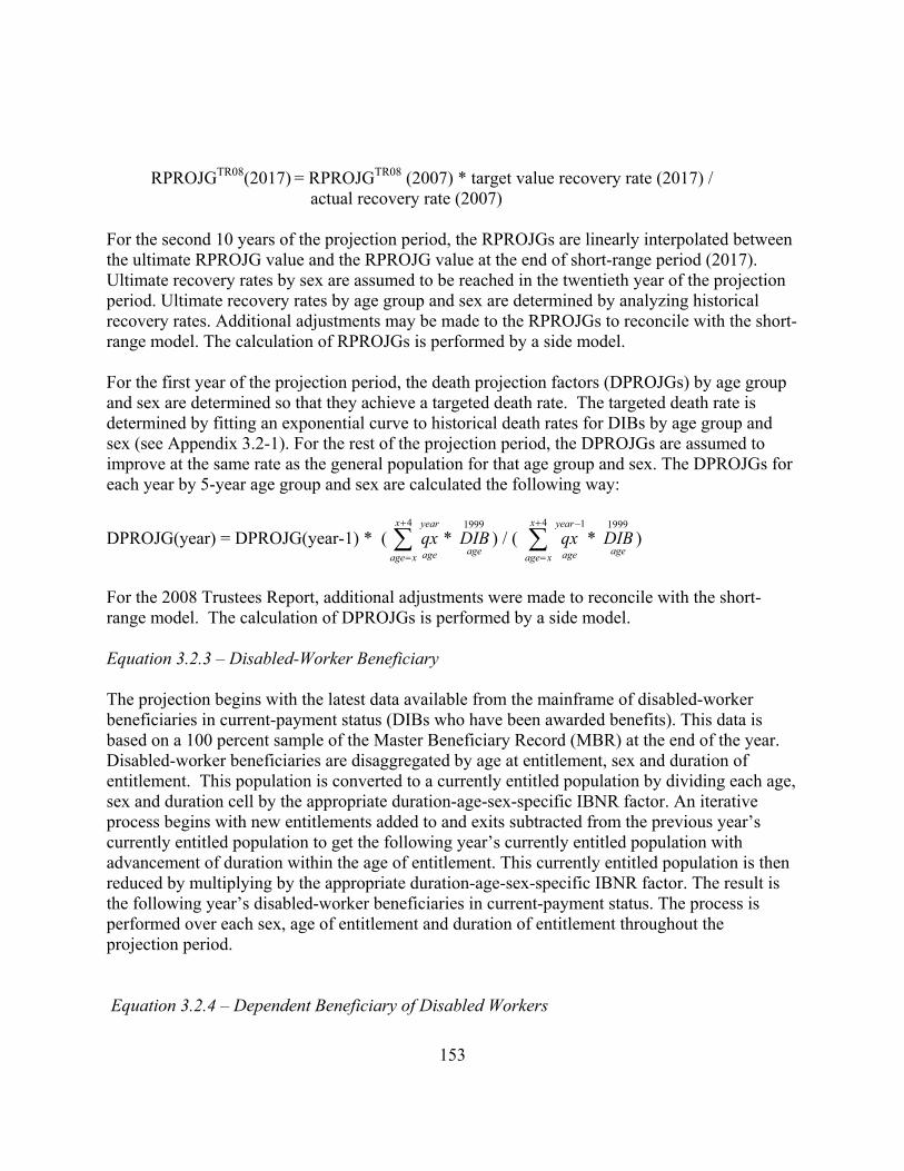
153

RPROJGTR08(2017) = RPROJGTR08 (2007) * target value recovery rate (2017) / actual recovery rate (2007) For the second 10 years of the projection period, the RPROJGs are linearly interpolated between the ultimate RPROJG value and the RPROJG value at the end of short-range period (2017). Ultimate recovery rates by sex are assumed to be reached in the twentieth year of the projection period. Ultimate recovery rates by age group and sex are determined by analyzing historical recovery rates. Additional adjustments may be made to the RPROJGs to reconcile with the short-range model. The calculation of RPROJGs is performed by a side model. For the first year of the projection period, the death projection factors (DPROJGs) by age group and sex are determined so that they achieve a targeted death rate. The targeted death rate is determined by fitting an exponential curve to historical death rates for DIBs by age group and sex (see Appendix 3.2-1). For the rest of the projection period, the DPROJGs are assumed to improve at the same rate as the general population for that age group and sex. The DPROJGs for each year by 5-year age group and sex are calculated the following way:

DPROJG(year) = DPROJG(year-1) * ( ∑+

=

4x

xage

year

ageqx *

1999

ageDIB ) / ( ∑

+

=

−4 1x

xage

year

ageqx *

1999

ageDIB )

For the 2008 Trustees Report, additional adjustments were made to reconcile with the short-range model. The calculation of DPROJGs is performed by a side model. Equation 3.2.3 – Disabled-Worker Beneficiary The projection begins with the latest data available from the mainframe of disabled-worker beneficiaries in current-payment status (DIBs who have been awarded benefits). This data is based on a 100 percent sample of the Master Beneficiary Record (MBR) at the end of the year. Disabled-worker beneficiaries are disaggregated by age at entitlement, sex and duration of entitlement. This population is converted to a currently entitled population by dividing each age, sex and duration cell by the appropriate duration-age-sex-specific IBNR factor. An iterative process begins with new entitlements added to and exits subtracted from the previous year’s currently entitled population to get the following year’s currently entitled population with advancement of duration within the age of entitlement. This currently entitled population is then reduced by multiplying by the appropriate duration-age-sex-specific IBNR factor. The result is the following year’s disabled-worker beneficiaries in current-payment status. The process is performed over each sex, age of entitlement and duration of entitlement throughout the projection period. Equation 3.2.4 – Dependent Beneficiary of Disabled Workers

154

There are six dependent-beneficiary categories; minor child, student child, disabled adult child, young spouse, married aged spouse and divorced aged spouse. Projections are disaggregated by age of the beneficiary and sex of the account holder. Presented below are the linkages and the exposure used in each of the projections of dependent beneficiaries.

Minor Child Exposure: Single SSA population by single ages 0-17 Linkages: pMCAGA = Probability that parent is under NRA

pMCDIA = Probability that parent is disability insured given that the parent is under NRA

pMCDPA = Probability that disability insured parent under NRA is disabled

MCRES = Residual Factor Student Child

Exposure: Single SSA population by single ages 18-19 Linkages: pSCAGA = Probability that parent is under NRA

pSCDIA = Probability that parent is disability insured given that the parent is under NRA

pSCDPA = Probability that disability insured parent under NRA is disabled

pSCDPC = Probability that student is in an eligible school SCRES = Residual Factor

Disabled Adult Child Exposure: Single SSA population by age groups 18-19, 20-24, 25-29,

30-34, 35-39, 40-44, 45-49, 50-54, 55-59 Linkages: pDCAGA = Probability that parent is under NRA

pDCDIA = Probability that parent is disability insured given that the parent is under NRA

pDCDPA = Probability that disability insured parent under NRA is disabled

pDCDPC = Probability that adult child is disabled DCRES = Residual Factor

Young Spouse Exposure: Married SSA population by sex and by single ages 20-64 Linkages: pYSAGA = Probability that account holder is under NRA

pYSDIA = Probability that account holder is disability insured given that the account holder is under

NRA pYSDPA = Probability that disability insured account holder

under NRA is disabled pYSETB = Probability that young spouse is not subject to earnings test pYSMCB = Probability that young spouse has a minor child

155

beneficiary in his/her care pYSDCB = Probability that young spouse has a disabled child

beneficiary in his/her care YSRES = Residual Factor

Married Aged Spouse Exposure: Married SSA population by sex and by single ages 62-100 Linkages: pMSAGA = Probability that account holder is under NRA

pMSDIA = Probability that account holder is disability insured given that the account holder is under

NRA pMSDPA = Probability that disability insured account holder

under NRA is disabled pMSFIB = Probability that beneficiary is not insured MSRES = Residual Factor

Divorced Aged Spouse Exposure: Divorced SSA population by sex and by single ages 62-100 Linkages: pDSDEA = Probability that account holder is living

pDSAGA = Probability that account holder is under NRA pDSDIA = Probability that account holder is disability

insured given that the account holder is under NRA pDSDPA = Probability that disability insured account holder

under NRA is disabled pDSFIB = Probability that beneficiary is not insured pDSDMB = Probability that beneficiary was married 10 or

more years

The residual factors for each of the dependent categories are estimated using a 10-year Least Squares regression formula. These residual factor values are then held constant for the duration of the long range period. If the 10-year Least Squares method results in a negative residual factor, the last historical residual factor is held instead. Also, APROJ factors may be developed for a dependent beneficiary category to match short range results during the first 10 years of the projection period. These factors are phased out linearly over the second ten years of the projection period.

156

Appendix: 3.2-1 The following information provides details about the regression equations used in determining incidence rates and IPROJG values by age group and sex for the first ten years of the projection period. Male Independent Variable: 16-19 unemployment rates Independent Variable: 15-19 incidence rates Dependent Variable: 15-19 incidence rates Observation Period: 1994-2004 Adjusted R square: 0.79220710 Standard Deviation: 0.27087301 Coefficient Intercept: 0.89490922 Coefficient Slope1: -0.04060960 Coefficient Slope2: 0.94206907 Independent Variable: 20-24 unemployment rates Independent Variable: 20-24 incidence rates Dependent Variable: 20-24 incidence rates Observation Period: 1994-2004 Adjusted R square: 0.71246099 Standard Deviation: 0.25579125 Coefficient Intercept: 0.17891937 Coefficient Slope1: 0.03199867 Coefficient Slope2: 0.79826938 Independent Variable: 25-29 unemployment rates Independent Variable: 25-29 incidence rates Dependent Variable: 25-29 incidence rates Observation Period: 1994-2004 Adjusted R square: 0.90460449 Standard Deviation: 0.06219117 Coefficient Intercept: 0.74487677 Coefficient Slope1: 0.17971592 Coefficient Slope2: 0.11700596 Independent Variable: 30-34 unemployment rates Independent Variable: 30-34 incidence rates Dependent Variable: 30-34 incidence rates Observation Period: 1994-2004

157

Adjusted R square: 0.85869344 Standard Deviation: 0.09561554 Coefficient Intercept: 0.39944807 Coefficient Slope1: 0.11322310 Coefficient Slope2: 0.61969161 Independent Variable: 35-39 unemployment rates Independent Variable: 35-39 incidence rates Dependent Variable: 35-39 incidence rates Observation Period: 1994-2004 Adjusted R square: 0.88647966 Standard Deviation: 0.10149922 Coefficient Intercept: 0.64066319 Coefficient Slope1: 0.23607748 Coefficient Slope2: 0.51174902 Independent Variable: 40-44 unemployment rates Independent Variable: 40-44 incidence rates Dependent Variable: 40-44 incidence rates Observation Period: 1994-2004 Adjusted R square: 0.83680625 Standard Deviation: 0.13246275 Coefficient Intercept: 1.23477573 Coefficient Slope1: 0.29462829 Coefficient Slope2: 0.45117101 Independent Variable: 45-49 unemployment rates Independent Variable: 45-49 incidence rates Dependent Variable: 45-49 incidence rates Observation Period: 1994-2004 Adjusted R square: 0.78555613 Standard Deviation: 0.16862224 Coefficient Intercept: 1.89060052 Coefficient Slope1: 0.33284681 Coefficient Slope2: 0.45768926 Independent Variable: 50-54 unemployment rates Independent Variable: 50-54 incidence rates Dependent Variable: 50-54 incidence rates Observation Period: 1994-2004 Adjusted R square: 0.79989738 Standard Deviation: 0.26552591 Coefficient Intercept: 1.49704927

158

Coefficient Slope1: 0.53085066 Coefficient Slope2: 0.63526261 Independent Variable: 55-59 unemployment rates Independent Variable: 55-59 incidence rates Dependent Variable: 55-59 incidence rates Observation Period: 1994-2004 Adjusted R square: 0.88282633 Standard Deviation: 0.29214117 Coefficient Intercept: 1.43729675 Coefficient Slope1: 0.59028867 Coefficient Slope2: 0.76646082 Independent Variable: 60-64 unemployment rates Independent Variable: 60-64 incidence rates Dependent Variable: 60-64 incidence rates Observation Period: 1994-2004 Adjusted R square: 0.78872243 Standard Deviation: 0.32769450 Coefficient Intercept: 0.66578456 Coefficient Slope1: 0.50984634 Coefficient Slope2: 0.84130036 Female Independent Variable: 16-19 unemployment rates Independent Variable: 15-19 incidence rates Dependent Variable: 15-19 incidence rates Observation Period: 1994-2004 Adjusted R square: 0.82310002 Standard Deviation: 0.17739624 Coefficient Intercept: 0.98788191 Coefficient Slope1: -0.05948284 Coefficient Slope2: 0.94114088 Independent Variable: 20-24 unemployment rates Independent Variable: 20-24 incidence rates Dependent Variable: 20-24 incidence rates Observation Period: 1994-2004 Adjusted R square: 0.75413884 Standard Deviation: 0.20229411 Coefficient Intercept: 0.26015558 Coefficient Slope1: 0.00281846 Coefficient Slope2: 0.85318973

159

Independent Variable: 25-29 unemployment rates Independent Variable: 25-29 incidence rates Dependent Variable: 25-29 incidence rates Observation Period: 1994-2004 Adjusted R square: 0.68353891 Standard Deviation: 0.16990225 Coefficient Intercept: 0.05004722 Coefficient Slope1: 0.07694539 Coefficient Slope2: 0.73561227 Independent Variable: 30-34 unemployment rates Independent Variable: 30-34 incidence rates Dependent Variable: 30-34 incidence rates Observation Period: 1994-2004 Adjusted R square: 0.77941880 Standard Deviation: 0.12190682 Coefficient Intercept: -0.02679705 Coefficient Slope1: 0.18470427 Coefficient Slope2: 0.65576148 Independent Variable: 35-39 unemployment rates Independent Variable: 35-39 incidence rates Dependent Variable: 35-39 incidence rates Observation Period: 1994-2004 Adjusted R square: 0.76781103 Standard Deviation: 0.16836691 Coefficient Intercept: 0.37840818 Coefficient Slope1: 0.28699529 Coefficient Slope2: 0.54748706 Independent Variable: 40-44 unemployment rates Independent Variable: 40-44 incidence rates Dependent Variable: 40-44 incidence rates Observation Period: 1994-2004 Adjusted R square: 0.75733974 Standard Deviation: 0.21095751 Coefficient Intercept: 0.77159180 Coefficient Slope1: 0.52415194 Coefficient Slope2: 0.42662512 Independent Variable: 45-49 unemployment rates Independent Variable: 45-49 incidence rates

160

Dependent Variable: 45-49 incidence rates Observation Period: 1994-2004 Adjusted R square: 0.80180404 Standard Deviation: 0.18259355 Coefficient Intercept: 2.61666324 Coefficient Slope1: 0.55662272 Coefficient Slope2: 0.28099690 Independent Variable: 50-54 unemployment rates Independent Variable: 50-54 incidence rates Dependent Variable: 50-54 incidence rates Observation Period: 1994-2004 Adjusted R square: 0.76597515 Standard Deviation: 0.17810560 Coefficient Intercept: 3.31718450 Coefficient Slope1: 0.45561833 Coefficient Slope2: 0.49696693 Independent Variable: 55-59 unemployment rates Independent Variable: 55-59 incidence rates Dependent Variable: 55-59 incidence rates Observation Period: 1994-2004 Adjusted R square: 0.61909066 Standard Deviation: 0.28935635 Coefficient Intercept: 5.93141485 Coefficient Slope1: 0.52684406 Coefficient Slope2: 0.45565653 Independent Variable: 60-64 unemployment rates Independent Variable: 60-64 incidence rates Dependent Variable: 60-64 incidence rates Observation Period: 1994-2004 Adjusted R square: 0.87061539 Standard Deviation: 0.20779946 Coefficient Intercept: 1.50769461 Coefficient Slope1: 0.41132859 Coefficient Slope2: 0.78037057

The following information provides details about the exponentially fitted equations used in determining death rates by age group and sex for the first year of the projection period. Male

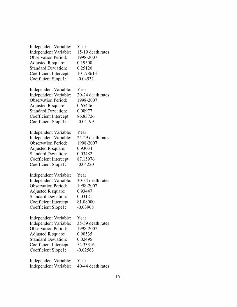
161

Independent Variable: Year Independent Variable: 15-19 death rates Observation Period: 1998-2007 Adjusted R square: 0.19500 Standard Deviation: 0.25120 Coefficient Intercept: 101.78613 Coefficient Slope1: -0.04932 Independent Variable: Year Independent Variable: 20-24 death rates Observation Period: 1998-2007 Adjusted R square: 0.65446 Standard Deviation: 0.08977 Coefficient Intercept: 86.83726 Coefficient Slope1: -0.04199 Independent Variable: Year Independent Variable: 25-29 death rates Observation Period: 1998-2007 Adjusted R square: 0.93034 Standard Deviation: 0.03482 Coefficient Intercept: 87.15976 Coefficient Slope1: -0.04220 Independent Variable: Year Independent Variable: 30-34 death rates Observation Period: 1998-2007 Adjusted R square: 0.93447 Standard Deviation: 0.03121 Coefficient Intercept: 81.08000 Coefficient Slope1: -0.03908 Independent Variable: Year Independent Variable: 35-39 death rates Observation Period: 1998-2007 Adjusted R square: 0.90535 Standard Deviation: 0.02495 Coefficient Intercept: 54.33316 Coefficient Slope1: -0.02563 Independent Variable: Year Independent Variable: 40-44 death rates

162

Observation Period: 1998-2007 Adjusted R square: 0.73605 Standard Deviation: 0.02576 Coefficient Intercept: 32.19943 Coefficient Slope1: -0.01449 Independent Variable: Year Independent Variable: 45-49 death rates Observation Period: 1998-2007 Adjusted R square: 0.71566 Standard Deviation: 0.02529 Coefficient Intercept: 30.51219 Coefficient Slope1: -0.01354 Independent Variable: Year Independent Variable: 50-54 death rates Observation Period: 1998-2007 Adjusted R square: 0.33371 Standard Deviation: 0.02162 Coefficient Intercept: 14.76689 Coefficient Slope1: -0.00559 Independent Variable: Year Independent Variable: 55-59 death rates Observation Period: 1998-2007 Adjusted R square: 0.90577 Standard Deviation: 0.01888 Coefficient Intercept: 42.66305 Coefficient Slope1: -0.01945 Independent Variable: Year Independent Variable: 60-64 death rates Observation Period: 1998-2007 Adjusted R square: 0.93276 Standard Deviation: 0.01776 Coefficient Intercept: 47.78936 Coefficient Slope1: -0.02193 Female Independent Variable: Year Independent Variable: 15-19 death rates Observation Period: 1998-2007 Adjusted R square: 0.19568

163

Standard Deviation: 0.43268 Coefficient Intercept: 173.23776 Coefficient Slope1: -0.08508 Independent Variable: Year Independent Variable: 20-24 death rates Observation Period: 1998-2007 Adjusted R square: 0.83626 Standard Deviation: 0.07498 Coefficient Intercept: 115.95251 Coefficient Slope1: -0.05657 Independent Variable: Year Independent Variable: 25-29 death rates Observation Period: 1998-2007 Adjusted R square: 0.82467 Standard Deviation: 0.05510 Coefficient Intercept: 82.47329 Coefficient Slope1: -0.03993 Independent Variable: Year Independent Variable: 30-34 death rates Observation Period: 1998-2007 Adjusted R square: 0.77932 Standard Deviation: 0.03927 Coefficient Intercept: 52.17643 Coefficient Slope1: -0.02475 Independent Variable: Year Independent Variable: 35-39 death rates Observation Period: 1998-2007 Adjusted R square: 0.86429 Standard Deviation: 0.02814 Coefficient Intercept: 50.11319 Coefficient Slope1: -0.02366 Independent Variable: Year Independent Variable: 40-44 death rates Observation Period: 1998-2007 Adjusted R square: 0.72257 Standard Deviation: 0.03335 Coefficient Intercept: 39.28514 Coefficient Slope1: -0.01815

164

Independent Variable: Year Independent Variable: 45-49 death rates Observation Period: 1998-2007 Adjusted R square: 0.86607 Standard Deviation: 0.02022 Coefficient Intercept: 37.42279 Coefficient Slope1: -0.01713 Independent Variable: Year Independent Variable: 50-54 death rates Observation Period: 1998-2007 Adjusted R square: 0.93118 Standard Deviation: 0.01745 Coefficient Intercept: 45.89877 Coefficient Slope1: -0.02128 Independent Variable: Year Independent Variable: 55-59 death rates Observation Period: 1998-2007 Adjusted R square: 0.96747 Standard Deviation: 0.01233 Coefficient Intercept: 47.94449 Coefficient Slope1: -0.02224 Independent Variable: Year Independent Variable: 60-64 death rates Observation Period: 1998-2007 Adjusted R square: 0.94734 Standard Deviation: 0.01633 Coefficient Intercept: 49.47948 Coefficient Slope1: -0.02294

165

3.3. Old-Age and Survivors Insurance 3.3.a. Overview Every month, the Social Security program pays benefits to retired workers and their dependents. It also provides benefits to eligible dependents of deceased workers. The OLD-AGE AND SURVIVORS subprocess projects the number of people expected to receive benefits over the next 75 years. The projection method is very similar to the method used for dependent beneficiaries of disabled workers in the DISABILITY subprocess. The projection of beneficiaries is computed by multiplying a subset of the Social Security area population by a series of probabilities of the conditions that a person must meet to receive benefits. The main program receives all necessary input data and performs all preliminary calculations. It then calls each individual beneficiary type subroutine where all beneficiary calculations are made. Retired workers and their dependent beneficiaries are categorized as follows:

• retired workers (RWN) by age (62-95+), sex, and marital status (single, married, widowed, divorced)

• aged spouses of retired workers (ASRWN), by age (62-95+), sex of the account holder, and marital status of the beneficiary (married, divorced)

• young spouses of retired workers (YSRWN) by age-group (under 25, 25-29,…, 65-69) and sex of the account holder

• minor, student, and disabled adult children of retired workers (MCRWN, SCRWN, and DCRWN, respectively) by age of the child (0-17 for minor, 18-19 for student, age groups 18-19, 20-24, …, 55-59, 60+ for disabled adult) and sex of the account holder

Dependent beneficiaries of deceased workers include:

• aged spouses of deceased workers, ASDWN, by age (60-95+), sex of the account holder, marital status (widowed, divorced) and insured status (insured, uninsured)

• disabled spouses of deceased workers (DSDWN) by age (50-69), sex of the account holder and marital status (widowed, divorced)

• young spouses of deceased workers (YSDWN) by age-group (under 25, 25-29,…, 65-69), sex of the account holder and marital status of the beneficiary (widowed, divorced)

• minor, student, and disabled adult children of deceased workers (MCDWN, SCDWN, and DCDWN, respectively) by age of the child (0-17 for minor, 18-19 for student, age groups 18-19, 20-24,…, 55-59, 60+ for disabled adult) and sex of the account holder

Lastly, the number of deaths of insured workers (LUMSUM) is estimated by 5-year age group (20-24, 25-29,…, 80-84, 85+) and sex.

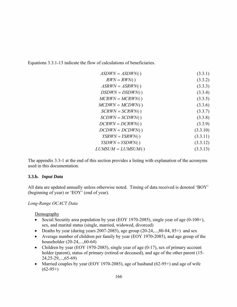
166

Equations 3.3.1-13 indicate the flow of calculations of beneficiaries.

)(⋅= ASDWNASDWN (3.3.1) )(⋅= RWNRWN (3.3.2)

)(⋅= ASRWNASRWN (3.3.3) )(⋅= DSDWNDSDWN (3.3.4) )(⋅= MCRWNMCRWN (3.3.5) )(⋅= MCDWNMCDWN (3.3.6)

)(⋅= SCRWNSCRWN (3.3.7) )(⋅= SCDWNSCDWN (3.3.8) )(⋅= DCRWNDCRWN (3.3.9) )(⋅= DCDWNDCDWN (3.3.10)

)(⋅=YSRWNYSRWN (3.3.11) )(⋅=YSDWNYSDWN (3.3.12)

)(⋅= LUMSUMLUMSUM (3.3.13) The appendix 3.3-1 at the end of this section provides a listing with explanation of the acronyms used in this documentation. 3.3.b. Input Data All data are updated annually unless otherwise noted. Timing of data received is denoted ‘BOY’ (beginning of year) or ‘EOY’ (end of year). Long-Range OCACT Data

Demography • Social Security area population by year (EOY 1970-2085), single year of age (0-100+),

sex, and marital status (single, married, widowed, divorced) • Deaths by year (during years 2007-2085), age group (20-24,...,80-84, 85+) and sex • Average number of children per family by year (EOY 1970-2085), and age group of the

householder (20-24,...,60-64) • Children by year (EOY 1970-2085), single year of age (0-17), sex of primary account

holder (parent), status of primary (retired or deceased), and age of the other parent (15-24,25-29,...,65-69)

• Married couples by year (EOY 1970-2085), age of husband (62-95+) and age of wife (62-95+)

167

• Persons with an aged spouse by year (EOY 1970-2085), age group (15-24, 25-29,...,65-69) and sex

Economics • Covered wages and employment in the Federal Civilian and State and Local Sectors

(during years 1998-2085) • Labor force participation rates for age 62 by year (during years 1970-2085) and sex Beneficiaries • Fully insured persons by year (EOY 1970-2085), age (14-95+), sex, and marital status

(single, married, widowed, divorced) • Disabled-worker beneficiaries in current pay by year (EOY 1970-2085), age (62-66) and

sex • Converted DI to OAI beneficiaries by year (EOY 1970-2085), age(65-95+) and sex • Disability prevalence rates by year (EOY 1970-2085), age (50-66) and sex

Short-Range OCACT Data

• Insured aged spouses of deceased workers by year (EOY 1998-2007), age (60-95+) and sex

• The following is received for EOY 2006 and 2007:

a. Aged spouses of deceased workers by age (60-95+), sex and marital status (widowed, divorced)

b. Retired workers by age (62-95+) and sex c. Aged spouses of retired workers by age (62-95+), sex and marital status (married,

divorced) d. Disabled widow(er)s by age (50-64), sex and marital status (widowed, divorced) e. Minor children by age (0-17), sex of parent and status of parent (retired, deceased) f. Student children by age (18-19), sex of parent and status of parent (retired, deceased) g. Disabled adult children by age (20-95+), sex of parent and status of parent (retired,

deceased) h. Young spouses of retired workers by age group (under 25, 25-29,...,60-64) and sex i. Young spouses of deceased workers by age group (under 25, 25-29,...,65-69), sex and

marital status (widowed, divorced) j. Total parent beneficiaries Note: Each year, data for the most recent historical year is appended.

• The following is received for EOY 2017:

a. Retired workers by age group (62-64, 65-69) and sex b. Insured widows by age group (60-64,...,80-84,85+) c. Uninsured widows by age group (60-64, 65+) d. Total disabled widows

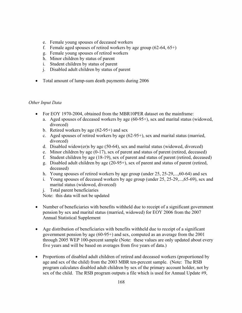
168

e. Female young spouses of deceased workers f. Female aged spouses of retired workers by age group (62-64, 65+) g. Female young spouses of retired workers h. Minor children by status of parent i. Student children by status of parent j. Disabled adult children by status of parent

• Total amount of lump-sum death payments during 2006

Other Input Data

• For EOY 1970-2004, obtained from the MBR10PER dataset on the mainframe: a. Aged spouses of deceased workers by age (60-95+), sex and marital status (widowed,

divorced) b. Retired workers by age (62-95+) and sex c. Aged spouses of retired workers by age (62-95+), sex and marital status (married,

divorced) d. Disabled widow(er)s by age (50-64), sex and marital status (widowed, divorced) e. Minor children by age (0-17), sex of parent and status of parent (retired, deceased) f. Student children by age (18-19), sex of parent and status of parent (retired, deceased) g. Disabled adult children by age (20-95+), sex of parent and status of parent (retired,

deceased) h. Young spouses of retired workers by age group (under 25, 25-29,...,60-64) and sex i. Young spouses of deceased workers by age group (under 25, 25-29,...,65-69), sex and

marital status (widowed, divorced) j. Total parent beneficiaries Note: this data will not be updated

• Number of beneficiaries with benefits withheld due to receipt of a significant government

pension by sex and marital status (married, widowed) for EOY 2006 from the 2007 Annual Statistical Supplement

• Age distribution of beneficiaries with benefits withheld due to receipt of a significant

government pension by age (60-95+) and sex, computed as an average from the 2001 through 2005 WEP 100-percent sample (Note: these values are only updated about every five years and will be based on averages from five years of data.)

• Proportions of disabled adult children of retired and deceased workers (proportioned by

age and sex of the child) from the 2003 MBR ten-percent sample. (Note: The RSB program calculates disabled adult children by sex of the primary account holder, not by sex of the child. The RSB program outputs a file which is used for Annual Update #9,

169

which calculates beneficiaries by sex. Therefore the 2003 proportions are applied to estimate the breakdown of disabled adult children by sex of the child. This input file will not be updated.)

• Schedule of normal retirement age (NRA), delayed retirement credit, and actuarial

reduction factors for ages more than 3 years below NRA and less than 3 years below NRA for years 1970-2085 from the Social Security website (Note: these values are only updated when there is a Social Security law change regarding the NRA)

• Elasticity factors by age (65-69) and sex for the elimination of the earnings test after

NRA • Prevalence rate regression coefficients (slope and y-intercept value by sex) • Regressed prevalence rate by sex for the most recent historical year • Adjustment factors which account for the difference between estimated and actual

historical retired worker prevalence rates by year (EOY 1970-2085), age (63-69) and sex • Adjustment factors which account for the difference between projected beneficiary values

for the tenth year of the projection period made by the Long-Range and Short-Range offices. Factors are computed for: a. Retired workers by age group (62-64, 65-69) and sex b. Insured widows by age group (60-64,...,80-84,85+) c. Uninsured widows by age group (60-64, 65+) d. Total disabled widows e. Female young spouses of deceased workers f. Female aged spouses of retired workers by age group (62-64, 65+) g. Female young spouses of retired workers h. Minor children by status of parent i. Student children by status of parent j. Disabled adult children by status of parent

3.3.c. Development of Output Several acronyms are used to describe the equations presented below. Acronyms that are not preceded with a subscript generally refer to the number of beneficiaries. For example, RWN refers to the number of retired workers. Acronyms that are preceded with a ‘p’ refer to probabilities. For example, FIApRW refers to the probability that a person is fully insured. Equation 3.3.1 – Aged Spouses of Deceased Workers (ASDWN)

170

The number of aged spouses of deceased workers (widow(er)s), along with all linkage factors, are projected by age, sex of the account holder (sa=1 for male, sa=2 for female), marital status and insured status. Age ranges from 60 to 95+, marital status includes widowed (mb=1) and divorced (mb=2), and insured status includes insured (in=1) and uninsured (in=2). Note that for all variables, a subscript of p denotes that the variable is a calculated probability. The projected number of aged spouses of deceased workers is calculated as follows:

RESGPBFIB

MBBFIADEAPOP

pASDWpASDWpASDWpASDWpASDWpASDWASDWASDWN

∗∗∗∗∗∗=

(3.3.1)

ASDWPOP represents the subset of the population from which these beneficiaries are drawn and is set equal to the Social Security area population (SSAPOPmb) for each possible marital status.

mbPOP SSAPOPASDW =

pASDWDEA represents the probability that the primary account holder (PAH) is deceased. For the widowed population, this factor is set equal to one. For the divorced population, this factor is set equal to the portion of the total widowed (SSAPOPwid) and married (SSAPOPmar) population who are widowed. 1 , mb=1 (widowed)

widmar

wid

SSAPOPSSAPOPSSAPOP

+ , mb=2 (divorced)

pASDWFIA represents the probability that the PAH was fully insured at death. For a given age of widow, AW, it is assumed that the age of her deceased husband, AH, ranges from AW-6 to AW+12 with a lower and upper bound of 60 and 95+. Further, it is assumed that the more likely age of the husband is AW+3. For each age, pASDWFIA is calculated as a weighted average of the portion of the Social Security area population who are fully insured at each possible age of the husband (FINSAH). For example, for a widow age 70, it is assumed that the age of her husband is between 64 and 82, therefore the weighted average of the portion of the population who are fully insured males is calculated, applying the highest weight of 10 to age 73, and a linearly reduced weight to zero for each age above and below 73. The same concept is used for widow(er)s with the assumption that the age of his deceased wife ranges from AH-12 to AH+6, with a greater likelihood of her age being AH-3. Let WEIGHT represent the specific weight applied to each potential age of the spouse.

AHAWWEIGHTAH −+−= 310

pASDWDEA =

171

AWAHWEIGHTAW −−−= 310

∑

∑+

−=

+

−=

∗

12

6

12

6AW

AWAHAH

AW

AWAHAHAH

WEIGHT

FINSWEIGHT, sa=1

pASDWFIA =

∑

∑+

−=

+

−=

∗

6

12

6

12AH

AHAWAW

AH

AHAWAWAW

WEIGHT

FINSWEIGHT, sa=2

pASDWMBB represents the probability that the widow(er) is not receiving a young-spouse benefit for the care of a child. A young-spouse benefit can be received up to age 69 if all other eligibility requirements are met. Since the minimum age requirement to receive a widow(er) benefit is 60, it is necessary to remove those receiving a young-spouse benefit ( abYSDWN ), where ab represents the 5-year age bracket39. A uniform breakdown is assumed to divide the age groups into single-age estimates.

1 , 65≤age<NRA and in=2

0 , elsewhere

FIADEAPOP pASDWpASDWASDW

YSDWN∗∗

∗−

−64602.01

∑∗

∗∗−

−

69

65

6965

1age

age

FIADEAPOP FACTOR

FACTORpASDWpASDWASDW

YSDWN

1

pASDWFIB represents the probability that the aged widow(er) is fully insured. For insured widow(er)s, pASDWFIB is the portion of the Social Security area population that is fully insured (FINS) at each age, sex, and marital status. For uninsured widow(er)s, pASDWFIB is simply one minus the probability for insured widow(er)s.

39 There are no young spouses at NRA or above.

pASDWMBB = , 65≤age<NRA and in=2

FACTORage =

, age=60-64 and in=2

, age=60-69 and in=1

172

mbSSAPOP

FINS , in=1

pASDWFIB =

mbSSAPOP

FINS−1 , in=2

pASDWGPB represents the probability that the aged-widow(er)'s benefits are not withheld or not offset totally because of receipt of a significant government pension based on earnings in noncovered employment. According to the 1977 amendment, the Social Security benefits are subject to reduction by up to two-thirds of non-covered government pensions. GPWHLD represents the total number of widow(er) beneficiaries (for all ages) expected to receive a significant government pension. rGPOAGE represents the ratio of the total for each given age. If a person is insured, this implies that he/she is eligible to receive Social Security benefits based on his/her own earnings regardless of a government pension. Therefore no factor is applied.

1

FIBMBBFIADEAPOP pASDWpASDWpASDWpASDWASDW

GPWHLDrGPOAGE∗∗∗∗

∗−1 , in=2

pASDWRES represents the probability that a widow(er) eligible to receive widow(er)’s benefits, would actual receive the benefits. In particular, for in=1, this factor is equivalent to the probability that a widow(er) eligible to receive his/her own retired-worker benefits would instead apply for and receive widow(er) benefits. For all historical years, year

RESpASDW is calculated as the ratio of ASDWN, the actual number of widow(er)s, to the number of persons meeting all previously mentioned requirements by age, sex, insured status, and marital status.

GPBFIBMBBFIADEAPOP

yearRES pASDWpASDWpASDWpASDWpASDWASDW

ASDWNpASDW∗∗∗∗∗

=

where TRYR is the Trustees Report year. For each age, sex, insured status, and marital status, a least squares regression is used over the last ten years of historical data to determine a starting value in TRYR-1 for

yearRESpASDW from which future values are projected. In addition, for each sex, insured status,

and marital status, the regressed values of 1−TRYRRESpASDW are graduated over age using a

weighted minimized third-difference formula to produce ASDWESTRES . ASDWESTRES are the preliminary estimates of 9+TRYR

RESpASDW , the values in the tenth year of the projection period. In addition, adjustments by age group (60-64, 65-69, 70-74, 75-79, 80-84, 85+ for insured;

pASDWGPB =

, year<TRYR,

, in=1 OR year≤1978

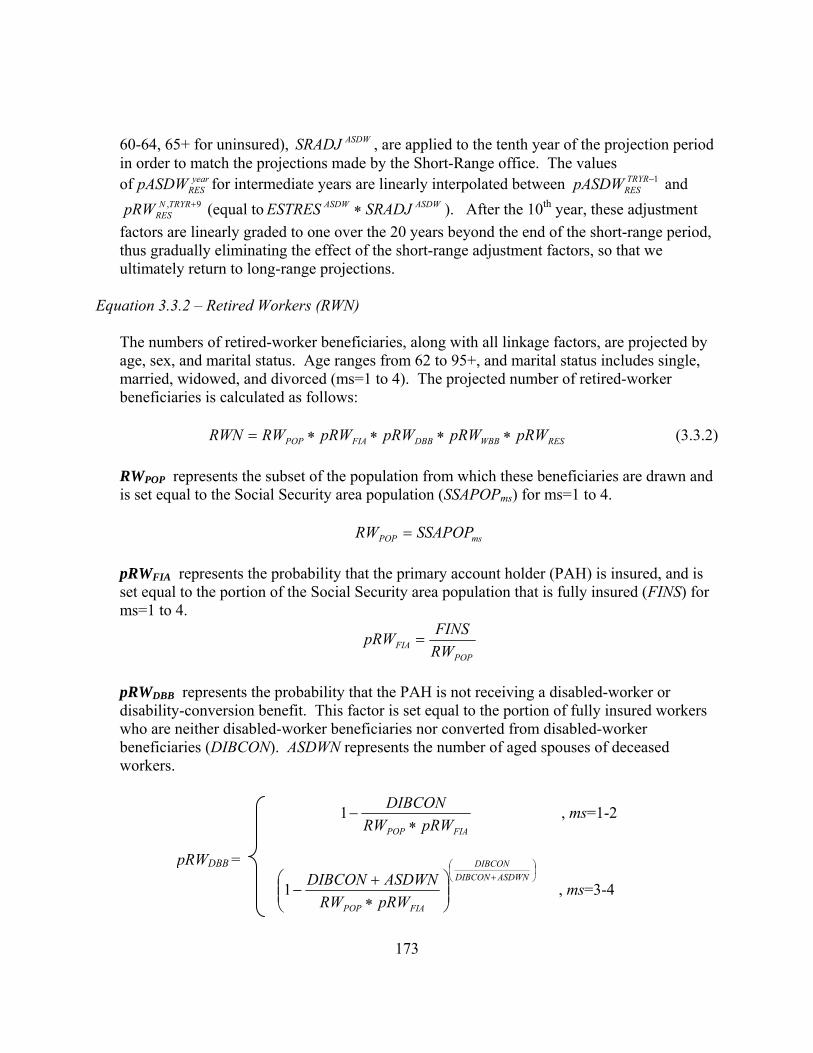
173

60-64, 65+ for uninsured), ASDWSRADJ , are applied to the tenth year of the projection period in order to match the projections made by the Short-Range office. The values of year

RESpASDW for intermediate years are linearly interpolated between 1−TRYRRESpASDW and

9, +TRYRNRESpRW (equal to ASDWASDW SRADJESTRES ∗ ). After the 10th year, these adjustment

factors are linearly graded to one over the 20 years beyond the end of the short-range period, thus gradually eliminating the effect of the short-range adjustment factors, so that we ultimately return to long-range projections.

Equation 3.3.2 – Retired Workers (RWN)

The numbers of retired-worker beneficiaries, along with all linkage factors, are projected by age, sex, and marital status. Age ranges from 62 to 95+, and marital status includes single, married, widowed, and divorced (ms=1 to 4). The projected number of retired-worker beneficiaries is calculated as follows:

RESWBBDBBFIAPOP pRWpRWpRWpRWRWRWN ∗∗∗∗= (3.3.2)

RWPOP represents the subset of the population from which these beneficiaries are drawn and is set equal to the Social Security area population (SSAPOPms) for ms=1 to 4.

msPOP SSAPOPRW = pRWFIA represents the probability that the primary account holder (PAH) is insured, and is set equal to the portion of the Social Security area population that is fully insured (FINS) for ms=1 to 4.

POPFIA RW

FINSpRW =

pRWDBB represents the probability that the PAH is not receiving a disabled-worker or disability-conversion benefit. This factor is set equal to the portion of fully insured workers who are neither disabled-worker beneficiaries nor converted from disabled-worker beneficiaries (DIBCON). ASDWN represents the number of aged spouses of deceased workers.

FIAPOP pRWRW

DIBCON∗

−1 , ms=1-2

⎟⎠⎞

⎜⎝⎛

+

⎟⎟⎠

⎞⎜⎜⎝

⎛∗+

−ASDWNDIBCON

DIBCON

FIAPOP pRWRWASDWNDIBCON1 , ms=3-4

pRWDBB =

174

pRWWBB represents the probability that the PAH is not receiving a widow(er) benefit, and is set equal to the portion of fully insured workers that is not aged spouses of deceased workers. 1 , ms=1-2

⎟⎠⎞

⎜⎝⎛

+

⎟⎟⎠

⎞⎜⎜⎝

⎛∗+

−ASDWNDIBCON

ASDWN

FIAPOP pRWRWASDWNDIBCON1 , ms=3-4

pRWRES

N,year represents the retirement prevalence rate, which is the probability that a fully insured worker not receiving disability or widow(er)’s benefits would receive retired-worker benefits as of the given age, N, for the given year. In order to estimate the future prevalence rate, the program first calculates the historical values of yearN

RESpRW , . For each historical year and sex, yearN

RESpRW , is calculated as the ratio of RWN, the actual number of retired workers, to the number of persons meeting all previously mentioned requirements by age, sex, and marital status.

WBBDBBFIAPOP

yearNRES pRWpRWpRWRW

RWNpRW∗∗∗

=, , N=62-95+ and year<TRYR

Historical prevalence rates at age 62 and labor force participation rates (LFPRyear) at age 62, by sex, follow an inverse linear relationship over the historical period. This relationship is assumed to hold in the projection period, and therefore used to calculate REGPRyear, the regressed prevalence rate based on the projected LFPRyear at age 62 for each year and sex. Note that prevalence rates are calculated on a cohort basis40. The regression equation used to estimate the prevalence rates is:

91421.0*97734.0 +−= yearyear LFPRREGPR for male with an R2 value of 0.92637, and

76193.0*78782.0 +−= yearyear LFPRREGPR for female with an R2 value of 0.78454. The future prevalence rate at age 62, year

RESpRW ,62 , is then set equal to the sum of the regressed prevalence rate (REGPRyear) and ERROR, the difference between the actual prevalence rate and the regressed prevalence rate in the most recent historical year, which is phased out linearly.

40 For example, to calculate the projected number of 65 year olds in a given year, the prevalence rate at age 62 is needed. This is actually the prevalence rate that occurred three years ago at age 62.

pRWWBB

175

⎟⎠⎞

⎜⎝⎛ −+

∗+=109,0max)(,62 yearTRYRERRORREGPRpRW yearyear

RES

To compute yearN

RESpRW , for ages 63 to 69 in the projection period, several preliminary variables must be calculated. These include:

MBAPIAN, for N=62,70 (same for both sexes), year

NESTPR , for N=63,69 and by sex, DIFFADJN, for N=63,69 and by sex, year

NESTPR2 for N=63,69 and by sex, and EARNN, for N=65,69 and by sex.

MBAPIAN is the ratio of the monthly benefit amount (MBA) to the primary insurance amount (PIA) at age N and is calculated on a cohort basis for N=62,70. The calculation of MBAPIAN is based on the normal retirement age (NRA), delayed retirement credits (DRC), and actuarial reduction factors; ARFLE3 when the difference between NRA and age at retirement is less than 3, and ARFGT3 when the difference is greater than 3 within each cohort. If a person retires after NRA, his/her benefits are increased by DRC for each year the age exceeds NRA. If a person retires before NRA, his/her benefits are decreased by ARFLE3 for each of the first three years that NRA exceeds the age, and further decreased by ARFGT3 for any remaining years.

DRCNRAN ∗−+ )(1 , N≥NRA 3)(1 ARFLENNRA ∗−− , NRA-3≤N<NRA 3)3(331 ARFGTNNRAARFLE ∗−−−∗− , N<NRA-3

yearNESTPR , the estimated prevalence rate at age N, is then calculated as the prevalence rate

at age 62 ( )62(,62 −− NyearRESpRW ) plus an estimate on the expected portion of the remaining

probability ( )62(,621 −−− NyearRESpRW ), that a potential retired worker will actually retire by that

given age. This estimate is based on MBAPIAN, assuming that the retirement decision by a worker is totally and completely influenced by the expected change in the portion of PIA that is payable at each age relative to the potential change after the initial eligibility.

6270

62)62(,62)62(,62 )1(MBAPIAMBAPIAMBAPIAMBAPIA

pRWpRWESTPR NNyearRES

NyearRES

yearN −

−∗−+= −−−−

In the first year of the projection period, an adjustment (DIFFADJN) is made which accounts for the difference between the actual and estimated prevalence rate at each age in the most recent historical years; For ages 63 and 64, the value used beginning in TRYR is the average of the last 5 years’ differences between the actual and estimated PR. This value is held

MBAPIAN =

, N=62 and year≥TRYR-1

, N=63-69

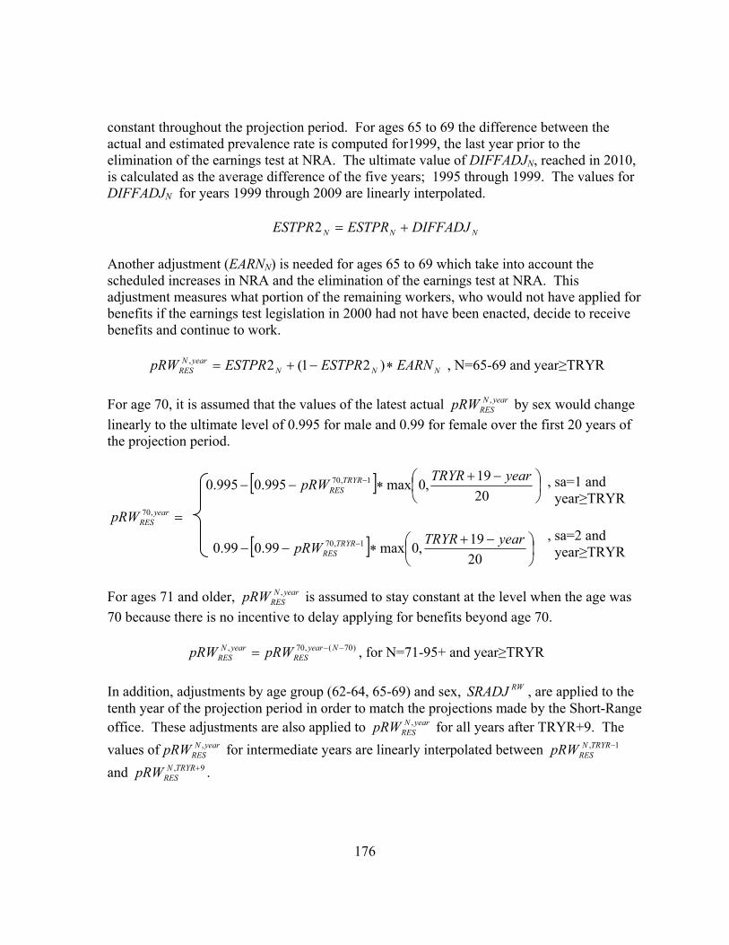
176

constant throughout the projection period. For ages 65 to 69 the difference between the actual and estimated prevalence rate is computed for1999, the last year prior to the elimination of the earnings test at NRA. The ultimate value of DIFFADJN, reached in 2010, is calculated as the average difference of the five years; 1995 through 1999. The values for DIFFADJN for years 1999 through 2009 are linearly interpolated.

NNN DIFFADJESTPRESTPR +=2

Another adjustment (EARNN) is needed for ages 65 to 69 which take into account the scheduled increases in NRA and the elimination of the earnings test at NRA. This adjustment measures what portion of the remaining workers, who would not have applied for benefits if the earnings test legislation in 2000 had not have been enacted, decide to receive benefits and continue to work.

NNNyearN

RES EARNESTPRESTPRpRW ∗−+= )21(2, , N=65-69 and year≥TRYR For age 70, it is assumed that the values of the latest actual yearN

RESpRW , by sex would change linearly to the ultimate level of 0.995 for male and 0.99 for female over the first 20 years of the projection period.

[ ] ⎟⎠⎞

⎜⎝⎛ −+

∗−− −

2019,0max995.0995.0 1,70 yearTRYRpRW TRYR

RES

=yearRESpRW ,70

[ ] ⎟⎠⎞

⎜⎝⎛ −+

∗−− −

2019,0max99.099.0 1,70 yearTRYRpRW TRYR

RES

For ages 71 and older, yearN

RESpRW , is assumed to stay constant at the level when the age was 70 because there is no incentive to delay applying for benefits beyond age 70.

)70(,70, −−= Nyear

RESyearN

RES pRWpRW , for N=71-95+ and year≥TRYR

In addition, adjustments by age group (62-64, 65-69) and sex, RWSRADJ , are applied to the tenth year of the projection period in order to match the projections made by the Short-Range office. These adjustments are also applied to yearN

RESpRW , for all years after TRYR+9. The values of yearN

RESpRW , for intermediate years are linearly interpolated between 1, −TRYRNRESpRW

and 9, +TRYRNRESpRW .

, sa=1 and year≥TRYR

, sa=2 and year≥TRYR

177

For each age, retired workers are further broken down by age at entitlement, AE, by multiplying the number of retired workers at age N by the ratio of the incidence rate at AE (N-AE years prior) to the prevalence rate at age N.

yearNRES

AENyearAEyearNyearN

AE pRWINCRATERWNRWN ,

)(

*−−

= , AE≤N

where the incidence rate for a given AE=N and year is calculated as the change in the prevalence rate at age N to the prevalence rate at age N-1 in the previous year. yearN

RESpRW , , for N=AE=62 =year

AE INCRATE 1,1, −−− yearNRES

yearNRES pRWpRW , for 63≤N=AE≤69

1,11 −−− yearN

RESpRW , for N=AE=70

Equation 3.3.3 – Aged Spouses of Retired Workers (ASRWN)

The number of aged spouses of retired workers, along with all linkage factors, are projected by age, sex of the account holder (sa=1,2), and marital status of the beneficiary. Age ranges from 62 to 95+, and marital status includes married (mb=1) and divorced (mb=2). The projected number of aged spouses of retired workers is calculated as follows:

RESGPBFIBMBB

CPAFIAAGADEAPOP

pASRWpASRWpASRWpASRWpASRWpASRWpASRWpASRWASRWASRWN

∗∗∗∗∗∗∗∗=

(3.3.3)

ASRWPOP represents the subset of the population from which these beneficiaries are drawn and is set equal to the Social Security area population (SSAPOPmb) for mb=1,2.

mbPOP SSAPOPASRW = pASRWDEA represents the probability that the PAH is not deceased. For the married population, no factor is applied. For the divorced population, the factor is set equal to the portion of the total married and widowed population who are married. 1 , mb=1 (married)

178

widmar

mar

SSAPOPSSAPOPSSAPOP

+ , mb=2 (divorced)

pASRWAGA represents the probability that the PAH is of the required age, and is set equal to the portion of the married population with a spouse (PAH) at least age 62 (MAR62PLUS).

pASRWAGA = marSSAPOP

PLUSMAR62

pASRWFIA represents the probability that the PAH is fully insured, and is set equal to the portion of married couples of the required age where the PAH is fully insured (FI_PAH). For example, when the program is estimating the number of female aged spouse of retired workers, this factor will find the portion where their spouse, the male PAH, is fully insured.

[ ]∑

∑ ∗=

PLUSMARPAHFIPLUSMAR

pASRWFIA 62_62

pASRWCPA represents the probability that the PAH is receiving benefits. This factor is set equal to the portion of eligible married couples where the PAH is receiving benefits (RETIRED). If the beneficiary is divorced, no factor is applied, since it is not required for the retired worker to be receiving benefits for the divorced aged spouse to receive benefits. 1 , year ≥1985 and mb=2

[ ]

[ ]∑∑

∗

∗∗

PAHFIPLUSMARRETIREDPAHFIPLUSMAR

_62_62

, elsewhere

pASRWMBB represents the probability that the beneficiary is not receiving a young-spouse benefit. If the beneficiary is age 70 or older or if the beneficiary is divorced, no factor is applied. Otherwise, this factor is set equal to the portion of potentially eligible widow(er)s where the spouse of the PAH is not receiving a young-spouse benefit ( abYSRWN ), where ab represents the 5-year age group.41

1 , 65≤age<NRA

0 , elsewhere 41 There are no young spouses at NRA or above.

pASRWDEA =

pASRWCPA =

FACTORage =

179

CPAFIAAGADEAPOP pASRWpASRWpASRWpASRWASRW

YSRWN∗∗∗∗

∗−

−64602.01

∑∗

∗∗∗∗−

−

69

65

6965

1

ag

ag

CPAFIAAGADEAPOP

FACTOR

FACTOR

pASRWpASRWpASRWpASRWASRWYSRWN

1 , elsewhere pASRWFIB represents the probability that the aged spouse is not fully insured, and is therefore not receiving a retired-worker benefit based on his/her own earnings. This factor is set equal to the portion of the married and divorced population that is not fully insured. For example, when the program is estimating the number of female aged spouse of retired workers, this factor will find the portion of female beneficiaries that is fully insured.

SSAPOPFINSpASRWFIB −= 1 , mb=1-2

pASRWGPB represents the probability that the aged-spouse's benefits are not withheld because of receipt of a significant government pension based on earnings in noncovered employment. GPWHLD represents the total number of aged spouse of retired-worker beneficiaries (for all ages) expected to receive a significant government pension. rGPOAGE represents the ratio of the total for each given age. 1 , year≤1978

FIBCPAFIAAGADEAPOP pASRWpASRWpASRWpASRWpASRWASRWGPWHLDrGPOAGE

∗∗∗∗∗∗

−1 , elsewhere

pASRWMBB =

, age=62-64 and mb=1

, 65≤age<NRA and mb=1

pASRWGPB =

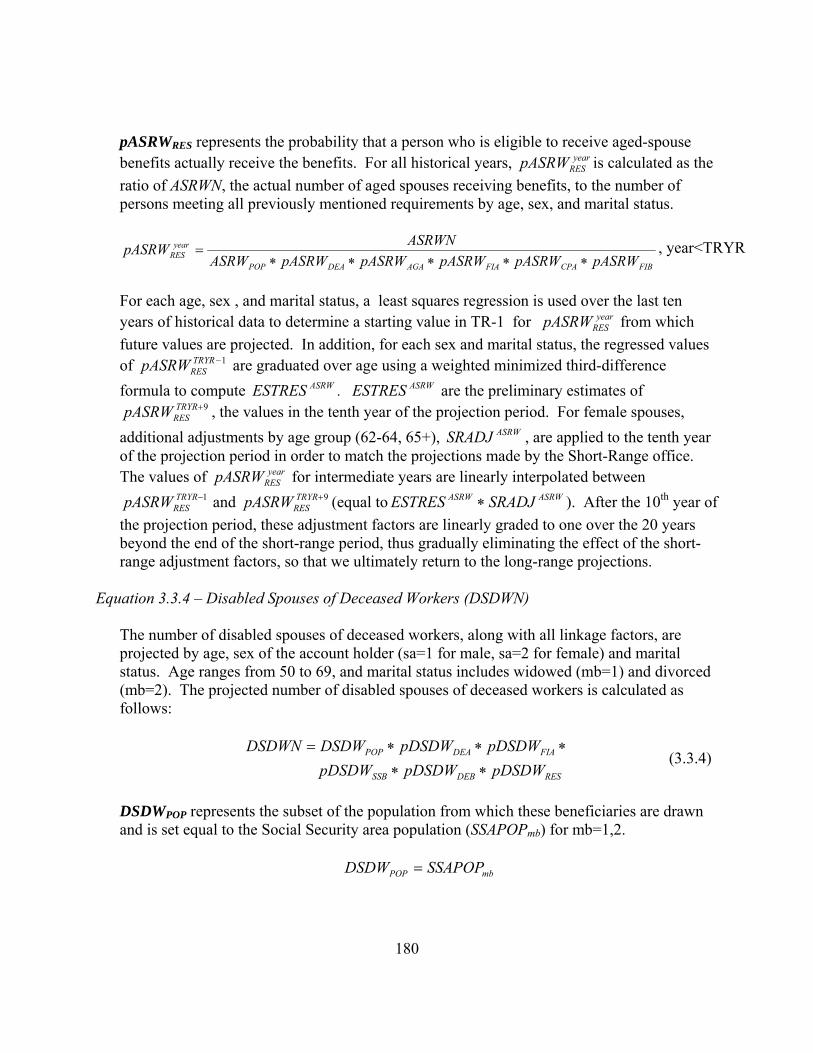
180

pASRWRES represents the probability that a person who is eligible to receive aged-spouse benefits actually receive the benefits. For all historical years, year

RESpASRW is calculated as the ratio of ASRWN, the actual number of aged spouses receiving benefits, to the number of persons meeting all previously mentioned requirements by age, sex, and marital status.

FIBCPAFIAAGADEAPOP

yearRES pASRWpASRWpASRWpASRWpASRWASRW

ASRWNpASRW∗∗∗∗∗

=

For each age, sex , and marital status, a least squares regression is used over the last ten years of historical data to determine a starting value in TR-1 for year

RESpASRW from which future values are projected. In addition, for each sex and marital status, the regressed values of 1−TRYR

RESpASRW are graduated over age using a weighted minimized third-difference formula to compute ASRWESTRES . ASRWESTRES are the preliminary estimates of

9+TRYRRESpASRW , the values in the tenth year of the projection period. For female spouses,

additional adjustments by age group (62-64, 65+), ASRWSRADJ , are applied to the tenth year of the projection period in order to match the projections made by the Short-Range office. The values of year

RESpASRW for intermediate years are linearly interpolated between 1−TRYR

RESpASRW and 9+TRYRRESpASRW (equal to ASRWASRW SRADJESTRES ∗ ). After the 10th year of

the projection period, these adjustment factors are linearly graded to one over the 20 years beyond the end of the short-range period, thus gradually eliminating the effect of the short-range adjustment factors, so that we ultimately return to the long-range projections.

Equation 3.3.4 – Disabled Spouses of Deceased Workers (DSDWN)

The number of disabled spouses of deceased workers, along with all linkage factors, are projected by age, sex of the account holder (sa=1 for male, sa=2 for female) and marital status. Age ranges from 50 to 69, and marital status includes widowed (mb=1) and divorced (mb=2). The projected number of disabled spouses of deceased workers is calculated as follows:

RESDEBSSB

FIADEAPOP

pDSDWpDSDWpDSDWpDSDWpDSDWDSDWDSDWN∗∗

∗∗∗= (3.3.4)

DSDWPOP represents the subset of the population from which these beneficiaries are drawn and is set equal to the Social Security area population (SSAPOPmb) for mb=1,2.

mbPOP SSAPOPDSDW =

, year<TRYR

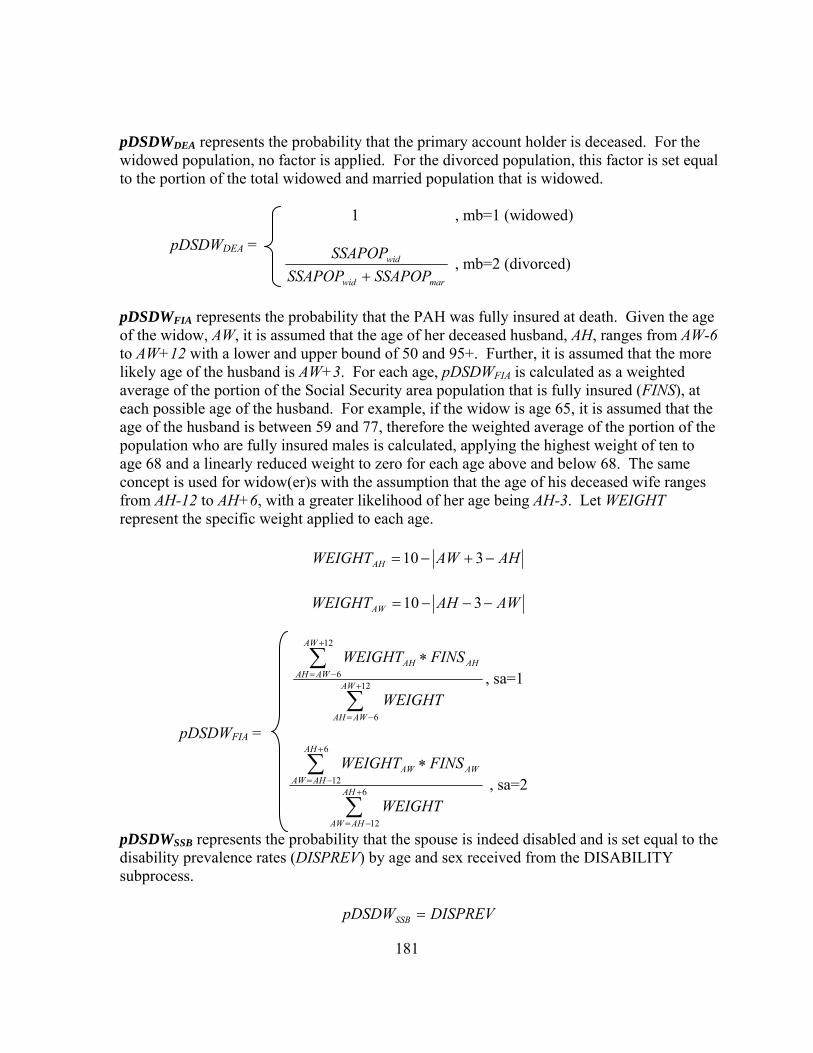
181

pDSDWDEA represents the probability that the primary account holder is deceased. For the widowed population, no factor is applied. For the divorced population, this factor is set equal to the portion of the total widowed and married population that is widowed. 1 , mb=1 (widowed)

marwid

wid

SSAPOPSSAPOPSSAPOP

+ , mb=2 (divorced)

pDSDWFIA represents the probability that the PAH was fully insured at death. Given the age of the widow, AW, it is assumed that the age of her deceased husband, AH, ranges from AW-6 to AW+12 with a lower and upper bound of 50 and 95+. Further, it is assumed that the more likely age of the husband is AW+3. For each age, pDSDWFIA is calculated as a weighted average of the portion of the Social Security area population that is fully insured (FINS), at each possible age of the husband. For example, if the widow is age 65, it is assumed that the age of the husband is between 59 and 77, therefore the weighted average of the portion of the population who are fully insured males is calculated, applying the highest weight of ten to age 68 and a linearly reduced weight to zero for each age above and below 68. The same concept is used for widow(er)s with the assumption that the age of his deceased wife ranges from AH-12 to AH+6, with a greater likelihood of her age being AH-3. Let WEIGHT represent the specific weight applied to each age.

AHAWWEIGHTAH −+−= 310

AWAHWEIGHTAW −−−= 310

∑

∑+

−=

+

−=

∗

12

6

12

6AW

AWAH

AW

AWAHAHAH

WEIGHT

FINSWEIGHT, sa=1

pDSDWFIA =

∑

∑+

−=

+

−=

∗

6

12

6

12AH

AHAW

AH

AHAWAWAW

WEIGHT

FINSWEIGHT , sa=2

pDSDWSSB represents the probability that the spouse is indeed disabled and is set equal to the disability prevalence rates (DISPREV) by age and sex received from the DISABILITY subprocess.

DISPREVpDSDWSSB =

pDSDWDEA =

182

pDSDWDEB represents the probability that the disabled spouse is not dually eligible for another type of benefit. This factor is assumed to remain at a constant level by sex. 0.85 , sa=1 pDSDWDEB = 0.06 , sa=2 pDSDWRES represents the probability that a person who is eligible to receive disabled-spouse benefits actually receive the benefits. For all historical years, year

RESpDSDW is calculated as the ratio of DSDWN, the actual number of disabled spouses of deceased workers receiving benefits, to the number of persons meeting all previously mentioned requirements by age, sex, and marital status.

DEBFIADEAPOP

yearRES pDSDWpDSDWpDSDWDSDW

DSDWNpDSDW∗∗∗

= , year<TRYR

For ages 50 to 64, and each sex, and marital status, a least squares regression is used over the last ten years of historical data to determine a starting value in TR-for year

RESpDSDW from which future values are projected. In addition, for each sex and marital status, the regressed values of 1−TRYR

RESpDSDW are graduated over age using a weighted minimized third-difference formula to compute DSDWESTRES . DSDWESTRES are the preliminary estimates of

9+TRYRRESpDSDW , the values in the tenth year of the projection period. For female disabled

spouses, an adjustment, DSDWSRADJ , is applied to the tenth year of the projection period in order to match the projections made by the Short-Range office. The values of

yearRESpDSDW for intermediate years are exponentially interpolated between 1−TRYR

RESpDSDW and 9+TRYR

RESpDSDW (equal to DSDWDSDW SRADJESTRES ∗ ). After the 10th year of the projection period, the adjustment factors are linearly graded to one over the 20 years beyond the end of the short-range period, thus gradually eliminating the effect of the short-range adjustment factors, so that we ultimately return to the long-range projections.

For the projection period, for ages 65 to 69 where age is less than NRA, year

RESpDSDW is equal to year

RESpDSDW at age 64 times an adjustment which accounts for the additional ages as NRA changes.

1 , NRA≥age+1

NRA-age , age<NRA<age+1

FACTORage =

183

age

age

yearRES

yearRESyear

RESyear

RES FACTORpDSDWpDSDW

pDSDWpDSDW ∗⎟⎟⎠

⎞⎜⎜⎝

⎛∗=

− )64(

63,

64,64,

Equation 3.3.5-6 – Minor Children of Retired and Deceased Workers (MCRWN and MCDWN )

The number of minor children of retired workers, MCRWN, is projected by age of the minor (am=0 to 17) and sex of the account holder (sa=1 for male, sa=2 for female), and is calculated by multiplying the number of minor children in the most recent historical year, BASE_MCRWN, by two factors which reflect changes in (1) the number of children in the population, and (2) the proportion of retired workers to the population, at ages where a worker is most likely to have a minor child.

yearsa

yearsayear

amsaTRYR

amsayear

amsa RATIOPOPRATIORW

POPRATIOMCRWNBASEMCRWN7120,

7162,,

1,, _

_**_

−

−−= (3.3.5)

An adjustment, MCRWSRADJ , is applied to the tenth year of the projection period in order to match the projections made by the Short-Range office. These adjustments are also applied to

yearamsaMCRWN , for all years after TRYR+9. The values of year

amsaMCRWN , for intermediate years

are linearly interpolated between 1,

−TRYRamsaMCRWN and MCRWTRYR

amsa SRADJMCRWN *9,

+ .

The number of minor children of deceased workers, along with all linkage factors, is projected by age of the minor (am=0 to 17) and sex of the account holder (sa=1 for male, sa=2 for female), and is calculated as follows:

RESFIADEAPOP pMCDWpMCDWpMCDWMCDWMCDWN ∗∗∗= (3.3.6)

MCDWPOP represents the subset of the population from which these beneficiaries are drawn and is set equal to the Social Security area population (SSAPOP).

SSAPOPMCDWPOP = pMCDWDEA represents the status of the parent (PAH). This is set equal to the portion of the minor population where at least one parent is deceased. CHI_DEA represents the number of children having at least one deceased parent.

POPDEA MCDW

DEACHIpMCDW _=

pMCDWFIA represents the probability that the parent (PAH) is fully insured. This is set equal to the portion of the population aged 25+am to 35+am where the PAH is fully insured (FI_PAH).

, age=65-69 and age<NRA

184

[ ]

∑

∑+

+

+

+

∗= am

am

am

amFIA

SSAPOP

PAHFISSAPOPpMCDW 35

25

35

25_

pMCDWRES represents the probability that a child who is eligible to receive minor-child benefits actually receive the benefits. For all historical years, year

RESpMCDW is calculated as the ratio of MCDWN, the actual number of minor children of deceased workers receiving benefits, to the number of number of persons meeting all previously mentioned requirements by age and sex of the parent.

FIADEAPOP

yearRES pMCDWpMCDWMCDW

MCDWNpMCDW∗∗

= , year<TRYR

For each age and sex of parent, a least squares regression is used over the last ten years of historical data to determine a starting value in TR-1 for year

RESpMCDW from which future values are projected. An adjustment, MCDWSRADJ , is applied to the tenth year of the projection period in order to match the projections made by the Short-Range office. The values of year

RESpMCDW for intermediate years are linearly interpolated between the regressed values for 1−TRYR

RESpMCDW and MCDWTRYRRES SRADJpMCDW *9+ . After the 10th year of the

projection period, the adjustment factors are linearly graded to one over the 20 years beyond the end of the short-range period, thus gradually eliminating the effect of the short-range adjustment factors, so that we ultimately return to the long-range projections.

Equation 3.3.7-8 – Student Children of Retired and Deceased Workers (SCRWN and SCDWN)

The number of student children of retired and deceased workers, along with all linkage factors, are projected by age of the student (as=18 to 19) and sex of the account holder (sa=1 for male, sa=2 for female). The projected number of student children of retired and deceased workers is calculated as follows:

RESSSBCPA

FIAAGADEAPOP

pSCRWpSCRWpSCRWpSCRWpSCRWpSCRWSCRWSCRWN

∗∗∗∗∗∗=

(3.3.7)

RESSSBCPA

FIAAGADEAPOP

pSCDWpSCDWpSCDWpSCDWpSCDWpSCDWSCDWSCDWN

∗∗∗∗∗∗=

(3.3.8)

185

SCRWPOP and SCDWPOP represent the subset of the population from which these beneficiaries are drawn and are set equal to the Social Security area population (SSAPOP).

SSAPOPSCDWSCRW POPPOP == pSCRWDEA and pSCDWDEA represent the status of the parent (PAH). For student children of retired workers, this is set equal to the proportion of the subset of the population where neither parents are deceased. For student children of deceased workers, this is set equal to the proportion of the subset of the population where at least one parent is deceased. CHI_DEA represents the number of student children having at least one deceased parent.

POPDEA SCRW

DEACHIpSCRW _1−=

POPDEA SCRW

DEACHIpSCDW _=

pSCRWAGA and pSCDWAGA represent the probability that the PAH is age 62 or older. For student children of retired workers, this is set equal to the proportion of the student population that has one parent age 62 or older, CHI_62+. For student children of deceased workers, the factor is set equal to one.

POPAGA SCRW

CHIpSCRW +=

62_

1=AGApSCDW

pSCRWFIA and pSCDWFIA represent the probability that the PAH is fully insured. For student children of retired workers, this is set equal to the portion of the population aged 62 to 64+as where the PAH is fully insured (FI_PAH). For student children of deceased workers, the factor is calculated similarly with the population being aged 25+as to 35+as.

[ ]

∑

∑+

+

∗= as

as

FIA

SSAPOP

PAHFISSAPOPpSCRW 64

62

64

62_

[ ]

∑

∑+

+

+

+

∗= as

as

as

asFIA

SSAPOP

PAHFISSAPOPpSCDW 35

25

35

25_

186

pSCRWCPA and pSCDWCPA represent the probability that the PAH is receiving benefits. For student children of retired workers, this factor is set equal to the portion of the population aged 62 to 64+as where the PAH is receiving benefits (RETIRED). For student children of deceased workers, this factor is set equal to one.

[ ]

[ ]∑

∑+

+

∗

∗∗= as

as

CPA

PAHFISSAPOP

RETIREDPAHFISSAPOPpSCRW 64

62

64

62

_

_

1=CPApSCDW

pSCRWSSB and pSCDWSSB represent the probability that the child is indeed attending school (full-time elementary or secondary school). This factor is dependent upon the age of the child, and is calculated as follows.

16

1−as

, year≤1981

165.0−as

, year>1981

pSCRWRES and pSCDWRES represent the probability that a child who is eligible to receive student-child benefits actually receive the benefits. For all historical years, year

RESpSCRW and year

RESpSCDW are calculated as the ratio of SCRWN and SCDWN, the actual number of student children receiving benefits, to the number of number of persons meeting all previously mentioned requirements by age and sex of the parent.

SSBCPAFIAAGADEAPOP

yearRES pSCRWpSCRWpSCRWpSCRWpSCRWSCRW

SCRWNpSCRW∗∗∗∗∗

=

SSBCPAFIAAGADEAPOP

yearRES pSCDWpSCDWpSCDWpSCDWpSCDWSCDW

SCDWNpSCDW∗∗∗∗∗

=

For each age and sex of parent, a least squares regression is used over the last ten years of historical data to determine a starting value in TR-1 for year

RESpSCRW from which future values are projected. An adjustment, SCRWSRADJ , is applied to the tenth year of the projection period in order to match the projections made by the Short-Range office. The values of year

RESpSCRW for intermediate years are linearly interpolated between the regressed values for 1−TRYR

RESpSCRW and SCRWTRYRRES SRADJpSCRW *9+ . After the 10th year of the

projection period, the adjustment factors are linearly graded to one over the 20 years beyond

pSCRWSSB =pSCDWSSB =

, year<TRYR

, year<TRYR

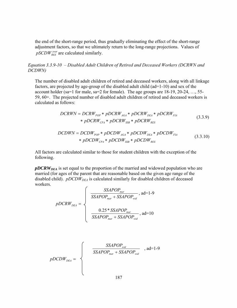
187

the end of the short-range period, thus gradually eliminating the effect of the short-range adjustment factors, so that we ultimately return to the long-range projections. Values of

yearRESpSCDW are calculated similarly.

Equation 3.3.9-10 – Disabled Adult Children of Retired and Deceased Workers (DCRWN and DCDWN)

The number of disabled adult children of retired and deceased workers, along with all linkage factors, are projected by age-group of the disabled adult child (ad=1-10) and sex of the account holder (sa=1 for male, sa=2 for female). The age groups are 18-19, 20-24, …, 55-59, 60+. The projected number of disabled adult children of retired and deceased workers is calculated as follows:

RESSSBCPA

FIADEAAGAPOP

pDCRWpDCRWpDCRWpDCRWpDCRWpDCRWDCRWDCRWN

∗∗∗∗∗∗=

(3.3.9)

RESSSBCPA

FIADEAAGAPOP

pDCDWpDCDWpDCDWpDCDWpDCDWpDCDWDCDWDCDWN

∗∗∗∗∗∗=

(3.3.10)

All factors are calculated similar to those for student children with the exception of the following. pDCRWDEA is set equal to the proportion of the married and widowed population who are married (for ages of the parent that are reasonable based on the given age range of the disabled child). pDCDWDEA is calculated similarly for disabled children of deceased workers.

widmar

mar

SSAPOPSSAPOPSSAPOP

+, ad=1-9

=DEApDCRW

widmar

mar

SSAPOPSSAPOPSSAPOP+

*25.0, ad=10

widmar

wid

SSAPOPSSAPOPSSAPOP

+ , ad=1-9

=DEApDCDW

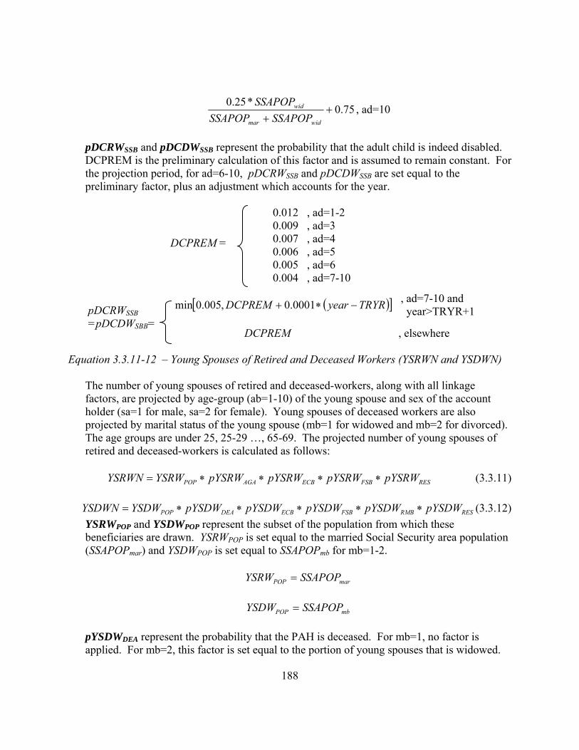
188

75.0*25.0

++ widmar

wid

SSAPOPSSAPOPSSAPOP

, ad=10

pDCRWSSB and pDCDWSSB represent the probability that the adult child is indeed disabled. DCPREM is the preliminary calculation of this factor and is assumed to remain constant. For the projection period, for ad=6-10, pDCRWSSB and pDCDWSSB are set equal to the preliminary factor, plus an adjustment which accounts for the year. 0.012 , ad=1-2 0.009 , ad=3 0.007 , ad=4 0.006 , ad=5 0.005 , ad=6 0.004 , ad=7-10

( )[ ]TRYRyearDCPREM −∗+ 0001.0,005.0min

DCPREM , elsewhere

Equation 3.3.11-12 – Young Spouses of Retired and Deceased Workers (YSRWN and YSDWN)

The number of young spouses of retired and deceased-workers, along with all linkage factors, are projected by age-group (ab=1-10) of the young spouse and sex of the account holder (sa=1 for male, sa=2 for female). Young spouses of deceased workers are also projected by marital status of the young spouse (mb=1 for widowed and mb=2 for divorced). The age groups are under 25, 25-29 …, 65-69. The projected number of young spouses of retired and deceased-workers is calculated as follows:

RESFSBECBAGAPOP pYSRWpYSRWpYSRWpYSRWYSRWYSRWN ∗∗∗∗= (3.3.11)

RESRMBFSBECBDEAPOP pYSDWpYSDWpYSDWpYSDWpYSDWYSDWYSDWN ∗∗∗∗∗= (3.3.12)

YSRWPOP and YSDWPOP represent the subset of the population from which these beneficiaries are drawn. YSRWPOP is set equal to the married Social Security area population (SSAPOPmar) and YSDWPOP is set equal to SSAPOPmb for mb=1-2.

marPOP SSAPOPYSRW =

mbPOP SSAPOPYSDW =

pYSDWDEA represent the probability that the PAH is deceased. For mb=1, no factor is applied. For mb=2, this factor is set equal to the portion of young spouses that is widowed.

DCPREM =

pDCRWSSB =pDCDWSBB=

, ad=7-10 and year>TRYR+1

189

1 , mb=1 (widowed)

marwid

wid

SSAPOPSSAPOPSSAPOP

+, mb=2 (divorced)

pYSRWAGA and represent the probability that the PAH is of the required age. pYSRWAGA is set equal to the portion of the married population who has an aged spouse (AGSP).

POPAGA YSRW

AGSPpYSRW =

pYSRWECB and pYSDWECB represent the probability that the young spouse has an entitled child in their care. pYSRWECB is set equal to the portion of persons meeting the previously mentioned requirements who have a minor or disabled adult child in their care. pYSDWECB ,by marital status, is set equal to the portion of persons meeting the previously mentioned requirements who have a minor or disabled adult child in their care. abMCRWN and

abDCRWN represent the total number of minor and disabled adult children of retired workers where the other parent (young spouse) is in the age bracket ab.

AGAPOT

ababab

ECB pYSRWYSRWDCRWNMCRWN

pYSRW∗

+=

( )

DEAPOP

totalAGA

totalDEA

totalPOP

mbAGA

mbDEA

mbPOPabab

mbECB pYSDWYSDW

pYSDWpYSDWYSDWpYSDWpYSDWYSDW

DCDWNMCDWNpYSDW

∗

⎥⎦

⎤⎢⎣

⎡∗∗∗∗

∗+

=

pYSRWFSB and pYSDWFSB represent the probability that the young spouse is not already receiving benefits based on another child in their care. This factor is set equal to one divided by the number of children in the average family (ASOFab) for the given age bracket of the spouse. For young spouses of retired workers, no factor is applied for sa=2.

abASOF

1 , sa=1

1 , sa=2

abFSB ASOF

pYSDW 1=

pYSDWDEA =

pYSRWFSB =

190

pYSDWRMB represents the probability that the spouse is not remarried. This factor is assumed to remain constant at 0.600.

600.0=RMBpYSDW pYSRWRES and pYSDWRES represent the probability that a person who is eligible to receive young-spouse benefits actually receive the benefits. For all historical years, year

RESpYSRW is calculated as the ratio of YSRWN, the actual number of young spouses of retired workers receiving benefits, to the number of persons meeting all previously mentioned requirements by age, sex, and marital status. year

RESpYSDW is calculated similarly, using the number of young spouses of deceased workers.

FSBECBAGAPOPRES pYSRWpYSRWpYSRWYSRW

YSRWNpYSRW∗∗∗

= , year<TRYR

RMBFSBECBDEAPOPRES pYSDWpYSDWpYSDWpYSDWYSDW

YSDWNpYSDW∗∗∗∗

= , year<TRYR

For each age, sex , and marital status, a least squares regression is used over the last ten years of historical data to determine a starting value in TR-1 for year

RESpYSRW . In addition, for each sex and marital status the regressed values of 1−TRYR

RESpYSRW are graduated over age using a weighted minimized third-difference formula to compute YSRWESTRES . YSRWESTRES are the preliminary estimates of 9+TRYR

RESpYSRW , the values in the tenth year of the projection period. For female young spouses, an adjustment, YSRWSRADJ , is applied to the tenth year of the projection period in order to match the projections made by the Short-Range office. The values of year

RESpYSRW for intermediate years are exponentially interpolated between 1−TRYR

RESpYSRW and 9+TRYRRESpYSRW (equal to YSRWYSRW SRADJESTRES ∗ ). After the 10th year

of the projection period, the adjustment factors are linearly graded to one over the 20 years beyond the end of the short-range period, thus gradually eliminating the effect of the short-range adjustment factors, so that we ultimately return to the long-range projections. Values of year

RESpYSDW are calculated similarly. Equation 3.3.13 – Number of Deaths of Insured Workers (LUMSUMab)

The number of deaths of insured workers is projected by sex and 5-year age group (ab=1-14). Age groups include 20-24, 25-29,…,80-84, 85+. EXPOSUREab, the estimated number of lump-sum payments paid during the year for age group ab, is calculated as the number of

191

total deaths during the year times the probability that the deceased was fully insured and has a surviving spouse or child. BASE is calculated as the ratio of the actual total amount of lump-sum death payments paid in TRYR-1 to the estimated total amount of lump-sum payments paid in TRYR-1. abLUMSUM is then calculated for each year in the projection period.

BASEEXPOSURELUMSUM abab ∗= (3.3.13) Appendix 3.3-1: Glossary AB: age group of the beneficiary AD: age of the disabled child AGSP: married population where at least one spouse is age 62 or older AM: age of the minor child ARFGT3: actuarial reduction factor for ages more than 3 years below normal retirement age ARFLE3: actuarial reduction factor for ages less than 3 years below normal retirement age AS: age of the student child ASDW: aged spouse of deceased worker by linkage factor, age (60-95+), sex of the account holder, marital status (widowed, divorced) and insured status (insured, uninsured). Linkage factors are:

POPASDW : population of potential aged spouse of retired workers

DEApASDW : probability that the primary account holder (PAH) is deceased

FIApASDW : probability that the PAH was fully insured at death

MBBpASDW : probability that the widow(er) is not receiving a young-spouse benefit for the care of a child

FIBpASDW : probability that the aged widow(er) is fully insured

GPBpASDW : probability that the aged-widow(er)'s benefits are not withheld or offset totally because of receipt of a significant government pension based on earnings in noncovered employment

RESpASDW : probability that a widow(er) eligible to receive his/her own retired-worker benefits would instead apply for and receive widow(er) benefits

ASDWN: final number of aged spouse of deceased workers (product of all linkage factors) ASOF: average number of children in a family, by age group (under 25, 25-29 …, 65-69) ASRW: aged spouse of retired worker by linkage factor, age (62-95+), sex of the account holder, and marital status of the beneficiary (married, divorced). Linkage factors are:

POPASRW : population of potential aged spouse of retired worker beneficiaries

DEApASRW : probability that the primary account holder (PAH) is not deceased

AGApASRW : probability that the PAH is of the required age

FIApASRW : probability that the PAH is fully insured

CPApASRW : probability that the PAH is receiving benefits

192

MBBpASRW : probability that the beneficiary is not receiving a young-spouse benefit

FIBpASRW : probability that the aged spouse is not fully insured

GPBpASRW : probability that the aged-spouse's benefits are not withheld because of receipt of a significant government pension based on earnings in noncovered employment

RESpASRW : probability that a person who is eligible to receive aged-spouse benefits actually receive the benefits

ASRWN: final number of aged spouse of retired workers (product of all linkage factors) AH: age of husband AW: age of wife BASE: ratio of actual to estimated total amount of lump-sum death payments paid in TRYR-1 CHI_62+: number of children having at least one parent aged 62 or older CHI_DEA: number of children having at least one deceased parent CON: number of persons converted from disabled-worker beneficiaries DCDW: disabled child of deceased workers by linkage factor, age group of the child (18-19, 20-24,..., 55-59, 60+) and sex of the account holder. Linkage factors are same as SCDW. POPDCDW : population of potential disabled children

AGApDCDW : probability that the PAH is age 62 or older

DEApDCDW : probability that the parent is either retired or deceased

FIApDCDW : probability that the PAH is fully insured

CPApDCDW : probability that the PAH is receiving benefits

SSBpDCDW : probability that the child is indeed disabled

RESpDCDW : probability that a child who is eligible to receive disabled-child benefits actually receive the benefits

DCDWN: final number of disabled children of deceased workers (product of all linkage factors) DCPREM: preliminary calculation of the probability that a child is disabled, by age DCRW: disabled child of retired workers by linkage factor, age group of the child (18-19, 20-24,..., 55-59, 60+) and sex of the account holder. Linkage factors are same as those for DCDW. DCRWN: final number of disabled children of retired workers (product of all linkage factors) DIB: number of disabled-worker beneficiaries DIFFADJ: adjustment which accounts for the difference between the actual and estimated prevalence rate at each age in the most recent historical years DISPREV: disability prevalence rate by age and sex DRC: delayed retirement credit DSDW: disabled spouse of deceased worker by linkage factor, age (50-69), sex of the account holder, and marital status (widowed, divorced). Linkage factors are:

POPDSDW : population of potential beneficiaries

DEApDSDW : probability that the primary account holder (PAH) is deceased

FIApDSDW : probability that the PAH was fully insured at death

193

SSBpDSDW : probability that the spouse is indeed disabled

DEBpDSDW : probability that the disabled spouse is not receiving another type of benefit

RESpDSDW : probability that a person who is eligible to receive disabled-spouse benefits actually receive the benefits

DSDWN: final number of disabled spouse of deceased workers (product of all linkage factors) ERROR: actual prevalence rate minus the regressed prevalence rate in the most recent historical year ESTPR: preliminary estimate of the prevalence rate for retired workers ESTPR2: secondary estimate of the prevalence rate for retired workers ESTRES: preliminary estimate of the RES factor for the tenth year of the projection period EXPOSURE: estimated number of lump-sum payments by age group (20-24, 25-29,…,80-84, 85+) FACTOR: adjustment for calculation of MBB factor of aged spouse of deceased worker FINS: portion of the SSA population that is fully insured FI_PAH: portion of married population where one spouse is fully insured FP: status of the parent (retired, deceased) GPOAGE: portion, by age, of the total beneficiaries expected to receive a significant government pension GPWHLD: total number of beneficiaries (for all ages) expected to receive a significant government pension IN: insured status of the beneficiary LFPR: labor force participation rates for age 62, by sex LUMSUM: number of deaths of insured workers by sex and age group (20-24,...,80-84,85+) MAR62PLUS: number of couples where both husband and wife are age 62 and over MS: marital status of the primary account holder MB: marital status of the beneficiary MBAPIA: ratio of the monthly benefit amount (MBA) to the primary insurance amount (PIA) by age (62-70) and sex MCDW: minor children of deceased workers by linkage factor, age of the child (0-17) and sex of the account holder. Linkage factors are:

POPMCDW : population of potential minor children

DEApMCDW : probability that the parent is either retired or deceased

FIApMCDW : probability that the PAH is fully insured

RESpMCDW : probability that a child who is eligible to receive minor-child benefits actually receive the benefits

MCDWN: final number of minor children of deceased workers (product of all linkage factors) MCRW: minor children of retired workers by linkage factor, age of the child (0-17) and sex of the account holder. MCRWN: final number of minor children of retired workers (product of all linkage factors) NRA: normal retirement age PAH: primary account holder REGPR: regressed prevalence rate for retired workers

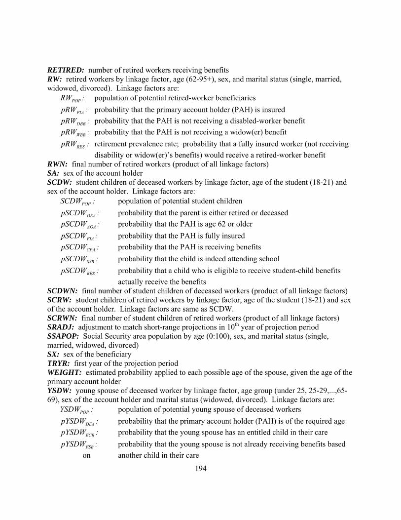
194

RETIRED: number of retired workers receiving benefits RW: retired workers by linkage factor, age (62-95+), sex, and marital status (single, married, widowed, divorced). Linkage factors are:

POPRW : population of potential retired-worker beneficiaries

FIApRW : probability that the primary account holder (PAH) is insured

DBBpRW : probability that the PAH is not receiving a disabled-worker benefit

WBBpRW : probability that the PAH is not receiving a widow(er) benefit

RESpRW : retirement prevalence rate; probability that a fully insured worker (not receiving disability or widow(er)’s benefits) would receive a retired-worker benefit

RWN: final number of retired workers (product of all linkage factors) SA: sex of the account holder SCDW: student children of deceased workers by linkage factor, age of the student (18-21) and sex of the account holder. Linkage factors are:

POPSCDW : population of potential student children

DEApSCDW : probability that the parent is either retired or deceased

AGApSCDW : probability that the PAH is age 62 or older

FIApSCDW : probability that the PAH is fully insured

CPApSCDW : probability that the PAH is receiving benefits

SSBpSCDW : probability that the child is indeed attending school

RESpSCDW : probability that a child who is eligible to receive student-child benefits actually receive the benefits

SCDWN: final number of student children of deceased workers (product of all linkage factors) SCRW: student children of retired workers by linkage factor, age of the student (18-21) and sex of the account holder. Linkage factors are same as SCDW. SCRWN: final number of student children of retired workers (product of all linkage factors) SRADJ: adjustment to match short-range projections in 10th year of projection period SSAPOP: Social Security area population by age (0:100), sex, and marital status (single, married, widowed, divorced) SX: sex of the beneficiary TRYR: first year of the projection period WEIGHT: estimated probability applied to each possible age of the spouse, given the age of the primary account holder YSDW: young spouse of deceased worker by linkage factor, age group (under 25, 25-29,...,65-69), sex of the account holder and marital status (widowed, divorced). Linkage factors are:

POPYSDW : population of potential young spouse of deceased workers

DEApYSDW : probability that the primary account holder (PAH) is of the required age

ECBpYSDW : probability that the young spouse has an entitled child in their care

FSBpYSDW : probability that the young spouse is not already receiving benefits based on another child in their care

195

pYSDWRMB : probability that the young spouse is not remarried RESpYSDW : probability that a person who is eligible to receive young-spouse benefits

actually receive the benefits YSDWN: final number of young spouse of deceased workers (product of all linkage factors) YSRW: young spouse of retired worker by linkage factor, age group (under 25, 25-29,...,65-69) and sex of the account holder. Linkage factors are:

POPYSRW : population of potential young spouse of retired workers

AGApYSRW : probability that the primary account holder (PAH) is of the required age

ECBpYSRW : probability that the young spouse has an entitled child in their care

FSBpYSRW : probability that the young spouse is not already receiving benefits based on another child in their care RESpYSRW : probability that a person who is eligible to receive young-spouse benefits

actually receive the benefits YSRWN: final number of young spouse of retired workers (product of all linkage factors)

196

Process 4:

Trust Fund

Operations & Actuarial Status

197

4. Trust Fund Operations and Actuarial Status

OCACT uses the Trust Fund Operations and Actuarial Status Process to project (1) the annual flow of income from payroll taxes, taxation of benefits, and interest on assets in the trust fund and (2) the annual flow of cost from benefit payments, administration of the program, and railroad interchange. The annual flows are projected for each year of the 75-year projection period. In addition, this subprocess produces annual and summarized values to help access the financial status of the Social Security program. The Trust Fund Operations and Actuarial Status Process is composed of three subprocesses: TAXATION OF BENEFITS, AWARDS, and COST. As a rough overview, TAXATION OF BENEFITS projects, for each year during the 75-year projection period, the amount of income from taxation of benefits as a percent of benefits paid. AWARDS projects information needed to determine the benefit levels of newly awarded retired workers and disabled workers by age and sex. COST uses information from the AWARDS and TAXATION OF BENEFITS subprocesses, as well as information from other processes, to project the annual flow of income and cost to the trust funds. In addition, COST produces annual and summarized measures of the financial status of the Social Security program. 4.1. TAXATION OF BENEFITS 4.1.a. Overview The 1983 Social Security Act specifies including up to 50 percent of the Social Security benefits to tax return filer’s adjustable gross income for tax liability if tax return filer’s adjusted gross income plus half of his (or her) Social Security benefits is above the specified income threshold amount of $25,000 as a single filer (or $32,000 as a joint filer). Moreover, the 1993 OBRA (Omnibus Budget Reconciliation Act) increased taxable benefits up to 85 percent if tax return filer’s adjusted gross income plus half of his (or her) Social Security benefits is above the specified income threshold amount of $34,000 as a single filer (or $44,000 as a joint filer). The proceeds from taxing up to 50 percent of the OASDI benefits, as a result of the 1983 Act, are credited to the OASI and DI Trust Funds, while additional taxes on the OASDI benefits, as a result of the 1993 Act, are credited to the HI Trust Fund. Income to the trust funds from such taxation is done by estimating ratios of taxes on benefits to benefits for the OASI and DI programs separately. These ratios, called “RTBs,” are applied to the projected OASI and DI benefit amounts to estimate tax revenues to the OASI, DI, and HI Trust Funds.

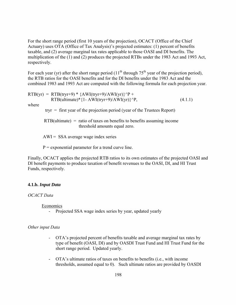
198

For the short range period (first 10 years of the projection), OCACT (Office of the Chief Actuary) uses OTA (Office of Tax Analysis)’s projected estimates: (1) percent of benefits taxable, and (2) average marginal tax rates applicable to those OASI and DI benefits. The multiplication of the (1) and (2) produces the projected RTBs under the 1983 Act and 1993 Act, respectively. For each year (yr) after the short range period (11th through 75th year of the projection period), the RTB ratios for the OASI benefits and for the DI benefits under the 1983 Act and the combined 1983 and 1993 Act are computed with the following formula for each projection year. RTB(yr) = RTB(tryr+9) * {AWI(tryr+9)/AWI(yr)}^P + RTB(ultimate)*{1- AWI(tryr+9)/AWI(yr)}^P, (4.1.1) where tryr = first year of the projection period (year of the Trustees Report) RTB(ultimate) = ratio of taxes on benefits to benefits assuming income threshold amounts equal zero. AWI = SSA average wage index series

P = exponential parameter for a trend curve line. Finally, OCACT applies the projected RTB ratios to its own estimates of the projected OASI and DI benefit payments to produce taxation of benefit revenues to the OASI, DI, and HI Trust Funds, respectively. 4.1.b. Input Data OCACT Data

Economics - Projected SSA wage index series by year, updated yearly

Other input Data

- OTA’s projected percent of benefits taxable and average marginal tax rates by

type of benefit (OASI, DI) and by OASDI Trust Fund and HI Trust Fund for the short range period. Updated yearly.

- OTA’s ultimate ratios of taxes on benefits to benefits (i.e., with income

thresholds, assumed equal to 0). Such ultimate ratios are provided by OASDI

199

Trust Fund and HI Trust Fund on a combined OASDI benefit type basis, and are expected to be updated periodically based on OTA’s update.

4.1.c. Development of Output For the short range period, OCACT uses OTA’s estimates of benefits taxable and average marginal tax rate projections for OASI and DI benefits, under the 1983 Act and 1993 Act, respectively. OCACT multiplies these two estimated ratios to compute the projected RTB ratios. After the short range period, formula 4.1.1 computes projected ratios of taxes on OASI benefits to OASI benefits and projected ratios of taxes on DI benefits to DI benefits under the 1983 Act (up to 50 percent of benefits taxable) and under the combined 1983 and 1993 Acts (up to 85 percent of benefits taxable). This formula essentially provides more weight to the ultimate RTB ratios as time progresses, using the ratio of AWI (10th year) to AWI (projection year) as the “weight.” Additionally, an exponential parameter P value to the AWI “weights” is set judgmentally such that the estimate continues the short range trend into the transitional 11th through 20th projection years before it approaches the ultimate RTB ratio. For the RTB ratios for up to 50 percent of benefits taxable, the P values were set at 0.98 and 0.99 to project smooth transitional RTB ratios for OASI and DI benefits, respectively.42 The ultimate RTB ratios used in the projection are based on OTA’s ultimate ratios, reduced by about 5 percent. The 5 percent reduction reflects estimates of the effect of the higher proportion of “old elderly” beneficiaries in the 2085 projected SSA (Social Security Area) population relative to the current SSA population distribution, due to improved mortality. For the 2008 Trustees Report, the ultimate RTB ratios for up to 50 percent of OASI and DI benefits taxable were set at 0.055 and 0.0275, respectively.43 Lastly, OCACT applies these projected RTB ratios to its own estimates of OASI and DI benefit payments to develop estimated taxation of benefit revenues to the OASI, DI, and HI Trust Funds, respectively.

42 For RTB ratios for up to 85 percent of benefits taxable, P values were set at .98 and .99 for OASI and DI benefits, respectively. 43 Ultimate ratios for up to 85 percent of OASI and DI benefits taxable, with the higher $34,000/$44,000 threshold amounts, were set at 0.092 and 0.046, respectively.

200

4.2. AWARDS Each year over 2 million workers begin receiving either retired-worker or disabled-worker benefits. The monthly benefits for these new awards are based on their primary insurance amount or simply PIA. The PIA is computed using the PIA benefit formula as specified in the 1977 amendments and the average indexed monthly earnings (AIME). The AIME depends on the number of computation years, Y, and the amount earned (earnings level) by a worker in each year. For retired-worker beneficiaries who have attained or will attain age 62 in 1991 or later, Y = 35. The AWARDS subprocess selects records from a 10% sample of newly entitled worker beneficiaries obtained from the Master Beneficiary Record (MBR).44 The selected sample, referred to as “sample”, contains 221,239 beneficiary records, and each record, r, includes a worker’s history of taxable earnings under the OASDI program as well as additional information such as sex, birth date, month of initial entitlement, and type of benefit awarded. To estimate the benefit levels of future newly awarded worker beneficiaries, the earnings records in the sample are modified to reflect the expected work histories and earnings levels of future beneficiaries (equation 4.2.1). After the modifications, an AIME is computed for each record in the future sample of beneficiaries (equation 4.2.2). Each AIME value is then subdivided into bend point subintervals45 (equation 4.2.3). As input to the Cost subprocess, the AIME values are used to calculate aggregate percentages of AIME in each bend point subinterval for each age at entitlement, sex and trust fund (equation 4.2.4). Equations 4.2.1 through 4.2.4 outline the overall structure and solution sequence. The subscript n refers to the bend point subinterval and r refers to the sample record. Projected Earnings = Projected Earnings (·) (4.2.1)

AIME(r) = 12

)(Earnings Indexed Highest ∗

∑Y

rY (4.2.2)

)(AIME rn = AIME n (·) (4.2.3)

PAPn = ∑

∑

rn

rn r

bp

)(AIME (4.2.4)

where bpn is the length of the nth bend point subinterval, 44 A record is selected if the year of initial entitlement equals 2004 and the beneficiary is in current pay status as of Dec. 2004, 2005 or 2006. Retired beneficiaries over age 70 and disability beneficiaries under age 20 or over age 64 were excluded. 45 The current law PIA formula has two bend points. For the purposes of PAP, the Awards subprocess instead uses 30 subintervals.

201

Y is the number of computation years, and AIMEn (r) is the AIME amount contained within the nth interval for record r. 4.2.b. Input Data Long-Range OCACT Projection Data

Demography– • Social Security area population by sex and age.

o From 1951 to 2085 o Updated annually

Economics – • Covered workers by sex and age--all.


• Covered workers by sex and age—with earnings posted to the Master Earnings File (MEF) only. - used with CWHS data to project future earnings levels


• Average Wage Index (AWI), projected values. o From 2007 to 2085 o Updated annually

• Average Taxable Earnings (ATE) —with earnings posted to the Master Earnings File (MEF) only. – used with CWHS data to project future earnings levels


• Projected Covered Worker Rate (for validation) o From 2007 to 2085 o Updated annually

• COLA (Cost Of Living Adjustment) o From 2007 to 2085 o Updated annually

• CPI (Consumer Price Index) o From 2007 to 2085 o Updated annually

Other input data

• 10% Awards Sample from the MBR and Master Earnings File o Newly awarded OASI / DI beneficiaries, whose initial entitlement year was

2004, are in current pay status as of Dec. 2004, 2005 or 2006. SSN Type of benefit

202

Type of claim (retirement or disability) Sex Date of birth Date of initial entitlement PIA amount Type of dual entitlement Dual entitlement status code PIFC LAF Trust fund Earnings histories for each worker from 1951 to 2003

o Generally updated annually, pending validation of the sample • Total taxable earnings and number of workers with taxable earnings by age, sex, and

year from the 2005 Continuous Work History Sample (CWHS). o From 1951 to 2005 o Updated annually

• AWI, Average Wage Index o From 1951 to 2006 o Data obtained from OCACT internet site. o Updated annually

• Wage base o From 1951 to 2008 o Data obtained from OCACT internet site. o Updated annually

• COLA, cost of living adjustment o From 1975 to 2007 o Data obtained from OCACT internet site. o Updated annually

• Amount of earnings needed to earn one quarter of coverage o From 1951 to 2008 o 1978-2008 data obtained from OCACT internet site. 1951-1977 values

estimated by applying projection methodology backwards from 1978. o Updated annually

4.2.c. Development of Output All equations described below are projected separately for the OASI and DI program. Equation 4.2.1 – Projected Earnings In order to estimate future benefit levels, the work histories and earnings levels in the current sample must be modified to represent those for a sample of worker beneficiaries who are newly

203

entitled in future years. There are three distinct modifications that must be made to the earnings records. For each future year, changes are made to the earnings records in order to reflect:

• Changes in Wage Bases. For some years, the projected wage base (contribution and benefit base), on an AWI discounted basis, is higher than the historical wage base. Therefore, the taxable earnings of future beneficiaries may need to include covered earnings above the reported historical wage base. Thus, for each record with reported taxable earnings at the wage base in a given year, AWARDS imputes his/her covered earnings.

• Changes in Covered Worker Rates.

Adjustments are made to work histories to be consistent with the projected changes in the economy-wide covered worker rates. Economy-wide covered worker rates are defined as the ratio of covered workers (from Economics subprocess) to the Social Security area population (from Demography subprocess).

• Earnings Experience in the CWHS46. Earning levels are modified to capture the changes to date that are reflected in the average taxable earnings reported in the CWHS by age and sex and the changes expected in the future.

Change in Wage Bases The earnings posted in the sample are limited by the historical wage base (contribution and benefit base). Prior to 1975, the maximum annual amount of earnings on which OASDI taxes were paid was determined by ad hoc legislation. After 1974, however, the annual maximum level was legislated to be determined automatically, based on the increase in the Social Security Average Wage Index (AWI). Prior to these automatic wage base increases, a relatively large portion of workers earned amounts above the base. Additional legislation raising the annual maximum taxable amount occurred in 1979, 1980, and 1981 to improve the financial future of the OASDI Trust Funds. In addition, the AWI used in the automatic calculation of the annual taxable maximum was modified in the early 1990s to include deferred compensation amounts. Therefore, for each record in the sample with earnings at the wage base, the AWARDS process imputes covered earnings above the historical wage base in order to reflect higher maximum taxable amounts imposed on future newly entitled beneficiaries. Please refer to appendix 4.2-2 at the end of this subprocess for details of this imputation. Change in Covered Worker Rates

46 This file is a 1% sample of individuals who had covered earnings at some point in their work histories.

204

The sample’s covered worker rate by age group and sex is defined as the ratio of (1) the number of those beneficiaries with covered earnings in the sample to (2) the total number of beneficiaries in the sample. For both males and females, the work histories are modified to reflect changes in the covered worker rates that would apply to a future sample of beneficiaries. These changes in the covered worker rates are based on changes in the economy-wide covered worker rates. The economy-wide covered worker rate is defined for an age-sex group in a particular period which represents a future sample cohort as the ratio of (1) the number of workers in the economy in this group that have some earnings in this period, to (2) the total midyear population in this group in this period. Economy-wide covered worker rates are calculated separately for each age-sex group and each historical and projected calendar year based on input data from the Economics and Demography subprocesses. In projecting sample covered worker rates, examination is done of the change in economy-wide covered worker rates, by age group, between the “base period” (representing individuals retiring in the sample year) and the “projection period” (representing individuals retiring in a year later than the sample year). Details of how this change is used to estimate the change in a covered worker rate for retired workers from a current period in the sample to a future period is given below for male and female, respectively. This presentation presumes that economy-wide covered rates increase over time, which is very common for females but not always true for males, based on 2008TR data. The calculation of the change in covered worker rate changes slightly if there is a reduction in relevant economy-wide covered worker rates. Example 1.1 gives an example of the calculations done for males if economy-wide covered worker rates decline. MALE

• The ratio of (1) the absolute difference in the economy-wide male covered worker rate between the two periods to (2) the potential difference in the economy-wide male worker rate in the sample year (i.e., 1 – economy-wide covered worker rate), multiplied by

• The corresponding potential difference in the sample’s male covered worker rates (i.e. 1 – sample male covered worker rate)).

FEMALE • The ratio of (1) the absolute difference in the economy-wide female covered

worker rate between the two periods to (2) the difference between the projected sample male covered worker rate and the economy-wide female worker rate in the sample year, is multiplied by

• The corresponding difference between the projected sample male covered worker rate and the sample female covered worker rate.

205

For additional explanation of this calculation, refer to example 1.1 and 1.2 in appendix 4.2-1 of this subprocess. Once the covered worker rates for the future sample of beneficiaries are determined, modifications to work histories of the sample to attain these rates are generally done by randomly removing or adding earnings. For males, the procedure is to select records randomly. However, for females, an additional selection criterion is included in order to achieve a distribution of the number of years of earnings for retired female beneficiaries. Female records with 10 or fewer years of earnings are not modified. A distribution limit is set for those female workers with 11 to 25 total years of career earnings within the projection year. This distributional limit changes each projected year. In the first year, the distribution limit for females is equal to the male distribution plus 97% of the difference between the initial male and female distributions within the sample. In each subsequent year, the percentage decreases by three percent until it reaches 0%. Thus, the females’ years of earnings distribution for those with 11 to 25 years of earnings is adjusted to approach that of the males. If a record is selected for adding earnings in a particular year, the amount of earnings added is based on the career earnings pattern of the selected record. When earnings are added to a record, AWARDS calculates the ratio of (1) the record’s Average Indexed Earnings, AIE47, to (2) the AIE of a hypothetical worker, w, whose year of birth and sex are the same as the record and whose annual earnings are set equal to average taxable earnings. For this purpose, average taxable earnings are determined by averaging the earnings over all records in the sample with the same sex and year of birth. Then, the amount of earnings48 in year t that is added to the record is Earnings(r, t) = PreATEf (sex, t) * (AIE (r) / AIE (w)),

where PreATEf(sex, t) is the average taxable earnings in year t, for those in the sample with the same sex as that of the record and calculated using projected earnings adjusted to reflect wage base changes for those retiring in year f.

For additional explanation of this calculation, refer to example 2 in appendix 4.2-1 of this subprocess. Earnings Experience in the CWHS

47 AIE is the average indexed annual earnings, average over the highest Y years of earnings (similar to AIME, but an annual amount). 48 In this subprocess, earnings histories of projected beneficiaries are all reflected as wage-indexed earnings histories in the 2004 sample.

206

For historical years beginning with 1951, the AWARDS subprocess uses average taxable earnings by age and sex (CWHSATEas) and numbers of covered workers by age and sex (CWHSCWas) as tabulated from the most recent CWHS file49. The AWARDS subprocess then projects these values from the base year (the last historical year in the CWHS file). Projections are made for each year after the base year through the end of the 75-year projection period using projected economy-wide number of covered workers by age and sex and annual average taxable earnings (ATE) from the Economics process50. The numbers of covered workers by age and sex (CWHSCWas) are projected by applying the annual growth rates by age and sex in the numbers of economy-wide covered workers50 produced by the Economics subprocess. In addition, CWHSATEas are projected. The first step is to determine preliminary CWHSATE'as by using the annual growth rate in the total economy-wide ATE50. A further multiplicative adjustment is made to each CWHSATE'as such that the resulting aggregate average taxable earnings, determined by combining the projected values of CWHSCWas and CWHSATEas for the year, produces the same growth rate as the growth in total taxable earnings from the Economic process. For additional explanation of this calculation, refer to example 3 in appendix 4.2-1 of this subprocess. The CWHSATEas are then used to change the earnings histories of the sample of newly entitled beneficiaries so that the earnings represent newly entitled beneficiaries in future years. The historical and projected CWHSATEas will be different from the corresponding average taxable earnings of a sample of new entitled workers beneficiaries. This is mainly because the CWHS contains earnings for workers who never become entitled to benefits. Thus, the CWHSATEas are used to distribute average taxable earnings among age-sex groups of future samples of new beneficiaries. For a given sex and age-group, the expected annual average taxable earnings of a future sample is denoted as ATEf'. ATEf' is computed by using the comparable changes51 in the CWHSATEas. In addition, the annual average taxable earnings of the sample (after adjustments to the records’ earnings levels for changes in wage bases and covered worker rates) are computed by sex and age-group and denoted as ATEf. The difference between these values is the amount by which the average annual earnings levels are adjusted. Let

ff ATE 'ATE) −=δ(t ,

49 These historical values are tabulated by the Economic subprocess. 50 These values are based on earnings posted to the Master Earnings File (MEF), excluding earnings posted to the suspense file. 51 The comparable changes reflect the wage-indexed changes in the CWHS ATEas between the year of earnings in the sample of new beneficiaries and the year of earnings in the projected sample.

207

for each year t. Then, (δ(t) * TotalWorkers(t)) is the total amount of earnings which the model distributes for a given sex and age-group in a way so that the average taxable earnings after distribution is ATEf'. For additional explanation of the calculation δ(t), refer to example 4 in the appendix of this subprocess. When δ(t) is negative, earnings for the year are decreased. To achieve ATEf' for the given sex and age-group, AWARDS multiplies CoveredEarnings(r, t) by a ratio,

αδ++=

)(ATE)(1)(ratio

f ttt .

The term, α, is an additional adjustment necessary because covered earnings above the wage base, have either no effect or only a partial effect on modifying ATEf to ATEf'. In the 2008 Trustees Report, α was set equal to -0.06 for both sexes and trust funds (OASI and DI). When δ(t) is positive, earnings for the year are increased. However, the method of increasing earnings differs between disabled beneficiaries (DIBs) and retired worker beneficiaries (OABs). For DIBs, this is done similar to the adjustment when δ(t) is negative, where the ratio is multiplied by covered earnings to raise each record’s earnings for year t. If the resulting value exceeds the future wage base in year t, taxable earnings would equal the wage base. Hence, again, a constant α is added to account for the fact that increasing covered earnings which are greater or equal to the future wage base has no effect and covered earnings a little below the future wage base has only a partial effect on modifying ATEf'' to ATEf

. For the 2008 Trustees Report, α = 0.02 for females and α = 0.03 for males. However, when earnings for the year are increased for OABs, the ratio takes into account that among OABs, there are many more workers with earnings near or above the future wage base. In order to account for this, AWARDS first computes z, such that

∑

∑∑

=

==⎟⎟

⎠

⎞

⎜⎜

⎝

⎛∗+⎟

⎟⎠

⎞⎜⎜⎝

⎛∗

=20

1

20

jn

20

1n

),ers(NumberWork

2)(

*),ers(NumberWork)()(

),ers(NumberWork)(

)(

n

tn

ttn

tht

tnt

tz

δδδ

,

where

208

(1) NumberWorkers(n, t) equals the number of workers whose earnings in year t fall within the nth interval, that is the number of workers whose earnings are greater or equal to IntervalLength (t)*(n-1) and less than IntervalLength (t)*n. For this calculation,

20)WageBase(t)(ngthIntervalLe =t . Also, TotalWorkers(t) = ∑

=

20

1

),ers(NumberWorkn

tn .

(2) j(t) is the interval, such that ⎥⎦

⎥⎢⎣

⎢−=

)ngth(IntervalLe)(20

ttj(t) δ .

(3) h(t) is the dollar amount from interval j(t) to the wage base,

))(-(21(t)ghtIntervaLen)( tjth ∗= .

Now the covered earnings of OAB records are multiplied by the ratio

α++=)(ATE

z(t)1ratio(t)f t

,

where α =0.03 for males and α = 0.02 for females. As AWARDS applies ratio(t) to Earnings(r, t) by each record, it makes sure total adjustment in a year does not exceed δ(t)*TotalWorkers(t). For additional explanation of this calculation, refer to example 5 in appendix 4.2-1 of this subprocess. Equation 4.2.2 – Average Indexed Monthly Earnings (AIME)

Step 1: Index Earnings To compute an individual’s AIME, all taxable earnings after 1950 are considered. First, the earnings are indexed up to the index year, i, which is defined as the year of attaining age 60 for retired-worker beneficiaries (eligible for benefits at age 62). For disabled-worker beneficiaries, i generally equals 2 years before the year of disability onset when disability insured. Thus,

⎪⎩

⎪⎨⎧

≥

<∗=

i

ititr

tif t),,Earnings(r

tif ,)( eAverageWag)( eAverageWag),Earnings(

t)nings(r,IndexedEar

Step 2: Determine Computation Years

209

For each record, the number of computation years, Y, is determined. For a retired-worker beneficiary in the sample, Y is 35. For a disabled-worker beneficiary, Y is calculated as follows: • Determine the number of elapsed years, which is equal to the year of disability onset (not

later than the year the worker turned age 62) minus the greater of either the year the disabled worker turned age 22 or 1951.

{ } { }22 age attainedYear ,1951max62 age attainedYear onset, disability ofYear minYears Elapsed −=

• Divide the elapsed years by five and truncate. Subtract this number (cannot exceed five) from the number of elapsed years.

• Y must be at least 2.

Step 3: Determine AIME Finally, an individual’s AIME is computed by summing the highest Y indexed earnings and dividing by the number of months in those years. Hence, for each record,

12Y(r) Earnings Indexed YHighest

AIME(r)∗

= ∑ .

Equation 4.2.3 – AIMEn(r) The Possible AIME value is divided into 30 intervals (bend point subintervals). The length of each interval in 1979 dollars is given below: $45, if 0 < n ≤ 13 bpn = $100, if 14 ≤ n ≤ 18 $200, if 19 ≤ n ≤ 28 $1000, if 29 ≤ n ≤ 30

Thus, the interval points of AIME division given below in 1979 dollars, yk, are equal to ∑=

k

nn

1

bp

and

⎭⎬⎫

⎩⎨⎧

⎥⎦⎥

⎢⎣⎢−= 5,

5rsElapsedYeaminearsY ElapsedY

210

$180, if k = 4 yk = $1085, if k = 18 $5085, if k = 30. For each record (r), the values for bpn are indexed from 1977 to his/her indexing year i using the Social Security average wage index (AWI). So for n = 1 to 30,

)1977(AWI(i) AWIbp)(bp ∗= nn r

Next the record’s AIME amount, AIME (r), is compared to the indexed intervals. If

∑−

=

1

1

)(bp k

nn r < AIME (r) ≤ ∑

=

k

1n

)(bp rn ,

then AIME (r) falls within the kth interval. And for n = 1 to 30, )(bp rn , if n < k

AIMEn (r) = AIME (r) - ∑=

k

nn r

1

)(bp , if n = k

0, if n > k

Equation 4.2.4 – Potential AIME Percentages (PAPS) Finally, for n = 1 to 30, AWARDS sums the values of AIMEn and bpn across all the records by sex, age, and trust fund. The ratio of these values gives the average potential AIME percentages

PAPn = )(bp

)(AIME

rn

rn

r

r

∑∑

.

211

Appendix 4.2-1 This appendix provides examples to help understand the calculations described in the model documentation of the AWARDS subprocess. These examples do not reflect actual values. Example 1.1: (OASI-Male) Task: In projecting the 2004 sample of newly entitled male beneficiaries to represent newly entitled male beneficiaries in 2050, an adjustment to the earnings histories for those males age 40-44 is needed to reflect lower covered worker rates expected for males in this age group. This example illustrates the calculation of the projected covered worker rate for males who are age 40-44 in the projection period. We will be comparing the group of males age 40-44 in the base period with its counterpart group of males age 40-44 in the projection period. Information given:

• Newly entitled retired male beneficiaries represented in the 2004 sample are age 40-44 in the base period, 1974-1986, and the counterpart group of males retiring in 2050 is age 40-44 in the projection period, 2020-2032.

• Based on the 2004 sample, covered worker rates for males age 40-44 in the base period = 88.0%.

• Economy-wide covered worker rate for males age 40-44 = 85.0% in the base period.

• Economy-wide covered worker rate for males age 40-44 = 75.0% in the projection period.

Calculations:

1. The potential difference in the economy-wide covered worker rate for

males age 40-44 in the projection period is 100.0% - 75.0% or 25.0%. 2. The potential difference in the economy-wide covered worker rate for

males age 40-44 in the base period is 100.0% - 85.0% or 15.0%. 3. The ratio from steps 1 and 2 is 25/15 or 166 2/3 %. 4. The potential difference in the sample’s covered worker rate for the males

age 40-44 in the base period is 100.0% - 88.0% or 12.0%. 5. The ratio from step 3 is multiplied by the potential difference in the

sample’s covered worker rate for males age 40-44 in the base period to yield 20.0% (166 2/3 % * 12.0% = 20.0% ).

6. The amount in step 5 (20.0%) would be subtracted from 100% to yield the sample covered worker rate for males who are age 40-44 in the projection period (80.0%).

212

Example 1.2 : (OASI - Female ) Task: In projecting the 2004 sample of newly entitled female beneficiaries to represent newly entitled female beneficiaries in 2050, an adjustment to the earnings histories for those females age 40-44 is needed to reflect higher covered worker rates expected for females in this age group. This example illustrates the calculation of the projected covered worker rate for females who are age 40-44 in the projection period. We will be comparing the group of females age 40-44 in the base period with its counterpart group of females age 40-44 in the projection period. Information given:

• Newly entitled retired female beneficiaries represented in the 2004 sample are age 40-44 in the base period, 1974-1986, and the counterpart group of females retiring in 2050 is age 40-44 in the projection period, 2020-2032.

• Based on the 2004 sample, covered worker rates for females age 40-44 in the base period = 75.0%.

• Economy-wide covered worker rate for females age 40-44 = 68.0% in the base period.

• Economy-wide covered worker rate for females age 40-44 = 72.0% in the projection period.

• Projected sample covered worker rate for males age 40-44 = 80.0% in the projection period. (as shown in example 1.1 above)

Calculations:

1. The absolute difference in the economy-wide covered worker rate for

females age 40-44 from the base period to the projection period is 72.0% - 68.0% or 4.0%.

2. The difference between the projected covered worker rate for males age 40-44 and the economy-wide covered worker rate for females age 40-44 in the base period is 80.0% - 68.0% or 12.0%.

3. The ratio from steps 1 and 2 is 4.0/12.0 or 33 1/3 %. 4. The difference between projected covered worker rate for males age 40-44

and sample’s covered worker rate for the females age 40-44 in the base period is 80.0%-75.0% or 5.0%.

5. The ratio from step 3 is multiplied by the potential difference in the sample’s covered worker rate for females age 40-44 in the base period to yield 1.667% (33 1/3 % * 5.0% = 1.667% ).

213

6. The amount in step 5 (1.667%) would be added to the sample covered worker rate for females age 40-44 in the base period (75.0%) to yield the projected covered worker rate for females who are age 40-44 in the projection period (76.667%).

Example 2: Task: In projecting the 2004 sample of newly entitled male OASI beneficiaries to represent newly entitled male OASI beneficiaries in 2021, an adjustment to the earnings histories for those males age 40-44 is needed to reflect higher covered worker rates expected for males in this age group. The amount of increase in the covered worker rates is computed as described in example 1 and found to be 4 percent. To achieve this target, the desired number of records with zero reported earnings in this age group are randomly selected and assigned earnings. This example illustrates the calculation of earnings to be assigned to a randomly chosen newly entitled retired male record with zero taxable earnings in the base year. Information given:

• Newly entitled retired male beneficiaries represented in the 2004 sample are age 40-44 in the base period, 1974-1986, and the counterpart group of males retiring in 2021 will be age 40-44 in the projection period, 1991-2003.

• Based on the 2004 sample, a male record, r = 60,000 has been randomly selected to replace his zero taxable earnings reported in the base year 1981 with an amount based on his career earnings pattern. This record is age 63 in 2004, and his year of birth is 1941.

• A beneficiary retiring at age 63 in 2021 will have a year of birth of 1958. And the corresponding projection year to the base year of 1981 is the projection year 1998.

• The Average Indexed Earnings for this record, AIE (60,000), is computed to be $43,465. Note: This value is calculated by (1) using the record’s annual taxable earnings reported each year through 2003, (2) converting them to 2003 year dollars, and then (3) summing the highest 35 years of earnings and dividing by 35.

• The Average Indexed Earnings for a hypothetical worker, AIE(w) whose year of birth is 1941 is $41,995. This value is calculated as above given the hypothetical worker earned the average taxable earnings in each of the base years for males retiring at age 63 in the 2004 sample.

214

• The projected Average Taxable Earnings52 of males retiring in 2021 for the projection year 1998 (converted to 1981 dollars53) is ATE2020(male,1998) = $18,718.

Calculations:

1. The ratio of the Average Indexed Earnings for record number 60,000,

AIE(60,000) to the Average Indexed Earnings of a hypothetical male worker born in 1941 and retiring at age 63, AIE(w) is $43,465/$41,995 or 1.035.

2. The amount in step 1 (1.035) would be multiplied to ATE2021(male,1998) given to be $18,718. This yields the amount of earnings assigned to record number 60,000 in the projection year 1998 representing a sample retiring in 2021, Thus, Earnings(60,000,1998) = 1.035 * $18,718 which equals $19,373.

Example 3: Task: The AWARDS subprocess estimates projected values of Average Taxable Earnings by age and sex using the values54 in the 2005 CWHS file supplied by the Economic subprocess as the base year on which to build our projections. This example illustrates the calculation of the projected Average Taxable Earnings of the CWHS in 2006 for 42 year old females, CWHSATE42,female(2006). We will be using the number of female covered workers age 42 and the total taxable earnings for females age 42 as given the in 2005 CWHS data. Information given:

• The total number of female covered workers age 42 in 2005 reported in the CWHS, CWHSCW42,female(2005) is 17,917. .

• The total taxable earnings for females age 42 in 2005 reported in the CWHS is $527,676,622.

• The economy-wide number of covered workers for females age 42 in 2005 is 1,782,357.

52 The average taxable earnings have been computed using projected earnings adjusted for changes in the wage base. Adjustments to earnings for changes in covered worker rates and the earnings experience in the CWHS have not been applied at this stage in the process. 53 All projection year dollars are converted back to ‘sample year’ dollar amounts. 54 Because not all earnings are posted for the most recent years for a given CWHS file, adjustment factors, based on historical trends, are applied by the Economic subprocess to complete these earnings. For the 2005 CWHS, adjustment factors were applied to data in years 2002 through 2005.

215

• The economy-wide number of covered workers for females age 42 in 2006 is 1,745,831.

• The economy-wide Average Taxable Earnings (ATE) in 2005 is $29,776. • The economy-wide ATE in 2006 is $31,078.

Calculations:

1. The growth in the economy-wide covered workers for females age 42

from 2005 to 2006 is 1,745,831/1,782,357 or 0.9795. 2. The growth rate in the economy-wide covered workers for females age 42

from step 1 is applied to the CWHS female covered workers age 42 in 2005, CWHSCW42,female(2005) to yield the projected covered workers for females who are age 42 in 2006, CWHSCW42,female(2006), 0.9795*17,917 or 17,550

3. The CWHS Average Taxable Earnings for females age 42 in 2005, CWHSATE42,female(2005) is computed using the given CWHS total taxable earnings and total covered workers for females age 42 in 2005 ($524,676,622 / 17,917 = $29,284).

4. The economy-wide growth rate in the average taxable earnings from 2005 to 2006 is $31,078 / $29,776 or 1.044

5. The growth rate in step 4 (1.044) is applied to the amount in step3 ($29,284) to estimate the preliminary CWHS Average Taxable Earnings for females age 42 in 2006, CWHSATE’42,female(2006) = $30,573 (1.044*$29,284)

6. The value from step 5 ($30,573) is multiplied by the value in step 2 (17,550) to yield the preliminary CWHS projected total taxable earnings for females age 42 in 2006 ($536,556,150).

7. Note a final multiplicative adjustment is made to CWHSATE’42,female(2006) to obtain CWHSATE42,female(2006). This adjustment is made once the preliminary taxable earnings have been computed for each age and sex in 2006 in order to ensure the growth rate in the aggregate average taxable earnings between 2005 and 2006 matches the growth rate in the ATE from the Economic process.

Example 4: Task: In projecting the 2004 sample of newly entitled female beneficiaries to represent newly entitled female beneficiaries in 2050, the projected Average Taxable Earnings of females in the sample (ATEf)55 for year t = 2020 must be adjusted by an amount, δ(2020), to meet a targeted Average Taxable Earnings(ATEf'') for 2020.

55 The average taxable earnings have been computed using projected earnings adjusted for changes in the wage base and for changes in covered worker rates.

216

This example illustrates the calculation of δ(2020) for the female cohort retiring at ages 62 to 70 in the projection year 2050. The cohort is age 32 to 40 in the projection year 2020. The value δ(2020) is the dollar amount in which the average annual earnings levels are adjusted for females in this age-group in the year 2020 and retiring in 2050. We will be comparing this group of females age 32-40 in the projection 2020 year with its counterpart group of females age 32-40 in the base year 1974. Information given:

• A cohort of newly entitled retired female beneficiaries retiring at ages 62 to 70 represented in the 2004 sample are ages 32-40 in the base year, 1974, and the counterpart group of females retiring in 2050 are ages 32-40 in the projection year, 2020.

• Based on the 2004 sample, the average taxable earnings for females in the base year 1974 is $4,536.

• For a sample projected to be retiring in 2050, the average taxable earnings (ATEf) for females in the projection year 2020 is $4,56456.

• Based on the 2005 CWHS data, the average taxable earnings for females ages 32-40 in the base year 1974 is $4,218.

• The projected average taxable earnings in the CWHS for females ages 32-40 in the projection year 2020 (in 1974 dollar amounts) is $4,640.

Calculations:

1. The increase in the average taxable earnings for females ages 32-40 in the

CWHS from the base year 1974 ($4,218) to the projection year 2020 ($4,640)12 is 10 percent.

2. Based on the value from step 1 the expected annual average taxable earnings (ATEf'') of females ages 32-40 in 2020 and retiring in 2050 is $4,536*1.10 or $4,990

3. The difference in ATEf'' ($4,990) and ATEf' ($4,564) yields the δ(2020) value $426 ($4,990 - $4,564 = $426).

Example 5: Task: In projecting the 2004 sample of newly entitled female beneficiaries to represent newly entitled female beneficiaries in 2033, for year t = 2023, δ(2023) is positive indicating an adjustment to earnings histories is needed to reflect higher average taxable earnings by this cohort for the projection year 2023.

56 Amount is in 1974 dollars, ‘sample year dollars’.

217

This example illustrates the calculation of the ratio(2023) in projection year 2023 for the female cohort retiring at ages 62 to 70 in the projection year 2033. The value, ratio(2023), is the adjustment ratio that will be applied to this cohort projected covered earnings in 2023 in order to achieve the targeted Average Taxable Earnings of this cohort for 2023. Information given:

• Earnings in the projection year 2023 for a group of newly entitled female beneficiaries retiring in 2033 is the counterpart corresponding to earnings in the base year 1994 for the group of newly entitled female beneficiaries in the 2004 sample.

• For newly entitled females retiring in 2033, the average taxable earnings (ATE2023) for the projection year 2023 is $19,97057.

• δ(2023) , the difference in the targeted average taxable earnings ATE2023' and ATE2023, is given to be $1,590.

• The wage base for the projection year 2023 (in 1994 dollar amounts) is $57,600

• The number of females in the projected 2033 sample with earnings below the wage base in 2023 is 52,800.

• The dollar amounts below the wage base in 2023 are divided into 20 equal intervals, IntervalLength(2023), of $2,880 each.

• The number of females in the 2033 sample who in 2023 have earnings falling in the 20th interval (their earnings are between $54,720 and $57,600) is 465

• For female OABs the constant α when δ(t) is positive is 0.02. Calculations:

• The interval in which $56,010 (the wage base in 2023 minus δ(2023) or $57,600-$1,590) falls within is interval j(2023) and is found by rounding δ(2023)/ IntervalLength(2023) or ($1590/$2880) to the lowest integer and subtracting this value from 20. This yields interval 20.

• The dollar amount from interval 20 to the wage base is h(2023), and is $2,880*(21-20) or $2,880

• Using the equation given on page 7 yields,

( ) ( )

800,522590,1$*465

880,2$590,1$800,52590,1$

)2023(∗+∗

=z = $1,594

57 Amount is in 1994 dollars, ‘sample year dollars’.

218

Note, the value for z(2023) is higher than δ(2023) in order to adjust for those records above or close to the wage base.

• The ratio multiplied to the covered earnings in 2023 for females retiring in 2033 is 1 + ($1,594/$19,970) + 0.02, or 1.10.

219

Appendix 4.2-2

This appendix provides additional details on how the AWARDS process imputes covered earnings above the historical wage base. To do this, AWARDS first computes the cumulative distribution, F, of the workers in the sample by their earnings level. Each historical wage base is divided into 20 equal intervals, n, and each interval length in year t is

20)WageBase(t)(ngthIntervalLe =t .

The cumulative distribution F(n, t) is the proportion of workers whose earnings are less than IntervalLength(t)*n, for n = 1 to 20. Let NumberWorkers(n, t) be the number of workers whose earnings in year t fall within the nth interval, that is the earnings are greater or equal to IntervalLength (t)*(n-1) and less than IntervalLength (t)*n. Also, let TotalWorkers(t) be the total number of workers in the sample with earnings in year t. Then for any n, 1 ≤ n ≤ 20,

)( rsTotalWorke

),(ersNumberWork),( F 1

t

tmtn

n

m∑== .

Once F(n, t) is computed for n = 1 to 20, AWARDS extends the function for those who had earnings at the wage base. To extrapolate F past the historical base (define F(n, t) for n > 20), AWARDS groups the maximum earners in each year in the sample based on the number of years they had earnings at the wage base during the next four years (0, 1, 2, 3, 4). Under the assumption of uniform distribution within each group, AWARDS assigns an F(nr, t) value to each record with earnings at the tax maximum beginning with the group that has no other earnings at the tax maximum during the next four years and ending with the group that has maximum earnings in each of the next four years. Note that for these beneficiaries F(nr, t) > F(20,t). Once F(nr, t) is computed for these beneficiaries, values for F(n, t), where n>20 are estimated. To find F(n, t), where n>20, the log odds transformation is utilized. The odds ratio,

n,t)n,tn,t

F(-1)F( )T( = , where n < 20

is the ratio of (1) the proportion of beneficiaries with earnings levels below the nth interval to (2) the proportion of beneficiaries with earnings levels above the nth interval. Next, the natural logarithm of the odds ratio is computed, giving the log odds transformation,

220

[ ] ⎟⎟⎠

⎞⎜⎜⎝

⎛==

)F(-1)F(ln)T(ln )Y(

n,tn,tn,tn,t , where n < 20

Utilizing the most linear portion of the function at the upper values of n, AWARDS regresses Y on those values. The regression line of Y has the form

nn,t *)(Y 10 ββ += Finally, the amount of covered earnings of a record that has earnings at the taxable maximum is determined based on the F(nr, t) value assigned to the record. The F(nr, t) value for this record is used in the above equations to determine T(nr, t), Y(nr, t), and then nr, the non-integer value for n in the regression equation of Y above. Thus, if earnings(r, t) = wage base in year t then

= t)nings(r,CoveredEar ngth(t)IntervalLe∗rn + error58,

where nr is the record’s non-integer value for n in the regression equation of Y above. If earnings(r, t) < wage base in year t, then CoveredEarnings (r, t) = earnings(r, t) At this point, AWARDS defines the expected taxable earnings of a future sample as,

⎩⎨⎧

≥<

=(t) base wagefuture t)nings(r,CoveredEar (t), base wagefuture(t) base wagefuture t)nings(r,CoveredEar , t)nings(r,CoveredEar

),(Earnings tr

58 The difference between Y(20,t) and )20(Y ,t .

221

4.3. Cost 4.3.a. Overview The COST subprocess projects the trust fund operations for each year of the long-range 75 year period. The COST subprocess projects the income and cost for each trust fund (OASI and DI). The two components of non-interest income are tax contributions and taxation of benefits. The other component of income is interest earned on the trust fund assets. The three components of cost are scheduled benefits, administrative expenses, and the railroad interchange. Each of these components is projected for each trust fund (OASI and DI). The end-of-year assets is computed by taking the beginning-of-year assets (ASSETS), adding tax contributions (CONTRIB), taxation of benefits (TAXBEN), and interest income (INT), and subtracting scheduled benefits (BEN), administrative expenses (ADM), and the railroad interchange (RR). Equations 4.3.1 through 4.3.6 outline this overall structure and sequence. CONTRIB = CONTRIB(·) (4.3.1) BEN = BEN(·) (4.3.2) TAXBEN = TAXBEN(·) (4.3.3) ADM = ADM(·) (4.3.4) RR = RR(·) (4.3.5) INT = INT(·) (4.3.6)

EOY BOYASSETS ASSETS CONTRIB TAXBEN INT BEN ADM RR= + + + − − − The COST subprocess produces annual values which help assess the financial status of the OASI, DI, and combined funds. These include the annual income rate (ANN_INC_RT), annual cost rate (ANN_COST_RT), and trust fund ratio (TFR) as outlined below. ANN_INC_RT = ANN_INC_RT (·) (4.3.7) ANN_COST_RT = ANN_COST_RT (·) (4.3.8) TFR = TFR(·) (4.3.9) The COST subprocess also produces summarized values. These values are computed for the entire 75-year projection periods, as well as 25- and 50-year periods. These include the actuarial balance (ACT_BAL), unfunded obligation (UNF_OBL), summarized income rate (SUMM_INC_RT), summarized cost rate(SUMM_COST_RT), and closed group unfunded obligation (CLOSEDGRP_UNFOBL).

222

ACT_BAL = ACT_BAL(·) (4.3.10) UNF_OBL = UNF_OBL(·) (4.3.11) SUMM_INC_RT = SUMM_INC_RT(·) (4.3.12) SUMM_COST_RT = SUMM_COST_RT(·) (4.3.13) CLOSEDGRP_UNFOBL = CLOSEDGRP_UNFOBL(·) (4.3.14) The following notation is used throughout this documentation:

• ni represents the first year of the projection period-2008 for the 2008 TR • ni+74 represents the final year of the projection period-2082 for the 2008 TR • nf represents the last year the cost program will project-2085 for the 2008 TR • nim1 is equal to ni-1 • nim2 is equal to ni-2 • ns is equal to ni+9 • nbase, the year of the sample, is equal to 2004

4.3.b. Input Data Data received as input from the short-range office are presented first. Then data from long range and all other sources are identified separately for each equation. Short-range OCACT Data

• Estimates for the first ten years of the projection period for the first six equations mentioned above.

• Assets at the beginning of year ni. All of this information is updated annually. Long-range OCACT and other Data i. Equation 4.3.1 – Tax Contributions (CONTRIB)

Economics-Process 2 • Projected effective taxable payroll for years nim1 through nf, updated yearly

Other

• Projected employee/employer payroll tax rate, by trust fund and year, for years 1981 through nf, updated as needed (e.g., as required due to legislative changes)

ii. Equation 4.3.2 – Scheduled Benefits (BEN)

223

Demography-Process 1 • Projected number of married and divorced people in the Social Security area

population age 65 and above for beginning of years nim1 through 2101, updated yearly

Economics -Process 2 • Historical COLA for years 1975 through nim2, updated yearly • Historical CPI for years 1990 through nim1, updated yearly • Projected cost of living adjustment (COLA) for years nim1 through nf, updated yearly • Historical SSA average wage index for year nim2, updated yearly • Projected percent increases in the average wage index for years nim1 through nf,

updated yearly • Coefficients for five dual entitlement equations, updated as needed

Beneficiaries-Process 3

• Incurred but not reported (IBNR) DI beneficiary distribution by age, duration of disability (0 through 9 years and 10+ years) and sex, updated every few years (subprocess #3.2). The number of DI beneficiaries in current-payment status is equal to the number of currently entitled DI workers times the IBNR factor.

• Projected number of disabled workers in current-pay status by sex, age in current-pay, and duration of disability (0 through 9 and 10+) for years nim1 through nf, updated yearly from subprocess 3.2

• Projected number of retired worker beneficiaries in current-pay status by sex, age in current-pay, and age at entitlement for years nim1 through nf, updated yearly from subprocess 3.3

• Projected number of auxiliary beneficiaries (by benefit category) of retired-worker, deceased-worker, and disabled-worker beneficiaries for years nim1 through nf, updated yearly from subprocess 3.3

• Projected number of disability insurance beneficiaries who convert to retirement insurance status upon the attainment of normal retirement age by age in current pay, for years nim1 through nf, updated yearly from subprocess 3.3

Other

• Total (aggregate) PIA and MBA, not actuarially reduced, of DI male and female workers in current payment status, updated yearly from the 1-A Table Supplement

• Total (aggregate) PIA and MBA, actuarially reduced, of DI male and female workers in current payment status, updated yearly from the 1-A Table Supplement

• Cumulative distribution of AIME dollars for newly entitled retired-worker beneficiaries by age (62 through 70) and sex, for years nim1 through nf, updated yearly from subprocess 4.2

• Cumulative distribution of AIME dollars for newly entitled disabled-worker beneficiaries by age (20 through 64) and sex, for years nim1 through nf, updated

224

yearly from subprocess 4.2. Ages 15 through 19 are assumed to have the same distribution of dollars as does age 20. Ages 65 and 66 are assumed to have the same distribution of dollars as does age 64

• Age distribution of newly entitled retired-worker beneficiaries in the AIME awards sample by sex, updated in years that the sample changes, from subprocess 4.2

• Starting average PIA matrix for retired-worker benefits for the year nim1, by age at entitlement, age in current-pay and sex, updated yearly

• Starting average PIA matrix for disabled-worker benefits, for the year nim1, by age in current-pay, duration and sex, updated yearly

• Starting average PIA matrix for beneficiaries who convert from disabled worker to retirement worker status for the year nim1, by age in current-pay and sex, updated yearly

• Starting average MBA matrix for retired-worker benefits for the year nim1, by age at entitlement, age in current-pay and sex, updated yearly

• Benefit relationships between worker and auxiliary benefits (linkages) for the year nim1, for all benefit categories and worker account holders of both sexes, updated yearly from qlink.xls

• Retroactive payment loading factors for auxiliary beneficiary categories for all years, for all all benefit categories and worker account holders of both sexes, updated as needed

• Post entitlement factors by sex and duration, for years ni through ns, updated yearly • Historical AIME deviation, by sex for years 1995 through nim1, updated yearly

iii. Equation 4.3.3 – Taxation of Benefits

Trust Fund Operations and Actuarial Status • Taxation of benefits as a percentage of scheduled benefits by trust fund for years

nim1 through nf, updated yearly from subprocess #4.1

iv. Equation 4.3.4 – Administrative Expenses

Economics-Process 2 • Average wage indexes for years ni through nf, updated yearly • Ultimate value of productivity factor for the period ni through nf updated yearly


• Total number of beneficiaries in current-pay status by trust fund for years ni through nf, updated yearly

v. Equation 4.3.5 – Railroad Interchange

Economics-Process 2 • Number of covered workers in five year age groups, for years ni through nf, updated

225

yearly • Effective taxable payroll for years nim1 through nf, updated yearly • Increase in the average wage index for years nim1 through nf, updated yearly


• Total number of beneficiaries in current-pay status by trust fund for years nim1 through nf, updated yearly


• Taxation of benefits as a percent of the amount of benefits scheduled to be paid, by trust fund for years nim2 through nf, updated yearly

Other input data

• Nominal annual yield rate on the combined OASDI trust fund for years ni through nf, updated as the ultimate real interest rate and ultimate CPI are changed by the Trustees. Ratio of railroad retirement average benefit to OASI average benefit for the year nim1, updated yearly

• Ratio of railroad disability average benefit to DI average benefit for the year nim1, updated yearly

• Number of railroad beneficiaries (retirement and disability) for each of the two years nim2 and nim1, updated yearly

• Average taxable earnings in railroad employment for each of the two years nim2 and nim1, updated yearly

• Railroad taxable payroll for each of the two years nim2 and nim1, updated yearly vi. Equation 4.3.6 – Interest Income

Economics-Process 2 • Annual increase in the CPI for years ni through nf, updated yearly

Trustees assumptions

• Ultimate real interest rate, reviewed annually vii. Equations 4.3.7 through 4.3.13 – Annual Values and Summarized Values All inputs for equations 4.3.7 through 4.3.13 are estimated internally in the Cost program. viii. Equation 4.3.14 – Closed Group Unfunded Obligation

Demographics-Process 1 • Single year population and mortality rate data for years 1941 through 2100, updated

yearly • Population projections by single year of age, 75-99, from nim2 to 2100, updated

226

yearly

Economics-Process 2 • Historical and projected single-year COLA data and average wage indexing series

(AWI) data for years 1975 through 2085 (for COLA) and 1951 through 2085 (AWI), updated yearly

• Projected number of covered workers by single year of age 15-74 from year ni through nf, updated yearly

• Aggregate number of covered workers aged less than 15, and aged 75 and over, from years ni through nf, updated yearly


• Total projected disabled workers by age for years 2007 to 2085, updated yearly Other

• Total count of beneficiaries in 20 of the 28 beneficiary categories (excluding retired workers, disabled workers, aged spouses (married, divorced, and dually entitled excess), and aged widow(er)s (married, divorced, and dually entitled excess) from the December 2007 Master Beneficiary Record (MBR)59—updated yearly

• Total benefits paid in 20 of the 28 beneficiary categories (excluding retired workers, disabled workers, aged spouses (married, divorced, and dually entitled excess), and aged widow(er)s (married, divorced, and dually entitled excess) from the December 2007 MBR—updated yearly

• Consumer Price Index data from 1951-1974 from Bureau of Labor Statistics • Number of covered workers and average taxable earnings by single year of age 1-14

for years 1991-2004 from 1 percent Continuous Work History Sample (CWHS), updated yearly to include year ni-4

• Number of covered workers and average taxable earnings by single year of age 75-99 for years 1991-2004 from 1 percent CWHS, updated yearly to include year ni-4

• Distribution of assumed age differentials of wives compared to age of husbands—separate distributions used for aged spouse benefits and aged widow(er) benefits, respectively

4.3.c. Development of Output i. Equation 4.3.1 – Payroll Tax Contributions (CONTRIB)

59 For disabled adult children of deceased workers and lump-sum beneficiaries, data was extracted from a 1- percent sample of the December 2007 MBR, mainframe dataset ACT.TAPEL.CAN1207. For the other 18 auxiliary beneficiary categories, data was extracted from the 100 percent December 2007 MBR, mainframe dataset ACT.TAPEH.MBR100.D0712.CANSORT.

227

It would be natural to estimate the payroll tax contributions by trust fund by multiplying the applicable employer/employee tax rate by effective taxable payroll. However, tax contributions are reported on a cash basis. That is, tax contribution amounts are attributed to the year in which they are actually received by the trust funds, while taxable payroll is attributed to the year in which earnings are paid. In other words, the lag between the time the tax liability is incurred and when the taxes are actually collected must be reflected. If lag represents the proportion of incurred payroll taxes estimated to be received by the trust fund (tf) in year yr, then tax contributions (CONTRIB) are given by the formula

( , ) ( , ) ( )(1 ) ( , 1) ( 1)

CONTRIB tf yr lag tax rate tf yr payroll yrlag tax rate tf yr payroll yr

= × ×+ − × − × −

for .yr ns≥ The value of lag is estimated from the combined OASI and DI tax contributions estimated to be collected in the final year of the short-range period, ns, and is given by

( )

( )

2 2

1 12

1

( , ) ( , 1) ( 1)

( , ) ( ) ( , 1) ( 1)

tf tf

tf

CONTRIB tf ns taxrate tf ns payroll nslag

taxrate tf ns payroll ns taxrate tf ns payroll ns

= =

=

− − × −=

× − − × −

∑ ∑

∑.

For the first ten years of the long-range period, tax contributions are set equal to those provided by the short-range office. The same value of lag is used for all years, and both trust funds, thereafter. ii. Equation 4.3.2 – Scheduled Benefits (BEN) (1) Disabled-Worker Benefits

Disabled Worker Beneficiary Matrix

The number of disabled-worker beneficiaries for a given year and sex are provided from the subprocess 3.2. For each projection year, two matrices are provided – one for males and one for females. The structure of each matrix is as follows:

• 11 columns. The columns are indexed by duration of disability (0-9 and 10+). • 52 rows. These rows correspond to the age in current pay, ages 15 through 66.

The COST subprocess, however, only uses 10 durations (0-8 and 9+), and 47 ages (ages 20 through 66). This requires a manipulation of the matrix of DI beneficiaries in current-pay status from subprocess 3.2. For ages in current pay greater than or equal to 30, the duration 9 and 10+ columns of this matrix are added to give the total number of duration 9+

228

beneficiaries. For ages (ag) between 20 and 30 inclusive, the number of beneficiaries in current-pay aged ag and duration ag-20 is the value provided by the DISABILITY subprocess added to the number of people in current pay aged ag-j and duration ag-20 for j=1,..,5. (For example, the number of people aged 20 of duration 0 is combined with the number of people aged 15, 16, 17, 18 and 19 of duration 0; the number of people aged 21 of duration 1 is combined with the number of beneficiaries in current-payment status aged 16, 17, 18, 19, and 20 of duration 1, and so on. In other words, the five nonzero diagonal of the matrix provided by the DISABILITY subprocess is “combined with” the diagonal directly below it.)

Building the Average Benefit Matrix for Disabled Workers In each projection year, the COST subprocess produces an average benefit matrix for each sex. Each matrix is a 47 by 10 matrix whose entries are the average benefit amounts of disabled worker beneficiaries whose age in current pay is indexed by the rows (ages 20 through 66) and whose duration of disability is indexed by the columns (durations 0 through 8 and 9+). The 1 percent Master Beneficiary Record (1% MBR) extract is processed by a side model. The final product of the side model is two matrices of benefits, one for males and one for females, for nim1 (2007 for the 2008 TR). For a given year of the projection period, a new average benefit matrix is obtained by moving the average benefit matrix from the previous year one year forward. The next few paragraphs describe this procedure. In general, for each age in current-pay, the age and duration are incremented by 1 and the previous PIA amount is given a cost of living adjustment. In addition, the beneficiaries are given a workers compensation adjustment. For each duration 0,1,...,7,j = and 8+ and sex, let the workers compensation offset factor be denoted ( , , ).wkcomp yr sx dur We have, for durations 0 through 8, that

( , , , ) ( 1, , 1, 1) (1 ( ))(1 ( , , )).

avgmba yr sx ag dur avgmba yr sx ag dur COLA yrwkcomp yr sx dur

= − − − × +× +

A more careful explanation of the last factor, ( , , ),wkcomp yr sx dur is given later in this document. See the section titled Average PIAs and MBAs for Disabled-Worker Beneficiaries, below. To move duration 8 average benefits to duration 9+ average benefits, both average benefits are given a cost of living adjustment. The resulting duration 9+ average benefit is the weighted average of the adjusted duration 8 and 9+ average benefits, weighted by the numbers of beneficiaries in current-pay status for durations 8 and 9+ respectively. The only column that is not handled by this procedure is the duration 0 column. This column corresponds to newly entitled disabled-worker beneficiaries, and is handled below.

229

Average Benefits for Newly Entitled Disabled-Worker Beneficiaries

The potential AIME percentage values for newly entitled disabled-worker benefits (DPAPs) are obtained from the AWARDS subprocess. The two bendpoints of the PIA formula, BP1 and BP2, are indexed by the increase in the average wage index. In 1979 dollars, the values of BP1 and BP2 are $180 and $1,085 respectively. The AIME dollars between 0 and BP1 are divided into four intervals (each of length $45 in 1979 dollars). The AIME dollars between BP1 and BP2 are divided into fourteen intervals (nine of length $45 and five of length $100, in 1979 dollars). Twelve additional intervals are added beyond BP2 (ten of length $200 and two of length $1,000, in 1979 dollars). To determine the average PIA for newly entitled beneficiaries, the DPAP values for each of the thirty intervals of AIME dollars are multiplied by the dollar amounts attributable to each interval (the length of the interval) and by the associated PIA factors. The distribution of prior year disability onset and current year disability onset is taken into consideration. It is assumed that this distribution is 6 months for prior year disability onset and 6 months for current year disability onset. In the formulas below, j = 1 signifies prior year disability onset and j = 2 signifies current year disability onset. Let:

• ( max( 60,1 ))_ ( , , )( 2)j

avgwg yr ag jWage Idx sx ag yravgwg nbase

− − +=

− for j=1,2.

• 1

61

(1 ( 1)) (1 ( )) 64_ ( , )

(1 ( ( 61)) 64 66.ag

k

COLA yr COLA yr agCum COLA ag yr

COLA yr k ag=

+ − × + <⎧⎪= ⎨ + − − ≤ ≤⎪⎩

∏

2

62

1 ( ) 63_ ( , )

(1 ( ( 62)) 63 66.ag

k

COLA yr agCum COLA ag yr

COLA yr k ag=

+ <⎧⎪= ⎨ + − − ≤ ≤⎪⎩∏

• 6 1 ,12 2jw = = j=1,2.

• PIA_factori represent the PIA factor for interval i (equal to 0.90 for intervals i=1,4, 0.32 for intervals i=5,…,18, and 0.15 for intervals i=19,…,30).

• AIME_dollarsi represent the length of interval i, expressed in 1979 dollars. • dpapi (yr,sx,ag) represent the DPAP value for newly entitled disabled workers in

year yr whose sex is sx and age is ag. To take into account the workers compensation offset to disability benefits, administrative data is reviewed, from which a factor is developed and applied to the average award benefit. We now describe how this factor, 2 ( , )facm p yr sx is computed. The 1-A table supplement as of the end of December, 2007, contains total award PIA and MBA data for disabled workers,

230

by sex, for beneficiaries both non-actuarially reduced and actuarially reduced. Let _ _ ( , )totmba DIB nar yr sx and _ _ ( , )totpia DIB nar yr sx be the total MBA and PIA respectively

for DIBs that are not actuarially reduced as found in the 1-A table. In the historical period 1988-nim1 we define 2 ( , )facm p yr sx to be the ratio of the total MBA to the total PIA for those not actuarially reduced. In other words,

_ _ ( , )2 ( , ) ._ _ ( , )

totmba DIB nar yr sxfacm p yr sxtotmba DIB nar yr sx

=

In the period ni through ns+9, 2 ( , )facm p yr sx is defined as follows. Let

1/102 ( 1, )2 ( 1, ) .

2 ( 11, )facm p yr sxx facm p yr sxfacm p yr sx

⎛ ⎞−= − ×⎜ ⎟−⎝ ⎠

This value is further adjusted to reflect that one quarter of the offset amounts end within the first entitlement year (as suggested by data). As a result, for yr = ni, … , ns+9,

2 ( , ) (1 ) 0.250.25 0.75 .

facm p yr sx x xx

= + − ×= + ×

The factor reaches its ultimate value in years ns+10 and later.

The preliminary average PIA for newly entitled disabled worker beneficiaries may now be defined. It is equal to

30

1

2

1

_ ( , , ) _ _ ( , , )

_ ( , , ) _ ( , )

2 ( , ).

i i ii

j j jj

LR awdpia sx ag yr PIA factor AIME dollars dpap yr sx ag

w Wage Idx sx ag yr Cum COLA ag yr

facm p yr sx

=

=

= × ×

⎛ ⎞× × ×⎜ ⎟⎝ ⎠

×

∑

∑

The preliminary average PIA for newly entitled benefits is further adjusted by a factor, adjpia, designed to be the factor that adjusts the long-range projected newly entitled monthly benefit amount (MBA) to the value projected by short range in the short-range period. Therefore, for years in the short range period (yr = ni, … , ns),

( , , ) _ ( , , ) ( , ).awdpia sx ag yr LR awdpia sx ag yr adjpia sx yr= × Once these average PIAs of newly entitled disabled-worker beneficiaries are computed, their values are filled into the average PIA matrices for duration 0 for the appropriate entitlement age.

Average PIAs and MBAs for Disabled-Worker Beneficiaries An overall average PIA of newly entitled disabled worker beneficiaries for each sex and projection year is computed by taking the weighted average of awdpia(sx,ag,yr), the weights

231

being the number of disabled workers in current payment status of duration zero. This value is denoted awdpia(sx,yr). In addition, an overall average PIA and MBA for all disabled worker beneficiaries in current-payment status is computed by finding the weighted average of the average PIAs for each age in current-pay and duration with the number of people in current pay for each of these ages and durations. The average PIAs were already reduced by a workers compensation offset factor, as briefly described above; a more careful description is given in this section. To get the average MBAs, we apply a factor which reflects the differences in average MBAs and PIAs for disabled workers, isolating only the trend in cases with an actuarial reduction. We also provide a relatively small reduction to reflect offsets starting and stopping in the year of DI entitlement that are not captured by the current method. Workers Compensation Offset Factors For each duration 1,...,7,j = and 8+ and sex we define a workers compensation factor. This factor is applied to the average worker PIA matrix as mentioned above. It is denoted ( , , ).wkcomp yr sx dur Let 2 _ ( )facm p pct dur be defined as in the following table.

Duration Cumulative product above set at x% of way between original facm2p and 1

1 0.396162 2 0.577085 3 0.671787 4 0.732777 5 0.789194 6 0.819700 7 0.842675

8+ 0.866667 Then ( , , )wkcomp yr sx dur is defined so that

1

2 _ ( ) 2 ( , ) (1 ( , , )).dur

j

facm p pct dur facm p yr sx wkcomp yr sx j=

= × +∏

This is an iterative process which first computes ( , ,1)wkcomp yr sx by solving the above equation with dur set equal to 1. The remaining factors for higher durations are then computed recursively using the above formula. Trend in Average MBA to Average PIA

232

This trend is captured in a factor denoted 2 ( , ).Fam p yr sx The 1-A table supplement as of the end of December, 2007, contains total award PIA and MBA data for disabled workers, by sex, for beneficiaries both non-actuarially reduced and actuarially reduced. Let

_ ( , )totmba nar yr sx and _ ( , )totpia nar yr sx be the total MBA and PIA respectively for DIBs that are not actuarially reduced as found in the 1-A table. Similarly, let _ ( , )totmba ar yr sx and

_ ( , )totpia ar yr sx be the total MBA and PIA respectively for cases that are actuarially reduced. In the historical period 1988-nim1 we define 2 ( , )fam p yr sx to be the ratio of the total MBA to the total PIA for those not actuarially reduced. In other words,

_ ( , ) _ ( , )2 ( , ) ._ ( , ) _ ( , )

totmba ar yr sex totpia nar yr sexFam p yr sextotpia ar yr sex totpia nar yr sex

+=

+

In the period ni through ns+9, 2 ( , )facm p yr sx is defined by

1/102 ( 1, )2 ( , ) 2 ( 1, ) .

2 ( 11, )Fam p yr sxFam p yr sx Fam p yr sx

Fam p yr sx⎛ ⎞−

= − ×⎜ ⎟−⎝ ⎠

The factor reaches its ultimate value in years ns+10 and later. More Workers Compensation Offsets As mentioned above, we also we provide a relatively small reduction to reflect offsets starting and stopping in the year of DI entitlement that are not captured by the current method. Administrative data suggests that these factors should be

Duration Percentage Reduction 0 0.3400% 1 0.2020% 2 0.0664% 3 0.0336% 4 0.0121%

and 0 for higher durations. We define wkcomp_red(dur) to be 1 minus these percentage reductions. Computation of Average MBA for DI Workers The disabled worker PIA as presented in the average benefit matrix was already incremented by age and duration using a COLA and a workers compensation adjustment. The average PIA by year, age and duration, is denoted ( , , , ).avgpia yr ag sx dur The overall average MBA by year and sex is the weighted average of

( , , , ) _ ( ) 2 ( , , ),avgpia yr ag sx dur wkcomp red dur Fam p yr sx dur× × the weights being the number of DI workers in current payment status by age, sex, and duration.

DI Conversions

233

Disabled-worker beneficiaries convert to retired-worker beneficiary status (called DI conversions) at normal retirement age (NRA). The average DI conversion benefit for a given sex and single age 65 through NRA is the weighted average of the average DI conversion benefits for that sex and age, weighted by the number of people in current pay in each duration. Both the average conversion benefit for each sex and age 65 though NRA and the number of people in current pay for these ages are used in the computation of average retired worker benefits (see subsection (2) below).

(2) Retired-Worker Benefits

Retired-Worker Beneficiary Matrix The number of retired-worker beneficiaries for a given year and sex are provided from subprocess 3.3. Two matrices are provided – one for males and one for females. The structure of each matrix is as follows:

• 10 columns. The first 9 columns are the age at entitlement, ages 62 through 70. The last column is the number of disabled workers who are projected to convert to retired-worker beneficiary status (DI conversions) at normal retirement age.

• 34 rows. These rows correspond to the age in current pay, ages 62 through 94 and ages 95+.

Note that the entries on the diagonal (where age in current-pay equals age at entitlement) is the number of new entitlements projected for that year.

Building the Average Benefit Matrices for Retired Workers In each projection year, the COST subprocess produces four average benefit matrices. For each sex there are two matrices, an average monthly benefit amount (MBA) matrix and the average primary insurance amount (PIA) matrix. Each matrix has the same structure as the beneficiary matrices. In other words, each matrix is a 34 by 10 matrix whose entries are the average benefit amounts of retired worker beneficiaries whose age in current pay is indexed by the rows and whose original age at entitlement is indexed by the columns. The final column simply gives the average benefits for DI conversions at the various ages in current pay. The 1% MBR extract is processed by a side model. This side model computes a starting matrix for year ni-1. This starting matrix contains the four initial benefit matrices, constructed using the most recent data. For a given year of the projection period, the average benefit matrix is updated from its previous year’s value incrementing each benefit amount (PIA or MBA) by one year of age and increasing it by a cost of living adjustment (COLA). MBAs are increased by the appropriate post entitlement factor60 for males and females.

60 Post entitlement factors are used to reflect (a) the higher survival rates for those receiving higher benefits and (b)

234

Adjusted age 94 benefits and age 95+ benefits are averaged to get the new average benefit for age 95+. DI conversion benefits are handled similarly, except the average conversion benefit for each age 64 through 66 is combined (as a weighted average) between the DI conversion average benefits computed in subprocess 3.2 and the DI conversions of the corresponding age already receiving benefits (provided by subprocess 3.3). The entries along the diagonal, the average benefits of newly entitled beneficiaries by age, must still be computed. The remainder of this section will explain how these average benefits are computed. Once these are computed, all entries are computed and the average benefit matrix for the year is complete.

Average Benefits for Newly Entitled Retired Worker Beneficiaries

The potential AIME percentage (OPAPs) values for newly entitled retired-worker benefits are obtained from subprocess 4.2. The OPAPs for the projection of average benefits for newly entitled retired-worker beneficiaries are modified by the COST subprocess. The reason is that the age distribution of newly awarded retired worker beneficiaries as determined in the awards sample is used for each projection year, i.e., the age-sex distribution matches that of the sample. These new potential AIME percentages are denoted OPAP1. To incorporate the projected change in the age distribution of projected newly awarded retired-worker beneficiaries for the purpose of determining their average benefits, we use a “shuttling method.” Additional details about the shuttling method are given in Appendix 4.3-1.

Average benefits for newly eligible retired-worker beneficiaries are calculated by sex for single year ages 62 through 69, and ages 70+. The two bendpoints of the PIA formula, BP1 and BP2, are indexed by the increase in the average wage index. In 1979 dollars, the values of BP1 and BP2 are $180 and $1,085 respectively. The AIME dollars between 0 and BP1 are divided into four intervals (each of length $45 in 1979 dollars). The AIME dollars between BP1 and BP2 are divided into fourteen intervals (nine of length $45 and five of length $100, in 1979 dollars). Twelve additional intervals are added beyond BP2 (ten of length $200 and two of length $1,000, in 1979 dollars). To determine the average PIA for newly entitled beneficiaries, the OPAP1 values for each interval of AIME dollars is multiplied by the dollar amounts attributable to each interval (the length of the interval). More precisely, let

• PIA_factori be the PIA factor for subinterval i (equal to 0.90 for intervals i=1,4, 0.32 for intervals i=4,…,18, and 0.15 for intervals i=19,…,30), AIME_dollarsi be the length of subinterval i,

• opap1i (yr,sx,ag) be the modified PAP value for retired workers newly entitled in year yr whose sex is sx and whose age is ag.

earnings after retirement.

235

• ( ( 62))_ ( , )( 2)

avgwg yr agWage Idx ag yravgwg nbase

− −=

−

Then the average PIA for these newly entitled retired worker beneficiaries is equal to

30

1

_ ( , , )

_ _ ( , ) _ 1 ( , , ).i i ii

LR awdpia sx ag yr

PIA factor Wage Idx ag yr AIME dollars opap yr sx ag=

= × × ×∑

This formula incorporates the fact that the PAP values are the estimated cumulative distribution of AIME dollars. The average award MBA for a worker beneficiary is then the average award PIA multiplied by the appropriate actuarial reduction factors and delayed retirement credits, arfdrc(ag,yr). The average MBA for newly entitled benefits is also adjusted by a factor, adjpia, designed to be the factor that adjusts the long-range projected newly entitled MBA to the short-range projection in the short-range period. Therefore,

( , , ) _ ( , , ) ( , ) ( , ).awdmba sx ag yr LR awdpia sx ag yr adjpia sx yr arfdrc ag yr= × × Once these average benefits of newly entitled retired-worker beneficiaries are computed, their values are filled into the appropriate average benefit matrices. For summary purposes, the COST subprocess computes an average PIA and MBA for all male and female newly entitled retired-worker beneficiaries, as well as for all retired-worker beneficiaries in current-payment status. These are just the respective weighted averages of the average PIAs and MBAs by age and sex, the weights being the number of newly entitled retired-worker beneficiaries. These average PIAs and MBAs are adjusted in such a way so that their values, in the short-range period, match the projection provided by the short-range office. In a similar way, the COST subprocess computes an average PIA and MBA for male and female retired workers in current payment status, also as a weighted average.

(3) Annualizing Benefits Scheduled benefits are calculated by trust fund and projection year. For each year scheduled benefits for each trust fund are found by adding up the appropriate benefit categories. This section considers all benefit amounts except the “dual entitlement excess amount.” If a retired worker beneficiary is also entitled to spouse or widow(er) benefits and the auxiliary benefits are greater, than the amount by which the auxiliary benefit exceeds the worker’s MBA is the dual entitlement excess amount. The four categories of excess amounts (dually entitled wives, widows, husbands, and widowers) are projected separately. More information is found in subsection (4). The first step is to annualize benefits by category. The average benefit for a specific auxiliary beneficiary category (avgben) is found by multiplying the linkage factor (the assumed

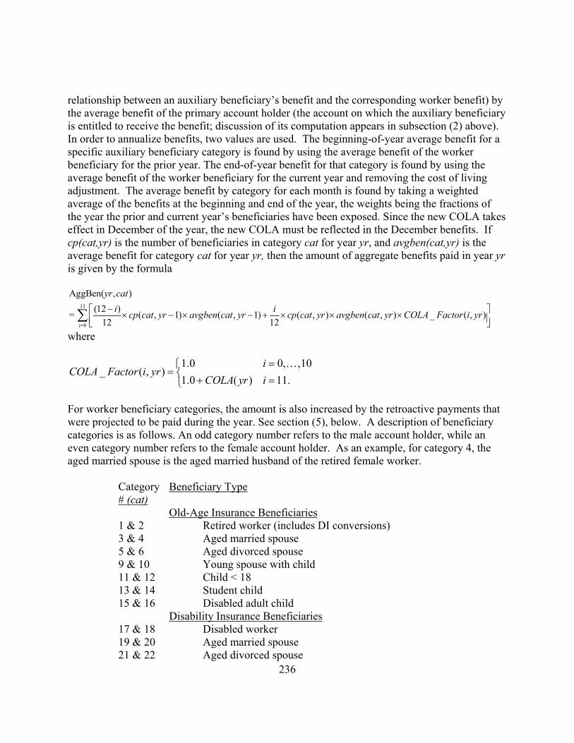
236

relationship between an auxiliary beneficiary’s benefit and the corresponding worker benefit) by the average benefit of the primary account holder (the account on which the auxiliary beneficiary is entitled to receive the benefit; discussion of its computation appears in subsection (2) above). In order to annualize benefits, two values are used. The beginning-of-year average benefit for a specific auxiliary beneficiary category is found by using the average benefit of the worker beneficiary for the prior year. The end-of-year benefit for that category is found by using the average benefit of the worker beneficiary for the current year and removing the cost of living adjustment. The average benefit by category for each month is found by taking a weighted average of the benefits at the beginning and end of the year, the weights being the fractions of the year the prior and current year’s beneficiaries have been exposed. Since the new COLA takes effect in December of the year, the new COLA must be reflected in the December benefits. If cp(cat,yr) is the number of beneficiaries in category cat for year yr, and avgben(cat,yr) is the average benefit for category cat for year yr, then the amount of aggregate benefits paid in year yr is given by the formula

11

i=0

AggBen( , ) (12 )= ( , 1) ( , 1) ( , ) ( , ) _ ( , )

12 12

yr cati icp cat yr avgben cat yr cp cat yr avgben cat yr COLA Factor i yr−⎡ ⎤× − × − + × × ×⎢ ⎥⎣ ⎦

∑

where

1.0 0, ,10_ ( , )

1.0 ( ) 11.i

COLA Factor i yrCOLA yr i

=⎧= ⎨ + =⎩

K

For worker beneficiary categories, the amount is also increased by the retroactive payments that were projected to be paid during the year. See section (5), below. A description of beneficiary categories is as follows. An odd category number refers to the male account holder, while an even category number refers to the female account holder. As an example, for category 4, the aged married spouse is the aged married husband of the retired female worker.

Category Beneficiary Type # (cat)

Old-Age Insurance Beneficiaries 1 & 2 Retired worker (includes DI conversions) 3 & 4 Aged married spouse 5 & 6 Aged divorced spouse 9 & 10 Young spouse with child 11 & 12 Child < 18 13 & 14 Student child 15 & 16 Disabled adult child

Disability Insurance Beneficiaries 17 & 18 Disabled worker 19 & 20 Aged married spouse 21 & 22 Aged divorced spouse

237

25 & 26 Young spouse with child 27 & 28 Young child 29 & 30 Student child 31 & 32 Disabled adult child

Survivors Insurance Beneficiaries 33 & 34 Aged married widow 35 & 36 Aged divorced widow 39 & 40 Young married disabled widow 41 & 42 Young divorced disabled widow 43 & 44 Aged parent 45 & 46 Young married widow with child 47 & 48 Young divorced widow with child 49 & 50 Young child 51 & 52 Student child 53 & 54 Disabled student child 55 & 56 Lump sum death benefit ($255)

(4) Dually Entitled Beneficiaries and Benefits

Number of Dually Entitled Beneficiaries There are four categories of dually entitled beneficiaries. They are the dually entitled wives (1), widows (2), widowers (3), and husbands (4). The number of dually entitled husbands is very small (currently less than 0.05% of all dually entitled beneficiaries and are expected to remain at this level in the future). As a result, the number of dually entitled husbands and their benefits are not projected. The equations used to project the number of dually entitled beneficiaries each have three terms. Each equation has three coefficients, ( ) ,k

ja 1, 2,3j = (corresponding to each of the categories above). These coefficients are provided by the Economics process based on historical series of the other terms in the equations. These terms contain the basic quantities (a) projected weighted average AIME deviations of newly entitled retired worker beneficiaries for each sex [AIME_Dev(yr,sx)] and (b) average PIA of newly entitled retired worker beneficiaries by sex, wage indexed to the year of the sample [PIA(yr,sx)]. Therefore, the three equations

( ) ( ) ( ) ( )1 2 3

AIME_Dev(yr,M) AIME_Dev(yr,F) PIA(yr,M) PIA(yr,F)PctExp ( )PIA(yr,M) PIA(yr,F) PIA(yr,M)

k k k kyr a a a −= + +

( 1,2,3k = ) project the percentage of the exposed population entitled to wife (1), widow (2), and widower (3) benefits. The table below shows the regression coefficients used in the 2008 Trustees report.

238

k Type ( )1

ka ( )2ka ( )

3ka 2R

1 Wife 0.04 0.05 0.55382 0.9223 2 Widow 0.15 0.16 0.41284 0.4797 3 Widower 0.03 0.02 -0.06570 0.7535

In the above equations, the average PIA of newly entitled beneficiaries by sex has already been computed (see subsection (2) above). The remaining paragraphs discuss the methodology used to compute the AIME deviations that are used in the above equation. This process requires two steps:

• obtain the AIME deviation in each year by sex and • obtain a 10 year historical average of these AIME deviations.

The projection of a deviation of AIME values [std_dev(yr,sx)] is as follows. The projection uses the interval of AIME dollars for 1979. The 1979 bend points are $180 and $1,085. The entire interval of AIME dollars is divided into 30 smaller intervals [as was done in the projection of average benefits of newly entitled beneficiaries; see subsection (2)]. The left endpoints of these intervals ($0, 45, 90, 135, 180, 280, 380, etc.) are the 1979 interval point values. These 1979 interval point values are wage indexed to the award sample year (2004 for the 2008 Trustees Report). Each interval point i, in 2004 wage indexed dollars, is

AverageWageIndex(2002)Interval Point = (1979 Interval Point ) .AverageWageIndex(1977)i i ×

Each interval point is assigned a probability using the OPAP1 values [see subsection (2)]. Each interval is assigned probability

1

1.0 1 ( , , ) 1( , , )

1 ( , , ) 1 ( , , ) 2, , 29.i

ii i

opap yr ag sx ip yr sx ag

opap yr ag sx opap yr ag sx i+

− =⎧= ⎨ − =⎩ K

The average AIME of each newly entitled beneficiary aged ag=62,…,70, by sex (sx) and projection year (yr) in sample year (2004) dollars is

10

1AvgAIME(yr,sx,ag)= ( , , ) Interval Point .i i

ip yr sx ag

=

×∑

The variance of AIME for each newly entitled beneficiary aged ag=62,…,70, by sex (sx) and projection year (yr) in sample year (2004) dollars is

[ ]30

2

1VarAIME(yr,sx,ag)= ( , , ) Interval Point AvgAIME(yr,sx,ag) .i i

ip yr sx ag

=

× −∑

239

The standard deviation by year, sex, and age is

_ ( , , ) VarAIME(yr,sx,ag).std dev yr sx ag =

For each year and sex, the standard deviation std_dev(yr,sx) is a weighted average of the standard deviations by year, sex, and age, the weights being the percentages of newly entitled beneficiaries by sex and age. Once the standard deviation of AIME [std_dev(yr,sx)] is computed for the given projection year and both sexes, a weighted average of the AIME deviations over the last 10 years (including the projection year) is computed. This weighted average for the projection year yr is given by

9 9_ ( , ) ( , ) _ ( , ) ( , )

yr yr

i yr i yrAIME Dev yr sx weight yr i std dev yr sx weight yr i

= − = −

⎛ ⎞= ×⎜ ⎟⎝ ⎠∑ ∑ with

( , ) 0.55 0.5 (9 ).weight yr i i yr= + × + − Note that the weight in year i yr= equals 1.0, and that the weights decrease linearly to 0.55 over the 10 year look-back period. Note also that the sum of the weights (the denominator in the AIME_Dev expression), equals 7.75.

Average Excess Amount for Dually Entitled Beneficiaries The projection of the average excess amounts for two categories of dually entitled beneficiaries (wives and widows) is similar to that of the number of dually entitled beneficiaries. The structure of the equations used to project these amounts is similar to the equations used to project the percentage exposures. While the coefficients provided by the Economics process are different, the underlying historical variables and their projections remain the same. The equations used to project the average excess amount each have three terms. Each equation k has three coefficients, ( ) ,k

jb 1,2,3j = provided by the Economics process based on historical series of the other terms in the equations. The two equations

( ) ( ) ( ) ( )1 2 3

AIME_Dev(yr,M) AIME_Dev(yr,F) PIA(yr,M) PIA(yr,F)AvgExcPct ( )PIA(yr,M) PIA(yr,F) PIA(yr,M)

k k k kyr b b b −= + +

( 1,2k = ) project the average excess benefit amounts of wife (1) and widow (2) beneficiaries as a percentage of the male retired worker benefit. The table below shows the regression coefficients used in the 2008 Trustees Report.

k Type ( )1

kb ( )2

kb ( )3

kb 2R 1 Wife 0.2 0.025 0.24289 0.7161

240

2 Widow 0.11 0.01 0.30548 0.7045 The average excess amount of widower beneficiaries is estimated to be a fixed percentage (46%) of the average excess amount of widow beneficiaries. That is,

(3) (2)AvgExcPct ( ) 0.46 AvgExcPct ( ).yr yr= ×

Annualizing Excess Amounts The process to annualize excess amounts is very similar to the process for annualizing auxiliary benefits. For each dual entitlement category, the number of beneficiaries is simply

( ) ( )( , ) PctExp ( ) ExposedPop ( ).cat catcp yr cat yr yr= × With this method, however, no linkage factor is used. Instead, the projected average excess amount, as explained above, is used. Therefore,

11( ) ( )

i=0

AggExcess( , ) (12 )= ( , 1) ( 1) ( , ) ( ) _ ( , )

12 12cat cat

yr cati icp cat yr AvgExcAmt yr cp cat yr AvgExcAmt yr COLA Factor i yr−⎡ ⎤× − × − + × × ×⎢ ⎥⎣ ⎦

∑ where

1.0 0, ,10_ ( , )

1.0 ( ) 11.i

COLA Factor i yrCOLA yr i

=⎧= ⎨ + =⎩

K

(5) Retroactive Payments Disabled Workers For each age and sex the DI area (subprocess 3.2) provides the cumulative distribution, by duration, of incurred but not reported cases. Denote this by ( , , ).ibnr sex age dur The number of disability beneficiaries currently entitled (by age, sex, and duration) is

( , , ) ( , , ) / ( , , ).dibce sex age dur dibcp sex age dur ibnr sex age dur= The associated frequency distribution of incurred but not reported cases is

_ ( , , ).ibnr freq sex age dur In other words, we have _ ( , ,0) ( , ,0)ibnr freq sex age ibnr sex age= (duration 0) and for higher durations, 1 9dur≤ ≤ and 10+, we have

_ ( , , ) ( , , ) ( , , 1).ibnr freq sex age dur ibnr sex age dur ibnr sex age dur= − − Let dur be a duration, 0 through 9 or 10+. Define

• 0

_ ( ) (1 ( )).dur

j

Cum COLA dur COLA yr j=

= + −∏

241

• For 0,...,10,i =

1.4 03 0 and 0

_ ( )12 0 and 06 0 and

durdur i

Num Months idur i dur

dur i dur

=⎧⎪ > =⎪= ⎨ > < <⎪⎪ > =⎩

Then the aggregate retroactive payments for disabled workers, in millions, are defined to be

66 10

620 0 0

_ ( , )( , ,0) _ ( ) _ ( , , )( , , ) .10 _ ( )

dur

age dur i

retro DIB sex yrdibce sex age Num Months i ibnr freq sex age durdibpia age sex dur

Cum COLA dur= = =

×= × ×∑ ∑ ∑This is simply added to the disabled worker benefit category by year and sex. Retired Worker Beneficiaries Retired Worker beneficiaries who are currently entitled but change to current payment status later are assumed to do so on average 1.5 months after they became entitled. Hence

70

62

( , , , )1.5 ( , , , )1000_ ( , ) .

1 ( )age

oabicp yr sex age age oabmba yr sex age ageretro OAB sex yr

COLA yr=

× ×=

+∑

In the above formula, ( , , , )oabicp yr sex age age is the number of newly entitled beneficiaries at age equal to age (age in current pay equals age at entitlement equals age) and

( , , , )oabmba yr sex age age is the corresponding average benefit. The aggregate retroactive benefits for old-age beneficiaries are simply added to the retired worker benefit category by year and sex. Auxiliary Beneficiary Categories Retroactive payments for auxiliary beneficiaries are similarly linked to the primary worker beneficiary. The linkages are a loading of the benefits by auxiliary category for each benefit category. Each auxiliary benefit category has a loading factor, and the aggregate benefits by category are increased by this loading factor. (6) Aggregate Scheduled Benefits (BEN) Aggregate benefits by trust fund, BEN(tf,yr), are computed as follows. For each year of the 75-year long-range projection period, the aggregate benefits by category (including retroactive payments, as described above) are summed up to give the annual scheduled benefit levels by trust fund. In the short-range period, the long-range values are overridden by the values estimated by the short-range office. The difference between long-range scheduled benefits and short-range benefits in the 10th year of the short-range period is called the scheduled benefits adjustment. In the 10 years after the end of the short-range period, the long-range scheduled benefits is adjusted by linearly grading the scheduled benefits adjustment to zero over the 10 year period. From the 20th year forward, the projection is the pure long-range value. iii. Equation 4.3.3 – Taxation of Benefits (TAXBEN)

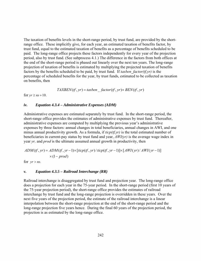
242

The taxation of benefits levels in the short-range period, by trust fund, are provided by the short-range office. These implicitly give, for each year, an estimated taxation of benefits factor, by trust fund, equal to the estimated taxation of benefits as a percentage of benefits scheduled to be paid. The long-range office projects these factors independently for every year of the projection period, also by trust fund. (See subprocess 4.1.) The difference in the factors from both offices at the end of the short-range period is phased out linearly over the next ten years. The long-range projection of taxation of benefits is estimated by multiplying the projected taxation of benefits factors by the benefits scheduled to be paid, by trust fund. If taxben_factor(tf,yr) is the percentage of scheduled benefits for the year, by trust funds, estimated to be collected as taxation on benefits, then

( , ) _ ( , ) ( , )TAXBEN tf yr taxben factor tf yr BEN tf yr= × for 10.yr ns≥ + iv. Equation 4.3.4 – Administrative Expenses (ADM) Administrative expenses are estimated separately by trust fund. In the short-range period, the short-range office provides the estimates of administrative expenses by trust fund. Thereafter, administrative expenses are computed by multiplying the previous year’s administrative expenses by three factors: annual changes in total beneficiaries, annual changes in AWI, and one minus annual productivity growth. As a formula, if ticp(tf,yr) is the total estimated number of beneficiaries in current-pay status by trust fund and year, AWI(yr) is the average wage index in year yr, and prod is the ultimate assumed annual growth in productivity, then

( , ) ( , 1) [ ( , ) / ( , 1)] [ ( ) / ( 1)](1 )

ADM tf yr ADM tf yr ticp tf yr ticp tf yr AWI yr AWI yrprod

= − × − × −× −

for .yr ns> v. Equation 4.3.5 – Railroad Interchange (RR) Railroad interchange is disaggregated by trust fund and projection year. The long-range office does a projection for each year in the 75-year period. In the short-range period (first 10 years of the 75-year projection period), the short-range office provides the estimates of railroad interchange by trust fund and the long-range projection is overridden in these years. Over the next five years of the projection period, the estimate of the railroad interchange is a linear interpolation between the short-range projection at the end of the short-range period and the long-range projection five years hence. During the final 60 years of the projection period, the projection is as estimated by the long-range office.

243

By trust fund, the total cost in calendar year yr, rr_cost(tf,yr) is the sum of railroad benefits and railroad administrative expenses, less the sum of railroad contributions and railroad taxation of benefits. By trust fund, the railroad interchange component of total cost is then equal to

( , ) [0.25 _ cost( , 2) 0.75 _ cost( , 1)] [1 1.25 ( )].RR tf yr rr tf yr rr tf yr yield yr= × − + × − × + Note that the railroad cost is increased by the yield rate on the combined OASDI trust funds for year yr. This formula takes into account the fact that that there is a delay from the end of the fiscal year to the time of valuation.

The total cost in year yr is broken down in to four components: railroad benefits in year yr, railroad administrative expenses in year yr, railroad contributions in year yr, and railroad taxation of benefits in year yr. The average railroad retired worker benefit is estimated to equal the average retired worker benefit, multiplied by the ratio of the railroad retirement benefit to the OASI retired worker benefit. The aggregate retired worker railroad benefits are estimated by multiplying the average railroad retired worker benefit by the number or railroad retirement beneficiaries. The number of railroad beneficiaries is estimated to be the previous year’s number of beneficiaries, decreased for survivorship plus the estimated number of new railroad employees for the year. The aggregate disabled worker railroad benefits (and beneficiaries) are estimated in the same way. It is assumed that the ratio of OASI taxation of benefits to OASI benefits and DI taxation of benefits to DI benefits are both the same for railroad taxation of benefits. The railroad taxation of benefits is estimated by multiplying the railroad benefits by these ratios. Administrative expenses are computed, by trust fund, to be the maximum of (a) and (b) where (a) is an estimated average cost per beneficiary times the number of beneficiaries and (b) is an estimated percentage of aggregate benefits times the aggregate railroad benefit levels. Railroad contributions are estimated, by trust fund, to be total railroad employment, multiplied by average railroad earnings, multiplied by the combined OASDI employer/employee tax rate. Railroad earnings are assumed to grow with the increase in the average wage index, and railroad employment is assumed to decrease over time. vi. Equation 4.3.6 – Interest Income (INT) In the short-range period, the projection of interest income by trust fund is provided by the short-range office. In each year of the short-range period, the annual yield rate is defined as the ratio of interest earned by a fund to the average level of assets held by the fund during the year.

244

The ultimate annual yield rate on each trust fund is equal to the nominal yield, which is the real interest rate increased for inflation. As a formula,

(1 ) (1 ) 1.ultimate yield rate real interest rate inflation rate= + × + − To get the yield rate for each year between the end of the short-range period and 5 years later when the ultimate yield rate is assumed to be reached, the program linearly interpolates between the values for these two years. The projection of interest income in a given year is the yield rate for that year multiplied by the average level of assets. As a formula,

( , ) ( , ) _ ( , ).INT tf yr yield tf yr avg assets tf yr= ×

The average level of assets in a trust fund, for a given year, is estimated to be the beginning of the year assets, increased by the tax contributions and taxation of benefits income (each exposed to the point in the year in which they are estimated to be received, on average), and decreased by scheduled benefits, railroad interchange, and administrative expenses (each exposed to the point in the year in which they are estimated to be disbursed, on average). For all years of the projection period, tax contributions are given an exposure of 0.525, taxation of benefits are given an exposure of 0.5, railroad interchange is given an exposure of 0.583, and administrative expenses are given an exposure of 0.5. For scheduled benefits, an exposure of 0.5 is ultimately given. The exposure, ben_exp(yr), is larger than 0.5 in the early years of the projection period and grades down smoothly to 0.5. The reason is that in the past, benefits were always paid at the beginning of each month. Now benefits are paid out throughout the month, based on the birth date of the beneficiary. The average assets held by the trust funds for a given year is estimated by the formula

_ ( , ) ( , ) 0.525 ( , )0.5 ( , ) ( ) ( , )

0.583 ( , ) 0.5 ( , ).

BOYavg assets tf yr ASSETS tf yr CONTRB tf yrTAXBEN tf yr ben_exp yr BEN tf yr

RR tf yr ADM tf yr

= + ×+ × − ×

− × − ×

vii. Equations 4.3.7, 4.3.8 and 4.3.9 – Annual Values The annual income rate for a trust fund is computed as the employer/employee tax rate for that fund, plus taxation of benefits as a percentage of taxable payroll.

( , )_ _ ( , ) ( , ) .( )

TAXBEN tf yrANN INC RT tf yr taxrate tf yrpayroll yr

= +

245

The annual cost rate for a trust fund is computed as the total cost of providing scheduled benefits from that fund as a percentage of taxable payroll. If

( , ) ( , ) ( , ) ( , ),COST tf yr BEN tf yr RR tf yr ADM tf yr= + + then

( , )_ _ ( , ) .( )

COST tf yrANN COST RT tf yrpayroll yr

=

The trust fund ratio measures the amount of beginning of year assets that can be used to pay scheduled benefits. It is expressed as a percentage.

( , )( , ) .( , )BOYASSETS tf yrTFR tf yr

BEN tf yr=

viii. Equations 4.3.10, 4.3.11, 4.3.12, and 4.3.13 – Summarized Values Present values of cash flows during the year are computed using the yield rate on the combined OASDI trust fund for that year. Each component of trust fund operations is exposed, with interest, to the point in the year in which, on average, it is received or disbursed. These exposure levels, ben_exp(yr), are the same as described above. These exposed levels are then discounted to January 1 of the year of the Trustees Report, ni. If yield(j) is the annual yield rate on the combined OASDI trust funds for year j and v(yr) is the discounting factor for the year, then

1( ) .[1 ( )]

yr

j ni

v yryield j=

=+∏

For a given year, and trust fund,

_ ( , ) (1 0.525 ( )) ( , ) ( ),_ ( , ) (1 0.5 ( )) ( , ) ( ),

_ ( , ) (1 _ ( ) ( )) ( , ) ( ),_ ( , ) (1 0.583 ( )) (

PV TAX tf yr yield yr TAX tf yr v yrPV TAXBEN tf yr yield yr TAXBEN tf yr v yr

PV BEN tf yr ben exp yr yield yr BEN tf yr v yrPV RR tf yr yield yr RR t

= + × × ×= + × × ×= + × × ×

= + × × , ) ( ),and _ ( , ) (1 0.5 ( )) ( , ) ( ).

f yr v yrPV ADM tf yr yield yr ADM tf yr v yr

×= + × × ×

The target fund for a year is next year’s cost. Its present value is computed as

_ ( , ) [ ( , 1) ( , 1) ( , 1)] ( ),PV TARG tf yr BEN tf yr RR tf yr ADM tf yr v yr= + + + + + × Taxable payroll is exposed to the middle of the year when computing present values:

_ ( ) (1 0.5 ( )) ( ) ( ).PV PAYROLL yr yield yr payroll yr v yr= + × × ×

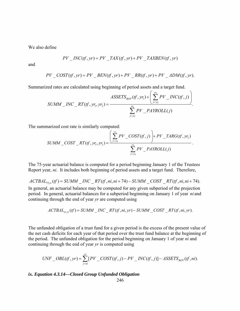
246

We also define

_ ( , ) _ ( , ) _ ( , )PV INC tf yr PV TAX tf yr PV TAXBEN tf yr= +

and

_ ( , ) _ ( , ) _ ( , ) _ ( , ).PV COST tf yr PV BEN tf yr PV RR tf yr PV ADM tf yr= + + Summarized rates are calculated using beginning of period assets and a target fund.

2

1

2

1

1

1 2

( , ) _ ( , )_ _ ( , , ) .

_ ( )

yr

BOYj yr

yr

j yr

ASSETS tf yr PV INC tf jSUMM INC RT tf yr yr

PV PAYROLL j

=

=

⎛ ⎞+ ⎜ ⎟⎝ ⎠=∑

∑

The summarized cost rate is similarly computed:

2

1

2

1

2

1 2

_ ( , ) _ ( , )_ _ ( , , ) .

_ ( )

yr

j yryr

j yr

PV COST tf j PV TARG tf yrSUMM COST RT tf yr yr

PV PAYROLL j

=

=

⎛ ⎞+⎜ ⎟

⎝ ⎠=∑

∑

The 75-year actuarial balance is computed for a period beginning January 1 of the Trustees Report year, ni. It includes both beginning of period assets and a target fund. Therefore,

75 ( ) _ _ ( , , 74) _ _ ( , , 74).yrACTBAL tf SUMM INC RT tf ni ni SUMM COST RT tf ni ni= + − + In general, an actuarial balance may be computed for any given subperiod of the projection period. In general, actuarial balances for a subperiod beginning on January 1 of year ni and continuing through the end of year yr are computed using

, ( ) _ _ ( , , ) _ _ ( , , ).ni yrACTBAL tf SUMM INC RT tf ni yr SUMM COST RT tf ni yr= −

The unfunded obligation of a trust fund for a given period is the excess of the present value of the net cash deficits for each year of that period over the trust fund balance at the beginning of the period. The unfunded obligation for the period beginning on January 1 of year ni and continuing through the end of year yr is computed using

_ ( , ) [ _ ( , ) _ ( , )] ( , ).yr

BOYj ni

UNF OBL tf yr PV COST tf j PV INC tf j ASSETS tf ni=

= − −∑

ix. Equation 4.3.14—Closed Group Unfunded Obligation

247

The closed group is defined as individuals who attain specified ages in the first year of the projection period (ni). The Statement of Social Insurance displays unfunded obligations for closed groups (1) attaining 15 or later in 2008, (2) attaining 62 or older in 2008, and (3) attaining 15 to 61 in 2008. For each year of the projection period, closed group calculations attribute a portion of the items in equations 4.3.1 through 4.3.6 to individuals falling in the defined closed group. The calculation of the closed-group unfunded obligation, then, uses the equation above but only considering the present values of cost and income attributable to the closed group. The following information, developed elsewhere in the “Cost” process, is used for developing closed group unfunded obligation amounts:

• Total number of workers and total taxable earnings by single year of age 15-74 and sex, years 1951 through nf, updated yearly

• Taxable payroll, years ni through nf, updated yearly • Payroll tax income, years ni through nf, updated yearly • Income from taxation of benefits, years ni through nf, updated yearly • Scheduled benefits by beneficiary category, years ni through nf, updated yearly • Railroad interchange, years ni through nf, updated yearly • Administrative expenses, years ni through nf, updated yearly • Yield rate on the combined OASDI trust funds, years ni through nf, updated yearly

It is important to note that, for dependent beneficiaries, the age of the worker, on whose account the benefits are based, determines whether that beneficiary would fall in the closed group. For instance, if the closed group were defined as individuals attaining age 15 or later in 2008 and in 2008 a 3-year-old minor child was receiving benefits on the account of a retired worker aged 63, the minor child beneficiary would be considered as part of this closed group because the account holder was at least age 15 in 2008. The following describes how the various components of income and cost are allocated to the defined closed group in question:

Payroll Tax Contributions Closed group taxable payroll is defined as the percentage of OASDI taxable payroll attributable to the closed group in question. An input file of closed group payroll factors, containing these percentages by year from 2008 through 2107, is used by the cost program to compute payroll tax contributions attributable to the closed group. For each year, the closed group payroll factors are determined as follows:

• The number of projected workers by single year of age (ages 1-99) and sex are multiplied by the associated average earnings by age/sex.

• Then, the portion of total taxable earnings attributable to the closed group is calculated.

248

For each year of the projection period, the number of workers and average taxable earnings by single year of age and sex are determined as follows:

• For ages 15-74, the number of projected workers comes directly from Economics group projections, and the average earnings by age and sex comes directly from the AWARDS subprocess.

• For ages 1-14, the number of projected workers is obtained by averaging the percentage of workers at each age relative to the total 1-14 age group, using 14 years of earnings data (1991-2004) in the averaging calculations. Average taxable earnings for ages 1-14 are obtained by analyzing historical 1991-2004 data of the average earnings at each age relative to the age 15 average earnings, and judgmentally assigning a ratio (to age 15 average earnings) for each age.

• For ages 75-99, the number of projected workers by age and sex is obtained through first developing the ratio of workers in 2004 at each age to the projected population in 2004 at that age and then applying that ratio to projected population by age in years 2007 and later. Then, the resulting estimated workers are adjusted by an equivalent percentage to match the total number of projected workers aged 75 and later, as provided by the Economics group. This process is done separately by sex. To obtain the average taxable earnings for single years of age 75-99, ratios of average earnings by age 75-99 to overall average earnings for all ages is computed for each age 75-99, for earnings years 1991 through 2004. These ratios by age are then averaged for all 14 years, from which earnings ratios to overall average earnings are developed judgmentally. This process is done separately by sex.

Benefits Methodologies for computing benefits attributable to the closed groups differs among benefit categories, as described below:

Retired Workers For each age in current pay, the number of beneficiaries is multiplied by the corresponding average benefit amount across all ages of entitlement. The same applies for DI conversion cases. Retroactive benefits for the current year, by age, are then calculated. The closed-group factors for old-age benefits for each year are found by summing the benefit amounts attributable to the specified closed group, as a proportion of total retired worker benefits for all ages. This process is done separately by sex.

Disabled Workers For each age from 20 to the year before normal retirement age, the program adds the products of the number of beneficiaries for each duration and the PIA for that duration. Retroactive benefits for the current year, by age, are then calculated. The closed-group

249

factors for disability benefits are found by summing the total benefit amounts attributable to the closed group, as a proportion of total disabled worker benefits for all ages. This process is done separately by sex. Aged Spouses The number of aged wife beneficiaries in current pay status (no dual entitlement) is provided by single year of age. Then, for each single year of age, the program allocates total numbers of husbands by age, from 5 years younger to 12 years older than the aged wife using an assumed distribution. Next, for each age of husband in current pay, the number of husbands is multiplied by the weighted average retired worker benefit across all ages of entitlement. The closed group factors, then, are obtained by determining the proportion of total benefit amounts attributable to the given closed group (based on the husband’s age). The same closed group factors are applied to the excess benefit amount for aged wives in dual entitlement status (i.e. aged wives with a smaller worker benefit). Aged husbands, a very small beneficiary group, get the same closed group benefit factors as do the aged wives, described above. Aged Widows The number of aged widow beneficiaries in current pay status (no dual entitlement) is provided by age from 60 to 95. For each single year of age, the program allocates total number of aged widows by age of the deceased husband (age the husband would have been if he had not died), from 10 years younger to 15 years older than the aged widow using an assumed distribution. For each age of deceased husband aged 95 or younger, a real wage growth factor is applied to reflect ultimate real wage growth taken to the power to the number of years younger than age 96.

)ker96()028.1/039.1( agewordeceasedBenefitadj −= This exponent is intended to reflect differences in average levels of benefits, with younger deceased husbands having higher benefits based on real wage growth. The closed group factors, then, are obtained by determining the proportion of total benefit amounts attributable to the closed group The same closed group factors are applied to excess benefit amounts for aged widows in dual entitlement status (i.e. aged widows with a smaller worker benefit). Aged widowers receive the same closed group benefit factors as do aged widows (based on the deceased husband’s age). Other Beneficiary Categories

250

For the 20 other dependent beneficiaries of retired workers, disabled workers, and deceased workers, an input file of closed group benefit factors is created, which represents the proportion of total (open-group) projected benefits in that category attributable to the given closed group age and year. This file is used by the cost program to compute amounts from each beneficiary category attributable to the closed group. The file, separately created for each closed group run, contains closed group benefit factors for ages 0 through 150 for each of the 20 beneficiary categories by sex of the account holder (worker). These input files are created by examining a recent sample of Master Beneficiary Record (MBR) data1 for each of the beneficiary categories by age of the worker, and projecting future distributions by age of the worker based on population and, for survivor benefits, projected deaths by age. Then, adjustments are made for real wage growth to reflect different benefit levels by birth cohort.

Taxation of Benefits

Since taxation of benefits is related to benefits, the closed-group taxation of benefit amounts are computed by multiplying the total (open-group) taxation of benefit amounts by Trust Fund, by the corresponding total closed-group benefit factors by Trust Fund.

Administrative Expenses Since administrative expenses are also assumed to be related to benefits, the closed-group administrative expense amounts are computed by multiplying the total (open-group) administrative expenses by Trust Fund), by the corresponding total closed-group benefit factors by Trust Fund.

Railroad Interchange Since the railroad interchange has both a payroll tax and benefit component, each component is multiplied by its corresponding closed-group factor. That is, total payroll tax contributions arising from railroad interchange are multiplied by the closed group payroll factor discussed above in the “Tax on Contributions” section. Total railroad benefits, by Trust Fund, are multiplied by the aggregate closed-group benefit factors by Trust Fund. Closed-group railroad administrative expenses and closed-group railroad taxation of benefits are also estimated by applying aggregate closed group benefit factors by Trust Fund. The final amount is then the difference in the components (closed group railroad income less closed group railroad cost).

251

Appendix 4.3-1 Shuttling Method

In this appendix we discuss the “shuttling method”. The shuttling method as presented in the COST model attempts to reorganize the PAPs obtained from subprocess 4.2, which maintains a static age-sex distribution of newly entitled beneficiaries, in such a way that captures the changing age-sex distribution of newly entitled beneficiaries provided by subprocess 3.3. The age-sex distribution of the sample (subprocess 4.2) and those newly entitled from subprocess 3.3 are aligned in the sample year. This alignment persists throughout all years in the long-range period. When we refer to the age-sex distribution fom subprocess 3.3 in what follows below, we refer to the aligned age-sex distribution. Let oadsrs be the age/sex distribution of the sample from subprocess 4.2. Let oabicp be the number of newly entitled beneficiaries by age and sex from subprocess 3.3. Let total be the total number of newly entitled beneficiaries by sex. The ratio

( , ) ,( )

oabicp sex agetotal sex

for age = 62, … , 70 gives the age-sex distribution from subprocess 3.3.

The array rsb_oadscp_sampleyr is the age-sex distribution from subprocess 3.3 from the sample year (2004 for the 2008 Trustees Report).

The value of oadscp is defined, by age and sex, to be:

( , )( , ) ( , ) _ _ ( , ).( )

oabicp sex ageoadscp sex age oadsrs sex age rsb oadscp sampleyr sex agetotal sex

= + −

We will call this the aligned age-sex distribution as obtained from subprocess 3.3. For each sex, we construct a matrix oads. Construction of this matrix uses two different age-sex distributions: the age-sex distribution of the awards sample and the aligned age-sex distribution of newly entitled beneficiaries from subprocess 3.3. The matrix oads is a 9 9× matrix whose rows and columns are indexed consecutively by the ages 62,…, 70. We index the rows of this matrix by the age of entitlement of a worker in the projection (ageentRSB) and the columns of this matrix by the age of entitlement of a worker in the Awards sample (ageentAWD). More precisely, for a given sex, let oadsrs be the age distribution of the sample; oadscp be the aligned age distribution of newly entitleds from subprocess 3.3. Both arrays oadsrs and oadscp are indexed by age, ages = 62, …, 70. For a given sex, the matrix oads is constructed with the following properties:

70

62( ) ( , )

ageentAWDoadscp ageentRSB oads ageentRSB ageentAWD

=

= ∑

and

252

70

62( ) ( , ).

ageentRSBoadsrs ageentAWD oads ageentRSB ageentAWD

=

= ∑

In other words, the matrix oads has the following properties:

• The sum of the entries in any row of the matrix is the value of the distribution of the projection for the age corresponding to the row.

• The sum of the entries in any column of the matrix is the value of the distribution of the Awards sample for the age corresponding to the column.

Let opap be the original potential AIME percentages (PAPs) passed to subprocess 4.3 from subprocess 4.2. This is a 9 10× matrix whose rows are indexed by ages at entitlement 62, …, 70 and whose columns are indexed by benefit interval 1, …, 10 (represented by the variable i in the formulas below). The values of opap are modified and the results are the PAPs used by process 4.3, called opap1. As a formula,

70

6270

62

1( , )

( , ) ( , ).

( , )

ageentAWD

ageentAWD

opap ageentRSB i

opap ageentAWD i oads ageentRSB ageentAWD

oads ageentRSB ageentAWD

=

=

×=

∑

∑

This formula may be rewritten as follows.

70

7062

62

1( , )( , )( , ) .

( , )=

=

= ×∑∑ageentAWD

ageentAWD

opap ageentRSB ioads ageentRSB ageentAWDopap ageentAWD i

oads ageentRSB ageentAWD

It follows that opap1 may be interpreted as a reweighting of opap. We have 70

,62

1( , ) ( , )ageentRSB ageentAWDageentAWD

opap ageentRSB i w opap ageentAWD i=

= ×∑

with weights ,( , ) .

( )ageentRSB ageentAWDoads ageentRSB ageentAWDw

oadscp ageentRSB=

As matrices, 1opap w opap= × (and is another 9 10× matrix). Consider the following example. In this example, the projection year is 2040, and the sex is males. The oadsrs vector (from subprocess 4.2) is as follows.

62 63 64 65 66 67 68 69 70Male 0.4615 0.1466 0.0676 0.2533 0.0555 0.0058 0.0036 0.0030 0.0030

The unaligned age-sex distribution (from subprocess 3.3) is as follows.

253

62 63 64 65 66 67 68 69 70Male 0.3501 0.1383 0.0514 0.1303 0.1196 0.2206 0.0096 0.0136 0.0117

The age-sex distribution (from subprocess 3.3) in 2004, the year of the sample is as follows.

62 63 64 65 66 67 68 69 70Male 0.4362 0.1521 0.0694 0.2460 0.0800 0.0059 0.0017 0.0024 0.0062

Hence the aligned age-sex distribution (from subprocess 3.3), that is, the oadscp vector, is as follows.

62 63 64 65 66 67 68 69 70Male 0.3304 0.1328 0.0496 0.1376 0.0951 0.2205 0.0115 0.0142 0.0085

The matrix oads, computed in this subprocess (4.3) is as follows. An explanation of how this matrix is generated appears below.

\ 62 63 64 65 66 67 68 69 70 Total62 0.3304 0.0000 0.0000 0.0000 0.0000 0.0000 0.0000 0.0000 0.0000 0.330463 0.1311 0.0016 0.0000 0.0000 0.0000 0.0000 0.0000 0.0000 0.0000 0.132864 0.0000 0.0496 0.0000 0.0000 0.0000 0.

ageentRSB ageentAWD

0000 0.0000 0.0000 0.0000 0.049665 0.0000 0.0954 0.0422 0.0000 0.0000 0.0000 0.0000 0.0000 0.0000 0.137666 0.0000 0.0000 0.0254 0.0696 0.0000 0.0000 0.0000 0.0000 0.0000 0.095167 0.0000 0.0000 0.0000 0.1837 0.0368 0.0000 0.0000 0.0000 0.0000 0.220568 0.0000 0.0000 0.0000 0.0000 0.0115 0.0000 0.0000 0.0000 0.0000 0.011569 0.0000 0.0000 0.0000 0.0000 0.0072 0.0058 0.0012 0.0000 0.0000 0.014270 0.0000 0.0000 0.0000 0.0000 0.0000 0.0000 0.0024 0.0030 0.0030 0.0085

Total 0.4615 0.1466 0.0676 0.2533 0.0555 0.0058 0.0036 0.0030 0.0030 1.0000

Note that the column total is oadsrs and the row total is oadscp. The oads matrix is determined using these row and column sum constraints. The nonzero entries of the oads matrix zig-zag down and to the right. Starting at the upper left hand corner, the lesser of oadsrs and oadscp is put there. So (62,62) 0.3304.oads = In this case (as is usually the case) oadscp is less. The difference (62) (62) 0.4615 0.3304 0.1311oadsrs oadscp− = − = is placed one lower, in (63,62).oads Since the sum of the first column is (62)oadsrs and the sum of the first row is (62),oadscp we move to the next entry on the right. The difference

(63) (63,62) 0.1328 0.1311 0.0016,oadscp oads− = − = is (63,63).oads Now we have that the row sum is (63).oadscp We want the column sum to be (63).oadsrs We move down to

(64,63).oads Since (63) (63,63) 0.1466 0.0016 0.1450 0.1328 (63),oadsrs oads oadscp− = − = > = by the row sum

constraint we are forced to have (64,63) 0.0496.oads = Now move one lower. Since 0.1466 0.0496 0.0016 0.0954 (65) 0.1376,oadscp− − = < = the entry (65,63) 0.0954.oads = The column sum is now (63),oadsrs and we move one over to the right. We want to fill in this entry. We compute (65) (65,62) 0.1376 0.0954 0.0422 0.0676,oadscp oads− = − = < by the column sum constraint we have (65,64) 0.0422.oads = The row constraint is now met, and we

254

move down to (66,64).oads We look at (66) 0.0951.oadscp = By the column constraint, we cannot place this value in (66,64).oads So to meet the column constraint, we set

(66,64)oads equal to the difference (64) (65,64) 0.0676 0.0422 0.0254.oadsrs oads− = − = Now that this column constraint is met, we move one column over to (66,65).oads Note that we cannot put (65) 0.2533oadsrs = there since then the row constraint would be violated. In order to meet the row constraint,

(66,65) (66) (66,64) 0.0951 0.0254 0.0696.oads oadscp oads= − = − = Since the row constraint is met, we move one row down to (67,65).oads We cannot put (67)oadscp there since then the column constraint would be violated. Hence

(67,65) (65) (66,65) 0.2533 0.0696 0.1837.oads oadsrs oads= − = − = Now that the column constraint is met, we move one column over to (67,66).oads We cannot put

(66) 0.0555oadsrs = there or else the row constraint would be violated. So we put (67,66) (67) (67,65) 0.2205 0.1837 0.0368oads oadscp oads= − = − = there. Now the row

constraint is met and we move one row down to (68,66).oads Since (67,66) (68) (66),oads oadscp oadsrs+ < we have (68,66) (66) 0.0115.oads oadscp= = Now

move one row down to (69,66).oads We cannot put (69) 0.0142oadscp = there or else the column constraint would be violated. Hence

(69,66) (66) (67,66) (68,66) 0.0555 0.0368 0.0115 0.0072oads oadsrs oads oads= − − = − − = and the column constraint is met. Now move one column over to (69,67).oads We put

(69,67) (67) 0.0058oads oadsrs= = there since that meets the column constraint and the row constraint remains unsatisfied. So move over to the next column, (69,68).oads We cannot put (68)oadsrs there since that would violate the row constraint. It follows that

(69,68) (69) (69,66) (69,67) 0.0142 0.0072 0.0058 0.0012.oads oadscp oads oads= − − = − − = Now the row constraint is satisfied and we move down to the last row and (70,68).oads By the column constraint, this entry is forced to be 0.0024. Moving to column 69, again, by the column constraint, the entry (70,69)oads is forced to be 0.0030. Finally, by the row and column constraints, the last entry, (70,70),oads is 0.0030. To obtain the w matrix, normalize the rows by dividing by the row sum.

\ 62 63 64 65 66 67 68 69 7062 1.0000 0.0000 0.0000 0.0000 0.0000 0.0000 0.0000 0.0000 0.000063 0.9877 0.0123 0.0000 0.0000 0.0000 0.0000 0.0000 0.0000 0.000064 0.0000 1.0000 0.0000 0.0000 0.0000 0.0000 0.0000 0.0000 0

ageentRSB ageentAWD

.000065 0.0000 0.6935 0.3065 0.0089 0.0000 0.0000 0.0000 0.0000 0.000066 0.0000 0.0000 0.2676 0.7324 0.0000 0.0000 0.0000 0.0000 0.000067 0.0000 0.0000 0.0000 0.8331 0.1669 0.0000 0.0000 0.0000 0.000068 0.0000 0.0000 0.0000 0.0000 1.0000 0.0000 0.0000 0.0000 0.000069 0.0000 0.0000 0.0000 0.0000 0.5094 0.4085 0.0822 0.0000 0.000070 0.0000 0.0000 0.0000 0.0000 0.0000 0.0000 0.2852 0.3516 0.3516

255

Then, as matrices, 1 ,opap w opap= × as one may verify. For display purposes the transposes of opap and opap1 are shown.

opap 62 63 64 65 66 67 68 69 70

1 0.9993 0.9992 0.999 0.9985 0.9985 0.9964 0.9929 0.99 0.9893 2 0.989 0.9895 0.986 0.9867 0.9828 0.9245 0.9302 0.9004 0.9163 3 0.9635 0.9676 0.9627 0.9665 0.9551 0.8182 0.7771 0.7245 0.8272 4 0.9336 0.9431 0.9318 0.9462 0.9318 0.7063 0.6486 0.5597 0.7364 5 0.9037 0.9163 0.9068 0.9264 0.9131 0.6373 0.563 0.4703 0.6687 6 0.8768 0.8913 0.8831 0.9073 0.8909 0.5994 0.5017 0.4193 0.6242 7 0.8499 0.8671 0.8588 0.888 0.8697 0.5663 0.4846 0.3943 0.5957 8 0.8235 0.843 0.8362 0.869 0.8525 0.5333 0.4495 0.3733 0.5577 9 0.7953 0.8178 0.8148 0.8501 0.8363 0.5065 0.4162 0.3587 0.5398

10 0.7692 0.789 0.7913 0.8308 0.8191 0.4839 0.386 0.3395 0.5064 11 0.7432 0.7613 0.7674 0.8098 0.8009 0.4617 0.3621 0.325 0.4707 12 0.7157 0.7324 0.7419 0.7884 0.7849 0.4435 0.3485 0.3071 0.4401 13 0.688 0.7015 0.7139 0.7649 0.762 0.4328 0.3264 0.2848 0.4118 14 0.6386 0.6465 0.6671 0.7213 0.7238 0.3989 0.297 0.2557 0.3861 15 0.5689 0.5702 0.5968 0.6564 0.6685 0.3558 0.2653 0.228 0.3386 16 0.495 0.4916 0.52 0.5887 0.6098 0.3277 0.2338 0.2053 0.302 17 0.4218 0.4139 0.4441 0.5201 0.5432 0.3014 0.2124 0.1901 0.2823 18 0.3502 0.3422 0.3773 0.4561 0.4796 0.2719 0.1857 0.182 0.259 19 0.2534 0.2513 0.2875 0.366 0.3974 0.2413 0.1608 0.1624 0.2315 20 0.1481 0.1571 0.1882 0.263 0.293 0.1944 0.1349 0.1294 0.1887 21 0.0731 0.0816 0.1056 0.1676 0.1979 0.1457 0.0998 0.1025 0.1405 22 0.0232 0.0282 0.0421 0.0709 0.094 0.0841 0.0631 0.0641 0.0824 23 0.0036 0.0051 0.0102 0.017 0.0231 0.0248 0.0268 0.023 0.0281 24 0 0 0 0 0.0004 0.0007 0.0024 0.0018 0.0038 25 0 0 0 0 0 0 0 0 0 26 0 0 0 0 0 0 0 0 0 27 0 0 0 0 0 0 0 0 0 28 0 0 0 0 0 0 0 0 0 29 0 0 0 0 0 0 0 0 0 30 0 0 0 0 0 0 0 0 0

256

opap1 62 63 64 65 66 67 68 69 70

1 0.9993 0.9993 0.9992 0.9991 0.9986 0.9985 0.9985 0.9972 0.979 2 0.989 0.989 0.9895 0.9884 0.9865 0.986 0.9828 0.9547 0.9039 3 0.9635 0.9636 0.9676 0.9661 0.9655 0.9646 0.9551 0.8846 0.7671 4 0.9336 0.9337 0.9431 0.9396 0.9423 0.9438 0.9318 0.8164 0.6406 5 0.9037 0.9039 0.9163 0.9134 0.9212 0.9242 0.9131 0.7717 0.561 6 0.8768 0.877 0.8913 0.8888 0.9008 0.9046 0.8909 0.7398 0.5099 7 0.8499 0.8501 0.8671 0.8646 0.8802 0.8849 0.8697 0.7141 0.4862 8 0.8235 0.8237 0.843 0.8409 0.8602 0.8662 0.8525 0.689 0.4555 9 0.7953 0.7956 0.8178 0.8169 0.8407 0.8478 0.8363 0.6671 0.4346

10 0.7692 0.7694 0.789 0.7897 0.8202 0.8288 0.8191 0.6466 0.4075 11 0.7432 0.7434 0.7613 0.7632 0.7985 0.8083 0.8009 0.6263 0.383 12 0.7157 0.7159 0.7324 0.7353 0.776 0.7878 0.7849 0.6096 0.3621 13 0.688 0.6882 0.7015 0.7053 0.7513 0.7644 0.762 0.5917 0.338 14 0.6386 0.6387 0.6465 0.6528 0.7068 0.7217 0.7238 0.556 0.3103 15 0.5689 0.5689 0.5702 0.5784 0.6404 0.6584 0.6685 0.5076 0.2748 16 0.495 0.495 0.4916 0.5003 0.5703 0.5922 0.6098 0.4637 0.245 17 0.4218 0.4217 0.4139 0.4232 0.4998 0.524 0.5432 0.4172 0.2266 18 0.3502 0.3501 0.3422 0.353 0.435 0.46 0.4796 0.3706 0.208 19 0.2534 0.2534 0.2513 0.2624 0.345 0.3712 0.3974 0.3142 0.1843 20 0.1481 0.1482 0.1571 0.1666 0.243 0.268 0.293 0.2397 0.1503 21 0.0731 0.0732 0.0816 0.089 0.151 0.1727 0.1979 0.1685 0.1139 22 0.0232 0.0233 0.0282 0.0325 0.0632 0.0748 0.094 0.0874 0.0695 23 0.0036 0.0036 0.0051 0.0067 0.0152 0.018 0.0231 0.0241 0.0256 24 0 0 0 0 0 0.0001 0.0004 0.0007 0.0027 25 0 0 0 0 0 0 0 0 0 26 0 0 0 0 0 0 0 0 0 27 0 0 0 0 0 0 0 0 0 28 0 0 0 0 0 0 0 0 0 29 0 0 0 0 0 0 0 0 0 30 0 0 0 0 0 0 0 0 0

long-range oasdi projection methodology · long-range oasdi projection methodology intermediate...

Documents