i

Loss and Ambiguity Aversion and the Willingness

to Pay for Index Insurance:

Experimental Evidence from Rural Kenya

Edwin Slingerland

Abstract

This study looks at the impact ambiguity attitudes and loss aversion might have on willingness-to-pay

for index insurance among 13 farmer groups in rural Kenyan farmers. Basis risk is a source of

ambiguity which is considered a barrier for index insurance uptake. In a framed field experiment, we

test whether a rebate insurance, where the premium payment is no longer certain but probable,

increases WTP. We find no significant difference in WTP for the two designs. We do find widespread

insensitivity to ambiguity generated likelihoods which significantly reduces WTP for index insurance

due to overweighting the probability of basis risk. Surprisingly we find that the negative effect on

WTP of pessimistic people is significantly larger for the rebate insurance than for the traditional

insurance. Our findings are in line with Prospect Theory and contribute to understanding how

farmers’ perceive index insurance designs, underlining the need to experiment with alternative

insurance designs taking into account ambiguity attitudes and with less basis risk.

Supervisors: Prof. Robert Lensink, Francesco Cecchi

Date: 28/09/2017

Chair group: Development Economics (DEC)

Thesis code: DEC-80433

ii

Acknowledgement Hakuna Matata is not the most appropriate term I would use to describe the process of writing this

thesis. It was definitely not always easy and I would like to thank my supervisors Robert Lensink and

Francesco Cecchi for taking away any worries I might have had. I appreciate all the support and

stimulating feedback and the opportunity to conduct my master thesis in Kenya. It has been a great

experience to conduct my own research and collect my own data, from which I learned a lot. I would

like to mention Francesco Cecchi especially for all the guidance throughout the whole process, for

keeping on challenging me and for tirelessly helping me devise new creative ways to measure

ambiguity attitudes. I also could not have done it without the help of Sister Sara, Sister Ruth and

Sister Jenerusa. It was a pleasure to stay at the convent in Meru, where you took great care of me

and kept reminding me to eat when I was stressed out. I would also like to thank Lawi for helping me

in organising the logistics of my research and any other things that needed to be arranged. Collecting

the data would not have been possible without the help of all of the enumerators. You guys did such

an amazing job and never complained, even if we had to walk for half an hour due to muddy roads

with all the materials and chairs. We had such good times together, whether it was in the field or in

The Underground in the weekend. I’m glad I was able to develop friendships with some of you and

got to experience more of Kenyan culture. Finally, I would like to thank my partner in crime

Annemarie Ionescu, with whom I was blessed to spend my time in Kenya with. I believe we work

great as a team and I thoroughly enjoyed all those special moments: going crazy from sleep

deprivation and sorting a bazillion beads, being stuck in the chapel at midnight surrounded by the

convent’s guard dogs or spotting the Big 5 on Safari.

iii

Contents 1. Introduction ....................................................................................................................... 1

2. Literature Review and Theoretical Framework ......................................................................... 3

2.1: A history of uncertainty and ambiguity in decision science ......................................................... 3

2.2: Ambiguity Attitudes: ambiguity aversion and a-insensitivity ....................................................... 5

2.3 Prospect Theory ................................................................................................................... 6

2.4: Insurance contract design ..................................................................................................... 8

2.5 Synthesis and Hypotheses ..................................................................................................... 9

3. Experimental Design and Methodology ................................................................................. 12

3.1: Sample ............................................................................................................................ 12

3.2: Incentives ........................................................................................................................ 13

3.3: Game 1: Measuring Ambiguity Attitudes ............................................................................... 14

Elicitation Procedure .............................................................................................................. 14

Estimating Ambiguity Aversion ................................................................................................ 15

Check questions and Pay-Out .................................................................................................. 16

Estimating A-insensitivity ....................................................................................................... 17

Ambiguity attitudes for Losses................................................................................................. 17

Practicalities ......................................................................................................................... 17

3.4: Game 2: Measuring Loss Aversion ....................................................................................... 18

Procedural details .................................................................................................................. 18

Estimating Loss Aversion ........................................................................................................ 19

3.5: Game 3: eliciting WTP for Insurance designs ......................................................................... 21

Experimental set-up .............................................................................................................. 22

Procedural details .................................................................................................................. 23

3.6: Methodology ..................................................................................................................... 24

4. Results and Analysis .......................................................................................................... 27

4.1: Ambiguity Game .............................................................................................................. 27

4.2: Loss aversion .................................................................................................................... 29

4.3: Willingness-to-Pay and Analysis ........................................................................................... 31

5. Discussion ........................................................................................................................... 34

6. Conclusion ....................................................................................................................... 36

7. References ....................................................................................................................... 37

Appendix A: Overview of definitions ............................................................................................ 41

Appendix B ............................................................................................................................. 42

1

1. Introduction Index insurance is considered a promising risk-coping strategy for households in developing

countries. Recent studies find a positive effect of insurance on technology adoption (Hill & Viceisza,

2012), employment of riskier and higher yielding inputs (de Nicola & Hill, 2013) such as fertilizer,

seeds and land. Cai (2016) finds higher investments among insured farmers as well as higher

consumptions. Janzen and Carter (2013) find a negative correlation between index insurance and

distress livestock sales in Kenya. Index insurance’s pay-out is based on indices such as satellite images

or weather stations measuring rainfall. This overcomes the high transaction costs and information

asymmetry problems that constitute barriers for the market of traditional insurance in developing

countries. In theory, this could greatly improve access to insurance for the poor and enable them to

smoothen income, stimulate investments, increase their revenues and escape potential poverty

traps. Unfortunately, uptake of index-insurance, has been rather low (Cole et al., 2013).

Paradoxically, index insurance is particularly undemanded by the risk averse (Falco et al., 2016). The

literature on microinsurance attributes the low uptake to financial illiteracy, trust, poor marketing,

credit/liquidity constraints and price. Another reason is basis risk, which can be defined as the

imperfect correlation between the indemnity payments and the actual losses of the farmer. Indices

that measure rainfall for example, are not always accurate for every farmer. Therefore, an insured

farmer that experiences a drought, is not paid out if the index measured enough rain in his region.

The probability of this happening is unknown to the farmer which constitutes a situation of

ambiguity. Ambiguity is different from risk, for which the probability is objective. Both are considered

sources of uncertainty. In general economic agents are ambiguity averse, meaning that people prefer

to bet on an option with known probabilities than on an option with unknown probabilities (Attanasi

et al., 2014). It is seen as a fixed trait of character and can also be interpreted as pessimism (Wakker,

2010). Falco et al. (2016) find that in ambiguous situations people rely on heuristic tools to make

investment decisions, such as past experiences or experiences of friends and family. Moreover,

index-insurance constitutes a double or compound lottery of either a good or bad harvest and of the

index being valid or invalid. Elabed and Carter (2015) show that 66% of cotton farmers in Mali are

compound-risk averse, which is strongly correlated to ambiguity aversion (Halevy, 2007), cutting

down demand for index insurance in half relative to expected utility theory.

In studies on index-insurance and ambiguity, the focus has been solely on ambiguity aversion. The

literature on decision making and ambiguity, however, shows a more diverse pattern of responses to

ambiguous situations. Some people tend to be more pessimistic, others are more optimistic. Various

studies have found that this response to ambiguity is dependent on whether it is gain or a loss and

on the degree of likelihood of the ambiguous event (Baillon & Bleichrodt, 2015; Abdellaoui, 2011;

Dimmock et al., 2015). They also observe a second important part of ambiguity, called ambiguity

generated insensitivity or a-insensitivity, which is defined as the inability to sufficiently discriminate

between different levels of ambiguity, transforming likelihoods towards fifty-fifty (Wakker, 2010).

This is the first study that analyses the full variety of ambiguity attitudes in relation to index

insurance. Moreover, to our knowledge this study is the first of its kind that measures ambiguity

attitudes of a sample of subsistence farmers in Africa. To this end, we adapted and simplified the

methodology of Dimmock et al. (2015) and investigated whether the same results are obtained as

found on a Western population. Finally, This study explores which type of ambiguity attitudes have

an impact on willingness-to-pay (hereafter WTP) for index insurance with basis risk and whether a

different frame of insurance could lead to higher WTP. We tested this by offering half the sample a

traditional index insurance and the other half a rebate type insurance, where the payment of the

premium only occurs in good years. In bad years the premium is deducted from the pay-out for the

2

rebate type. They are actuarially equivalent, but differ in framing of the insurance. Serfilippi et al.

(2016) do a similar WTP-experiment and find that subjects who overvalue certainty, have a

significantly higher WTP for the rebate type of insurance, as the certain loss of paying the premium

has changed from being a certain loss, to a probable loss. A shortcoming of this research is that they

did not include basis risk, which seems to be an important barrier for insurance uptake.

Ambiguity aversion was first discovered by Ellsberg in 1964, challenging Expected Utility theory (EU).

EU is good in predicting how people should behave, but fails in practice when trying to explain an

individual’s decision making (al-Nowaihi and Dhami, 2010). The human mind is limited when making

decisions that require complex decision making. Uncertain situations – with or without known

probabilities – can be very complex leading to suboptimal decision making. Kahneman and Tversky’s

(1992) Prospect Theory does provide tools to allow for such limitations. Wakker (2010), Baillon and

Bleichrodt (2015) and Abdellaoui (2011) claim that Prospect Theory is the best model to explain the

variety of behaviour found in individual decision making in ambiguous situations.

This research took place in Meru County, Kenya in May 2017. In total 276 female subsistence

farmers, from 13 different farmer groups, took part in our study. They participated in three separate

games eliciting their ambiguity attitudes for gains and losses, loss aversion and WTP for two types of

index insurance. By combining the results of the three games, we analyse which behavioural

components and which type of agents are affected more by a specific type of insurance. This study

shows that ambiguity plays an important role in index insurance design. We confirm the same

pattern of ambiguity attitudes as found in the literature and find that it is dependent on the

likelihood of the event and on whether it constitutes a gain or loss. In rural Kenya, the average

farmer is ambiguity averse to moderate and highly likely gains and to unlikely losses. They are

ambiguity seeking for unlikely gains and moderate and highly likely losses. We find a higher estimate

of a-insensitivity than in Western studies, which indicates that farmers perceive ambiguous

situations, such as the likelihood of the index being valid or invalid, as a blur. The inability to

sufficiently discriminate between situations with ambiguity, 90% of our sample falls into this

category, significantly reduces WTP for index insurance. We also show that farmers are significantly

loss averse. Surprisingly we did not find any significant differences between the two insurance

designs. Rather, we found that pessimistic people have a significantly lower WTP for the rebate type

than non-pessimistic people, compared to the WTP for the traditional insurance.

This years’ severe drought in the Horn of Africa, which also hit Kenya is continuously endangering

livelihoods. In our sample 27.5% of the farmers had completely lost their harvests in the previous

harvesting season. The also poor March-June long rains have led to widespread crop failure, acute

water shortages, and declining animal productivity (Unicef, 2017). Improving access to formal

insurance is important for ensuring sustainable livelihoods. This study contributes to a richer

understanding of how farmers perceive and respond to index insurance designs and might ultimately

lead to better insurance designs attuned to the behaviour and needs of the poor. It also reaffirms the

importance of finding ways to decrease basis risk in index insurance contracts to increase uptake by

farmers.

Our paper is structured in the following manner. Firstly, we provide an overview of the existing

literature on decision making under uncertainty, ambiguity attitudes, prospect theory and how it

relates to insurance design, before synthesising and listing our hypotheses. Secondly, we sketch the

context of our research, the experimental design of our three games and methodology used. We

then present the results of our games, which we then use for our analysis. Finally we discuss some of

the shortcomings of our study before we come to our conclusion.

3

2. Literature Review and Theoretical Framework In this section we look into the main literature on decision making under uncertainty. We start with

an overview of the history of theories on decision making and how they have tried to explain

decision making for ambiguous situations. We then review the main literature on ambiguity attitudes

and recent studies on the variety of behaviour found as a response to ambiguous situations.

Emphasis is given to Prospect Theory, which seems to be a good model for explaining the variety and

complexity of decision making under ambiguity. Core tenets of prospect theory, such as loss aversion

and reference-dependence, play an important role in insurance purchasing decisions. This framing

aspect of insurance, and the psychology behind it, is analysed further by distinguishing between a

traditional index-insurance and a novel type of insurance where the payment of the premium is

made uncertain. We finish this section by listing and explaining the hypotheses of this research. A list

with definitions with important concepts can be found in Appendix A.

2.1: A history of uncertainty and ambiguity in decision science In most economic decisions agents face uncertainties, without any available probabilities. Prominent

economists such as Keynes and Knight already recognised the importance of uncertainty in decision

making at the start of the twentieth century. Knight (1921) distinguished between measurable

uncertainty and unmeasurable uncertainty, where the former has knowable probabilities and the

latter not. For the remainder of this research, if we refer to risk we mean uncertainty with known

objective probabilities. If we refer to ambiguity, we mean uncertainty with unknown probabilities.

This distinction is commonplace in the literature on ambiguity. Ambiguity and risk are both a form of

uncertainty. Notwithstanding these early insights, for the main part of the 20th century, decision

theorists focussed on modelling decision for risk.

A first remedy to unknowable probabilities was provided by the assumption that individuals assign

probabilities to unmeasurable uncertainty as degrees of belief. This reduces all uncertainties, for a

‘rational’ man, to risk (Ramsey, 1931). This was axiomatised by Savage (1954) into a theory of choice

called Subjective Expected Utility (SEU).1 A great advantage of this approach is that subjective

degrees of belief can be made observable and quantified through choice behaviour (Wakker, 2008).

SEU assumes fully rational actors that assign objective probabilities to all uncertain situations. To this

day, it is a dominant theory in economics and decision theory as it explains how (rational) people

should behave. In some situations this is realistic, due to experience or education one might have in

the topic at hand. However, multiple authors have come up with examples of how subjects

systematically violate the assumptions of SEU. The first examples and the most well-known are the

paradoxes of Allais and Ellsberg. In 1953 Allais showed that subjects show behaviour inconsistent

with EU whenever there is an option of certainty. This option of complete certainty, is overvalued

relative to options that are probable. Faced with the choice between A: receiving €1000,- for certain

or B: receiving €3000.- with 50% chance of winning, many people would choose option A. Faced with

another choice between A: receiving €1000,- with 10% chance of winning or B: receiving €3000,- with

5% chance of winning, many people would choose option B. This is inconsistent with EU, as the

probability ratio between A and B doesn’t change and rational agents should therefore not change

their preference. Also note that the expected value of B is larger in both bets. However, in the first

situation, A is a certain gain, which is overvalued. In the second situation, the chance of winning is

very low, so many people decide to take a gamble. The paradox is known as the common-ratio effect

or as the certainty effect.

1 In the remainder we will use Subjective Expected Utility (SEU) and Expected Utility (EU) interchangeably.

4

Another important refutation of EU was given by Ellsberg (1961). We will explain his original

experiment in more detail than Allais’ paradox, because the set-up resembles the experimental set-

up employed in this study to elicit ambiguity attitudes. Ellsberg demonstrates that most people

systematically violate EU when faced with a choice between a risky and ambiguous option. Subjects

are presented 2 urns with 100 balls of 2 colours. In urn 1 the ratio of the balls is unknown, they can

be either red or black. In urn 2 there are exactly 50 red and 50 black balls. The respondents are told

that they have to bet on an urn and if the right colour is drawn, they earn $100.2 They are asked

whether they prefer to bet on a red ball to be drawn from urn 1 or urn 2, followed by the same

question for the black colour. The majority of people prefer both the red and the black ball to be

drawn from the urn with the known ratio (urn 2). This amounts to the following inconsistency: a

preference of Red2 to Red1 and Black2 to Black1 means that you regard Red2 as more probable than

Red1. It is inconsistent, however to regard Red2 as more probable than Red1 and simultaneously

regard Not-red2 as more probable than Not-red1. This is a clear violation of some of the Savage

axioms. (Ellsberg, 1961, p. 651). Even many of Ellsberg colleagues and peers, to their own surprise,

followed this inconsistent reasoning, which cannot be reconciled with EU. Ellsberg therefore argues

for a category of uncertainty wholly different from risk, which he called ambiguity.

“Ellsberg demonstrates that for unknown probabilities, people behave in ways that cannot be

reconciled with any assignment of subjective probabilities at all” (Wakker, 2008). Moreover, EU

cannot explain why some people react so strongly to ambiguous situations and others do not.

Besides the violations of EU as indicated by the Allais and Ellsberg paradoxes, there is overwhelming

evidence against EU, as reviewed by al-Nowaihi and Dhami (2010).3 This has led to the development

of non-expected utility models that in one way or another accommodate the Allais and Ellsberg

paradoxes. Most can be either derived from Rank Dependent Utility (RDU) or from the multiple

priors model. Rank dependent Utility (RDU) was developed by Quiggin (1982) to accommodate for

the Allais paradox and to explain, a puzzle hitherto unexplained by expected utility theory, how the

same people can buy lottery tickets and purchase insurance. Standard economic theory predicts a

concave utility function due to risk aversion. An agent is risk averse if he/she “prefers a deterministic

outcome equal to the expectation of a risky outcome over that risky outcome” (Palgrave Dictionary

of Economics, 2008). Uniform risk aversion has difficulty explaining why one single person can exhibit

multiple risk-attitudes by sometimes gambling (risk-seeking preferences) and also buying insurance

(risk-averse preferences). Employing a probability weighting function, RDU allows for the

overweighting of only extremely unlikely outcomes such as winning a lottery and needing health

insurance. These insights were incorporated into the (Cumulative) Prospect Theory of Kahneman and

Tversky, which will be explained in detail in the next section.

Multiple prior models assume that decision-makers, due to having too little information about the

true probability distribution, consider multiple possible probability distributions (Gilboa &

Schmeidler, 1989). Examples of such distributions are the worst expected utility (MaxMin model),

the highest expected utility (MaxMax model) or some weighted average of both extremes (α-

MaxMin model4) (Dimmock, 2015, p2). Multiple prior models are especially appealing for theoretical

studies, as they still assume Expected Utility theory under risk (Baillon et al., 2016), but non-expected

utility under ambiguity. This allows them to make claims on how people should behave. However,

likelihood insensitivity has also been commonly found for risk, leading to the inverse-S probability 2 In a first set of questions the respondent are asked to choose the colour to bet on for both urns. Most respondents state that they are indifferent about the colour. 3 Examples are the failure of the independence axiom, implausible attitudes to risk for small and large stakes, preference reversals, loss aversion, reference dependence and non-linear probability weighting (as reviewed by al-Nowaihi and Dhami, 2010). 4 In this model α reflects the attitude towards ambiguity, or pessimism and optimism.

5

weighting function (Tversky & Kahneman, 1992; Baillon et al., 2016; Fehr-Duda & Epper, 2012). We

therefore expect that, considering the descriptive purpose of our study, the multiple prior models

are too stylised to adequately explain our results.

SEU and all non-expected utility models use matching probabilities to measure beliefs about the

probability of an event occurring. “A probability p is a matching probability of an event E, if a decision

maker is indifferent between receiving €x if E occurs and €x with probability p” (Baillon and

Bleichrodt, 2015, p 77). For the area of ambiguity, the matching probability (m) is thus the objective

probability for which a subject is indifferent between the risky option and the ambiguous option.

Probabilistic sophistication is considered a normative requirement of decision models, necessary to

use matching probabilities as measures of belief (Machina & Schmeidler, 1995). For probabilistic

sophistication to hold and thus for matching probabilities to measure beliefs, they must be additive

(p(E) + p(Not-E)=1), independent of the sign of the outcome used to elicit them and the same for

gains and losses (Baillon & Bleichrodt, 2015). In their seminal paper “Testing Ambiguity Models

through the Measurement of Probabilities for Gains and Losses” Baillon and Bleichrodt (2015) use

this method to test the descriptive validity of the main ambiguity models. Their experiments show

that subjects violated probabilistic sophistication. Matching probabilities differ for gains and losses,

additivity did not hold and violations of additivity differed for gains and losses. Unlikely events were

overweighted and likely events were underweighted. They conclude that models that accommodate

those violations of probabilistic sophistication best is Prospect Theory, which allows for non-

additivity and sign-dependent violations (Baillon and Bleichrodt, 2015). Similarly, Abdellaoui et al.

(2011) argue for the development of flexible and rich tools to analyse ambiguity. In this sense models

that capture ambiguity by only one parameter of ambiguity aversion are insufficient.

2.2: Ambiguity Attitudes: ambiguity aversion and a-insensitivity The literature on ambiguity distinguishes between ambiguity aversion and ambiguity generated

insensitivity or a-insensitivity. Ambiguity aversion can be described as the preference of betting on

known odds over unknown odds. It differs per individual and is related to concepts like pessimism

and optimism. It is characterised as a fixed trait of character or the motivational response to

ambiguity (Wakker, 2010). A-insensitivity is the cognitive aspect of ambiguity and is also interpreted

as the perceived level of ambiguity. The higher a-insensitivity is, the less the subject can discriminate

between different likelihoods (Baillon et al. 2016), blurring matching probabilities towards fifty-fifty.

This also implies insensitivity to changes in likelihood. There is large heterogeneity in both domains.

Empirical studies also find ambiguity-seeking and a-oversensitive behaviour which is the opposite of

aversion and a-insensitivity. Neutrality in both the motivational and cognitive component is also

found and implies rational behaviour in the sense of Expected Utility theory. Together these

responses to ambiguity constitute the ambiguity attitudes.

Abdellaoui (2011), Baillon et al. (2015, 2016) and Dimmock et al. (2015) find evidence that ambiguity

aversion is dependent on the likelihood of the event. They find that most people are ambiguity-

seeking for low likelihoods and ambiguity averse for high likelihoods, resembling the pattern found

for risk attitudes. Subjects tend to underweight highly likely and overweight highly unlikely events,

resulting in an inverse S-shaped weighting function for ambiguity. This is theoretically parallel to the

concept of likelihood insensitivity for probability weighting under risk as found by Tversky and

Kahneman (1992). Various authors have found that subjects are more insensitive to likelihoods for

uncertainty than for risk (Kahneman & Tversky, 1979; Kahn & Sarin, 1988; Kilka & Weber, 2001;

Abdellaoui et al., 2005; Wakker, 2010, as cited by Baillon et al., 2016). Most studies assume that a-

insensitivity for gains and losses are the same, or did not measure ambiguity aversion for losses with

6

varying likelihoods. Baillon and Bleichrodt (2015) find that a-insensitivity is larger for losses than it is

for gains, but they do not provide an estimate of this in their paper.

Whereas ambiguity aversion, is considered an immutable (at least on the short term) character trait,

a-insensitivity is seen as a cognitive bias that could be reduced. Baillon and Bleichrodt (2013) give

proof of this relation by showing that a-insensitivity was reduced with new information, while

ambiguity aversion was largely unaffected. Li (2016) finds that agents who are more a-insensitive are

less able to cope with ambiguous situations and are prone to make sub-optimal decisions. Abdellaoui

et al. (2011) show that subjects are more insensitive to changes in likelihood for less familiar sources

of uncertainty, which is in line with this learning effect. It is important to note that this implies that

the source of uncertainty plays a crucial role in measuring ambiguity attitudes.

An overview of ambiguity attitudes found for a representative sample of the U.S. population

(N=2991) is given by Dimmock et al. (2015). Their results will serve as a benchmark for our study as

our elicitation method of ambiguity attitudes is largely based on their study. They find using an

Ellsberg-like survey module, that roughly 52% is ambiguity averse, 10% ambiguity neutral and 38%

ambiguity seeking. Ambiguity neutrality implies no deviation from Expected Utility theory. This

means that ten percent of the U.S. population behaved as a fully ‘rational’ agent. They also find a

reflection effect, meaning that ambiguity attitudes for losses are a mirror image of the attitudes for

gains (Dimmock et al., 2015). Baillon et al. (2016) show that for models that use decision weights, like

prospect theory, ambiguity attitudes reflect pessimism and likelihood insensitivity as well as it

assumes non-expected utility for risk. A-insensitivity extends likelihood insensitivity to the realm of

ambiguity.

Considering the fact that in this study we are interested in insurance decisions of Kenyan farmers, we

will take recourse to the model that is able to explain all patterns of decision making under

uncertainty. Wakker (2014, p.14) concludes that: “Prospect Theory is the most popular theory for

predicting decisions under risk today. [...] It also outperforms other theories for predicting decisions

under ambiguity.” Baillon and Bleichrodt (2015) and Abdellaoui (2011; 2016), also suggest that PT is

indeed an appropriate model for decision making with ambiguity. We therefore assume non-

expected utility throughout, excluding a priori multiple prior models as they assume expected utility

for risk. We will therefore devote the next sections to Prospect Theory and its key assumptions.

2.3 Prospect Theory Prospect Theory was first developed in 1979 by Israeli psychologists Kahneman and Tversky in their

seminal work “Prospect Theory: an Analysis of Decision under Risk”. It proposes an alternative to

rational choice or expected utility theory (Tversky & Kahneman, 1992). Kahneman and Tversky give

an overview of examples how people systematically violate predictions of expected utility theory.

They claim that EU cannot explain how framing can change the decision of the individual or why

people exhibit risk-seeking behaviour in some situations and risk-averse behaviour in others

(Edwards, 1996, p. 19). Using a variation of the Allais-paradox, Kahneman and Tversky argue that

individuals underweight probable outcomes relative to outcomes that are certain (Kahneman &

Tversky, 1979, p. 265). This certainty effect explains risk-aversion for gains and risk-seeking for losses.

Another effect, called the isolation effect, prescribes that when choosing between two prospects,

common characteristics are ignored, isolating the differences between the two prospects. Because a

decomposition of various prospects into similarities and differences can be done in various ways, the

framing will influence decision making (Kahneman & Tversky, 1979, p. 271). Marketing is a good

example of how framing and the isolation effect can induce individuals to deviate from expected

7

utility theory. Thirdly, the reflection effect states that choices among losing prospects are a mirror

image of choices among gain prospects (Kahneman & Tversky, 1979, p. 268). In 1992 Kahneman and

Tversky published a modified version called Cumulative Prospect Theory, incorporating the insights

of Quiggin on the importance of probability weighting of Rank Dependent Utility, to address

limitations of the original. For this study we consider this modified version, while referring to it as

Prospect Theory (or PT).

“Prospect Theory is still widely viewed as the best available description of how people evaluate risk

in experimental settings.” (Barberis, 2013, p. 173). Outside the laboratory, many theoretical models

still assume EU, explaining how rational individuals should behave. In the last decade more

researchers have tried to encompass prospect theory in economic settings, especially in the field of

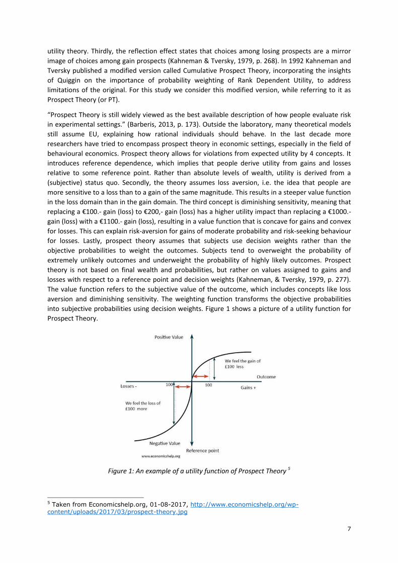
behavioural economics. Prospect theory allows for violations from expected utility by 4 concepts. It

introduces reference dependence, which implies that people derive utility from gains and losses

relative to some reference point. Rather than absolute levels of wealth, utility is derived from a

(subjective) status quo. Secondly, the theory assumes loss aversion, i.e. the idea that people are

more sensitive to a loss than to a gain of the same magnitude. This results in a steeper value function

in the loss domain than in the gain domain. The third concept is diminishing sensitivity, meaning that

replacing a €100.- gain (loss) to €200,- gain (loss) has a higher utility impact than replacing a €1000.-

gain (loss) with a €1100.- gain (loss), resulting in a value function that is concave for gains and convex

for losses. This can explain risk-aversion for gains of moderate probability and risk-seeking behaviour

for losses. Lastly, prospect theory assumes that subjects use decision weights rather than the

objective probabilities to weight the outcomes. Subjects tend to overweight the probability of

extremely unlikely outcomes and underweight the probability of highly likely outcomes. Prospect

theory is not based on final wealth and probabilities, but rather on values assigned to gains and

losses with respect to a reference point and decision weights (Kahneman, & Tversky, 1979, p. 277).

The value function refers to the subjective value of the outcome, which includes concepts like loss

aversion and diminishing sensitivity. The weighting function transforms the objective probabilities

into subjective probabilities using decision weights. Figure 1 shows a picture of a utility function for

Prospect Theory.

Figure 1: An example of a utility function of Prospect Theory 5

5 Taken from Economicshelp.org, 01-08-2017, http://www.economicshelp.org/wp-content/uploads/2017/03/prospect-theory.jpg

8

Barberis (2013) suggests that prospect theory can provide important explanations for insurance

markets where risk plays a crucial role. Throughout the literature on insurance, concave utility due to

expected utility and risk aversion is assumed (Wakker, 2008). As indicated before, empirically, a more

complex pattern has been found with risk aversion for moderate and high likelihood of gains and for

low likelihoods of losses, but with risk seeking for gains with low likelihood and for losses with

moderate or high likelihoods (Ibid). PT’s value function alone cannot explain why people gamble or

why people buy insurance. If people are generally risk-seeking for losses and risk-averse for gains,

then gambling and insurance should not have many customers. Decision weights, leading to

overweighting of unlikely and underweighting of likely probabilities, solves this problem.

Barberis (2013) gives an overview of the literature of Prospect Theory applied to insurance markets

and how reference-dependence plays a role in framing insurance. Sydnor (2010) explains why

individuals opt for a higher monthly premium, with a lower deductible even though the probability of

filing a claim is very low. Most people prefer to pay $100 a month more in premium than pay an

additional $500 in deductible more when filing a claim. Sydnor states that subjects overweight the

probability of filing a claim resulting in this violation of EU. It also depends on the reference point

taken. Köszegi and Rabin (2007) argue that the reference point is the expectation about future

outcomes, with the premium as an expected monthly expense. The deductible then only arises in the

event of a claim. Loss aversion is higher for this unexpected deductible than for the expected

premium. Therefore it is willing to pay a higher premium. Du, Feng and Hennessy (2014) find that

farmers in the United States of America do not optimise their crop insurance coverage according to

EU theory. Bougherara and Piet (2014) and Bocquého, Jacquet and Reynaud (2014) use show that

farmers’ decisions are better modelled using PT (as cited by Babcock, 2015). The reference point

taken to evaluate gains and losses is pivotal in explaining insurance decisions. According to Eckles

and Wise (2011) the reference point taken alters the value of insurance and the level of coverage

chosen. Brown (2008) argues that farmers do not take the reference point of expected wealth after

the insured event is realised, but rather see insurance as a stand-alone investment. The value of

insurance is then judged based on gains and losses in isolation from the effects of insurance on

overall income or consumption. Farmers thus frame insurance as a simple lottery rather than a risk

management tool. “A loss occurs when the premium paid is greater than the indemnity. A gain

occurs when the indemnity exceeds the premium paid.” (Babcock, 2015, p.1372).

Babcock tests how three different reference points explain the coverage level observed in American

crop-insurance decisions. The first reference point is initial wealth. According to Sydnor (2010) this

would lead to immediate losses when the premium is paid. Reynaud (2014) suggests that this may

explain low crop insurance in Europe. A second reference point is expected future wealth. As time

passes, the insurance premium is considered as sunk costs and are not included in the calculation of

expected wealth and thus of the reference point. A third reference point equals the costs of the

premium, framing insurance as a simple lottery. Babcock (2015) finds that this latter reference point

comes closest to explaining empirical crop insurance coverage decisions among American farmers.

Framing effects, the reference point taken, loss aversion and probability weighting are thus

subjective but important determinants for explaining insurance uptake. They might also play an

important role for crop-insurance uptake among subsistence farmers in Kenya. We now consider a

final alternative to non-expected utility provided by Andreoni and Sprenger.

2.4: Insurance contract design “Intertemporal decision-making involves a combination of certainty and uncertainty. The present is

known while the future is inherently risky.”(Andreoni & Sprenger, 2012, p. 3373). This is essentially

9

the reason why insurance exists. Andreoni and Sprenger follow the intuition of the certainty-effect of

the Allais paradox, to validate EU rather than refute it. As Andreoni and Sprenger indicate in their

paper, Allais already argued the same intuition in his 1953 paper Allais (1953, p. 530), that individuals

act as utility maximisers when 2 options are far from certainty, but when one option is certain and

the other uncertain, then a disproportionate preference for certainty prevails. Rather than throwing

EU out with the bathwater, Andreoni and Sprenger state that EU is only violated when certainty is

present. When it’s not present, subjects do follow the predictions of EU. They claim that this cannot

be explained by prospect theory or any other non-expected utility theories (Andreoni & Sprenger,

2012, p. 3358). Unsurprisingly, subjects strongly prefer certainty when its available. Most

interestingly, they find that when certainty is not present, so when there is no 100% payment option,

subjects’ behaviour closely mirrors the predictions of EU (Andreoni & Sprenger, 2012, p. 3359). They

argue that Prospect Theory’s probability weighting cannot account simultaneously for the

disproportionate preference of certainty when present with EU when far away from certainty.

The notion that people behave differently when there is a choice between a fully certain and an

uncertain option than if there are only uncertain options, deserves more attention. This could have

implications for insurance design as well, which we will examine in our experiments. This line of

thinking has been developed by Serfilippi et al. (2016) who test whether people that greatly value

certainty undervalue the benefits of insurance contracts. They test this this in a behavioural

experiment with farmers in Burkina Faso. Using choice lists with risky and degenerate lotteries, i.e.

lotteries with a probability of 1, they come up with a measure of Discontinuous Preferences of

Certainty (DPC). When subjects exhibit DPC, they overvalue the utility of a certain choice (or

degenerate lottery in PT) relative to uncertain choices. In this setting, the premium payment of

insurance policies is seen as a certain loss. It is hypothesised that this certain loss is overvalued by

DPC agents, claiming that if there are only uncertain options, there would be less deviations from

expected utility theory. They find that 30 percent of the farmers exhibit DPC. Next, they offer all

farmers two different designs of insurance contracts: a traditional insurance and one with a premium

rebate in bad years. The subjects have to indicate their WTP for both contracts. WTP for the DPC

farmers rose 30 percent for the rebate insurance, in contrast to no significant change in WTP for the

non-DPC subjects. The rationale is that the traditional insurance contract offers an option of

certainty, i.e. paying the premium in all states of the world, which is (negatively) overvalued by the

DPC-subjects. In contrast, in the rebate insurance design the certain loss is now a probable loss,

making it not fully certain. The argument is that without the certainty effect, subjects behave

according to EU. This affects those subjects who were relatively more sensitive to the certainty effect

and now that the certain loss of paying a premium is gone, exhibit significantly higher WTP for

insurance. A shortcoming of this research is that it does not incorporate basis risk in the experimental

design, which is arguable the most important source of uncertainty in index-insurances.

2.5 Synthesis and Hypotheses The literature review has shown that Prospect Theory is a promising theory of choice for our study as

it can explain the heterogeneity of behaviour towards risk and ambiguity. Probability weighting, loss

aversion, reference dependence, reflection and ambiguity attitudes all seem to play an important

role in explaining insurance purchasing decisions. Combining the literature on ambiguity attitudes

and prospect theory led us to construct the first three hypotheses 1-3. We subsequently provide a

synthesis of ambiguity, prospect theory and insurance design which resulted in hypotheses 4-6.

Our first hypothesis (1) is that ambiguity attitudes of Kenyan farmers will differ for gains and losses

and that the average farmer will be ambiguity averse for likely gains and unlikely losses and

10

ambiguity seeking for unlikely gains and likely losses. This is the pattern of ambiguity attitudes found

in the literature and we expect to find it as well in our sample. Our second hypothesis (2) is that a-

insensitivity will be higher for our sample than for samples from similar studies in Western countries.

A-insensitivity is the cognitive part and can be reduced through learning and experience. We expect

that the fact that our population has enjoyed less education and experience of probabilistic concepts

results in a higher estimate of a-insensitivity. Our third hypothesis (3) is that we expect Kenyan

subsistence farmers to be significantly loss averse. This means that they are more sensitive to a loss

than to a gain of the same magnitude.

For the elicitation of WTP for index insurance we follow the distinction in design made between a

traditional type of insurance and a rebate type of insurance. For the traditional type the payment of

the premium is certain in all states of the world and for the rebate-type of insurance subjects only

pay the premium if the harvest is good. In contrast to the design of Serfilippi et al (2016), we include

basis risk as an extra source of uncertainty to both the traditional and the rebate-type of insurance,

as this is considered one of the barriers to insurance uptake and we are interested in analysing the

effect of ambiguity attitudes have on WTP. The rebate-type does not reduce ambiguity, it increases

ambiguity and removes a state of certainty. It is actuarially equivalent to the traditional insurance

design. Assuming fully rational actors, there should thus be no difference in WTP for both designs.

However, Serfilippi et al. (2016) predict a higher WTP for the rebate insurance design for subjects

who are sensitive to certainty due to the disappearance of certainty. The idea being that they will

now behave according to EU. There are 2 important theoretical differences: our experiment has risk

and ambiguity and we do not measure sensitivity to certainty, but ambiguity attitudes and loss

aversion. Moreover, our participants will indicate their WTP for only 1 of the two designs, instead of

both designs. If we find evidence of our first hypothesis, than probabilistic sophistication is violated

and with it Expected Utility theory. This would mean that at least for index-insurance markets with its

inherent basis risk, Prospect Theory would be a better model for explaining decision-making under

ambiguity. With no ambiguity, and with no certainty, it is possible that EU still holds. This is outside

the scope of this research. More important is that we want to see whether the mechanism holds

merit: whether the removal of certainty increases the WTP for the rebate index insurance type and

which characteristics are related to this mechanism. This brings us to our final three hypotheses.

Our fourth hypothesis (4) states that ambiguity aversion and a-insensitivity are negatively correlated

to WTP for both index-insurance types due to basis risk; this relation is less strong for the rebate

type. Both insurance types include basis risk or ambiguity. We expect that ambiguity averse subjects

have a lower WTP for index an insurance design. Experiencing a bad harvest and not receiving a pay-

out is a highly unlikely loss and constitutes a worst-case scenario. This is exactly what pessimistic or

ambiguity averse subjects dislike and try to avoid. This is magnified for those individuals that are

more a-insensitive. A-insensitivity implies the overweighting of extreme probabilities. This overvalues

the probability of basis risk occurring and thus lowers WTP. For the rebate-type the payment of the

premium is also made uncertain, albeit only in a psychological way. If the premium is considered a

loss, it has changed from a certain to a probable loss. On average subjects are ambiguity seeking for

likely losses. This would result in a higher WTP for the rebate type, compared to the traditional type

that knows a certain loss of the premium payment. However, the worst-case scenario remains there,

of which the likelihood will be overweighted. Therefore ambiguity attitudes have a negative impact

on WTP for both designs due to basis risk. But the relation to the rebate type is less strong, due to

ambiguity-seeking tendencies for the premium payment.

Our fifth hypothesis (5) predicts that loss aversion is negatively correlated to WTP for the traditional

index insurance, assuming a stand-alone investment frame. The reference point taken to evaluate

11

gains and losses is pivotal in explaining insurance decisions. If farmers frame insurance as a simple

lottery, i.e. a stand-alone investment, as argued by Babcock (2015) and Brown (2008), the reference

point that signifies what constitutes a loss or a gain is the payment of the premium itself. A loss is

experienced whenever the premium paid exceeds the pay-out. For both designs, this is the case

when the harvest is good, or when the harvest is bad and the index is not triggered. Therefore, the

probability of a loss under this frame is large. Relatively more loss averse individuals will thus have

lower WTP for index insurance, if the stand-alone investment frame is assumed.

Our sixth and final hypothesis (6) states that WTP for the rebate-type insurance will be higher due to

a framing effect; this relation will be stronger for the relatively more loss averse. A difference in WTP

between two actuarially equivalent insurance designs could be explained by a change in frame that is

assumed when evaluating the insurance design. Serfilippi et al. (2016) argue that for the rebate type

insurance the certain loss is removed whose disutility was relatively overvalued. Thus making the

overall utility of the rebate scheme insurance higher for those subjects that overvalue certainty.

Another approach would be to say that the removal of certainty alters the reference-point

considered. Arguably, the rebate-type insurance does not entail an ‘investment’ as the payment of

the premium is made uncertain. Alternative frames through which insurance could be evaluated is

the initial wealth reference point or expected future wealth. The latter frame, which coincides with

the framework of Köszegi and Rabin (2007), equates the reference point with recent beliefs about

expected outcomes. As the rebate-type premium is deducted from the indemnity, the initial wealth

and expected outcome reference points are equivalent, but substantially higher than the stand-alone

investment reference point. Increasing the reference point, tends to increase the demand for

insurance (Babcock, 2015). The higher the reference point, the higher the probability and size of a

loss, resulting in a higher demand for insurance and thus a higher WTP. This effect is stronger among

the more loss averse.

In the following section we will explain how we will elicit ambiguity attitudes, measure loss aversion

and elicit WTP for the two insurance designs. We will also explain the design and procedure of our

experiments and how we will use the data of these experiments to test our hypotheses.

12

3. Experimental Design and Methodology In this section we give an overview of our sample and some descriptive statistics. We then present

the experimental design and procedure of our three games. In the first two games we test for

ambiguity attitudes and loss aversion. The loss aversion game followed the ambiguity game in a

digital survey using tablets. In the third game we elicit the WTP of farmers for different types of

insurance design using a framed lab-in-the-field experiment, meaning that it was a field experiment

in the context of being a maize farmer, which was the main crop cultivated in our sample. Whereas

the survey was presented to individual farmers, the WTP-game was played with a group of 8 to 14

farmers at the same time, depending on the size of the farmer group.

3.1: Sample The data used for this thesis comes from a study conducted in Kenya in May 2017. In total 276

female farmers belonging to 13 different farmer groups in Meru County participated in the

experiments. The 13 farmer groups selected have on average 20 members and have previously

participated in a study conducted from October 2016 till March 2017. Additional data used, comes

from this study that was conducted on in total 40 farmer groups. In October 2016, 19,9% of our

sample were insured as a result of a randomly awarded free insurance, conditional on the purchase

of certified improved seeds. The insurance type offered was a hybrid insurance: partially indemnity

and partially index based. APA Insurance is the Kenyan insurance company that provided this

insurance product. All subjects that did not participate in all three games, have been dropped from

the data. We also dropped all subjects that were not present during the March household survey. For

all remaining 276 subjects in this study, we have detailed information on individual, household and

farm characteristics. In our sample, 100% of the respondents is female, with an average age of 44.4

years and 6 years of education. Household size averages at 5.7 persons average income from farming

activities is 20592 Kenyan shilling (Ksh) a year.

Mobilisation was done by contacting the leaders of the farmer groups a week beforehand to set a

meeting date. Every day we would visit one or two farmer groups, preferably on their meeting day to

ensure a high turnout. The meeting place was often a primary school, a church, dispensary or an

open field. We brought chairs for the WTP-game, so the subjects could sit comfortably.

Randomisation was done by stratified sampling at the group level. Once everyone had arrived, we

assigned the different groups. Farmers were randomly given a tag which said either I0-L, I0-G, I1-L or

I1-G. ‘I0’ and ‘I1’ represent the assigned insurance design for the WTP-game, respectively the

traditional type of index-insurance (I0) or the rebate type (I1). The ‘–G’ or ‘–L’ stands for the ‘Gain’ or

‘Lose’ scenario in the ambiguity game.

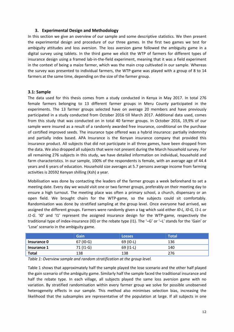
Gain Losses Total

Insurance 0 67 (I0-G) 69 (I0-L) 136

Insurance 1 71 (I1-G) 69 (I1-L) 140

Total 138 138 276

Table 1: Overview sample and random stratification at the group level.

Table 1 shows that approximately half the sample played the lose scenario and the other half played

the gain scenario of the ambiguity game. Similarly half the sample faced the traditional insurance and

half the rebate type. In each village, all subjects played the same loss aversion game with no

variation. By stratified randomisation within every farmer group we solve for possible unobserved

heterogeneity effects in our sample. This method also minimises selection bias, increasing the

likelihood that the subsamples are representative of the population at large. If all subjects in one

13

village would play the same game, village-specific unobserved variables might influence the results.

For example some villages have more experience with insurance, are less poor, are more remote

than other villages. By randomly stratifying in every farmer group, we control for those unobserved

differences between the villages. The type of insurance design that would start was alternated every

farmer group. The insurance type that did not start, would first do the survey module containing the

ambiguity and loss aversion game.

Nine experienced enumerators, who were also part of the household surveys in October and March,

explained the experimental protocols in Kimeru or Kiswahili and made sure the farmers were able to

understand the games.6 Four of them were exclusively trained in the WTP-game, two for each type of

insurance design. To avoid mistakes, the enumerators only presented one type of insurance design.

The other five enumerators conducted the survey module. Once the first round was over, the groups

switched. Farmers were instructed not to talk to each other to reduce information spill-over effects

from one group to another. The enumerators were monitoring this and would fine subjects when

disclosing information to one another. One round lasted approximately 45 minutes to an hour. In

total the experiments took around 2 to 2 and a half hours depending on the farmer group size.

3.2: Incentives Every subject plays 3 games, (1) the ambiguity game, (2) the loss aversion game and (3) the WTP-

game. For every game money can be won dependent on their choices during the game and on luck.

The participant received a voucher with the amount won for every game. Once all three games were

completed, the vouchers were collected, put in a large jug and one of the vouchers was randomly

selected which was paid out in cash to the subject.

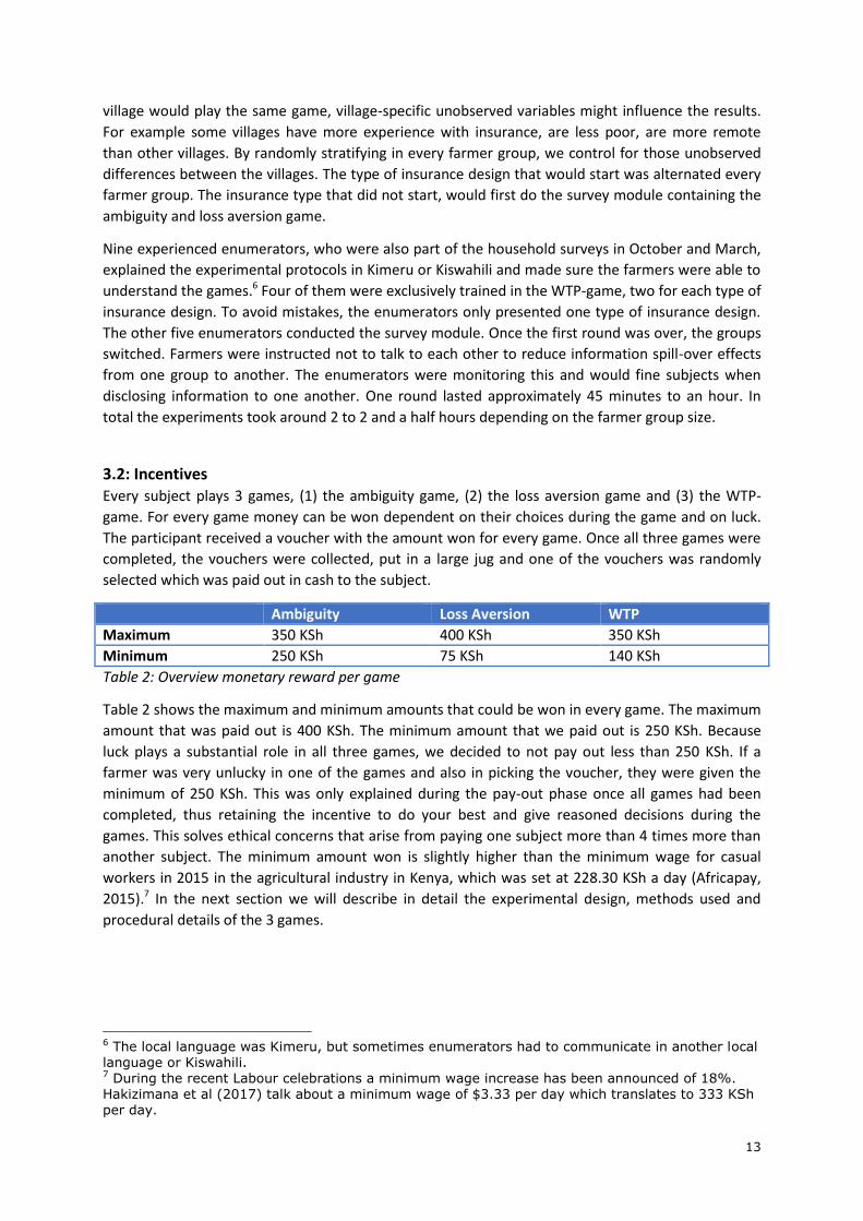
Ambiguity Loss Aversion WTP

Maximum 350 KSh 400 KSh 350 KSh

Minimum 250 KSh 75 KSh 140 KSh

Table 2: Overview monetary reward per game

Table 2 shows the maximum and minimum amounts that could be won in every game. The maximum

amount that was paid out is 400 KSh. The minimum amount that we paid out is 250 KSh. Because

luck plays a substantial role in all three games, we decided to not pay out less than 250 KSh. If a

farmer was very unlucky in one of the games and also in picking the voucher, they were given the

minimum of 250 KSh. This was only explained during the pay-out phase once all games had been

completed, thus retaining the incentive to do your best and give reasoned decisions during the

games. This solves ethical concerns that arise from paying one subject more than 4 times more than

another subject. The minimum amount won is slightly higher than the minimum wage for casual

workers in 2015 in the agricultural industry in Kenya, which was set at 228.30 KSh a day (Africapay,

2015).7 In the next section we will describe in detail the experimental design, methods used and

procedural details of the 3 games.

6 The local language was Kimeru, but sometimes enumerators had to communicate in another local language or Kiswahili. 7 During the recent Labour celebrations a minimum wage increase has been announced of 18%. Hakizimana et al (2017) talk about a minimum wage of $3.33 per day which translates to 333 KSh per day.

14

3.3: Game 1: Measuring Ambiguity Attitudes As we analysed in the theoretical framework, ambiguity attitudes consist of ambiguity aversion and

ambiguity generated likelihood insensitivity. The ambiguity game captures both concepts and is

based on the methodology of Dimmock et al. (2015 and 2016). This method has been used in large

household surveys and in lab experiments. The method has been slightly adjusted to ensure better

understanding for the population under study. The ambiguity game uses 3 scenarios and subsequent

variations on every scenario to estimate the ambiguity attitudes. We offered respondents real

monetary rewards based on one of their choices in one of the scenarios. Half of the subjects played

an ambiguity game where they could win 100 KSh, the other half could lose 100 KSh. To even out the

average winnings of both groups, gain-participants received a participation fee of 250 KSh and lose-

participants 350 KSh. Every participant could therefore finish the game with either 250 or 350 KSh.

The questions in our survey were similar to those in the famous Ellsberg experiment (1961). Rather

than two urns with balls of 2 colours, we ask respondents to choose between an unambiguous box

(box 1) and an ambiguous box (box 2).8 Because we could not bring computers with internet access

into the field, we used non-transparent lunchboxes with coloured beads instead.9 Each box holds

exactly 100 beads, The respondents were asked to choose one of the boxes to draw a bead from. If

this bead was the winning colour, they would win 100 KSh. The contents of box 1 were known and

shown to the participant. The contents of box 2 were unknown and hence ambiguous. The

respondents only knew the amount of beads and how many different colours could be present in the

ambiguous box. Besides stating a preference, respondents could also state to find both boxes

‘equally attractive’ which is the same as ‘indifference’ in Dimmock’s terminology.10 In scenario 2 and

3 the amount of beads remains 100, but instead of only 2 colours, the boxes contain beads of 10

different colours to simulate situations of high or low likelihood. We will first explain the procedures

of the game for the gain scenarios. Then we explain how ambiguity indices can be constructed from

the results of the game. Finally we show how the game was set up for the lose scenario.

Elicitation Procedure

In the first scenario, as depicted in figure 2, box 1 contains 50 green and 50 yellow beads. Box 2

contains 100 beads of either green or yellow colour with an unknown composition. The participant

wins if a green bead is drawn. There could be between 0 and 100 green beads in box 2. Following

Dimmock et al. (2015), Baillon and Bleichrodt (2015), Baillon et al. (2015) and many others writing on

ambiguity, we employ matching probabilities to estimate ambiguity attitudes. A matching probability

(m) is the objective probability for which an agent is indifferent between the risky option and the

ambiguous option. For our game this means that m is the indifference between winning 100 KSh

under the ambiguous option (box 2) and winning 100 KSh with probability m for the risky option (box

1). We elicited m using a sequence of questions, while changing the colour ratio of beads in box 1, for

which the respondent had to state their choice: box 1, box 2, or equally attractive.

In theory it is possible that a non-neutral response to the first round of scenario 1, can be reconciled

with subjective expected utility theory if the subject assigned a very low subjective probability to

drawing a green bead from box 2. Abdellaoui et al. (2011) and Dimmock et al. (2016) therefore give

subjects the opportunity to alter the winning colour in box 2. They find that less than 2 percent of the

respondents changed the winning colour in box 2. Dimmock et al. (2015) also test this by allowing

respondents to choose the winning colour of the whole game. Fewer than 1 percent opted for this.

8 Dimmock et al use box K for the known box, and box U for the unknown or ambiguous box. 9 We used the small coloured beads that are famously used for Kenyan jewellery. 10 We named this option equally attractive, to reduce any negative connotations of disinterest from the respondents, indifference might imply when translating to Kimeru.

15

All three studies show that people are indifferent about the winning colour and there were no

significant differences in the mean matching probabilities of the group that was allowed to switch

colour and the group that could not switch. We therefore did not allow respondents to change the

winning colour.

If the respondent’s response was ‘equally attractive’, the survey continued with the second scenario.

If the respondent indicated that box 1 was preferred, then the enumerator replaced some of the

green beads with yellow beads, reducing the known winning probability of box 1. If the respondent

indicated that box 2 was preferred, then some of the yellow beads of box 1 were replaced by green

beads, increasing the observable winning probability of box 1. Whenever the subject selects box 1,

this box is made less attractive. Whenever the subject selects box 2, box 1 is made more attractive.

The content of box 2 were never changed, never visible and remained ambiguous throughout.

Changing the ratio of beads was done by method of bisection as explained in the annex of Dimmock

et al. (2016). After every choice, the difference between the lower bound and the upper round on

the matching probability is reduced by half. This would continue until the answer ‘equally attractive’

was given or until a maximum of three additional rounds. After the final round, the matching

probability is the objective probability of box 1 if the respondent answered equally attractive,

otherwise the midpoint of the average of the lower and upper bound of the final round is taken.

Figure 2: Starting scenario 1 of Ambiguity game (Gain)

Estimating Ambiguity Aversion

Subjects that find both boxes equally attractive in the first round, where the objective probability of

winning in box 1 is 50%, are ambiguity neutral. This means that the respondent treats the ambiguous

box (2) as having the same percentage of winning as the known box (1), i.e. 50% chance of drawing a

green bead. Hence the matching probability m is 0.5. If the respondent preferred box 1 over box 2,

then the respondent is ambiguity averse with m < 0.5. Respondents that choose box 2 over box 1 in

the first round are ambiguity seeking with m > 0.5.

The literature on ambiguity predicts that ambiguity aversion is dependent on the likelihood of the

event. Dimmock et al. (2016) give proof in a large representative household sample that people

respond differently to situations if the likelihood of winning is 50-50, very high or very low. On

average people are average ambiguity seeking for low likelihoods and ambiguity averse for high

likelihoods of winning. We therefore include a scenario with a low likelihood and one with a high

likelihood of winning. Other methods to estimate ambiguity attitudes like Baillon & Bleichrodt

(2015), employ a similar strategy. Our second scenario has a very low likelihood of winning in the

16

starting scenario, i.e. 10%, whereas the third scenario has a very high likelihood of winning, i.e. 90%.

Both the second and the third scenario are played with 100 beads of 10 different colours.

For the second scenario, In box 1, there are 10 beads of every colour and 100 beads in total. The

respondent wins if a green bead is drawn from the box, thus giving a winning chance of 10%. If any

colour other than green was drawn, the respondent would not win. After every choice of the

respondent, the composition of the beads in box 1 would be altered using the same method of

bisection. For the third scenario, the starting situation is the same as the second scenario, but the

winning condition is different. Now, the respondent wins if the bead drawn is NOT green, resulting in

a 90% winning probability. Similarly, after every choice, the composition of the beads in box 1 is

rearranged using the method of bisection until the matching probability is found. The second and

third scenario provides us with information on whether ambiguity aversion is dependent on

likelihood. Together with the matching probability of scenario 1, we can construct indices of

ambiguity aversion for moderate, very low and very high likelihoods of winning. The indices that are

used in this study are calculated as follows.

We will denote 𝐴𝐴50+ as the ambiguity aversion index for the first Gain scenario where the

objective winning probability p of box 1 in the starting situation of scenario 1 was 50%. Likewise, we

let 𝐴𝐴10+refer to the ambiguity aversion index for scenario 2, and 𝐴𝐴90+ for scenario 3. The index

is calculated by deducting the matching probability from the objective winning probability of box 1 in

the first round of the scenario: 𝐴𝐴+ = 𝑝 − 𝑚. This leads to the following ambiguity aversion indices:

𝐴𝐴50+ = 50% − 𝑚50

𝐴𝐴10+ = 10% − 𝑚10

𝐴𝐴90+ = 90% − 𝑚90

Positive values of 𝐴𝐴+imply ambiguity aversion. Negative values imply ambiguity seeking and 𝐴𝐴+=0

signifies ambiguity neutrality.

Check questions and Pay-Out

After the three scenarios were answered, the survey included 2 check questions to test whether the

participants behave consistently. The matching probability of the first scenario was taken as a

starting point. For m = 0.5, the respondent was indifferent between box 1 and box 2, with an

objective winning percentage 50% for box 1. The check questions take the matching probability of

the first scenario and do this -10 and +10 winning beads. In our example, the first check question

recreates scenario 1 with 40 winning beads for the first question and 60 winning beads for the

second question. For the first question, to be logically consistent, the respondent should answer that

box 2 is preferred, for the second question box 1 should be preferred. These questions will be

important for analysing whether the respondents understood the game and behave consistently.

After answering the sequence of questions for all three scenarios, the tablet would randomly select

one of the three scenarios to be played out for real. This meant that after having selected one of the

three scenario’s, one of the situations answered by the respondent was randomly selected. The

respondent would win if the bead had the winning colour. If the respondent’s answer was box 1,

then the selected situation was recreated from which a bead was drawn. If the respondent said box

2, then the respondent would draw a bead from box 2. If a situation was selected that was answered

with equally attractive, then the enumerator would let the respondent draw a bead from box 1.11

11 If the respondent did not agree with this, the enumerator could also select a bead from box 2.

17

Estimating A-insensitivity

The second component of ambiguity attitudes is a-insensitivity or ambiguity generated likelihood

insensitivity. A-insensitivity is a measure of how well one distinguishes between changes in likelihood

or whether one perceives ambiguous likelihoods as mostly 50-50 situations. Theory predicts that

people overweight the probability of highly unlikely events and underweight the probability of highly

likely events to occur. The second and third scenario provides us with information on how sensitive

farmers are to different likelihoods. We can construct the following A-insensitivity index. We use the

ambiguity aversion index for the second and third scenario. The objective winning probabilities of

scenario 2 and 3 add to 100%. They are composite events, meaning that also the matching

probabilities should add to 1 if completely neutral and rational. We can thus measure a-insensitivity :

𝐴𝐼+ = 𝐴𝐴90+ − 𝐴𝐴10+

Positive values of 𝐴𝐼+mean that the subject is a-insensitive. Negative values signify a-oversensitivity.

Neutral respondents have ambiguity indices of 0 and their measure of 𝐴𝐼+will therefore also be

equal to 0.

Ambiguity attitudes for Losses

Half of the sample played the ambiguity game with the prospect of losing 100 KSh. Their participation

fee was higher to encompass a possible loss. The aim is to determine whether ambiguity attitudes for

prospective losses are different from prospective gains. The three scenarios remain exactly the same.

Only the winning condition changes from ‘win’ to ‘lose’. Hence where one could win if a green bead

is drawn, in scenario 1 and 2, now the respondents lose if a green bead is drawn. Consequently, for

scenario 3, one loses if a green bead is NOT drawn, meaning that for every other colour than green,

one loses. This translates into objective losing probabilities for box 1 of 50%, 10% and 90% for the

three scenarios. The ambiguity indices for losses are constructed as follows:

𝐴𝐴50− = 𝑚50 − 50%

𝐴𝐴10− = 𝑚10 − 10%

𝐴𝐴90− = 𝑚90 − 90%

Similar to that the ambiguity index for aversion is a reversal of the one for gains (𝐴𝐴50+= 50% -

𝑚50). The a-insensitivity index for losses is also reversed.

𝐴𝐼− = 𝐴𝐴10− − 𝐴𝐴90−

In the second losing scenario 𝐴𝐴10−, there is actually a not losing probability of 90%. Similarly the

third scenario, there is a not losing probability of 10%. So the second scenario has the same winning

probability as the third gain scenario, and the third losing has the same as the second gain scenario.

If we want to measure insensitivity to likelihood for losses, or the tendency to reduce probabilities to

50-50 scenarios, we need to adjust the equation accordingly.

Practicalities

In previous studies, these experiments have mainly been conducted with university students or in a

general survey on the American population. This is the first time that such an abstract experiment is

done on a population that is arguably less educated and less exposed to probabilistic concepts in

daily life. Most respondents are poor female farmers with little education or even illiterate. We

therefore tried to keep the experiment as simple and visual as possible. Enumerator followed a fixed

script on the tablet reiterating every round the winning/losing condition, the amount of beads of

every colour in box 1, the amount of beads in box 2 and changes in the ratio of beads in box 1. The

actual content of box 1 throughout the various rounds was visualised on a white plastic plate. There

the enumerators recreated the constellation of the coloured beads in play at the moment so that the

18

respondent could clearly see the colours in play. If it was still not clear to the farmer, the enumerator

had a picture of every possible situation on their tablet, that they would show to the farmer. It was

not uncommon that an enumerator explained the game multiple times before the respondent

understood the game.

The lunchboxes with beads were checked every night and given to another enumerator the next day

to minimise enumerators’ knowledge of the contents of the ambiguous boxes. Every 4 days, we

removed all the beads from the boxes and randomly filled the ambiguous boxes with beads. We used

two big jugs to fill with green/yellow beads and beads of ten different colours. After shaking the jugs,

we poured the beads into the ambiguous boxes until the exact amount of 100 beads. In total there

were 3 boxes per enumerator. One box 1, and two times a box 2. One ambiguous box for scenario 1

and one ambiguous box for scenario 2 and three.

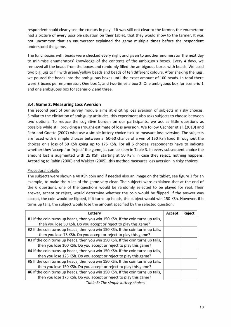
3.4: Game 2: Measuring Loss Aversion The second part of our survey module aims at eliciting loss aversion of subjects in risky choices.

Similar to the elicitation of ambiguity attitudes, this experiment also asks subjects to choose between

two options. To reduce the cognitive burden on our participants, we ask as little questions as

possible while still providing a (rough) estimate of loss aversion. We follow Gächter et al. (2010) and

Fehr and Goette (2007) who use a simple lottery choice task to measure loss aversion. The subjects

are faced with 6 simple choices between a 50-50 chance of a win of 150 KSh fixed throughout the

choices or a loss of 50 KSh going up to 175 KSh. For all 6 choices, respondents have to indicate

whether they ‘accept’ or ‘reject’ the game, as can be seen in Table 3. In every subsequent choice the

amount lost is augmented with 25 KSh, starting at 50 KSh. In case they reject, nothing happens.

According to Rabin (2000) and Wakker (2005), this method measures loss aversion in risky choices.

Procedural details

The subjects were shown a 40 KSh coin and if needed also an image on the tablet, see figure 3 for an

example, to make the rules of the game very clear. The subjects were explained that at the end of

the 6 questions, one of the questions would be randomly selected to be played for real. Their

answer, accept or reject, would determine whether the coin would be flipped. If the answer was

accept, the coin would be flipped, if it turns up heads, the subject would win 150 KSh. However, if it

turns up tails, the subject would lose the amount specified by the selected question.

Lottery Accept Reject

#1 If the coin turns up heads, then you win 150 KSh. If the coin turns up tails, then you lose 50 KSh. Do you accept or reject to play this game?

#2 If the coin turns up heads, then you win 150 KSh. If the coin turns up tails, then you lose 75 KSh. Do you accept or reject to play this game?

#3 If the coin turns up heads, then you win 150 KSh. If the coin turns up tails, then you lose 100 KSh. Do you accept or reject to play this game?

#4 If the coin turns up heads, then you win 150 KSh. If the coin turns up tails, then you lose 125 KSh. Do you accept or reject to play this game?

#5 If the coin turns up heads, then you win 150 KSh. If the coin turns up tails, then you lose 150 KSh. Do you accept or reject to play this game?

#6 If the coin turns up heads, then you win 150 KSh. If the coin turns up tails, then you lose 175 KSh. Do you accept or reject to play this game?

Table 3: The simple lottery choices

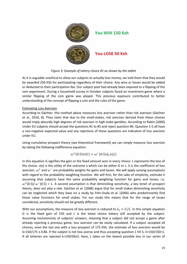
19

Figure 3: Example of lottery choice #1 as shown by the tablet

As it is arguable unethical to allow our subjects to actually lose money, we told them that they would

be awarded 250 KSh for participating regardless of their choice. Any wins or losses would be added

or deducted to their participation fee. Our subject pool had already been exposed to a flipping of the

coin experiment. During a household survey in October subjects faced an investment game where a

similar flipping of the coin game was played. This previous exposure contributed to better

understanding of the concept of flipping a coin and the rules of the game.

Estimating Loss Aversion

According to Gächter, this method above measures loss aversion rather than risk aversion (Gächter

et al., 2010, 8). They claim that due to the small-stakes, risk aversion derived from these choices

would imply absurdly high degrees of risk aversion in high-stake gambles. According to Rabin (2000)

Under EU subjects should accept the questions #1 to #5 and reject question #6. Question 1-5 all have

a non-negative expected value and any rejections of these questions are indicative of loss aversion

under EU.

Using cumulative prospect theory (see theoretical framework) we can simply measure loss aversion

by taking the following indifference equation:

𝜔+(0.5)𝑣(𝐺) = 𝜔−(0.5)𝜆1𝑣(𝐿)

In this equation G signifies the gain or the fixed amount won in every choice. L represents the loss of

the choice. v(x) is the utility of the outcome x which can be either G or L. λ is the coefficient of loss

aversion. 𝜔+ and 𝜔− are probability weights for gains and losses. We will apply varying assumptions

with regard to the probability weighting function. We will first, for the sake of simplicity, estimate λ

assuming that subjects have the same probability weighting function for gains and losses, i.e.

𝜔+(0.5)/ 𝜔−(0.5) = 1. A second assumption is that diminishing sensitivity, a key tenet of prospect

theory, does not play a role. Gächter et al. (2008) argue that for small stakes diminishing sensitivity

can be neglected which they base on a study by Fehr-Duda et al. (2006) who predominantly find

linear value functions for small stakes. For our study this means that for the range of losses

considered, sensitivity should not be greatly different.

With our assumptions, the measure of loss aversion is reduced to 𝜆1 = 𝐺/𝐿. In this simple equation

G is the fixed gain of 150 and L is the latest choice lottery still accepted by the subject.

Assuming monotonicity of subjects’ answers, meaning that a subject did not accept a game after

already rejecting a previous game, loss aversion can be easily calculated. If a subject accepted all

choices, even the last one with a loss prospect of 175 KSh, the estimate of loss aversion would be

λ=150/175 ≤ 0.86. If the subject is not loss averse and thus accepting question 1 till 5, λ=150/150=1.

If all lotteries are rejected λ=150/50≥3. Here, L takes on the lowest possible loss in our series of

20

choices even though this was not accepted. This makes the loss aversion coefficient greater or equal

to 3. Using this method, loss aversion can be estimated for individuals.

Stricter assumptions

We will also estimate loss aversion taking reasonable estimates of probability weights and

diminishing sensitivity from the literature. Booij and van de Kuilen (2009) give an overview of the

literature on the parameters for the probability weighting function and the value function since the

original paper of Kahneman and Tversky. They also give their own estimates based on a study

conducted on a representative sample of the general public of N=1,935. Following Gächter et al.

(2010), we can include some of PT’s assumption to get a better estimate λ, giving us the following

equations:

𝜆 = 𝜔 ∗ (𝐺𝛼

𝐿𝛽)

𝜔 ≡ 𝜔+(0.5)/𝜔−(0.5).

In this equation α and β represent diminishing sensitivity for gains and losses respectively and ω

represents probability weighting for gains and losses. Gächter et al. (2010) take ω=0.86, based on a

study by Abdellaoui (2000), which is the largest difference between probability weighting for gains

and losses that they could find in the literature. The probability weighting function is often described

by two properties: sensitivity towards probabilities and pessimism, which give it the elevated inverse-

S shape (Booij and van de Kuilen, 2009). Assuming Prospect Theory rather than a Multiple Prior

model, this is essentially what we capture in our ambiguity game. As we expect to find strong

pessimism and likelihood insensitivity, stronger than in most samples on Western populations, it

seems appropriate to take the estimate ω=0.86 of Abdellaoui (2000). Tversky and Kahneman (1992)

estimated ω=0.933 and Booij and Van de Kuilen (2009) find ω=0.966. For diminishing sensitivity

Gächter et al. take α=0.95 and β=0.92, following Booij and van de Kuilen (2007). In a review of all

estimates of Prospect Theory’s parameters Booij and Van de Kuilen, report that most

contemporaneous studies find diminishing sensitivity parameters to lie between 0.8 and 1 (2009).

Themselves they find, using maximum likelihood estimation, α=0.859 and β=0.826, whereas Tversky

and Kahneman (1992) reported α=β=0.88. In a second estimation of loss aversion we therefore take

ω=0.86 and α=0.859 and β=0.826 to be reasonable estimates for our study, giving us the following

equation:

𝜆2 = 0.86 ∗ (𝐺0.859

𝐿0.826 )

Finally, we will try to estimate loss aversion using the results of the ambiguity game to estimate the

parameters of the probability weighting function. According to Booij and Van de Kuilen (2009), the

most commonly used specification is Goldstein and Einhorn’s (1987) linear-in-log-odds specification,

which is noted as:

𝜔(𝑝) =𝛿𝑝𝛾

𝛿𝑝𝛾 + (1 − 𝑝)𝛾

In this equation δ represents pessimism, or the elevation of the intercept away from 0 of the value

function. This is captured by our estimate of ambiguity aversion of the first scenario of the ambiguity

game for gains and losses. 𝛾 represents the curvature of probability weighting function, resulting in

its inverse-S shape. This we essentially capture with our estimate of a-insensitivity, which is derived

from the second and third scenario of the ambiguity game. Assuming 𝜔 ≡ 𝜔+(0.5)/𝜔−(0.5), we

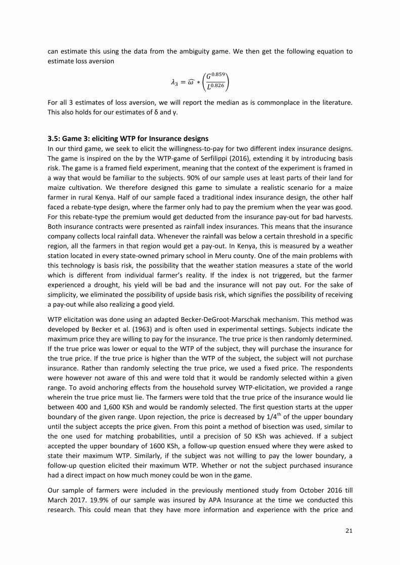
21

can estimate this using the data from the ambiguity game. We then get the following equation to

estimate loss aversion

𝜆3 = 𝜔 ̂ ∗ (𝐺0.859

𝐿0.826 )

For all 3 estimates of loss aversion, we will report the median as is commonplace in the literature.

This also holds for our estimates of δ and γ.

3.5: Game 3: eliciting WTP for Insurance designs In our third game, we seek to elicit the willingness-to-pay for two different index insurance designs.

The game is inspired on the by the WTP-game of Serfilippi (2016), extending it by introducing basis

risk. The game is a framed field experiment, meaning that the context of the experiment is framed in

a way that would be familiar to the subjects. 90% of our sample uses at least parts of their land for

maize cultivation. We therefore designed this game to simulate a realistic scenario for a maize

farmer in rural Kenya. Half of our sample faced a traditional index insurance design, the other half

faced a rebate-type design, where the farmer only had to pay the premium when the year was good.

For this rebate-type the premium would get deducted from the insurance pay-out for bad harvests.

Both insurance contracts were presented as rainfall index insurances. This means that the insurance

company collects local rainfall data. Whenever the rainfall was below a certain threshold in a specific

region, all the farmers in that region would get a pay-out. In Kenya, this is measured by a weather

station located in every state-owned primary school in Meru county. One of the main problems with

this technology is basis risk, the possibility that the weather station measures a state of the world

which is different from individual farmer’s reality. If the index is not triggered, but the farmer

experienced a drought, his yield will be bad and the insurance will not pay out. For the sake of

simplicity, we eliminated the possibility of upside basis risk, which signifies the possibility of receiving

a pay-out while also realizing a good yield.

WTP elicitation was done using an adapted Becker-DeGroot-Marschak mechanism. This method was

developed by Becker et al. (1963) and is often used in experimental settings. Subjects indicate the

maximum price they are willing to pay for the insurance. The true price is then randomly determined.

If the true price was lower or equal to the WTP of the subject, they will purchase the insurance for

the true price. If the true price is higher than the WTP of the subject, the subject will not purchase

insurance. Rather than randomly selecting the true price, we used a fixed price. The respondents

were however not aware of this and were told that it would be randomly selected within a given

range. To avoid anchoring effects from the household survey WTP-elicitation, we provided a range

wherein the true price must lie. The farmers were told that the true price of the insurance would lie

between 400 and 1,600 KSh and would be randomly selected. The first question starts at the upper

boundary of the given range. Upon rejection, the price is decreased by 1/4th of the upper boundary

until the subject accepts the price given. From this point a method of bisection was used, similar to

the one used for matching probabilities, until a precision of 50 KSh was achieved. If a subject

accepted the upper boundary of 1600 KSh, a follow-up question ensued where they were asked to

state their maximum WTP. Similarly, if the subject was not willing to pay the lower boundary, a

follow-up question elicited their maximum WTP. Whether or not the subject purchased insurance

had a direct impact on how much money could be won in the game.

Our sample of farmers were included in the previously mentioned study from October 2016 till

March 2017. 19.9% of our sample was insured by APA Insurance at the time we conducted this

research. This could mean that they have more information and experience with the price and

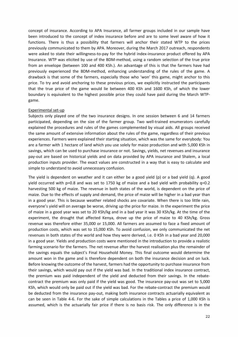
22

concept of insurance. According to APA Insurance, all farmer groups included in our sample have

been introduced to the concept of index insurance before and are to some level aware of how it

functions. There is thus a possibility that farmers will anchor their stated WTP to the prices

previously communicated to them by APA. Moreover, during the March 2017 outreach, respondents

were asked to state their willingness-to-pay for the hybrid index-insurance product offered by APA

Insurance. WTP was elicited by use of the BDM-method, using a random selection of the true price

from an envelope (between 100 and 400 KSh.). An advantage of this is that the farmers have had

previously experienced the BDM-method, enhancing understanding of the rules of the game. A

drawback is that some of the farmers, especially those who ‘won’ this game, might anchor to this

price. To try and avoid anchoring to these previous prices, we explicitly instructed the participants

that the true price of the game would lie between 400 KSh and 1600 KSh, of which the lower

boundary is equivalent to the highest possible price they could have paid during the March WTP-

game.

Experimental set-up

Subjects only played one of the two insurance designs. In one session between 6 and 14 farmers

participated, depending on the size of the farmer group. Two well-trained enumerators carefully

explained the procedures and rules of the games complemented by visual aids. All groups received

the same amount of extensive information about the rules of the game, regardless of their previous

experiences. Farmers were explained their starting situation, which was the same for everybody: You

are a farmer with 1 hectare of land which you use solely for maize production and with 5,000 KSh in

savings, which can be used to purchase insurance or not. Savings, yields, net revenues and insurance

pay-out are based on historical yields and on data provided by APA insurance and Shalem, a local

production inputs provider. The exact values are constructed in a way that is easy to calculate and

simple to understand to avoid unnecessary confusion.

The yield is dependent on weather and it can either be a good yield (p) or a bad yield (q). A good

yield occurred with p=0.8 and was set to 1750 kg of maize and a bad yield with probability q=0.2

harvesting 500 kg of maize. The revenue in both states of the world, is dependent on the price of

maize. Due to the effects of supply and demand, the price of maize will be higher in a bad year than

in a good year. This is because weather related shocks are covariate. When there is too little rain,

everyone’s yield will on average be worse, driving up the price for maize. In the experiment the price

of maize in a good year was set to 20 KSh/kg and in a bad year it was 30 KSh/kg. At the time of the

experiment, the drought that affected Kenya, drove up the price of maize to 40 KSh/kg. Gross

revenue was therefore either 35,000 or 15,000. All farmers are assumed to face a fixed amount of

production costs, which was set to 15,000 KSh. To avoid confusion, we only communicated the net

revenues in both states of the world and how they were derived, i.e. 0 KSh in a bad year and 20,000

in a good year. Yields and production costs were mentioned in the introduction to provide a realistic

farming scenario for the farmers. The net revenue after the harvest realisation plus the remainder of

the savings equals the subject’s Final Household Money. This final outcome would determine the

amount won in the game and is therefore dependent on both the insurance decision and on luck.

Before knowing the outcome of the harvest, farmers had the opportunity to purchase insurance from

their savings, which would pay out if the yield was bad. In the traditional index insurance contract,

the premium was paid independent of the yield and deducted from their savings. In the rebate-

contract the premium was only paid if the yield was good. The insurance pay-out was set to 5,000

KSh, which would only be paid out if the yield was bad. For the rebate-contract the premium would

be deducted from the insurance pay-out, making both insurance contracts actuarially equivalent as

can be seen in Table 4-6. For the sake of simple calculations in the Tables a price of 1,000 KSh is

assumed, which is the actuarially fair price if there is no basis risk. The only difference is in the

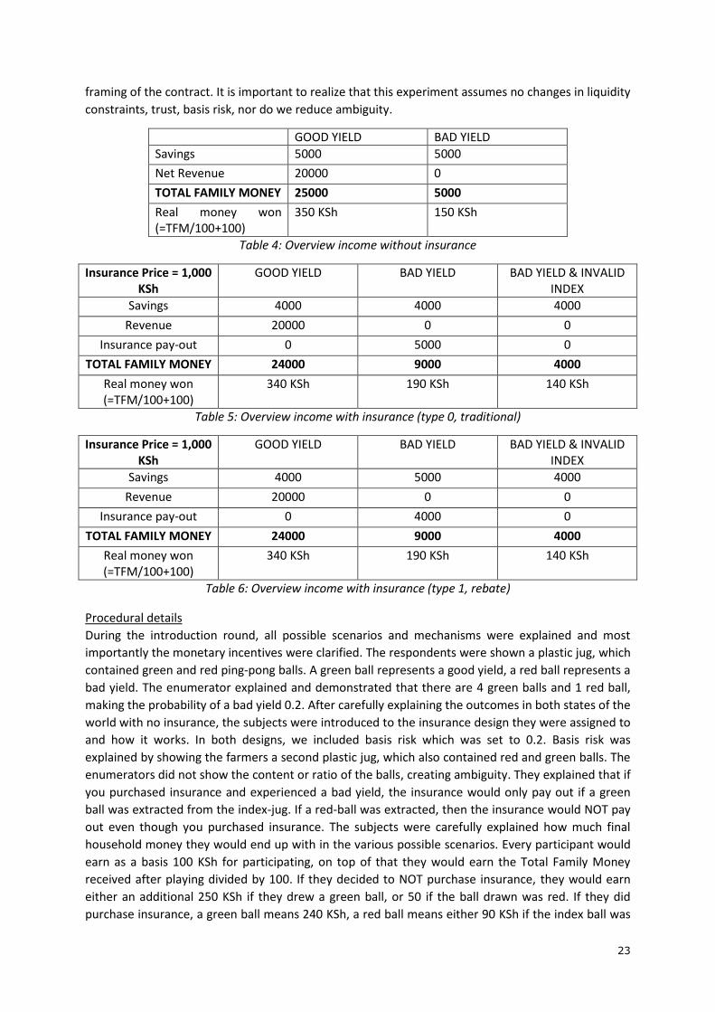
23

framing of the contract. It is important to realize that this experiment assumes no changes in liquidity

constraints, trust, basis risk, nor do we reduce ambiguity.

GOOD YIELD BAD YIELD

Savings 5000 5000

Net Revenue 20000 0

TOTAL FAMILY MONEY 25000 5000

Real money won (=TFM/100+100)

350 KSh 150 KSh

Table 4: Overview income without insurance

Insurance Price = 1,000 KSh

GOOD YIELD BAD YIELD BAD YIELD & INVALID INDEX

Savings 4000 4000 4000

Revenue 20000 0 0

Insurance pay-out 0 5000 0

TOTAL FAMILY MONEY 24000 9000 4000

Real money won (=TFM/100+100)

340 KSh 190 KSh 140 KSh

Table 5: Overview income with insurance (type 0, traditional)

Insurance Price = 1,000 KSh

GOOD YIELD BAD YIELD BAD YIELD & INVALID INDEX

Savings 4000 5000 4000

Revenue 20000 0 0

Insurance pay-out 0 4000 0

TOTAL FAMILY MONEY 24000 9000 4000

Real money won (=TFM/100+100)

340 KSh 190 KSh 140 KSh

Table 6: Overview income with insurance (type 1, rebate)

Procedural details

During the introduction round, all possible scenarios and mechanisms were explained and most

importantly the monetary incentives were clarified. The respondents were shown a plastic jug, which

contained green and red ping-pong balls. A green ball represents a good yield, a red ball represents a

bad yield. The enumerator explained and demonstrated that there are 4 green balls and 1 red ball,

making the probability of a bad yield 0.2. After carefully explaining the outcomes in both states of the

world with no insurance, the subjects were introduced to the insurance design they were assigned to

and how it works. In both designs, we included basis risk which was set to 0.2. Basis risk was

explained by showing the farmers a second plastic jug, which also contained red and green balls. The

enumerators did not show the content or ratio of the balls, creating ambiguity. They explained that if

you purchased insurance and experienced a bad yield, the insurance would only pay out if a green

ball was extracted from the index-jug. If a red-ball was extracted, then the insurance would NOT pay

out even though you purchased insurance. The subjects were carefully explained how much final

household money they would end up with in the various possible scenarios. Every participant would

earn as a basis 100 KSh for participating, on top of that they would earn the Total Family Money

received after playing divided by 100. If they decided to NOT purchase insurance, they would earn

either an additional 250 KSh if they drew a green ball, or 50 if the ball drawn was red. If they did

purchase insurance, a green ball means 240 KSh, a red ball means either 90 KSh if the index ball was

24

green and 40 KSh if the index ball was red. The maximum that could be won was 340 KSh, the

minimum 140 KSh.

Before drawing any balls from the jug(s), the respondents had to indicate their maximum WTP for

the insurance design they faced. If the price they stated was higher or equal to the ‘true price’ of the

insurance, then they would have purchased insurance which would then be applied to the pay-out

round. The farmers were told that the true price of the insurance would lie between 400 and 1,600

KSh and would be randomly selected. Without basis risk, the actuarially fair premium would be 1,000

KSh. Including basis risk, the actuarially fair premium is 5000/(1/0.16)= 800 KSh. We used this price as

the true price in the envelope which would be revealed after everyone stated their WTP. Whenever

someone indicated their WTP to be equal or higher than 800 KSh, they had to pay the price of 800 in

the envelope. Farmers were not aware of the exact amount of balls or ratio in the index-jug, making

it an ambiguous situation. Understanding was tested by the enumerators by repeatedly asking

questions to see whether they knew how much money they would earn in the different scenarios.

The enumerators emphasised that the research was independent of APA Insurance and was solely

for research purposes. Their individual answers would not be exploited for commercial purposes. It

was also stressed that the subjects were not actually bidding for an insurance in real life, but were

going to play a game in which their decision to purchase or not would influence the pay-out in the

final round. Once all subjects understood, they were asked to step out of the group and to state their

maximum WTP. This reduced the possibility of anchoring to the answers given by the people before

them. Enumerators would follow the adapted BDM-method as indicated on their tablet and the

answers were recorded digitally and on paper. Once all of the farmers stated their price, the

enumerators revealed the true price, which was set at the actuarially fair price of 800 KSh. Everyone

who indicated their maximum WTP to be 800 or higher, had to purchase the insurance at that price.

Those facing the traditional contract had to pay this amount with their savings, represented by

wooden coins. Those facing the rebate-contract only had to pay if the ball extracted was green. Once

it was clear who had bought insurance and who had not, the pay-out round started. In this round,

everyone got to extract a ball from the yield-jug and if red and insured also a ball from the index-jug.

The winnings of the game were determined by the balls drawn and was written on a voucher

consistent with the previous games.

3.6: Methodology With the results of the ambiguity game and loss aversion game we can test the first three hypotheses

that concern the pattern of ambiguity attitudes and degree of loss aversion of Kenyan farmers.

Hypothesis 1: Ambiguity attitudes of Kenyan farmers will differ for gains and losses. On average,

farmers will be ambiguity averse for likely gains and unlikely losses and ambiguity seeking for unlikely

gains and likely losses.

We test this by grouping our measures of ambiguity aversion as a dependent variable and regressing

it on a dummy which takes the value of 1 if the loss attitudes were obtained and 0 otherwise, while

controlling for age, years of education, household size and farmer group. This test is essentially a test

for reference-dependence, which means that gains and losses are evaluated differently. If there is no

reference-dependence then the ambiguity attitudes for gains and losses are the same. If the

coefficient of the dummy variable 𝛽3, in the equation below, is significantly different from zero, we

can confirm that ambiguity attitudes differ for gains and losses and thus that there is reference-

dependence. A full overview of the variables used in our regressions can be found in Table 7.

𝐴𝐴 = 𝛽1 + 𝛽2𝐴𝐼 + 𝛽3𝑙𝑜𝑠𝑠𝑑𝑢𝑚 + 𝛽4 𝑎𝑔𝑒 + 𝛽5𝑒𝑑𝑢𝑐 + 𝛽6 ℎℎ𝑠𝑖𝑧𝑒 + 𝛽7𝑓𝑎𝑟𝑚𝑒𝑟𝑔𝑟𝑜𝑢𝑝

25

We also test whether 𝛽3 is significant for our measure of a-insensitivity, using the equation below.

When regressing ambiguity aversion we control for a-insensitivity and vice versa.

𝐴𝐼 = 𝛽1 + 𝛽2𝐴𝐴 + 𝛽3𝑙𝑜𝑠𝑠𝑑𝑢𝑚 + 𝛽4 𝑎𝑔𝑒 + 𝛽5𝑒𝑑𝑢𝑐 + 𝛽6 ℎℎ𝑠𝑖𝑧𝑒 + 𝛽7𝑓𝑎𝑟𝑚𝑒𝑟𝑔𝑟𝑜𝑢𝑝

Whether our sample is on average ambiguity averse for likely gains and unlikely losses and ambiguity

seeking for unlikely gains and likely losses will be tested using the mean estimates and t-testing. Even

though we randomised the selection of the gain/loss scenario and type of insurance at the individual

level, we will control throughout our study for robust standard errors clustered at the group level. If

there is no intra-group correlation this is equivalent to taking robust standard errors.

Hypothesis 2: A-insensitivity will be higher for our sample than for samples from similar studies in

Western countries.

We test our second hypothesis by testing whether our measure of a-insensitivity is significantly

higher than the measure obtained by Dimmock et al (2015), who find in a large representative

sample of the U.S. population an estimate of AI=0.320.

Hypothesis 3: Kenyan farmers will be significantly loss averse

We test our third hypothesis with the results of our loss aversion game. We will perform a one-sided

t-test on whether our estimate of loss aversion is significantly larger than 1. If significant, we confirm

hypothesis 3. We will also test some assumptions of Prospect Theory to explore whether it is an

appropriate model for explaining insurance decisions of subsistence farmers in Kenya. Besides the

reference-dependence test, we will test for linearity of the probability weighting function, a

reflection effect, meaning that the ambiguity attitudes for losses are a mirror image of those found

for gain. If we confirm hypothesis 1-3 and we also find probability weighting and a reflection effect,

we have reasons to believe that Prospect Theory is a suitable decision model to try and understand

the insurance decisions of Kenyan farmers.

Hypothesis 4: Ambiguity aversion and a-insensitivity are negatively correlated to WTP for both index-

insurance types due to basis risk; this relation is less strong for the rebate type.

Hypothesis 5: Loss aversion is negatively correlated to WTP for the traditional index insurance,

assuming a stand-alone investment frame.

Hypothesis 6: WTP for the rebate-type insurance will be higher due to a framing effect; this relation

will be stronger for the relatively more loss averse.

The results of the WTP-game will be combined with the data on ambiguity attitudes and loss aversion

to test our fourth, fifth and sixth hypothesis. Firstly, we test whether there is a significant difference

between the two types of insurance design by performing an OLS regression of WTP on our rebate

dummy variable. This dummy takes the value of 1 if the rebate type of insurance was offered and 0 if

the traditional type of insurance was offered. We include our measures obtained from the ambiguity

and loss aversion games as well as our control variables age, education, household size, farmer

group, whether they have Mpesa, i.e. a mobile Kenyan bank, and whether they were currently

insured by APA. Having a mobile bank account is positively correlated to WTP and is used as a proxy

to control for financial literacy.

𝑤𝑡𝑝 = 𝛽1 + 𝛽2𝐴𝐴 + 𝛽3𝐴𝐼 + 𝛽4𝜆 + 𝛽5 𝑟𝑒𝑏𝑎𝑡𝑒_𝑑𝑢𝑚 + 𝛽6𝑒𝑑𝑢𝑐 + 𝛽7𝑎𝑔𝑒 + 𝛽8 𝑚𝑝𝑒𝑠𝑎 + 𝛽9𝑖𝑛𝑠𝑢𝑟𝑒𝑑

+ 𝛽10𝑓𝑎𝑟𝑚𝑒𝑟𝑔𝑟𝑜𝑢𝑝

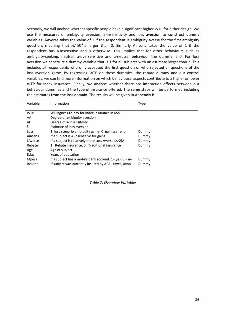
26

Secondly, we will analyse whether specific people have a significant higher WTP for either design. We

use the measures of ambiguity aversion, a-insensitivity and loss aversion to construct dummy

variables. AAverse takes the value of 1 if the respondent is ambiguity averse for the first ambiguity

question, meaning that 𝐴𝐴50+is larger than 0. Similarly Ainsens takes the value of 1 if the

respondent has a-insensitive and 0 otherwise. This implies that for other behaviours such as

ambiguity-seeking, neutral, a-oversensitive and a-neutral behaviour the dummy is 0. For loss

aversion we construct a dummy variable that is 1 for all subjects with an estimate larger than 2. This

includes all respondents who only accepted the first question or who rejected all questions of the

loss aversion game. By regressing WTP on these dummies, the rebate dummy and our control

variables, we can find more information on which behavioural aspects contribute to a higher or lower

WTP for index insurance. Finally, we analyse whether there are interaction effects between our

behaviour dummies and the type of insurance offered. The same steps will be performed including

the estimates from the loss domain. The results will be given in Appendix B.

Variable

Information Type

WTP Willingness-to-pay for index insurance in KSh AA Degree of ambiguity aversion AI λ

Degree of a-insensitivity Estimate of loss aversion

Loss 1=loss scenario ambiguity game, 0=gain scenario Dummy Ainsens If a subject is A-insensitive for gains Dummy LAverse If a subject is relatively more Loss Averse (λ>2)A Dummy Rebate 1= Rebate insurance, 0= Traditional insurance Dummy Age Age of subject Educ Years of education Mpesa If a subject has a mobile bank account. 1= yes, 0 = no Dummy Insured If subject was currently insured by APA. 1=yes, 0=no Dummy

Table 7: Overview Variables

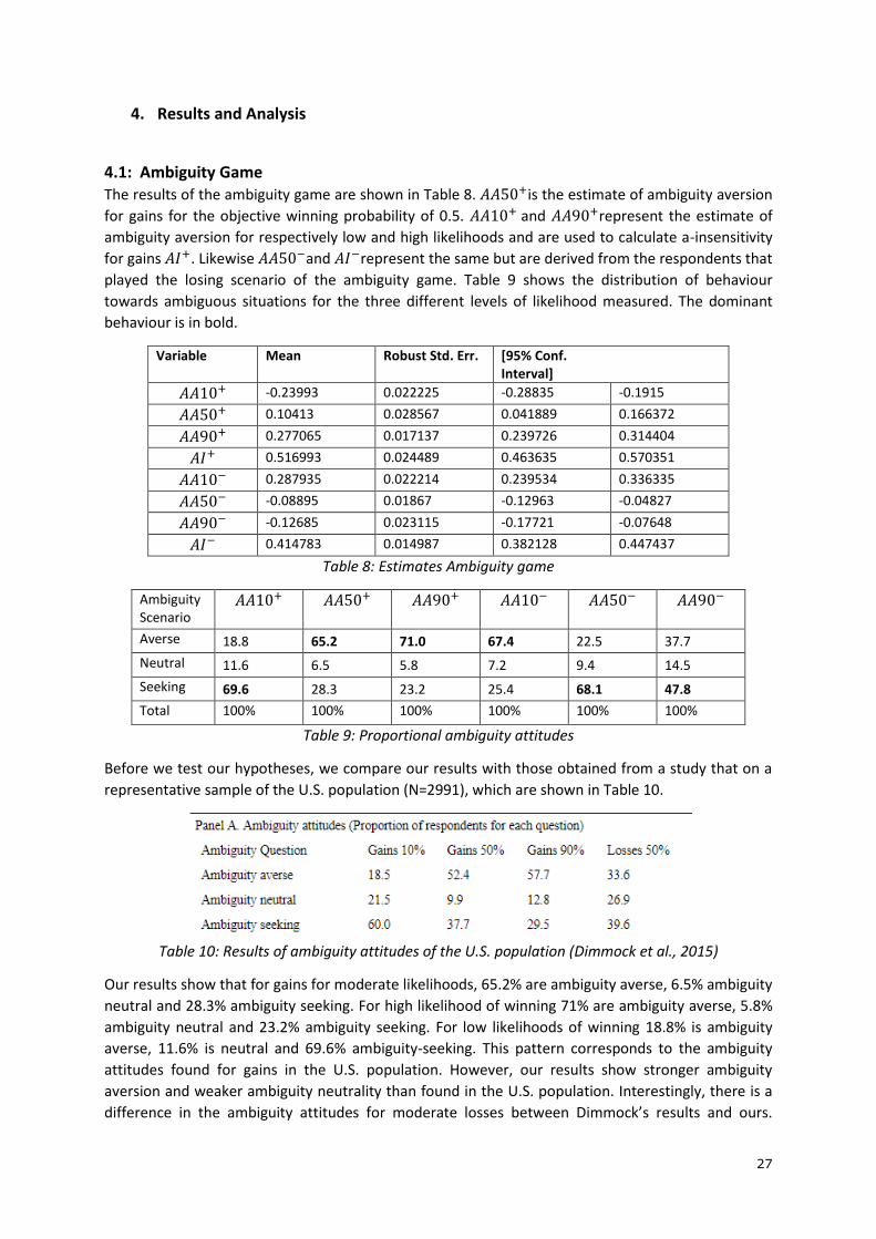
27

4. Results and Analysis

4.1: Ambiguity Game The results of the ambiguity game are shown in Table 8. 𝐴𝐴50+is the estimate of ambiguity aversion

for gains for the objective winning probability of 0.5. 𝐴𝐴10+ and 𝐴𝐴90+represent the estimate of

ambiguity aversion for respectively low and high likelihoods and are used to calculate a-insensitivity

for gains 𝐴𝐼+. Likewise 𝐴𝐴50−and 𝐴𝐼−represent the same but are derived from the respondents that

played the losing scenario of the ambiguity game. Table 9 shows the distribution of behaviour

towards ambiguous situations for the three different levels of likelihood measured. The dominant

behaviour is in bold.

Variable Mean Robust Std. Err. [95% Conf. Interval]

𝐴𝐴10+ -0.23993 0.022225 -0.28835 -0.1915

𝐴𝐴50+ 0.10413 0.028567 0.041889 0.166372

𝐴𝐴90+ 0.277065 0.017137 0.239726 0.314404

𝐴𝐼+ 0.516993 0.024489 0.463635 0.570351

𝐴𝐴10− 0.287935 0.022214 0.239534 0.336335

𝐴𝐴50− -0.08895 0.01867 -0.12963 -0.04827

𝐴𝐴90− -0.12685 0.023115 -0.17721 -0.07648

𝐴𝐼− 0.414783 0.014987 0.382128 0.447437

Table 8: Estimates Ambiguity game

Ambiguity Scenario

𝐴𝐴10+ 𝐴𝐴50+ 𝐴𝐴90+ 𝐴𝐴10− 𝐴𝐴50− 𝐴𝐴90−

Averse 18.8 65.2 71.0 67.4 22.5 37.7

Neutral 11.6 6.5 5.8 7.2 9.4 14.5

Seeking 69.6 28.3 23.2 25.4 68.1 47.8

Total 100% 100% 100% 100% 100% 100%

Table 9: Proportional ambiguity attitudes

Before we test our hypotheses, we compare our results with those obtained from a study that on a

representative sample of the U.S. population (N=2991), which are shown in Table 10.

Table 10: Results of ambiguity attitudes of the U.S. population (Dimmock et al., 2015)

Our results show that for gains for moderate likelihoods, 65.2% are ambiguity averse, 6.5% ambiguity

neutral and 28.3% ambiguity seeking. For high likelihood of winning 71% are ambiguity averse, 5.8%

ambiguity neutral and 23.2% ambiguity seeking. For low likelihoods of winning 18.8% is ambiguity

averse, 11.6% is neutral and 69.6% ambiguity-seeking. This pattern corresponds to the ambiguity

attitudes found for gains in the U.S. population. However, our results show stronger ambiguity

aversion and weaker ambiguity neutrality than found in the U.S. population. Interestingly, there is a

difference in the ambiguity attitudes for moderate losses between Dimmock’s results and ours.

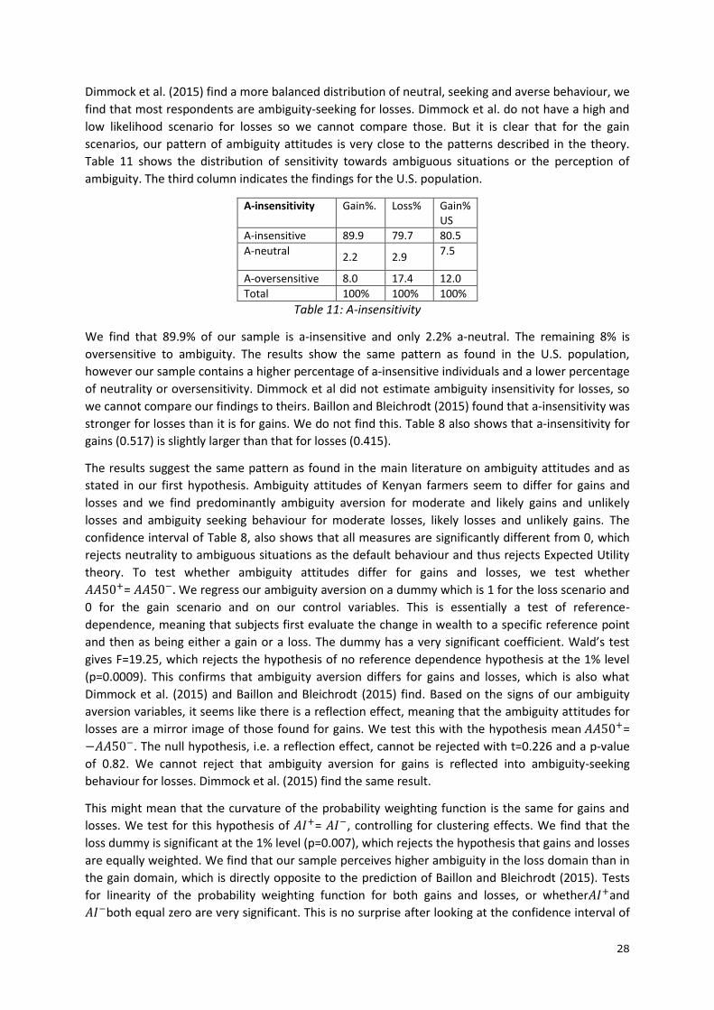
28

Dimmock et al. (2015) find a more balanced distribution of neutral, seeking and averse behaviour, we

find that most respondents are ambiguity-seeking for losses. Dimmock et al. do not have a high and

low likelihood scenario for losses so we cannot compare those. But it is clear that for the gain

scenarios, our pattern of ambiguity attitudes is very close to the patterns described in the theory.

Table 11 shows the distribution of sensitivity towards ambiguous situations or the perception of

ambiguity. The third column indicates the findings for the U.S. population.

A-insensitivity Gain%. Loss% Gain% US

A-insensitive 89.9 79.7 80.5

A-neutral 2.2 2.9

7.5

A-oversensitive 8.0 17.4 12.0

Total 100% 100% 100%

Table 11: A-insensitivity

We find that 89.9% of our sample is a-insensitive and only 2.2% a-neutral. The remaining 8% is

oversensitive to ambiguity. The results show the same pattern as found in the U.S. population,

however our sample contains a higher percentage of a-insensitive individuals and a lower percentage

of neutrality or oversensitivity. Dimmock et al did not estimate ambiguity insensitivity for losses, so

we cannot compare our findings to theirs. Baillon and Bleichrodt (2015) found that a-insensitivity was

stronger for losses than it is for gains. We do not find this. Table 8 also shows that a-insensitivity for

gains (0.517) is slightly larger than that for losses (0.415).

The results suggest the same pattern as found in the main literature on ambiguity attitudes and as

stated in our first hypothesis. Ambiguity attitudes of Kenyan farmers seem to differ for gains and

losses and we find predominantly ambiguity aversion for moderate and likely gains and unlikely

losses and ambiguity seeking behaviour for moderate losses, likely losses and unlikely gains. The

confidence interval of Table 8, also shows that all measures are significantly different from 0, which

rejects neutrality to ambiguous situations as the default behaviour and thus rejects Expected Utility

theory. To test whether ambiguity attitudes differ for gains and losses, we test whether

𝐴𝐴50+= 𝐴𝐴50−. We regress our ambiguity aversion on a dummy which is 1 for the loss scenario and

0 for the gain scenario and on our control variables. This is essentially a test of reference-

dependence, meaning that subjects first evaluate the change in wealth to a specific reference point

and then as being either a gain or a loss. The dummy has a very significant coefficient. Wald’s test

gives F=19.25, which rejects the hypothesis of no reference dependence hypothesis at the 1% level

(p=0.0009). This confirms that ambiguity aversion differs for gains and losses, which is also what

Dimmock et al. (2015) and Baillon and Bleichrodt (2015) find. Based on the signs of our ambiguity

aversion variables, it seems like there is a reflection effect, meaning that the ambiguity attitudes for

losses are a mirror image of those found for gains. We test this with the hypothesis mean 𝐴𝐴50+=

−𝐴𝐴50−. The null hypothesis, i.e. a reflection effect, cannot be rejected with t=0.226 and a p-value

of 0.82. We cannot reject that ambiguity aversion for gains is reflected into ambiguity-seeking

behaviour for losses. Dimmock et al. (2015) find the same result.

This might mean that the curvature of the probability weighting function is the same for gains and

losses. We test for this hypothesis of 𝐴𝐼+= 𝐴𝐼−, controlling for clustering effects. We find that the

loss dummy is significant at the 1% level (p=0.007), which rejects the hypothesis that gains and losses

are equally weighted. We find that our sample perceives higher ambiguity in the loss domain than in

the gain domain, which is directly opposite to the prediction of Baillon and Bleichrodt (2015). Tests

for linearity of the probability weighting function for both gains and losses, or whether𝐴𝐼+and

𝐴𝐼−both equal zero are very significant. This is no surprise after looking at the confidence interval of

29

Table 8. Our test-statistics confirm this and we reject neutrality for the weighting function for gains

with t=76.1 and for losses with t=99.8. Both hypotheses are rejected at the 1% level with p=0.000.

This is in line with the inverse-S function of underweighting high probabilities and overweighting low

probabilities of Prospect Theory. Booij and van de Kuilen (2009) find that most studies report a

measure of probability weighting of around 0.67, which is similar to the transformed estimate for a-

insensitivity of Dimmock et al (2015). They measure a-insensitivity for gains at 0.320. A one-sided t-

test on whether our estimate of a-insensitivity for gains of 0.517 is larger than Dimmock’s estimate of

0.320, yields a highly significant test-statistic with p=0.000. If we transform our measure to the same

scale, i.e. calibrate to 1 for neutrality, we get 0.493 which is thus significantly lower than the average

in the literature on probability weighting. This means that we find more insensitivity to likelihoods,

resulting in a heavier inverse-S shape. We have therefore proven our second hypothesis, we find that

our sample showcases stronger ambiguity generated insensitivity than found in other studies. A-

insensitivity is linked to cognition and can decrease after experience or learning. Our sample has less

experience with probabilities and has less education than the American population, which led us to

this hypothesis.

The results of our first game have confirmed our first and second hypothesis. We find that Kenyan

farmers showcase the same pattern of ambiguity attitudes as found in other studies, on for example

the U.S. population. Kenyan farmers are on average ambiguity averse to moderate and highly likely

gains and also to unlikely losses. They are ambiguity seeking for unlikely gains and moderate and

highly likely losses. Compared with the study conducted on the U.S. population, we find relatively

more a-insensitive individuals and also significantly higher a-insensitivity. Our results are in line with

Prospect Theory, which is flexible in its incorporation of ambiguity attitudes parameters. Key

assumptions of Prospect Theory have been found in our data: reference-dependence, reflection and

probability weighting. Moreover, the data raises more doubts on whether the Multiple Prior models

can explain the full pattern of ambiguity attitudes found in decision making. According to Baillon and

Bleichrodt (2015), the α-MaxMin Model is also a viable option for modelling decision-making under

uncertainty. Besides the implausible assumption of EU under risk, the α-MaxMin Model, cannot

accommodate a-oversensitivity in its parameters (Baillon et al., 2016). It can only explain situations of

a-insensitivity. However 8% of our sample showed oversensitivity to ambiguity generated likelihood

in the gain domain and 17.4% in the loss domain. In contrast, Prospect Theory is able to include a-

oversensitivity and is therefore more appealing for modelling decision making of Kenyan farmers.

4.2: Loss aversion Table 12 depicts the results of the loss aversion game for all three methods of estimation. Our first

estimate of loss aversion assumes equal probability weighting for gains and losses and no diminishing

sensitivity and is obtained by: 𝜆1 = 𝐺/𝐿, where G stands for the fixed gain of 150 KSh and L stands

for the value of the latest choice lottery still accepted by the subject. If all questions are accepted,

L=175, if all questions are rejected L≤50. If only question 1 is accepted and the rest rejected, then

L=50. On average respondents showed loss aversive behaviour. The mean estimate is 2.18 and the

median, which is the most common estimate used in the literature, is 2. It is important to note that

132 observations return to λ=3. Of this segment, 59 subjects rejected all games, resulting in a score

of λ>=3. Similarly, 36 subjects accepted all games and have an estimate of λ <=0.857.

Our second estimation of loss aversion assumes both diminishing sensitivity and probability

weighting, based on the literature review. We take Abdellaoui’s estimate of probability weighting for

gains and losses of ω=0.86 and Booij and vande Kuilen’s estimate of diminishing sensitivity for gains

α=0.859 and losses β=0.826. Our estimate is derived by the following equation:

30

𝜆2 = 0.86 ∗ (𝐺0.859

𝐿0.826 )

Our third estimation of loss aversion has the same assumptions on probability weighting and

diminishing sensitivity, but uses the data derived from the ambiguity game to estimate probability

weighting. We did not derive any measures that allow us to estimate the parameters of diminishing

sensitivity. Using the following equations, we can estimate 𝜆3, where γ is the parameter for

pessimism captured by 𝐴𝐴50+ for gains and 𝐴𝐴50−for losses and 𝛿 is the parameter for likelihood

insensitivity captured by 𝐴𝐼+and 𝐴𝐼−.

𝜔(𝑝) =𝛿𝑝𝛾

𝛿𝑝𝛾 + (1 − 𝑝)𝛾

𝜆3 = 𝜔 ̂ ∗ (𝐺0.859

𝐿0.826 )

To avoid outliers we take the medians of the ambiguity attitudes, which gives us 𝐴𝐼+=0.515,

𝐴𝐼−=0.435, 𝐴𝐴50+=0.135 and 𝐴𝐴50−=-0.12. We will have to transform our measures to make them

in line with the parameters of probability weighting which are calibrated to 1, whereas our measures

are 0 for neutrality. We therefore transform our measures to be 1 for neutrality. Again we take the

medians and get 𝛿+=0.865, 𝛿−=1.12, reflecting pessimism in both domains and 𝛾+=0.485 and

𝛾−=0.565, reflecting insensitivity for extreme likelihoods, stronger for gains than for losses. We take

the mean estimates of elevation and curvature and use those to calculate 𝜔+=0.463 and 𝜔−=0.528.

This yields a probability weighting function of 0.463/0.528=0.877 which lies very close to the average

of 0.86 obtained in other studies. Unsurprisingly, the measures of loss aversion of our second and

third estimation method are very similar.

α=β=1; ω=1 α=0.859; β=0.826; ω=0.86

α=0.859; β=0.826; ω=0.877

λ1 λ2 λ3 Freq. Percent

Accept All ≤0.86 ≤0.89 ≤0.91 28 10.1

Reject #6 1 1.01 1.03 12 4.3

Reject #5 1.2 1.18 1.20 22 8.0

Reject #4 1.5 1.42 1.44 40 14.5

Reject #3 2 1.8 1.83 42 15.2

Reject #2 3 2.51 2.56 73 26.4

Reject all ≥3 ≥2.51 ≥2.56 59 21.4

Total 276 100%

Mean 2.18 1.91 1.94

Median 2 1.8 1.83

Table 12: Three estimates of Loss aversion

Table 12 shows that imposing stricter assumptions on the parameters yields a lower estimate of loss

aversion for 𝜆2 and 𝜆3 However, even if we take strong assumptions on the parameters for

diminishing sensitivity and probabilistic weighting for gains and losses, we get a median between 1.8

and 1.83. All three estimates of loss aversion are significantly larger than 1 with p-values of 0.000,

which confirms that loss aversion plays a role in decision making for our sample and supports the

usage of PT. This confirms our third hypothesis that Kenyan farmers are on average loss averse.

31

This is a plausible result and similar to the estimate found in other studies. Booij and Kuilen (2009)

find 1.58 and 1.87 (2007), whereas Gächter’s (2010) study yields 1.29. It should be noted that the

method of estimation, parametric, non-parametric and assumptions on the estimates of diminishing

sensitivity and probability weighting are important in determining the degree of loss aversion. The

original estimate of Kahneman and Tversky (1992) is 2.25, which is often used as a focal point in

modelling Prospect Theory. It is colloquially cited to state that losses are twice as strongly

experienced as gains. Many recent studies, however, find values lower than 2 raising doubts on the

original estimate. Depending on our parameterisation we get a median between 1.8 and 2. Our

sample consists of subsistence farmers, who are on average poorer than Western counterparts and

therefore the losses used in the experiment might have a greater impact on their wealth relative to

Western respondents. It thus makes sense that our estimate of loss aversion is on the high end of

recent literature. We find that an average farmer in Kenya experiences a loss almost twice as intense

as a gain of the same size, which is in line with Prospect Theory. This has important consequences for

decision making, particularly for financial goods such as insurance products.

4.3: Willingness-to-Pay and Analysis The results of our WTP-game show that the mean WTP for the traditional insurance is 843 KSh with a

standard error of 51 KSh, whereas the rebate type has a mean WTP of 900 KSh and a standard error

of 66. The mean WTP of the rebate insurance is thus slightly higher, but this difference is not

significant, which is also found when regressing WTP on our control variables and our rebate dummy

variable. The coefficient of the rebate dummy has a positive sign but Wald’s test on the coefficient of

the treatment (rebate) dummy gives F=0.19 with a p-value of 0.67, which does not confirm our

hypothesis that WTP for the rebate type is significantly higher. Regressing WTP on either the gain or

loss ambiguity attitudes and the rebate dummy and control variables also finds no significant

difference between insurance type. The only significant effect we find is being currently insured,

which has a significant negative effect on WTP (p=0.043). This could mean that there is an anchoring

effect to the price they are used to pay for the insurance. The signs of the coefficients of the

ambiguity attitudes are as expected with negative signs for the gain attitudes and positive signs for

the loss attitudes. The negative signs imply that ambiguity averse and a-insensitive subjects are

willing to pay less for index insurance because they respectively dislike and overweight (the

probability of) basis risk. These findings provide evidence toward the validity of our third hypothesis,

i.e. ambiguity aversion and a-insensitivity for gains are negatively correlated to WTP for both

insurance designs due to basis risk. However, we only find significant evidence of this relation for a-

insensitivity. Furthermore, we do not find any evidence to claim that this negative relation is less

strong for the rebate type of insurance.

To analyse the relation between our behavioural attitudes and WTP and whether some of these

traits can be linked to preferring one insurance type over the other, we include dummy variables. Of

the respondents that participated in the gain ambiguity scenario, 47.8% falls into the relatively more

loss averse category, 65.2% is ambiguity averse and 89.9% is a-insensitive. We regress WTP on a

dummy variable for ambiguity aversion, loss aversion and a-insensitivity, the rebate dummy and our

control variables. We find that our a-insensitivity dummy is significantly negative (p=0.085). This

means that a-insensitive subjects have a significantly lower WTP for index insurance designs than

subjects who are not a-insensitive. The coefficients for the loss averse and ambiguity averse

dummies are negative but insignificant. Being insured also has a significant negative effect on WTP

(p=0.059). The results can be found in column 1 of Table 13. Column 2, 3 and 4 depict additional

regressions, where in each regression one of the three behavioural dummies is interacted with the

rebate dummy, while controlling for the other dummies as well as for our other control variables. We

32

find that a-insensitivity and being insured remain significantly negative throughout the regressions.

When interacting ambiguity aversion with the rebate dummy, which is shown in column 2, we find

several significant effects. First of all we find that the coefficients of the ambiguity aversion and

rebate dummies are significantly positive, with p=0.043 and p=0.086. This means that for the

traditional insurance type, ambiguity averse individuals have a significantly higher WTP than those

who are not ambiguity averse. Also, non-averse subjects have a significantly higher WTP for the

rebate type. Secondly, the interaction is significantly negative effect (p=0.043). The interpretation is

that the negative effect on WTP of begin ambiguity averse is significantly stronger when the rebate

type of insurance is offered rather than the traditional insurance. Ambiguity averse subjects thus

have a lower WTP for the rebate type insurance over the traditional type, than the non-ambiguity

averse. This goes against our hypothesis and the ideas of Serfilippi et al. (2016) However, considering

the fact that the rebate type of insurance essentially increases the degree of uncertainty, it is not

unimaginable that ambiguity averse individuals dislike this type of insurance policy.

With regards to our fourth and fifth hypothesis, interacting loss aversion with the rebate yields no

significant results. We do find that the coefficients of loss aversion flip from being negative for the

traditional type to positive for the rebate type, but this is not significant. We expected that the loss

averse subjects would have a higher WTP for the rebate insurance due to a framing effect. The stand-

alone investment frame would change due to the removal of certainty of paying the premium

towards a larger frame, where the possible loss would be larger. Loss averse individuals would want

to ensure against this larger possible loss and thus have a higher WTP for the rebate type. If this were

the case, we do not provide evidence to substantiate our fourth and fifth hypothesis. Further

research is warranted to investigate how and if framing effects of index insurance design can alter

the reference point assumed when making insurance purchasing decisions and how this relates to

ambiguity attitudes and loss aversion. Interacting a-insensitivity with the rebate dummy also yields

no significant findings.

At first glance we find no significant difference between the two insurance types. Using dummies for

specific behavioural attitudes suggests that a-insensitive individuals, who take up 90% of the sample,

have a significantly lower WTP for both insurance types than those who are not a-insensitive. This

confirms our hypothesis. Surprisingly, we find that the ambiguity averse individuals have a

significantly lower WTP for the rebate type over the traditional insurance. This rejects our hypothesis

that WTP would be higher for the rebate type. Doing the same regressions with the estimates

obtained from the loss scenarios of the ambiguity games, yields no significant results with respect to

ambiguity attitudes and loss aversion.12 The results can be found in Appendix B.

12 The coefficient for being insured is significantly positive. The coefficient of the constant is

however no longer significantly larger than 0.

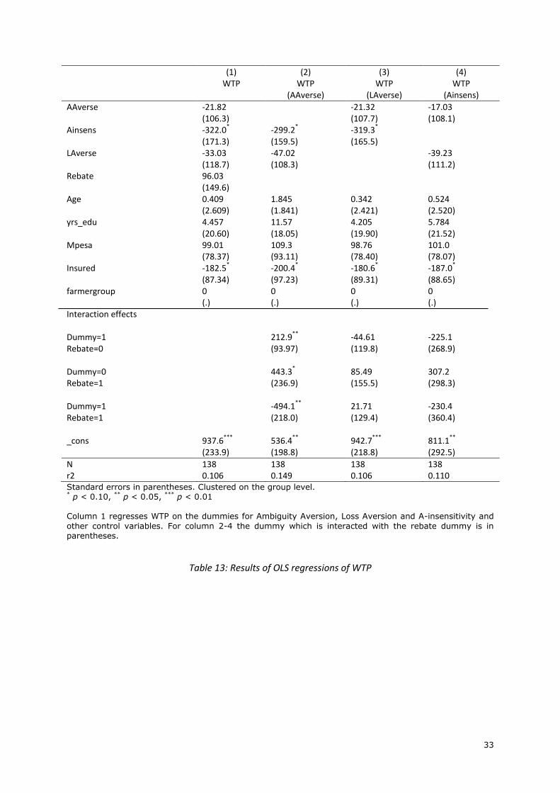
33

(1) (2) (3) (4) WTP WTP

(AAverse) WTP

(LAverse) WTP

(Ainsens)

AAverse -21.82 -21.32 -17.03 (106.3) (107.7) (108.1) Ainsens -322.0

* -299.2

* -319.3

*

(171.3) (159.5) (165.5) LAverse -33.03 -47.02 -39.23 (118.7) (108.3) (111.2) Rebate 96.03 (149.6) Age 0.409 1.845 0.342 0.524 (2.609) (1.841) (2.421) (2.520) yrs_edu 4.457 11.57 4.205 5.784 (20.60) (18.05) (19.90) (21.52) Mpesa 99.01 109.3 98.76 101.0 (78.37) (93.11) (78.40) (78.07) Insured -182.5

* -200.4

* -180.6

* -187.0

*

(87.34) (97.23) (89.31) (88.65) farmergroup 0 0 0 0 (.) (.) (.) (.) Interaction effects

Dummy=1 212.9**

-44.61 -225.1 Rebate=0 (93.97)

(119.8) (268.9)

Dummy=0 443.3* 85.49 307.2

Rebate=1 (236.9)

(155.5) (298.3)

Dummy=1 -494.1**

21.71 -230.4 Rebate=1 (218.0)

(129.4) (360.4)

_cons 937.6***

536.4**

942.7***

811.1**

(233.9) (198.8) (218.8) (292.5)

N 138 138 138 138 r2 0.106 0.149 0.106 0.110 Standard errors in parentheses. Clustered on the group level. * p < 0.10, ** p < 0.05, *** p < 0.01 Column 1 regresses WTP on the dummies for Ambiguity Aversion, Loss Aversion and A-insensitivity and

other control variables. For column 2-4 the dummy which is interacted with the rebate dummy is in parentheses.

Table 13: Results of OLS regressions of WTP

34

5. Discussion There are several limitations to our study. First of all, the selection of the farmer groups for this study

was not completely random. We only included groups and subjects that took part in a previous

household survey in March 2017. Out of 40 farmer groups that participated in this March survey, we

selected 13 groups based on group size and practical reasons. We were in the midst of the rainy

season and some of the farmer groups were located 3 hours away of which more than an hour off a

main road. These places were inaccessible and there was a risk that we would get stuck and not be

able to come back. This meant that in selecting the towns, we had to take into account the

accessibility of the place. This may have led to biases due to excluding farmer groups in this study

that were more remote.

Secondly, by splitting up our sample into 2 groups for the ambiguity game, the sample size was

reduced drastically. For the regressions of WTP on our behaviour dummies we could only include the

people that participated in the ambiguity game for gains (N=138). Of this group, half faced the

traditional insurance and the other the rebate insurance type. This caused a reduction of the power

of our analyses. We used random stratification at the group level, meaning that within every farmer

group, people were randomly assigned which games to play. Even though we restricted the farmers

from sharing information from one to another as much as possible, it is possible that subjects

influenced each other slightly. This could lead to intra-group correlation, especially with respect to

the WTP-game, where they were sitting close together. Even though we did not find any statistically

worrying intra-class correlations, we did decide to cluster our standard errors at the farmer-group

level. If this was redundant, the result would be the same as normal robust standard errors. This

increase in the standard error, however, makes it harder to find any significance. This combination of

reduced sample size and increased standard errors, made it difficult to confirm some of our

hypotheses.

Thirdly, there are reasons to believe that not all farmers fully understood the ambiguity game. We

investigated this with two check questions that measured consistency in the answers given. Out of

287 respondents, only 17 answered both questions correctly, 192 had at least one correct (the

answer indifferent was right nor wrong), 48 had one incorrect and 15 responded both incorrectly.

This raises doubts on the reliability of the data and whether the game might have been too abstract

for good understanding. Removing all observations that had at least one question incorrect was not

possible, as this would drastically reduce our sample size.

Fourthly, the source of uncertainty used is another limitation. Baillon et al. (2016, p 2) reviews that

“several authors warned against the focus on artificial ambiguities, arguing for the importance of

natural events”, among whom Ellsberg himself. Abdellaoui (2011) shows that ambiguity attitudes are

dependent on the source of ambiguity and argues that artificial sources might induce different

responses than those faced in reality. Baillon and Bleichrodt (2015) do not find this difference. Baillon

et al. (2016) find no significant ambiguity aversion on a study on students while using a familiar

source of uncertainty: changes on the stock market. Initially, we designed a game where we would

take a natural source of uncertainty of something related to the weather. Then we came up with a

design of 2 bottles of different shapes filled with maize kernels. They could choose between the

ambiguous option of e.g. bottle 1 weighs more than bottle 2 or a risky option of a winning chance of

50%. Matching probabilities and ambiguity attitudes would be derived from a point of indifference

between the risky and ambiguous option, following the methodology of Baillon et al. (2016). While

piloting we found that this caused great confusion to the farmers, especially when the ambiguous

event with high likelihood occurred. This had two winning statements, for example you win if bottle 2

weighs less than bottle 1 or weighs the same amount. We therefore went back to a simpler artificial

35

source of ambiguity with as much visualisation as possible, as described in this study. Unfortunately,

the consistency questions reveal that understanding of the game was for some subjects difficult.

Similarly, to avoid confusion we decided to exclude upside basis risk from the WTP-game. Upside

basis risk is the possibility of receiving a pay-out of the insurance while also experiencing a good

harvest. If we would have included this, it is probable that ambiguity-seeking or optimistic individuals

would have reacted more positively to this than ambiguity averse individuals. This would be an

interesting topic for additional research.

Furthermore, there might have been quite some anchoring effects for the WTP-game. As explained in

section 3.5, there might have been an anchoring effect from the March household survey WTP-game.

Also 19.9% of our sample was insured at the time of our framed field experiment, which we found to

significantly decrease WTP for both types of insurance, using the gain ambiguity attitudes. This

implies that there was a strong anchoring effect. We tried to reduce both possible anchoring effects

by setting a price range of which the lower boundary was the same as the highest possible price they

could have anchored to (400 KSh) after the March survey. We found no anchoring effects for the

March-session. However, the setting of the price range, might have caused some anchoring by itself.

The results of our WTP-game should therefore not be interpreted as true demand, or actual prices

they will pay for insurance.

Finally, in every game we endowed people with a participation fee. We did not want our participants

to use their own money and possibly losing some of it. This could have led to an endowment effect, if

subjects integrated their endowment and therefore considered it as a gain scenario. Other studies

like Baillon and Bleichrodt (2015) find no significant differences between ambiguity attitudes for

losses measured with real or hypothethical losses. Also, Etchart-Vincent and l’Haridon (2011) find

that hypothethical versus real losses only differ in the gain domain. We therefore do not expect that

our sample exhibited an endowment effect. Moreover, if they would have considered it as an

eventual gain, we would not have found significant differences between the ambiguity attitudes for

gains and losses.

36

6. Conclusion This study confirms that there is much variety in how people respond to ambiguous situations.

Confirming the main literature on ambiguity attitudes, we show that Kenyan subsistence farmers are

on average ambiguity averse to moderate and highly likely gains and also to unlikely losses. They are

ambiguity seeking for unlikely gains and moderate and highly likely losses. Moreover, they are

significantly loss averse. We also confirm that Kenyan farmers are more a-insensitive than found in

Western studies, which means that they are less able to discriminate between different likelihoods

leading to perceiving them as probabilities of fifty-fifty. Our findings are in line with Prospect Theory,

which is flexible in its incorporation of ambiguity attitudes parameters. Key assumptions of Prospect

Theory have been found in our data: reference-dependence, reflection, probability weighting and

loss aversion.

We expected to find that ambiguity aversion and a-insensitivity are negatively correlated to WTP for

both index-insurance types due to basis risk. Our study confirms this relation, with only a-insensitivity

having a significant negative effect on WTP. The widespread a-insensitivity, 90% of our sample falls

into this category, implies that farmers in rural Kenya overweight the probability of not being paid

out while buying insurance and experiencing a bad harvest. This is the probable cause of the

significantly negative effect on WTP observed. Our study finds no significant difference between

willingness-to-pay for the traditional index insurance and the rebate type. Also, we expected to find

that loss aversion would be negatively correlated to the traditional index insurance and positively to

the rebate type due to a framing effect. The coefficient does change from negative for the traditional

type of insurance to positive for the rebate, but this is very insignificant. We do not find enough

evidence to proof that loss aversion significantly affects WTP, or that this has to do with a framing

effect due to removing the certainty effect, inducing farmers to assume a higher reference point

when assessing the rebate insurance. Surprisingly, we find that that the negative effect on WTP of

being ambiguity averse is significantly stronger for the rebate insurance than for the traditional

insurance. This can be explained by the fact that the rebate type essentially increases ambiguity in its

design and is therefore valued less by ambiguity averse people. Unfamiliarity of the new design could

also play a role. Loosely put, pessimistic people dislike an insurance design with more uncertainty

more than an insurance with less uncertainty.

This study contributes to a richer understanding of how farmers’ perceive and respond to index

insurance designs. It shows that farmers’ perception of index insurance designs is rather negative

due to a dislike of ambiguity and overweighting of the likelihood of basis risk. Insurance design

should be better attuned to these dominant ambiguity attitudes. As long as the presence of basis risk

cannot significantly be reduced or as long as farmers in rural Kenya remain strongly a-insensitive,

uptake of index insurance is unlikely to grow. It is important that more research is done on

alternative designs, including as well upside basis risk, that are impacted less negatively by ambiguity

attitudes.

37

7. References

Abdellaoui, M., Baillon, A., Placido, L., & Wakker, P. (2011). The Rich Domain of Uncertainty: Source Functions and Their Experimental Implementation. American Economic Review, 101(2), 695-723. http://dx.doi.org/10.1257/aer.101.2.695

Abdellaoui, M., Bleichrodt, H., L’Haridon, O., & van Dolder, D. (2016). Measuring Loss Aversion under Ambiguity: A Method to Make Prospect Theory Completely Observable. Journal Of Risk And Uncertainty, 52(1), 1-20. http://dx.doi.org/10.1007/s11166-016-9234-y

Africapay.org. (2015). Minimum Wage Rate per Occupation and Area of Kenya - Africapay.org/Kenya. [online] Available at: http://www.africapay.org/kenya/home/salary/minimum-wages

Allais, M. (1953). Le comportement de l’homme rationnel devant le risque: Critique des postulats et axiomes de l’école américaine. Econometrica, (21), 503-546. http://dx.doi.org/10.2307/1907921

Al-Nowaihi, A., & Dhami, S. (2010). The behavioral economics of the demand for insurance. Retrieved from https://www.le.ac.uk/economics/sd106/Insurance.pdf

Andreoni, B. J., & Sprenger, C. (2012). Risk Preferences Are Not Time Preferences, The American Economic Review, 102(7), 3357–3376.

Andreoni, B. J., & Sprenger, C. (2016). American Economic Association Estimating Time Preferences from Convex Budgets Author ( s ): James Andreoni and Charles Sprenger Source : The American Economic Review , Vol . 102 , No . 7 ( DECEMBER 2012 ), pp . 3333-3356 Published by : American Economic A, 102(7), 3333–3356.

Attanasi, G., Gollier, C., Montesano, A., & Pace, N. (2014). Eliciting ambiguity aversion in unknown and in compound lotteries: a smooth ambiguity model experimental study. Theory and Decision, 77(4), 485–530. https://doi.org/10.1007/s11238-013-9406-z

Babcock, B. A. (2015). Using Cumulative Prospect Theory to Explain Anomalous Crop Insurance Coverage Choice. American Journal of Agricultural Economics, 97(5), 1371–1384. https://doi.org/10.1093/ajae/aav032

Baillon, A. & Bleichrodt, H. (2015). Testing Ambiguity Models through the Measurement of Probabilities for Gains and Losses. American Economic Journal: Microeconomics, 7(2), 77-100. http://dx.doi.org/10.1257/mic.20130196

Baillon, A., Bleichrodt, H., Keskin, U., Haridon, O., & Li, C. (2017). The Effect of Learning on Ambiguity Attitudes. Management Science, June.

Baillon, A., Huang, Z., Selim, A., & Wakker, P. P. (2015). Measuring Ambiguity Attitudes for All ( Natural ) Events, Unpublished manuscript. (September).

Baillon, A., Liu, N., & van Dolder, D. (2017). Comparing uncertainty aversion towards different sources. Theory and Decision, 83(1). https://doi.org/10.1007/s11238-016-9584-6

Barberis, N. C. (2013). Thirty Years of Prospect Theory in Economics: A Review and Assessment. Journal of Economic Perspectives, 27(1), 173–196. https://doi.org/10.2307/41825467

38

Booij, A. S., van Praag, M. S., van de Kuilen. (2010). A parametric analysis of prospect theory’s functionals for the general population. Theory and Decision, 68(1-2), 115-148.

Brown, J. R., Kling, J. R., Mullainathan, S., & Wrobel, M. V. (2008). Why Don’t People Choose Annuities? A Framing Explanation of the under-Annuitization Puzzle. American Economic Review, 98(2), 304–309.

Cai, J. (2016). The impact of insurance provision on household production and financial decisions. American Economic Journal: Economic Policy, 8(2), 44–88. https://doi.org/10.1257/pol.20130371

Carter, M., Elabed, G., & Serfilippi, E. (2015). Behavioral economic insights on index insurance design. Agricultural Finance Review Agricultural Finance Review Agricultural Finance Review, 75(1), 8–18. https://doi.org/10.1108/

Clarke, D. J. (2016) A Theory of Rational Demand for Index Insurance. American Economic Journal: Microeconomics 2016, 8(1): 283–306. http://dx.doi.org/10.1257/mic.20140103

Cole, B. S., Giné, X., Tobacman, J., Topalova, P., Townsend, R., & Vickery, J. (2013). Barriers to Household Risk Management: Evidence from Indi. American Economic Journal: Applied Economics, 5(1), 104–135. https://doi.org/10.1257/app.5.1.104

de Nicola, F. (2015). The impact of weather insurance on consumption, investment, and welfare. Quantitative Economics, 6(3), 637–661. https://doi.org/10.3982/QE300

Dimmock, S. G., Kouwenberg, R., & Wakker, P. P. (2016a). Ambiguity attitudes in a large representative sample. Management Science, 62(5), 1363–1380. https://doi.org/10.1287/mnsc.2015.2198

Dimmock, S. G., Kouwenberg, R., Mitchell, O. S., & Peijnenburg, K. (2015). Estimating ambiguity preferences and perceptions in multiple prior models: Evidence from the field. Journal of Risk and Uncertainty, 51(3), 219–244. https://doi.org/10.1007/s11166-015-9227-2

Dimmock, S. G., Kouwenberg, R., Mitchell, O. S., & Peijnenburg, K. (2016b). Ambiguity aversion and household portfolio choice puzzles: Empirical evidence. Journal of Financial Economics, 119(3), 559–577. https://doi.org/10.1016/j.jfineco.2016.01.003

Elabed, G., & Carter, M. R. (2015). Compound-risk aversion, ambiguity and the willingness to pay for microinsurance. Journal of Economic Behavior and Organization, 118, 150–166. https://doi.org/10.1016/j.jebo.2015.03.002

Ellsberg, D. (1961). Risk, Ambiguity, and the Savage Axioms. Quarterly Journal of Economics, 75(4), 643–669.

Etchart-Vincent, N. & l’Haridon, O. (2011). Monetary incentives in the loss domain and behavior toward risk: An experimental comparison of three reward schemes including real losses. Journal of Risk and Uncertainty, 42(1), 61-83.

Falco, C., Kong, D., Rotondi, V., & Spelta, V. (2016). Investment , Insurance and Weather Shocks: Evidence from a Lab Experiment in Cambodia. 10(July), 1–38.

39

Fehr-Duda, H., & Epper, T. (2012). Probability and Risk: Foundations and Economic Implications of Probability-Dependent Risk Preferences. Annual Review of Economics, 4(1), 567–593. https://doi.org/10.1146/annurev-economics-080511-110950

Fehr, E. and Goette, L. (2007). Do Workers Work More if Wages Are High? Evidence from a Randomized Field Experiment. The American Economic Review, 97(1), pp.298-317.

Gächter, S., Johnson, E. J., & Herrmann, A. (2010). Individual-level loss aversion in riskless and risky choices. CeDEx Discussion Paper Series, (2010–20), 26. https://doi.org/10.1007/s10273-011-1262-2

Giné, X., Townsend, R., & Vickery, J. (2008). Patterns of rainfall insurance participation in rural India. World Bank Economic Review, 22(3), 539–566. https://doi.org/10.1093/wber/lhn015

Hakizimana, C., Goldsmith, P., Nunow, A., Roba, A. and Biashara, J. (2017). Land and agricultural commercialisation in Meru County, Kenya: evidence from three models. The Journal of Peasant Studies, 44(3), pp.555-573.

Halevy, Y. (2007). Ellsberg Revisited: An Experimental Study. Econometrica, 75(2), 503-536. http://dx.doi.org/10.1111/j.1468-0262.2006.00755.x

Hill, R. V., & Viceisza, A. (2012). A field experiment on the impact of weather shocks and insurance on risky investment. Experimental Economics, 15(2), 341–371. https://doi.org/10.1007/s10683-011-9303-7

Janzen, S. A., & Carter, M. R. (2013). The Impact of Microinsurance on Consumption Smoothing and Asset Protection: Evidence from a Drought in Kenya. NBER Working Paper No. 19702.

Kahneman, D. & Tversky, A. (1979). Prospect Theory : An Analysis of Decision under Risk Econometrica, 47(2), 263–292.

Knight, F. H. (1921). Risk, Uncertainty and Profit. Houghton Mifflin.

Köbberling, V., & Wakker, P. P. (2005). An index of loss aversion. Journal of Economic Theory, 122(1), 119–131. https://doi.org/10.1016/j.jet.2004.03.009

Köszegi, B. & Rabin, M. (2007). Reference-Dependent Risk Attitudes. The American Economic Review, 97(4), 1047-1073.

Li, C. (2016). Are the poor worse at dealing with ambiguity ? Are the poor worse at dealing with ambiguity ? Unpublished manuscript. https://doi.org/10.13140/RG.2.1.3556.8406/2

Quiggin, J. (1982). A Theory of Anticipated Utility. Journal of Economic Behaviour and Organization, 3, 323–343.

Rabin, M. 2000. Risk aversion and expected-utility theory: A calibration theorem. Econometrica, 68(5), 1281-1293.

Ramsey, F. P. (1931). Truth and Probability. The Foundations of Mathematics and Other Logical Essays, Ch. VII(1926), 156–198. https://doi.org/10.1007/978-3-319-20451-2_3

40

Savage, L. J. (1954). The Foundations of Statistics. New York: Wiley.

Serfilippi, E., Carter, M., & Guirkinger, C. (2016). Insurance Constracts when Farmers “Greatly Values Certainty:” Results from Field Experiments in Burkina Faso, 1–19. Unpublished manuscript. Retrieved from https://arefiles.ucdavis.edu/uploads/filer_public/99/92/9992afde-bb46-4acb-9aa4-3a5e048a797a/greatly_value_certainty_v1.pdf

Sydnor, J. (2010). (Over)insuring modest risks. American Economic Journal: Applied Economics, 2(4), 177–199. https://doi.org/10.1257/app.2.4.177

The Star, Kenya. (2017). Uhuru announces 18% increase to minimum wage. [online] Available at: http://www.the-star.co.ke/news/2017/05/01/uhuru-announces-18-increase-to-minimum-wage_c1552901 [Accessed 22 Jun. 2017].

Tversky, A., & Kahneman, D. (1992). Advances in Prospect-Theory - Cumulative Representation of Uncertainty. Journal of Risk and Uncertainty, 5(4), 297–323. https://doi.org/Doi 10.1007/Bf00122574

Unicef. (2017). Nutrition crisis deepening across Kenya. [online] Available at: https://www.unicef.org/media/media_100836.html [Accessed 26 Jul. 2017].

Wakker, P. P. (2010). Prospect Theory For Risk and Ambiguity. Cambridge University Press.

Wakker, P., & Tversky, A. (1993). An axiomatization of cumulative prospect theory. Journal of Risk and Uncertainty, 7(2), 147–175. https://doi.org/10.1007/BF01065812

Wakker, P. P. "uncertainty." The New Palgrave Dictionary of Economics. Second Edition. Eds. Steven N. Durlauf and Lawrence E. Blume. Palgrave Macmillan, 2008. The New Palgrave Dictionary of Economics Online. Palgrave Macmillan.

Werner, J. "risk aversion." The New Palgrave Dictionary of Economics. Second Edition. Eds. Steven N. Durlauf and Lawrence E. Blume. Palgrave Macmillan, 2008. The New Palgrave Dictionary of Economics Online. Palgrave Macmillan.

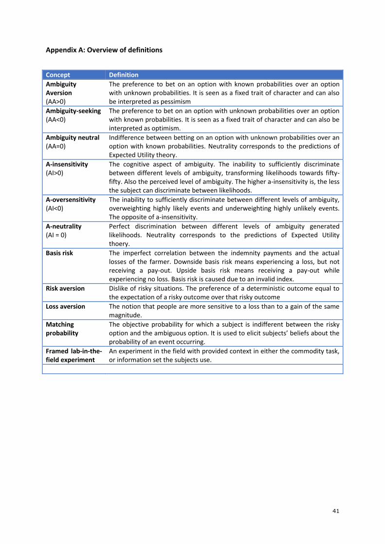
41

Appendix A: Overview of definitions

Concept Definition

Ambiguity Aversion (AA>0)

The preference to bet on an option with known probabilities over an option with unknown probabilities. It is seen as a fixed trait of character and can also be interpreted as pessimism

Ambiguity-seeking (AA<0)

The preference to bet on an option with unknown probabilities over an option with known probabilities. It is seen as a fixed trait of character and can also be interpreted as optimism.

Ambiguity neutral (AA=0)

Indifference between betting on an option with unknown probabilities over an option with known probabilities. Neutrality corresponds to the predictions of Expected Utility theory.

A-insensitivity (AI>0)

The cognitive aspect of ambiguity. The inability to sufficiently discriminate between different levels of ambiguity, transforming likelihoods towards fifty-fifty. Also the perceived level of ambiguity. The higher a-insensitivity is, the less the subject can discriminate between likelihoods.

A-oversensitivity (AI<0)

The inability to sufficiently discriminate between different levels of ambiguity, overweighting highly likely events and underweighting highly unlikely events. The opposite of a-insensitivity.

A-neutrality (AI = 0)

Perfect discrimination between different levels of ambiguity generated likelihoods. Neutrality corresponds to the predictions of Expected Utility thoery.

Basis risk The imperfect correlation between the indemnity payments and the actual losses of the farmer. Downside basis risk means experiencing a loss, but not receiving a pay-out. Upside basis risk means receiving a pay-out while experiencing no loss. Basis risk is caused due to an invalid index.

Risk aversion Dislike of risky situations. The preference of a deterministic outcome equal to the expectation of a risky outcome over that risky outcome

Loss aversion The notion that people are more sensitive to a loss than to a gain of the same magnitude.

Matching probability

The objective probability for which a subject is indifferent between the risky option and the ambiguous option. It is used to elicit subjects’ beliefs about the probability of an event occurring.

Framed lab-in-the-field experiment

An experiment in the field with provided context in either the commodity task, or information set the subjects use.

42

Appendix B

(1) (2) (3) (4) WTP WTP

(AAverse_L) WTP

(LAverse_L) WTP

(Ainsens_L)

AAverse_L 128.7 139.2 91.05 (162.6) (170.0) (155.3)

Ainsens_L -15.47 -0.527 -2.047 (182.8) (198.3) (191.5)

LAverse -37.25 -40.69 -40.20 (126.6) (123.6) (126.3)

Rebate 53.84 (164.3)

Age 9.728 9.944 9.947 10.96 (6.417) (6.444) (6.378) (6.645)

yrs_edu 14.63 15.66 12.91 13.75 (22.86) (23.45) (22.10) (23.49)

Mpesa 188.3 180.8 192.4 177.8 (124.2) (132.0) (121.3) (138.4)

Insured 634.6** 642.0** 651.5** 671.3** (279.0) (269.1) (287.5) (266.1)

farmergroup 0 0 0 0

(.) (.) (.) (.)

Interaction effects

Dummy=1 Rebate=0

208.0 (138.4)

-174.6 (211.5)

-358.0 (363.4)

Dummy=0 87.51 -65.99 -406.5 Rebate=1 (196.9)

(186.5) (330.5)

Dummy=1 Rebate=1

-141.2 (348.5)

262.7 (278.7)

564.7 (344.3)

_cons 20.24 -27.19 56.70 297.2 (503.8) (529.9) (504.1) (471.5)

N 138 138 138 138 r2 0.184 0.185 0.191 0.203

Standard errors in parentheses. Clustered on the group level. * p < 0.10, ** p < 0.05, *** p < 0.01 Column 1 regresses WTP on the dummies for Ambiguity Aversion for losses, Loss Aversion and A-

insensitivity for losses and other control variables. For column 2-4 the dummy which is interacted with the rebate dummy is in parentheses.