_________________________________________________________________________________________________________

Electrical Engineering Department Los Angeles, California 90095-1594

UNIVERSITY OF CALIFORNIA • LOS ANGELES

Low Temperature Plasma Technology Laboratory

LANGMUIR PROBE MEASUREMENTS IN THE

INTENSE RF FIELD OF A HELICON DISCHARGE

Francis F. Chen

LTP-1205 May, 2012

Langmuir probe measurements in the intense RF field of a helicon discharge Francis F. Chen

Electrical Engineering Department, University of California, Los Angeles, CA 90095-1994

ABSTRACT

Helicon discharges have been extensively studied for over 25 years both because of their intriguing physics and because of their utility in producing high plasma densities for industrial applications. Almost all measurements so far have been made away from the antenna region in the plasma ejected into a chamber where there may be a strong magnetic field (B-field) but where the radiofrequency (RF) field is much weaker than under the antenna. Inside the source region, the RF field distorts the current-voltage (I – V) characteristic of the probe unless it is specially designed with strong RF compensation. For this purpose, a thin probe was designed and used to show the effect of inadequate compensation on electron temperature (Te) measurements. The subtraction of ion current from the I – V curve is essential; and, surprisingly, Langmuir’s Orbital Motion Limited (OML) theory for ion current can be used well beyond its intended regime.

I. Introduction

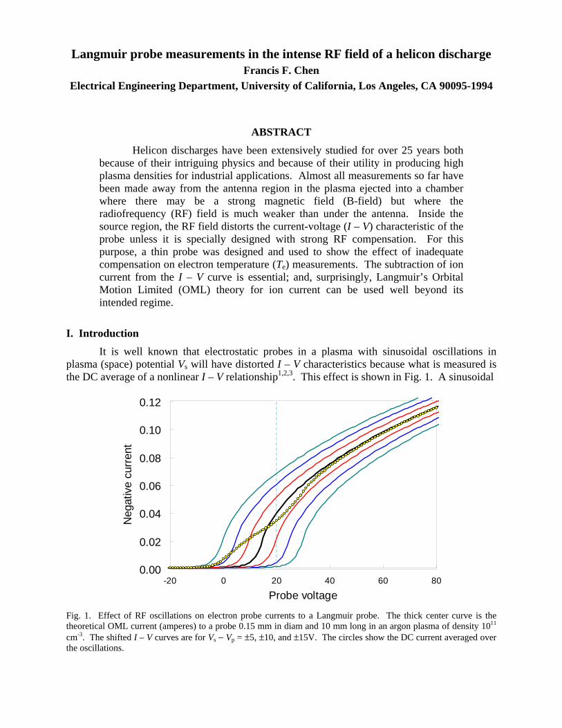
It is well known that electrostatic probes in a plasma with sinusoidal oscillations in plasma (space) potential Vs will have distorted I – V characteristics because what is measured is the DC average of a nonlinear I – V relationship1,2,3. This effect is shown in Fig. 1. A sinusoidal

0.00

0.02

0.04

0.06

0.08

0.10

0.12

-20 0 20 40 60 80

Probe voltage

Neg

ativ

e cu

rren

t

Fig. 1. Effect of RF oscillations on electron probe currents to a Langmuir probe. The thick center curve is the theoretical OML current (amperes) to a probe 0.15 mm in diam and 10 mm long in an argon plasma of density 1011 cm-3. The shifted I – V curves are for Vs − Vp = ±5, ±10, and ±15V. The circles show the DC current averaged over the oscillations.

2oscillation of peak amplitude 15V in plasma potential Vs is assumed. The thick curve at the center is an ideal OML curve, and the side curves show the shifted I – V curves as seen by an uncompensated probe at various phases of the RF. Since the curves are nonlinear, the current averaged over the oscillations will differ from the correct value. For instance, the dashed line shows the current at at probe voltage Vp = 20V . The average over the shifted currents at that voltage would be lower than the unshifted current. What’s worse, the shift stays longer at the extremes of the shift (±15V here) than at other phases as the voltage turns around. The yellow circles (color online) show the DC average current computed taking this effect into account. The result is that the slope of the I – V curve is decreased, leading to a spuriously high apparent KTe. It is seen that the error becomes smaller as the probe approaches electron saturation, where the nonlinearity is less strong.

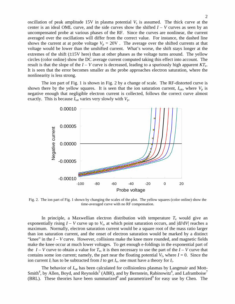
The ion part of Fig. 1 is shown in Fig. 2 by a change of scale. The RF-distorted curve is shown there by the yellow squares. It is seen that the ion saturation current, Isat, where Vp is negative enough that negligible electron current is collected, follows the correct curve almost exactly. This is because Isat varies very slowly with Vp.

-0.00010

-0.00005

0.00000

0.00005

0.00010

-100 -80 -60 -40 -20 0 20

Probe voltage

Neg

ativ

e cu

rren

t

Fig. 2. The ion part of Fig. 1 shown by changing the scales of the plot. The yellow squares (color online) show the

time-averaged curve with no RF compensation.

In principle, a Maxwellian electron distribution with temperature Te would give an exponentially rising I – V curve up to Vs, at which point saturation occurs, and |dI/dV| reaches a maximum. Normally, electron saturation current would be a square root of the mass ratio larger than ion saturation current, and the onset of electron saturation would be marked by a distinct “knee” in the I – V curve. However, collisions make the knee more rounded, and magnetic fields make the knee occur at much lower voltages. To get enough e-foldings in the exponential part of the I – V curve to obtain a value for Te, it is then necessary to use the part of the I – V curve that contains some ion current; namely, the part near the floating potential Vf, where I = 0. Since the ion current Ii has to be subtracted from I to get Ie, one must have a theory for Ii.

The behavior of Isat has been calculated for collisionless plasmas by Langmuir and Mott-Smith4, by Allen, Boyd, and Reynolds5 (ABR), and by Bernstein, Rabinowitz6, and Laframboise7 (BRL). These theories have been summarized8 and parametrized9 for easy use by Chen. The

3BRL and ABR theories have been found to be inaccurate for partially ionized industrial plasmas10, while the Langmuir OML theory appears to be useful well beyond its intended range of applicability11. It is Langmuir’s simple formula for Ii , Eq. (1), that fits experiments well, not his more complete error-function formula, which was used to compute Ie in Fig. 1.

21/2

2,p

i p i p

eVI A ne I V

Mπ

= ∝

. (1)

Here Ap is the probe surface area, n the plasma density, e the unit charge, and M the ion mass. This formula does not depend on KTe, so n can be determined by fitting a straight line to the slope of an I2 – V plot. Once n is known, and if the electrons are Maxwellian, KTe and Vs can be determined from Eq. (2). Here vthe is the electron random thermal velocity. On a plot of ln(Ie) vs. Vp, a straight-line fit’s slope will give KTe, and the line’s horizontal position will yield Vs if n is known. This procedure will be clear when the data are presented.

( )/p s eV V KT

e theI nev e−= . (2)

Some commercial probe systems use Eq. (1) to analyze ion current. For instance, this is done in Hiden Analytical’s ESPsoft® software12, and in the SLP2000 system of Plasmart in Korea (no longer available). Other systems treat ion current differently. The Impedans13 ALP system uses the BRL theory with a correction for collisions. The Korean Wise Probe14 of Chin Wook Chung applies an AC signal to a floating probe and deduces plasma parameters from the harmonics without a direct measurement of Isat. We have chosen to use the OML theory not only because of its simplicity be also because it has been calibrated against microwave interferometry, with result that it is accurate in the 10 mTorr range of pressures and is in error by at most a factor of 2 at 1 mTorr. The use of Eq. (1) and Eq. (2), in that order, yields n and KTe without iteration between them. Some systems require finding Vs from the knee in the I – V curve, but this method fails in the presence of magnetic fields and collisions.

II. Apparatus

A) Helicon discharge. The helicon discharge is shown in Fig. 3. The DC magnetic field is provided by an annular permanent magnet placed in an optimized height above the discharge tube. The use of the remote, reverse field of such a magnet has been described previously15,16,17. The quartz discharge tube has an inner diameter of 5.2 cm and a height of 5.8 cm. The entire superstructure was built only to accommodate the vertical probe; it is not necessary for the discharge. The loop antenna is placed at the bottom to eject the most plasma down into a large chamber. RF frequencies of 27.12 and 13.56 MHz have been used. The magnet height is adjusted to give the B-field for highest downstream density. At 27.12 MHz, this field varies from 80G at the top to 39G at the bottom, with an average of 60G. The chamber above the discharge was made for the vertical probe that probes the discharge interior. It was not possible to make a port for a radial probe without destroying the azimuthal symmetry of this small tube. The top of the discharge is normally a solid, grounded aluminum plate placed so that the helicon wave reflected from it interferes constructively with the downward wave (the Low Field Peak effect18). To insert the probe, the top plate is replaced with one that has a 1/8-inch (3.2mm) diam hole through which two alumina probe shafts are inserted, one for the probe, and the other for the compensation electrode (CE). Other holes, arbitrarily placed, are for pumping the probe extension. Normal operation is at 400W of RF at 27.12 MHz and 15 mTorr of argon, but power

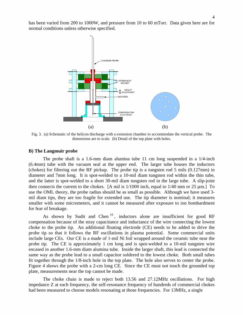
4has been varied from 200 to 1000W, and pressure from 10 to 60 mTorr. Data given here are for normal conditions unless otherwise specified.

(a) (b)

Fig. 3. (a) Schematic of the helicon discharge with a extension chamber to accommodate the vertical probe. The dimensions are to scale. (b) Detail of the top plate with holes.

B) The Langmuir probe

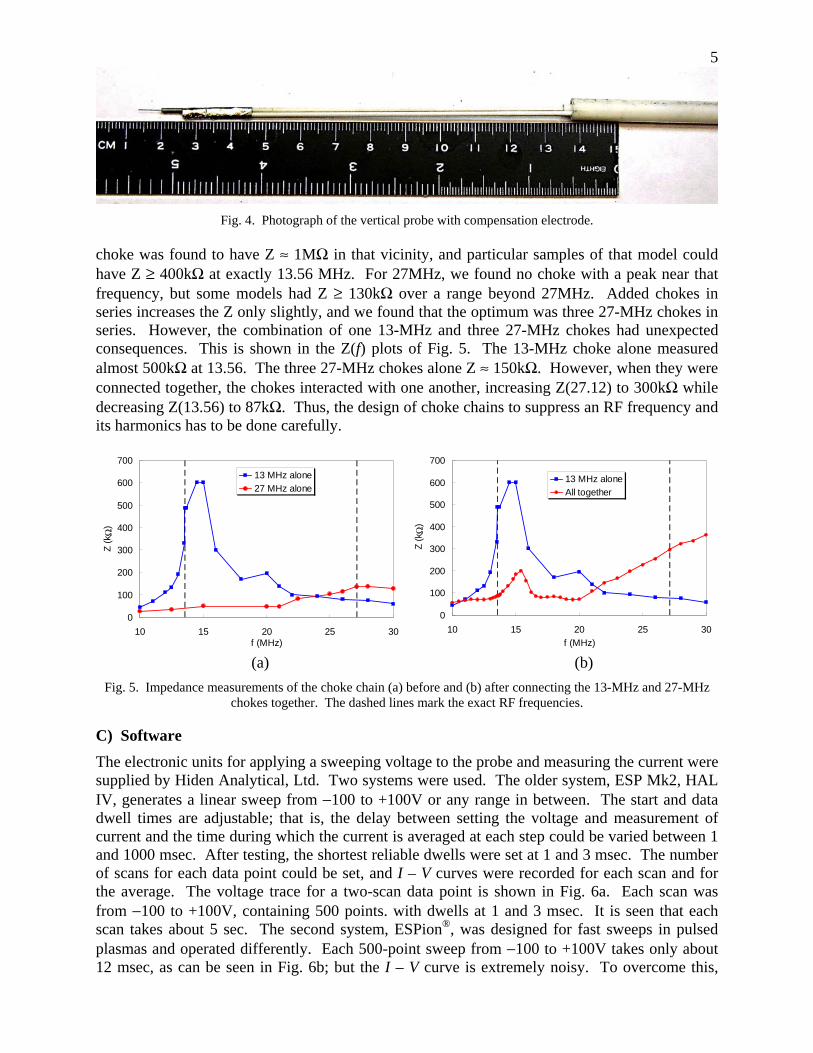
The probe shaft is a 1.6-mm diam alumina tube 11 cm long suspended in a 1/4-inch (6.4mm) tube with the vacuum seal at the upper end. The larger tube houses the inductors (chokes) for filtering out the RF pickup. The probe tip is a tungsten rod 5 mils (0.127mm) in diameter and 7mm long. It is spot-welded to a 10-mil diam tungsten rod within the thin tube, and the latter is spot-welded to a short 30-mil diam tungsten rod in the large tube. A slip-joint then connects the current to the chokes. [A mil is 1/1000 inch, equal to 1/40 mm or 25 μm.] To use the OML theory, the probe radius should be as small as possible. Although we have used 3-mil diam tips, they are too fragile for extended use. The tip diameter is nominal; it measures smaller with some micrometers, and it cannot be measured after exposure to ion bombardment for fear of breakage.

As shown by Sudit and Chen 19 , inductors alone are insufficient for good RF compensation because of the stray capacitance and inductance of the wire connecting the lowest choke to the probe tip. An additional floating electrode (CE) needs to be added to drive the probe tip so that it follows the RF oscillations in plasma potential. Some commercial units include large CEs. Our CE is a made of 1-mil Ni foil wrapped around the ceramic tube near the probe tip. The CE is approximately 1 cm long and is spot-welded to a 10-mil tungsten wire encased in another 1.6-mm diam alumina tube. Inside the larger shaft, this lead is connected the same way as the probe lead to a small capacitor soldered to the lowest choke. Both small tubes fit together through the 1/8-inch hole in the top plate. The hole also serves to center the probe. Figure 4 shows the probe with a 2-cm long CE. Since the CE must not touch the grounded top plate, measurements near the top cannot be made.

The choke chain is made to reject both 13.56 and 27.12MHz oscillations. For high impedance Z at each frequency, the self-resonance frequency of hundreds of commercial chokes had been measured to choose models resonating at those frequencies. For 13MHz, a single

5

Fig. 4. Photograph of the vertical probe with compensation electrode.

choke was found to have Z ≈ 1MΩ in that vicinity, and particular samples of that model could have Z ≥ 400kΩ at exactly 13.56 MHz. For 27MHz, we found no choke with a peak near that frequency, but some models had Z ≥ 130kΩ over a range beyond 27MHz. Added chokes in series increases the Z only slightly, and we found that the optimum was three 27-MHz chokes in series. However, the combination of one 13-MHz and three 27-MHz chokes had unexpected consequences. This is shown in the Z(f) plots of Fig. 5. The 13-MHz choke alone measured almost 500kΩ at 13.56. The three 27-MHz chokes alone Z ≈ 150kΩ. However, when they were connected together, the chokes interacted with one another, increasing Z(27.12) to 300kΩ while decreasing Z(13.56) to 87kΩ. Thus, the design of choke chains to suppress an RF frequency and its harmonics has to be done carefully.

0

100

200

300

400

500

600

700

10 15 20 25 30f (MHz)

Z (

k Ω)

13 MHz alone

27 MHz alone

0

100

200

300

400

500

600

700

10 15 20 25 30

f (MHz)

Z (

k Ω)

13 MHz alone

All together

(a) (b)

Fig. 5. Impedance measurements of the choke chain (a) before and (b) after connecting the 13-MHz and 27-MHz chokes together. The dashed lines mark the exact RF frequencies.

C) Software

The electronic units for applying a sweeping voltage to the probe and measuring the current were supplied by Hiden Analytical, Ltd. Two systems were used. The older system, ESP Mk2, HAL IV, generates a linear sweep from −100 to +100V or any range in between. The start and data dwell times are adjustable; that is, the delay between setting the voltage and measurement of current and the time during which the current is averaged at each step could be varied between 1 and 1000 msec. After testing, the shortest reliable dwells were set at 1 and 3 msec. The number of scans for each data point could be set, and I – V curves were recorded for each scan and for the average. The voltage trace for a two-scan data point is shown in Fig. 6a. Each scan was from −100 to +100V, containing 500 points. with dwells at 1 and 3 msec. It is seen that each scan takes about 5 sec. The second system, ESPion®, was designed for fast sweeps in pulsed plasmas and operated differently. Each 500-point sweep from −100 to +100V takes only about 12 msec, as can be seen in Fig. 6b; but the I – V curve is extremely noisy. To overcome this,

6multiple scans can be taken and averaged by setting the quantity Scan Average (SA). Usable I – V curves could be obtained with SA = 4, but SA = 10−25 gave better curves. To obtain curves as smooth as with the ESP Mk2 required SA = 100. The speed of the ESPion system was needed in the very dense DC plasmas in this work in order to protect the probe. We also needed its maximum current of 1000 mA instead of 100 mA at our densities.

(a) (b)

Fig. 6. Voltage sweeps in the Hiden (a) ESP Mk2 and (b) ESPion probe systems. The vertical scale in both is 50V/div, and the horizontal scales are (a) 5sec/div and (b) 25msec/div.

In both systems the current measuring circuitry was on a floating circuit board which followed the probe voltage. Both systems had adjustments for the number of points in each scan. A probe cleaning voltage up to ±100V of adjustable duration could be applied before each scan in ESP Mk2 and before each bunch of scans in ESPion. However, since spurious voltages at high densities could harm the probe by ion sputtering or heating to electron emission, we cleaned the probe only once after each vacuum pumpdown.

III. Experiment

A. Effect of compensation electrode. Figure 7 shows the ion (I2 – V) and electron (lnIe−V) plots taken with a probe without a compensation electrode (chokes only). The ion plot (Fig. 7a) is almost exactly linear and is typical of all our data. The linearity is a characteristic of orbiting, but it also occurs incidentally in the ABR theory20. However, the ABR theory, which neglects orbiting, gives a spuriously low density10. The density n11 in units of 1011 cm-3 (1017 m-

3) is obtained from Eq. (1) without knowledge of Te. The electron plots in Fig. 7(b-d) were obtained by subtracting the straight-line fit to the ion curve from the total current. We see that there are three regions showing three temperatures, as explained in Figs. (1) and (2). In Fig. 7b, a fit to the slope at high Vp gives KTe = 4.65 eV, which is somewhat higher than the true temperature. In Fig. 7c, a fit to the middle region, which is greatly affected by the RF, yields the spuriously high temperature of 8.22 eV. Such temperatures are often quoted as the true temperature when there is inadequate RF compensation. In Fig. 7d, at fit to the left-most region gives the true temperature of 2.97 eV, since, as shown in Fig. 2, RF has little effect on Ii. Figure 7e shows a typical misinterpretation of Te from a probe with too small a CE, and Fig. 7f shows the correct determination of Te in the same plasma with a large enough CE. A large CE does not affect the spatial resolution of the probe tip, but it may affect the discharge if it is not small compared with the discharge volume.

B. Importance of ion subtraction. In the Ie plots, the solid red curve is the probe current before ion current is subtracted. The true Te is best found from the region where the I – V curve is least affected by RF; namely, the region on the negative side of floating potential Vf.

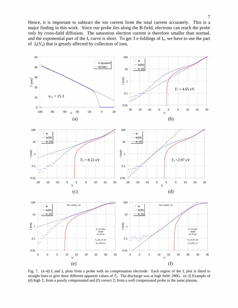
7Hence, it is important to subtract the ion current from the total current accurately. This is a major finding in this work. Since our probe lies along the B-field, electrons can reach the probe only by cross-field diffusion. The saturation electron current is therefore smaller than normal, and the exponential part of the Ie curve is short. To get 3 e-foldings of Ie, we have to use the part of Ie(Vp) that is greatly affected by collection of ions.

(a) (b)

(c) (d)

(e) (f)

Fig. 7. (a−d) Ii and Ie plots from a probe with no compensation electrode. Each region of the Ie plot is fitted to straight lines to give three different apparent values of Te. The discharge was at high field: 280G. (e−f) Example of (d) high Te from a poorly compensated and (f) correct Te from a well compensated probe in the same plasma..

0.01

0.1

1

10

100

-5 0 5 10 15 20 25 30 35V

I (m

A)

Ie

Ie(fit)

Ie (0)

File 110531_15

27.12 MHz400W

15 mTorr

Te=3.57 eV

Vs=33.1 V

0.01

0.1

1

10

100

-5 0 5 10 15 20 25 30 35V

I (m

A)

Ie

Ie(fit)

Ie (0)

File 110531_24

27.12 MHz400W

15 mTorr

Te=8.17 eV

Vs=44.9 V

0.01

0.1

1

10

100

-20 -15 -10 -5 0 5 10 15 20V

I (m

A)

Ie

Ie(fit)

Ie (0)

0.01

0.1

1

10

100

-20 -15 -10 -5 0 5 10 15 20V

I (m

A)

Ie

Ie(fit)

Ie (0)

0.01

0.1

1

10

100

-20 -15 -10 -5 0 5 10 15 20V

I (m

A)

Ie

Ie(fit)

Ie (0)

0

10

20

30

40

50

-100 -80 -60 -40 -20 0 20V

I2 (

mA

)2

Ii squared

Ii(OML)

n11 = 15.3

T1 = 4.65 eV

T2 = 8.22 eV T3 =2.97 eV

8 C. RF amplitude. The amplitude of the RF oscillations in Vf (and presumably also in Vs) inside the discharge tube was measured with a floating probe connected directly to a digital scope. The signal everywhere was a pure sine wave at 27.12 MHz. The amplitudes are shown in Fig. 8. It is seen that the peak-to-peak amplitudes varied from about 12 to 50V in the conditions of this experiment. This is about 4 to 12 times KTe, so that good RF compensation is essential. The B-field here was 280G, much higher than the optimum field found later on.

0

10

20

30

40

50

0 200 400 600 800 1000 1200RF power (W)

Vol

ts p

eak-

to-p

eak

Probe at antenna

Probe at center

Probe at top

15 mTorr, 280G

With top plate

Fig. 8. Peak-to-peak amplitude of RF oscillations in Vf vs. Prf at three positions in the discharge.

D. Linear ion and electron curves. Since KTe can be obtained from the ion-subtraction region of the electron characteristic, it is not necessary to record the entire I – V curve. This will protect the probe from overheating at high electron currents. An ideal example of this procedure is given in Fig. 9, which was taken in the low-density plasma far below the source. The OML conditions are fulfilled, and the I2 – V curve is a perfectly straight line. The maximum current was limited to 1 mA, which was sufficient to give a straight line ln(Ie) plot to yield KTe and Vs. The latter is given by the horizontal position of the straight-line fit in the ln(Ie) plot. The analysis was done with an Excel file, not with commercial software. We have analyzed hundreds of such curves, carefully finding the best straight-line fits to each. In almost all cases, the result shows a Maxwellian distribution of the high-energy electrons. It is reasonable to assume that if these electrons are Maxwellian, then the more collisional, low energy part of the distribution is also Maxwellian. We next discuss deviations from the ideal case of Fig. 9.

Fig. 9. Ideal ion and electron curves downstream from the helicon source. Here n = 0.8 × 1011 cm-3 and KTe =

1.6eV.

E. Impossibility of EEDF data. When the I2 – V curve is not straight, the ln(Ie) plot may also be curved in such a way as to suggest an ion or electron beam. An example is shown in Fig. 10. In (a) it is seen that the I2 – V curve is not completely straight, but no available theory (ABR, BRL, or exact OML) could fit the curve. We could, however, fit a straight line to most of the

0.001

0.01

0.1

1

10

-4 -2 0 2 4 6 8 10V

I e (

mA

)

Ie

Ie(fit)

Ie (0)

0.00

0.10

0.20

0.30

0.40

0.50

0.60

-100 -80 -60 -40 -20 0V

I2 (

mA

)2

Ii squared

Ii squared (OML)

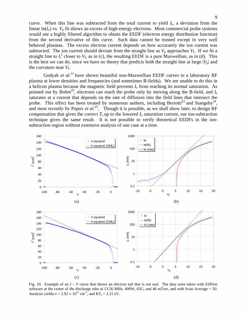
9curve. When this line was subtracted from the total current to yield Ie, a deviation from the linear ln(Ie) vs. Vp fit shows an excess of high-energy electrons. Most commercial probe systems would use a highly filtered algorithm to obtain the EEDF (electron energy distribution function) from the second derivative of this curve. Such data cannot be trusted except in very well behaved plasmas. The excess electron current depends on how accurately the ion current was subtracted. The ion current should deviate from the straight line as Vp approaches Vf. If we fit a straight line to Ii

2 closer to Vf, as in (c), the resulting EEDF is a pure Maxwellian, as in (d). This is the best we can do, since we have no theory that predicts both the straight line at large |Vp| and the curvature near Vf.

Godyak et al.21 have shown beautiful non-Maxwellian EEDF curves in a laboratory RF plasma at lower densities and frequencies (and sometimes B-fields). We are unable to do this in a helicon plasma because the magnetic field prevents Ie from reaching its normal saturation. As pointed out by Bohm22, electrons can reach the probe only by moving along the B-field, and Ie saturates at a current that depends on the rate of diffusion into the field lines that intersect the probe. This effect has been treated by numerous authors, including Bertotti23 and Stangeby24, and most recently by Popov et al.25, Though it is possible, as we shall show later, to design RF compensation that gives the correct Te up to the lowered Ie saturation current, our ion-subtraction technique gives the same result. It is not possible to verify theoretical EEDFs in the ion-subtraction region without extensive analysis of one case at a time.

(a) (b)

0

20

40

60

80

100

120

140

160

180

-100 -80 -60 -40 -20 0V

I2 (

mA

)2

Ii squared

Ii squared (OML)

0.1

1

10

100

1000

-10 -5 0 5 10 15 20Vp

I e (

mA

)

Ie

Ie(fit)

Ie (raw)

(c) (d)

Fig. 10. Example of an I – V curve that shows an electron tail that is not real. The data were taken with ESPion software at the center of the discharge tube at 13.56 MHz, 400W, 65G, and 46 mTorr, and with Scan Average = 50. Analysis yields n = 2.92 × 1012 cm-3, and KTe = 2.21 eV.

0.1

1

10

100

1000

-10 -5 0 5 10 15 20Vp

I e (

mA

)

Ie

Ie(fit)

Ie (raw)

0

20

40

60

80

100

120

140

160

-100 -80 -60 -40 -20 0V

I2 (

mA

)2

Ii squared

Ii squared (OML)

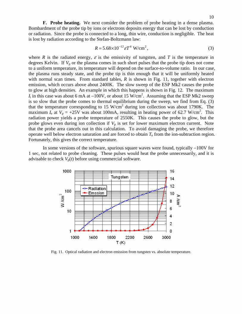
10 F. Probe heating. We next consider the problem of probe heating in a dense plasma. Bombardment of the probe tip by ions or electrons deposits energy that can be lost by conduction or radiation. Since the probe is connected to a long, thin wire, conduction is negligible. The heat is lost by radiation according to the Stefan-Boltzmann law:

12 4 25.68 10 W/cmR Tε−= × , (3)

where R is the radiated energy, ε is the emissivity of tungsten, and T is the temperature in degrees Kelvin. If Vp or the plasma comes in such short pulses that the probe tip does not come to a uniform temperature, its temperature will depend on the surface-to-volume ratio. In our case, the plasma runs steady state, and the probe tip is thin enough that it will be uniformly heated with normal scan times. From standard tables, R is shown in Fig. 11, together with electron emission, which occurs above about 2400K. The slow sweep of the ESP Mk2 causes the probe to glow at high densities. An example in which this happens is shown in Fig. 12. The maximum Ii in this case was about 6 mA at −100V, or about 15 W/cm2. Assuming that the ESP Mk2 sweep is so slow that the probe comes to thermal equilibrium during the sweep, we find from Eq. (3) that the temperature corresponding to 15 W/cm2 during ion collection was about 1790K. The maximum Ie at Vp = +25V was about 100mA, resulting in heating power of 62.7 W/cm2. This radiation power yields a probe temperature of 2550K. This causes the probe to glow, but the probe glows even during ion collection if Vp is set for lower maximum electron current. Note that the probe area cancels out in this calculation. To avoid damaging the probe, we therefore operate well below electron saturation and are forced to obtain Te from the ion-subtraction region. Fortunately, this gives the correct temperature.

In some versions of the software, spurious square waves were found, typically −100V for 1 sec, not related to probe cleaning. These pulses would heat the probe unnecessarily, and it is advisable to check Vp(t) before using commercial software.

Fig. 11. Optical radiation and electron emission from tungsten vs. absolute temperature.

11

0

10

20

30

40

-100 -80 -60 -40 -20 0V

I2 (

mA

)2Ii squared

Ii squared (OML)

0.01

0.1

1

10

100

1000

0 5 10 15 20 25V

I e (

mA

)

Ie

Ie(fit)

Ie (raw)

Fig 12. Ion and electron curves of a case when the probe glows. ESP Mk2 software, 13.56 MHz, 60G, 400W, 15

mTorr, n = 1.65 × 1012 cm-3, KTe = 2.72 eV.

G. Operation with short scans. To collect higher electron current, we changed the software to ESPion, which takes the data in bunches of fast sweeps, as shown in Fig. 6b. Remember that ESPion has a Scan Average (SA) setting which set the number of scans in each bunch that are averaged. Without going into details, we have checked that the ESPion and ESP Mk2 systems give identical results in most cases, even though ESPion’s ion curves are not as smooth if SA is less than about 50. This was instrumental: the discharge itself was checked to be completely free of low-frequency oscillations. The main difference in ESPion is in the 1000 mA current range setting, which is not available in the ESP Mk2. The 1000 mA range in ESPion gives correct currents at 13.56 MHz, but currents that are too high at 27 MHz. This is probably caused by the increased inductance of the 1-Ω current-measuring resistor at 27 MHz, an effect which could exist in other systems as well. Note that the ion current at high |Vp| dips below the straight line in Fig. 12. This is likely due to the formation of an absorption radius at high densities. At very low densities an opposite, upward curvature has been observed, which could be caused by large sheath expansion on a short probe, which then begins at act like a spherical probe.

H. Electron emission with scan bunches. Figure 13 shows the ESPion data of the same discharge as in Fig. 12, taken up to Vp = +20V with SA = 10 and with the same 100-mA current range and 200 points per scan. The derived n and KTe values are in reasonable agreement with those of Fig. 12. The probe does not glow. The pulse bunch is short enough that the probe tip does not come to thermal equilibrium and has enough heat capacity to absorb the particle energy without being heated to emit observable light.

Fig. 13. Ion and electron curves of the plasma of Fig. 12, but taken with ESPion software. The derived n is 1.57 ×

1012 cm-3, and KTe = 2.6 eV.

0.01

0.1

1

10

100

1000

-10 0 10 20V

I e (

mA

)

Ie

Ie(fit)

Ie (raw)

0

10

20

30

40

-100 -80 -60 -40 -20 0V

I2 (

mA

)2

Ii squared

Ii squared (OML)

12 If now the upper limit of ESPion sweep voltage is raised, the probe will first be driven to a glowing temperature, then start to emit electrons. Figure 14 shows that electron emission can also affect ion saturation current in scan bunches. The interaction occurs because the probe is heated by Ie during the first few scans of the bunch. On subsequent scans, Ii is measured while the probe is emitting electrons. In Fig. 14a, a small amount of emission occurs as Vmax (the maximum Vp in each scan) is raised from 15 to 50V, with SA = 50. At Vmax = 50V, n drops because SA was reduced to 25 to reduce the heating. At Vmax = 60, n takes a big jump as SA is increased back to 50. Figure 14b shows the same data on a smaller scale to show the Vmax = 70V point with SA = 50. The probe is in total emission, and n is greatly affected by electron emission. The Vmax = 70V I2 – V curve (not shown) looks exactly like that in Fig. 12 but with much higher values. The Ie curve for that case is shown in Fig. 15. At the Vmax = 70V point (actually 67V), Ie was 46.8mA. This corresponds to 786 W/cm2 and a probe temperature of 4800K, according to Eq. (3). Clearly, the scans were fast enough that the probe did not reach thermal equilibrium.

10

12

14

16

18

20

0 20 40 60 80Vmax

n11 SA = 25

20

5050

50

0

10

20

30

40

50

60

0 20 40 60 80Vmax

n1

1

(a) (b)

Fig. 14. (a) Ion-derived densities vs. maximum positive Vp on each scan using ESPion. (b) Same as (a) but extended to Vmax = 70V on a different scale. 400W at 13.56 MHz, 65G, 15 mTorr; probe at center of discharge.

Fig. 15. Electron curves for the Vmax = +70V case shown on two scales. At 2.87eV, KTe was normal.

I. Absence of transition region. In Fig. 15, electron saturation occurs at such low Vp that Te could be obtained only from the ion-subtraction region, which extends nearly to Ie saturation. Setting Vmax higher than 25V is not necessary, since Ie is already saturated there. Te can be measured without overheating the probe. This unusual situation is caused by the orientation of the probe along a strong B-field.

J. Design of compensation electrode. An attempt was made to improve RF compensation by making a larger CE. The sheath capacitance of the CE should be much larger

0.1

1

10

100

1000

0 20 40 60V

I e (

mA

)

Ie

Ie(fit)

Ie (raw)

0.1

1

10

100

1000

0 5 10 15 20 25 30V

I e (

mA

)

Ie

Ie(fit)

Ie (raw)

13than that of the probe tip. The sheath capacitance Csh has been calculated by many authors; for instance, by Godyak and Sternberg26. Using their method, Chen27 gave Csh as

½

01/2½

1 (1 2 )

2 (1 2 ) 2

sh

D

C e

A e

η

η

ε ηλ η

− −

−

+ −= + + −

, (4)

where A is the probe area and η the sheath drop normalized to KTe. With A given by the area of the CE, the impedance of the sheath on the CE is given by |Zx| = 1/ωCsh. This impedance then forms an RF voltage divider with the impedance |Zck| of the choke chain. The requirement for the RF amplitude rfV to be reduced to a small fraction of KTe is then given by

1rf rfx x

e ck x e ck

eV eVZ Z

KT Z Z KT Z≈ <<

+

(5)

Using the value of rfV from Fig. 8 and that of |Zck| from Fig. 5, we then determined that our CE

should be 2 cm long instead of 1 cm. Such a CE was made and inserted, but it could not be withdrawn into the 18-in. hole without touching ground and was so large compared with the small discharge that no good data could be taken with it. In this exercise we also tried leaving the connecting wire of a 1.2-cm long CE unshielded, thus requiring only one thin alumina tube to be inserted into the discharge. This made no difference, and Fig. 15, for instance, was taken with such a bare wire.

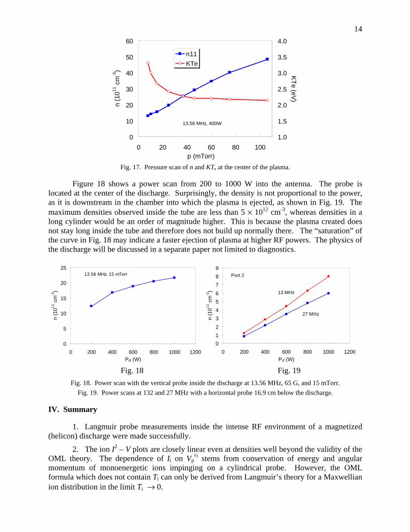
K. Examples of data. Here we give examples of data taken of the discharge inside the tube using the techniques described above. The axial profile of density is shown in Fig. 16 in relation to the tube. The CE was 1.2 cm long, connected to the probe with a bare wire. The farthest point reached by the vertical probe is only a few mm above a horizontal probe with a very large CE. The densities measured with the two probes were in absolute agreement. Figure 17 shows the pressure dependence of density at the center of the discharge under the same conditions. The electron temperature falls with increasing pressure in agreement with theory.

0

4

8

12

16

0 2 4 6 8 10 12z (cm)

n11

400W, 13.56 MHz, 15 mTorr

Fig. 16. Axial density profile in units of 1011 cm-3 in a 13.56-MHz helicon discharge at 400W, 15 mTorr of Ar, and

a 65G average B-field.

14

0

10

20

30

40

50

60

0 20 40 60 80 100p (mTorr)

n (1

01

1 c

m-3

)

1.0

1.5

2.0

2.5

3.0

3.5

4.0

KT

e (eV)

n11

KTe

13.56 MHz, 400W

Fig. 17. Pressure scan of n and KTe at the center of the plasma.

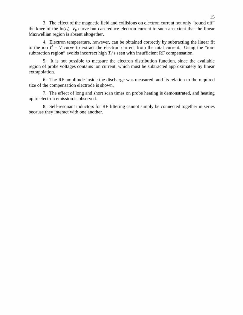
Figure 18 shows a power scan from 200 to 1000 W into the antenna. The probe is located at the center of the discharge. Surprisingly, the density is not proportional to the power, as it is downstream in the chamber into which the plasma is ejected, as shown in Fig. 19. The maximum densities observed inside the tube are less than 5 × 1012 cm-3, whereas densities in a long cylinder would be an order of magnitude higher. This is because the plasma created does not stay long inside the tube and therefore does not build up normally there. The “saturation” of the curve in Fig. 18 may indicate a faster ejection of plasma at higher RF powers. The physics of the discharge will be discussed in a separate paper not limited to diagnostics.

0

5

10

15

20

25

0 200 400 600 800 1000 1200Prf (W)

n (1

011

cm

-3)

13.56 MHz, 15 mTorr

0

1

2

3

4

5

6

7

8

9

0 200 400 600 800 1000 1200

Prf (W)

n (1

01

1 c

m-3

) 13 MHz

27 MHz

Port 2

Fig. 18 Fig. 19

Fig. 18. Power scan with the vertical probe inside the discharge at 13.56 MHz, 65 G, and 15 mTorr.

Fig. 19. Power scans at 132 and 27 MHz with a horizontal probe 16.9 cm below the discharge.

IV. Summary

1. Langmuir probe measurements inside the intense RF environment of a magnetized (helicon) discharge were made successfully.

2. The ion I2 – V plots are closely linear even at densities well beyond the validity of the OML theory. The dependence of Ii on Vp

½ stems from conservation of energy and angular momentum of monoenergetic ions impinging on a cylindrical probe. However, the OML formula which does not contain Ti can only be derived from Langmuir’s theory for a Maxwellian ion distribution in the limit Ti → 0.

15 3. The effect of the magnetic field and collisions on electron current not only “round off” the knee of the ln(Ie)−Vp curve but can reduce electron current to such an extent that the linear Maxwellian region is absent altogether.

4. Electron temperature, however, can be obtained correctly by subtracting the linear fit to the ion I2 – V curve to extract the electron current from the total current. Using the “ion-subtraction region” avoids incorrect high Te’s seen with insufficient RF compensation.

5. It is not possible to measure the electron distribution function, since the available region of probe voltages contains ion current, which must be subtracted approximately by linear extrapolation.

6. The RF amplitude inside the discharge was measured, and its relation to the required size of the compensation electrode is shown.

7. The effect of long and short scan times on probe heating is demonstrated, and heating up to electron emission is observed.

8. Self-resonant inductors for RF filtering cannot simply be connected together in series because they interact with one another.

16

REFERENCES 1 S. Klagge and M. Maass, Beiträge aus der Plasmaphysik 23, 355 (1983). 2 N. Hershkowitz, How Langmuir Probes Work, in Plasma Diagnostics, Vol. 1, ed. by O. Auciello and D.L. Flamm

(Academic Prsss, San Diego, CA, 1989), p.169. 3 M.A. Lieberman and A.J. Lichtenberg, Principles of Plasma Discharges and Materials Processing, 2nd ed. (Wiley-

Interscience, Hoboken, NJ, 2005), p. 202. 4 H.M. Mott-Smith and I. Langmuir, Phys. Rev. 28, 727 (1926). 5 J.E. Allen, R.L.F. Boyd, and P. Reynolds, Proc. Phys. Soc. (London) B 70, 297 (1957). 6 I.B. Bernstein, and I.N. Rabinowitz, Phys. Fluids 2, 112 (1959). 7 J.G. Laframboise, J.G. Univ. Toronto Inst. Aerospace Studies Rept. 100 (1966), unpublished.. 8 F.F. Chen, J. Nucl. Energy, Pt. C 7, 47 (1965). 9 F.F. Chen, Phys. Plasmas 8, 3029 (2001). 10 F.F. Chen, J. D. Evans, and W. Zawalski, Calibration of Langmuir probes against microwaves and plasma

oscillation probes, submitted to Plasma Sources Sci. Technol. (2012). 11 F.F. Chen, Plasma Sources Sci. Technol. 18, 035012 (2009). 12 http://www.hidenanalytical.com/index.php/en/product-catalog/51-plasma-characterisation/80-hiden-espion-

advanced-langmuir-probe-for-plasma-diagnostics 13 www.impedans.com 14 http://www.pnasol.com 15 F.F. Chen and H. Torreblanca, Plasma Phys. Control. Fusion 49, A81 (2007). 16 F.F. Chen and H. Torreblanca, Phys. Plasmas 16, 057102 (2009). 17 F.F. Chen and H. Torreblanca, IEEE Trans. Plasma Sci. 39, No. 11, 2452 (2011). 18 F.F. Chen, Phys. Plasmas 10, 2586 (2003). 19 I.D. Sudit and F.F. Chen, Plasma Sources Sci. Technol. 3, 162 (1994). 20 F.F. Chen, J.Appl. Phys. 36, 675 (1965). 21 V. A. Godyak and V. I. Demidov, J. Phys. D: Appl. Phys. 44, 233001 (2011). 22 D. Bohm, E.H.S. Burhop,and H.S.W. Massey, in Characteristics of EIectrical Discharges in MagneticF ields, ed.

by A. Guthrie and R. K. Wakerling (McGraw-Hill, New York, 1949). 23 B. Bertotti, Phys. Fluids 4, 1047 (1961). 24 P. C. Stangeby, J. Phys. D. 15, 1007 (1982). 25 Tsv K. Popov, P. Ivanova, M. Dimitrova, J. Kovacic, T. Gyergyek, and M. Cercek4, Plasma Sources Sci. Technol.

21, 025004 (2012). 26 V.A. Godyak and N. Sternberg, Proc. 20th Intl. Conf. on Phenomena in Ionized Gases, Barga, Italy (1991), p. 661. 27 F.F. Chen, Plasma Sources Sci. Technol. 15, 773 (2006).