1--ul-u ltA4 200r

Evolution r ip. zz.s--z.3.5--

DOUGLAS J. FUTUYMAState University of New York at Stony Brook

Chapter 19, "Evolution of Genes and Genomes"by Scott V. Edwards, Harvard University

Chapter 20, "Evolution and Development"by John R. True, State University of New York at Stony Brook

VASINAUER ASSOCIATES, INC. • PublishersSunderland, Massachusetts U.S.A.

10Genetic Drift:Evolution at Random

ne of the first and most

important lessons a

student of science learns

is that many words have very

different meanings in a scientific

context than in everyday speech.

The word "chance" is a good ex-

ample. Many nonscientists think

that evolution occurs "by

chance." What they mean is that

evolution occurs without pur-

pose or goal. But by this token,

everything in the natural

world—chemical reactions,

weather, planetary movements,

earthquakes—happens by

chance, for none of these phe-

nomena have purposes. In fact, scientists consider purposes or goals to be

unique to human thought, and they do not view any natural phenomena

as purposeful. But scientists don't view chemical reactions or planetary

movements as chance events, either—because in science, "chance" has a

very different meaning.

Although the meaning of "chance" is a complex philosophical issue,

scientists use chance, or randomness, to mean that when physical causes

can result in any of several outcomes, we cannot predict what the outcome

will be in any particular case. Nonetheless, we may be able to specify

Polymorphism in snails.Populations of the Europeanland snail Cepaea nemoralis aregenetically polymorphic forbackground color and for thenumber and width of the darkbands on their shells. Extensiveresearch has shown that bothgenetic drift and natural selec-tion affect the allele frequenciesfor these traits. (Photo by D.McIntyre.)

226 CHAPTER 10

the probability, and thus the frequency, of one or another outcome. Although we cannot pre-dict the sex of someone's next child, we can say with considerable certainty that there isa probability of 0.5 that it will be a daughter.

Almost all phenomena are affected simultaneously by both chance (unpredictable) andnonrandom, or DETERMINISTIC (predictable), factors. Any of us may experience a car acci-dent due to the unpredictable behavior of other drivers, but we are predictably more likelto do so if we drive after drinking. So it is with evolution. As we will see in the next chater, natural selection is a deterministic, nonrandom process. But at the same time, theare important random processes in evolution, including mutation (as discussed in Chap-ter 8) and random fluctuations in the frequencies of alleles or haplotypes: the processrandom genetic drift.

Genetic drift and natural selection are the two most important causes of allele substi-tution—that is, of evolutionary change—in populations. Genetic drift occurs in all natu-ral populations because, unlike ideal populations at Hardy-Weinberg equilibrium, nat-ural populations are finite in size. Random fluctuations in allele frequencies can result inthe replacement of old alleles by new ones, resulting in nonadaptive evolution. That is,while natural selection results in adaptation, genetic drift does not—so this process is notresponsible for those anatomical, physiological, and behavioral features of organisms thatequip them for reproduction and survival. Genetic drift nevertheless has many importantconsequences, especially at the molecular genetic level: it appears to account for much ofthe difference in DNA sequences among species.

Because all populations are finite, alleles at all loci are potentially subject to randomgenetic drift—but all are not necessarily subject to natural selection. For this reason, andbecause the expected effects of genetic drift can be mathematically described with someprecision, some evolutionary geneticists hold the opinion that genetic drift should be the"null hypothesis" used to explain an evolutionary observation unless there is positive ev-idence of natural selection or some other factor. This perspective is analogous to the "nullhypothesis" in statistics: the hypothesis that the data do not depart from those expectedon the basis of chance alone.* According to this view, we should not assume that a char-acteristic, or a difference between populations or species, is adaptive or has evolved bynatural selection unless there is evidence for this conclusion.

The theory of genetic drift, much of which was developed by the American geneticistSewall Wright starting in the 1930s, and by the Japanese geneticist Motoo Kimura start-ing in the 1950s, includes some of the most highly refined mathematical models in biol-ogy. (But fear not! We shall skirt around almost all the math.) We will first explore the the-ory and then see how it explains data from real organisms. In our discussion of the theoryof genetic drift, we will describe random fluctuations in the frequencies (proportions)of two or more kinds of self-reproducing entities that do not differ on average (or differvery little) in reproductive success (fitness). For the purposes of this chapter, those enti-ties are alleles. But the theory applies to any other self-replicating entities, such as chro-mosomes, asexually reproducing genotypes, or even species.

The Theory of Genetic Drift

Genetic drift as sampling error

That chance should affect allele frequencies is readily understandable. Imagine, for exam-ple, that a single mutation, A2, appears in a large population that is otherwise Al . If thepopulation size is stable, each mating pair leaves an average of two progeny that surviveto reproductive age. From the single mating A1A1 x A 1A2 (for there is only one copy of A2),

the probability that one surviving offspring will be A1A1 is 1/2; therefore, the probability

*For example, if we measure height in several samples of people, the null hypothesis is that the observedmeans differ from one another only because of random sampling, and that the parametric means of the popu-lations from which the samples were drawn do not differ. A statistical test, such as a t-test or analysis of vari-ance, is designed to show whether or not the null hypothesis can be rejected. It will be rejected if the samplemeans differ more than would be expected if samples had been randomly drawn from a single population.

GENETIC DRIFT: EVOLUTION AT RANDOM 227

that two surviving progeny will both be A iA i is 1/2 x 1/2 = 1/4—which is the probability that

the A2 allele will be immediately lost from the population. We may assume that matingpairs vary at random, around the mean, in the number of surviving offspring they leave(0, 1, 2, 3 ... ). In that case, as the pioneering population geneticist Ronald Fisher calculated,the probability that A2 will be lost, averaged over the population, is 0.368. He went on tocalculate that after the passage of 127 generations, the cumulative probability that the al-lele will be lost is 0.985. This probability, he found, is not greatly different if the new mu-tation confers a slight advantage: as long as it is rare, it is likely to be lost, just by chance.

In this example, the frequency of an allele can change (in this instance, to zero from afrequency very near zero) because the one or few copies of the A2 allele may happen notto be included in those gametes that unite into zygotes, or may happen not to be carriedby the offspring that survive to reproductive age. The genes included in any generation,whether in newly formed zygotes or in offspring that survive to reproduce, are a sampleof the genes carried by the previous generation. Any sample is subject to random varia-tion, or sampling error. In other words, the proportions of different kinds of items (in this

case, Al and A2 alleles) in a sample are likely to differ, by chance, from the proportions inthe set of items from which the sample is drawn.

Imagine, for example, a population of land snails (Cepaea nemoralis; see the photographthat opens this chapter) in which (for the sake of argument) offspring inherit exactly thebrown or yellow color of their mothers. Suppose 50 snails of each color inhabit a cow pas-ture. (The proportion of yellow snails is p = 0.50.) If 2 yellow and 4 brown snails arestepped on by cows, p will change to 0.511. Since it is unlikely that a snail's color affectsthe chance of its being squashed by cows, the change might just as well have been the re-verse, and indeed, it may well be the reverse in another pasture, or in this pasture in thenext generation. In this random process, the chances of increase or decrease in the pro-portion of yellow snails are equal in each generation, so the proportion will fluctuate. Butan increase of, say, 1 percent in one generation need not be compensated by an equal de-crease in a later generation—in fact, since this process is random, it is very unlikely thatit will be. Therefore the proportion of yellow snails will wander over time, eventually end-ing up near, and finally at, one of the two possible limits: 0 and 1.0. It seems reasonable,too, that if the population should start out with, say, 80 percent brown and 20 percent yel-low snails, it is more likely that the proportion of yellow will wander to zero than to 100percent. In fact, the probability of yellow being lost from the population is exactly 0.20.Conversely, the probability that brown will reach 100 percent—that is, that it will befixed—is 0.80.

Coalescence

The concept of random genetic drift is so important that we will take two tacks in devel-oping the idea. Figure 10.1 shows a hypothetical, but realistic, history of gene lineages. First,imagine the figure as depicting lineages of individual asexual organisms, such as bacteria,rather than genes. We know from our own experience that not all members of our parents'or grandparents' generations had equal numbers of descendants; some had none. Figure10.1 diagrams this familiar fact. We note that the individuals in generation t (at the right ofthe figure) are the progeny of only some of those that existed in the previous generation(t - 1): purely by chance, some individuals in generation t -1 failed to leave descendants.Likewise, the population at generation t -1 stems from only some of those individuals thatexisted in generation t - 2, and similarly back to the original population at time 0.

Now think of the objects in Figure 10.1 as copies of genes at a locus, in either a sexualor an asexual population. Figure 10.1 shows that as time goes on, more and more of theoriginal gene lineages become extinct, so that the population consists of descendants offewer and fewer of the original gene copies. In fact, if we look backward rather than for-

ward in time, all the gene copies in the population ultimately are descended from a single an-cestral gene copy, because given long enough, all other original gene lineages become ex-

tinct. The genealogy of the genes in the present population is said to coalesce back to a

single common ancestor. Because that ancestor represents one of the several original al-

leles, the population's genes, descended entirely from that ancestral gene copy, must even-

6-1

0--

A,

A,

A,

A,

Ai

A1

A1

Al

Al

Ai

A1

•

CHAPTER 10228

Figure 10.1 A possible history of descent of gene copies in a popula-tion that begins (at time 0, at left) with 15 copies, representing two alle-les. Each gene copy has 0, 1, or 2 descendants in the next generation.The gene copies present at time t (at right) are all descended from (coa-lesce to) a single ancestral copy, which happens to be an A2 allele (thelineage shown in red). Gene lineages descended from all other genecopies have become extinct. If the failure of gene copies to leave descen-dants is random, then the gene copies at time t could equally likelyhave descended from any of the original gene copies present at time 0.(After Hartl and Clark 1989.)

nBy time t, all copiesof the gene present tually become monomorphic: one or the otherin the population of the original alleles becomes fixed (reaches aare descended from

singleato)to(coalesce frequency of 1.00). The smaller the population,( ancestral gene copy. the more rapidly all gene copies in the current

population coalesce back to a single ancestralcopy, since it takes longer for many than for few

gene lineages to become extinct by chance.In our example, all gene copies have descended from a copy of an

A2 allele, but because this is a random process, A1 might well have been

the "lucky" allele if the sequence of random events had been different.If, in the generation that included the single common ancestor of all oftoday's gene copies, A 1 and A2 had been equally frequent (p = q = 0.5),then it is equally likely that the ancestral gene copy would have beenA1 or A2; but if A1 had had a frequency of 0.9 in that generation, thenthe probability is 0.9 that the ancestral gene would have been an A 1 al-lele. Our analysis therefore shows that by chance, a population will eventu-ally become monomorphic for one allele or the other, and that the probability

that allele A1 will be fixed, rather than another allele, equals the initial frequency of Al.According to this analysis, for example, all the mitochondria of the entire human pop-

ulation are descended from the mitochondria carried by a single woman, who has beencalled "mitochondrial Eve," at some time in the past. (Mitochondria are transmitted onlythrough eggs.) This does not mean, however, that the population had only one woman atthat time: "mitochondrial Eve" happened to be the one among many women to whom allmitochondria trace their ancestry (in a pattern like that seen in Figure 10.1). Variousclear genes likewise are descended from single gene copies in the past that were carriedby many different members of the ancestral human population.

If this process occurs in a large number of independent, non-interbreeding populations,each with the same initial number of copies of each of two alleles at, say, locus A, then wewould expect a fraction p of the populations to become fixed for A 1 and a fraction 1– p tobecome fixed for A2 . Thus the genetic composition of the populations would diverge bychance. If the original populations had each contained three (or more) different alleles,rather than two, each of those alleles would become fixed in some of the populations, witha probability equal to its initial frequency (say, p1). 41.

As allele frequencies in a population change by genetic drift, so do the genotype fre-quencies, which conform to Hardy-Weinberg equilibrium among the new zygotes in eachgeneration. If, for example, the frequencies p and q (that is, p and 1 – p) of alleles A1 and

A 2 change from 0.5: 0.5 to 0.45: 0.55, then the frequencies of genotypes A 1A 1 , A 1A2, and

A2A2 change from 0.25:0.50:0.25 to 0.2025:0.4950:0.3025. As was described in Chapter 9,the frequency of heterozygotes, H, declines as one of the allele frequencies shifts closer to1 (and the other moves toward 0):

(1

Time

H = 2p(1 – p)

Bear in mind that this model, as developed so far, includes only the effects of randomgenetic drift. It assumes that other evolutionary processes—namely, mutation, gene flow,and natural selection—do not operate. Thus the model does not describe the evolution of

A,

A,

e—C

c Initially (time 0) the populationhas 15 copies of gene A.

Most of the copies becomeextinct over several generations.

V

GENETIC DRIFT: EVOLUTION AT RANDOM 229

aptive traits—those that evolve by natural selection. We will incorporate natural se-lection in the following chapters.

Random fluctuations in allele frequenciesLet us take another, more traditional, approach to the concept of random genetic drift. As-sume that the frequencies of alleles A 1 and A2 are p and q in each of many independentpopulations, each with N breeding individuals (representing 2N gene copies in a diploidspecies) . Small independent populations are sometimes called demes, and an ensembleof such populations may be termed a metapopulation. As before, we assume that thegenotypes do not differ, on average, in survival or reproductive success—that is, the alle-les are neutral with respect to fitness.

In each generation, the large number of newborn zygotes is reduced to N individualsby the time the next generation breeds, by mortality that is random with respect to geno-type. By sampling error, the proportion of A1 (p) among the survivors may change. Thenew p (call it p') could take on any possible value from 0 to 1.0, just as the proportion ofheads among N tossed coins could, in principle, range from all heads to all tails. The prob-ability of each possible value—whether it be the proportion of heads or the proportion ofA 1 allele copies—can be calculated from the binomial theorem, generating a PROBABILITY

DISTRIBUTION. Among a large number of demes, the new allele frequency (p') will vary, bychance, around a mean—namely, the original frequency, p.

Now if we trace one of the demes, in which p has changed from 0.5 to, say, 0.47, we seethat in the following generation, it will change again from 0.47 to some other value, eitherhigher or lower with equal probability. This process of random fluctuation continues overtime. Since no stabilizing force returns the allele frequency toward 0.5, p will eventuallywander (drift) either to 0 or to 1: the allele is either lost or fixed. (Once the frequency of anallele has reached either 0 or 1, it cannot change unless another allele is introduced intothe population, either by mutation or by gene flow from another population.) The allelefrequency describes a random walk, analogous to a New Year's Eve reveler staggeringalong a very long train platform with a railroad track on either side: if he is so drunk thathe doesn't compensate steps toward one side with steps toward the other, he will even-tually fall off the edge of the platform onto one of the two tracks, if the platform is longenough (Figure 10.2).

Just as an allele's frequency may increase by chance in some demes from one genera-tion to the next, it may decrease in other demes. As a result, allele frequencies may varyamong the demes. The variance in allele frequency among the demes continues to increasefrom generation to generation (Figure 10.3). Some demes reach p = 0 or p = 1 and can nolonger change. Among those in which fixation of one or the other allele has not yet oc-curred, the allele frequencies continue to spread out, with all frequencies between 0 and1 eventually becoming equally likely (Figure 10.4). Those that approach 0 or 1 tend to "fallover the edge," so the number of populations fixed for one or another allele continuesto increase, until all demes in the metapopulation have become fixed. Thus demes thatinitially are genetically identical evolve by chance to have different genetic constitutions.(Remember, though, that we are assuming that the alleles have identicaleffects on fitness—that is, that they are neutral.)

Figure 10.2 A "random walk" (or"drunkard's walk"). The reveler even-tually falls off the platform if he is toofar gone to steer a course toward themiddle. The edges of the platform ("0"and "1") represent loss and fixation ofart allele, respectively.

Fixation

Loss-4-- 0

Oscillations are larger, andalleles are more rapidly fixedor lost, in small populations...

(B)

1.0 50 individuals, 100 gene copies

8

12

16

20

Generation

9 individuals, 18 gene copies

230 CHAPTER 10

Figure 10.3 Computer simulations of random geneticpopulations of (A) 9 diploid individuals (2N 18 gene cand (B) 50 diploid individuals (2N = 100 gene copies). Eachtraces the frequency (p) of one allele for 20 generations. Eacpanel shows allele frequency changes in 20 replicate popuiations, all of which begin at p = 0.5 (i.e., half the gene copiesA1 and half A2). (After Hartl and Clark 1989.)

c ..than in

— .111 -1111111°44°64-111t. 11. .4411111111144.

larger ones.0.8

cr

..1.0.-dittN04400

0.4 11110.-

0.2

Initial allele frequencyis 0.5 in all populations.

t 0.6

t = 0.1N generations Each curve representsthe distribution of allelefrequencies amongseveral populations,each of size N, that allbegan with the samefrequency (p = 0.5).

4 8 12

Generation

16

(...or upward to 1.

t 05N

16.VriNiak.

0

0.5

(B)

Allele frequency

Allele lost

t

0

0.5

Allele frequency

Allele frequencies driftdownward to 0...

S.

At time r = 2Ngenerations, allallele frequenciesbetween 0 and 1are equally likely.

1.0

Figure 10.4 Changes in the probability that an allele will have various possble frequencies as genetic drift proceeds over time. (A) Each curve shows theprobability distribution of allele frequencies between 0 and 1 at different timThe number of generations that elapse (t) is measured in units of the initial porulation size (N). For example, if the population begins with N = 50 individuat = 2N represents the frequency distribution after 100 generations. The probalty distribution after t = 0.1N generations is shown by the uppermost curve. Tcurve may be thought of as the distribution of allele frequencies among severpopulations, each of size N, that began with the same allele frequency. With t

passage of generations, the curve becomes lower and broader as the allele frt-quencies in all populations drift toward either 0 or 1. At t = 2N generations,allele frequencies between 0 and 1 are equally likely. (This panel does not shethe proportion of populations in which the allele has been fixed or lost.) (B)proportion of populations with different allele frequencies after t = 2N generalions have elapsed, including populations in which the allele has been fixed(p = 1) or lost (p = 0). The proportion of populations in which the allele is losfixed increases at the rate of 1/(4N) per generation, and each allele frequenc)class between 0 and 1 decreases at the rate of 1/(2N) per generation. (A afterKimura 1955; B after Wright 1931.)

12N

Allele fixed

0

(A)

GENETIC DRIFT: EVOLUTION AT RANDOM 231

Evolution by Genetic Drift

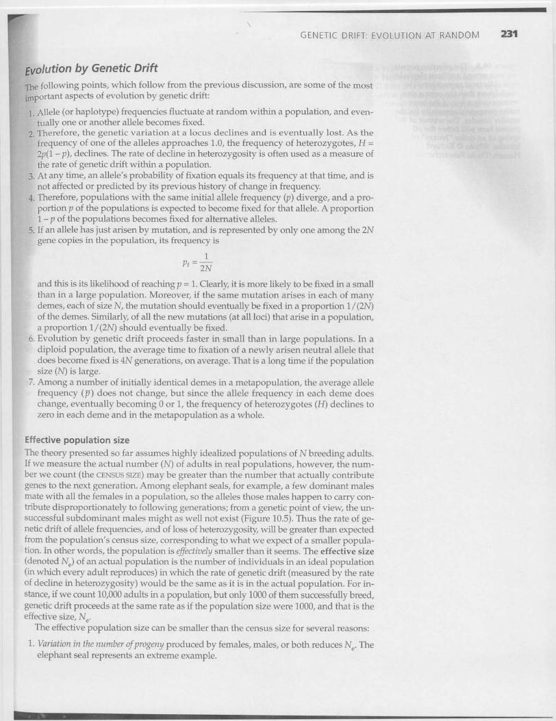
The following points, which follow from the previous discussion, are some of the mostimportant aspects of evolution by genetic drift:

1. Allele (or haplotype) frequencies fluctuate at random within a population, and even-tually one or another allele becomes fixed.

2. Therefore, the genetic variation at a locus declines and is eventually lost. As thefrequency of one of the alleles approaches 1.0, the frequency of heterozygotes, H =2p(1 — p), declines. The rate of decline in heterozygosity is often used as a measure ofthe rate of genetic drift within a population.

3. At any time, an allele's probability of fixation equals its frequency at that time, and isnot affected or predicted by its previous history of change in frequency

4. Therefore, populations with the same initial allele frequency (p) diverge, and a pro-portion p of the populations is expected to become fixed for that allele. A proportion1— p of the populations becomes fixed for alternative alleles.

5. If an allele has just arisen by mutation, and is represented by only one among the 2Ngene copies in the population, its frequency is

1Pt — 2N2N

and this is its likelihood of reaching p = 1. Clearly, it is more likely to be fixed in a smallthan in a large population. Moreover, if the same mutation arises in each of manydemes, each of size N, the mutation should eventually be fixed in a proportion 1 /(2N)of the demes. Similarly, of all the new mutations (at all loci) that arise in a population,a proportion 1 / (2N) should eventually be fixed.

6. Evolution by genetic drift proceeds faster in small than in large populations. In adiploid population, the average time to fixation of a newly arisen neutral allele thatdoes become fixed is 4N generations, on average. That is a long time if the populationsize (N) is large.

7. Among a number of initially identical demes in a metapopulation, the average allelefrequency (p) does not change, but since the allele frequency in each deme doeschange, eventually becoming 0 or 1, the frequency of heterozygotes (H) declines tozero in each deme and in the metapopulation as a whole.

Effective population sizeThe theory presented so far assumes highly idealized populations of N breeding adults.If we measure the actual number (N) of adults in real populations, however, the num-ber we count (the CENSUS SIZE) may be greater than the number that actually contributegenes to the next generation. Among elephant seals, for example, a few dominant malesmate with all the females in a population, so the alleles those males happen to carry con-tribute disproportionately to following generations; from a genetic point of view, the un-successful subdominant males might as well not exist (Figure 10.5). Thus the rate of ge-netic drift of allele frequencies, and of loss of heterozygosity, will be greater than expectedfrom the population's census size, corresponding to what we expect of a smaller popula-tion. In other words, the population is effectively smaller than it seems. The effective size(denoted Ne) of an actual population is the number of individuals in an ideal population(in which every adult reproduces) in which the rate of genetic drift (measured by the rateof decline in heterozygosity) would be the same as it is in the actual population. For in-stance, if we count 10,000 adults in a population, but only 1000 of them successfully breed,genetic drift proceeds at the same rate as if the population size were 1000, and that is theeffective size, Ne.

The effective population size can be smaller than the census size for several reasons:

1. Variation in the number of progeny produced by females, males, or both reduces N,. Theelephant seal represents an extreme example.

232 CHAPTER 10

Figure 10.5 The effective popula-tion size among northern elephantseals (Mirounga angustirostris) ismuch lower than the census sizebecause only a few of the largemales compete successfully for thesmaller females. The winner of thecontest here will father the off-spring of an entire "harem" offemales. (Photo © RichardHansen/Photo Researchers.)

2. Similarly, a sex ratio different from 1:1 lowers the effective population size.3. Natural selection can lower Ne by increasing variation in progeny number; for instan

if larger individuals have more offspring than smaller ones, the rate of genetic dmay be increased at all neutral loci because small individuals contribute fewer gcopies to subsequent generations.

4. If generations overlap, offspring may mate with their parents, and since these pairs cidentical copies of the same genes, the effective number of genes propagated isduced.

5. Perhaps most importantly, fluctuations in population size reduce Ne which is mostrongly affected by the smaller than by the larger sizes. For example, if the numof breeding adults in five successive generations is 100, 150, 25, 150, and 125, Ne is aproximately 70 (the harmonic mean*) rather than the arithmetic mean, 110.

Founder effects

Restrictions in size through which populations may pass are called bottlenecks. A pticularly interesting bottleneck occurs when a new population is established by a smnumber of colonists, or founders—sometimes as few as a single mating pair (or a sininseminated female, as in insects in which females store sperm). The random genetic dthat ensues is often called a founder effect. If the new population rapidly grows to a Isize, allele frequencies (and therefore heterozygosity) will probably not be greatly altefrom those in the source population, although some rare alleles will not have been cardby the founders. If the colony remains small, however, genetic drift will alter allelequencies and erode genetic variation. If the colony persists and grows, new mutatioeventually restore heterozygosity to higher levels (Figure 10.6).

Genetic drift in real populations

LABORATORY POPULATIONS. Peter Buri (1956) described genetic drift in an experiment wiDrosophila melanogaster. He initiated 107 experimental populations of flies, each wimales and 8 females, all heterozygous for two alleles (bzv and bw75) that affect eye col(by which all three genotypes are recognizable). Thus the initial frequency of bw75 wasin all populations. He propagated each population for 19 generations by drawing 8 fliof each sex at random and transferring them to a vial of fresh food. (Thus each generati

*The HARmoNic MEAN is the reciprocal of the average of a set of reciprocals. If the number of breeding indiviuals in a series of t generations is N0, Ne is calculated from 1/Ne = (1/0(1/No + 1/N1 + ... +1/1n11).

30

N.

O

'5 20

O

0cc

-5

10

z

Allele lost(p = 0)

'Although all 107 1populations startedwith 16 bw75 alleles,in generation 1 thepopulations alreadyvaried in allelefrequency.

EiThe first populationsto lose the bw75allele appeared ingeneration 6.

Afte r 19 generations, allele frequencies (number of bw75alleles) had become more evenly distributed between 0and 1.0 (32 copies), and the bw 75 allele was lost (0) orfixed (32) in an increasing number of populations.

GENETIC DRIFT: EVOLUTION AT RANDOM 233

1 5

r = 1.0, = 10

CCV

1 0

0

O

OD

`A.'n 5

r = 1.0, No = 2

r= 0.1,No = 2

10 2 1 04 1 06Time in generations

Figure 10.6 Effects of a bottleneck in population size on genetic varia-tion, as measured by heterozygosity. Heterozygosity is reduced more if thenumber of founders is lower (N0 = 2) than if it is higher (N0 = 10; upper-most curve), and if the rate of population increase is lower (r = 0.1, lowestcurve) than if it is higher (r = 1.0). Eventually, mutation supplies newgenetic variation, and heterozygosity increases. (After Nei et al. 1975.)

The number of founders (No)and rate of increase (r) togetheraffect how much a population'slevel of heterozygosity isreduced after a bottleneck.

108

was initiated with 16 flies x 2 gene copies = 32 gene copies.) The frequency of bw75 rap-idly spread out among the populations (Figure 10.7); after one generation, the number ofbw75 copies ranged from 7 (q = 7/32 = 0.22) to 22 (q = 0.69). By generation 19, 30 popula-tions had lost the bw75 allele, and 28 had become fixed for it; among the unfixed popu-lations, intermediate allele frequencies were quite evenly distributed. The results nicelymatched those expected from genetic drift theory (see Figure 10.4).

Allele fixed(p = 1)

Figure 10.7 Random genetic drift in107 experimental populations ofDrosophila melanogaster, each foundedwith 16 bw75 /bw heterozygotes, andeach propagated by 16 flies (8 malesand 8 females) per generation. The fre-quency distribution of the number ofbw75 copies is read from front to back,and the generations of offspring pro-ceed from left to right. The number ofbw75 alleles, which began at 16 copies inthe parental populations (i.e., a frequen-cy of 0.5) became more evenly distrib-uted between 0 and 32 copies with thepassage of generations, and the bw75

allele was lost (0 copies) or fixed (32copies) in an increasing number of pop-ulations. (After Hartl and Clark 1989.)

234 CHAPTER 10

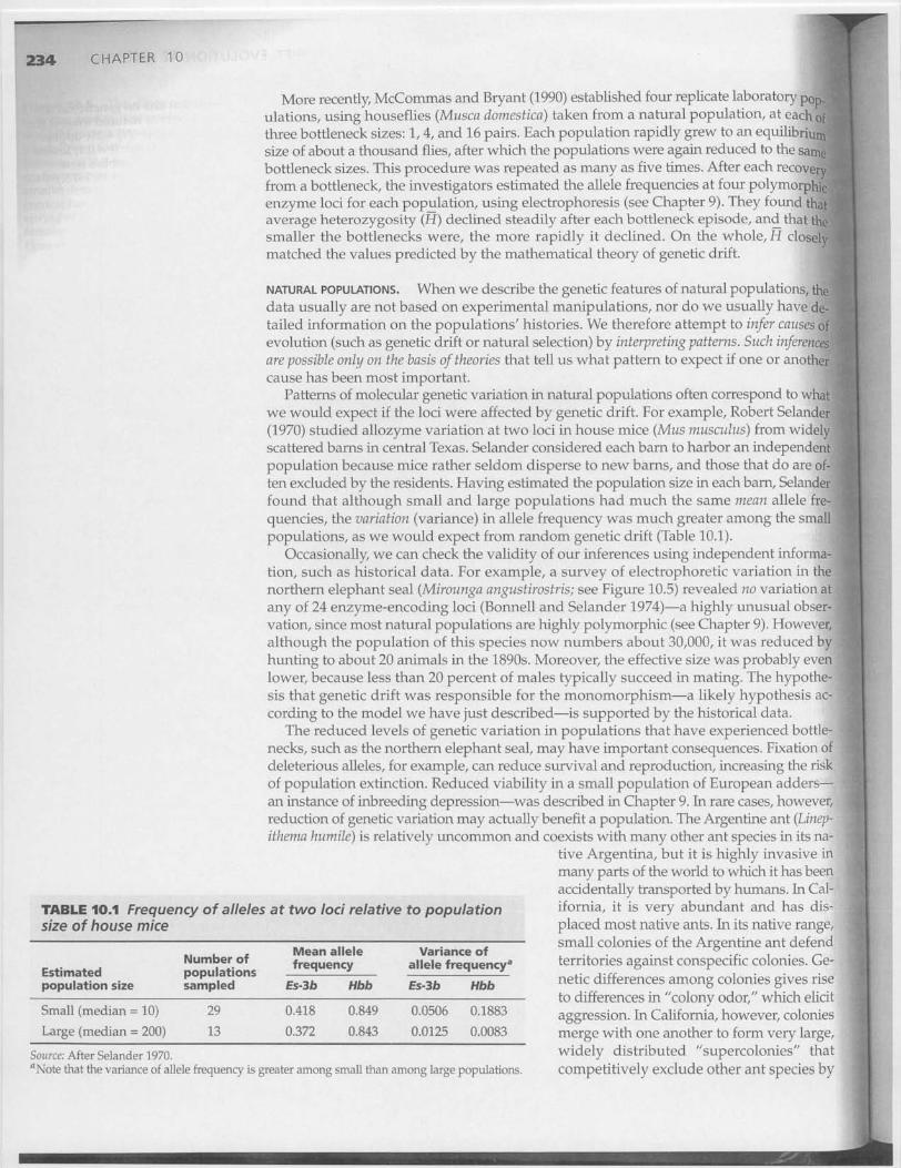
TABLE 10.1 Frequency of alleles at two loci relative to populationsize of house mice

Small (median = 10) 29

0.418 0.849

0.0506 0.1883

Large (median = 200) 13

0.372 0.843

0.0125 0.0083

Estimatedpopulation size

Number ofpopulationssampled Es-3b Hbb

Variance ofallele frequency'

Es-3b Hbb

Mean allelefrequency

Source: After Selander 1970.'Note that the variance of allele frequency is greater among small than among large populations.

More recently, McCommas and Bryant (1990) established four replicate laboratory po

ulations, using houseflies (Musca domestica) taken from a natural population, at each

three bottleneck sizes: 1, 4, and 16 pairs. Each population rapidly grew to an equilibrisize of about a thousand flies, after which the populations were again reduced to the sbottleneck sizes. This procedure was repeated as many as five times. After each recoveryfrom a bottleneck, the investigators estimated the allele frequencies at four polymorplenzyme loci for each population, using electrophoresis (see Chapter 9). They found tiaverage heterozygosity (H) declined steadily after each bottleneck episode, and that t,smaller the bottlenecks were, the more rapidly it declined. On the whole, H closelymatched the values predicted by the mathematical theory of genetic drift.

NATURAL POPULATIONS. When we describe the genetic features of natural populations, thedata usually are not based on experimental manipulations, nor do we usually have de-tailed information on the populations' histories. We therefore attempt to infer causes ofevolution (such as genetic drift or natural selection) by interpreting patterns. Such inferencesare possible only on the basis of theories that tell us what pattern to expect if one or anothercause has been most important.

Patterns of molecular genetic variation in natural populations often correspond to what

we would expect if the loci were affected by genetic drift. For example, Robert Selander(1970) studied allozyme variation at two loci in house mice (Mus musculus) from widelyscattered barns in central Texas. Selander considered each barn to harbor an independentpopulation because mice rather seldom disperse to new barns, and those that do are of-ten excluded by the residents. Having estimated the population size in each barn, Selanderfound that although small and large populations had much the same mean allele fre-quencies, the variation (variance) in allele frequency was much greater among the smallpopulations, as we would expect from random genetic drift (Table 10.1).

Occasionally, we can check the validity of our inferences using independent informa-tion, such as historical data. For example, a survey of electrophoretic variation in thenorthern elephant seal (Mirounga angustirostris; see Figure 10.5) revealed no variation atany of 24 enzyme-encoding loci (Bonnell and Selander 1974)—a highly unusual obser-vation, since most natural populations are highly polymorphic (see Chapter 9). However,although the population of this species now numbers about 30,000, it was reduced byhunting to about 20 animals in the 1890s. Moreover, the effective size was probably evenlower, because less than 20 percent of males typically succeed in mating. The hypothe-sis that genetic drift was responsible for the monomorphism—a likely hypothesis ac-cording to the model we have just described—is supported by the historical data.

The reduced levels of genetic variation in populations that have experienced bottle-necks, such as the northern elephant seal, may have important consequences. Fixation ofdeleterious alleles, for example, can reduce survival and reproduction, increasing the riskof population extinction. Reduced viability in a small population of European adders—an instance of inbreeding depression—was described in Chapter 9. In rare cases, however,reduction of genetic variation may actually benefit a population. The Argentine ant (Linep-ithema humile) is relatively uncommon and coexists with many other ant species in its na-

tive Argentina, but it is highly invasive inmany parts of the world to which it has beenaccidentally transported by humans. In Cal-ifornia, it is very abundant and has dis-placed most native ants. In its native range,small colonies of the Argentine ant defendterritories against conspecific colonies. Ge-

netic differences among colonies gives riseto differences in "colony odor," which elicitaggression. In California, however, coloniesmerge with one another to form very large,widely distributed "supercolonies" thatcompetitively exclude other ant species by

GENETIC DRIFT: EVOLUTION AT RANDOM 235

(A) Intraspecific aggression

High

4—

3

• • •

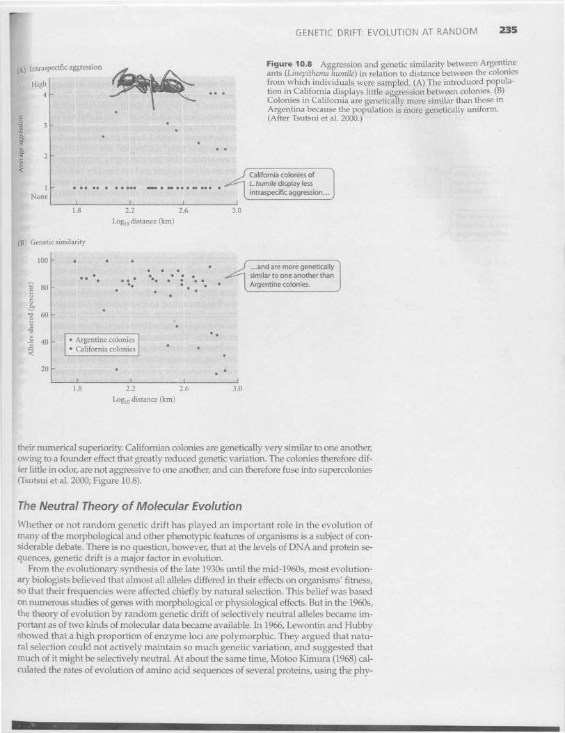
Figure 10.8 Aggression and genetic similarity between Argentineants (Linepithema humile) in relation to distance between the coloniesfrom which individuals were sampled. (A) The introduced popula-tion in California displays little aggression between colonies. (B)Colonies in California are genetically more similar than those inArgentina because the population is more genetically uniform.(After Tsutsui et al. 2000.)

• •

V▪2

California colonies of

• • • • • • • • • •• •••• •• •MI • • •• ••• ••• • •• L. humile display less

intraspecific aggression... j

1.8

2.2 2.6 3.0

Log io distance (km)

(B) Genetic similarity

1None

100 • ...and are more geneticallysimilar to one another thanArgentine colonies.C 80

VUVV

• 60

aro

40

• • •

• •• •• • •

• • •• •• •• •• •••• • •

• ••

• Argentine colonies

• California colonies

20 • ••

1.8

2.2 2.6

3.0

Logi o distance (km)

their numerical superiority. Californian colonies are genetically very similar to one another,owing to a founder effect that greatly reduced genetic variation. The colonies therefore dif-fer little in odor, are not aggressive to one another, and can therefore fuse into supercolonies(Tsutsui et al. 2000; Figure 10.8).

The Neutral Theory of Molecular EvolutionWhether or not random genetic drift has played an important role in the evolution ofmany of the morphological and other phenotypic features of organisms is a subject of con-siderable debate. There is no question, however, that at the levels of DNA and protein se-quences, genetic drift is a major factor in evolution.

From the evolutionary synthesis of the late 1930s until the mid-1960s, most evolution-ary biologists believed that almost all alleles differed in their effects on organisms' fitness,so that their frequencies were affected chiefly by natural selection. This belief was basedon numerous studies of genes with morphological or physiological effects. But in the 1960s,the theory of evolution by random genetic drift of selectively neutral alleles became im-portant as of two kinds of molecular data became available. In 1966, Lewontin and Hubbyshowed that a high proportion of enzyme loci are polymorphic. They argued that natu-ral selection could not actively maintain so much genetic variation, and suggested thatmuch of it might be selectively neutral. At about the same time, Motoo Kimura (1968) cal-culated the rates of evolution of amino acid sequences of several proteins, using the phy-