&lufohdqg 6txduh - oit.ac.jp › center › ~nakanishi › english › seta2019...2019/06/02...

$: &LUFOHDQG 6TXDUH - oit.ac.jp › center › ~nakanishi › english › SETA2019...2019/06/02 · 6(7$ 6KLQJR 1DNDQLVKL 2VDND ,QVWLWXWH RI 7HFKQRORJ\ -$3$1 H 7R\RQDND&DPSXV # 2VDND$
SETA2019 （Toyonaka Campus @ Osaka Univ.） June 2nd, 2019 © Shingo Nakanishi (Osaka Institute of Technology, JAPAN)

Symmetric Relations and Geometric Characterizations about Standard Normal Distributionby Circle and Square

1

Pearson’s finding probability point:

Its cumulative distribution probability:

Kelley’s formulation as 27 percent rule:

Standard Normal Distribution

(Aspect Ratio: ,)

Please remember the following values.

Eva

luat

ions

Random Walking

Shingo NAKANISHI (Osaka Inst. of Tech., Japan)Masamitsu OHNISHI (Osaka Univ., Japan)

𝟎. 𝟔𝟏𝟐𝟎𝟎𝟑

−𝟎. 𝟔𝟏𝟐𝟎𝟎𝟑

Grouping such as the proposal by Cox

Good

Bad

Middle

© Shingo Nakanishi (Osaka Institute of Technology, JAPAN)SETA2019 （Toyonaka Campus @ Osaka Univ.） June 2nd, 2019

2

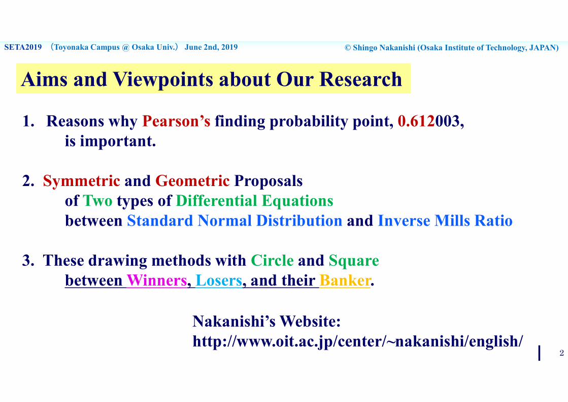
1. Reasons why Pearson’s finding probability point, 0.612003, is important.

2. Symmetric and Geometric Proposals of Two types of Differential Equationsbetween Standard Normal Distribution and Inverse Mills Ratio

3. These drawing methods with Circle and Squarebetween Winners, Losers, and their Banker.

Aims and Viewpoints about Our Research

Nakanishi’s Website:http://www.oit.ac.jp/center/~nakanishi/english/


𝑋𝛼

,𝑡

3

Changing the fee under the condition

Number of trial: 𝑡

0

𝐸(𝑌

𝛼,𝑡

)

The fee is equal to （） times ofbased on Ref. TORSJ，55,1-26（2012）

Winners Maximal Profit are equilibrium to its Fee by a Banker at t=1 and s=1

Profit of a Winner :𝑌 𝛼, 𝑡 = max(𝑋 𝛼, 𝑡 , 0)

Loss of a Loser :𝑌 𝛼, 𝑡 = min(𝑋 𝛼, 𝑡 , 0)

Number of trial: 𝑡

Dashed curve is a winner’s expected profit which is greater than 0 :

The maximal profit for winners is a parabolabased on the winners probability 0.2702678constantly.

Equilibrium formulation :

If and ,

Integral from 0 to ∞ of PDF


4

𝑈 𝑡 = 𝜆Φ −𝜆 𝑡

𝑈 𝑡 = 𝜆(1 + Φ −𝜆 ) 𝑡

𝑉 𝑡 = 𝜆Φ −𝜆

Φ −𝜆𝑡 = 𝜆 𝑡

𝑉 𝑡 = 𝜆1 + Φ −𝜆

1 − Φ −𝜆𝑡 𝛼𝑡

𝜆 𝑡

(Aspect Ratio:𝟏. 𝟎)

Ref. TORSJ，55,1-26（2012）

Ref. ORSJ(@Kansai Univ. in Sep., 2017)

Risk Aversion

Risk Preference


5

Relations between Inverse Mills Ratio, Conditional Expectation, and

1

2𝜋

2

2𝜋

u*=0.30263084

𝑔 𝑢 =𝜙 𝑢

Φ 𝑢


Φ −𝑢

Bernoulli differential equations

Ref. RIMS2078-10（@Kyoto Univ. in Nov., 2017）Ref. ORSJ（@Keio Univ. in Mar., 2016）

Kelley’s 27 percent rule, , shows

the conditional expected values:


6

Inverse Mills Ratio, Standard Normal Distribution, and Bernoulli Differential Equations

Ref. RIMS2078-10（Kyoto Univ. in Nov., 2017）

Kelley’s 27 percent rule,


−1

𝜆𝑢 +

1

𝜆Φ −𝜆𝑣 = 1

−1

𝜆𝑢 +

1

𝜆𝑣 = 1

−1

𝜆1 + Φ −𝜆1 − Φ −𝜆

𝑢 +1

𝜆 1 + Φ −𝜆𝑣 = 1

: Entire Viewpoint（Vertical axis）: Individual Viewpoint（Horizontal axis）

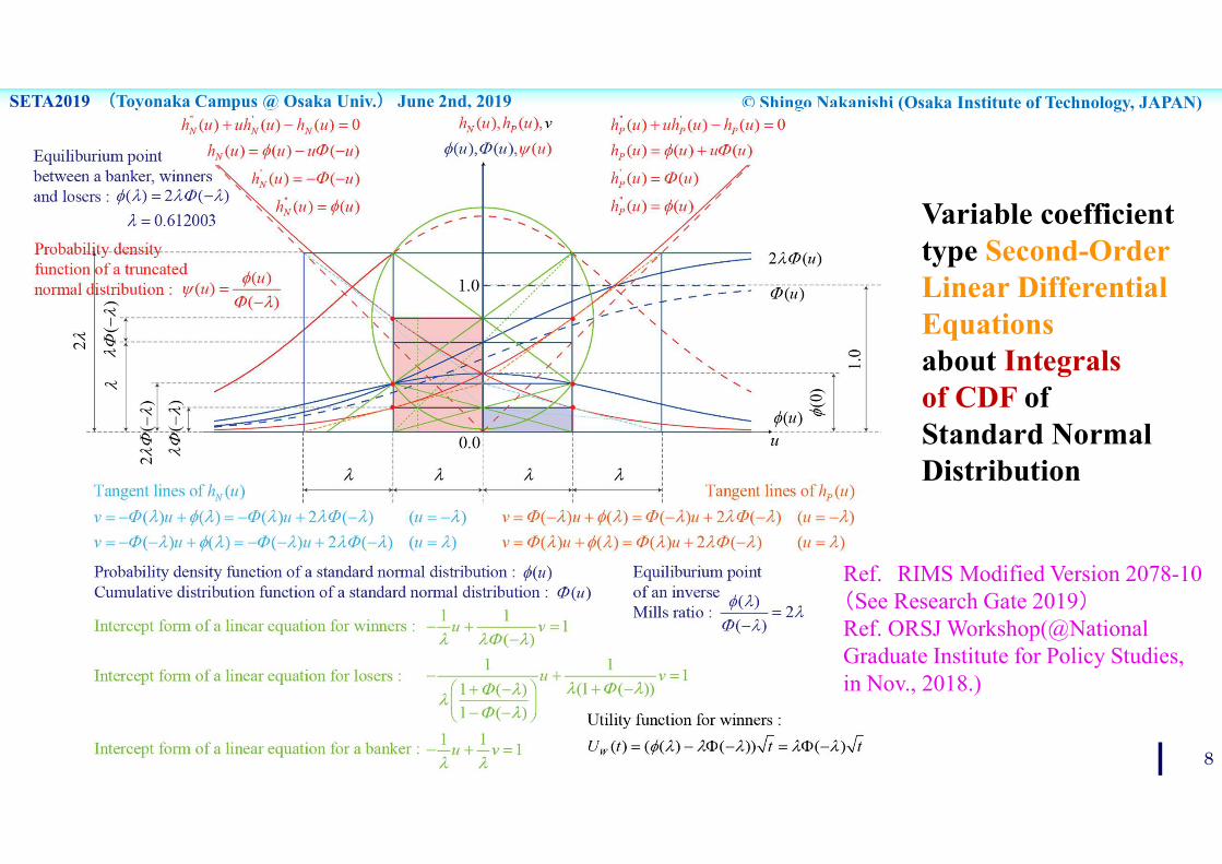
Intercept form of a linear equation for winners :

Ref. ORSJ（@Kansai Univ. in Sep., 2017）

Intercept form of a linear equation for losers :

Intercept form of a linear equation for their banker :

Standard Normal Distributionby Circle and Squarefor Winners, Losers, and their Banker


8

Ref. RIMS Modified Version 2078-10（See Research Gate 2019）Ref. ORSJ Workshop(@National Graduate Institute for Policy Studies,in Nov., 2018.)

Variable coefficient type Second-Order Linear Differential Equationsabout Integrals of CDF of Standard Normal Distribution


9

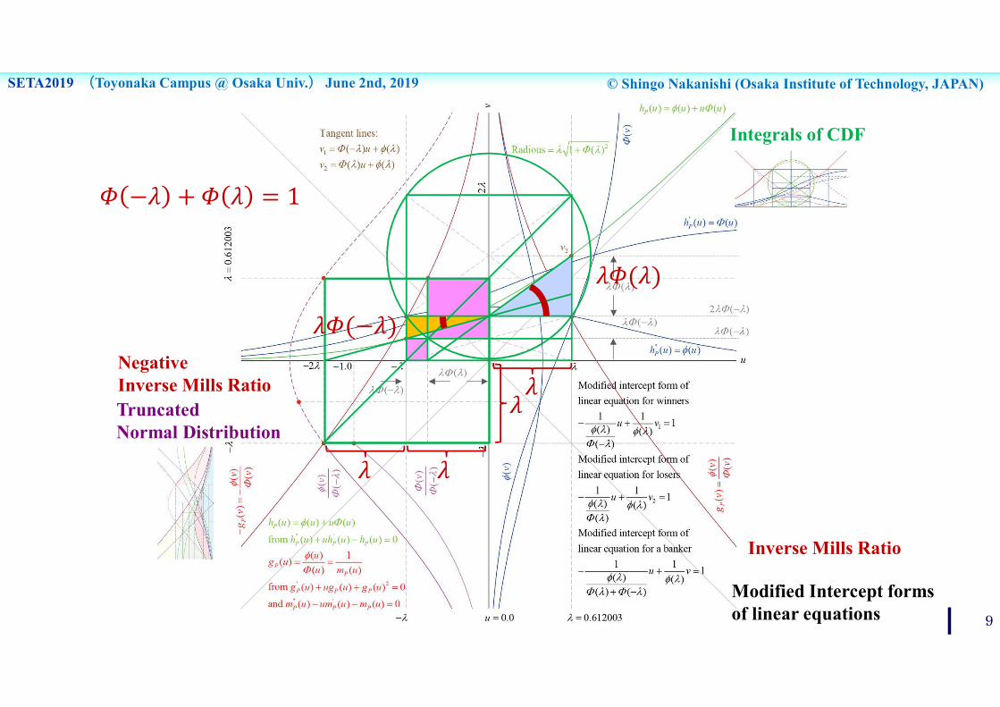
Integrals of CDF

Inverse Mills Ratio

Negative Inverse Mills RatioTruncatedNormal Distribution

Modified Intercept formsof linear equations


10

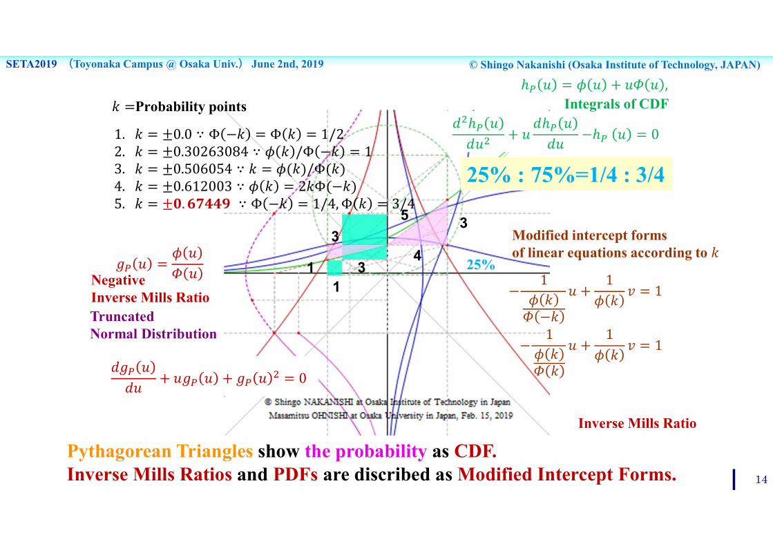
1. 𝑘 = ±0.02. 𝑘 = ±0.302630843. 𝑘 = ±0.5060544. 𝑘 = ±0.612003(= 𝜆)5. 𝑘 = ±0.67449

−1

𝜙 𝑘𝛷 −𝑘

𝑢 +1

𝜙 𝑘𝑣 = 1

−1

𝜙 𝑘𝛷 𝑘

𝑢 +1

𝜙 𝑘𝑣 = 1

Modified intercept forms of linear equations according to 𝑘

𝑢

𝑣

0

𝑘 =Probability points Integrals of CDF

Inverse Mills Ratio



11

1. 𝑘 = ±0.02. 𝑘 = ±0.302630843. 𝑘 = ±0.5060544. 𝑘 = ±0.612003(= 𝜆)5. 𝑘 = ±0.67449

−1


𝑢 +1

𝜙 𝑘𝑣 = 1

−1

𝜙 𝑘𝛷 𝑘

𝑢 +1

𝜙 𝑘𝑣 = 1

𝑢

𝑣

0



Inverse Mills Ratio



12

1. 𝑘 = ±0.02. 𝑘 = ±0.302630843. 𝑘 = ±0.5060544. 𝑘 = ±0.612003(= 𝜆)5. 𝑘 = ±0.67449

−1


𝑢 +1

𝜙 𝑘𝑣 = 1

−1

𝜙 𝑘𝛷 𝑘

𝑢 +1

𝜙 𝑘𝑣 = 1

𝑢

𝑣

0



Inverse Mills Ratio


The proportion :


13

1. 𝑘 = ±0.02. 𝑘 = ±0.302630843. 𝑘 = ±0.5060544. 𝑘 = ±0.612003(= 𝜆)5. 𝑘 = ±0.67449

−1


𝑢 +1

𝜙 𝑘𝑣 = 1

−1

𝜙 𝑘𝛷 𝑘

𝑢 +1

𝜙 𝑘𝑣 = 1

𝑢

𝑣

0



Inverse Mills Ratio



14

1. 𝑘 = ±0.0 ∵ Φ −𝑘 = Φ 𝑘 = 1/22. 𝑘 = ±0.30263084 ∵ 𝜙 𝑘 /Φ −𝑘 = 13. 𝑘 = ±0.506054 ∵ 𝑘 = 𝜙(𝑘)/Φ(𝑘)4. 𝑘 = ±0.612003 ∵ 𝜙 𝑘 = 2𝑘Φ(−𝑘)5. 𝑘 = ±𝟎. 𝟔𝟕𝟒𝟒𝟗 ∵ Φ −𝑘 = 1/4, Φ 𝑘 = 3/4

3

311

34

5

25%

25% : 75%=1/4 : 3/4

−1


𝑢 +1

𝜙 𝑘𝑣 = 1

−1

𝜙 𝑘𝛷 𝑘

𝑢 +1

𝜙 𝑘𝑣 = 1

Pythagorean Triangles show the probability as CDF.Inverse Mills Ratios and PDFs are discribed as Modified Intercept Forms.

ℎ 𝑢 = 𝜙 𝑢 + 𝑢𝛷 𝑢 ,


𝛷 𝑢

𝑑𝑔 𝑢

𝑑𝑢+ 𝑢𝑔 𝑢 + 𝑔 𝑢 = 0

𝑑 ℎ 𝑢

𝑑𝑢+ 𝑢

𝑑ℎ 𝑢

𝑑𝑢−ℎ 𝑢 = 0



Inverse Mills Ratio



15

Concluding Remarks1. Importance of

Pearson’s finding probability point, 0.612003.2. Symmetric Relations and Geometric Characterizations

about Two types of Differential Equationsbetween Standard Normal Distribution and Inverse Mills Ratio.

3. Greek Pythagorean Theorem about CDFand Ancient Egyptian Drawing Styles with Circle and Square.

4. Proposals of Modified Intercept Formsfor Winners, Losers, and Their Banker.

AcknowledgmentsWe would like to express our sincerely gratitude to Prof. Kosuke OYA and Prof. Hisashi TANIZAKI belonging to the Graduate School of Economics at Osaka University. The first author, Shingo NAKANISHI, would like to show my grateful to Prof. Hidemasa YOSHIMURA, Associate Prof. Manami SATO, Prof. Tsuneo ISHIKAWA and Prof. Yukimasa MIYAGISHI belonging to Osaka Institute of Technology. And the first author would particularly like to thank Prof. Takeshi KOIDE at Konan University, Associate Prof. Hitoshi HOHJO at Osaka Prefecture University, Prof. Shoji KASAHARA at Nara Institute of Science and Technology, Prof. Jun KINIWA at University of Hyogo. Especially, we would like to show full of our appreciations to Prof. Tetsuya TAKINE belonging to the Graduate school of Engineering at Osaka University, Prof. Hiroaki SANDOH at Kwansei Gakuin University and many other members at Operations Research Society of Japan (ORSJ) and Kansai-tiku Koryukai at the Securities Analysts Association of Japan (SAAJ).

Thank you for your kind attention.

&lufohdqg 6txduh - oit.ac.jp › center › ~nakanishi › english › seta2019...2019/06/02...

Documents