MAESTRÍA EN ECONOMÍA

TRABAJO DE INVESTIGACIÓN PARA OBTENER EL GRADO DE MAESTRO EN ECONOMÍA

THE DETERMINANTS OF PROFITABILITY IN THE BANKING SECTOR: EVIDENCE FROM MEXICO

JOSÉ MIGUEL LARRIETA ARTEAGA

PROMOCIÓN 2018-2020

ASESOR:

ENEAS ARTURO CALDIÑO GARCÍA

SEPTIEMBRE 2020

«This page is intentionally left blank.»

To my family

i

Acknowledgement

I wish to show my gratitude to:

My family whose unquestioning and selfless support were the basis of my presentself.

To my advisor and professor Dr. Eneas Arturo Caldiño García, who taught me,advised me and supported me before, during and after the fulfillment of this document.

Dr. Omar Augusto Guerrero García, for his invaluable mentoring and unconditionaltutoring, whose teachings were an absolute necessity for the completion of this work.

Dr. José Jorge Mora Rivera for his noble and sincere counseling and guidance.

My classmates and friends for their intellectual challenges, keen advices and theirundoubted friendship and support.

All my professors from El Colegio de México for their valuable education and sharedknowledge.

ii

Abstract

The present study aims at analyzing the most relevant factors, thus, determinantsthat impact the profitability of banks in Mexico. Using the financial statements of thebanks in Mexico, three panel data sets were constructed to evaluate the most relevantvariables employing a fixed effects model for two periods, namely 2007-2019 and 2001-2019. Analyzing internal components, industry specific and macroeconomic elements, thisstudy found that the most relevant, consistent and statistically significant explanatoryvariables for profits (measured by ROAA and ROAE) were liquidity, credit risk, costs andthe Mexican Stock Market Index; in contrast, macroeconomic variables did not seem tohave large effects across all types of banks, just bigger ones appear to be mostly affectedby them.

iii

Contents

1 Introduction 1

2 Variables 32.1 Internal Variables . . . . . . . . . . . . . . . . . . . . . . . . . . . . . . . 42.2 External Variables . . . . . . . . . . . . . . . . . . . . . . . . . . . . . . 8

3 Literature Review 11

4 Data 154.1 Data Treatment . . . . . . . . . . . . . . . . . . . . . . . . . . . . . . . . 15

5 Descriptive Statistics 175.1 Correlation Matrix . . . . . . . . . . . . . . . . . . . . . . . . . . . . . . 19

6 Econometric Model 24

7 Results 297.1 Before (2001-2006), During (2007-2009) and After (2010-2019) the

Financial Crisis Econometric Results . . . . . . . . . . . . . . . . . . . . 42

8 Conclusions 50

Bibliography 53

Appendix 56

List of Tables 88

iv

Chapter 1

Introduction

Banks are central agents in any economy, and having a sound banking sector iscrucial to financial and economic stability in a country. They are an effective channel inthe creation of new businesses, they provide assistance for the growth of firms throughloans, the central bank relies intensively on them for economic acceleration, theyprovide financial security to agents, among many other attributes (Menicucci andPaolucci, 2016; Chavarín, 2016). The importance and centrality of banks isindisputable; therefore, having a healthy banking sector increases the possibility ofgrowth and stability. Furthermore, their poor management, could have potential majordisruptions in the economy. Using econometric techniques with panel data for mainlytwo periods, namely 2001-2019 and 2007-2019, internal components, industry specificand macroeconomic elements, the present work aims at analyzing the main aspects,thus, determinants, that influence the banks’ profits, measured by Return on AverageAssets and Return on Average Equity, in Mexico.

The present study has three main contributions. First, it enlarges the currentliterature on determinants of banks’ profitability in Mexico, which in general, has beenlimited. It is important to have an overview of the banking sector from differentperspectives since they are crucial agents in the financial system and their managementis relevant for the economy. Second, most of the reviewed studies used industry specificvariables such as market power or market share, but very few considered the stockmarket as an explanatory variable. This study incorporates the Mexican Stock MarketIndex (IPC) because it hypothesizes that as banks grow larger, their network does aswell, meaning that their relation with larger firms will most likely grow; in this sense,changes in the market captured by the stock market index, may influence the banks

1

profits as well. In Mexico, the index is calculated considering a sample of 35 firms fromdifferent sectors that operate in the country; therefore, we would expect that if there isa reward from the market towards these companies, then, the banks profits couldbenefit as well, we believe this to be specially true for larger banks. Third, it encouragesscholars to examine this particular research question in order to provide additionalevidence about the factors influencing the banks profits, specially for Mexico.

The document is arranged in the following way. Section 2 describes in detail thevariables used, why were they employed and how did other authors utilize them. Section3 briefly examines the literature that have scrutinized in the determinants of banks’profits around the world. Section 4 discusses the data used and its treatment for thefinal data bases. Section 5 addresses the descriptive statistics and correlations from theinformation. Section 6 uncovers the econometric model. Section 7 present the findingsof the present work and compare the results with the previous studies. Finally, Section8 concludes.

2

Chapter 2

Variables

In the determinants of banks’ profitability literature, the question is adressed withbasically three types of variables. The first type are internal variables, in which equity,assets, costs, management, credits, risks, among others are considered. The second typeare market associated variables. In general, the market power measured by theHerfindahl-Hirschman Index and the market share calculated by the particular banks’assets relative to total industry assets, are the most common variables to assess themarket effects on profits. Nonetheless, in the present work IPC (the Mexican StockMarket Index) is also incorporated as an independent variable which may, arguably,have some market effects in banks’ profitability. The third type are macroeconomicvariables; these are often used because they are independent of the decisions of themanagers, and all banks are exposed to them. The most commonly used variables areeconomic growth and inflation.

Most independent variables, particularly the internal variables, with the exception ofsize, are measured with ratios. As Menicucci Paolucci (2015) establish, ratios are usedbecause they are inflation-invariant. They also state that the numerator anddenominator in ratios are measured in monetary terms, therefore profits could actuallycapture the real effects from the inflation rates which vary over time.

3

2.1 Internal Variables

ROE/ROAE (Return on Equity/Return on Average Equity) - This is one of the mostused variables in the literature to measure profits. It is a ratio of the net return and theshareholders’ capital or equity, this is also an indicator for profits since it compares howmuch is the net return of the bank relative to what has been offered by shareholders, inother words, it measure their returns relative to the value of what they invested.Compared to the Return on Assets (ROA) indicator, ROE is a much more variable.This is due to the fact that total assets are more complicated to vary than equity. Oneof the drawbacks of this measurement is that it ignores the higher risk that is associatedto high leverage and the effect that regulation has on it (Medeiros and Martins, 2016).Particularly for this work, the average was used, meaning that the Return on AverageEquity indicator was utilized as a dependent variable.

ROA/ROAA (Return on Assets/Return on Average Assets) - In the literature ofdeterminants of banks profitability, Return on Average Assets is the other most usedvariable to approximate the profitability of a Bank. It is basically a ratio of the netreturn to total assets. Specifically for the analysis, the yearly averages were used in thisstudy (ROAA). Menicucci and Paolucci (2016), Li (2007) also state that ROA can beconsidered to compare operating performance of banks, which may be an importantfactor when analyzing banks’ profits. ROA also indicate how the funds and assets arebeing managed to generate revenues (Menicucci and Paolucci, 2016; Dietrich andWanzenried, 2014). It is also argued that banks usually report a lower ROE due to alower leverage ratio, in which having another measurement for profits, such as ROA, isuseful.

Profits indicators are measured in ratios, this allow us to observe the relativemovement in variables, rather than looking at the absolute terms. In this way, theheterogeneity within the data, namely, information of large and small banks, could beuseful to measure profits. It could be argued that since small banks face less operativecosts, they could have, relatively, larger profits than bigger banks. Moreover, sincevariables could act different on profits we included the two indicators of profits, namelyROAA and ROAE, in order to have additional certainty about the results.Furthermore, each one may capture effects not considered by the other, as Petria et. al.(2015) state, a possible drawback or ROA is the existence of the off-balance sheet assets

4

are not considered in this measurement, in which ROE is more accurate (Goddard et.al., 2004 in Petria et. al., 2015). It is important to consider that we chose ROAA andROAE over ROA and ROE for mainly two reasons. The first has to do with the factthat when we use the average, meaning, ROAA and ROAE the transactions over thewhole year are captured specially during the fiscal year, this could also possibly assessthe fact that decisions in one month do not only impact that particular one, but futureperiods as well; second, since the previous study used the average as well, we wanted tohave the same variable for comparison. As Dietrich and Wanzenried (2014) state theaverage captures asset movements on a fiscal year.

Size - The natural logarithm of the total assets variable was used. As Dietrich andWanzenried (2014) point out, measuring size with the total assets could not be ideal,specially for the largest banks, which have high off-balance sheet activities.Nonetheless, a uniform measure of bank size is needed and this is an standard anduseful way to do it. Al-Harbi (2019) and Li (2007) state that size is introduced as a wayto account for economies or diseconomies of scale, where the former have positive effectsand the latter have negative impact. Using this definition, it is a fact that bigger bankshave larger amounts of total assets, but arguing that they have a purely positive impacton banks’ profits is not obvious. There is evidence that using this measurement of size,effects on profits could go both sides, positive or negative. Petria et. al. (2015), Öhmanand Yazdanfar (2018), Dietrich and Wanzenrie (2014) argue that increasing size couldgenerate economies of scale, and thus, performance. Menicucci and Paolucci (2016) saythat larger banks could also be benefited from economies of scope, with reduced risksand product diversification, and argue too that this could potentially lead larger banksto enter into markets where small banks can’t. In contrast, profits could also benegatively affected given that larger banks could possibly be affected more bybureaucracy, rigidities and inefficiencies (Öhman and Yazdanfar, 2018; Dietrich andWanzenried, 2014).

Capital Asset Ratio - This variable is included to test a possible effect fromcapitalization on profits. The variable is constructed as the ratio between equity andthe total assets. It is used to observe how much capital lies behind the bank, is a way tomeasure the strength or adequacy of the capital. Li (2007) argues that capital strengthcould have a positive effect on profits because the higher the ratio, the less necessitythere is of external funding, thus, higher profits. It is also asserted that well capitalized

5

banks are less risky; more secure in the sense that they are more resistant againstfinancial crisis and may be able to provide security for depositors; they are alsoconsidered to be less likely to go bankrupt; and it is argued that a bank with morecapital strength has access to funding at a lower cost, increasing profits (Al-Harbi, 2019;Menicucci and Paolucci, 2016; Medeiros and Martins, 2016; Li, 2007). On contrast, anexceedingly elevated level of capitalization could possibly mean that banks’ operationsare highly cautious could ignore investment opportunities; moreover, in line with therisk-return hypothesis, there is an inverse relation between capitalization and profits,since they tend to borrow less and have lower risk, returns could be lower too. (Öhmanand Yazdanfar, 2018, Ghosh, 2016). Effects of capital adequacy on profits are not selfevident, thus results could indicate a positive or negative impact.

Deposit Asset Ratio - It is a ratio that gives information about how much moneythe bank owes (to depositors) in relation to the amount of assets possessed by the bank.As Menicucci and Paolucci (2016) assert, banks rely substantially on deposits toallocate credits. Banking sector, specially commercial banks, try to find clients in needof credit, get profits on interests and are committed to have sufficient funds for thosecustomers who wish to withdraw money. Therefore, imposing a constraint on demandsfor loans, must have an impact on the opportunity cost of deposits. Al-Harbi (2019)argues that since deposits represent a primary source of funds at a low cost, itsenlargement could positively affect profits on the basis that demand for loans continues.The author also states, in the same way as Menicucci and Paolucci (2016) do, that thelack of loan demand are causes for deposits to become costlier in terms of funds, andthat reduces profits. If people stop demanding loans, opportunity cost of moneyincreases, and that makes every monetary unit to be more expensive given that optionsfor releasing it diminish. Dietrich and Wanzenried (2014), argue that a higher growthrate of deposits may help in the business expansion and this could lead to greaterprofits; nonetheless, it is also stated that this is not necessary since the bank need to beable to transform those deposits into actual additional income. Finally, we could seethat deposits represent a cost for the bank since more deposits mean more operatingcosts, Medeiros and Martins (2016) argue that management has to be very efficient totransform those deposits into future profits. In this sense the deposit asset ratio couldgo in both directions.

Loan Asset Ratio - There are mainly two elements used to construct a total loan

6

variable, namely, outstanding loan and the due loan portfolios. These variables indicatehow much has the bank lend to agents and how much it is owed by them. Outstandingloan measures the credits that have been payed, and due loan are the loans that remainunpaid by the agent. Both are considered assuming that due loans will be paid and thebank, and eventually, it will be able to use them. As banks receive interests for all loansthey offer, it is expected that profits could be higher as loans go higher. However,literature is not conclusive about a positive effect, there are some possible causes thatmay offer an explanation for a negative relationship. As banks grow, their loan supplydoes as well, this could also mean an increase in costs (Al-Harbi, 2019). Other reasonscould be that a higher growth in volume of loans could affect credit quality;additionally, if the increase in loans is due to lower margins, then profits could bediminished (Menicucci and Paolucci, 2016).

Loan Deposit Ratio - This is an indicator for liquidity, it is constructed as a ratioof the total loan and the deposits. It gives information about how much income thebank is receiving from credits and how much it owes in deposits. It could be seen as anindicator for the freedom that the bank possess in order to make operations in themarket. Chavarín (2016) uses the same variable; however, Adelopo et. al. (2018)calculates liquidity using liquid assets divided by total customer and short-termfunding. The first was used to compare results with an study for the same country.Results on this variable are mixed but they are further explored in the results section.Adelopo et. al. (2018) and Ahokpossi (2013) use these variable, plus short-term fundingas a proxy for credit risk, arguing that the higher is the value of the ratio, the higherthe exposure of the bank to default risk.

Credit risk - It was measured with the preventive estimation of credit risk, whichbasically measures the proportion of the credit that won’t have a viability for payment,over total loans. Medeiros and Martins (2016) assert that when credit risk is highercredit quality decreases, which lead to lower profitability. Adelopo et. al. (2018) pointsout that banks may be able to encounter credit risk by two means. The first is beingtheir exposure to significant default rates on loans; the second, is due to inadequatereserves or insolvency. Ahokpossi (2013), as mentioned before, used loans to depositsand short term funding as a proxy for credit risk, finding a positive relationship withprofits (using net interest margin). Dietrich and Wanzenried (2014) mention thattheory supports the idea that an increased exposure to credit risk is more likely to be

7

related to a decrease in profits. Most studies using credit risk as a determinant appearto have enough reasons to believe that it is negatively associated to banks’ benefits.

Costs - This variable measures the administrative cost relative to total assets. Thereis no actual debate on whether the costs offer a positive or negative impact, evidence isclear that they decrease the level of profitability in bank; rather the degree to which theyaffect profits is addressed.

2.2 External Variables

Market Share - This variable was measured by the banks assets relative to the totalamount of existing assets in the period. It is possible to argue that if a bank has alarger share of the market, then it could have more profits. The variable wasconstructed using the relationship of every bank to a common variable thatencompassed all banks which is Total Banca Multiple which basically has theaggregated information for all the banks in all the periods. Since this information iscalculated for all years, independently if a new bank appears, or one disappears, it waseasier to make it the benchmark. The total assets of every bank was compared directlyto the aggregated, this eliminates the issue that arises when the quantity of bankschanges over time (mergers, bankruptcy, etc.). It is important to note that addressingmarket concentration or market power in the banking sector is not the main scope ofthis work, further analysis is needed in order to address the question of whether thebaking sector is concentrated and efficient or not.

IPC - This is the Mexican Stock Market Index, it is calculated considering a pool offirms operating in the economy and it provides information about the financialenvironment of the country since it reflects the evolution of the stock market. Giventhat banks trade an enormous amount of money in the economy, it is natural to thinkthat stock markets which are directly related to big companies, could possibly have aneffect in the banks’ profits. Notwithstanding, most studies explored in the literaturereview on determinants of banks’ profits did not use an stock market index as anexternal variable. The IPC is a direct observation of market behavior; furthermore, itcould be seen as a measure of confidence. It is expected that as banks grow larger, theirnetwork does as well, meaning that they are most likely to have interactions with biggerfirms. In this sense, it is hypothesized that if companies are rewarded by the market,

8

this will have a positive impact on banks’ profits, specially for larger banks. Monthlydata was obtained from the public information of the Central Bank, specifically, thegrowth rate of the index was used as an explanatory variable of profits. Dietrich andWanzenried (2014) included the value of shares relative to the GDP as an indicator ofthe degree of financial market development.

Inflation - The inflation rate was used, measured with the National ConsumerPrice Index annual growth. As Dietrich and Wanzenried (2014) point out, the effectthat inflation has on bank profits, depends on the growth rate of wages and operatingexpenses in relation to inflation. They also stated that if banks do not anticipateinflation and do not adjust their interest rates, then costs may increase faster andprofits could be reduced. Additionally, Ahokpossi (2013) claims that inflation alsomight be seen as a risk given that it could affect margins; this is the case if lending anddeposit rates adjust in different speed and extent to the monetary shocks presented inthe economy. Adelopo et. al. (2018) argue that inflation affects costs, thus reducingprofits. However, inflation could increase firms’ incentives to produce more, since theycould potentially make more profits, consequently this could positively affect banks’benefits through loans.

IGAE - This is the Global Indicator for Economic Activity which is used to get ourindicator for economic growth. Our data has a monthly periodicity, and therefore usingGDP would not be as accurate since it is constructed quarterly. In order to havemonthly information we would have to impute the rest of the data, and it will mostlikely have impacts on dispersion and variance. This indicator includes Primary,Secondary and Tertiary Activities, although fishing, forest usage, corporations andother service activities are not used in its calculation. Economic growth affects allbanks, they all face the same macroeconomic conditions; however, the way situationsare addressed are different. Generally speaking, economic growth could be associatedwith higher profits, given the created opportunities in a growing economy; the fact thatas disposable income raises the demand for loans and supply of deposits will have mostlikely an increase as well; that poor economic conditions may also affect profits bygenerating credit losses; and that higher economic growth is also associated with lowerprobabilities of default and higher access to credit (Al-Harbi, 2019; Adelopo et. al.,2018; Ghosh, 2016; Medeiros and Martins, 2016; Dietrich and Wanzenried, 2014; Li,2007). Thus, it is most likely expected that economic growth rate will have a positive

9

relation with profits.

10

Chapter 3

Literature Review

The issue addressed in this work has has been exhaustively examined by academicsworldwide; nevertheless, regions such as Latin America, and specially Mexico, havebeen overlooked. The literature about determinants of banks’ profits in Mexico hasbeen scarce; out of the literature reviewed only one article regarding this specific issuewas found (there are others regarding market power or efficiency, but their scopes aredifferent). Applying a dynamic panel data regression using the first lag of theprofitability, Chavarín (2016) analyzed the determinants of commercial banks’profitability in Mexico for the period 2007-2013. He calculated the profits using Returnon Average Assets (ROAA) and Return on Average Equity (ROAE) where ROAE hadthe most robust results. He found that the first lag of the profits was positive andsignificant with a relatively high coefficient (around .40) arguing that it reflects barriersof entry and obstacles to competition. He mentions capital and income coming fromfinal balance commissions and fees as the main factors, having a positive impact onprofits, and costs with a negative effect on them.

As mentioned, the literature addressing this particular question is extensive, interms of the variables of profits most studies use Return on Assets (ROA) and Returnon Equity (ROE) as proxies, although the Net Interest Margin (NIM) is also employed.The current work uses both Return on Average Assets (ROAA) and Return on AverageEquity (ROAE) to approximate profits. Some studies have used cross-country data,while others focused on a single country analysis. Moreover, most works utilize paneldata, having a pool of banks over the course of several years, were the most commoneconometric techniques used to address the research question are, fixed effects orrandom effects models, and dynamic panel data regressions.

11

For example, Adelopo et. al. (2018) used a fixed effects model using panel data fromthe Economic Community of West African States’ bank data base from 1999 to 2013 toanalyze the determinants of profits in the periods before, during and after the financialcrisis; Menicucci & Paolucci (2016) utilized a linear regression model on panel datafrom the top 35 banks in the European banking sector during the period 2009-2013;Capraru & Ihnatov (2014) analyzed with a linear equation and robust check withdummy variables the data retrieved from 143 commercial banks in central and easternEuropean countries, for 2004-2011; Dietrich and Wanzenried (2014) used informationfrom an unbalanced data set comprising 10,165 banks in 118 countries around theglobe, encompassing high, middle and low-income countries, to examine the banksprofits with dynamic panel regressions; applying a fixed effects model to a data set of686 banks Al-Harbi (2019) investigated the effects on banks’ profits of developing andunderdeveloped countries in the Organization of Islamic Cooperation from 1989 to2008; Petria et. al. (2015) explored the impact on profits with a fixed effects modelusing yearly data of 1098 Banks from the European Union during 2004-2011:Athanasoglou et. al. (2006) looked at determinants of profits for credit institutions inthe South Eastern European region for 1998-2002, applying both fixed and randomeffects models into an unbalanced panel data set.

There are other studies, however, that focus on a single country analysis such as thisone. For example, Öhman and Yazdanfar (2018) used OLS, Fixed Effects and FeasibleGeneralized Least Squares to examine the determinants in commercial banks with asample for the period 2005-2014 in Sweden; Medeiros and Martins (2016) analyzed thecase of Portugal with a pool of 27 domestic and foreign banks and a fixed effects modelin a pre-crisis period 2002-2007 and a post-crisis period 2008-2011; Bolarinwa et. al.(2019) evaluated the banks profitability in Nigeria using a dynamic panel estimationwith the Generalized Methods of Moments, they took 15 commercial banks operating inNigeria for a panel data covering ten years, 2005-2015; Ally (2014) looks at the case of23 banks in Tanzania, comprehending large, medium and small banks for the period2009-2013, they estimated the impacts using a fixed effects model; focusing solely oncommercial banks, with a total of 69 banks, Almaqtari et. al. (2018) studied theprofitability of banks’ in India employing pooled, fixed and random effects covering2008 to 2017; with a fixed effects model, Ali and Puah (2019) examined internaldeterminants for banks in Pakistan, considering 24 commercial banks in 2007-2015;

12

regarding the period 1985-2001 and applying a linear and a dynamic regression (withthe Generalized Method of Moments) for Greek banks, Athanasoglou et. al. (2008)explored how internal and external variables affect banks’ profits.

The variables used across studies are similar, most of which are divided inbank-specific, industry-specific, and macroeconomic variables; some being moreconsistent and significant than others. In general, the variables used for profits are ROAand ROE; for internal variables, bank size, capitalization, costs and credit risk are themost common; accounting for industry specific predictors, the market power or marketshare are typically used; finally, the distinctive macroeconomic explanatory variablesare GDP growth rate and inflation rate. Of course, the specific objectives of each workrequire particular variables that are not always present in other studies.

Bank size for example, is present in most studies; however, it has been found to havemixed effects. Dietrich and Wanzenried (2014) in terms of ROAA found no evidencethat larger banks are more profitable; nonetheless, using ROAE the variable appearedto have positive effects on profits. Petria et. al. (2015) found the opposite for Europeanbanks, finding influence from size on the return on assets but not on the return onequity. Al-Harbi (2019) found no impact and Capraru and Ihnatov (2014) results showa negative and significant relation with profits, specially using return on equity; oncontrast, Adelopo et. al. (2018), Almaqtari et. al. (2018), Menicucci and Paolucci(2016), Ally (2014), Bolarinwa et. al. (2019), Ali and Puah (2019) all found, in general,a positive and significant relationship with size. Others Chavarín (2016) found itinsignificant for most cases for the dynamic model, but positive in the static one.

Something similar happens with the level of capitalization. Dietrich and Wanzenried(2014) results show that well capitalized banks tend to have higher profits when theyare measured by ROAA and using either all banks or just those from high-incomecountries; conversely, the opposite effect emerges when ROAE is used, were theyobserve that the coefficient is consistent across the levels of income of countries (low,middle or high income), being negative and significant. Adelopo et. al. (2018) arguethat the effect depends on whether a pre-crisis, crisis or post-crisis scenario isconsidered. Menicucci and Paolucci (2016), Medeiros and Martins (2016), Ally (2014)and Athanasoglou et. al. (2008) support the idea that well capitalized banks havehigher profits.

13

As expected, for the cases of costs, the evidence strongly suggest that they have anegative impact on profits. Meaning that lowering costs will lead to an increase inprofits. (Adelopo et. al., 2018; Petria et. al., 2015; Dietrich and Wanzenried, 2014;Al-Harbi, 2019; Athanasoglou et. al., 2008; Ally, 2014; Bolarinwa et. al., 2019).

Credit risk is mostly leaning towards a negative relationship with profits (Petria et.al., 2015; Dietrich and Wanzenried, 2014; Capraru & Ihnatov, 2014; Ally, 2014;Athanasoglou et. al., 2008), although there are some exceptions. Adelopo et. al. (2018)for example, found that the effect of credit risk actually depends on whether yourlooking at banks before, during or after the crisis.

The effect of macroeconomic variables is also mixed. For example, Adelopo et. al.(2018) argues that the effect that macroeconomic variables have on profits, such as GDPand inflation, depends on the analyzed period being this before, during or after thefinancial crisis; Ally (2014) argues that macroeconomic variables doesn’t seem to havean effect in banks’ profitability; Petria et. al. (2015) observe that inflation do not quiteoffer an explanation for profits movements, but GDP was found to have a positive andsignificant effect on them; Medeiros and Martins (2016) results indicate a negative andsignificant impact with GDP; Dietrich and Wanzenried (2014) results show that neitherinflation nor GDP help explaining profits changes for high-income countries, although thisresult seems to be the opposite in middle and low-income countries, where both variablesappear to be important determinants; Athanasoglou et. al. (2008) argue that the impactof inflation and cyclical output are clear; on one hand, expected inflation was found tohave a positive and significant influence; on the other, they argue that the symmetry orasymmetry of the business cycle plays an important role since it seems that the profitsare positively correlated with with the business cycle when it is above its trend. Otherstudies such as the one performed by Bolarinwa et. al. (2019) found a positive impact onprofits by both GDP growth rate and inflation, the former was positive in three dynamicmodels, but the latter only for the differenced ROA model.

14

Chapter 4

Data

The data used in the current analysis encompassed the financial statements of banks inMexico. It was obtained from the available public historical information of the NationalBanking and Securities Commission (CNBV) which is a national independent identitythat supervises and regulates banks in Mexico. The information acquired encompassedmore than 80 banks over the course of almost 19 years, namely, December 2000 untilDecember 2019. Out of the total, only about half presented sufficient information foranalysis, meaning, information for at least six years; and only about 25 banks had datafor the 19 years.

4.1 Data Treatment

Specifically, the data retrieved from the CNBV were financial statements, for each oneof the more than 80 banks operating (or that operated previously) in Mexico. Meaningthat there were more than 80 data bases which had to be integrated in a single one withthe relevant variables needed for the analysis. This is precisely what was done, the 80data bases were cleaned and ordered to be merged with one another. Additionally, someof the variables were not internal variables, but macroeconomic variables and had to beincluded in the final data base, such as Inflation, the Mexican Stock Market Index(IPC), and the Global Indicator for Economic Activity (IGAE). These variables wereobtained from the public information provided by the Central Bank and the NationalInstitute of Statistics and Geography.

The merged Data Base had, for all banks, almost 30 relevant variables that included

15

internal, macroeconomic and constructed variables (mainly the ratios described in theprevious sections). Since the panel data was unbalanced, three subsets were created outof this merged data base to make different regressions considering different banks andperiods. The first data based encompassed only the banks that had information for atleast six years, after 2006. The second comprised banks that possessed data for at least10 years after 2006. The final subset had only the banks that owned completeinformation1 for the 19 years, 2000 to 2019. It is worth mentioning that this data baseis associated with the larger banks, meaning that those that have been present since thebeginning of the century are also, in general, the bigger banks.

In order to be clear, information was available since 2000; nonetheless, given thatthe Return on Average Assets (ROAA) and Return on Average Equity (ROAE) wereused, the first yearly average was measured using data from 2000 to get the ROAA andROAE for 2001; therefore, our regressions are made without considering 2000 explicitly,since their values are accounted for in the average of the return on assets and equity ofthe next period.

Originally a fourth data set was constructed, it included the same banks than the 19year data set with two additional banks, IXE and ING, which both had informationfrom 2000 to 2013. Initially it appeared that these banks, along with Interacciones,could potentially add additional information since they were the only ones that werepresent for the initial years of the century and not for the last (this was due to the factthat they were merged with larger banks) but the results had no difference; therefore,this last data set was not used.

1Interacciones had 18 years of data, but it was included since only the data for last year was missing.Banco Azteca and Credit Suisse were also included since they had information since 2003.

16

Chapter 5

Descriptive Statistics

The following tables show the descriptive statistics for the three data bases used inthe panel data regressions. The only case where values were extremely high and varianceseemed abnormally elevated, was in the Loan_Deposit Ratio. Since ratios are used, itis common to have extremely high or low denominators, which lead to extreme values.Given these unusual values, specially for the variance, it is expected that the variablewill have no effect in profits. For all cases and for both estimators, although modest,profits have been positive. As Chavarín (2016) stated, these moderate profits to someextent contradict the argument that banks in Mexico did not suffer a direct effect fromthe international financial crisis. One more thing to be noted is that the banks with thelargest history, meaning also most of the largest banks in Mexico, posses, as expected,the highest profits of the three groups.

17

Table 5.1. Descriptive Statistics, Six Year Banks

count mean sd min maxROAA 6168 .0034279 .0636597 -1.011357 .3369827ROAE 6168 .0745693 .1750387 -1.513051 .7967825ln_Size 6358 10.31001 1.998545 4.844878 14.62388Capital_Asset 6358 .1715312 .1789147 .0090238 1Loan_Asset 6358 .4141343 .2800992 0 1.075828Deposit_Asset 6358 .3946888 .2477797 0 .8622335Loan_Deposit 5829 65.02386 2607.278 0 177418.9Credit_Risk 5810 -.1836613 4.506178 -228.2917 0Ad_Cost 6168 .0772325 .1103576 -.0005889 1.45436IGAE 7020 .0191177 .0278207 -.0753935 .0558241Inflation 7020 .0415603 .0105901 .0213081 .0677305IPC 7020 .0741385 .1970203 -.3861 .782Market_Share 6358 .0244705 .0496022 .000021 .2684263

Table 5.2. Descriptive Statistics, Ten Year Banks

count mean sd min maxROAA 5578 .0085096 .0438744 -.3505336 .3369827ROAE 5578 .0888614 .1513939 -.8685688 .7967825ln_Size 5702 10.5057 1.924073 4.844878 14.62388Capital_Asset 5702 .1544826 .1495632 .0090238 1Loan_Asset 5702 .414741 .2711203 0 1.075828Deposit_Asset 5702 .4117809 .2455799 0 .8622335Loan_Deposit 5269 70.09106 2741.638 0 177418.9Credit_Risk 5243 -.1977047 4.743379 -228.2917 0Ad_Cost 5578 .0673274 .0818239 -.0005889 .4982337IGAE 5772 .0191177 .0278211 -.0753935 .0558241Inflation 5772 .0415603 .0105903 .0213081 .0677305IPC 5772 .0741385 .1970234 -.3861 .782Market_Share 5702 .0267995 .0518174 .000021 .2684263

18

Table 5.3. Descriptive Statistics, Complete Year Banks

count mean sd min maxROAA 5151 .0099904 .0225898 -.252319 .0955849ROAE 5151 .1058572 .1730255 -2.392785 .6834976ln_Size 5173 10.94663 1.810742 5.249012 14.62388Capital_Asset 5173 .114951 .1013396 .0032468 .9963947Loan_Asset 5173 .378778 .2348008 0 .9337941Deposit_Asset 5173 .3986783 .2198641 0 .8591142Loan_Deposit 4984 21.44246 639.5432 0 22378.11Credit_Risk 4860 -.2031289 4.926578 -228.2917 0Ad_Cost 5151 .0455542 .0570313 .0021358 .4293481IGAE 5208 .0197407 .0260994 -.0753935 .0581966Inflation 5208 .0421861 .0097793 .0213081 .0677305IPC 5208 .1368078 .2270412 -.3861 .782Market_Share 5173 .039304 .0615293 .0000799 .2684263

5.1 Correlation Matrix

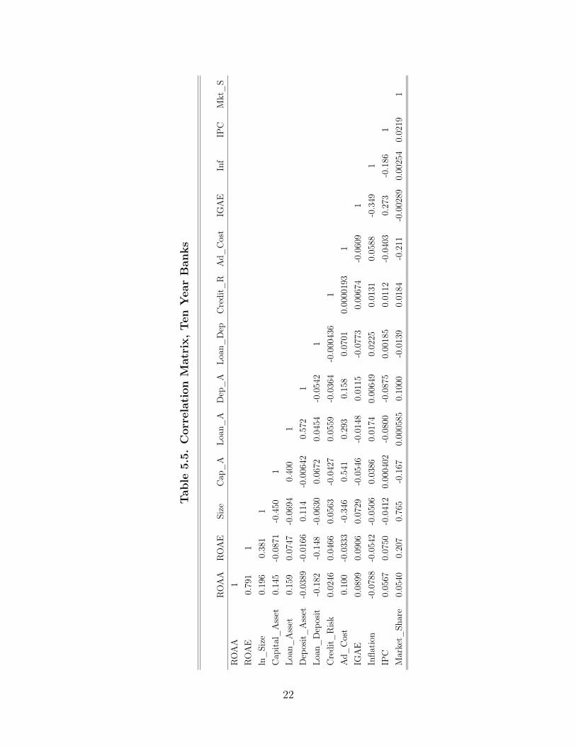
The following tables show the correlation between the profits estimators and theindependent variables used in the model. Three tables are presented, one for each dataset used in the model. It is clear that non of the explanatory variables used, has a highcorrelation with others in order to be concerned about a multicollinearity issue.Furthermore, it is worth mentioning two specific cases, the size of the bank and theadministrative costs. The former appears to be positively correlated with profits,having one of the largest coefficients; the latter has one of the highest negativecorrelative values with profits, in the Six Year Banks data base. Notwithstanding, withthe other data bases the correlation values of administrative costs with profits aremixed; being, as expected, negative with ROAE; but having a counter intuitive resultwith ROAA since the value resulted to be positive (although very small).

The four external variables, namely, IGAE, Inflation, IPC and Market Share, allseem to be consistent in all cases. IGAE, IPC and Market Share, all three appear to bepositively correlated with profits, albeit with a relatively small degree. Inflation, in the

19

three cases has a negative sign, nevertheless, the degree is very close to zero, allowing usto consider that it has no correlation with profits.

20

Tab

le5.

4.C

orre

lati

onM

atri

x,Si

xY

ear

Ban

ks

RO

AA

RO

AE

Size

Cap

_A

Loan

_A

Dep

_A

Loan

_D

epC

redi

t_R

Ad_

Cos

tIG

AE

Inf

IPC

Mkt

_S

RO

AA

1R

OA

E0.

820

1ln

_Si

ze0.

258

0.42

81

Cap

ital_

Ass

et-0

.154

-0.2

49-0

.516

1Lo

an_

Ass

et0.

113

0.01

35-0

.133

0.37

91

Dep

osit_

Ass

et0.

0159

0.00

902

0.13

5-0

.023

30.

540

1Lo

an_

Dep

osit

-0.1

12-0

.118

-0.0

564

0.05

590.

0421

-0.0

495

1C

redi

t_R

isk0.

0146

0.03

670.

0503

-0.0

360

0.05

15-0

.036

2-0

.000

505

1A

d_C

ost

-0.4

25-0

.355

-0.4

220.

642

0.22

60.

0644

0.04

540.

0007

141

IGA

E0.

119

0.09

270.

0625

-0.0

496

-0.0

0141

0.01

12-0

.073

90.

0067

5-0

.086

51

Infla

tion

-0.0

843

-0.0

507

-0.0

336

0.03

000.

0010

10.

0078

90.

0214

0.01

220.

0642

-0.3

481

IPC

0.05

360.

0679

-0.0

167

-0.0

148

-0.0

965

-0.0

866

0.00

181

0.01

06-0

.057

90.

273

-0.1

831

Mar

ket_

Shar

e0.

0767

0.21

00.

745

-0.1

78-0

.010

90.

115

-0.0

128

0.01

71-0

.193

-0.0

0418

0.00

597

0.02

461

21

Tab

le5.

5.C

orre

lati

onM

atri

x,Ten

Yea

rB

anks

RO

AA

RO

AE

Size

Cap

_A

Loan

_A

Dep

_A

Loan

_D

epC

redi

t_R

Ad_

Cos

tIG

AE

Inf

IPC

Mkt

_S

RO

AA

1R

OA

E0.

791

1ln

_Si

ze0.

196

0.38

11

Cap

ital_

Ass

et0.

145

-0.0

871

-0.4

501

Loan

_A

sset

0.15

90.

0747

-0.0

694

0.40

01

Dep

osit_

Ass

et-0

.038

9-0

.016

60.

114

-0.0

0642

0.57

21

Loan

_D

epos

it-0

.182

-0.1

48-0

.063

00.

0672

0.04

54-0

.054

21

Cre

dit_

Risk

0.02

460.

0466

0.05

63-0

.042

70.

0559

-0.0

364

-0.0

0043

61

Ad_

Cos

t0.

100

-0.0

333

-0.3

460.

541

0.29

30.

158

0.07

010.

0000

193

1IG

AE

0.08

990.

0906

0.07

29-0

.054

6-0

.014

80.

0115

-0.0

773

0.00

674

-0.0

609

1In

flatio

n-0

.078

8-0

.054

2-0

.050

60.

0386

0.01

740.

0064

90.

0225

0.01

310.

0588

-0.3

491

IPC

0.05

670.

0750

-0.0

412

0.00

0402

-0.0

800

-0.0

875

0.00

185

0.01

12-0

.040

30.

273

-0.1

861

Mar

ket_

Shar

e0.

0540

0.20

70.

765

-0.1

670.

0005

850.

1000

-0.0

139

0.01

84-0

.211

-0.0

0289

0.00

254

0.02

191

22

Tab

le5.

6.C

orre

lati

onM

atri

x,C

ompl

ete

Yea

rB

anks

RO

AA

RO

AE

Size

Cap

_A

Loan

_A

Dep

_A

Loan

_D

epC

redi

t_R

Ad_

Cos

tIG

AE

Inf

IPC

Mkt

_S

RO

AA

1R

OA

E0.

837

1ln

_Si

ze0.

229

0.28

81

Cap

ital_

Ass

et0.

221

-0.0

787

-0.2

461

Loan

_A

sset

0.34

00.

226

0.15

00.

218

1D

epos

it_A

sset

0.04

010.

0341

0.24

90.

0215

0.66

91

Loan

_D

epos

it-0

.102

-0.0

813

-0.0

988

0.15

20.

0094

9-0

.068

71

Cre

dit_

Risk

0.04

830.

0411

0.06

37-0

.070

00.

0588

-0.0

418

-0.0

0407

1A

d_C

ost

0.07

74-0

.014

0-0

.187

0.21

60.

186

0.30

10.

0144

-0.0

0877

1IG

AE

0.04

500.

0698

0.04

670.

0131

-0.0

286

-0.0

403

-0.0

0020

90.

0082

5-0

.016

91

Infla

tion

-0.0

447

-0.0

310

-0.0

733

-0.0

178

0.03

590.

0319

0.04

060.

0161

0.01

58-0

.358

1IP

C0.

0555

0.11

2-0

.156

-0.0

270

-0.0

682

-0.0

650

-0.0

358

0.01

910.

0012

70.

314

-0.1

981

Mar

ket_

Shar

e0.

116

0.16

00.

772

-0.0

863

0.11

10.

235

-0.0

216

0.02

19-0

.125

-0.0

0206

0.00

0590

0.00

732

1

23

Chapter 6

Econometric Model

Given that the data based had a comprehensible amount of time in monthly paneldata, a fixed effects model was proposed to address the main question of this work. Thistype of approaches aim at controlling for time invariant factors in order to examine howthe dependent and independent variables relate within an entity, in this case, a bank.In the previous sections, the predictors were defined and it was argued how they couldbe of use when explaining profits. They were chosen from an internal, market, andmacroeconomic perspective in order to elucidate how banks’ profitability changes.

The fixed effects model has been widely used in these type of studies since its mainadvantage relies on the fact that it accounts for movements in the dependent variableonly through time changing variables; meaning that all other constant explanatoryvariables are withdrawn or controlled for. Each bank has unique characteristics thatmake it differ from others, such as assets, debts, loans, internal costs or market share.These are directly observable and measurable variables; we can actually calculate howmuch assets a bank possess, or how many loans has the bank given and therefore we areable to determine their evolution, growth or shrinkage overtime. Nonetheless, therecould be other time invariant factors, or some unobserved variables that we are unableto measure that could possibly affect the profitability of the bank. If those effects exist,they would be desirable to control for in order to extract the net effect out of ourpredictors. This is the main reason why the fixed effects model is extremely useful, itallow us to control for those variables that we are able to observe and measure; andfurthermore, for those that we can’t. This would not be possible in a purely crosssectional data or time series analysis; in panel data we have both, a pool of individualsand their characteristics, all measured across time.

24

Lets consider the simplest example, imagine we have a sample of N banks in ahighly competitive market, operating under the similar internal circumstances, such asasset management, debt, loans and costs; but with some regional differences. Forinstance, suppose distance to work varies considerably across banks but is timeinvariant, thus fixed over time (assume that individuals are employed at the sameworkplace for several periods of time). If we believe that being closer to work couldpotentially have effects on a workers productivity, then we are assuming a correlationbetween internal variables and distance to work. In this sense, a fixed effect model isideal, since the distance could be considered as a fixed effect across time, but differentcross-sectionally. If distance to work is time invariant, then, it will have no effect onprofits; instead, changes in profits movements will be given by other causes.

There are, however, situations in which it is suspected that some fixed effects areactually not correlated with the explanatory variables. This is the main differencebetween the fixed effects and the random effects models, if there is a suspicion that theunobserved variables are uncorrelated with the explanatory variables, then those effectsare precisely that, random. Hence, a random effects model should be employed. Whenusing fixed effects, even though we cannot observe them, we suspect they are correlatedwith our predictors, they are time invariant and therefore possible to control for.

The simple univariate theoretical equation for the fixed effects model may be writtenas:

yit = �xit + uit

Where yit represents the independent variable, xit the explanatory variables with itsrespective coefficient �, and uit the error term.

Given that we are only accounting for time changing variables effects, the error termbecomes particularly important since it may allow us to search for those time invariantimpacts, thus, fixed effects. In this sense, uit may be decomposed into two different terms:

uit = ↵i + ✏it

Where ↵i constitutes the time invariant factors, thus fixed, effects; and ✏it the

25

idiosyncratic error term which contains all the information of those effects thatinfluence the independent variable but that could not be accounted for. We assume, ofcourse, that our predictors are not correlated with the idiosyncratic error.

In order to have additional evidence about the type of model more suitable for thedata, this study performed the Hausman test. All the results from the Hausman tests areshown in the Appendix of this work, there is one for every regression made, meaning, foreach regression in the six year bank, ten year banks and complete year banks data bases.As expected, they reinforced and suggested the idea that the fixed effects model was moresuitable for the econometric analysis than the random effects model. The Hausman testis perform to detect endogeneity, it focuses on the fact that the error term for each entityis uncorrelated with the error term of the others. However, if it is, then the estimationwill be biased and the fixed effects model should not be used. We have a sample ofdifferent banks, in which case we may be able to assume that the error terms with oneanother should not be correlated. In order to assess this proposition the Hausman testwas performed; as expected, the results rejected the hypothesis that the available datawas more suited with random effects than with fixed effects, meaning that the error termfor each particular bank was statistically uncorrelated with the others. The followingequation was estimated for three different data bases, one including the banks that after2006 had at least six years of information, another one that incorporates banks with atleast ten years of data after 2006, and a third one encompassing only the banks that hadall data available for the period 2000-2019.

profitability it = �0 + �1ln_Sizeit + �2Capital_Assetit + �3Loan_Assetit

+ �4Deposit_Assetit + �5Loan_Depositit + �6Credit_Riskit + �7Ad_Costit

+ �8Igaeit + �9Inflationit + �10IPCit + �11Market_Shareit + uit

Where profitability was measured by Return on Average Assets and Return onAverage Equity for each bank i in every period t.

Moreover, we made a test to see whether or not the time dummy variables weresignificant, this is, to address if all coefficients for all years were jointly equal to zero or

26

not. The test suggested the need for Time Fixed effects only for the models usingROAE as a dependent variable, meaning that we reject the null hypothesis of the testthat all coefficient for all the available years are jointly zero. However, when the testwas applied to the model with clusters, the null hypothesis was rejected for both ROAAand ROAE, encouraging the use of the Time Fixed Effects model, therefore it was usedin the present study. The main difference between Fixed Effects and Time Fixed Effectsis that the latter controls for those factors affecting all individuals equally. In this case,inflation and economic growth will have the same effect in all agents in every period. Itis not possible for one bank to be affected by one inflation and another bank by anotherinflation, it is the same for both. Fixed effects considers time invariant effects, thusfixed, where every agent is affected by the variable in the same way in every period butdifferently cross-sectionally. It is worth mentioning that the tables shown for the timefixed effects model estimations, in the results section, are not shown completely, onlythe variables we are interested in appear. This is because when estimating time fixedeffects to find impacts on profits, one dummy variable is created for each period of time,and we are not interested in the coefficients of those dummy variables, but rather in theconsistency of the results of our explanatory variables.

In addition, as an exploratory analysis, the information from the complete yearbanks data base was divided in three different samples in order to examine the bankingsector in Mexico before (2001-2006), during (2007-2009) and after (2010-2019) thefinancial crisis. The Fixed Effects and the Time Fixed effects models were used forthese three stages. We had three different data bases; however, only the data base withthe complete banks information (2000-2019) was suitable for the analysis. Both the sixyear banks and the ten year banks data bases were not appropriate since the sampleswere unbalanced since many of the banks were not present in the period before thecrisis. Moreover, some banks in those data bases would have had very limitedobservations, this is also due to the fact that many banks in those data bases did nothave any information for the years previous to the financial crisis; therefore, thisinformation was omitted. The complete banks data base did not have these issues, thebanks had basically the same observations for the whole period and they were allpresent before, during and after the financial crisis, although one of its drawbacks is thelack of data, given that we divided the sample in three sub-samples.

The following tables show the list of banks utilized in each regression for every period.

27

Table 6.1. Six Year Banks, Period of Regression: 2007-2019

Abc Capital Banco Walmart Consubanco J.P. MorganAccendo Banco Bancoppel Credit Suisse MonexActinver Bank of America Deutsche Bank Mufg BankAfirme Bankaool Forjadores MultivaAmerican Express Banorte HSBC SantanderAutofin Banregio Inbursa ScotiabankBanamex Bansi ING The Bank of New York MellonBanca Mifel Barclays Inmobiliario Mexicano Ve por masBanco Ahorro Famsa BBVA Bancomer Interacciones Volkswagen BankBanco Azteca Biafirme Intercam BancoBanco Base Cibanco InvexBanco del Bajío Compartamos Ixe

Table 6.2. Ten Year Banks, Period of Regression: 2007-2019

Abc Capital Banco del Bajío Compartamos MonexAccendo Banco Bancoppel Consubanco Mufg BankActinver Bank of America Credit Suisse MultivaAfirme Banorte Deutsche Bank SantanderAmerican Express Banregio HSBC ScotiabankAutofin Bansi Inbursa Ve por masBanamex Barclays Interacciones Volkswagen BankBanca Mifel BBVA Bancomer Intercam BancoBanco Ahorro Famsa Biafirme InvexBanco Azteca Cibanco J.P. Morgan

Table 6.3. Complete Year Banks, Period of Regression: 2001-2019

Accendo Banco Banco del Bajío Credit Suisse J.P. MorganAfirme Bank of America Deutsche Bank MonexAmerican Express Banorte HSBC Mufg BankBanamex Banregio Inbursa SantanderBanca Mifel Bansi Interacciones ScotiabankBanco Azteca BBVA Bancomer Invex Ve por mas

28

Chapter 7

Results

The original data suggested the presence of heteroscedasticity, and since thetheoretical model assumes homoscedasticity we had to control for it; in fact, data alsopresented serial autocorrelation. The previous conclusions were drawn out of thedifferent tests we performed, namely: the Wald test to detect heteroscedasticity, inwhich the null hypothesis suggests the presence of homoscedasticity, which, in everyregression made, appeared to be rejected; the Wooldridge test for serial autocorrelationin panel data, in which the null hypothesis suggest no serial correlation, which, in everycase we rejected it. All results are shown in the Appendix, there is one table for everyregression made, meaning, for each regression in the six year bank, ten year banks andcomplete year banks data bases, for every one of the tests. To address these particularissues and in order for our results to be robust, the fixed effects models had to be doneconsidering clusters, where the cross-sectional variable used was Banks. This method ishelpful to control for autocorrelation and heteroscedasticity. In this sense, our standarderrors which are shown in parenthesis in every table, are robust for autocorrelation andheteroscedasticity.

Therefore, several different estimations were made. As mentioned before, we hadthree different data bases, one which considered the banks with at least six years ofdata after 2006, another one with banks that had information for at least ten years,after 2006 as well, and one last one that comprised the Banks that possessed completedata, namely 2001-2019. For each of the data bases ROAA and ROAE were used asdependent variables for different estimations. For each, the fixed effects model and thetime fixed effects model were calculated with the raw information, meaning that theywere done directly, not controlling for heteroscedasticity or autocorrelation. Then, the

29

same two models for the two dependent variables were estimated, but now controllingfor both issues with the clusters method, using Banks as our cross-sectional variable.

The results in this work were found to be consistent across the two different types ofmodels, through the three different data bases and in the two profits approximations.All estimations presented below belong to the calculations carried out with robuststandard errors, this is, errors resulting from the clusters method. Although it is worthmentioning that for the first type of models, namely those done directly, withoutcontrolling for heteroscedasticity or autocorrelation, results were fairly consistent withthe literature. Having the size, in general, as significant and positive, costs negative andsignificant for most cases, credit risk being negative and significant (although with afairly low coefficient), IPC being positive and significant in most cases, all which areconsistent with the robust estimations for fixed effects and time fixed effects they are allshown in the appendix of this work.

In the clusters regressions, both in the fixed effects and the time fixed effectsmodels, the liquidity term, measured by the loan-deposit ratio, was negative andsignificant in practically all cases. However, its impact was nearly zero. Comparing ourresults with those that Chavarín (2016) found for Mexico in the period 2007-2013 in hisdynamic panel regression model, we are able to observe that his results on this variableappeared to be insignificant in virtually all cases with robust standard errors.

The credit risk, measured by the preventive estimation of credit risk over totalloans, in all cases, namely in both profits approximations, across all models and databases, had consistent results with those found in the literature; we must mention thatthey were specially robust for ROAE relative to those obtained with ROAA.Coefficients were negative and significant, with a particular higher effect in the database containing the banks with the most abundant data, this is, the one that comprisemostly the bigger banks, suggesting that they have more sensibility to credit risk thansmaller ones. This could be due to the fact that larger banks have more clients withmore voluminous contracts which lead to higher risk if one of them defaults. This resultdeviates with what Chavarín (2016) found for Mexico, where he concluded that creditrisk, measured by provision for loan losses to total loans, was insignificant in explainingprofits. It is also possible that results are different because in some estimations theauthor did not take into account those banks with the greatest losses, which in fact,

30

could potentially deviate the credit risk effects on profits. As stated previously resultswere consistent with those found in the literature, in both significance and sign,although in general our coefficients were smaller. For example, Dietrich and Wanzenried(2014) found credit risk, measured by loan loss provisions relative to total assets, to besignificant and negative in most cases. The same is true for the credit risk results inCapraru and Ihnatov (2014) and Athanasoglou et al. (2008) were the impact on profitswas, in general, significant and negative. What Adelopo et al. (2018) found for creditrisk, measured by the net loans to deposits and short-term funding, was also a negativerelation but with higher coefficient than the ones obtained in this work. Petria et al.(2015) had similar results for the European banking sector, but with a coefficient with agreater negative effect of credit risk measured by the ratio of impaired loans to grossloans, specially for the case or ROE.

In relation to the administrative cost, it seems to be the variable with the highestcoefficients, being, as expected, negative and significant for virtually all cases. In bothin ROAA and ROAE this was found to be the case, but the effect seems much larger inROAE. Nonetheless, just for the banks with the largest data set available, namely, the19 years, this variable was found to be insignificant in both fixed effects and time fixedeffects. Chavarín (2016) found for Mexico in 2007-2013, although using operating costs,that this variable was significant (negative), but insignificant when excluding bankswith the largest losses. Adelopo et. al. (2018) also found that these coefficients had anegative impact on profitability; they argue that costs are significant in all periods,namely before, during and after the crisis. This might be the only variable were resultsare, in general, not mixed. For example, other authors estimating costs such as Petriaet. al. (2015), Dietrich and Wanzenried (2014), Al-Harbi (2019); Athanasoglou et. al.(2008); Ally (2014) and Bolarinwa et. al. (2019) all argue that reducing costs will havea positive effect on profits. There is practically no debate on the direction of the results;the magnitude, however, is something that varies over studies.

The last variable that was strongly consistent was IPC, which is the Mexican StockMarket Index calculated with some of the biggest and most liquid firms in Mexico. Asexpected, it was positive and significant for most cases 1, and it was specially robust for

1Interpretation for IPC in the Time Fixed Effects Model was omitted because all firms are facingthe same IPC, and this model controls for variables affecting all individuals equally, therefore itsinterpretation is not quite as accurate as in the entity fixed effects model.

31

ROAE. None of the revised literature used a stock market index as an independentvariable, therefore there is no practical comparison about the results. However, it isworth noting that as the data bases include banks with more information, and speciallywhen considering only those banks with 19 years of data, which are associated with thelargest ones in our data set, IPC’s significance and effect become stronger. Theseresults are found to be consistent with the hypothesis that given that larger banks havelarger firms as clients, then it is possible that when the market is rewarding thosecompanies, this has positive effects on the banks profits.

The macroeconomic variables, such as economic growth measured by the GlobalIndicator for Economic Activty (IGAE), and inflation rate, had no statisticallysignificant results for the six nor ten year data bases. Considering the banks with 19years of information, which are more associated to the larger banks, inflation had anexceptionally positive and significant effect, specifically in ROAE. For Mexico, Chavarín(2016) did not use the inflation as an independent variable, therefore no directcomparison can be held; nevertheless, for GDP he found it to be, in general, positivelyaffecting profits. Literature has mixed opinions about the effects of inflation in profits.For example, Adelopo et. al. (2018) found that inflation has in general a negativeimpact on profits, although it is also argued that its effect vary when considering theperiod before, during or after the crisis. On contrast, Dietrich and Wanzenried (2014)using information from Fitch-IBCA Bankscope (BSC) database, and estimating amodel for 118 countries, found this effect to be positive and significant effect on profitsfor low- and middle-income countries, where Mexico could be placed according toChavarín (2016), but not for the high-income countries. As mentioned before, theinterpretation of the coefficients resulted in the Time Fixed effects model are ignored.This is due to the fact that the model controls for variables that influence all entitiesequally, as it is, macroeconomic variables do affect them in the same way. There is nobank experiencing a different inflation or economic growth than other.

At last, similar results where found for Market share, as the information grows, andsmaller banks are not considered in the data, market share appears to be significant andnegative, this is true for ROAE solely in complete year banks data base under the TimeFixed Effects model. This would mean that an increase in assets, relative to those inthe market, actually have an inverse effect on profits. This result is quite interestingsince it suggests that due to an increase in the market share of the bank, which can be

32

seen as higher concentration in the market, actually reduces the banks profits. Thisresult evinces that competition might actually have positive effects on banks’profitability. Adelopo et al. (2018) found market power, measured in the same way, tohave mixed results, depending on the period of analysis, previous, during or post crisis.Furthermore, Petria et al. (2015) observed the same results as this work for banks inthe European Union, in the period from 2004-2011. Same as this study, they provideevidence that concentration in the market reduces profits, meaning that competitionactually has positive impact in the banks’ profitability. In contrast, Chavarín (2016) forMexico in 2007-2013 found market share to be insignificant in practically all cases.

Results showed that competition could possibly have positive effects on banksprofits, this could be due to the fact that in the banking sector banks are actively incontact with each others in the interbank market. Competition may provide means toapproach clients in a more efficient way; if an agent is looking for prices (generallyspeaking, for any financial instrument) in several banks, this could encourage them tolower the prices in order to keep the clients. We must consider that banks are inside amarket where they have other banks as competitors and prices still play a crucial role inthe distribution of the market in terms of competitiveness, meaning market share ormarket power. Furthermore, each bank has its own way to address counterparty creditrisk, in this sense some banks may be trying to compete with others by reducing prices,but their risk management must follow a betterment in performance and efficiency aswell; there is no point in reducing prices if risk taken by the bank are too high andexpected gains are not as elevated. These increases in efficiencies could potentially be asource of the enlargement in profits. A further and deeper analysis in marketconstraints, barriers of entry, efficiencies, must be held to find a more conclusiveargument; however, this is not the main scope of this work.

The results for size found in both models are, in general, consistent with what hasbeen found in the literature. They indicate that the size of the bank, measured as thenatural logarithm of the total assets of the bank, have a positive and significant effect inprofits, specially for ROAE and for the banks with the complete data, associated withonly the largest banks. In the Fixed Effects model, size was significant and positivewith a relatively high coefficient for the data base comprising the banks with the mostdata, which is associated with the larger banks. They were all positive and significantand also higher for ROAE than for ROAA. In the Time Fixed Effects model, the

33

coefficient was positive and significative in all cases for ROAE, but ROAA wasstatistically significant only in the 19 year banks data base. As Adelopo et al. (2018)found in a fixed effects model for the period 1999 to 2013, banks size was significant forall periods, namely before, during and after the crisis; Chavarín (2016) for Mexico inthe period of 2007-2013 and Menicucci and Paolucci (2016) applying a linear regressionmodel on the pooled sample for European banks in 2009-2013, found this result to beconsistent with theirs, arguing that total assets have a positive impact on profits.Adelopo et al. (2018) observed that profits could be either positively or negativelyaffected by size for two main factors. As banks grow larger they become more profitablebecause of economies of scale, but as they do, they also tend to get higher costs andbecome harder to manage. There are however, some studies in the literature that founddifferent results, Dietrich and Wanzenried (2014) results for example, they show noevidence that larger banks are more profitable for ROAA but they do have a positiveeffect with ROAE as the dependent variable. Finally we could mention Capraru andIhnatov (2014) that found this predictor to have a negative influence on profts, andAl-Harbi (2019) who observed an insignificant coefficient.

In relation with the Loan Asset ratio and the Deposit Asset ratio, they wereinsignificant in every single scenario, for both the time fixed effects the fixed effectsmodels. These ratios were not calculated by Chavarín (2016); however, Menicucci &Paolucci (2016) for the European banking sector during the period 2009-2013, foundDeposits ratio to be positive and significant and Loans Ratio was actually insignificantfor both ROA and ROE.

The capital asset ratio has positive and significant effect, although uniquely for thebanks with the largest data history and for ROAA, both in the time fixed effects andthe fixed effects model. This result seems to be consistent with the literature, forexample Menicucci & Paolucci (2016) and Öhman and Yazdanfar (2018) found similarresults, were capital strength appeared to be an important determinant, having ingeneral a positive effect on profits. Chavarín (2016) for Mexico also found this to be thecase, although with higher values for the coefficients, than our study. Petria et al.(2015) found it to be insignificant, arguing that two things happen, high capitaladequacy could possibly reduce the risk of a bank, and also because banks do not takeadvantage from the leverage effect. Finally Adelopo et al. (2018) argue that its effectchanges depending on the period analyzed (before, during or after the crisis).

34

One of the main contributions of this study is the inclusion of the Mexican StockMarket Index, namely, the IPC into the analysis of determinants. Considering theresults, we could assert that the relation between the IPC and the bank’s profits is nontrivial. Companies that rely strongly on the performance of these indicators andmarkets will potentially have a larger impact on the banks profits. There is, however astrong drawback these kind of relations. Since they have a positive relation, wheneverthe market improves, the banks will do as well, and profits will rise; on the contrary, ifthe situation deteriorates, then profits will most likely decrease. The results found inthis analysis suggests a positive relation between IPC and profits, meaning apro-cyclical association with the market, which at the same time, advocates for keenand sharp hedging strategies. Having extraordinarily large profits is not as usual ashaving substantial losses, the current situation with the pandemic caused by COVID-19showed it pretty well. Once the biological anomaly became a global issue, marketsstarted to react, the stock markets were dramatically damaged and economies wereseverely injured. These type of situations exhort the best performance out of thefinancial institutions since the economy relies greatly on them. There are, however,priorities that must be evaluated by decision makers, in order to address this crisis. Wecould consider the substantial quantity of firms that went under bankruptcy when thecrisis arrived, which aggravate the counterparty credit risk that banks face. Thisunmasks two underlying issues, one is that banks could try to lend more, increase thecredits, or extend them in order to get late but more secure payments, to help there-bounce of the economy; nonetheless, this could potentially result in losses given thecredit risk. On the other hand they could try to protect their assets, reduce credits, orincrease charges and commissions and take a more secure position to avoid losses; eitherway decisions are absolutely non trivial. With the results found in the analysis andconsidering the current crisis, it is naturally to anticipate that these unexpected lossesexperienced by the financial system, which most likely will be manifested by the IPCindicators, will impact negatively on banks profits; in future analysis the magnitudecould be evaluated with the coefficients obtained in the present work.

35

Table 7.1. Fixed Effects Regression, Period: 2007-2019, Clusters, Six YearBanks

(1) (2) (3) (4)ROAA ROAA ROAE ROAE

ln_Size -0.00117 -0.00144 0.0281 0.0267(0.00476) (0.00513) (0.0200) (0.0205)

Capital_Asset 0.00597 0.00669 0.0486 0.0537(0.0407) (0.0430) (0.165) (0.168)

Loan_Asset 0.0316 -0.00218(0.0302) (0.0774)

Deposit_Asset -0.0196 -0.0332(0.0308) (0.0846)

Loan_Deposit -0.00000397*** -0.00000360*** -0.0000123*** -0.0000120***(0.000000596) (0.000000264) (0.00000177) (0.00000114)

Credit_Risk -0.0000738 0.00000428 -0.000648*** -0.000578***(0.0000896) (0.0000376) (0.000226) (0.0000769)

Ad_Cost -0.636*** -0.636*** -0.997*** -0.990***(0.0670) (0.0693) (0.171) (0.165)

IGAE 0.0237 0.0274 0.0115 0.0100(0.0292) (0.0303) (0.135) (0.138)

Inflation -0.00794 -0.0109 0.247 0.233(0.0512) (0.0524) (0.213) (0.205)

IPC 0.00448 0.00292 0.0496*** 0.0517***(0.00459) (0.00433) (0.0175) (0.0174)

Market_Share -0.122 -0.142 0.0467 0.133(0.114) (0.101) (0.430) (0.363)

_cons 0.0645 0.0737 -0.140 -0.143(0.0568) (0.0575) (0.228) (0.231)

N 5580 5580 5580 5580R2 0.732 0.727 0.373 0.371adj. R2 0.731 0.727 0.371 0.370F 67724.2 33567.4 54584.5 52785.6p 5.55e-85 2.42e-77 5.14e-83 1.80e-81

Standard errors in parentheses

* p<0.10, ** p<0.05, *** p<0.010

36

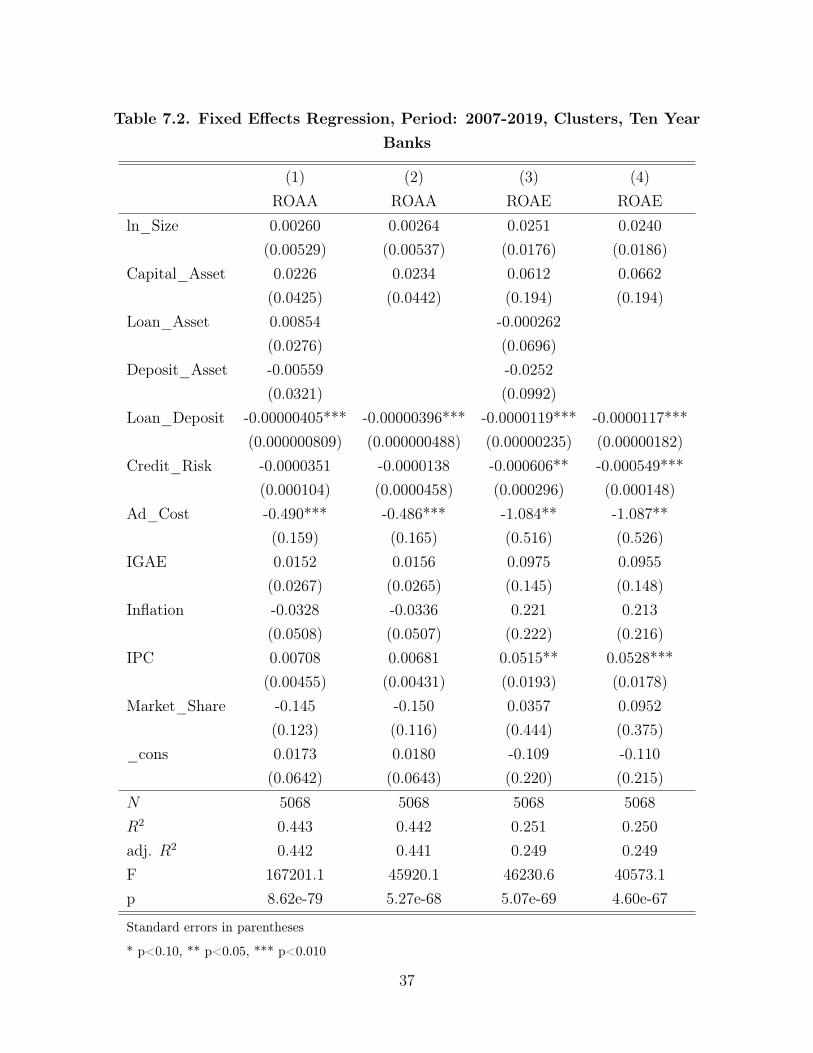
Table 7.2. Fixed Effects Regression, Period: 2007-2019, Clusters, Ten YearBanks

(1) (2) (3) (4)ROAA ROAA ROAE ROAE

ln_Size 0.00260 0.00264 0.0251 0.0240(0.00529) (0.00537) (0.0176) (0.0186)

Capital_Asset 0.0226 0.0234 0.0612 0.0662(0.0425) (0.0442) (0.194) (0.194)

Loan_Asset 0.00854 -0.000262(0.0276) (0.0696)

Deposit_Asset -0.00559 -0.0252(0.0321) (0.0992)

Loan_Deposit -0.00000405*** -0.00000396*** -0.0000119*** -0.0000117***(0.000000809) (0.000000488) (0.00000235) (0.00000182)

Credit_Risk -0.0000351 -0.0000138 -0.000606** -0.000549***(0.000104) (0.0000458) (0.000296) (0.000148)

Ad_Cost -0.490*** -0.486*** -1.084** -1.087**(0.159) (0.165) (0.516) (0.526)

IGAE 0.0152 0.0156 0.0975 0.0955(0.0267) (0.0265) (0.145) (0.148)

Inflation -0.0328 -0.0336 0.221 0.213(0.0508) (0.0507) (0.222) (0.216)

IPC 0.00708 0.00681 0.0515** 0.0528***(0.00455) (0.00431) (0.0193) (0.0178)

Market_Share -0.145 -0.150 0.0357 0.0952(0.123) (0.116) (0.444) (0.375)

_cons 0.0173 0.0180 -0.109 -0.110(0.0642) (0.0643) (0.220) (0.215)

N 5068 5068 5068 5068R2 0.443 0.442 0.251 0.250adj. R2 0.442 0.441 0.249 0.249F 167201.1 45920.1 46230.6 40573.1p 8.62e-79 5.27e-68 5.07e-69 4.60e-67

Standard errors in parentheses

* p<0.10, ** p<0.05, *** p<0.010

37

Table 7.3. Fixed Effects Regression, Period: 2001-2019, Clusters, CompleteYear Banks

(1) (2) (3) (4)ROAA ROAA ROAE ROAE

ln_Size 0.00384** 0.00388** 0.0338* 0.0341*(0.00175) (0.00173) (0.0176) (0.0171)

Capital_Asset 0.0381*** 0.0457*** -0.101 -0.0385(0.0115) (0.0109) (0.249) (0.262)

Loan_Asset 0.0171 0.110(0.0157) (0.120)

Deposit_Asset -0.0187 -0.167(0.0178) (0.150)

Loan_Deposit -0.00000275*** -0.00000256*** -0.0000108*** -0.00000869***(0.000000435) (0.000000604) (0.00000296) (0.00000199)

Credit_Risk -0.000135*** -0.0000751** -0.00177*** -0.00128***(0.0000398) (0.0000296) (0.000284) (0.000398)

Ad_Cost -0.104 -0.106 -0.768 -0.800(0.183) (0.193) (1.613) (1.697)

IGAE -0.0101 -0.00825 0.0648 0.0752(0.0255) (0.0244) (0.203) (0.200)

Inflation 0.0178 0.0203 0.601** 0.615**(0.0437) (0.0423) (0.289) (0.281)

IPC 0.00986** 0.00990** 0.121*** 0.125***(0.00382) (0.00422) (0.0349) (0.0375)

Market_Share -0.0726 -0.0728 -0.956 -0.913(0.0665) (0.0646) (0.674) (0.663)

_cons -0.0288* -0.0311* -0.196 -0.234(0.0149) (0.0155) (0.154) (0.176)

N 4824 4824 4824 4824R2 0.121 0.105 0.094 0.082adj. R2 0.119 0.103 0.092 0.080F 52545.0 48761.8 16573.6 25563.9p 1.18e-47 9.37e-47 6.83e-42 1.57e-43

Standard errors in parentheses

* p<0.10, ** p<0.05, *** p<0.010

38

Table 7.4. Time Fixed Effects Regression, Period: 2007-2019, Clusters, SixYear Banks

(1) (2) (3) (4)ROAA ROAA ROAE ROAE

ln_Size -0.00310 -0.00445 0.0884** 0.0862**(0.00787) (0.00721) (0.0380) (0.0370)

Capital_Asset 0.0000216 -0.00319 0.283 0.270(0.0469) (0.0461) (0.244) (0.233)

Loan_Asset 0.0308 0.0274(0.0308) (0.0771)

Deposit_Asset -0.0192 0.00159(0.0317) (0.0812)

Loan_Deposit -0.00000403*** -0.00000368*** -0.0000108*** -0.0000106***(0.000000612) (0.000000287) (0.00000212) (0.00000151)

Credit_Risk -0.0000600 0.0000257 -0.000789*** -0.000752***(0.0000852) (0.0000419) (0.000222) (0.0000851)

Ad_Cost -0.636*** -0.636*** -0.932*** -0.938***(0.0693) (0.0703) (0.152) (0.149)

IGAE 0 0 0 0(.) (.) (.) (.)

Inflation 0 0 0 0(.) (.) (.) (.)

IPC 0.00940 0.00802 0.103** 0.102**(0.00651) (0.00637) (0.0399) (0.0400)

Market_Share -0.0897 -0.0947 -0.708 -0.736(0.111) (0.112) (0.484) (0.466)

_cons 0.0826 0.102 -0.730* -0.693*(0.0920) (0.0768) (0.414) (0.390)

N 5580 5580 5580 5580R2 0.734 0.730 0.414 0.414adj. R2 0.726 0.722 0.397 0.396

Standard errors in parentheses

* p<0.10, ** p<0.05, *** p<0.010

39

Table 7.5. Time Fixed Effects Regression, Period: 2007-2019, Clusters, TenYear Banks

(1) (2) (3) (4)ROAA ROAA ROAE ROAE

ln_Size 0.00320 0.00297 0.0872** 0.0857**(0.00896) (0.00848) (0.0344) (0.0327)

Capital_Asset 0.0260 0.0255 0.295 0.282(0.0524) (0.0531) (0.265) (0.248)

Loan_Asset 0.00911 0.0191(0.0287) (0.0711)

Deposit_Asset -0.00470 0.0122(0.0320) (0.0918)

Loan_Deposit -0.00000407*** -0.00000398*** -0.0000106*** -0.0000106***(0.000000782) (0.000000463) (0.00000265) (0.00000207)

Credit_Risk -0.0000252 -0.00000273 -0.000745** -0.000744***(0.000105) (0.0000423) (0.000290) (0.000131)

Ad_Cost -0.484*** -0.480*** -0.928* -0.924*(0.166) (0.172) (0.495) (0.508)

IGAE 0 0 0 0(.) (.) (.) (.)

Inflation 0 0 0 0(.) (.) (.) (.)

IPC 0.0122* 0.0119* 0.115*** 0.114***(0.00611) (0.00630) (0.0389) (0.0386)

Market_Share -0.144 -0.149 -0.721 -0.757(0.114) (0.116) (0.481) (0.460)

_cons 0.00928 0.0134 -0.731* -0.700*(0.107) (0.0968) (0.391) (0.353)

N 5068 5068 5068 5068R2 0.448 0.447 0.303 0.302adj. R2 0.430 0.429 0.280 0.279

Standard errors in parentheses

* p<0.10, ** p<0.05, *** p<0.010

40

Table 7.6. Time Fixed Effects Regression, Period: 2001-2019, Clusters,Complete Year Banks

(1) (2) (3) (4)ROAA ROAA ROAE ROAE

ln_Size 0.00847** 0.00774** 0.0791** 0.0771**(0.00345) (0.00356) (0.0344) (0.0364)

Capital_Asset 0.0588*** 0.0624*** 0.0973 0.141(0.0159) (0.0190) (0.328) (0.354)

Loan_Asset 0.0203 0.138(0.0168) (0.122)

Deposit_Asset -0.0148 -0.124(0.0153) (0.112)

Loan_Deposit -0.00000240*** -0.00000237*** -0.00000718** -0.00000645**(0.000000553) (0.000000686) (0.00000299) (0.00000304)

Credit_Risk -0.000152*** -0.0000904*** -0.00199*** -0.00153***(0.0000388) (0.0000301) (0.000279) (0.000381)

Ad_Cost -0.0800 -0.0823 -0.488 -0.503(0.175) (0.182) (1.521) (1.574)

IGAE 0 0 0 0(.) (.) (.) (.)

Inflation 0 0 0 0(.) (.) (.) (.)

IPC -0.00900 -0.00630 -0.00669 0.00837(0.00859) (0.00788) (0.0860) (0.0870)

Market_Share -0.135 -0.135 -1.681* -1.689*(0.0824) (0.0871) (0.880) (0.905)

_cons -0.0756** -0.0683** -0.687** -0.677*(0.0301) (0.0309) (0.328) (0.356)

N 4824 4824 4824 4824R2 0.161 0.144 0.164 0.155adj. R2 0.121 0.103 0.123 0.114

Standard errors in parentheses

* p<0.10, ** p<0.05, *** p<0.010

41

7.1 Before (2001-2006), During (2007-2009) and After(2010-2019) the Financial Crisis EconometricResults

Since the literature is very limited for Mexico, the current sub-section elaborates anexploratory analysis of the determinants of profitability in the mexican baking sector inthree stages, before (2001-2006), during (2007-2009) and after (2010-2019) the financialcrisis. This analysis is performed in order to provide an overview of the different stages.It is not an exhaustive analysis of the financial crisis and its effects in the bankingsector in Mexico, it is exploratory and it encourages other studies to address this issuewith a deeper approach.

As before, all estimations presented below were calculated using robust standarderrors, meaning, errors resulting from the clusters method. Although, it is worthmentioning that the first type of models, namely those done directly, withoutcontrolling for heteroscedasticity or autocorrelation are all shown in the Appendix.Moreover, as previously mentioned, the data base used for this particular approach wasthe complete year banks data base. Fundamentally, we used this data base because thebanks had the same number of observations across all the period (2001-2019) and thepanel was strongly balanced, meaning that basically the same pool of banks werepresent in all the stages. As indicated above, this is something that was not present inthe other data bases. Nonetheless, there are some drawbacks with this particularapproach. First, in contrast with the work of Adelopo et. al. (2018), where theinformation of banks for 15 different countries was used, we only use one, Mexico. Inthis sense, our results are limited given the data, we had one data base andfurthermore, it had to be divided in three different samples, which substantially reducedthe observations per model. Second, not all banks are considered and this reduces theheterogeneity in the sample. The following briefly explores the results obtained fromthe estimation of the models across stages.

The results obtained from the estimation show substantial divergences across thedifferent periods considered, meaning that perhaps the associated determinants varywithin stages. Notwithstanding, some others were very consistent; for example, theassets of the banks played a positive and significant role as a determinant for virtually

42

all periods, although not for all regressions. The loan asset ratio is basicallyinsignificant for all cases and the loan deposit ratio shows a similar behavior as well,although it is significant in two cases during the crisis, and only in the Time FixedEffects Model. In contrast, other variables appeared to be less stable; for example, thecapital-asset ratio seems to have a positive and significant effect before and after thecrisis, but not during the crisis. Something similar happens with the credit risk, wherealmost all coefficients for the stages before and after were significant; nonetheless, themost unusual result is that it was positive before the crisis, but for the subsequentstages, it was negative and significant. Deposits seem to be only significant before thecrisis but not in the other stages. The most unusual and odd results where obtainedfrom the administrative costs, they were not consistent as in the previous estimations.It has some serious unstable and counter-intuitive results. Coefficients are significantand negative in the stage previous to the crisis. Notwithstanding, for the period duringthe crisis coefficients appear to be extraordinarily high, significant and positive, which isextremely odd and counter intuitive. Results show that the cost is negative but notsignificant after the crisis.

Macroeconomic variables, namely IGAE and inflation also varied both in theirmagnitude and significance across periods, in fact, they were only significant during thecrisis, where coefficients were found to be positive for the economic growth and negativefor inflation. The Mexican Stock Market Index, namely the IPC, was also found to besignificant and positive for the period during the crisis, but not for the others. Marketshare had also some very inconsistent results, as before, their coefficients are negativeand statistically significant previous to the crisis; however, during and after results arenot significant.

The results gathered from these sets of samples were neither particularly consistentwith literature, nor with our previous estimations. There appear to be differences acrossstages, specifically, some coefficients suggested the presence of much more higher effectsduring the crisis. However, these results are neither conclusive nor exhaustive. Weencourage future studies to address this question in order to have additional and clearerevidence.

The following tables show the econometric results for the analysis in the periods before(2001-2006), during (2007-2009) and after (2010-2019) the financial crisis.

43

Table 7.7. Fixed Effects Regression, Period: 2001-2006, Before FinancialCrisis, Clusters, Complete Year Banks

(1) (2) (3) (4)ROAA ROAA ROAE ROAE

ln_Size 0.00134 0.00277 0.0870** 0.111***(0.00557) (0.00476) (0.0355) (0.0303)

Capital_Asset 0.0868*** 0.0955*** 0.970 1.118(0.0273) (0.0260) (0.694) (0.715)

Loan_Asset 0.00948 0.151(0.0131) (0.216)

Deposit_Asset -0.0195 -0.325*(0.0165) (0.157)

Loan_Deposit 0.000000854 0.00000123 0.0000172 0.0000233(0.000000682) (0.000000768) (0.0000143) (0.0000141)

Credit_Risk 0.108*** 0.109*** 1.023** 1.039**(0.0265) (0.0265) (0.451) (0.469)

Ad_Cost -0.532** -0.534* -3.594 -3.626(0.254) (0.271) (2.205) (2.561)

IGAE 0.00669 0.00461 0.437 0.399(0.0384) (0.0361) (0.357) (0.378)

Inflation 0.134 0.153 2.611 2.929(0.137) (0.141) (1.796) (1.942)

IPC 0.0108 0.0104 0.128 0.121(0.00646) (0.00646) (0.0746) (0.0752)

Market_Share -0.114* -0.120* -2.430*** -2.540***(0.0629) (0.0591) (0.554) (0.555)

_cons 0.0181 -0.00190 -0.633 -0.974**(0.0643) (0.0550) (0.429) (0.353)

N 1286 1286 1286 1286R2 0.549 0.541 0.412 0.396adj. R2 0.545 0.538 0.407 0.392F . . 25007666.8 33174863.3p . . 3.33e-75 4.62e-76

Standard errors in parentheses

* p<0.10, ** p<0.05, *** p<0.010

44

Table 7.8. Fixed Effects Regression, Period: 2007-2009, During FinancialCrisis, Clusters, Complete Year Banks

(1) (2) (3) (4)ROAA ROAA ROAE ROAE

ln_Size -0.00175 -0.00229 0.0222 0.0129(0.00360) (0.00282) (0.0320) (0.0289)

Capital_Asset 0.0162 0.0167 -0.0999 -0.111(0.0219) (0.0164) (0.158) (0.145)

Loan_Asset -0.00371 0.0218(0.0223) (0.142)

Deposit_Asset 0.00828 0.0451(0.0156) (0.136)

Loan_Deposit -0.00136 -0.00303 -0.00982 -0.0147(0.00538) (0.00214) (0.0328) (0.0201)

Credit_Risk -0.00599 0.00187 -0.537 -0.433(0.0650) (0.0728) (0.475) (0.518)

Ad_Cost 0.283*** 0.286*** 4.329*** 4.353***(0.0778) (0.0810) (1.018) (1.018)

IGAE 0.0319** 0.0300** 0.550*** 0.528***(0.0116) (0.0115) (0.111) (0.123)

Inflation -0.137** -0.133** -0.546 -0.539(0.0583) (0.0592) (0.675) (0.707)

IPC 0.00138 0.00117 0.0430** 0.0385*(0.00235) (0.00183) (0.0177) (0.0188)

Market_Share 0.0837 0.0798 0.707 0.659(0.0632) (0.0607) (0.522) (0.508)

_cons 0.0199 0.0295 -0.330 -0.190(0.0401) (0.0311) (0.366) (0.327)

N 792 792 792 792R2 0.250 0.247 0.516 0.513adj. R2 0.239 0.238 0.509 0.508F 5.699 6.353 50.62 50.52p 0.000396 0.000315 2.03e-12 5.41e-12

Standard errors in parentheses

* p<0.10, ** p<0.05, *** p<0.010

45

Table 7.9. Fixed Effects Regression, Period: 2010-2019, After FinancialCrisis, Clusters, Complete Year Banks

(1) (2) (3) (4)ROAA ROAA ROAE ROAE

ln_Size 0.00589* 0.00661* 0.0221 0.0217(0.00307) (0.00377) (0.0201) (0.0216)

Capital_Asset 0.0761** 0.0840** 0.150 0.179(0.0341) (0.0369) (0.204) (0.193)

Loan_Asset 0.0101 -0.0485(0.0134) (0.0829)

Deposit_Asset -0.0223 -0.112(0.0166) (0.0975)

Loan_Deposit 0.0000133 0.0000262 -0.000151 -0.000120(0.0000211) (0.0000338) (0.000117) (0.000105)

Credit_Risk -0.000112* -0.0000680* -0.000997*** -0.000906***(0.0000635) (0.0000374) (0.000158) (0.000101)

Ad_Cost -0.0534 -0.0342 -0.0251 -0.0466(0.0854) (0.0752) (0.394) (0.439)

IGAE 0.0576 0.0733 0.362 0.554(0.0570) (0.0694) (0.419) (0.556)

Inflation -0.00782 -0.0228 0.385 0.245(0.0452) (0.0548) (0.320) (0.406)

IPC 0.00419 0.00559 0.00550 0.0166(0.00342) (0.00498) (0.0228) (0.0342)

Market_Share -0.0812 -0.0639 -0.263 -0.00197(0.0785) (0.0776) (0.393) (0.263)

_cons -0.0557* -0.0720* -0.115 -0.192(0.0317) (0.0397) (0.222) (0.252)

N 2746 2746 2746 2746R2 0.124 0.095 0.060 0.031adj. R2 0.120 0.092 0.057 0.028F 116225.2 215025.1 39941.8 46721.7p 1.28e-51 3.64e-54 2.77e-46 1.53e-46

Standard errors in parentheses

* p<0.10, ** p<0.05, *** p<0.010

46

Table 7.10. Time Fixed Effects Regression, Period: 2001-2006, BeforeFinancial Crisis, Clusters, Complete Year Banks

(1) (2) (3) (4)ROAA ROAA ROAE ROAE

ln_Size 0.00230 0.00450 0.118 0.153**(0.00593) (0.00513) (0.0845) (0.0700)

Capital_Asset 0.0910** 0.102*** 1.110 1.289(0.0336) (0.0312) (0.851) (0.813)

Loan_Asset 0.00814 0.125(0.0125) (0.195)

Deposit_Asset -0.0174 -0.278*(0.0163) (0.151)

Loan_Deposit 0.000000917 0.00000126 0.0000177 0.0000231(0.000000741) (0.000000809) (0.0000148) (0.0000143)

Credit_Risk 0.108*** 0.109*** 1.005** 1.016**(0.0269) (0.0266) (0.449) (0.456)

Ad_Cost -0.527* -0.523* -3.458 -3.390(0.255) (0.271) (2.106) (2.421)

IGAE 0 0 0 0(.) (.) (.) (.)

Inflation 0 0 0 0(.) (.) (.) (.)

IPC 0.0121 0.0132 0.152** 0.170**(0.00810) (0.00849) (0.0731) (0.0780)

Market_Share -0.122* -0.134* -2.701*** -2.888***(0.0691) (0.0675) (0.783) (0.790)

_cons 0.0133 -0.0143 -0.852 -1.299*(0.0645) (0.0553) (0.900) (0.698)

N 1286 1286 1286 1286R2 0.556 0.551 0.428 0.417adj. R2 0.531 0.526 0.396 0.385

Standard errors in parentheses

* p<0.10, ** p<0.05, *** p<0.010

47

Table 7.11. Time Fixed Effects Regression, Period: 2007-2009, DuringFinancial Crisis, Clusters, Complete Year Banks

(1) (2) (3) (4)ROAA ROAA ROAE ROAE

ln_Size 0.00242 0.000106 0.0810* 0.0519(0.00432) (0.00283) (0.0426) (0.0316)

Capital_Asset 0.0347 0.0302 0.161 0.0880(0.0278) (0.0198) (0.169) (0.136)

Loan_Asset 0.00263 0.106(0.0226) (0.135)

Deposit_Asset 0.0115 0.0603(0.0158) (0.132)

Loan_Deposit -0.00306 -0.00430* -0.0368 -0.0323*(0.00599) (0.00239) (0.0322) (0.0170)

Credit_Risk -0.0321 -0.00802 -0.866** -0.594(0.0597) (0.0741) (0.414) (0.527)

Ad_Cost 0.301*** 0.302*** 4.582*** 4.590***(0.0750) (0.0821) (0.872) (0.899)

IGAE 0 0 0 0(.) (.) (.) (.)

Inflation 0 0 0 0(.) (.) (.) (.)

IPC 0.0101** 0.00835*** 0.133*** 0.112***(0.00366) (0.00242) (0.0336) (0.0277)

Market_Share 0.0789 0.0692 0.541 0.444(0.0639) (0.0612) (0.612) (0.586)

_cons -0.0381 -0.00401 -1.053** -0.650*(0.0495) (0.0320) (0.490) (0.354)

N 792 792 792 792R2 0.302 0.288 0.570 0.557adj. R2 0.261 0.249 0.545 0.533

Standard errors in parentheses

* p<0.10, ** p<0.05, *** p<0.010

48

Table 7.12. Time Fixed Effects Regression, Period: 2010-2019, AfterFinancial Crisis, Clusters, Complete Year Banks

(1) (2) (3) (4)ROAA ROAA ROAE ROAE

ln_Size 0.0126* 0.0136* 0.0560 0.0673(0.00668) (0.00700) (0.0365) (0.0408)

Capital_Asset 0.0953** 0.103** 0.255 0.307(0.0409) (0.0427) (0.245) (0.251)

Loan_Asset 0.0171 -0.00984(0.0161) (0.0711)

Deposit_Asset -0.0180 -0.102(0.0158) (0.103)

Loan_Deposit 0.0000594 0.0000739 0.0000660 0.000178(0.0000434) (0.0000537) (0.000217) (0.000208)

Credit_Risk -0.000122* -0.0000709** -0.00114*** -0.00100***(0.0000640) (0.0000324) (0.000177) (0.000120)

Ad_Cost -0.0556 -0.0295 -0.0485 -0.0238(0.0775) (0.0616) (0.362) (0.362)

IGAE 0 0 0 0(.) (.) (.) (.)

Inflation 0 0 0 0(.) (.) (.) (.)

IPC 0.0150 0.0160 0.0614 0.0898(0.0118) (0.0122) (0.0759) (0.0929)

Market_Share -0.124 -0.127 -0.484 -0.400(0.0861) (0.0931) (0.477) (0.457)

_cons -0.138* -0.153* -0.505 -0.700(0.0785) (0.0797) (0.439) (0.487)

N 2746 2746 2746 2746R2 0.166 0.144 0.111 0.096adj. R2 0.126 0.104 0.068 0.053

Standard errors in parentheses

* p<0.10, ** p<0.05, *** p<0.010

49

Chapter 8

Conclusions

Generally speaking the results could be seen as consistent with what was found inthe literature. Specifically for Mexico, comparing results with those of Chavarín (2016)who addressed this particular research question, conclusions were mixed, some of whichwere consistent but not considerably consistent. This is possibly due for two reasons.First, the approach was different, the author used a dynamic model using the first lag ofthe profits as an explanatory variable, and a random effects model for the staticapproach. In contrast, this study faced the data with a fixed effects model and a timefixed effect model with robust errors for autocorrelation and heteroscedasticity. Second,the period employed by the author comprehended from 2007 to 2013; conversely, thiswork used data from 2007 to 2019 for two sets of data, and an additional one withinformation from 2001 to 2019.

The most consistent explanatory variables coefficients were found in liquidity,measured by the loan deposit ratio; credit risk, measured by preventive estimation ofcredit risk over total loans; administrative costs, and IPC (Mexican Stock MarketIndex). Liquidity had negative and significant effects, although their coefficients werevery close to zero; credit risk had also small coefficients but they were highly significantand negative; the variable of administrative costs was arguably the one with the largestcoefficients, these being negative and significative for virtually all cases. At last, IPCmust be mentioned, its coefficients were highly consistent, having positive andsignificative values for the majority of the models; they also exhibited higher values forthe data base associated with the largest banks and broadest data base (consideringyears). This is consistent with the idea that larger banks may be benefited relativelymore than smaller banks when rewards are being given by the market. All these

50

variables had similar effects across all models, periods, databases (bank types) andprofits approximations (ROAA and ROAE).

In contrast, macroeconomic variables, namely inflation and economic growth, werenot as consistent or significative across models as the previous regressors. They didn’tseem to be fundamental determinants of profits for all types of Banks; apparently onlybigger banks were influenced by them, particularly by inflation. On one hand, theeconomic growth was found to be insignificant for virtually all cases; on the other,inflation had no effect for the data bases comprising solely banks having six and tenyears of data after 2006. However, this effect was sharply increased in both magnitudeand most importantly, significance, when the 19 years data base was considered.Results offered evidence that inflation was actually an important determinantconsidering the period 2001-2019, showing a highly significative and negativecoefficients for the data base encompassing mostly bigger banks.

Our study suggests that effects of the determinants vary in both magnitude andsignificance according to the period and type of banks considered in the data set.Larger history of data, which is significantly related to the bigger banks, has an impacton coefficients, where some of them exacerbate when examining only these types ofbanks, such as inflation, market share, or size. Results also suggested that having aconcentrated market actually diminishes profits; conversely, having more competitionappears to be beneficial for banks, although data is not exceedingly strong in this pointof view. Something we were able to observe is that size coefficients supported the ideathat having bigger banks generated higher profits. This is not obvious considering thefact that absolute terms are ignored, and instead, variables that capture relativemovements are used. The data bases comprehending mostly larger banks and a longerhorizon, appear to have stronger effects on magnitude and significance, reinforcing theidea that bigger banks, having more assets, are more profitable.

This study provides evidence about the determinants of banks profitability inMexico, it encourages scholars to address this research question in order to have better,more convincing and conclusive evidence. The scope of this work is not to provide adefinitive answer to immediately increase the benefits of banks, it rather suggests toexamine specific components in order to avoid the focus on less important elements andameliorate banking management. Further research should incorporate additional

51

variables such as wages, working experience of employees, education, among others, andcompare different methods in order to enrich the natural debate that arises whenresearch questions are addressed.

52

Bibliography

Adelopo, I., Lloydking, R. & Tauringana, V. (2018), Determinants of bank profitabilitybefore, during, and after the financial crisis, International Journal of ManagerialFinance, Vol. 14 No. 4, pp. 378-398. https://doi.org/10.1108/IJMF-07-2017-0148

Ahokpossi, C. (2013). Determinants of Bank Interest Margins in Sub-Saharan Africa.IMF Working Papers. Retrieved fromhttps://www.imf.org/en/Publications/WP/Issues/2016/12/31/Determinants-of-Bank-Interest-Margins-in-Sub-Saharan-Africa-40289

Al-harbi, A. (2019). The determinants of conventional banks profitability in developingand underdeveloped OIC countries. Journal of Economics, Finance andAdministrative Science, Vol. 24, No. 47, pp. 4–28.https://doi.org/10.1108/JEFAS-05-2018-0043

Ali, M., & Puah C. H. (2019). The internal determinants of bank profitability andstability: An insight from banking sector of Pakistan. Management ResearchReview. https://doi.org/10.1108/MRR-04-2017-0103

Ally, Z. (2014). Determinants of Banks’ Profitability in a Developing Economy:Empirical Evidence from Tanzania. European Journal of Business and Management,Vol. 6, No. 31. Retrieved from:https://www.iiste.org/Journals/index.php/EJBM/article/view/16568/16971

Almaqtari, F. A., Al-Homaidi E. A., Tabash M. I., Farhan, N. H. (2018). Thedeterminants of profitability of Indian commercial banks: A panel data approach.International Journal of Finance and Economics. https://doi.org/10.1002/ijfe.1655

53

Athanasoglou, P. P., Brissimis, S. N., & Delis, M. D. (2008). Bank-specific,industry-specific and macroeconomic determinants of bank profitability.International Journal of Financial Markets, Institutions and Money, 121–136.https://doi.org/10.1016/j.intfin.2006.07.001

Athanasoglou, P. P., Delis, M. D., & Staikouras, C. K. (2006). Determinants of BankProfitability in the South Eastern European Region. Journal of Financial DecisionMaking, Vol. 2, pp. 1-17. Available at SSRN: https://ssrn.com/abstract=1146385

Bolarinwa, S. T., Obembe O.B., & Olaniyi, C. (2019). Re-examining the determinantsof bank profitability in Nigeria, Vol. 46, No. 3, pp. 633–651.https://doi.org/10.1108/JES-09-2017-0246

Capraru, B., & Ihnatov, I. (2014). Banks’ Profitability in Selected Central and EasternEuropean Countries. Procedia Economics and Finance, 587-591.https://doi.org/10.1016/S2212-5671(14)00844-2

Chavarín, R. (2016). Determinants of Commercial Bank Profitability in Mexico.Econoquantum, Vol. 12, No. 1. https://doi.org/10.18381/eq.v12i1.4855

Dietrich, A. & Wanzenried, G. (2014) The Determinants of Commercial BankingProfitability in Low-, Middle-, and High-Income Countries. The Quarterly Review ofEconomics and Finance. Available at SSRN: https://ssrn.com/abstract=2408370 orhttp://dx.doi.org/10.2139/ssrn.2408370

Ghosh, A. (2016). Banking sector globalization and bank performance: A comparativeanalysis of low income countries with emerging markets and advanced economies.Review of Development Finance. Vol. 6, Issue 1, pp. 58-70.https://doi.org/10.1016/j.rdf.2016.05.003

Goddard, J., Molyneaux P., & Wilson J.O.S (2004). Dynamics of Growth andProfitability in Banking. Journal of Money, Credit and Banking, Vol.36, No.6,pp.1069-1090. https://www.jstor.org/stable/3839101

Medeiros, M. T., & Martins, J. P. S. (2016). Internal and external determinants of

54

banks’ profitability: The Portuguese case. Journal of Economic Studies, Vol. 43,No. 1, pp. 90–107. https://doi.org/10.1108/JES-09-2014-0166

Menicucci, E., & Paolucci, G. (2016). The determinants of bank profitability: empiricalevidence from European banking sector. Journal of Financial Reporting andAccounting, Vol. 14, No. 1, pp. 86-115.https://doi.org/10.1108/JFRA-05-2015-0060

Öhman, P., & Yazdanfar, D. (2018). Organizational-level profitability determinants incommercial banks: Swedish evidence. Journal of Economic Studies, Vol. 45, No. 6,pp. 1175-1191. https://doi.org/10.1108/JES-07-2017-0182

Petria, N., Capraru, B., & Ihnatov, I. (2015). Determinants of Banks’ Profitability:Evidence from EU 27 Banking Systems. Procedia Economics and Finance, Vol. 20,pp. 518-524. https://doi.org/10.1016/S2212-5671(15)00104-5

Li, Y. (2007). Determinants of Banks’ Profitability and its Implication on RiskManagement Practices: Panel Evidence from the UK in the Period 1999-2006.(Master’s Dissertation, The University of Nottingham). Retrieved fromhttp://eprints.nottingham.ac.uk/21374/2/07MAYuqiLi.pdf

55

Appendix

56

Table 1. Fixed Effects Regression, Period: 2007-2019, Six Year Banks

(1) (2) (3) (4)ROAA ROAA ROAE ROAE

ln_Size -0.00117* -0.00144** 0.0281*** 0.0267***(0.000682) (0.000677) (0.00265) (0.00261)

Capital_Asset 0.00597 0.00669 0.0486** 0.0537**(0.00601) (0.00605) (0.0233) (0.0233)

Loan_Asset 0.0316*** -0.00218(0.00333) (0.0129)

Deposit_Asset -0.0196*** -0.0332***(0.00321) (0.0124)

Loan_Deposit -0.00000397*** -0.00000360*** -0.0000123*** -0.0000120***(0.000000279) (0.000000278) (0.00000108) (0.00000107)

Credit_Risk -0.0000738 0.00000428 -0.000648** -0.000578**(0.0000689) (0.0000688) (0.000267) (0.000265)

Ad_Cost -0.636*** -0.636*** -0.997*** -0.990***(0.00602) (0.00605) (0.0233) (0.0233)

IGAE 0.0237* 0.0274** 0.0115 0.0100(0.0126) (0.0127) (0.0489) (0.0489)

Inflation -0.00794 -0.0109 0.247** 0.233*(0.0311) (0.0313) (0.120) (0.120)

IPC 0.00448** 0.00292 0.0496*** 0.0517***(0.00186) (0.00186) (0.00720) (0.00714)

Market_Share -0.122** -0.142*** 0.0467 0.133(0.0479) (0.0476) (0.186) (0.183)

_cons 0.0645*** 0.0737*** -0.140*** -0.143***(0.00779) (0.00779) (0.0302) (0.0300)

N 5580 5580 5580 5580R2 0.732 0.727 0.373 0.371adj. R2 0.729 0.725 0.367 0.366F 1370.3 1637.4 298.3 362.9p 0 0 0 0

Standard errors in parentheses

* p<0.10, ** p<0.05, *** p<0.010

57

Table 2. Fixed Effects Regression, Period: 2007-2019, Ten Year Banks

(1) (2) (3) (4)ROAA ROAA ROAE ROAE

ln_Size 0.00260*** 0.00264*** 0.0251*** 0.0240***(0.000690) (0.000677) (0.00285) (0.00280)

Capital_Asset 0.0226*** 0.0234*** 0.0612** 0.0662***(0.00610) (0.00608) (0.0253) (0.0251)

Loan_Asset 0.00854** -0.000262(0.00335) (0.0139)

Deposit_Asset -0.00559* -0.0252*(0.00327) (0.0135)

Loan_Deposit -0.00000405*** -0.00000396*** -0.0000119*** -0.0000117***(0.000000264) (0.000000261) (0.00000109) (0.00000108)

Credit_Risk -0.0000351 -0.0000138 -0.000606** -0.000549**(0.0000652) (0.0000645) (0.000270) (0.000267)

Ad_Cost -0.490*** -0.486*** -1.084*** -1.087***(0.0100) (0.00992) (0.0415) (0.0411)

IGAE 0.0152 0.0156 0.0975* 0.0955*(0.0125) (0.0125) (0.0516) (0.0516)

Inflation -0.0328 -0.0336 0.221* 0.213*(0.0309) (0.0309) (0.128) (0.128)

IPC 0.00708*** 0.00681*** 0.0515*** 0.0528***(0.00184) (0.00183) (0.00761) (0.00756)

Market_Share -0.145*** -0.150*** 0.0357 0.0952(0.0455) (0.0449) (0.188) (0.186)

_cons 0.0173** 0.0180** -0.109*** -0.110***(0.00799) (0.00798) (0.0331) (0.0330)

N 5068 5068 5068 5068R2 0.443 0.442 0.251 0.250adj. R2 0.438 0.437 0.244 0.244F 363.0 442.4 153.0 186.3p 0 0 0 0

Standard errors in parentheses

* p<0.10, ** p<0.05, *** p<0.010

58

Table 3. Fixed Effects Regression, Period: 2001-2019, Complete Year Banks

(1) (2) (3) (4)ROAA ROAA ROAE ROAE

ln_Size 0.00384*** 0.00388*** 0.0338*** 0.0341***(0.000316) (0.000319) (0.00314) (0.00316)

Capital_Asset 0.0381*** 0.0457*** -0.101*** -0.0385(0.00364) (0.00358) (0.0362) (0.0355)

Loan_Asset 0.0171*** 0.110***(0.00204) (0.0203)

Deposit_Asset -0.0187*** -0.167***(0.00216) (0.0214)

Loan_Deposit -0.00000275*** -0.00000256*** -0.0000108*** -0.00000869***(0.000000316) (0.000000317) (0.00000314) (0.00000314)

Credit_Risk -0.000135*** -0.0000751* -0.00177*** -0.00128***(0.0000407) (0.0000405) (0.000404) (0.000401)

Ad_Cost -0.104*** -0.106*** -0.768*** -0.800***(0.00934) (0.00941) (0.0928) (0.0931)

IGAE -0.0101 -0.00825 0.0648 0.0752(0.00857) (0.00864) (0.0851) (0.0855)

Inflation 0.0178 0.0203 0.601*** 0.615***(0.0220) (0.0222) (0.218) (0.220)

IPC 0.00986*** 0.00990*** 0.121*** 0.125***(0.00108) (0.00108) (0.0107) (0.0107)

Market_Share -0.0726*** -0.0728*** -0.956*** -0.913***(0.0190) (0.0191) (0.188) (0.189)

_cons -0.0288*** -0.0311*** -0.196*** -0.234***(0.00407) (0.00401) (0.0404) (0.0397)

N 4824 4824 4824 4824R2 0.121 0.105 0.094 0.082adj. R2 0.115 0.099 0.087 0.076F 60.05 62.32 44.97 47.55p 0 0 6.01e-258 2.56e-258

Standard errors in parentheses

* p<0.10, ** p<0.05, *** p<0.010

59

Table 4. Time Fixed Effects Regression, Period: 2007-2019, Six Year Banks

(1) (2) (3) (4)ROAA ROAA ROAE ROAE

ln_Size -0.00310** -0.00445*** 0.0884*** 0.0862***(0.00125) (0.00123) (0.00471) (0.00461)

Capital_Asset 0.0000216 -0.00319 0.283*** 0.270***(0.00734) (0.00719) (0.0276) (0.0269)

Loan_Asset 0.0308*** 0.0274**(0.00344) (0.0130)

Deposit_Asset -0.0192*** 0.00159(0.00335) (0.0126)

Loan_Deposit -0.00000403*** -0.00000368*** -0.0000108*** -0.0000106***(0.000000286) (0.000000285) (0.00000108) (0.00000106)

Credit_Risk -0.0000600 0.0000257 -0.000789*** -0.000752***(0.0000706) (0.0000704) (0.000266) (0.000263)

Ad_Cost -0.636*** -0.636*** -0.932*** -0.938***(0.00620) (0.00619) (0.0233) (0.0231)

IGAE 0 0 0 0(.) (.) (.) (.)

Inflation 0 0 0 0(.) (.) (.) (.)

IPC 0.00940 0.00802 0.103*** 0.102***(0.00735) (0.00740) (0.0277) (0.0277)

Market_Share -0.0897* -0.0947* -0.708*** -0.736***(0.0500) (0.0503) (0.188) (0.188)

_cons 0.0826*** 0.102*** -0.730*** -0.693***(0.0136) (0.0129) (0.0510) (0.0483)

N 5580 5580 5580 5580R2 0.734 0.730 0.414 0.414adj. R2 0.724 0.720 0.392 0.392F 91.19 90.42 23.33 23.57p 0 0 0 0

Standard errors in parentheses

* p<0.10, ** p<0.05, *** p<0.010

60

Table 5. Time Fixed Effects Regression, Period: 2007-2019, Ten Year Banks

(1) (2) (3) (4)ROAA ROAA ROAE ROAE

ln_Size 0.00320** 0.00297** 0.0872*** 0.0857***(0.00128) (0.00126) (0.00512) (0.00507)

Capital_Asset 0.0260*** 0.0255*** 0.295*** 0.282***(0.00743) (0.00724) (0.0298) (0.0290)

Loan_Asset 0.00911*** 0.0191(0.00346) (0.0139)

Deposit_Asset -0.00470 0.0122(0.00341) (0.0137)

Loan_Deposit -0.00000407*** -0.00000398*** -0.0000106*** -0.0000106***(0.000000271) (0.000000268) (0.00000109) (0.00000108)

Credit_Risk -0.0000252 -0.00000273 -0.000745*** -0.000744***(0.0000670) (0.0000663) (0.000269) (0.000266)

Ad_Cost -0.484*** -0.480*** -0.928*** -0.924***(0.0105) (0.0105) (0.0422) (0.0419)

IGAE 0 0 0 0(.) (.) (.) (.)

Inflation 0 0 0 0(.) (.) (.) (.)

IPC 0.0122* 0.0119 0.115*** 0.114***(0.00726) (0.00727) (0.0291) (0.0291)

Market_Share -0.144*** -0.149*** -0.721*** -0.757***(0.0477) (0.0476) (0.191) (0.191)

_cons 0.00928 0.0134 -0.731*** -0.700***(0.0140) (0.0135) (0.0561) (0.0542)

N 5068 5068 5068 5068R2 0.448 0.447 0.303 0.302adj. R2 0.426 0.425 0.275 0.274F 24.26 24.50 12.99 13.11p 0 0 1.64e-315 2.88e-316

Standard errors in parentheses

* p<0.10, ** p<0.05, *** p<0.010

61

Table 6. Time Fixed Effects Regression, Period: 2001-2019, Complete YearBanks

(1) (2) (3) (4)ROAA ROAA ROAE ROAE

ln_Size 0.00847*** 0.00774*** 0.0791*** 0.0771***(0.000720) (0.000679) (0.00703) (0.00660)

Capital_Asset 0.0588*** 0.0624*** 0.0973** 0.141***(0.00478) (0.00455) (0.0466) (0.0443)

Loan_Asset 0.0203*** 0.138***(0.00211) (0.0206)

Deposit_Asset -0.0148*** -0.124***(0.00224) (0.0219)

Loan_Deposit -0.00000240*** -0.00000237*** -0.00000718** -0.00000645**(0.000000323) (0.000000324) (0.00000315) (0.00000314)

Credit_Risk -0.000152*** -0.0000904** -0.00199*** -0.00153***(0.0000416) (0.0000415) (0.000407) (0.000403)

Ad_Cost -0.0800*** -0.0823*** -0.488*** -0.503***(0.00967) (0.00976) (0.0944) (0.0948)

IGAE 0 0 0 0(.) (.) (.) (.)

Inflation 0 0 0 0(.) (.) (.) (.)

IPC -0.00900 -0.00630 -0.00669 0.00837(0.00632) (0.00637) (0.0617) (0.0619)

Market_Share -0.135*** -0.135*** -1.681*** -1.689***(0.0201) (0.0203) (0.197) (0.197)

_cons -0.0756*** -0.0683*** -0.687*** -0.677***(0.00822) (0.00753) (0.0803) (0.0732)

N 4824 4824 4824 4824R2 0.161 0.144 0.164 0.155adj. R2 0.116 0.098 0.119 0.109F 3.932 3.470 4.001 3.772p 1.18e-75 4.27e-60 6.01e-78 6.65e-70

Standard errors in parentheses

* p<0.10, ** p<0.05, *** p<0.010

62

Table 7. Hausman Test Results, Six Year Banks, ROAA First Model

Coefficients(b) (B) (b-B) sqrt(diag(V_b-V_B))fixed1 random1 Difference S.E.

ln_Size -0.0011705 -0.0010881 -0.0000824 0.0000689Capital_As t 0.0059666 0.0078202 -0.0018535 0.0004723Loan_Asset 3.16E-02 3.27E-02 -1.07E-03 3.68E-04Deposit_As t -1.96E-02 -1.92E-02 -3.44E-04 2.63E-04Loan_Deposit -3.97E-06 -3.99E-06 1.17E-08 4.86E-09Credit_Risk -0.0000738 -0.0000732 -5.98E-07 7.45E-07Ad_Cost -0.6358771 -0.6325588 -0.0033184 0.000451IGAE 0.0237273 0.0241679 -0.0004406 0.0002977Inflation -0.007945 -0.0094547 0.0015097 0.0005098IPC 0.0044847 0.0046459 -0.0001613 0.0000758Market_Share -0.1218257 -0.1187282 -0.0030975 0.0148118

b = consistent under Ho and Ha; obtained from xtregB = inconsistent under Ha, efficient under Ho; obtained from xtreg

Test: Ho: difference in coefficients not systematic

chi2(9) = (b-B)’[(V_b-V_B)(̂-1)](b-B)= 69.91Prob>chi2 = 0.0000

63

Table 8. Hausman Test Results, Six Year Banks, ROAA Second Model

Coefficients(b) (B) (b-B) sqrt(diag(V_b-V_B))fixed2 random2 Difference S.E.

ln_Size -0.001435 -0.0013282 -0.0001068 0.0000681Capital_As t 0.0066929 0.0086032 -0.0019104 0.0004591Loan_Deposit -3.60E-06 -3.61E-06 6.99E-09 3.14E-09Credit_Risk 4.28E-06 5.64E-06 -1.36E-06 6.14E-07Ad_Cost -6.36E-01 -6.33E-01 -3.11E-03 4.31E-04IGAE 0.0274077 0.0280971 -6.89E-04 3.12E-04Inflation -0.0108636 -0.012192 0.0013285 0.0004804IPC 0.0029187 0.002954 -0.0000352 0.0000744Market_Share -0.1421644 -0.1401279 -0.0020365 0.0145519

b = consistent under Ho and Ha; obtained from xtregB = inconsistent under Ha, efficient under Ho; obtained from xtreg

Test: Ho: difference in coefficients not systematic

chi2(7) = (b-B)’[(V_b-V_B)(̂-1)](b-B)= 72.20Prob>chi2 = 0.0000

64

Table 9. Hausman Test Results, Six Year Banks, ROAE First Model

Coefficients(b) (B) (b-B) sqrt(diag(V_b-V_B))fixed3 random3 Difference S.E.

ln_Size 0.0281123 0.0283114 -0.0001991 0.0003814Capital_As t 0.0486041 0.0528499 -0.0042459 0.0025823Loan_Asset -2.18E-03 1.75E-03 -3.93E-03 2.04E-03Deposit_As t -3.32E-02 -3.30E-02 -2.15E-04 1.46E-03Loan_Deposit -1.23E-05 -1.23E-05 4.45E-08 2.71E-08Credit_Risk -0.0006484 -0.0006448 -3.66E-06 4.16E-06Ad_Cost -0.9966096 -0.9856256 -0.010984 0.0025154IGAE 0.01149 0.0126098 -0.0011199 0.0016544Inflation 0.2470122 0.2411591 0.0058531 0.0028323IPC 0.0496123 0.0499022 -0.0002899 0.0004169Market_Share 0.0466696 -0.044813 0.0914826 0.0785996

b = consistent under Ho and Ha; obtained from xtregB = inconsistent under Ha, efficient under Ho; obtained from xtreg

Test: Ho: difference in coefficients not systematic

chi2(9) = (b-B)’[(V_b-V_B)(̂-1)](b-B)= 31.65Prob>chi2 = 0.0002

65

Table 10. Hausman Test Results, Six Year Banks, ROAE Second Model

Coefficients(b) (B) (b-B) sqrt(diag(V_b-V_B))fixed4 random4 Difference S.E.

ln_Size 0.0266521 0.0269386 -0.0002865 0.0003767Capital_As t 0.0537468 0.0574033 -0.0036565 0.0025194Loan_Deposit -1.20E-05 -1.20E-05 1.74E-08 1.75E-08Credit_Risk -5.78E-04 -5.71E-04 -7.48E-06 3.45E-06Ad_Cost -9.90E-01 -9.80E-01 -1.02E-02 2.41E-03IGAE 0.0100455 0.011545 -1.50E-03 1.74E-03Inflation 0.2328101 0.2278496 0.0049604 0.0026698IPC 0.0516514 0.0516066 0.0000448 0.0004117Market_Share 0.1331524 0.0199873 0.1131652 0.0772648

b = consistent under Ho and Ha; obtained from xtregB = inconsistent under Ha, efficient under Ho; obtained from xtreg

Test: Ho: difference in coefficients not systematic

chi2(7) = (b-B)’[(V_b-V_B)(̂-1)](b-B)= 28.80Prob>chi2 = 0.0002

66

Table 11. Hausman Test Results, Ten Year Banks, ROAA First Model

Coefficients(b) (B) (b-B) sqrt(diag(V_b-V_B))fixed1 random1 Difference S.E.

ln_Size 0.0025965 0.0036193 -0.0010228 0.0001526Capital_As t 0.0225521 0.0288664 -0.0063143 0.0009617Loan_Asset 8.54E-03 1.12E-02 -2.68E-03 7.12E-04Deposit_As t -5.59E-03 -4.99E-03 -6.08E-04 5.81E-04Loan_Deposit -4.05E-06 -4.13E-06 7.54E-08 8.58E-09Credit_Risk -0.0000351 -0.000038 2.86E-06 1.63E-06Ad_Cost -0.4896663 -0.4589226 -0.0307437 0.0021361IGAE 0.0152055 0.0129937 0.0022118 0.0005892Inflation -0.0328418 -0.0361126 0.0032709 0.0008197IPC 0.0070818 0.0083483 -0.0012665 0.0001679Market_Share -0.1450373 -0.1543005 0.0092631 0.0270681

b = consistent under Ho and Ha; obtained from xtregB = inconsistent under Ha, efficient under Ho; obtained from xtreg

Test: Ho: difference in coefficients not systematic

chi2(9) = (b-B)’[(V_b-V_B)(̂-1)](b-B)= 285.98Prob>chi2 = 0.0000

67

Table 12. Hausman Test Results, Ten Year Banks, ROAA Second Model

Coefficients(b) (B) (b-B) sqrt(diag(V_b-V_B))fixed2 random2 Difference S.E.

ln_Size 0.0026384 0.0035924 -0.0009539 0.0001375Capital_As t 0.0233991 0.028812 -0.005413 0.0008792Loan_Deposit -3.96E-06 -4.01E-06 5.40E-08 6.04E-09Credit_Risk -1.38E-05 -1.47E-05 8.91E-07 1.23E-06Ad_Cost -4.86E-01 -4.59E-01 -2.67E-02 1.94E-03IGAE 0.0155973 0.0140285 1.57E-03 5.41E-04Inflation -0.0336266 -0.03594 0.0023134 0.0007074IPC 0.0068101 0.007695 -0.0008849 0.0001464Market_Share -0.1498934 -0.1602302 0.0103369 0.0249317

b = consistent under Ho and Ha; obtained from xtregB = inconsistent under Ha, efficient under Ho; obtained from xtreg

Test: Ho: difference in coefficients not systematic

chi2(7) = (b-B)’[(V_b-V_B)(̂-1)](b-B)= 234.50Prob>chi2 = 0.0000

68

Table 13. Hausman Test Results, Ten Year Banks, ROAE First Model

Coefficients(b) (B) (b-B) sqrt(diag(V_b-V_B))fixed3 random3 Difference S.E.

ln_Size 0.0251472 0.0277052 -0.002558 0.0006926Capital_As t 0.0612326 0.0709091 -0.0096766 0.0043344Loan_Asset -2.62E-04 7.32E-03 -7.58E-03 3.23E-03Deposit_As t -2.52E-02 -2.55E-02 2.44E-04 2.64E-03Loan_Deposit -1.19E-05 -1.21E-05 2.03E-07 3.92E-08Credit_Risk -0.0006061 -0.0006079 1.77E-06 7.46E-06Ad_Cost -1.083843 -1.001331 -0.0825116 0.0097208IGAE 0.0974894 0.0898365 0.007653 0.0026818Inflation 0.2211844 0.2095942 0.0115903 0.0037321IPC 0.0514905 0.0544073 -0.0029169 0.0007588Market_Share 0.0357447 -0.1793736 0.2151183 0.1188336

b = consistent under Ho and Ha; obtained from xtregB = inconsistent under Ha, efficient under Ho; obtained from xtreg

Test: Ho: difference in coefficients not systematic

chi2(9) = (b-B)’[(V_b-V_B)(̂-1)](b-B)= 109.40Prob>chi2 = 0.0000

69

Table 14. Hausman Test Results, Ten Year Banks, ROAE Second Model

Coefficients(b) (B) (b-B) sqrt(diag(V_b-V_B))fixed4 random4 Difference S.E.

ln_Size 0.0240232 0.0266954 -0.0026721 0.0006661Capital_As t 0.0661815 0.0750212 -0.0088396 0.004243Loan_Deposit -1.17E-05 -1.19E-05 1.49E-07 2.97E-08Credit_Risk -5.49E-04 -5.43E-04 -6.34E-06 6.03E-06Ad_Cost -1.09E+00 -1.01E+00 -8.13E-02 9.47E-03IGAE 0.095529 0.0887387 6.79E-03 2.64E-03Inflation 0.2134986 0.2033371 0.0101615 0.0034489IPC 0.0527705 0.0550916 -0.002321 0.0007091Market_Share 0.0952271 -0.1423522 0.2375793 0.1149006

b = consistent under Ho and Ha; obtained from xtregB = inconsistent under Ha, efficient under Ho; obtained from xtreg

Test: Ho: difference in coefficients not systematic

chi2(7) = (b-B)’[(V_b-V_B)(̂-1)](b-B)= 96.90Prob>chi2 = 0.0000

70

Table 15. Hausman Test Results, Complete Year Banks, ROAA First Model

Coefficients(b) (B) (b-B) sqrt(diag(V_b-V_B))fixed1 random1 Difference S.E.

ln_Size 0.0038428 0.0047901 -0.0009473 0.0001317Capital_As t 0.0381137 0.0433357 -0.005222 0.0010495Loan_Asset 1.71E-02 2.47E-02 -7.59E-03 8.42E-04Deposit_As t -1.87E-02 -2.23E-02 3.56E-03 8.14E-04Loan_Deposit -2.75E-06 -2.85E-06 1.06E-07 3.17E-08Credit_Risk -0.000135 -0.0001409 5.83E-06 2.52E-06Ad_Cost -0.1042305 -0.0323061 -0.0719244 0.0060169IGAE -0.0101078 -0.0141277 0.0040199 0.0007816Inflation 0.0178217 0.0262308 -0.0084092 0.0019464IPC 0.0098613 0.0119673 -0.0021059 0.0002605Market_Share -0.0726122 -0.0622461 -0.0103661 0.0160444

b = consistent under Ho and Ha; obtained from xtregB = inconsistent under Ha, efficient under Ho; obtained from xtreg

Test: Ho: difference in coefficients not systematic

chi2(9) = (b-B)’[(V_b-V_B)(̂-1)](b-B)= 289.18Prob>chi2 = 0.0000

71

Table 16. Hausman Test Results, Complete Year Banks, ROAA SecondModel

Coefficients(b) (B) (b-B) sqrt(diag(V_b-V_B))fixed2 random2 Difference S.E.

ln_Size 0.0038766 0.0042126 -0.000336 0.0000726Capital_As t 0.0457219 0.0480892 -0.0023673 0.0005532Loan_Deposit -2.56E-06 -2.59E-06 2.62E-08 1.46E-08Credit_Risk -7.51E-05 -7.32E-05 -1.96E-06 1.28E-06Ad_Cost -1.06E-01 -8.20E-02 -2.44E-02 3.70E-03IGAE -0.0082525 -0.009464 1.21E-03 4.19E-04Inflation 0.0202798 0.0239517 -0.0036719 0.0011501IPC 0.0099041 0.0105212 -0.0006171 0.0001268Market_Share -0.0728326 -0.0668465 -0.0059861 0.0123561

b = consistent under Ho and Ha; obtained from xtregB = inconsistent under Ha, efficient under Ho; obtained from xtreg

Test: Ho: difference in coefficients not systematic

chi2(7) = (b-B)’[(V_b-V_B)(̂-1)](b-B)= 61.83Prob>chi2 = 0.0000

72

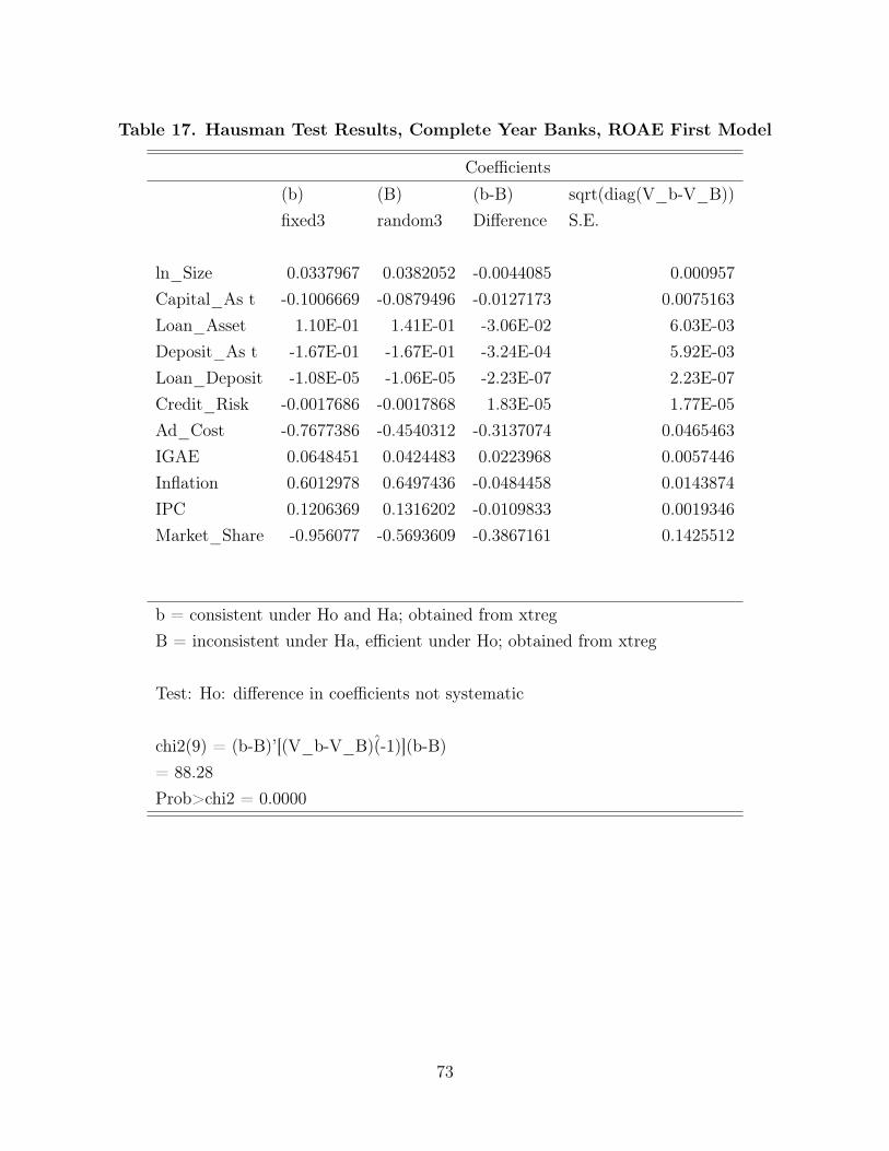
Table 17. Hausman Test Results, Complete Year Banks, ROAE First Model

Coefficients(b) (B) (b-B) sqrt(diag(V_b-V_B))fixed3 random3 Difference S.E.

ln_Size 0.0337967 0.0382052 -0.0044085 0.000957Capital_As t -0.1006669 -0.0879496 -0.0127173 0.0075163Loan_Asset 1.10E-01 1.41E-01 -3.06E-02 6.03E-03Deposit_As t -1.67E-01 -1.67E-01 -3.24E-04 5.92E-03Loan_Deposit -1.08E-05 -1.06E-05 -2.23E-07 2.23E-07Credit_Risk -0.0017686 -0.0017868 1.83E-05 1.77E-05Ad_Cost -0.7677386 -0.4540312 -0.3137074 0.0465463IGAE 0.0648451 0.0424483 0.0223968 0.0057446Inflation 0.6012978 0.6497436 -0.0484458 0.0143874IPC 0.1206369 0.1316202 -0.0109833 0.0019346Market_Share -0.956077 -0.5693609 -0.3867161 0.1425512

b = consistent under Ho and Ha; obtained from xtregB = inconsistent under Ha, efficient under Ho; obtained from xtreg

Test: Ho: difference in coefficients not systematic

chi2(9) = (b-B)’[(V_b-V_B)(̂-1)](b-B)= 88.28Prob>chi2 = 0.0000

73

Table 18. Hausman Test Results, Complete Year Banks, ROAE SecondModel

Coefficients(b) (B) (b-B) sqrt(diag(V_b-V_B))fixed4 random4 Difference S.E.

ln_Size 0.0340816 0.0368435 -0.0027619 0.0007564Capital_As t -0.0384788 -0.0264679 -0.0120109 0.0057671Loan_Deposit -8.69E-06 -8.73E-06 3.96E-08 1.53E-07Credit_Risk -1.28E-03 -1.27E-03 -1.56E-05 1.34E-05Ad_Cost -8.00E-01 -6.09E-01 -1.91E-01 3.84E-02IGAE 0.0752477 0.0632645 1.20E-02 4.35E-03Inflation 0.6148322 0.6509946 -0.0361624 0.011931IPC 0.1247806 0.1299688 -0.0051881 0.0013204Market_Share -0.9131129 -0.6682897 -0.2448232 0.1259541

b = consistent under Ho and Ha; obtained from xtregB = inconsistent under Ha, efficient under Ho; obtained from xtreg

Test: Ho: difference in coefficients not systematic

chi2(7) = (b-B)’[(V_b-V_B)(̂-1)](b-B)= 32.48Prob>chi2 = 0.0000

Table 19. Wooldridge Test For Autocorrelation, Six Year Banks, ROAAFirst Model

Wooldridge test for autocorrelation in panel dataH0: no first-order autocorrelationF( 1, 42) = 110.269Prob > F = 0.0000

74

Table 20. Wooldridge Test For Autocorrelation, Six Year Banks, ROAASecond Model

Wooldridge test for autocorrelation in panel dataH0: no first-order autocorrelationF( 1, 42) = 110.272Prob > F = 0.0000

Table 21. Wooldridge Test For Autocorrelation, Six Year Banks, ROAEFirst Model

Wooldridge test for autocorrelation in panel dataH0: no first-order autocorrelationF( 1, 42) = 237.784Prob > F = 0.0000

Table 22. Wooldridge Test For Autocorrelation, Six Year Banks, ROAESecond Model

Wooldridge test for autocorrelation in panel dataH0: no first-order autocorrelationF( 1, 42) = 235.452Prob > F = 0.0000

Table 23. Wooldridge Test For Autocorrelation, Ten Year Banks, ROAAFirst Model

Wooldridge test for autocorrelation in panel dataH0: no first-order autocorrelationF( 1, 35) = 72.930Prob > F = 0.0000

75

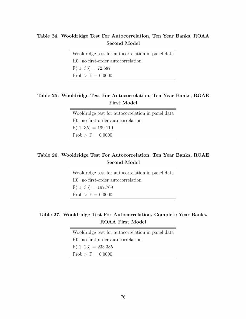
Table 24. Wooldridge Test For Autocorrelation, Ten Year Banks, ROAASecond Model

Wooldridge test for autocorrelation in panel dataH0: no first-order autocorrelationF( 1, 35) = 72.687Prob > F = 0.0000

Table 25. Wooldridge Test For Autocorrelation, Ten Year Banks, ROAEFirst Model

Wooldridge test for autocorrelation in panel dataH0: no first-order autocorrelationF( 1, 35) = 199.119Prob > F = 0.0000

Table 26. Wooldridge Test For Autocorrelation, Ten Year Banks, ROAESecond Model

Wooldridge test for autocorrelation in panel dataH0: no first-order autocorrelationF( 1, 35) = 197.769Prob > F = 0.0000

Table 27. Wooldridge Test For Autocorrelation, Complete Year Banks,ROAA First Model

Wooldridge test for autocorrelation in panel dataH0: no first-order autocorrelationF( 1, 23) = 233.385Prob > F = 0.0000

76

Table 28. Wooldridge Test For Autocorrelation, Complete Year Banks,ROAA Second Model

Wooldridge test for autocorrelation in panel dataH0: no first-order autocorrelationF( 1, 23) = 248.387Prob > F = 0.0000

Table 29. Wooldridge Test For Autocorrelation, Complete Year Banks,ROAE First Model

Wooldridge test for autocorrelation in panel dataH0: no first-order autocorrelationF( 1, 23) = 40.802Prob > F = 0.0000

Table 30. Wooldridge Test For Autocorrelation, Complete Year Banks,ROAE Second Model

Wooldridge test for autocorrelation in panel dataH0: no first-order autocorrelationF( 1, 23) = 42.314Prob > F = 0.0000

Table 31. Wald Test For Heteroskedasticity, Six Year Banks, ROAA FirstModel

Modified Wald test for groupwise heteroskedasticityin fixed effect regression model

H0: sigma(i)2̂ = sigma2̂ for all i

chi2 (43) = 2.8e+06Prob>chi2 = 0.0000

77

Table 32. Wald Test For Heteroskedasticity, Six Year Banks, ROAA SecondModel

Modified Wald test for groupwise heteroskedasticityin fixed effect regression model

H0: sigma(i)2̂ = sigma2̂ for all i

chi2 (43) = 2.6e+06Prob>chi2 = 0.0000

Table 33. Wald Test For Heteroskedasticity, Six Year Banks, ROAE FirstModel

Modified Wald test for groupwise heteroskedasticityin fixed effect regression model

H0: sigma(i)2̂ = sigma2̂ for all i

chi2 (43) = 61329.28Prob>chi2 = 0.0000

Table 34. Wald Test For Heteroskedasticity, Six Year Banks, ROAE SecondModel

Modified Wald test for groupwise heteroskedasticityin fixed effect regression model

H0: sigma(i)2̂ = sigma2̂ for all i

chi2 (43) = 94121.56Prob>chi2 = 0.0000

78

Table 35. Wald Test For Heteroskedasticity, Ten Year Banks, ROAA FirstModel

Modified Wald test for groupwise heteroskedasticityin fixed effect regression model

H0: sigma(i)2̂ = sigma2̂ for all i

chi2 (36) = 1.5e+06Prob>chi2 = 0.0000

Table 36. Wald Test For Heteroskedasticity, Ten Year Banks, ROAA SecondModel

Modified Wald test for groupwise heteroskedasticityin fixed effect regression model

H0: sigma(i)2̂ = sigma2̂ for all i

chi2 (36) = 1.3e+06Prob>chi2 = 0.0000

Table 37. Wald Test For Heteroskedasticity, Ten Year Banks, ROAE FirstModel

Modified Wald test for groupwise heteroskedasticityin fixed effect regression model

H0: sigma(i)2̂ = sigma2̂ for all i

chi2 (36) = 50218.30Prob>chi2 = 0.0000

79

Table 38. Wald Test For Heteroskedasticity, Ten Year Banks, ROAE SecondModel

Modified Wald test for groupwise heteroskedasticityin fixed effect regression model

H0: sigma(i)2̂ = sigma2̂ for all i

chi2 (36) = 52504.97Prob>chi2 = 0.0000

Table 39. Wald Test For Heteroskedasticity, Complete Year Banks, ROAAFirst Model

Modified Wald test for groupwise heteroskedasticityin fixed effect regression model

H0: sigma(i)2̂ = sigma2̂ for all i

chi2 (24) = 1.8e+05Prob>chi2 = 0.0000

Table 40. Wald Test For Heteroskedasticity, Complete Year Banks, ROAASecond Model

Modified Wald test for groupwise heteroskedasticityin fixed effect regression model

H0: sigma(i)2̂ = sigma2̂ for all i

chi2 (24) = 2.0e+05Prob>chi2 = 0.0000

80

Table 41. Wald Test For Heteroskedasticity, Complete Year Banks, ROAEFirst Model

Modified Wald test for groupwise heteroskedasticityin fixed effect regression model

H0: sigma(i)2̂ = sigma2̂ for all i

chi2 (24) = 66308.83Prob>chi2 = 0.0000

Table 42. Wald Test For Heteroskedasticity, Complete Year Banks, ROAESecond Model

Modified Wald test for groupwise heteroskedasticityin fixed effect regression model

H0: sigma(i)2̂ = sigma2̂ for all i

chi2 (24) = 81210.90Prob>chi2 = 0.0000

81

Table 43. Fixed Effects Regression, Period: 2001-2006, Before FinancialCrisis, Complete Year Banks

(1) (2) (3) (4)ROAA ROAA ROAE ROAE

ln_Size 0.00134 0.00277 0.0870*** 0.111***(0.00179) (0.00175) (0.0233) (0.0228)

Capital_Asset 0.0868*** 0.0955*** 0.970*** 1.118***(0.00823) (0.00786) (0.107) (0.102)

Loan_Asset 0.00948** 0.151***(0.00444) (0.0576)

Deposit_Asset -0.0195*** -0.325***(0.00426) (0.0552)

Loan_Deposit 0.000000854** 0.00000123*** 0.0000172*** 0.0000233***(0.000000384) (0.000000377) (0.00000498) (0.00000492)

Credit_Risk 0.108*** 0.109*** 1.023*** 1.039***(0.00699) (0.00695) (0.0907) (0.0905)

Ad_Cost -0.532*** -0.534*** -3.594*** -3.626***(0.0266) (0.0265) (0.345) (0.345)

IGAE 0.00669 0.00461 0.437 0.399(0.0240) (0.0241) (0.311) (0.315)

Inflation 0.134** 0.153** 2.611*** 2.929***(0.0672) (0.0676) (0.872) (0.881)

IPC 0.0108*** 0.0104*** 0.128*** 0.121***(0.00233) (0.00234) (0.0302) (0.0306)

Market_Share -0.114*** -0.120*** -2.430*** -2.540***(0.0343) (0.0345) (0.444) (0.449)

_cons 0.0181 -0.00190 -0.633** -0.974***(0.0205) (0.0194) (0.266) (0.253)

N 1286 1286 1286 1286R2 0.549 0.541 0.412 0.396adj. R2 0.537 0.530 0.397 0.381F 138.4 164.3 79.89 91.41p 0 0 1.03e-280 1.11e-295

Standard errors in parentheses

* p<0.10, ** p<0.05, *** p<0.010

82

Table 44. Fixed Effects Regression, Period: 2007-2009, During FinancialCrisis, Complete Year Banks

(1) (2) (3) (4)ROAA ROAA ROAE ROAE

ln_Size -0.00175 -0.00229* 0.0222 0.0129(0.00145) (0.00135) (0.0139) (0.0130)

Capital_Asset 0.0162* 0.0167** -0.0999 -0.111(0.00853) (0.00838) (0.0819) (0.0805)

Loan_Asset -0.00371 0.0218(0.00591) (0.0567)

Deposit_Asset 0.00828 0.0451(0.00593) (0.0570)

Loan_Deposit -0.00136 -0.00303** -0.00982 -0.0147(0.00193) (0.00129) (0.0186) (0.0124)

Credit_Risk -0.00599 0.00187 -0.537*** -0.433***(0.0137) (0.0126) (0.132) (0.121)

Ad_Cost 0.283*** 0.286*** 4.329*** 4.353***(0.0246) (0.0245) (0.236) (0.236)

IGAE 0.0319*** 0.0300*** 0.550*** 0.528***(0.00678) (0.00668) (0.0651) (0.0642)

Inflation -0.137*** -0.133*** -0.546 -0.539(0.0477) (0.0476) (0.458) (0.458)

IPC 0.00138 0.00117 0.0430*** 0.0385***(0.00136) (0.00133) (0.0131) (0.0128)

Market_Share 0.0837*** 0.0798*** 0.707** 0.659**(0.0305) (0.0304) (0.293) (0.292)

_cons 0.0199 0.0295* -0.330** -0.190(0.0175) (0.0158) (0.168) (0.152)

N 792 792 792 792R2 0.250 0.247 0.516 0.513adj. R2 0.218 0.217 0.495 0.494F 22.94 27.72 73.45 89.15p 3.73e-90 2.20e-101 2.91e-208 5.08e-226

Standard errors in parentheses

* p<0.10, ** p<0.05, *** p<0.010

83

Table 45. Fixed Effects Regression, Period: 2010-2019, After FinancialCrisis, Complete Year Banks

(1) (2) (3) (4)ROAA ROAA ROAE ROAE

ln_Size 0.00589*** 0.00661*** 0.0221*** 0.0217***(0.000642) (0.000639) (0.00443) (0.00441)

Capital_Asset 0.0761*** 0.0840*** 0.150*** 0.179***(0.00569) (0.00571) (0.0393) (0.0394)

Loan_Asset 0.0101*** -0.0485***(0.00271) (0.0187)

Deposit_Asset -0.0223*** -0.112***(0.00236) (0.0163)

Loan_Deposit 0.0000133 0.0000262 -0.000151 -0.000120(0.0000217) (0.0000219) (0.000150) (0.000151)

Credit_Risk -0.000112*** -0.0000680*** -0.000997*** -0.000906***(0.0000259) (0.0000257) (0.000179) (0.000177)

Ad_Cost -0.0534*** -0.0342*** -0.0251 -0.0466(0.00977) (0.00922) (0.0675) (0.0636)

IGAE 0.0576*** 0.0733*** 0.362*** 0.554***(0.0154) (0.0153) (0.106) (0.105)

Inflation -0.00782 -0.0228 0.385*** 0.245**(0.0165) (0.0166) (0.114) (0.115)

IPC 0.00419*** 0.00559*** 0.00550 0.0166(0.00147) (0.00148) (0.0102) (0.0102)

Market_Share -0.0812*** -0.0639*** -0.263 -0.00197(0.0237) (0.0236) (0.164) (0.163)

_cons -0.0557*** -0.0720*** -0.115** -0.192***(0.00770) (0.00763) (0.0532) (0.0526)

N 2746 2746 2746 2746R2 0.124 0.095 0.060 0.031adj. R2 0.113 0.084 0.049 0.020F 34.76 31.50 15.83 9.638p 3.57e-185 2.04e-160 6.06e-83 4.50e-44

Standard errors in parentheses

* p<0.10, ** p<0.05, *** p<0.010

84

Table 46. Time Fixed Effects Regression, Period: 2001-2006, BeforeFinancial Crisis, Complete Year Banks

(1) (2) (3) (4)ROAA ROAA ROAE ROAE

ln_Size 0.00230 0.00450** 0.118*** 0.153***(0.00217) (0.00206) (0.0280) (0.0267)

Capital_Asset 0.0910*** 0.102*** 1.110*** 1.289***(0.00947) (0.00880) (0.122) (0.114)

Loan_Asset 0.00814* 0.125**(0.00462) (0.0596)

Deposit_Asset -0.0174*** -0.278***(0.00453) (0.0584)

Loan_Deposit 0.000000917** 0.00000126*** 0.0000177*** 0.0000231***(0.000000399) (0.000000391) (0.00000515) (0.00000506)

Credit_Risk 0.108*** 0.109*** 1.005*** 1.016***(0.00726) (0.00719) (0.0937) (0.0931)

Ad_Cost -0.527*** -0.523*** -3.458*** -3.390***(0.0280) (0.0277) (0.361) (0.359)

IGAE 0 0 0 0(.) (.) (.) (.)

Inflation 0 0 0 0(.) (.) (.) (.)

IPC 0.0121* 0.0132** 0.152* 0.170**(0.00625) (0.00628) (0.0807) (0.0813)

Market_Share -0.122*** -0.134*** -2.701*** -2.888***(0.0355) (0.0355) (0.458) (0.460)

_cons 0.0133 -0.0143 -0.852*** -1.299***(0.0234) (0.0215) (0.302) (0.278)

N 1286 1286 1286 1286R2 0.556 0.551 0.428 0.417adj. R2 0.523 0.518 0.384 0.374F 22.02 22.22 13.12 12.96p 5.32e-195 4.80e-194 5.62e-124 1.02e-120

Standard errors in parentheses

* p<0.10, ** p<0.05, *** p<0.010

85

Table 47. Time Fixed Effects Regression, Period: 2007-2009, DuringFinancial Crisis, Complete Year Banks

(1) (2) (3) (4)ROAA ROAA ROAE ROAE

ln_Size 0.00242 0.000106 0.0810*** 0.0519***(0.00158) (0.00144) (0.0148) (0.0136)

Capital_Asset 0.0347*** 0.0302*** 0.161* 0.0880(0.00894) (0.00873) (0.0838) (0.0822)

Loan_Asset 0.00263 0.106*(0.00598) (0.0561)

Deposit_Asset 0.0115* 0.0603(0.00600) (0.0562)

Loan_Deposit -0.00306 -0.00430*** -0.0368** -0.0323***(0.00195) (0.00132) (0.0183) (0.0125)

Credit_Risk -0.0321** -0.00802 -0.866*** -0.594***(0.0141) (0.0127) (0.133) (0.120)

Ad_Cost 0.301*** 0.302*** 4.582*** 4.590***(0.0245) (0.0247) (0.230) (0.232)

IGAE 0 0 0 0(.) (.) (.) (.)

Inflation 0 0 0 0(.) (.) (.) (.)

IPC 0.0101*** 0.00835*** 0.133*** 0.112***(0.00213) (0.00210) (0.0200) (0.0197)

Market_Share 0.0789*** 0.0692** 0.541* 0.444(0.0303) (0.0304) (0.284) (0.287)

_cons -0.0381** -0.00401 -1.053*** -0.650***(0.0187) (0.0163) (0.175) (0.154)

N 792 792 792 792R2 0.302 0.288 0.570 0.557adj. R2 0.240 0.227 0.532 0.520F 7.300 7.190 22.42 22.40p 1.30e-45 7.42e-44 3.06e-132 4.80e-130

Standard errors in parentheses

* p<0.10, ** p<0.05, *** p<0.010

86

Table 48. Time Fixed Effects Regression, Period: 2010-2019, After FinancialCrisis, Complete Year Banks

(1) (2) (3) (4)ROAA ROAA ROAE ROAE

ln_Size 0.0126*** 0.0136*** 0.0560*** 0.0673***(0.000947) (0.000925) (0.00652) (0.00634)

Capital_Asset 0.0953*** 0.103*** 0.255*** 0.307***(0.00609) (0.00605) (0.0419) (0.0415)

Loan_Asset 0.0171*** -0.00984(0.00282) (0.0195)

Deposit_Asset -0.0180*** -0.102***(0.00245) (0.0169)

Loan_Deposit 0.0000594*** 0.0000739*** 0.0000660 0.000178(0.0000222) (0.0000224) (0.000153) (0.000153)

Credit_Risk -0.000122*** -0.0000709*** -0.00114*** -0.00100***(0.0000264) (0.0000260) (0.000182) (0.000178)

Ad_Cost -0.0556*** -0.0295*** -0.0485 -0.0238(0.00982) (0.00924) (0.0677) (0.0633)

IGAE 0 0 0 0(.) (.) (.) (.)

Inflation 0 0 0 0(.) (.) (.) (.)

IPC 0.0150*** 0.0160*** 0.0614** 0.0898***(0.00369) (0.00367) (0.0254) (0.0251)

Market_Share -0.124*** -0.127*** -0.484*** -0.400**(0.0241) (0.0243) (0.166) (0.167)

_cons -0.138*** -0.153*** -0.505*** -0.700***(0.0117) (0.0110) (0.0808) (0.0755)

N 2746 2746 2746 2746R2 0.166 0.144 0.111 0.096adj. R2 0.118 0.096 0.060 0.044F 4.075 3.509 2.556 2.206p 2.70e-49 1.10e-37 2.72e-20 3.08e-14

Standard errors in parentheses

* p<0.10, ** p<0.05, *** p<0.010

87

List of Tables

5.1 Descriptive Statistics, Six Year Banks . . . . . . . . . . . . . . . . . . . . 185.2 Descriptive Statistics, Ten Year Banks . . . . . . . . . . . . . . . . . . . 185.3 Descriptive Statistics, Complete Year Banks . . . . . . . . . . . . . . . . 195.4 Correlation Matrix, Six Year Banks . . . . . . . . . . . . . . . . . . . . . 215.5 Correlation Matrix, Ten Year Banks . . . . . . . . . . . . . . . . . . . . . 225.6 Correlation Matrix, Complete Year Banks . . . . . . . . . . . . . . . . . 23

6.1 Six Year Banks, Period of Regression: 2007-2019 . . . . . . . . . . . . . . 286.2 Ten Year Banks, Period of Regression: 2007-2019 . . . . . . . . . . . . . 286.3 Complete Year Banks, Period of Regression: 2001-2019 . . . . . . . . . . 28

7.1 Fixed Effects Regression, Period: 2007-2019, Clusters, Six Year Banks . . 367.2 Fixed Effects Regression, Period: 2007-2019, Clusters, Ten Year Banks . 377.3 Fixed Effects Regression, Period: 2001-2019, Clusters, Complete Year Banks 387.4 Time Fixed Effects Regression, Period: 2007-2019, Clusters, Six Year Banks 397.5 Time Fixed Effects Regression, Period: 2007-2019, Clusters, Ten Year Banks 407.6 Time Fixed Effects Regression, Period: 2001-2019, Clusters, Complete

Year Banks . . . . . . . . . . . . . . . . . . . . . . . . . . . . . . . . . . 417.7 Fixed Effects Regression, Period: 2001-2006, Before Financial Crisis,

Clusters, Complete Year Banks . . . . . . . . . . . . . . . . . . . . . . . 447.8 Fixed Effects Regression, Period: 2007-2009, During Financial Crisis,

Clusters, Complete Year Banks . . . . . . . . . . . . . . . . . . . . . . . 457.9 Fixed Effects Regression, Period: 2010-2019, After Financial Crisis,

Clusters, Complete Year Banks . . . . . . . . . . . . . . . . . . . . . . . 467.10 Time Fixed Effects Regression, Period: 2001-2006, Before Financial Crisis,

Clusters, Complete Year Banks . . . . . . . . . . . . . . . . . . . . . . . 477.11 Time Fixed Effects Regression, Period: 2007-2009, During Financial Crisis,

Clusters, Complete Year Banks . . . . . . . . . . . . . . . . . . . . . . . 48

88

7.12 Time Fixed Effects Regression, Period: 2010-2019, After Financial Crisis,Clusters, Complete Year Banks . . . . . . . . . . . . . . . . . . . . . . . 49

1 Fixed Effects Regression, Period: 2007-2019, Six Year Banks . . . . . . . 572 Fixed Effects Regression, Period: 2007-2019, Ten Year Banks . . . . . . . 583 Fixed Effects Regression, Period: 2001-2019, Complete Year Banks . . . 594 Time Fixed Effects Regression, Period: 2007-2019, Six Year Banks . . . . 605 Time Fixed Effects Regression, Period: 2007-2019, Ten Year Banks . . . 616 Time Fixed Effects Regression, Period: 2001-2019, Complete Year Banks 627 Hausman Test Results, Six Year Banks, ROAA First Model . . . . . . . 638 Hausman Test Results, Six Year Banks, ROAA Second Model . . . . . . 649 Hausman Test Results, Six Year Banks, ROAE First Model . . . . . . . . 6510 Hausman Test Results, Six Year Banks, ROAE Second Model . . . . . . 6611 Hausman Test Results, Ten Year Banks, ROAA First Model . . . . . . . 6712 Hausman Test Results, Ten Year Banks, ROAA Second Model . . . . . . 6813 Hausman Test Results, Ten Year Banks, ROAE First Model . . . . . . . 6914 Hausman Test Results, Ten Year Banks, ROAE Second Model . . . . . . 7015 Hausman Test Results, Complete Year Banks, ROAA First Model . . . . 7116 Hausman Test Results, Complete Year Banks, ROAA Second Model . . . 7217 Hausman Test Results, Complete Year Banks, ROAE First Model . . . . 7318 Hausman Test Results, Complete Year Banks, ROAE Second Model . . . 7419 Wooldridge Test For Autocorrelation, Six Year Banks, ROAA First Model 7420 Wooldridge Test For Autocorrelation, Six Year Banks, ROAA Second Model 7521 Wooldridge Test For Autocorrelation, Six Year Banks, ROAE First Model 7522 Wooldridge Test For Autocorrelation, Six Year Banks, ROAE Second Model 7523 Wooldridge Test For Autocorrelation, Ten Year Banks, ROAA First Model 7524 Wooldridge Test For Autocorrelation, Ten Year Banks, ROAA Second Model 7625 Wooldridge Test For Autocorrelation, Ten Year Banks, ROAE First Model 7626 Wooldridge Test For Autocorrelation, Ten Year Banks, ROAE Second Model 7627 Wooldridge Test For Autocorrelation, Complete Year Banks, ROAA First

Model . . . . . . . . . . . . . . . . . . . . . . . . . . . . . . . . . . . . . 7628 Wooldridge Test For Autocorrelation, Complete Year Banks, ROAA

Second Model . . . . . . . . . . . . . . . . . . . . . . . . . . . . . . . . . 7729 Wooldridge Test For Autocorrelation, Complete Year Banks, ROAE First

Model . . . . . . . . . . . . . . . . . . . . . . . . . . . . . . . . . . . . . 77

89

30 Wooldridge Test For Autocorrelation, Complete Year Banks, ROAESecond Model . . . . . . . . . . . . . . . . . . . . . . . . . . . . . . . . . 77

31 Wald Test For Heteroskedasticity, Six Year Banks, ROAA First Model . . 7732 Wald Test For Heteroskedasticity, Six Year Banks, ROAA Second Model 7833 Wald Test For Heteroskedasticity, Six Year Banks, ROAE First Model . . 7834 Wald Test For Heteroskedasticity, Six Year Banks, ROAE Second Model 7835 Wald Test For Heteroskedasticity, Ten Year Banks, ROAA First Model . 7936 Wald Test For Heteroskedasticity, Ten Year Banks, ROAA Second Model 7937 Wald Test For Heteroskedasticity, Ten Year Banks, ROAE First Model . 7938 Wald Test For Heteroskedasticity, Ten Year Banks, ROAE Second Model 8039 Wald Test For Heteroskedasticity, Complete Year Banks, ROAA First Model 8040 Wald Test For Heteroskedasticity, Complete Year Banks, ROAA Second

Model . . . . . . . . . . . . . . . . . . . . . . . . . . . . . . . . . . . . . 8041 Wald Test For Heteroskedasticity, Complete Year Banks, ROAE First Model 8142 Wald Test For Heteroskedasticity, Complete Year Banks, ROAE Second

Model . . . . . . . . . . . . . . . . . . . . . . . . . . . . . . . . . . . . . 8143 Fixed Effects Regression, Period: 2001-2006, Before Financial Crisis,

Complete Year Banks . . . . . . . . . . . . . . . . . . . . . . . . . . . . . 8244 Fixed Effects Regression, Period: 2007-2009, During Financial Crisis,

Complete Year Banks . . . . . . . . . . . . . . . . . . . . . . . . . . . . . 8345 Fixed Effects Regression, Period: 2010-2019, After Financial Crisis,

Complete Year Banks . . . . . . . . . . . . . . . . . . . . . . . . . . . . . 8446 Time Fixed Effects Regression, Period: 2001-2006, Before Financial Crisis,

Complete Year Banks . . . . . . . . . . . . . . . . . . . . . . . . . . . . . 8547 Time Fixed Effects Regression, Period: 2007-2009, During Financial Crisis,

Complete Year Banks . . . . . . . . . . . . . . . . . . . . . . . . . . . . . 8648 Time Fixed Effects Regression, Period: 2010-2019, After Financial Crisis,

Complete Year Banks . . . . . . . . . . . . . . . . . . . . . . . . . . . . . 87

90