1

ITQ’s in Chile: Measuring the Economic Benefits of Reform†

Andrés Gómez-Loboa

Julio Peña-Torresb

and

Patricio Barríac

(March 2nd, 2007) Abstract In 2001 an individual (operationally transferable) quota system was introduced for all the most important industrial fisheries in Chile. This system was put in place after years of declining stocks and over investment. In this paper we describe this reform and estimate related allocative efficiency benefits for the most important industrial fishery in the country, the southern pelagic fishery. Benefits were estimated using a bioeconomic model and Monte Carlo techniques. This approach allows benefits to be estimated using more realistic counterfactual scenarios than just comparing the fishery before and after the reform. Estimated discounted net benefits reach US$123 to US$366 million in the period 2001 to 2020. Fleet size fell from 148 active boats in 2000 to 65 in 2002 as a direct consequence of the reform. Among the interesting features of the recent Chilean experience is the way the political economy of the reform was facilitated by the prior introduction of de facto individual quotas within the framework of fishery research activities. When the authorities closed the southern pelagic fishery because of biological problems between 1997 and 2000, they organized ‘experimental’ fishing expeditions in which participant boats were given the right to fish a certain amount of resources per expedition. This pseudo quota system allowed fishermen to experience directly the benefits of individual quotas and that was instrumental to the political agreement leading to the reform. This successful gradual approach may be of interest to other countries planning to introduce individual quotas. Finally, it is important to note that the Chilean southern industrial pelagic fishery has average catches of over 1.4 million tons a year, making it one of the largest fisheries in the world to be regulated by individual quotas.

JEL Classification: Q22

Keywords: Bioeconomic model, pelagic fisheries, individual transferable quotas

† We thank Constanza Hill for her able research assistance in this paper. We gratefully acknowledge the financial support from the Fondo Nacional de Desarrollo Científico y Tecnológico (FONDECYT project Nº1020765). We are also grateful to Institute for the Development of Fisheries (IFOP) for making the data available. a Department of Economics, University of Chile, Santiago, Chile (agomezlo@econ.uchile.cl). b Department of Economics, University Alberto Hurtado, ILADES-Georgetown University, Santiago, Chile (jpena@uahurtado.cl). c Fisheries Development Institute, Valparaíso, Chile. (pbarria@ifop.cl)

2

1. Introduction

The fishing industry is one of the most important sectors of the Chilean economy. Yearly landings

of fish averaged 5.4 million tons between 1993 and 2003 and exports of products directly related to

the fishing industry, including fish meal and salmons from aquaculture, reached US$1.847 million

in 2003, accounting for close to 10% of total exports that year.1

Until very recently the management of fisheries in Chile was for the most part based on the use of a

yearly global quota (TAC), effort restrictions (licenses) and seasonal closure of fisheries justified on

biological considerations. However, in 1991, during the debates surrounding the writing of a new

fisheries law, there was much discussion of introducing an individual transferable quota (ITQ)

system to avoid the emerging problems of ‘racing’, over investment, effort distortions, and

declining length of fishing seasons.

At the time it became political impossible to introduce ITQ’s due to the opposition of an important

industrial group that was changing the focus of its activities from the north of the country to the

south.2 During the 1980’s the most important fishery was the northern pelagic fishery (see Figure

1), based on the Anchovy (Engraulis ringens) and Spanish Sardine (Sardinops sagax), used in the

production of fishmeal. Industrial catches of Spanish Sardine peaked in 1985 with 2.6 million tons

(Barria y Serra, 1989). However, by the end of the eighties it was clear that this fishery was

collapsing (landings reached 1.4 million tons by 1989 and have only averaged 123 thousand tons

during the last ten years; Sernapesca, 2003). The center of gravity of the industry was now turning

towards the southern pelagic fishery based on Jack Maquerel (Trachurus murphyi). The strategy of

the industrial group owning the fleet and processing plants in the north was to migrate south and

enter the emerging southern pelagic fishery. An ITQ system would have made this migration much

more costly, if not impossible, since its introduction would have required some type of

granfathering in the allocation of initial quotas which would have forced newcomers without history

in the fishery to pay to enter this fishery. Therefore, the industrial group of the north lobbied hard

against an ITQ system, and won.

1 Fish landing data is from Sernapesca (2003). Export data was constructed by authors based on information from the Central Bank of Chile. 2 However, the 1991 fisheries law did introduce ITQ’s for some minor fisheries that were closed due to previous over fishing. In the case of these fisheries, quotas were not allocated by historical rights but were actually tendered to the highest price bidder (Peña-Torres, 1997, 2002).

3

Figure 1: Chilean Pelagic Fisheries

(A): Northern Fishery (B): Southern Fishery

During the nineties the southern pelagic fishery flourished. Although the number of licenses and

storage capacity in this fishery was formally fixed in 1991, fishing boats and capacity kept

increasing through a series of loopholes in the regulations.3 Potential fishing effort, measured by

storage capacity of the fleet, grew 134% between 1989 and 1995. Landings steadily increased

during this period, reaching a peak of 4 million tons in 1995.

By the late nineties, it was evident that the southern fishery was in problems. The decline of stocks

due to over fishing, together with a strong ‘El Niño’ phenomenon in 1997-1998, reduced the adult

biomass considerably, and landings began to show an above average presence of juveniles. Storage

capacity had kept increasing making over investment in the fishery acute.

As a reaction to the increasing presence of juveniles in catches, the authorities closed the fishery

starting in December 1997. However, the social and political impacts of a complete closure would

have been enormous. Instead, the authorities devised a mechanism so that the fleet could continue

to operate but in a controlled and orderly fashion that would not jeopardize the sustainability of the

3 For example, by licensing new boats in the Xth region, the southernmost part of the fishery.

4

fishery. To this end, a series of ‘research’ or ‘experimental’ fishing expeditions were organized in

the following three years. Participant boats had to sweep a pre-determined stretch of sea and locate

existing schools of fish. This information was used by the authorities to gauge with more precision

the level of biomass and its distribution. Once this was over, participant boats had the right to

capture a pre-allocated per vessel quota of fish.

These controlled fishing expeditions, besides reducing the effort exerted on the resource, operated

in practice as a pseudo individual quota system that served to show companies the benefits of such a

system. Compared to the previous ‘Olympic race’ for resources, the individual quotas assigned to

participant ships during the ‘experimental’ fishing expeditions allowed fishermen to optimize the

use of their fleet.4

By the year 2000 there was consensus among industry participants, and the authorities, that in order

to lift the closure of the fishery, an individual quota system would have to be introduced. The

stumbling block for such a reform was the difficulty in reaching an agreement on the initial

allocation of quotas.5 An agreement was reached in the end and individual quotas were introduced

for the most important industrial fisheries in Chile. They became operational in February 2001 and

were initially given for a 2-year duration period. In 2002, a further reform extended these rights for

10 more years and incorporated the northern pelagic fisheries as well.

The effects of this quota system were instantaneous. The reform explicitly facilitated the merger of

fishing operations of fleets from different companies, a sort of ‘operational transferability’ of

quotas. Very soon after the reform, the number of boats in operation was reduced drastically from

148 in 2000 to 65 in 2002. Also, only the largest (from 500 to 1900 cubic meters of storage

capacity) and newest boasts were kept active. Therefore, the excess capacity of the fleet was soon

corrected, generating direct economic benefits in the form of lower operating costs. Another benefit

of the reform was that due to the elimination of ‘racing for fish’, fishermen can now concentrate on

catching less per trip, improving the quality of fish landings. This enabled the industry to allocate a

higher percentage of landings to the higher value-added human consumption segment of the market,

rather than to fishmeal production.

4 However, fishermen did not have total freedom to decide their fishing effort’s technological composition. During these years, the fishery regulator prioritized the allocation of fishing quotas to the relatively bigger industrial vessels which were previously operating in this fishery. 5 To be politically acceptable grand fathering of rights was inevitable. However, the strategy followed by the authorities was to extract some of the rents generated in the fishery through an increase in the annual licensing fee. For more details on this, see Peña-Torres (2002a,b).

5

In this paper, we describe the ITQ system introduced in Chile and offer a preliminary estimate of its

direct allocative efficiency benefits. To this end we use a bioeconomic model of the Southern Jack

Mackerel fishery to generate a more convincing counterfactual scenario to the reform.

Alternatively, we could have compared the fishery before and after the reform, but it is highly

unlikely that the pre-reform situation would give a good indication of what would have happened

without the reform. Over investment may have worsened, increasing the economic costs of the pre-

reform regulations. Also, the size and stability of the stock may have been more vulnerable in a pre-

reform situation. But most importantly, this fishery is subject to a number of other regulations such

as vessel licensing and a TAC. The benefits of the reform depend on the type and level of these

regulations adopted for the future. The correct way then to measure the benefits of the reform is to

simulate the future evolution of the fishery under different scenarios and regulatory systems. Thus,

in this paper we use a biological age-structured model for the Jack Mackerel (Trachurus murphyi)

stock, an estimated stock-recruitment function for this resource, several functions determining fleet

dynamics, and a catch function, to model the dynamics of the fishery.

The parameters of these equations were estimated econometrically using data from 1985 to 2002

(from 1975, in the case of the biological equations). The stock-recruitment relationship, the catch

equation and the fleet dynamic equations all have random shocks whose distributions were

estimated from the residuals of each individual equation. We then use Monte Carlo techniques,

taking draws from these random shock distributions, to generate 100 possible future scenarios for

the fishery with and without the reform introduced in 2001. Pair wise comparison of each scenario

with and without the reform generates a distribution of the economic benefits of the introduction of

the ITQ system in this fishery.

The results show that the direct allocative efficiency benefits of the reform are substantial.

Depending on the scenario, the net discounted benefits, using a 10% discount rate over the 2001-

2020 period, are between US$123 and US$366 million.6 These scenarios assume a TAC of 1.1

million tons for the industrial fleet for each year, close to the current level set by the authorities for

the industrial fleet. The results are not very sensitive to the range of TACs assumed in the

simulations.

6 In Chile, social value discounting currently uses a 10% annual rate. The resulting net present values imply yearly net benefit flows of US$14.5 and US$43 million, respectively. Given that along the years 2002-2003 the southern Jack Mackerel industrial fishery exported about US$230 million per year, the estimated net annual benefits of the ITQ reform correspond to about 6.3% - 18.7% of the annually exported value by this fishery.

6

The paper is organized as follows. First we present a detailed description of the southern pelagic

fishery in Chile. We then present a detailed description of the ITQ system introduced in 2001 and

expanded in 2002. Following this we specify the bioeconomic model of the fishery and present the

estimation results for each equation. The Monte Carlo results and the estimated benefits of the

reform are then presented. The paper concludes with a discussion of the policy lessons derived from

the Chilean experience and possible directions for future research in this fishery.

2. The Southern Pelagic Fishery

This fishery runs along the Vth to Xth Regions, from latitude 33ºS to 41ºS, although its main center

of operation is in front of the Talcahuano area in the VIIIº region of the country (L36ºS; see Figure

2), the zone where industrial fishing was first initiated around the mid 1940s. Industrial fishing has

been historically concentrated on pelagic species used primarily for the production of fishmeal.

Although in the early stages of this fishery the main targeted species were the Anchovy (Engraulis

ringens) and Common Sardine (Clupea bentincki), since the early 1980s the Jack Mackerel

increasingly became the dominant species targeted by industrial vessels. Landings of Jack Mackerel

accounted for 82% of the total industrial catch between 1985 and 2002, making it by far the central

resource of this industrial fishery.7 Of the total catch of Jack Mackerel within the Chilean EEZ,

including non-industrial landings as well as industrial catches in other parts of the country, and also

adding the catch caught by international vessels off the Chilean EEZ, the southern pelagic industrial

fleet landed on average 64% of this species between 1985 and 2000. Thus, this fleet is by far the

most important anthropogenic influence on this species.

In the beginning of the eighties this fishery was in a strong development phase both in terms of

fishing capacity and processing capacity (see Table 1). From 1980 to 1985 the number of industrial

vessels more than doubled, while the storage capacity of the fleet more than quadrupled. In the

following decade the storage capacity of the fleet again increased by a factor of four. This coincided

with the introduction of larger vessels (with greater capacity of displacement) in the industrial fleet.8

In terms of the resulting fishing effort, there was an increase of 6.7 times between 1985 and 1995.9

7 This percentage is even higher, 88%, if the average is taken between 1985 and 1997 before the Jack Mackerel fishery was closed. 8 The first ships over 790 m3 of storage capacity initiated operations in this fishery during 1989. In 1995 the number of ships with a storage capacity greater than 790 m3 represented 34% of the industrial fleet. 9 The fishing effort index was constructed using the annual haul of the industrial fleet. That is, the sum over the whole fleet of the storage capacity of each individual ship (in m3) multiplied by the days of fishing operations during each year.

7

Table 1: The Southern Pelagic Industrial Fishery

Fleet Yearly Landings (millions of tons)

Biomass (1,000 of tons)

Year Effort index

(1)

Number of ships

(2)

Storage capacity

(1,000 m3) (3)

3 main Species

(4)

Jack Mackerel

(5)

Aggregate: 3 main Species

(6)

Jack Mackerel (National

Total) (7)

1975 37 4,3 2.232 1980 47 6,3 7.183 1985 100,0 97 28,4 0,953 0,854 15.188 1986 143,6 93 29,9 1,128 1,051 15.899 1987 156,5 93 33,2 1,528 1,341 15.847 1988 191,0 105 40,4 1,705 1,439 15.194 1989 236,4 108 50,5 2,001 1,677 16.084 1990 307,7 145 67,9 2,093 1,860 16.001 15.454 1991 362,9 179 84,4 2,870 2,331 15.598 13.705 1992 424,7 176 87,1 2,882 2,472 12.501 10.857 1993 462,2 171 95,5 2,618 2,392 12.085 10.246 1994 572,3 168 103,9 3,575 3,254 11.157 9.492 1995 674,7 179 117,8 4,021 3,732 9.461 8.033 1996 636,8 159 113,6 3,401 2,805 10.151 7.322 1997 741,9 177 133,3 2,947 2,533 9.845 6.828 1998 610,9 163 131,0 2,079 1,465 10.067 7.085 1999 595,3 161 131,1 2,550 1,082 8.936 6.708 2000 447,3 148 125,9 1,802 1,063 8.928 7.048 2001 310,6 107 102,3 1,548 1,215 10.288 6.611 2002 370,8 65 70,3 1,400 1,142 9.940 6.477 (1) Annual haul (fishing days times storage capacity); index: 1985 = 100. (2) Number of industrial ships operating at least once during each year. (3) Aggregate storage capacity in thousands of cubic meters. (4) Landings of the three main species (Common Sardine, Anchovy and Jack Mackerel). (6) and (7): Average annual biomass (recruits plus higher aged cohorts), (6) for the fishing grounds between the Vth and Xth regions and (7) at the national level. Sources (1)–(7): National Fisheries Research Institute (IFOP).

Total industrial pelagic landings grew uninterrupted until they reached a peak of 3.5 – 4 million

tons in 1994 and 1995.10

From then on catches began to fall, partially coinciding with a very intense ‘El Niño’ phenomenon

beginning in 1997 and lasting until the middle of 1998.11 If we consider the three main species

caught, the level of catches in 2002 were less than half the 1994-95 peak; in the case of the Jack

Mackerel the drop was even greater.

10 Semi-industrial and artisanal fishermen landed another 0.5 million tons of these resources in both years. These fleets operate closer to the coast and capture mainly common sardine and anchovy. 11 This was the ‘El Niño’ of greatest intensity to have occurred during the 20th century. However, the consensus opinion in the fishing sector was that over-fishing during the previous years was much to blame for the falling catches, or at least in making the stock less resilient to oceanographic shocks such as ‘El Niño’.

8

The dynamics just described for the annual catch was preceded by a similar evolution in the

available biomass of the three main species. Columns 6 and 7 of Table 1 present the official

(IFOP’s) estimates of average yearly stock biomass for Jack Mackerel and the aggregate of the three

main species. These estimates include recruits plus all higher aged cohorts. In the case of Jack

Mackerel the estimates are for the total national biomass, while for the two other species it is an

estimate of the stock in the central southern region.12

Beginning in November 1997 there is a reduction in the size and the annual haul of the industrial

fleet in operation in the area. This tendency is related to the closed seasons introduced late in 1997

and that limited the operational capacity of the fleet until the year 2001.

From November 1997 through December 2000 a biological closure was imposed on the Jack

Mackerel fishery. The Anchovy and Sardine fishery had closed seasons from December to January

(recruitment season) and from July to August (reproduction season) each year.

During this period, the only possibility of capturing Jack Mackerel was to participate in one of the

‘research’ fishing expeditions organized by the authorities. Boats that qualified mainly those with

more than 700 cubic meters of storage capacity had to sign a formal agreement with the

authorities. Those that would eventually participate were chosen at random from the list of qualified

boats before each expedition.13

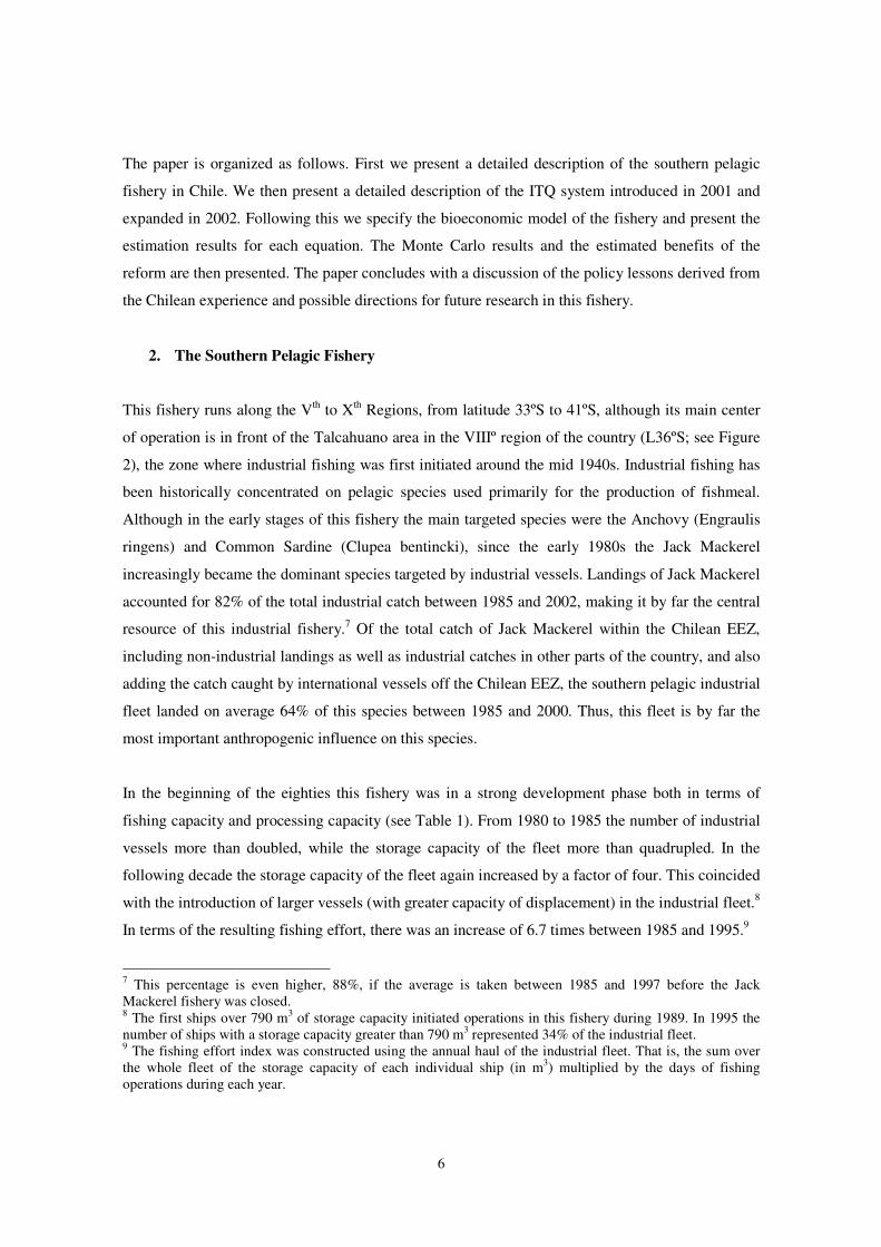
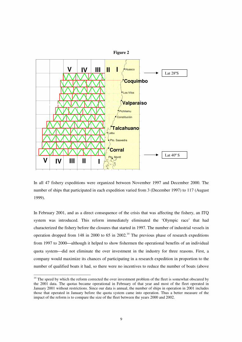
The research fishing expeditions consisted first of a search stage where boats had to follow a pre-

assigned path from the coast outwards in a zig-zag pattern whose length varied from 400 to 500

nautical miles. Each ship had its own course to follow, which differed by 1º latitude from the other

courses. Figure 2 presents an example of the design of an expedition, where the green lines

represent the charted course for each ship. In this stage, ships had to detect schools of Jack

Mackerel, catch some fish and measure some environmental variables in order for the authorities to

better gauge the size and distribution of the resource. Once this stage was completed, ships were

allowed to fish a pre-assigned quota but only within some areas (square areas of between 50 and

100 nautical miles) of their charted course (red squares in Figure 2).

12 Due to the geographic mobility of the Chilean Jack Mackerel stock, its biomass is estimated only at the national level. In contrast, the anchovy and common sardine do have biologically independent regional stocks along the coast of the country. 13 The idea was to ensure that the different participating firms were represented among the chosen vessels.

9

Figure 2

In all 47 fishery expeditions were organized between November 1997 and December 2000. The

number of ships that participated in each expedition varied from 3 (December 1997) to 117 (August

1999).

In February 2001, and as a direct consequence of the crisis that was affecting the fishery, an ITQ

system was introduced. This reform immediately eliminated the ‘Olympic race’ that had

characterized the fishery before the closures that started in 1997. The number of industrial vessels in

operation dropped from 148 in 2000 to 65 in 2002.14 The previous phase of research expeditions

from 1997 to 2000although it helped to show fishermen the operational benefits of an individual

quota systemdid not eliminate the over investment in the industry for three reasons. First, a

company would maximize its chances of participating in a research expedition in proportion to the

number of qualified boats it had, so there were no incentives to reduce the number of boats (above

14 The speed by which the reform corrected the over investment problem of the fleet is somewhat obscured by the 2001 data. The quotas became operational in February of that year and most of the fleet operated in January 2001 without restrictions. Since our data is annual, the number of ships in operation in 2001 includes those that operated in January before the quota system came into operation. Thus a better measure of the impact of the reform is to compare the size of the fleet between the years 2000 and 2002.

84° 82° 80° 78° 76° 74° 72° 70° 43°

41°

39°

37°

35°

33°

31°

29°

27°

L a t i t u d S u r

Huasco

Coquimboo

Los Vilos

Valparaíso Pichilemu

Constitución

Talcahuano Lebu

Pto. Saavedra

Corral Pto. Montt

I. Alejandro Selkirk I. Róbinson

Crusoe

I II III IV V

I II III IV V

Lat 28ºS

Lat 40º S

10

700 cubic meters of storage capacity). Second, boats could still be used in the anchovy and sardine

fishery, especially the smaller ones. Third, there was uncertainty as to the future regulation of the

fishery. In this context, maintaining the whole fleet licensed and operational had an option value for

companies due to the possibility that the fishery would be reopened in the future.

3. The ITQ system implemented in 2001

The individual quota system introduced in February 2001 works as follows. The owners of licensed

ships have a right to a certain percentage of each year’s annual TAC allocated to the industrial

sector for each resource and fishery (expressed in tons).15 The initial allocation rule determining the

(fixed by law) percentage of the TAC for each owner varied slightly among fisheries. There were

two basic rules. In some fisheries the initial percentages were set using a weighted average of the

landings of the ships owned by each company between 1997 to 2000, relative to the total industrial

landings for that period, and the storage capacity of each company’s fleet, relative to the total

storage capacity in each fishery. In order to better explain this rule, let’s define citj, as the landings

of ships owned by company i, in year t of species j. Similarly, define kij, as the storage capacity of

ships owned by company i, in year t.16 Then, the percentage of the industrial TAC of species j

allocated to each company i was defined as:

Ki

Lii qqq ⋅+⋅= 5.05.0

where,

� �

�

= =

==I

i titj

titj

Lij

c

cq

1

2000

1997

2000

1997

15 The annual TAC for each resource is first divided into a TAC for the industrial sector and a TAC for the artisanal sector. Industrial ships are prohibited from operating within the first 5 nautical miles off the coast where the artisanal fleet operates. 16 The storage capacity of each ship was first adjusted to take account of the fact that some ships were only authorized to fish in a sub-region of the fishery.

11

�=

=I

ii

iKij

k

kq

12000

2000

where I is the total number of companies in the industry.

The other initial allocation rule was just based on the landings of the species in the years 1999 and

2000. For these fisheries the percentage of the industrial TAC was defined as:

� �

�

= =

==I

i titj

titj

ij

c

cq

1

2000

1999

2000

1999

.

In the Appendix we present the allocation rule used for each fishery in the country. Here it suffices

to mention that the first allocation rule was used for the three species relevant for the southern

pelagic fishery.

Quotas were initially set for two years. The system began operating in February 2001, but in

December 2002 a new law was passed extending the quotas for a ten year period (until 2012) and

incorporating the northern pelagic fisheries as well. The extension of quotas for ten years was

justified by the argument that companies needed a longer horizon of secure ‘property rights’ over

quotas in order to undertake investments.17

Naturally, the grandfathering nature of the initial allocation rule and the extension of quotas for a

ten-year period meant that established fishermen would receive all of the resource rents of the

fisheries. The authorities knew that any proposal to tender all or some of the quotas would derail the

17 A more detailed discussion about how Chilean fisheries law deals with the concept of ‘property rights’ over fishing quotas can be found at Peña-Torres (2002a and b).

12

reform.18 However, they did manage to increase the licensing fee in the fishery in order to extract

some of these rents.19

There are two ways in which quotas are transferable. First, the new law gives ample flexibility for

companies to merge their fishing operations during a particular year. Thus, private agreements can

be made to share or ‘rent’ the quotas for a period of time. Companies are not obliged to use all of

their authorized ships, and ships not used during a particular year were initially exempted from the

annual payment of the licensing fee.20 Second, a ship can be irrevocably retired from the fishery.

The authorities will then give the owner a document with the history of landings and storage

capacity of that ship used to allocate the initial quota. This document, stipulating the individual

quota associated with that ship, can be transferred to other ships of the company’s fleet or can be

sold.21

Landings are monitored and audited by authorized private companies. Fishing companies must pay

for this service and must have a landing report after each fishing trip. A company that does not

inform its landings —or is caught discarding fish— losses 30% of its quota for that year.22 If it

informs its landings but does not obtain a certificate from an authorized auditor, it losses 10% of its

yearly quota. If a company lands in excess of its quota in a given year it losses three times that

amount in the following year’s quota.

18 It is interesting to note, however, that in the ITQ system introduced in the 1991 law and later used in four small (but high value) industrial fisheries, individual quotas were tendered. As yet no academic description of this interesting experience has been forthcoming. 19 As a reference about the magnitude of the increase in fishing licensing annual fees, total annual fiscal revenues related to them increased 80% between years 2000 and 2004 (in the case of the Southern Jack Mackerel fishery, this increase occurred in parallel with a basically constant volume of annual industrial landings). On the other hand, and considering annual values for year 2003, total licensing fees paid by all the industrial vessels operating under ITQs in Chile represented about 2% of the exporting value of the total annual landings of those fleets. (In this calculation we have included all industrial fisheries subject to ITQs). 20 This exemption was valid only for the period 2001-2002 and it was thought as a way to secure support from the industry to the ITQ policy reform. Since January 2003 to date, all registered industrial vessels have to pay a annual license fee in a lump-sum fashion (this fee has to be paid independently of whether or not the vessel operates in a given year). 21 However, the latter option has been barely used. The main reason for this is fishing companies’ perceived uncertainty about what will happen, once the 10-year validity of the current ITQ law expires, to the legal validity of the certificates informing the historical landings of each retired vessel. The current ITQ law has no explicit statement on this matter.

13

4. Modeling the Jack Mackerel Fishery

In order to obtain an estimate of direct allocative efficiency benefits of the reform, a bioeconomic

model of the southern pelagic fishery is used. This model is composed of several equations that

describe the evolution of key variables in the fishery, including an age structured biomass model,

yearly recruitment of each species, the evolution of the fleet’s size (number of operating vessels)

and composition (vessel types), fishing effort and yearly landings. The parameters of each equation

were estimated using data for the fishery from 1985 through 2002, except for the biological

equations where data was available from 1975 for the case of Jack Mackerel.

Originally, recruitment equations and an age structured model were also specified and estimated for

Anchovy and Sardine. However, in the model we present below we do not simulate the evolution of

these two species for two reasons. First, the biological data available for them begins only in 1991,

thus much fewer data points were available to estimate reliable stock recruitment functions. Second

and more important, the southern pelagic industrial fleet modelled in this study accounts only for a

minor proportion of the overall landing of these two species, thus a model that only includes the

southern industrial fleet would still leave out the most important influence on these stocks. Thus, in

what follows we only present the model for the Jack Mackerel. Nonetheless, when comparing actual

versus fitted values for this model in the 1985-2002 sample period, we used the actual catch of the

other main pelagic species in order to estimate fleet total profitability.

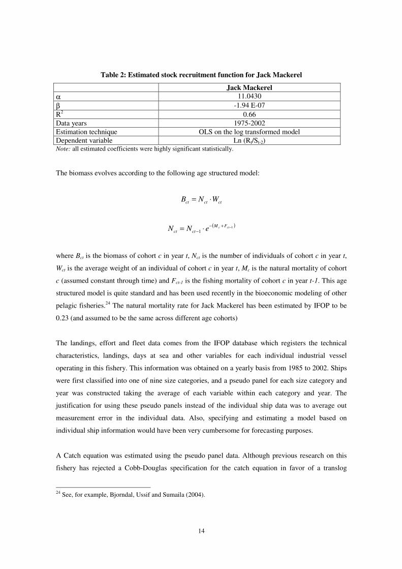
A Ricker stock recruitment function was specified and estimated for the Jack Mackerel.23 The

general form of the Ricker function is:

γβγα −⋅

− ⋅⋅= tStt eSR

where Rt is the number of recruits in year t, St-γ is the biomass (in tons) of spawning adults in the

population in the year t-γ, where γ is the age of recruits (γ =2 years in the case of Jack Mackerel).

The estimated parameters are presented in Table 2.

22 If it does not have sufficient quota left that year, next year’s quota is reduced. 23 The Ricker model is normally used for species with highly fluctuating recruitment, involving high fecundity as well as high natural mortality rates. Under favourable environmental conditions, species of this type can rapidly increase the range of their geographical distribution (for more details, see Yepes 2004, Begon and Mortimer 1986, and Haddon 2001).

14

Table 2: Estimated stock recruitment function for Jack Mackerel

Jack Mackerel α 11.0430 β -1.94 E-07 R2 0.66 Data years 1975-2002 Estimation technique OLS on the log transformed model Dependent variable Ln (Rt/St-2) Note: all estimated coefficients were highly significant statistically.

The biomass evolves according to the following age structured model:

ctctct WNB ⋅=

( )11

−+−− ⋅= ctc FM

ctct eNN

where Bct is the biomass of cohort c in year t, Nct is the number of individuals of cohort c in year t,

Wct is the average weight of an individual of cohort c in year t, Mc is the natural mortality of cohort

c (assumed constant through time) and Fct-1 is the fishing mortality of cohort c in year t-1. This age

structured model is quite standard and has been used recently in the bioeconomic modeling of other

pelagic fisheries.24 The natural mortality rate for Jack Mackerel has been estimated by IFOP to be

0.23 (and assumed to be the same across different age cohorts)

The landings, effort and fleet data comes from the IFOP database which registers the technical

characteristics, landings, days at sea and other variables for each individual industrial vessel

operating in this fishery. This information was obtained on a yearly basis from 1985 to 2002. Ships

were first classified into one of nine size categories, and a pseudo panel for each size category and

year was constructed taking the average of each variable within each category and year. The

justification for using these pseudo panels instead of the individual ship data was to average out

measurement error in the individual data. Also, specifying and estimating a model based on

individual ship information would have been very cumbersome for forecasting purposes.

A Catch equation was estimated using the pseudo panel data. Although previous research on this

fishery has rejected a Cobb-Douglas specification for the catch equation in favor of a translog

24 See, for example, Bjorndal, Ussif and Sumaila (2004).

15

specification (Peña-Torres, Basch and Vergara, 2003; Peña-Torres, Vergara and Basch, 2004), in

this paper we use the former functional form for simplicity. In addition, having quadratic terms in

the catch equation, as in a translog specification, may generate forecasting problems since variables

may become negative or grow to unrealistic levels much faster than in a linear model.

The estimated catch equation is presented in Table 3, where the dependent variable is the logarithm

of the annual catch (measured in tons) per vessel category. The equation was first estimated using

Generalized Least Squares to take into account the heteroskedasticity implicit in each observation of

the pseudo panel (since the number of individual ships in each size category and year was different).

In spite of this estimation strategy, the econometric tests rejected the null hypothesis of no

additional heteroskedasticity. Therefore, our preferred results were estimated using Feasible GLS.25

Table 3: Catch equation for Jack Mackerel

Variable Estimated Coefficients Constant -40.5258*** Dummy SC 230 to 370 m3 1.6299*** Dummy SC 370 to 510 m3 22.0791*** Dummy SC 510 to 650 m3 22.3925*** Dummy SC 650 to 790 m3 22.6695*** Dummy SC 790 to 930 m3 44.3212*** Dummy SC 930 to 1070 m3 44.4602*** Dummy SC 1070 to 1490 m3 44.6654*** Dummy SC above 1490 m3 44.8835*** Ln (days fishing) 0.5981** Ln (days fishing) x SC (370-790) 0.6160** Ln (days fishing) x SC (>790) 0.5606** Ln (biomass Jack Mackerel) 2.7175*** Ln (biomass J. Mackerel) x SC (370-790) -1.3845*** Ln (biomass J. Mackerel) x SC (>790) -2.6817*** Dummy 1997-2000 -0.6404*** Dummy 2001-2002 0.3999*** Number of observations 142 Estimation method Feasible GLS R2 ----

(if model estimated by GLS, R2 is 0.94) Note: *** indicates the parameter is significant at 1% level; ** indicates the parameter is significant at 5% level.

25 The null hypothesis of no autocorrelation could not be rejected. All these results are available from the authors upon request.

16

In general, the larger the ship (storage capacity below 230 m3 is the excluded category) the higher

is the constant of the catch equation. According to the parameter estimates, three broad categories of

vessels seem to emerge: those below 370 m3 of storage capacity, those above 370 m3 but below

790 and those above 790 m3. Within each category, the constant is very similar.

Annual fishing days (our measure of fishing effort) increase catches. The elasticity of catches to

fishing days is 0.60 for vessels below 370 m3 of storage capacity, but rises to 1,21 and 1,16 for

ships between 370 m3 and 790 m3, and ships above 790 m3, respectively. Thus, for larger ships the

catch equation exhibits nearly constant or slightly increasing returns to scale in fishing days. Similar

findings are reported in Peña-Torres et al. (2003 and 2004).

The biomass (calculated at the beginning of each year) is also statistically significant but its impact

on catches diminishes as ship size increases. This is consistent with the fact that, especially for

larger vessels, the use of electronic search equipments and the longer autonomy at sea, together with

the schooling behavior of pelagic fish species, could imply that biomass abundance may not

significantly affect catches but only until the biomass is close to collapsing (Clark, 1971 and 1985).

Finally, the effect of introducing the experimental fishing expeditions during the 1997-2000 period

served, ceteris paribus, to reduce annual catches of Jack Mackerel per vessel. This result is probably

dominated by the fact that in these expeditions ships had to undertake a number of days at sea in

search of schools, in a pre-allocated path, without being able to fish.26

Due to the estimation method used, no R2 is reported for the Jack Mackerel catch equation.27

However, as an indication of the fit of the model, the R2 of estimating this model by GLS was 0.94.

The estimated residuals were used to estimate the variance of the distribution of errors. Since the

presence of heteroskedasticity was detected, a different variance was estimated for each vessel size

category. These parameters, together with those estimated for the error distributions of the other

equations (including the stock recruitment equation), are used further below in the Monte Carlo

simulations.

26 Perhaps the dummy variable for this period should be interacted with days fishing if this explanation were true. However, for simplicity this variable was introduced in the constant of the equation. 27 An R2 measure is not reported by Stata for FGLS.

17

The next equation of the model is the Effort equation. That is, an equation that attempts to explain

the number of fishing days, per year, for each vessel size category. In order to specify the effort

equation, it is useful to develop a very simple model of effort determination.

In the southern industrial pelagic fishery, there are a few companies that own most of the fleet.28

Therefore, each company has to decide upon the optimal use of its own fleet. Lets assume initially

that each company hast one of each of two types of ships, that differ in terms of the marginal cost of

effort and its catch per effort relationship (catch equation). Lets assume to start with that an ITQ

system is in place. In this situation each company maximizes profits subject to the constraint that

total landings are equal to the assigned quota:

)()()()( 22112211 EcEcEhpEhpMax −−⋅+⋅=π

subject to

HEhEh =+ )()( 2211

In this model E1 and E2 are effort levels, c1 and c2 are the cost of effort functions, h1 and h2 are the

catch equations, where 1 and 2 denote the ship type. H is the individual quota of the company. The

first order condition for this maximization problem is:

( )i

i

i

i

Ec

Eh

p∂∂

=∂∂

⋅− λ

where � is a Lagrange multiplier associated with the restriction. Using the Cobb-Douglas catch

equation specified above and noting that the marginal cost of effort (days fishing) is constant we

arrive at the following equation for the determination of effort:

BpckEi

i

ii

iii ln

1ln

11

ln1

1ln

1

2

110 −

−−−

−−

+=α

αλαα (1)

In this equation, �1i and �2i are the coefficients of the catch equation related to the effort and

biomass stock, respectively. Therefore, under an ITQ system the determination of the logarithm of

28 Unfortunately, the IFOP database did not contain a variable identifying each ship’s ownership.

18

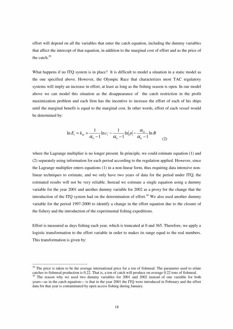
effort will depend on all the variables that enter the catch equation, including the dummy variables

that affect the intercept of that equation, in addition to the marginal cost of effort and as the price of

the catch.29

What happens if no ITQ system is in place? It is difficult to model a situation in a static model as

the one specified above. However, the Olympic Race that characterizes most TAC regulatory

systems will imply an increase in effort, at least as long as the fishing season is open. In our model

above we can model this situation as the disappearance of the catch restriction in the profit

maximization problem and each firm has the incentive to increase the effort of each of his ships

until the marginal benefit is equal to the marginal cost. In other words, effort of each vessel would

be determined by:

BpckEi

i

ii

iii ln

1ln

11

ln1

1ln

1

2

110 −

−−

−−

+=α

ααα (2)

where the Lagrange multiplier is no longer present. In principle, we could estimate equation (1) and

(2) separately using information for each period according to the regulation applied. However, since

the Lagrange multiplier enters equations (1) in a non-linear form, thus requiring data intensive non-

linear techniques to estimate, and we only have two years of data for the period under ITQ, the

estimated results will not be very reliable. Instead we estimate a single equation using a dummy

variable for the year 2001 and another dummy variable for 2002 as a proxy for the change that the

introduction of the ITQ system had on the determination of effort.30 We also used another dummy

variable for the period 1997-2000 to identify a change in the effort equation due to the closure of

the fishery and the introduction of the experimental fishing expeditions.

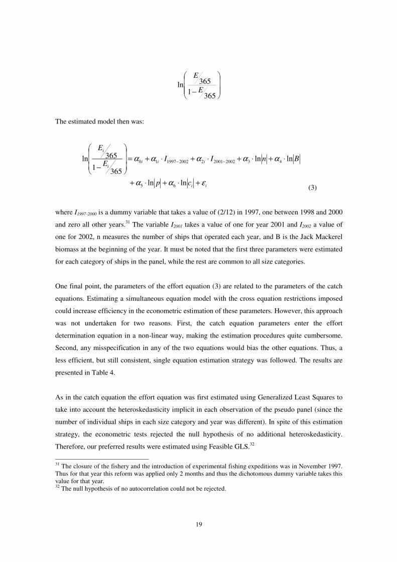
Effort is measured as days fishing each year, which is truncated at 0 and 365. Therefore, we apply a

logistic transformation to the effort variable in order to makes its range equal to the real numbers.

This transformation is given by:

29 The price is taken to be the average international price for a ton of fishmeal. The parameter used to relate catches to fishmeal production is 0.22. That is, a ton of catch will produce on average 0.22 tons of fishmeal. 30 The reason why we used two dummy variables for 2001 and 2002 instead of one variable for both yearsas in the catch equation is that in the year 2001 the ITQ were introduced in February and the effort data for that year is contaminated by open access fishing during January.

19

���

�

�

���

�

�

− 3651365lnE

E

The estimated model then was:

ii

iiii

i

cp

BnIIE

E

εαα

ααααα

+⋅+⋅+

⋅+⋅+⋅+⋅+=���

�

�

���

�

�

−−−

lnln

lnln

3651365ln

65

432002200122002199710

(3)

where I1997-2000 is a dummy variable that takes a value of (2/12) in 1997, one between 1998 and 2000

and zero all other years.31 The variable I2001 takes a value of one for year 2001 and I2002 a value of

one for 2002, n measures the number of ships that operated each year, and B is the Jack Mackerel

biomass at the beginning of the year. It must be noted that the first three parameters were estimated

for each category of ships in the panel, while the rest are common to all size categories.

One final point, the parameters of the effort equation (3) are related to the parameters of the catch

equations. Estimating a simultaneous equation model with the cross equation restrictions imposed

could increase efficiency in the econometric estimation of these parameters. However, this approach

was not undertaken for two reasons. First, the catch equation parameters enter the effort

determination equation in a non-linear way, making the estimation procedures quite cumbersome.

Second, any misspecification in any of the two equations would bias the other equations. Thus, a

less efficient, but still consistent, single equation estimation strategy was followed. The results are

presented in Table 4.

As in the catch equation the effort equation was first estimated using Generalized Least Squares to

take into account the heteroskedasticity implicit in each observation of the pseudo panel (since the

number of individual ships in each size category and year was different). In spite of this estimation

strategy, the econometric tests rejected the null hypothesis of no additional heteroskedasticity.

Therefore, our preferred results were estimated using Feasible GLS.32

31 The closure of the fishery and the introduction of experimental fishing expeditions was in November 1997. Thus for that year this reform was applied only 2 months and thus the dichotomous dummy variable takes this value for that year. 32 The null hypothesis of no autocorrelation could not be rejected.

20

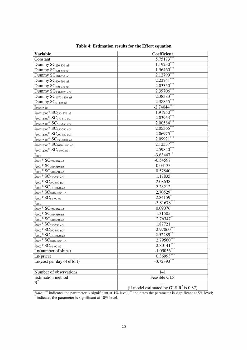
Table 4: Estimation results for the Effort equation

Variable Coefficient Constant 5.75173*** Dummy SC230-370 m3 1.19230*** Dummy SC370-510 m3 1.56460*** Dummy SC510-650 m3 2.12799*** Dummy SC650-790 m3 2.22741*** Dummy SC790-930 m3 2.03350*** Dummy SC930-1070 m3 2.39706*** Dummy SC1070-1490 m3 2.38383*** Dummy SC>1490 m3 2.38855*** I1997-2000 -2.74044*** I1997-2000* SC230- 370 m3 1.91950*** I1997-2000* SC370-510 m3 2.03953*** I1997-2000* SC510-650 m3 2.00584*** I1997-2000* SC650-790 m3 2.05365*** I1997-2000* SC790-930 m3 2.06975*** I1997-2000* SC930-1070 m3 2.09921*** I1997-2000* SC1070-1490 m3 2.12537*** I1997-2000* SC>1490 m3 2.59840*** I2001 -3.63447** I2001* SC230-370 m3 -0.54597 I2001* SC370-510 m3 -0.03133 I2001* SC510-650 m3 0.57840 I2001* SC650-790 m3 1.17835 I2001* SC790-930 m3 2.08638 I2001* SC930-1070 m3 2.28212 I2001* SC1070-1490 m3 2.70529* I2001* SC>1490 m3 2.84159* I2002 -3.81678*** I2002* SC230-370 m3 0.09076 I2002* SC370-510 m3 1.31505 I2002* SC510-650 m3 2.76347** I2002* SC650-790 m3 1.87721 I2002* SC790-930 m3 2.97860*** I2002* SC930-1070 m3 2.52289** I2002* SC1070-1490 m3 2.79560*** I2002* SC>1490 m3 2.80141*** Ln(number of ships) -1.05056*** Ln(price) 0.36993*** Ln(cost per day of effort) -0.72393*** Number of observations 141 Estimation method Feasible GLS R2 ---

(if model estimated by GLS R2 is 0.87) Note: *** indicates the parameter is significant at 1% level; ** indicates the parameter is significant at 5% level; * indicates the parameter is significant at 10% level.

21

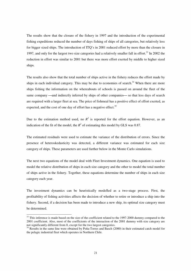
The results show that the closure of the fishery in 1997 and the introduction of the experimental

fishing expeditions reduced the number of days fishing of ships of all categories, but relatively less

for bigger sized ships. The introduction of ITQ’s in 2001 reduced effort by more than the closure in

1997, and only for the largest two size categories had a relatively smaller fall in effort.33 In 2002 the

reduction in effort was similar to 2001 but there was more effort exerted by middle to higher sized

ships.

The results also show that the total number of ships active in the fishery reduces the effort made by

ships in each individual category. This may be due to economies of search.34 When there are more

ships fishing the information on the whereabouts of schools is passed on around the fleet of the

same company and indirectly inferred by ships of other companies so that less days of search

are required with a larger fleet at sea. The price of fishmeal has a positive effect of effort exerted, as

expected, and the cost of one day of effort has a negative effect.35

Due to the estimation method used, no R2 is reported for the effort equation. However, as an

indication of the fit of the model, the R2 of estimating this model by GLS was 0.87.

The estimated residuals were used to estimate the variance of the distribution of errors. Since the

presence of heteroskedasticity was detected, a different variance was estimated for each size

category of ships. These parameters are used further below in the Monte Carlo simulations.

The next two equations of the model deal with Fleet Investment dynamics. One equation is used to

model the relative distribution of ships in each size category and the other to model the total number

of ships active in the fishery. Together, these equations determine the number of ships in each size

category each year.

The investment dynamics can be heuristically modelled as a two-stage process. First, the

profitability of fishing activities affects the decision of whether to retire or introduce a ship into the

fishery. Second, if a decision has been made to introduce a new ship, its optimal size category must

be determined.

33 This inference is made based on the size of the coefficient related to the 1997-2000 dummy compared to the 2001 coefficient. Also, most of the coefficients of the interaction of the 2001 dummy with size category are not significantly different from 0, except for the two largest categories. 34 Results in the same line were obtained by Peña-Torres and Basch (2000) in their estimated catch model for the pelagic industrial fleet which operates in Northern Chile.

22

The economic returns to fishing are inherently uncertain, especially in this pelagic fishery geared

towards the production of fishmeal. Being a traded commodity its price is determined on the world

market and can be quite volatile depending on global economic activity. On the other hand, the

environmental uncertainties related to fish stock abundance, migration and other effects makes

catching fish an uncertain activity in itself. Additionally, fleet investment usually implies a high

degree of value specificity and therefore ex-post sunk costs.

Modern investment theory predicts that the decision to undertake or abandon a value-specific

investment project under uncertainty will depend on certain variables reaching a threshold level.36

In particular, if we define E(V/t) as the expected net present value of an investment project

estimated using all the information available until t, then theory predicts that the project will be

undertaken when:

( ) 0/ >> αtVE

for some positive parameter �. Notice that under uncertainty an investor in a value-specific project

will decide to undertake an investment when the net present value of this investment is strictly

above zero by a certain amount. The reason for this is that there is an option value of postponing an

investment decision until more information is available. Thus only when the net present value of

undertaking the project now is above this option value will the decision be made to go ahead with

the project. The analogous condition for abandoning a project is:

( ) 0/ << βtVE .

Under uncertainty an investor will not abandon a project when the net present value reaches zero,

only when this value is sufficiently below zero. When the expected value of the project is between �

and �, the optimal decision is not to invest, if the project has not yet begun, and to continue

operating, if the project is already in operation.

The particular values of � and � will depend on various factors, including the properties of the

stochastic process followed by the underlying random variables that affect the value of the project

(in particular the variance of the distributions), the amount of the required initial investment and

35 The cost of effort only includes the variable fuel, labor and material costs of fishing trips.

23

possible exit costs. These last costs include payments required if operation ceases (severance

payments for example) as well as any sunk cost of the project.

As shown by Dixit and Pindyck (1994), the higher is the amount of the initial investment, the higher

the values of � and �. Thus, from the point of view of the current model, these parameters should be

allowed to differ for different ship size categories.

Assume that investors observe the results of each ship in year t. They can then form an idea of the

relative profitability of each type of vessel. Assume for the moment that firms can renew their fleet

each year without any adjustment cost. Then, each firm will decide to have a fleet composed of

ships type i, where:

0)/()/( >−=− jjjii tVEMaxtVE αα

where j indexes all types of ships. In other words, they will choose the most profitable size category

among those available. The econometrician does not directly observe E(Vj/t) – �j but he does

observe a proxy for this value in the form of the current profitability of each type of ship:

( ) jtjjt tVE επ += /

where �jt is the profitability of ship type j in year t and �jt is an error assumed to be independently

distributed among size categories and year. Besides measurement error, this error term can also be

attributed to the possible dispersion of information as regards the relative profitability of each type

of ship among firms.37 Therefore, the probability that ship type i is the preferred type in year t is

given by:

[ ][ ]jtjjtjitiit Max εαπεαπ −+=−+Pr.

36 For a modern exposition of the theory see Dixit and Pindyck (1994). 37 In order for current profitability to proxy for the value of the project, the underlying stochastic variables must have the Markov property. That is, the expected value of each variable for the next period must be a function of the value of that variable in the current period only, not past values of these variables. In general, the stochastic processes of commodity prices (such as fishmeal) have this property.

24

If it is further assumed that the �jt have an extreme value distribution, then the probability of that

ship type i is the preferred type in year t has a multinomial logistic distribution:

[ ][ ]�

=

+

+

=−+=−+ 9

1

Pr

j

jtjjtjitiitjjt

iit

e

eMax

απ

απ

εαπεαπ

The above expression gives the ideal relative frequency of ship type i in year t assuming there are

no adjustment costs:

�=

+

+

= 9

1

*

j

itjjt

iit

e

ef

απ

απ

If we define a base category (ship type b, for example), then a simple transformation of the above

equation leads to:

( ) ( )bibtitbtit ff ααππ −+−=− ** lnln.

This last condition states that the logarithm of the relative ideal frequency of ships type i and b will

depend on the relative profitability of each type of ship and the relative value of the threshold

investment parameters.

Until now it was assumed that there were no adjustment costs. This is clearly unrealistic. A better

specification would posit that firms face adjustment costs and thus adjust their capital stock only

partially each period in the direction of their optimal composition. Thus, the fleet composition in the

current period is equal to last period’s composition plus an adjustment due to the difference

between last period’s optimal and real relative fleet composition:

[ ] [ ] [ ]( )11*

1*

111 lnlnlnlnlnlnlnln −−−−−− −−−⋅+−=− btitbtitbtitbtit ffffffff λ

25

where the parameter � measures the speed of adjustment. This parameter must be between 0 (very

slow adjustment) and 1 (very fast adjustment). Substituting for the condition of optimal relative

fleet composition gives the following model:

( ) ( )( ) ( ) [ ]1111 lnln1lnln −−−− −⋅−+−+−⋅=− btitbibtitbtit ffff λααππλ.

Thus, the model estimated was:

( ) [ ] itbtitbtitibtit ffff εβππββ +−⋅+−⋅+=− −−−− 1121110 lnlnlnln.

Since each variable is defined relative to the base category, which we defined as the category of

ships between 510 and 650 m3 of storage capacity, the observations for the base category are not

used in the estimation.

The profitability of each type of ship was empirically defined as:

( )i

FCitit

Eitit

fmfmt

it I

cEcLcpt

−⋅−⋅⋅−=

θπ

where ptfm is the price of fishmeal in year t, ct

fm is the cost of processing fishmeal in year t, Lit is total

landings (including species other than Jack Mackerel) by the average ship of category i in year t, �

is a technical parameter to convert tons of fish into fishmeal, citE is the cost per unit of effort, Eit is

the effort level (days fishing per year) by the average ship of category i in year t, citFC is the fixed

cost related to ships of type i in year t (including routine maintenance costs) and Ii is the investment

cost of a ship type i.

All the cost information was constructed from company data and expert opinions for the period

1985 to 2002. The investment cost for each type of vessel was estimated based on published

information in trade journals as well as expert opinion. Due to insufficient information this cost

does not vary by year. The fishmeal price is the yearly average price of fishmeal exports according

to the international trade statistics of the Central Bank of Chile. The � parameter was set to the

average over the 1985 to 2002 period, which was 0.22.

26

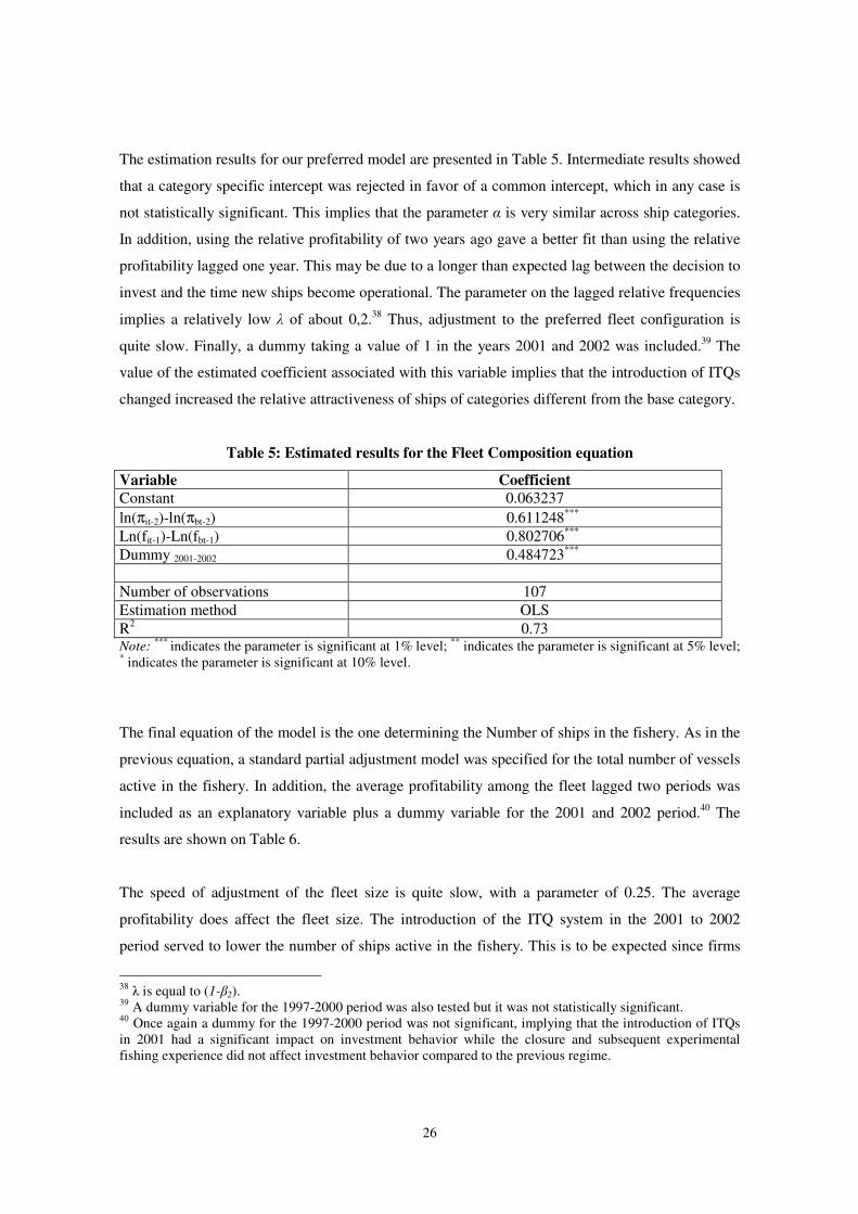
The estimation results for our preferred model are presented in Table 5. Intermediate results showed

that a category specific intercept was rejected in favor of a common intercept, which in any case is

not statistically significant. This implies that the parameter � is very similar across ship categories.

In addition, using the relative profitability of two years ago gave a better fit than using the relative

profitability lagged one year. This may be due to a longer than expected lag between the decision to

invest and the time new ships become operational. The parameter on the lagged relative frequencies

implies a relatively low � of about 0,2.38 Thus, adjustment to the preferred fleet configuration is

quite slow. Finally, a dummy taking a value of 1 in the years 2001 and 2002 was included.39 The

value of the estimated coefficient associated with this variable implies that the introduction of ITQs

changed increased the relative attractiveness of ships of categories different from the base category.

Table 5: Estimated results for the Fleet Composition equation

Variable Coefficient Constant 0.063237 ln(πit-2)-ln(πbt-2) 0.611248*** Ln(fit-1)-Ln(fbt-1) 0.802706*** Dummy 2001-2002 0.484723*** Number of observations 107 Estimation method OLS R2 0.73 Note: *** indicates the parameter is significant at 1% level; ** indicates the parameter is significant at 5% level; * indicates the parameter is significant at 10% level.

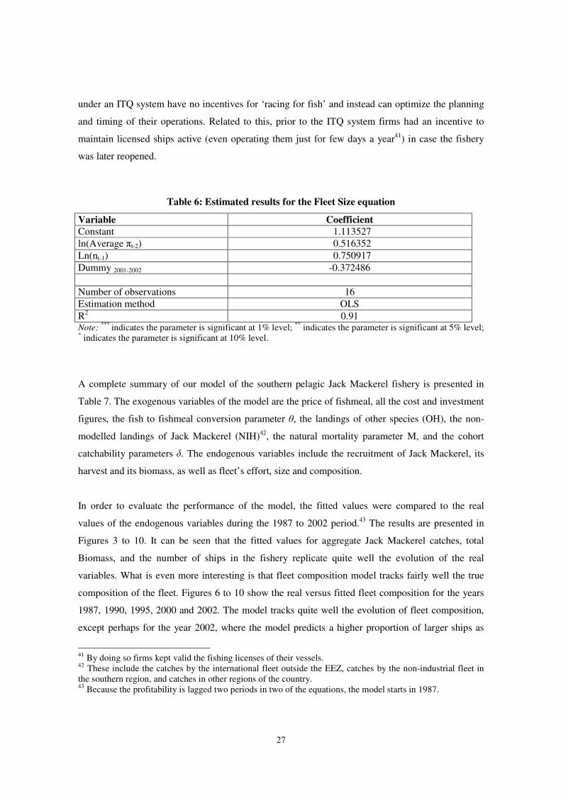
The final equation of the model is the one determining the Number of ships in the fishery. As in the

previous equation, a standard partial adjustment model was specified for the total number of vessels

active in the fishery. In addition, the average profitability among the fleet lagged two periods was

included as an explanatory variable plus a dummy variable for the 2001 and 2002 period.40 The

results are shown on Table 6.

The speed of adjustment of the fleet size is quite slow, with a parameter of 0.25. The average

profitability does affect the fleet size. The introduction of the ITQ system in the 2001 to 2002

period served to lower the number of ships active in the fishery. This is to be expected since firms

38 � is equal to (1-�2). 39 A dummy variable for the 1997-2000 period was also tested but it was not statistically significant. 40 Once again a dummy for the 1997-2000 period was not significant, implying that the introduction of ITQs in 2001 had a significant impact on investment behavior while the closure and subsequent experimental fishing experience did not affect investment behavior compared to the previous regime.

27

under an ITQ system have no incentives for ‘racing for fish’ and instead can optimize the planning

and timing of their operations. Related to this, prior to the ITQ system firms had an incentive to

maintain licensed ships active (even operating them just for few days a year41) in case the fishery

was later reopened.

Table 6: Estimated results for the Fleet Size equation

Variable Coefficient Constant 1.113527 ln(Average �t-2) 0.516352 Ln(nt-1) 0.750917 Dummy 2001-2002 -0.372486 Number of observations 16 Estimation method OLS R2 0.91 Note: *** indicates the parameter is significant at 1% level; ** indicates the parameter is significant at 5% level; * indicates the parameter is significant at 10% level.

A complete summary of our model of the southern pelagic Jack Mackerel fishery is presented in

Table 7. The exogenous variables of the model are the price of fishmeal, all the cost and investment

figures, the fish to fishmeal conversion parameter �, the landings of other species (OH), the non-

modelled landings of Jack Mackerel (NIH)42, the natural mortality parameter M, and the cohort

catchability parameters �. The endogenous variables include the recruitment of Jack Mackerel, its

harvest and its biomass, as well as fleet’s effort, size and composition.

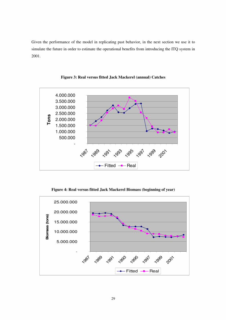
In order to evaluate the performance of the model, the fitted values were compared to the real

values of the endogenous variables during the 1987 to 2002 period.43 The results are presented in

Figures 3 to 10. It can be seen that the fitted values for aggregate Jack Mackerel catches, total

Biomass, and the number of ships in the fishery replicate quite well the evolution of the real

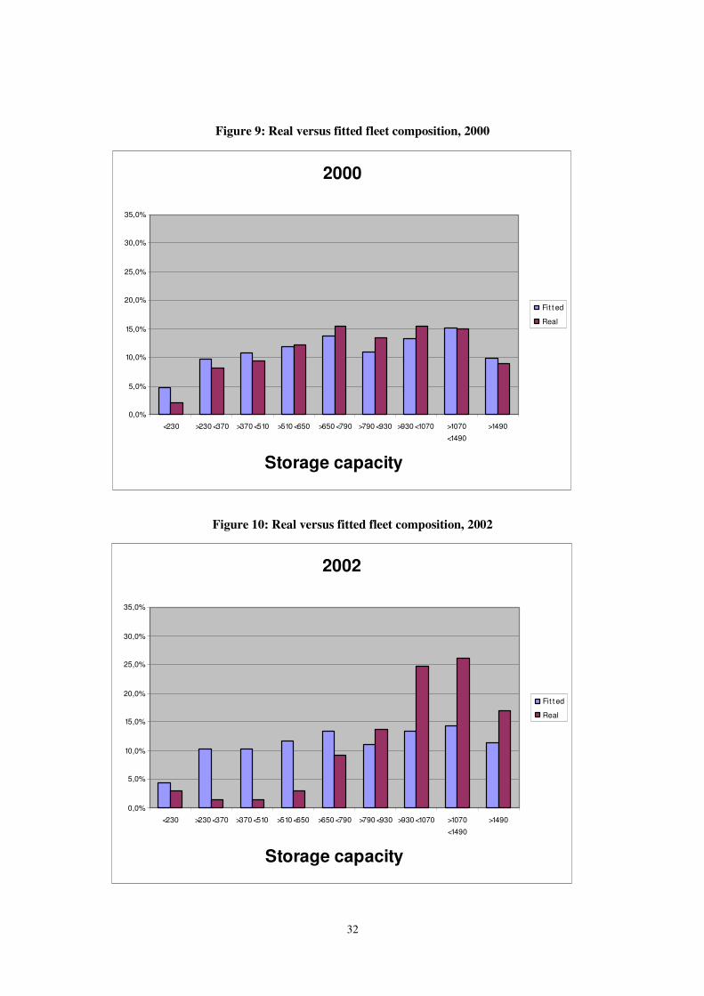
variables. What is even more interesting is that fleet composition model tracks fairly well the true

composition of the fleet. Figures 6 to 10 show the real versus fitted fleet composition for the years

1987, 1990, 1995, 2000 and 2002. The model tracks quite well the evolution of fleet composition,

except perhaps for the year 2002, where the model predicts a higher proportion of larger ships as

41 By doing so firms kept valid the fishing licenses of their vessels. 42 These include the catches by the international fleet outside the EEZ, catches by the non-industrial fleet in the southern region, and catches in other regions of the country. 43 Because the profitability is lagged two periods in two of the equations, the model starts in 1987.

28

compared to what happened in reality. However, for such complex phenomena the model is quite

satisfactory.

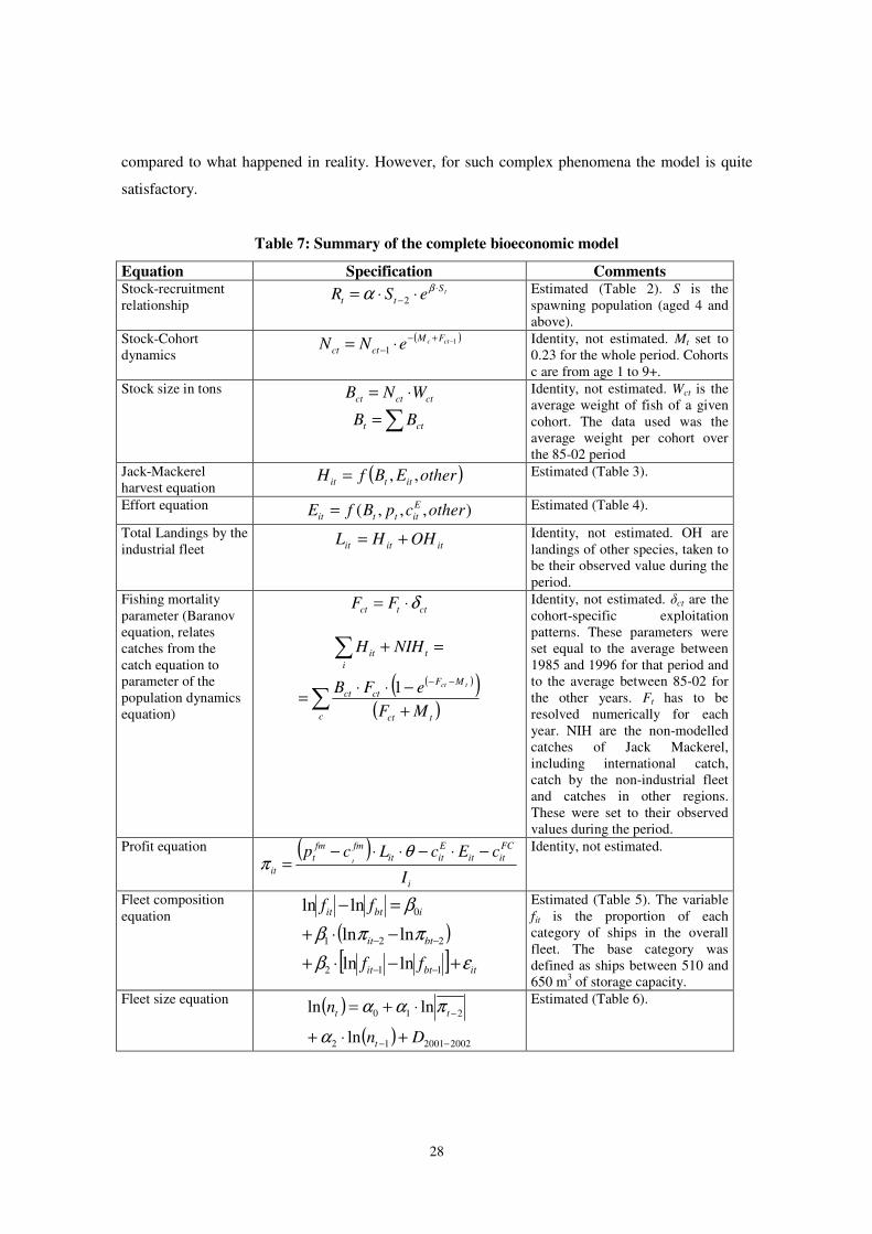
Table 7: Summary of the complete bioeconomic model

Equation Specification Comments Stock-recruitment relationship

tStt eSR ⋅− ⋅⋅= βα 2

Estimated (Table 2). S is the spawning population (aged 4 and above).

Stock-Cohort dynamics

( )11

−+−− ⋅= ctc FM

ctct eNN

Identity, not estimated. Mt set to 0.23 for the whole period. Cohorts c are from age 1 to 9+.

Stock size in tons ctctct WNB ⋅=

�= ctt BB

Identity, not estimated. Wct is the average weight of fish of a given cohort. The data used was the average weight per cohort over the 85-02 period

Jack-Mackerel harvest equation

( )otherEBfH ittit ,,= Estimated (Table 3).

Effort equation ),,,( othercpBfE Eitttit =

Estimated (Table 4).

Total Landings by the industrial fleet ititit OHHL +=

Identity, not estimated. OH are landings of other species, taken to be their observed value during the period.

Fishing mortality parameter (Baranov equation, relates catches from the catch equation to parameter of the population dynamics equation)

cttct FF δ⋅=

( )( )( )�

�

+−⋅⋅=

=+

−−

c tct

MFctct

ti

it

MFeFB

NIHH

tct1

Identity, not estimated. �ct are the cohort-specific exploitation patterns. These parameters were set equal to the average between 1985 and 1996 for that period and to the average between 85-02 for the other years. Ft has to be resolved numerically for each year. NIH are the non-modelled catches of Jack Mackerel, including international catch, catch by the non-industrial fleet and catches in other regions. These were set to their observed values during the period.

Profit equation ( )i

FCitit

Eitit

fmfmt

it I

cEcLcpt

−⋅−⋅⋅−=

θπ

Identity, not estimated.

Fleet composition equation

( )[ ] itbtit

btit

ibtit

ff

ff

εβππβ

β

+−⋅+−⋅+=−

−−

−−

112

221

0

lnln

lnln

lnln

Estimated (Table 5). The variable fit is the proportion of each category of ships in the overall fleet. The base category was defined as ships between 510 and 650 m3 of storage capacity.

Fleet size equation ( )( ) 2002200112

210

ln

lnln

−−

−

+⋅+

⋅+=

Dn

n

t

tt

α

παα

Estimated (Table 6).

29

Given the performance of the model in replicating past behavior, in the next section we use it to

simulate the future in order to estimate the operational benefits from introducing the ITQ system in

2001.

Figure 3: Real versus fitted Jack Mackerel (annual) Catches

Figure 4: Real versus fitted Jack Mackerel Biomass (beginning of year)

-

5.000.000

10.000.000

15.000.000

20.000.000

25.000.000

1987

1989

1991

1993

1995

1997

1999

2001

Bio

mas

s (t

ons)

Fitted Real

- 500.000

1.000.000 1.500.000 2.000.000 2.500.000 3.000.000 3.500.000 4.000.000

1987

1989

1991

1993

1995

1997

1999

2001

Ton

s

Fitted Real

30

Figure 5: Real versus fitted Fleet Size

(Total Number of Operating Industrial Vessels)

Figure 6: Real versus fitted Fleet Composition, 1987

- 20 40 60 80

100 120 140 160 180 200

1987

1989

1991

1993

1995

1997

1999

2001

Num

ber

Fitted Real

1987

0,0%

5,0%

10,0%

15,0%

20,0%

25,0%

30,0%

35,0%

<230 >230 <370 >370 <510 >510 <650 >650 <790 >790 <930 >930 <1070 >1070 <1490 >1490

Storage capacity

Fi tted

Real

31

Figure 7: Real versus fitted fleet composition, 1990

Figure 8: Real versus fitted fleet composition, 1995

1990

0,0%

5,0%

10,0%

15,0%

20,0%

25,0%

30,0%

35,0%

<230 >230 <370 >370 <510 >510 <650 >650 <790 >790 <930 >930 <1070 >1070

<1490

>1490

Storage capacity

Fit t ed

Real

1995

0,0%

5,0%

10,0%

15,0%

20,0%

25,0%

30,0%

35,0%

<230 >230 <370 >370 <510 >510 <650 >650 <790 >790 <930 >930 <1070 >1070

<1490

>1490

Storage capacity

Fit t ed

Real

32

Figure 9: Real versus fitted fleet composition, 2000

Figure 10: Real versus fitted fleet composition, 2002

2000

0,0%

5,0%

10,0%

15,0%

20,0%

25,0%

30,0%

35,0%

<230 >230 <370 >370 <510 >510 <650 >650 <790 >790 <930 >930 <1070 >1070

<1490

>1490

Storage capacity

Fit t ed

Real

2002

0,0%

5,0%

10,0%

15,0%

20,0%

25,0%

30,0%

35,0%

<230 >230 <370 >370 <510 >510 <650 >650 <790 >790 <930 >930 <1070 >1070

<1490

>1490

Storage capacity

Fit t ed

Real

33

5. Monte Carlo simulations

The model was used to generate 100 simulations for the period 2001 to 2020.44 For each simulation,

draws were taken from the error distributions of the estimated equations. There were 20 such

distributions, 9 (one for each ship category) for the catch equation, 9 (one for each ship category)

for the effort equation, 1 for the fleet composition equation and 1 for the fleet size equation. All

distributions were assumed to be log-normally distributed with a standard error equal to the

estimated value from the econometric results and mean zero of the logarithm of the variable.

Although formal tests usually reject the null hypothesis of log-normality, a graphical inspection of

the residuals of each equation reveals that it is a good approximation. The alternative would have

been to have taken samples from the empirical distribution of residuals for each equation. However,

since the sample period is quite short (1985 to 2002), for most cases this distribution has few data

points and would probably have made the results more erratic.

In order to make simulations certain assumptions have to be made with respect to the exogenous

variables of the model. With respect to the price of fishmeal, it was set to US$581 each year, which

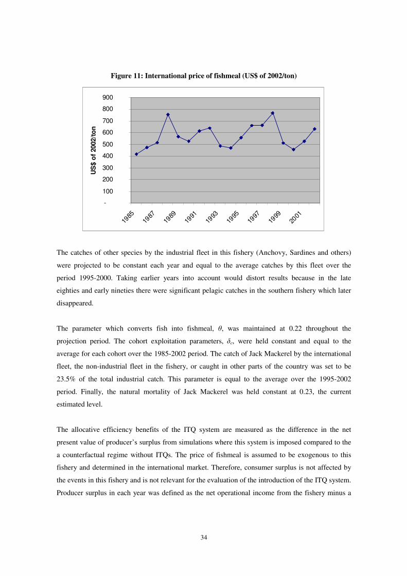
corresponds to the average real price between 1985 and 2002. Figure 11 shows the real price of

fishmeal (constant 2002 prices) during the whole sample period. Notice that in the year 2001 and

2002 we did not use the true observed price but rather the average over 1985 to 2002. The reason is

that to evaluate the introduction of the ITQ system simulations had to start in 2001. Thus, our

results are from the viewpoint of evaluating the introduction of this system in the year 2000.

It can be seen that this price has a cyclical behavior. Although future research should attempt to

model this price in order to project into the future, in this study it was held constant at the sample

period average. One possible justification for this approach is that the data on costs was held

constant at the 2002 level in all simulations. There was scant information to model the evolution of

future costs (including fuel prices and investment costs), so the only reasonable assumption was to

maintain their last observed level. Maintaining prices constant is consistent with this treatment for

cost variables.

44 Although more simulations would have been ideal, in one scenario presented below (with TAC) the model takes 51 seconds to resolve one simulation. This is due to the fact that numerical techniques have to be used to find the effort and F parameter in each of the 18 years of the simulation. Therefore, more than 100 simulations would be quite costly in terms of research time.

34

Figure 11: International price of fishmeal (US$ of 2002/ton)

The catches of other species by the industrial fleet in this fishery (Anchovy, Sardines and others)

were projected to be constant each year and equal to the average catches by this fleet over the

period 1995-2000. Taking earlier years into account would distort results because in the late

eighties and early nineties there were significant pelagic catches in the southern fishery which later

disappeared.

The parameter which converts fish into fishmeal, �, was maintained at 0.22 throughout the

projection period. The cohort exploitation parameters, �c, were held constant and equal to the

average for each cohort over the 1985-2002 period. The catch of Jack Mackerel by the international

fleet, the non-industrial fleet in the fishery, or caught in other parts of the country was set to be

23.5% of the total industrial catch. This parameter is equal to the average over the 1995-2002

period. Finally, the natural mortality of Jack Mackerel was held constant at 0.23, the current

estimated level.

The allocative efficiency benefits of the ITQ system are measured as the difference in the net

present value of producer’s surplus from simulations where this system is imposed compared to the

a counterfactual regime without ITQs. The price of fishmeal is assumed to be exogenous to this

fishery and determined in the international market. Therefore, consumer surplus is not affected by

the events in this fishery and is not relevant for the evaluation of the introduction of the ITQ system.

Producer surplus in each year was defined as the net operational income from the fishery minus a

-

100

200

300

400

500

600

700

800

900

1985

1987

1989

1991

1993

1995

1997

1999

2001

US

$ of

200

2/to

n

35

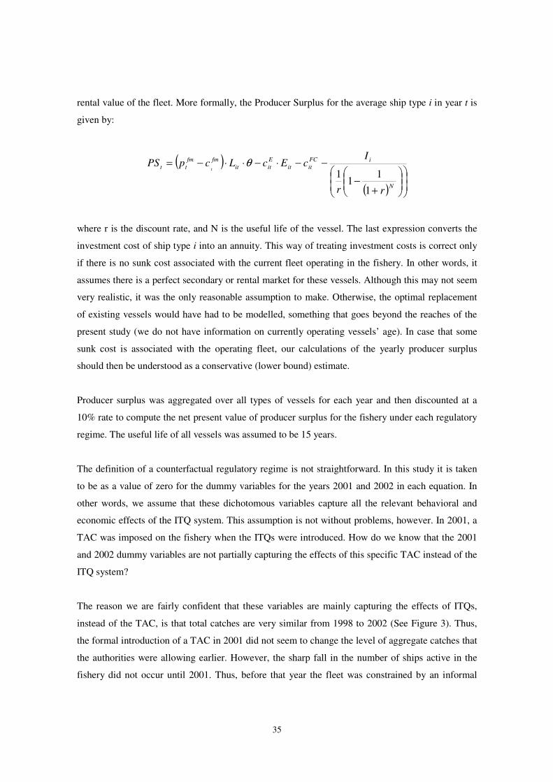
rental value of the fleet. More formally, the Producer Surplus for the average ship type i in year t is

given by:

( )( ) �

�

�

�

��

�

����

����

�

+−

−−⋅−⋅⋅−=

N

iFCitit

Eitit

fmfmtt

rr

IcEcLcpPS

t

1

11

1θ

where r is the discount rate, and N is the useful life of the vessel. The last expression converts the

investment cost of ship type i into an annuity. This way of treating investment costs is correct only

if there is no sunk cost associated with the current fleet operating in the fishery. In other words, it

assumes there is a perfect secondary or rental market for these vessels. Although this may not seem

very realistic, it was the only reasonable assumption to make. Otherwise, the optimal replacement

of existing vessels would have had to be modelled, something that goes beyond the reaches of the

present study (we do not have information on currently operating vessels’ age). In case that some

sunk cost is associated with the operating fleet, our calculations of the yearly producer surplus

should then be understood as a conservative (lower bound) estimate.

Producer surplus was aggregated over all types of vessels for each year and then discounted at a

10% rate to compute the net present value of producer surplus for the fishery under each regulatory

regime. The useful life of all vessels was assumed to be 15 years.

The definition of a counterfactual regulatory regime is not straightforward. In this study it is taken

to be as a value of zero for the dummy variables for the years 2001 and 2002 in each equation. In

other words, we assume that these dichotomous variables capture all the relevant behavioral and

economic effects of the ITQ system. This assumption is not without problems, however. In 2001, a

TAC was imposed on the fishery when the ITQs were introduced. How do we know that the 2001

and 2002 dummy variables are not partially capturing the effects of this specific TAC instead of the

ITQ system?

The reason we are fairly confident that these variables are mainly capturing the effects of ITQs,

instead of the TAC, is that total catches are very similar from 1998 to 2002 (See Figure 3). Thus,

the formal introduction of a TAC in 2001 did not seem to change the level of aggregate catches that

the authorities were allowing earlier. However, the sharp fall in the number of ships active in the

fishery did not occur until 2001. Thus, before that year the fleet was constrained by an informal

36

TAC (through the control of the fishing expeditions) of a similar level as after 2001, but it was not

until 2001 with the introduction of ITQs that firms optimized their fleet and operations.

Another complication is raised by the presence of TACs in the fishery after 2001. What should be

the level of TACs from 2003 to 2020? In this paper as our base scenario we assume that from 2003

to 2020, a TAC similar to current levels is imposed for each year. The official TAC for Jack

Mackerel was 1,450,000 tons and 1,488,500 tons in 2003 and 2004 respectively. These limits

include all catches of the resource, not just from the Southern pelagic industrial fleet. For this fleet,

the relevant TAC was close to 1,100,000 tons each year and this was the value used for all years.45

One final comment before presenting the results: It is possible that the stock collapses to zero in

some scenario. In this case, Jack Mackerel catches are zero from then on, but the fleet remains

active catching other resources. The fall in profitability that this implies will gradually reduce the

size of the fleet.

5.1 Results

Table 9 presents the results for a TAC of 1.1 million tons for each year. Since the TAC is the same

for each simulation, the catch and stock dynamics are identical with and without the ITQ system.

Thus, their corresponding averages over the 100 simulations are also the same. From the results it

can be seen that the biomass increases at the beginning of the projection period and later falls.

The main difference between both scenarios is that under an ITQ system the number of ships in the

fishery remains relatively constant, even decreasing slightly. On the other hand, without the ITQ

system the number of ships increases dramatically.46 This in turn implies that the net producer

surplus from the fishery is about US$366 million higher under an ITQ system than without it.

45 In each simulation the model was resolved by finding the level of effort that made aggregate catches equal to the TAC. This had to be done numerically. 46 In practice, the initial unemployment triggered by the reduction in the number of operating ships (under the real ITQ system) has later been partially counteracted by increases in the number of regular jobs in the fish processing sector, the latter being the result of ITQ-triggered changes in the final productive mix towards higher value added processing activities (which are also more labor intensive than fishing effort activities). Unfortunately, we had no access to more detailed information about ITQ-triggered effects upon labor markets and final processing production.

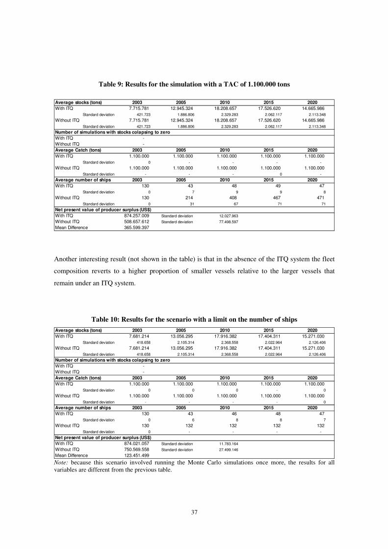
37

Table 9: Results for the simulation with a TAC of 1.100.000 tons

Another interesting result (not shown in the table) is that in the absence of the ITQ system the fleet

composition reverts to a higher proportion of smaller vessels relative to the larger vessels that

remain under an ITQ system.

Table 10: Results for the scenario with a limit on the number of ships

Note: because this scenario involved running the Monte Carlo simulations once more, the results for all variables are different from the previous table.

Average stocks (tons) 2003 2005 2010 2015 2020With ITQ 7.715.781 12.945.324 18.208.657 17.526.620 14.665.986

Standard deviation 421.723 1.886.806 2.329.283 2.062.117 2.113.348 Without ITQ 7.715.781 12.945.324 18.208.657 17.526.620 14.665.986

Standard deviation 421.723 1.886.806 2.329.283 2.062.117 2.113.348 Number of simulations with stocks colapsing to zeroWith ITQ - Without ITQ - Average Catch (tons) 2003 2005 2010 2015 2020With ITQ 1.100.000 1.100.000 1.100.000 1.100.000 1.100.000

Standard deviation 0 - - - - Without ITQ 1.100.000 1.100.000 1.100.000 1.100.000 1.100.000

Standard deviation - - - 0 - Average number of ships 2003 2005 2010 2015 2020With ITQ 130 43 48 49 47

Standard deviation 0 7 9 9 8 Without ITQ 130 214 408 467 471

Standard deviation 0 31 67 71 71 Net present value of producer surplus (US$)With ITQ 874.257.009 Standard deviation 12.027.963 Without ITQ 508.657.612 Standard deviation 77.498.597 Mean Difference 365.599.397

Average stocks (tons) 2003 2005 2010 2015 2020With ITQ 7.681.214 13.056.295 17.916.382 17.404.311 15.271.030

Standard deviation 418.658 2.105.314 2.368.558 2.022.964 2.126.406 Without ITQ 7.681.214 13.056.295 17.916.382 17.404.311 15.271.030

Standard deviation 418.658 2.105.314 2.368.558 2.022.964 2.126.406 Number of simulations with stocks colapsing to zeroWith ITQ - Without ITQ - Average Catch (tons) 2003 2005 2010 2015 2020With ITQ 1.100.000 1.100.000 1.100.000 1.100.000 1.100.000

Standard deviation 0 0 0 - 0 Without ITQ 1.100.000 1.100.000 1.100.000 1.100.000 1.100.000

Standard deviation - - - - 0 Average number of ships 2003 2005 2010 2015 2020With ITQ 130 43 46 48 47

Standard deviation 0 6 8 8 7 Without ITQ 130 132 132 132 132

Standard deviation 0 - - - - Net present value of producer surplus (US$)With ITQ 874.021.057 Standard deviation 11.783.164 Without ITQ 750.569.558 Standard deviation 27.499.146 Mean Difference 123.451.499

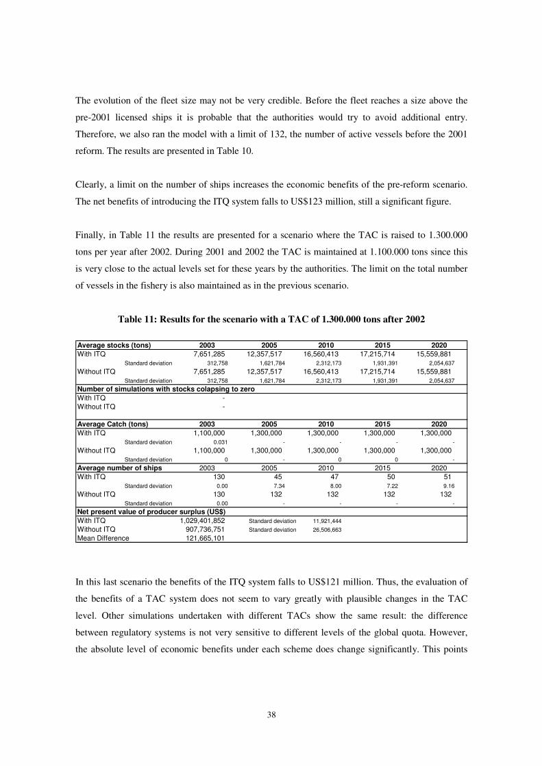
38

The evolution of the fleet size may not be very credible. Before the fleet reaches a size above the

pre-2001 licensed ships it is probable that the authorities would try to avoid additional entry.

Therefore, we also ran the model with a limit of 132, the number of active vessels before the 2001

reform. The results are presented in Table 10.

Clearly, a limit on the number of ships increases the economic benefits of the pre-reform scenario.

The net benefits of introducing the ITQ system falls to US$123 million, still a significant figure.

Finally, in Table 11 the results are presented for a scenario where the TAC is raised to 1.300.000

tons per year after 2002. During 2001 and 2002 the TAC is maintained at 1.100.000 tons since this

is very close to the actual levels set for these years by the authorities. The limit on the total number

of vessels in the fishery is also maintained as in the previous scenario.

Table 11: Results for the scenario with a TAC of 1.300.000 tons after 2002

In this last scenario the benefits of the ITQ system falls to US$121 million. Thus, the evaluation of

the benefits of a TAC system does not seem to vary greatly with plausible changes in the TAC

level. Other simulations undertaken with different TACs show the same result: the difference

between regulatory systems is not very sensitive to different levels of the global quota. However,

the absolute level of economic benefits under each scheme does change significantly. This points

Average stocks (tons) 2003 2005 2010 2015 2020With ITQ 7,651,285 12,357,517 16,560,413 17,215,714 15,559,881

Standard deviation 312,758 1,621,784 2,312,173 1,931,391 2,054,637

Without ITQ 7,651,285 12,357,517 16,560,413 17,215,714 15,559,881 Standard deviation 312,758 1,621,784 2,312,173 1,931,391 2,054,637

Number of simulations with stocks colapsing to zeroWith ITQ - Without ITQ -

Average Catch (tons) 2003 2005 2010 2015 2020With ITQ 1,100,000 1,300,000 1,300,000 1,300,000 1,300,000

Standard deviation 0.031 - - - - Without ITQ 1,100,000 1,300,000 1,300,000 1,300,000 1,300,000

Standard deviation 0 - 0 0 - Average number of ships 2003 2005 2010 2015 2020With ITQ 130 45 47 50 51

Standard deviation 0.00 7.34 8.00 7.22 9.16 Without ITQ 130 132 132 132 132

Standard deviation 0.00 - - - - Net present value of producer surplus (US$)With ITQ 1,029,401,852 Standard deviation 11,921,444 Without ITQ 907,736,751 Standard deviation 26,506,663

Mean Difference 121,665,101

39

out to the need of optimizing the TAC level in order to maximize the economic benefits from the

fishery. This is undertaken with this same model in an accompanying paper by the authors (Gómez-

Lobo, Barría and Peña-Torres, 2005).

6. Conclusions

An ITQ system was introduced in the southern pelagic fishery of Chile in 2001. This reform had an

immediate impact on the operation of the industrial fleet. The number of vessels active in the

fishery fell from 132 in 2000 to 65 in 2002. Among the benefits of reform are the lower capital and

operating costs of eliminating the chronic over investment that affected this fishery. In addition, the

elimination of the Olympic race also allowed fishermen to make a better planning of their

operations, giving them the option to decide whether or not to catch less fish in a given trip, thus

improving the average quality of landings and hence increasing the proportion of landings to be

allocated towards the higher value added segments of the industry.

In order to obtain a preliminary estimate of direct allocative efficiency benefits of the ITQ reform, a

bioeconomic model of the fishery capable of simulating the future behavior of biological and

economic variables under different regulatory systems is needed. To this end in this paper we used a

bioeconomic model estimated econometrically using past data of the fishery. This model reproduces

quite well the true evolution of key variables between 1987 and 2002. We use the model to simulate

several scenarios using Monte Carlo Techniques. The results indicate that the direct operational

benefits of the reform are substantial. The net present value of benefits varies between US$123 to

$366 million dollars between 2001 and 2020, depending on the particular assumptions used in each

scenario. This range of net present values implies a range of yearly net benefit gains which are

equivalent to between 6% - 19% of the total yearly exported value by the Chilean southern pelagic

fishery.

The way the ITQ system was introduced in Chile is also of interest. From December 1997 to

December 2000 the fishery was closed for biological reasons. However, the authorities organized

‘Experimental’ fishing expeditions in order to maintain the fleet active but under very controlled

operational conditions. These expeditions worked informally as a pseudo individual quota system.

This experience allowed fishermen to learn the benefits of such a system, which was instrumental in

facilitating the formal introduction of an ITQ system later. Perhaps this ‘didactic’ approach used in

Chile may be replicated in other countries wishing to introduce an ITQ system.

40

References

Barria, P. and R. Serra (1989), “Investigación Estimación Captura Total Permisible Sardina, año

1989”, Informe Técnico de Convenio Subsecretaría de Pesca e IFOP.

Begon, M. and M. Mortimer (1986), Population Ecology, 2nd ed., Blackwell Scientific Publications, Oxford.

Bjorndal, T., A-A Ussif and U.R. Sumaila (2004), ‘A Bioeconomic Analysis of the Norwegian

Spring Spawning Herring (NSSH) Stock’, Marine Resource Economics, vol. 19(3): 353-366

Clark, C. 1971. ‘Economically Optimal Policies for the Utilization of Biologically Renewable

Resources’, Mathematical Biosciences, Vol. 12: 245-260.

Clark, C. (1985), Bioeconomic Modelling and Fisheries Management, Wiley-Interscience

Publication, John Wiley & Sons, New York.

Dixit, A.K. and R.S. Pindyck (1994), Investment Under Uncertainty, Princeton University Press.

Gómez-Lobo, A., P. Barria, J. Peña-Torres and M. Basch (2004), ‘Modelo Bioeconómico de la

Pesquería Industrial Centro-Sur’, Informe de Avance, Proyecto Fondecyt Nº1020765, Santiago.

Gómez-Lobo, A., P. Barría and J. Peña-Torres (2005), ‘Optimal quotas for the Chilean Southern

Pelagic fishery’, mimeo.

Haddon, M. (2001), Modelling and Quantitative Methods in Fisheries, Chapman & Hall/CRC,

London.

Peña-Torres, J. and M. Basch (2000), “Harvesting in a Pelagic Fishery: The Case of Northern

Chile”, Annals of Operations Research vol. 94: 295-320.

Peña-Torres, J. (2002a), “Debates sobre Cuotas Individuales Transferibles: ¿“Privatizando” el mar?

¿Subsidios? O ¿Muerte anunciada de la pesca extractiva en Chile?”, Estudios Públicos, Nº86,

Otoño (Fall), pp. 183-222.

41

Peña-Torres, J. (2002b), “Individual Transferable Fishing Quotas in Chile: Recent History and

Current Debates”, Research Working Papers Series # I-139, Department of Economics,

Universidad Alberto Hurtado-ILADES, May.

Peña-Torres, J., M. Basch and S. Vergara (2003), “¿Eficiencia técnica y de escalas de operación en

pesca pelágica: un análisis de fronteras estocásticas”, Cuadernos de Economía, Vol. 40, Nº119

(April): 43-83.

Peña-Torres, J., S. Vergara and M. Basch (2004), “El dilema de la escala productiva frente a ciclos

de abundancia: la pesca industrial en Chile”, El Trimestre Económico, Nº283 (July-September):

575-612.

Sernapesca (2003), “Anuario estadístico de Pesca 2003”, Servicio Nacional de Pesca, Chile.

Yepes, M. (2004), “Dinámica Poblacional del Jurel: Reclutamiento Asociado a Factores

Ambientales y sus Efectos sobre la Captura”, Tesis para optar al grado de Master of Arts in

Economics Ilades-Georgetown University, Universidad Alberto Huratdo, Santiago, Diciembre.

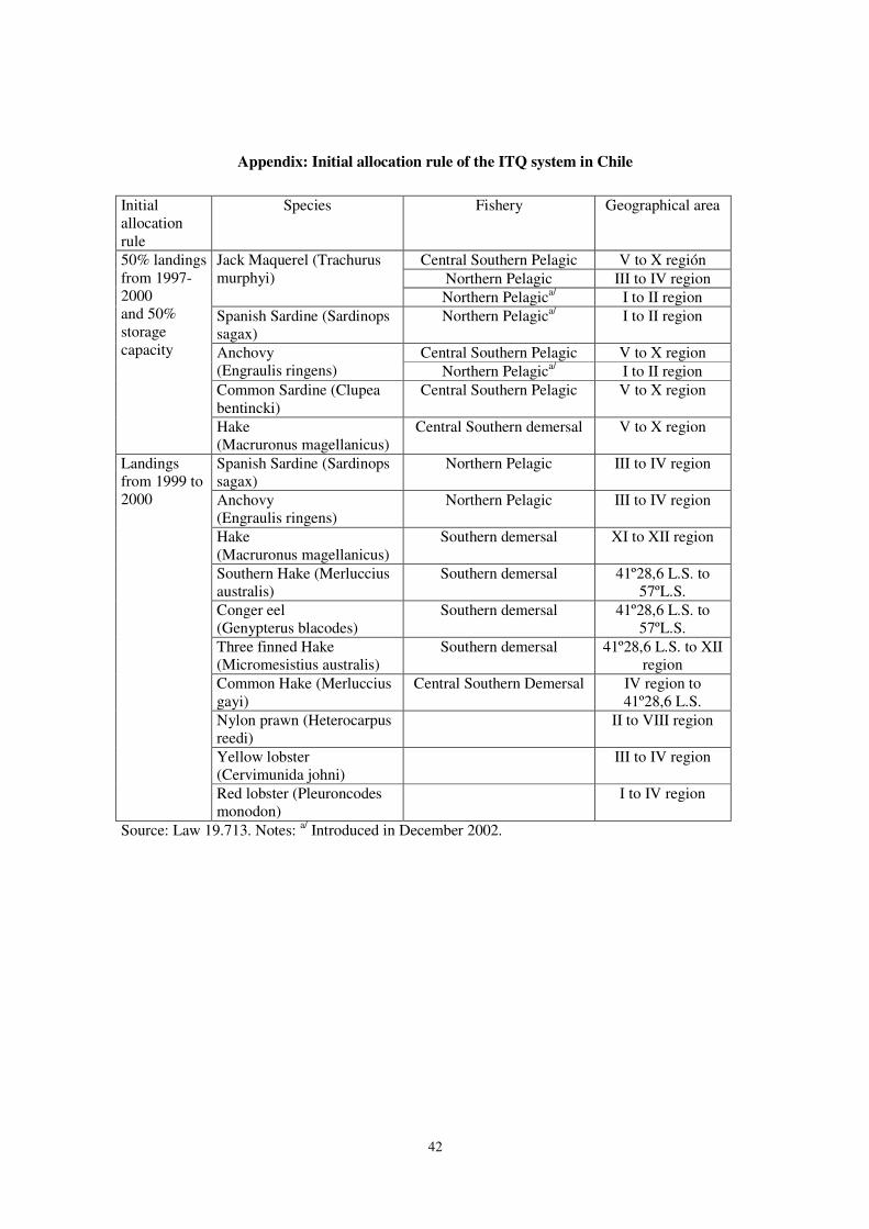
42

Appendix: Initial allocation rule of the ITQ system in Chile Initial allocation rule

Species Fishery Geographical area

Central Southern Pelagic V to X región Northern Pelagic III to IV region

Jack Maquerel (Trachurus murphyi)

Northern Pelagica/ I to II region Spanish Sardine (Sardinops sagax)

Northern Pelagica/ I to II region

Central Southern Pelagic V to X region Anchovy (Engraulis ringens) Northern Pelagica/ I to II region Common Sardine (Clupea bentincki)

Central Southern Pelagic V to X region

50% landings from 1997-2000 and 50% storage capacity

Hake (Macruronus magellanicus)

Central Southern demersal V to X region

Spanish Sardine (Sardinops sagax)

Northern Pelagic III to IV region

Anchovy (Engraulis ringens)

Northern Pelagic III to IV region

Hake (Macruronus magellanicus)

Southern demersal XI to XII region

Southern Hake (Merluccius australis)

Southern demersal 41º28,6 L.S. to 57ºL.S.

Conger eel (Genypterus blacodes)

Southern demersal 41º28,6 L.S. to 57ºL.S.

Three finned Hake (Micromesistius australis)

Southern demersal 41º28,6 L.S. to XII region

Common Hake (Merluccius gayi)

Central Southern Demersal IV region to 41º28,6 L.S.

Nylon prawn (Heterocarpus reedi)

II to VIII region

Yellow lobster (Cervimunida johni)

III to IV region

Landings from 1999 to 2000

Red lobster (Pleuroncodes monodon)

I to IV region

Source: Law 19.713. Notes: a/ Introduced in December 2002.