management and shocks to worker productivity · management and shocks to worker productivity ......

MANAGEMENT AND SHOCKS TO WORKER

PRODUCTIVITY∗

Achyuta Adhvaryu†

Namrata Kala‡

Anant Nyshadham§

May 9, 2016

Abstract

Differences in managerial quality likely contribute significantly to firm productivity gaps betweenfirms in developed and developing countries. But how specifically does management affect pro-ductivity? We model one potential channel for this effect: good managers are better able to dealwith shocks to worker productivity. We test the model’s predictions in an Indian garment factory,using hourly data on worker and line productivity, rich survey measures of managerial quality, andexogenous variation in pollution exposure, an important shock to worker effort. We find that linessupervised by higher quality managers (those better at identifying and solving production issuesin general, and those who specifically monitor production more frequently and are more likely toreplace underperforming workers) are more productive and exhibit more frequent reallocation ofworkers across tasks. We also find that productivity suffers in response to higher pollution ex-posure, and that the frequency of task reallocation rises as pollution deviates from median levels.Moreover, lines supervised by higher quality managers suffer substantially smaller losses in the faceof higher pollution exposure, by way of increased task reallocation. Finally, we validate our indicesof managerial quality against a measure of supervisor TFP, and provide descriptive evidence of thespecific practices, management styles, and personality traits that contribute to managerial quality.

Keywords: management, worker productivity, air pollution, ready-made garments, IndiaJEL Codes: L23, M11, O14

∗We thank Hunt Allcott, Manuela Angelucci, Nick Bloom, Dave Donaldson, Pascaline Dupas, Josh Graff Zivin, Ben Jones,Rocco Macchiavello, Aprajit Mahajan, Grant Miller, Melanie Morten, Dilip Mookherjee, Antoinette Schoar, John Strauss,Tavneet Suri, Chris Woodruff, Dean Yang, and seminar participants at USC, Stanford, Michigan, UIUC, Penn, Brown, UCSD,BC, BREAD, PEDL, and the NBER for comments and suggestions. We are incredibly thankful to Anant Ahuja, Chitra Ram-das, Shridatta Veera, Manju Rajesh, Raghuram Nayaka, Sudhakar Bheemarao, Paul Ouseph, and Subhash Tiwari for theircoordination, enthusiasm, support, and guidance. This research has benefited from support by the Private Enterprise De-velopment in Low-Income Countries (PEDL) initiative. Thanks to Tushar Bharati and Robert Fletcher for valuable researchassistance. Adhvaryu gratefully acknowledges funding from the NIH/NICHD (5K01HD071949). All errors are our own.†University of Michigan & NBER; [email protected]‡Harvard University & MIT Jameel Poverty Action Lab; [email protected]§Boston College; [email protected]

1

1 Introduction

Firms in poor countries are substantially less productive than firms in rich countries (Caselli, 2005;

Hall and Jones, 1999). Measurement of management practices across countries reveals that the spa-

tial distributions of productivity and the quality of management are strikingly similar (Bloom and

Van Reenen, 2007). Moreover, emerging evidence demonstrates that at least part of this relationship

is causal: improving managerial quality, at least in large firms, can generate considerable increases in

productivity (Bloom et al., 2013).

Still, we have limited evidence on the specific mechanisms that drive this impact. Some recent work

has begun to get inside the black box: Macchiavello et al. (2015) and Schoar (2014), for example, car-

ried out randomized management interventions in garment-producing firms that focused on technical

training and relationship management. In this study, we contribute evidence on a novel mechanism

for the impacts of management: good managers are better able to deal with shocks to worker produc-

tivity. We model the ability of managers to reorganize production in response to heterogeneous shocks

to their workers’ costs-of-effort. Good managers devote more attention (or equivalently, exert more

effort) toward monitoring their employees, and thus are able to make real-time adjustments to the al-

location of workers to tasks, which mitigates the impacts of shocks to individual productivity. This

mechanism fits into a growing literature on the consequences of managerial inattention (e.g., Ellison

and Snyder (2014); Reis (2006)).

We test the model’s predictions in the context of an Indian garment firm, using hourly data on

worker and line productivity, rich survey measures of managerial quality, and exogenous variation

in pollution exposure, an important shock to worker effort. We construct three indices of managerial

quality: a production problem-solving index, a worker monitoring and reallocation index, and a com-

bination of these two indices.1 We find that lines supervised by higher quality managers – those better

at identifying and solving production issues in general, and those who specifically monitor production

more frequently and are more likely to replace underperforming workers – are more productive and

exhibit more frequent reallocation of workers across tasks.

We also find that productivity suffers in response to higher pollution exposure, and that the fre-

quency of task reallocation rises as pollution deviates from median levels. Moreover, lines supervised

1Management data on practices, style, and personality were collected using survey instruments adapted from recent workon measuring managerial quality (Bloom and Van Reenen, 2007) as well as other standard personality and work historymodules.

2

by higher quality managers suffer substantially smaller losses in the face of higher pollution exposure,

by way of increased task reallocation. Finally, we validate our indices of managerial quality against

a measure of supervisor TFP, and provide descriptive evidence of the specific practices, management

styles, and personality traits that contribute to managerial quality. In sum, we show that one important

way in which managerial quality impacts productivity is through managers’ roles in diagnosing and

mitigating the deleterious impacts of worker productivity shocks.

This paper adds to a growing body of work in economics on the impacts of management (Bloom

et al., 2013; Bloom and Reenen, 2011; Bloom et al., 2010b; Bloom and Van Reenen, 2010; Bruhn et al.,

2010; Lazear et al., 2014; Schoar, 2014). We highlight an important but unexplored channel – managers’

responses to shocks to production – through which managerial quality impacts productivity in labor-

intensive manufacturing settings. This is made possible by the highly granular nature of our worker

productivity data and the collection of management quality measures at the lowest (and perhaps most

direct) level of production supervision.

We also contribute to the understanding of firm productivity in low-income countries (Bloom et al.,

2010a; Syverson, 2011; Tybout, 2000). Two branches of this literature are relevant to our study. First,

intra-firm barriers to productivity growth – such as ethnic and gender-related frictions (Hjort, 2014;

Macchiavello et al., 2015; Marx et al., 2015), information asymmetries (Heath, 2011), and the misalign-

ment of organizational incentives (Amodio and Martinez-Carrasco, 2015; Atkin et al., 2015) – are often

salient in low-income contexts. Second, environmental and infrastructural factors (which are often

tied to the environment) matter a great deal as well (Adhvaryu et al., 2015; Allcott et al., 2014; Dell

et al., 2012; Sudarshan and Tewari, 2013).2 We add to this literature estimates of the impacts of partic-

ulate matter pollution on worker productivity in a low-income country with pollution levels several

times higher than means in many high-income country environments. We estimate a negative gradi-

ent between air pollution and worker productivity using high-frequency micro-data, and find that this

gradient is steeper for more difficult tasks, consistent with evidence from the medical literature (e.g.,

Mills et al. (2005)).

The rest of the paper is organized as follows. Section 2 discusses the specific garment production

process in the study factory and reviews the medical evidence on the impacts of pollution exposure.

Section 3 develops a theoretical framework to formalize the role of management in responding to pro-

2A related literature focuses on the impacts of environmental factors on productivity and labor supply in more developedcountries. See, for example, Chang et al. (2014); Graff Zivin and Neidell (2012); Hanna and Oliva (2016).

3

ductivity shocks and outlines testable implications of the model. Then, section 4 discusses our data

sources and the construction of key variables and section 5 describes our strategy for empirically test-

ing the predictions of the model. Section 6 describes the results of these tests, and section 7 concludes.

2 Background

In this section, we discuss the garment sector in India, key elements of the garment production process

including the role of supervisors in determining productivity, and the physiological impacts of air

pollution exposure.

2.1 The Indian Garment Sector

Global apparel is one of the largest export sectors in the world, and vitally important for economic

growth in developing countries (Staritz, 2010). India is the world’s second largest producer of tex-

tile and garments, with export value totaling $10.7 billion in 2009-2010. With the steady transition of

the employment share in India, and in much of the developing world, from rural agricultural self-

employment to urban and peri-urban wage labor, the garment sector represents an unparalleled ca-

pacity to absorb this current and future influx of young, unskilled and semi-skilled labor (Heath and

Mobarak, 2015; World Bank, 2012). Furthermore, women comprise the majority of the global garment

workforce; and new labor force entrants tend to be disproportionately female in contexts like India

where the baseline female labor force participation rate is low (Staritz, 2010). Our research partner is

the largest private garment exporter in India, and the single largest employer of unskilled and semi-

skilled female labor in the country.

2.2 The Garment Production Process

There are three broad stages of garment production: cutting, sewing, and finishing. In this study, we

focus on sewing for three reasons. First, sewing makes up roughly 80% of the factory’s total employ-

ment. Second, a standardized measure of output is recorded for each worker in each hour on the

sewing floor. Third, the number of lines, and hence supervisors, is sufficiently large, and the mapping

of workers to supervisors is sufficiently dynamic (yet clearly observable), to allow for the study of the

interaction between supervisors and workers experiencing productivity shocks.

4

2.2.1 Cutting

Pieces of fabric needed for each segment of the garment are cut using patterns from a single sheet so

as to perfectly match color and fabric quality. These pieces are divided according to groups of sewing

operations (e.g. sleeve construction, collar attachment) and pieces for 10-20 garments are grouped and

tied into bundles. These bundles are then transported to the sewing floors where they are distributed

across the line at various “feeding points” for each group of sewing operations.

2.2.2 Sewing

Garments in this factory are sewn in production lines consisting of 50-150 workers (depending on the

complexity of the style) arranged in sequence and grouped in terms of segments of the garment (e.g.

sleeve, collar, placket). Roughly two-thirds to three-quarters of the workers on the line are machine

operators completing production tasks, while the remainder are helpers who are responsible for sup-

porting tasks such as folding, aligning and feeding. Each line produces a single style of garment at a

time (i.e. color and size will vary but the design of the style will be the same for every garment pro-

duced by that line until the sales order for that garment is met).3 Completed sections of garments pass

between machine operators, are attached to each other in additional operations along the way, and

emerge at the end of the line as a completed garment. These completed garments are then transferred

to the finishing floor.

2.2.3 Finishing

In finishing, garments are checked, ironed, and packed for shipping. Most quality checking is done

“in-line” on the sewing floor, but final checking occurs in the finishing stage. Any garments with

quality issues are sent back to the sewing floor for rework or, if irreparably ruined, are discarded

before packing. Orders are then packed and sent to port.

2.3 The Role of Supervisors

On the sewing floor, line supervisors play several important roles. First, due to absenteeism among

workers and the frequently changing demand for skills and efficiency derived from variation in gar-3In general, we describe here the process for woven garments; however, the steps are quite similar for knits and even

pants, with varying number and complexity of operations. Even within wovens, the production process can vary a bit bystyle or factory. The factory we are studying is a predominantly woven factory, and therefore, will follow the process outlinedhere very closely.

5

ment complexity, order sizes, and delivery dates and production timelines, the supervisors of each line

must adjust the worker composition of the line to optimize the garment-specific productivity subject

to continually evolving manpower constraints. Accordingly, on any given day, between 10 and 50% of

workers will be assigned to lines other than their usual production lines.

In addition to the worker composition of the line, the supervisor must also assign each worker to

a task or machine operation according to the perceived skill and speed of the worker and the com-

plexity of the task or operation. Then, during the production day, one of the main responsibilities of

the supervisor is to adjust this initial worker-task match to continually optimize performance based

on worker effort, shocks to capital, and the like. These adjustments, termed “line-balancing,” involve

switching the tasks to which workers are assigned, or increasing the number of workers on a particular

operation to shuffle more efficient workers to more complex tasks. Given the complex interrelation-

ships between the productivity of different workers on a given line, as well as the contribution of each

worker’s productivity to the total productivity of the line (which is of course the ultimate object of

concern for management), “line-balancing” is perhaps the most important mechanism by which fac-

tory management can respond to worker-specific productivity shocks, and is, therefore, an important

determinant of marginal productivity on the sewing floor.

2.4 Physiology of the Pollution-Productivity Gradient

A large body of studies connects particulate matter (PM) pollution to a host of morbidity and mortal-

ity impacts. Bell et al. (2004); Dockery and Pope (1994); Pope et al. (1999); Pope and Dockery (2006)

provide comprehensive literature reviews. There are three main categories of particulate matter based

on aerodynamic diameter range: coarse (greater than 2.5 micrometers (µm)), fine (less than or equal

to 2.5 µm), and ultra-fine (<0.1 µm). The focus in this study is on the second category, fine particulate

matter. Fine particulate matter has been shown to have the largest health impacts of the three, due

primarily to the following features: relative to larger particulates, they can be breathed more deeply

(Bell et al., 2004), remain suspended for a longer time and travel longer distances (Wilson and Suh,

1997), have a more harmful chemical composition, and penetrate indoor environments more easily

(Pope and Dockery, 2006).

Both long- and short-term exposures to particulate matter have impacts on health. Long-term

exposures have been linked to a variety of impacts, including mortality (see review articles above),

6

usually via elevated risk of cardiovascular events and chronic inflammatory lung injury (Souza et al.,

1998), which adversely affects the respiratory tract. Evidence form laboratory experiments confirm

that short-term exposures also cause elevated health risks. For instance, studies that have exposed

healthy human subjects to fine particulate matter for short periods in concentrations currently found

in polluted urban environments in the laboratory find evidence of adverse cardiovascular effects (Mills

et al., 2005), as well as acute vasoconstriction, which may also increase the probability of cardiac events

(Brook et al., 2002). Thus, both short- and long-term exposures to fine particulates impairs cardiac and

respiratory functioning in otherwise healthy adults.

3 Model

3.1 Setup

There are two tasks and two workers. Labor is indivisible, meaning a worker can only be devoted to

one task at a time. Let eik denote the effort given by worker i to task k.4

The output from task 1 (q1) is given as

q1 = h(ei1)

and the output from task 2 is given as,

q2 = g(q1, e2j) = g(ei1, ej2)

where subscript i, j denote the two workers and h′ > 0, h′′ < 0, h′′′ < 0, g1 > 0, g2 > 0, g11 < 0, g22 <

0, g111 < 0, g222 < 0, g12 > 0, g(0, e) = 0 ∀e. The final output Q is equal to q2. Note that conditional

on effort, output of each task does not depend on the identity of the worker. Also, because labor is

indivisible and q2 depends on q1, each task will be assigned one worker.

The worker’s problem

Now consider the workers problem. Worker i receives a benefit (wage) of b · qk where qk is the output

from the task which he is assigned.5 However, the worker experiences a disutility c(e + γiδ) from

4We focus on two workers and two tasks for simplicity of exposition but the results can be generalized to k > 2.5Though workers are paid a fixed base salary in our empirical context, they are eligible to earn daily production incentive

7

exerting effort e, with c′ > 0, c′′ > 0. Suppose without loss of generality that γ1 > γ2.6 This utility cost

depends in part on the level of a shock parameter δ, which is determined stochastically and is drawn

from the distribution F (δ) with E[δ] = 0. The worker observes (or, perhaps we should say “feels”) δ.7

Then given δ worker i assigned to task 1 solves

maxei1

bh(ei1)− c(ei1 + γiδ)

f.o.c.

bh′(ei1)− c′(ei1 + γiδ) = 0

s.o.c.

bh′′(ei1)− c′′(ei1 + γiδ) < 0

Since f is concave and and c is convex the second order condition holds. Worker i assigned to task 2

solves

maxei2

bg(ej1, ei2)− c(ei2 + γiδ)

f.o.c.

bg2(ej1, ei2)− c′(ei2 + γiδ) = 0

Thus solving the workers optimization problem we can solve for the workers optimal effort level

as a function of the shock parameter {(e∗11(δ), e∗12(δ)), (e∗21(δ), e∗22(δ)}.

The supervisor’s problem

The supervisor can choose the allocation of the tasks to each worker. He can choose between two

orderings g1 ≡ g(e11, e22) or g2 ≡ g(e21, e12). He is paid a fixed multiple of his line’s output, which for

simplicity we assume is 1 in the exposition below.8

bonuses. We abstract away from this feature of the employment contract and approximate the benefit to the worker as apiece rate for simplicity, but the main predictions of the theory are unaltered by this simplification.

6We omit the case γ1 = γ2 because all worker heterogeneity would be eliminated in this case.7We develop the model for a general shock-to-effort parameter, and test the model’s implications using high-frequency

variation in pollution levels as an empirical analog to this shock.8The supervisor’s contract in our empirical context is similar to the worker’s contract, which includes a base salary plus

daily bonus based on line production.

8

Perfect information benchmark

First consider the perfect information case (δ is known to the supervisor) as a benchmark. Then, given

δ the supervisor solves

g∗(δ) = max{g1(δ), g2(δ)}

The output of the line will equal g∗(δ).

Imperfect information

Now suppose that the supervisor can only observe δ if he pays a (disutility of effort) cost of monitoring,

denoted λ. If he chooses to not pay λ, then he will choose the ordering that maximizes output in

expectation. Thus he solves,

gE = max{Eg1, Eg2}

where Eg1 ≡∫g1(δ)dF (δ), and Eg2 ≡

∫g2(δ)dF (δ) respectively. Suppose that Eg2 < Eg1.

If, on the other hand, he does choose to expend the monitoring cost, then he observes δ and thus

chooses g∗(δ).

Given this setup, the supervisor will choose to monitor and expend λ iff

∫g∗(δ)dF (δ)− gE > λ

. We call a “good supervisor” someone with a monitoring cost small enough that he will possibly make

changes to line ordering based on observed levels of the shock parameter δ, i.e., λ < λ ≡∫g∗(δ)dF (δ)−

gE .

3.2 Testable Implications

We now turn to some analysis of comparative statics.

3.2.1 Output and Cost-of-effort Shocks

First, we elucidate the role of effort shocks in worker and supervisor decision-making.

Lemma 1. Task-specific individual effort level is decreasing in δ.

9

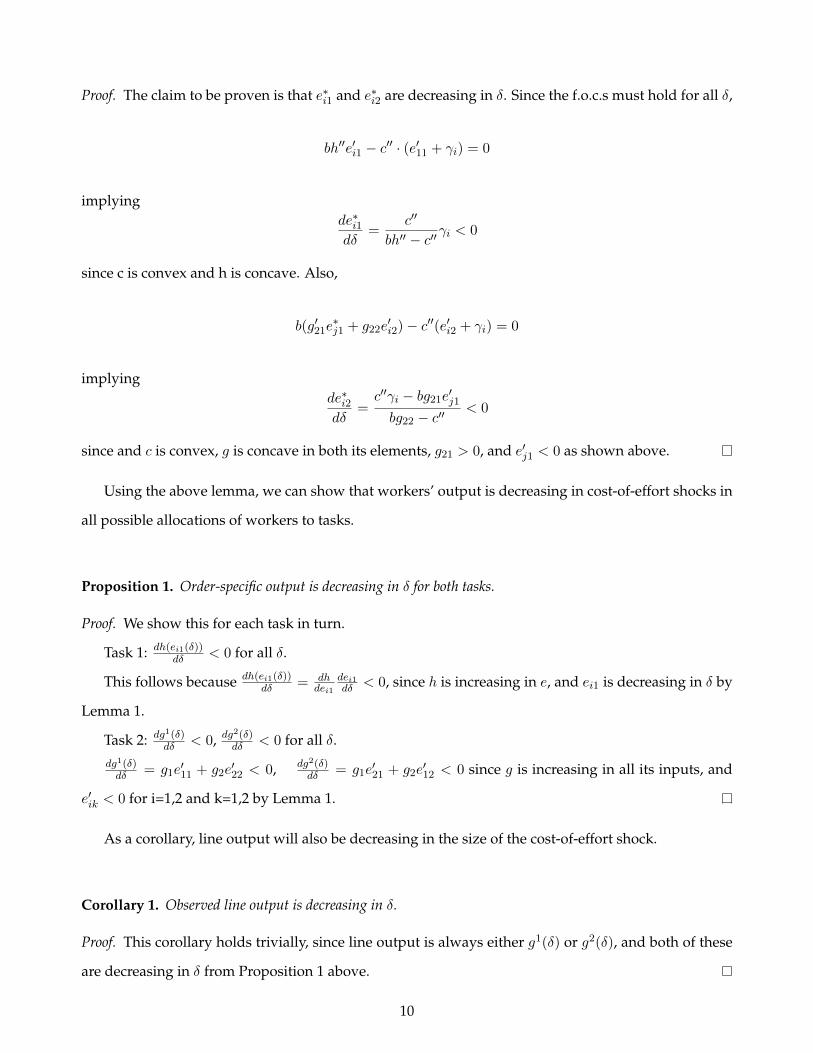
Proof. The claim to be proven is that e∗i1 and e∗i2 are decreasing in δ. Since the f.o.c.s must hold for all δ,

bh′′e′i1 − c′′ · (e′11 + γi) = 0

implyingde∗i1dδ

=c′′

bh′′ − c′′γi < 0

since c is convex and h is concave. Also,

b(g′21e∗j1 + g22e

′i2)− c′′(e′i2 + γi) = 0

implyingde∗i2dδ

=c′′γi − bg21e

′j1

bg22 − c′′< 0

since and c is convex, g is concave in both its elements, g21 > 0, and e′j1 < 0 as shown above.

Using the above lemma, we can show that workers’ output is decreasing in cost-of-effort shocks in

all possible allocations of workers to tasks.

Proposition 1. Order-specific output is decreasing in δ for both tasks.

Proof. We show this for each task in turn.

Task 1: dh(ei1(δ))dδ < 0 for all δ.

This follows because dh(ei1(δ))dδ = dh

dei1dei1dδ < 0, since h is increasing in e, and ei1 is decreasing in δ by

Lemma 1.

Task 2: dg1(δ)dδ < 0, dg

2(δ)dδ < 0 for all δ.

dg1(δ)dδ = g1e

′11 + g2e

′22 < 0, dg2(δ)

dδ = g1e′21 + g2e

′12 < 0 since g is increasing in all its inputs, and

e′ik < 0 for i=1,2 and k=1,2 by Lemma 1.

As a corollary, line output will also be decreasing in the size of the cost-of-effort shock.

Corollary 1. Observed line output is decreasing in δ.

Proof. This corollary holds trivially, since line output is always either g1(δ) or g2(δ), and both of these

are decreasing in δ from Proposition 1 above.

10

Next, we study how task “difficulty” prompts differential impacts of cost-of-effort shocks on indi-

vidual output. We embed task difficulty in the task-specific output functions. In particular, suppose

each unit produced is scaled by β ∈ (0, 1) in the worker’s maximization problems. That is, assume

each actual unit of production “counts for” β units. The closer to 0 is β, the more “difficult” a task is

said to be.9

To characterize the differential effects of more difficult tasks, we examine the responsiveness of

worker output to cost-of-effort shocks, studying comparative statics in this responsiveness with re-

spect to the difficulty parameter β. The following lemma establishes that optimal effort is increasing

in difficulty of the task.

Lemma 2. Worker effort is decreasing in task difficulty.

Proof. We show that ∂e∗i1

∂β > 0, and omit the analogous proof of ∂e∗i2

∂β > 0 for brevity.

Recall that the necessary first-order condition for ei1 is bβh′(e∗i1) = c′(e∗i1 + γiδ). Implicit differenti-

ation with respect to β (and suppressing subscripts) yields

b(h′(e) + βh′′∂e

∂β) = c′′

∂e

∂β. (1)

Rearranging terms, we obtain

∂e

∂β=

bh′

c′′ − βh′′b. (2)

The numerator of the above righthand-side expression is positive since h′ > 0, and the denominator

is also positive, since c′′ > 0 and h′′ < 0. Thus ∂e∗i1∂β > 0, as we set out to show.

For what follows, we assume that c′′′ ≈ 0, which would be the case, e.g., for any degree-two poly-

nomial cost of the form A1e2 +A2e+A3. We then get the following proposition regarding the linkage

between task difficulty and the responsiveness of output to cost-of-effort shocks.

Proposition 2. The (negative) impact of cost-of-effort shocks on task-specific output is increasing in task diffi-

culty.9This definition corresponds well to the industry-standard measure of “Standard Allowable Minutes,” which captures

(and standardize) the complexity of each task and garment.

11

Proof. We show that ∂2e∗i1∂δ∂β > 0. Again, we omit an analogous proof of ∂

2e∗i2∂δ∂β > 0 for brevity.

We begin with implicit differentiation of the necessary first-order condition for ei1 with respect to

δ. We obtain:

bβh′′(e∗i1)∂e∗i1∂δ

= c′′(e∗i1 + γiδ)(∂e∗i1∂δ

+ γi). (3)

Rearranging terms and suppressing subscripts, we get

∂e

∂δ=

c′′γ

bβh′′ − c′′(4)

Note that from above, ∂e∂δ < 0 since c′′ > 0 and h′′ < 0.

Next, we obtain ∂2e∂δ∂β by differentiating the above righthand-side expression with respect to β:

∂2e

∂δ∂β=γc′′′ ∂e∂β (bβh′′ − c′′)− c′′γ

(b(h′′ + βh′′′ ∂e∂β

)− c′′′ ∂e∂β

)(bβh′′ − c′′)2 . (5)

Since the sign of the above righthand-side expression only depends on the sign of the numerator

(the denominator is always positive), we turn our focus to the numerator. This expression can be

signed as follows:

γc′′′∂e

∂β

(bβh′′ − c′′

)︸︷︷︸

≈0

+−c′′γ︸︷︷︸<0

b(h′′ + βh′′′

∂e

∂β

)︸︷︷︸

<0

+−c′′′ ∂e∂β︸︷︷︸

≈0

> 0. (6)

This proves that ∂2e∗1∂δ∂β > 0, i.e., that the responsiveness of output to cost-of-effort shocks is increas-

ing in task difficulty.

3.2.2 Supervisor Behavior

Next, we consider supervisors’ decisions to allocate workers to tasks and how they change with cost-

of-effort shocks. In particular, we consider changes in the cost of effort occurring within an interval

around 0 with the property that shifting the cost of effort from one side of the interval to the other

changes the optimal allocation of workers to tasks. The following lemma shows the existence of this

interval.

12

Lemma 3. There exists (δ, δ) ∈ R− × R+ such that

∀δ ∈ (δ, 0), g2(δ) < g1(δ)

∀δ ∈ (0, δ), g1(δ) < g2(δ).

Proof. First note that if δ = 0, e∗11(0) = e∗21(0) and e∗12(0) = e∗22(0). This implies g1(0) = g2(0).

Claim: g′1(0) < g′2(0).

Since e∗11(0) = e∗21(0) and e∗12(0) = e∗22(0), I can denote g1 ≡ g1(e∗11(0), e∗22(0)) = g1(e∗21(0), e∗12(0))

and g2 ≡ g2(e∗11(0), e∗22(0)) = g2(e∗21(0), e∗12(0)). Recall g′1(δ) = dg1(δ)dδ = g1e

′11 + g2e

′22 and g′2(δ) =

dg2(δ)dδ = g1e

′21 + g2e

′12.

g′1(0)− g′2(0)

= g1(e′11 − e′21) + g2(e′22 − e′12)

= g1(e′11 − e′21) + g2(c′′γ2 − bg21e

′11

bg22 − c′′− c′′γ1 − bg21e

′21

bg22 − c′′)

=c′′

bg22 − c′′(g1(bg22 − c′′)− bg2g21)(

1

bh′′ − c′′− g2)(γ1 − γ2) < 0

Then since

(1) g′1(δ) < 0 and g′2(δ) < 0 for all δ,

(2) g′1(0) < g′2(0) < 0,

(3) g1(0) = g2(0),

and g1 and g2 are continuous in δ, there exists a δ > 0 such that g2 > g1 for all δ ∈ (0, δ). Similarly there

exists a δ < 0 such that g2 < g1 for all δ ∈ (δ, 0).

We consider implications for supervisor behavior of shifts between a “low” and a “high” level of

cost of effort–namely, between δL ∈ (δ, 0) and δH ∈ (0, δ), respectively. Examining this particular

comparative static is of interest because it lets us study what happens when the cost of effort shifts

enough that it changes the optimal worker-task ordering.

Table 1 categorizes the worker-task allocations of good and bad supervisors across these two levels

of cost of effort. It makes clear that bad supervisors, because they choose not to invest in monitoring

workers directly, do not switch worker ordering when the cost of effort shifts from δL to δH , keeping

13

δL δHBad supervisor (λ > λ) g1(δL) g1(δH)

Good supervisor (λ < λ) g1(δL) g2(δH)

Table 1: Worker-task allocations for good and bad supervisors across cost-of-effort shock levels

the ordering g1 regardless of the level of cost of effort. On the other hand, good supervisors always

invest in monitoring, and thus switch from g1 to g2 when the cost-of-effort shock parameter changes

from δL to δH , because g2 is optimal given δ = δH .

The following corollary follows directly from Table 1 and Lemma 3.

Corollary 2. Bad supervisors (λ > λ) always allocate workers to tasks following ordering g1. For δ ∈ (δ, 0),

good supervisors (λ > λ) choose g1, while for δ ∈ (0, δ), they choose g2.

Proof. By definition, supervisors for whom λ > λ never invest in monitoring, and thus choose to

allocate workers based on the expected output only, regardless of shock realizations. Thus, by the

assumption Eg1 > Eg2, bad supervisors always choose g1.

When λ < λ, supervisors always invest in monitoring, and thus allocate workers to tasks based on

realized levels of δ. By Lemma 3, the optimal allocation of workers to tasks follows g1 when δ ∈ (δ, 0),

but follows g2 when δ ∈ (0, δ).

Note that this corollary implies that increasing the cost-of-effort shock parameter (from δL to δH )

will induce good supervisors to switch line ordering, and decreasing this parameter (from δH to δL)

will induce switching for good supervisors, as well.

Next we study the repercussions of differential worker allocation by good and bad supervisors on

line output.

Proposition 3. Good supervisors have higher expected line output than bad supervisors on the interval (δ, δ).

Proof. We know that for δ ∈ (0, δ), g2(δ) > g1(δ). Thus,

∫ δ

δg1(δ)dF (δ) <

∫ 0

δg1(δ)dF (δ) +

∫ δ

0g2(δ)dF (δ). (7)

This proves the proposition.

14

Finally, we examine the extent to which good supervisors are able to mitigate fluctuations in output

occurring because of shifts in the cost-of-effort shock parameter.

Proposition 4. Consider an increase in δ from δL ∈ (δ, 0) to δH ∈ (0, δ). Both good and bad supervisors

experience decreases in output as a result of this increase in δ, but the reduction in output is smaller for good

supervisors.

Proof. Consider the change in output resulting from increasing δ from δL to δH :

Bad supervisors: g1(δH)− g1(δL) (8)

Good supervisors: g2(δH)− g1(δL). (9)

For bad supervisors, it is clear that g1(δH)− g1(δL) < 0, since g1 is decreasing in δ.

For good supervisors, note that g2(δH) < g2(δL) since g2 is decreasing in δ. Then, it follows that

g2(δH) − g1(δL) < g2(δL) − g1(δL) < 0. Thus output decreases for both good and bad supervisors

when the cost-of-effort shock rises from δL to δH . But note that since g2(δH) > g1(δH) by Lemma 3, the

change in output will be less negative for good supervisors. This proves what we set out to show.

Finally, we discuss the way in which switching worker ordering delivers bottleneck relief. Specifi-

cally, we decompose the effect of a change in line order on total output into 1) a direct effect of switch-

ing workers to different tasks, and 2) so-called bottleneck relief. The direct effect of workers on indi-

vidual tasks result from the workers’ differential costs of effort (sensitivity to cost-of-effort parameter),

and the indirect effects result from the complementarity of the workers’ effort levels, which can create

bottleneck effects.

To see this more clearly, consider the change in final output when changing the line order from g2

to g1. At this point we introduce some new notation. Given δ, let e∗ij ≡ e∗ij(δ), where i denotes worker

and j denotes task, and let ei2(e) denote worker i’s optimal effort level for task 2, when e is the effort

level of the worker assigned to task 1. Then for a given δ, the difference in production when switching

15

from g2 to g1 can be written as

g(e∗11(δ), e∗22(δ))− g(e∗21(δ), e∗12(δ))

= g(e∗21, e22(e∗21))− g(e∗21, e∗12)︸︷︷︸

worker effect on task 2

+ g(e∗11, e22(e∗21))− g(e∗21, e22(e∗21))︸︷︷︸worker effect on task 1

+ g(e∗11, e∗22))− g(e∗11, e22(e∗21))︸︷︷︸

bottleneck relief

(10)

The first component, labeled “worker effect on task 2”, denotes the change in output that would

occur if worker 2 was assigned to task 2 instead of worker 1, while the quantity of input q1 remains

unchanged. Thus it measures the individual effectiveness of worker 2 over worker 1 when matched

with task 2, holding all else equal.

The second component, labeled “worker effect on task 1”, measures the change in output that stems

from switching in worker 1 for worker 2 at task 1, holding the effort level exerted to task 2 constant

at the level described above. Thus this component measures the individual effectiveness of worker 1

over worker 2 when matched with task 1, holding all else equal.

The third component, labeled “bottleneck relief”, measures the increase in output that stems from

effort complementarity between the two tasks. It measures the output effect via the increase in effort

provided by worker 2 at task 2, as an optimal response to an increase in input 1 in the production of

the final good. In this sense, this effect can be interpreted as a bottleneck effect because, a low output

in the first task would induce a low level of effort by the worker assigned to task 2, hence creating a

“bottleneck” in the production process.

3.3 Summary of Predictions

Our model studies the effects of cost-of-effort shocks on worker productivity, and lays out one mecha-

nism through which good managers are able to blunt the impact of these shocks. In our model, good

supervisors are those who invest in closely monitoring their workers, and change the allocation of

workers to tasks on a production line in response to effort shocks. Optimal allocation varies with this

shock because workers experience the shock differently. As a result, good supervisors mitigate the

impacts of shocks on productivity by re-optimizing this allocation.

16

Below, we summarize each of the predictions discussed in the model, translating them into our

empirical context and reordering slightly to better fit the progression of the content that follows.

1. Good supervisors have higher line output on average than bad supervisors (Proposition 3).

2. Good supervisors monitor their workers and thus are more likely to make changes to line or-

dering; bad supervisors monitor less and thus are less likely to change line ordering (Corollary

2).

3. Worker and line output are decreasing in pollution (Proposition 1 and Corollary 1).

4. The impact of pollution on worker output is increasing task difficulty (Proposition 2).

5. Switching line ordering increases line output due to direct effects of differential effectivenesses

of task-matching and indirect effects stemming from relieving bottlenecks (Equation 10).

6. Good supervisors experience smaller decreases in line output than bad supervisors as a result of

pollution shocks (Proposition 4).

7. Large enough changes in pollution shift the optimal line ordering (Lemma 3).

8. Good supervisors make switches to line ordering in response to both increases and decreases in

pollution levels. Bad supervisors are less likely to switch line ordering in response to pollution

levels (Corollary 2).

4 Data

4.1 Pollution Data

The air pollution data used in this study were collected using 5 particulate matter monitors positioned

at different locations across the 2 sewing floors of the garment factory.10 Two monitors were placed

on the first floor on which lines 1 through 9, along with an occasional line 10, are located; and the

remaining three monitors were placed on the second floor on which lines 11 through 17 are located.

We average across monitors within floor, for two reasons: 1) within floor correlation across monitors

is very high, and 2) some observations are missing for some monitors for some hours on some days

10The monitors used were custom calibrated particulate matter count monitors from the Dylos Corporation.

17

(most likely due to power continuity issues). Taking within floor averages for hourly observations

maximizes the number of non-missing observations without substantial loss to identifying variation

in the pollution measures.

The monitors were calibrated to collect two distinct counts of particulates: 1) those between 0.5-2.5

microns in diameter (fine particulates), and 2) those between 2.5 and 10 microns in diameter (coarse

particulates). In the analysis that follows, we focus on the impacts of fine particulate matter (PM)

on efficiency controlling for coarse PM. We do so because fine PM is unlikely to be produced by the

garment production activities on the sewing floor, but rather is due to ambient air pollution, namely

industrial combustion and automobile exhaust. On the other hand, coarse PM is produced by the

garment production process and could therefore exhibit reverse causality: high efficiency produces

high coarse PM levels. Lastly, as previously discussed, the environmental and medical literatures

suggest that fine PM is the more impactful of the two particulates due to its ability to accumulate in

the lungs and restrict respiration.

4.1.1 Fine Particulates (PM 2.5)

We can check the exogeneity of fine PM levels by studying whether fine PM levels decay at the end

of the work day and work week when production stops, and how this decay compares to coarse PM

which we hypothesize is endogenous to production.11

Figure 1A

050

100

150

Fine

PM

Jan

Feb

Mar Ap

r

May Jun Jul

Aug

Sep

Oct

Nov

Dec

Month

Mean SD

Figure 1B

020

4060

8010

0Fi

ne P

M

Sund

ay

Mon

day

Tues

day

Wed

nesd

ay

Thur

sday

Frid

ay

Satu

rday

Day of Week

Mean SD

Figure 1C

2040

6080

100

Fine

PM

9AM

10AM

11AM

12PM 1P

M

2PM

3PM

4PM

5PM

Production Hour

Mean SD

Figures 1A-1C depict means and standard deviations of fine particulate matter within each month, day of the week, andhour of the day, respectively. Note that June and July do not appear in our dataset; Sundays are non-production days; andproduction hours are between 9am and 5pm.

11Lastly, it is clear that to the degree that fine PM is in fact produced by the manufacturing process, this reverse causalitywill bias estimates of the negative impact of fine PM exposure on worker productivity towards zero.

18

As shown in Figures 1A-1C, fine PM levels vary systematically by month or season of the year, as

well as day of week and hour of the day. Specifically, fine PM levels tend to be highest on average

in the winter months, later in the week, and at the beginning of the production day. These patterns

likely reflect the burning of carbon-based fuels for heating and industrial energy demand as well as

automobile traffic patterns. The PM data used in this study are from August 2013 through early May

2014.

4.2 Production Data

Production data were collected using tablet computers assigned to each production line on the sewing

floor. Each production writer (traditionally charged with recording by hand on paper each machine

operator’s completed operations each hour for the line), was trained to input production data directly

in the tablet computer. These inputs were then transmitted directly into the firms administrative data

servers via wireless network connection.

4.2.1 Productivity

The key measures of worker and line productivity we study below are pieces produced and efficiency.

At the worker-hour level, pieces produced are simply the number of garments that passed a worker’s

station by the end of that production hour. For example, if the worker’s operation were to sew plackets

onto shirt fronts, the number of shirt fronts that had plackets attached by the end of a given production

hour would be recorded as that worker’s “pieces produced.” In order to calculate line-level hourly

production from these worker-hour observations, we average the pieces produced by each worker on

a production line in a given production hour. This is the most appropriate measure in that it most

correctly accounts for partially completed garments at stations along the line in a given hour.

Efficiency is calculated as pieces produced divided by the target quantity of pieces per unit time

(in this case, hour). The target quantity for a given garment is calculated using a measure of garment

complexity called the standard allowable minute (SAM). SAM is defined as the number of minutes

that should be required for a single garment of a particular style to be produced. That is, a garment

style with a SAM of .5 is deemed to take a half minute to produce one complete garment.12 SAM, as

the name denotes, is standardized across the global garment industry and is drawn from an industrial

12A SAM of .5 is not unlikely. The mean of SAM across worker hourly observations is .61 and its standard deviation is .20.

19

engineering database. However, this measure may be amended to account for stylistic variations from

the representative garment style in the database. Any amendments are explored and suggested by

the sampling department, in which master tailors make samples for costing purposes of each specific

style to be produced by lines on the sewing floor. The target quantity for a given unit of time for a

line producing a particular style is then calculated as the unit of time in minutes divided by the SAM.

That is, the target quantity to be produced by a line in an hour for a style with a SAM of .5 will be

60/.5 = 120.

Figure 2A

3040

5060

70M

ean

Effic

ienc

y

2040

6080

Mea

n Pi

eces

Pro

duce

d

Jan

Feb

Mar Ap

r

May Jun Jul

Aug

Sep

Oct

Nov

Dec

Month of Year

Pieces Mean Pieces SDEfficiency Mean Efficiency SD

Figure 2B

3040

5060

70M

ean

Effic

ienc

y

3040

5060

70M

ean

Piec

es P

rodu

ced

Mon

day

Tues

day

Wed

nesd

ay

Thur

sday

Frid

ay

Satu

rday

Day of Week


Figure 2C

3040

5060

70M

ean

Effic

ienc

y

3040

5060

70M

ean

Piec

es P

rodu

ced

9AM

10AM

11AM

12PM 2P

M

3PM

4PM

5PM

Hour of Day


Figures 2A-2C depict means and standard deviations of efficiency (left y-axis) and pieces produced (right y-axis) within eachmonth, day of the week, and hour of the day, respectively. Note that June and July do not appear in our dataset; Sundays arenon-production days; and production hours are between 9am and 5pm.

As shown in Figures 2A-2C, productivity also follows mild seasonal and hour-of-day patterns.

Specifically, productivity peaks around March with late winter and early spring showing high produc-

tivity, as well. These patterns line up with the seasonal global demand in the ready-made garments

industry. Productivity trends upwards through the first 3-4 hours of the day before plateauing.

These patterns appear somewhat coincident with the patterns in fine PM and might convolute the

analysis of causal impacts of fine PM on productivity and other work outcomes. Accordingly, we will

restrict our attention in the ensuing analysis to comparisons within month, day-of-week, and hour-of-

day.

4.2.2 Task Match Adjustments

The other main outcome measure we use in the empirical analysis is a dummy for any task match

adjustment on the line. Specifically, we first define “task match adjustment” as the reassignment of a

20

worker to a different operation from the operation she was doing in the last production hour. That

is, if a worker is doing a different operation this hour than last, we code the task match adjustment

dummy variable as a 1, and code a 0 if they are doing the same operation as in the last hour. We ignore

operation changes across days and reassignment of workers across lines as these are primarily driven

by manpower fluctuations rather than worker-specific productivity issues.

We then construct the line-level task match adjustment measure we use in the analysis from these

worker-hour task match adjustment measures. Any Task Match Adjustment is a binary variable taking

the value 1 if any worker on a line has been moved to a different operation this hour than the operation

they were doing last production hour, and 0 otherwise. That is, it is the maximum value across workers

on the line of the worker-hour task match adjustment measure discussed above.

4.3 Management Survey Data

In order to assess managerial quality, we surveyed production line supervisors in the factory, mea-

suring demographic characteristics, managerial practices, managerial skills, and personality traits. We

drew from several sources to construct the management questionnaire, in particular borrowing heav-

ily from Bloom and Van Reenen (2010) to construct instruments measuring management practices,

skills, and styles. We assemble two indices out of five variables that most closely measure the notion

of managerial quality and effort discussed in section 3 above.

The Production Problem Solving Index is constructed from three variables: 1) a dummy variable for

whether the line supervisor reports that he generally learns about production issues from talking to

workers on the line, 2) a dummy variable for whether the line supervisor is fluent in the native lan-

guage of the majority of the workers on the line, and 3) a dummy variable for whether the supervisor

reports generally solving production issues on his own without having to consult others. There are

between 1 and 3 supervisors assigned permanently to each line. These supervisors are not necessarily

responsible for subsets of workers or operations, but are collectively responsible for the total line. Ac-

cordingly, the dummies are then averaged across all supervisors assigned to the line, and the index is

a simple sum of these three averaged dummies, taking values of 0 to 3. This index is meant to measure

in a general sense the degree to which the manager is able to detect and solve production issues.

The Monitoring and Reallocation Index is constructed from two variables: 1) a dummy variable for

whether the supervisor reported making rounds of the line to monitor production at least every 10

21

min (which was the highest possible frequency response) , and 2) a dummy variable for whether the

supervisor reported that they would try to replace a worker that was performing poorly. In translating

these variables to the line level, we construct a dummy for whether all supervisors of a line reported

monitoring at least every 10 minutes, and calculate the average across supervisors of a line for the

worker replacement variable as a measure of the probability that an underperforming worker is re-

placed. The index is then a simple sum of these two variables, taking values of 0 to 2, and is meant to

measure the degree to which managers engage in the specific activities modeled as evidence of higher

effort or quality in section 3 above. Lastly, we construct a Composite Index which is simply the sum of

the Production Problem Solving Index and the Monitoring and Reallocation Index, taking values 0 to 5.

Finally, we also utilize variables measuring specific managerial practices, management style, and

personality traits in descriptive regressions aimed at unpacking the information contained in the in-

dices discussed above. For managerial practices, we focus on which specific activities the supervisor

reports engaging in to ensure that production targets are met. These include making rounds of the line

and discussing targets with workers among other activities. We construct a mean effect measure from

individual binary variables for each of these activities. We construct analogous mean effect measures

for activities related to reinforcing high level performance from star workers (e.g., acknowledging high

performance in front of other workers, recommending star performers for promotions) and for activ-

ities related to retaining high performing workers (e.g., talk to worker directly to convince them to

stay, recommend a salary increase). For management style, we construct two analogous mean effect

measures: 1) positive leadership behavior (e.g., give advance notice of changes, back up the workers

on line, explain my actions); and 2) passive conflict resolution (e.g., direct reports resisted initiatives,

had interpersonal conflicts with direct reports). We also construct four mean effects measures from

standard psychological modules on personality: in particular, conscientiousness, locus of control, per-

severance, and self-esteem. Further detail regarding these measures is given in the Data Appendix.

4.4 Summary Statistics

Table 2 presents summary statistics of the main variables of interest. Fine PM in the pooled sample

is roughly 51, with a standard deviation of roughly 26. The units of fine PM have been translated

as closely as possible to µg/m3 in order to allow for easy comparison with impacts from previous

studies.13 Pieces produced and efficiency both have means of roughly 50. Task Match Adjustment13For the sake of comparison, the mean level of fine particulates in Southern CA is 10- 20 µg/m3.

22

Table 2: Summary Statistics

Number of observations

Number of days

Number of workers

Number of lines

Number of Line Supervisors

Mean SD Mean SD Mean SD

Pollution Fine PM 51.47597 26.52471 51.32857 26.11829 51.31172 26.05516 Coarse PM 624.1194 217.1332 622.1406 214.5416 611.5284 209.0065

Production Pieces Produced 50.59853 22.39275 49.56163 15.76222 50.37713 16.44089 Hourly Efficiency 49.14378 21.12376 48.22987 14.1346 48.81886 14.53656

Task Match Adjustment Any Task Match Adjustment 0.4181425 0.493271 0.4154 0.4928115 Pct of Workers Reallocated 1.235551 2.07021 1.194546 2.01871

Managerial Quality Indices Production Problem Solving Index 2.067841 0.9381541 Monitoring and Reallocation Index 1.567326 0.391975 Composite Index 3.635168 1.152347

Table 1Summary Statistics

(3)

17

-

-

210

Supervisor Line-Hour Sample

11,974

(1)Worker-Hour Sample

1,054,962

(2)Line-Hour Sample

14,342

13

Notes: The units of fine PM have been translated as closely as possible to micrograms per cubic meter in order to allow for easy comparison with impacts from previous studies. Coarse PM units are raw particle counts per measurement. Efficiency is defined as pieces produced over target pieces. Production Problem Solving Index is constructed from three variables: 1) a dummy variable for whether the line supervisor reports that he generally learns about production issues from talking to workers on the line, 2) a dummy variable for whether the line supervisor is fluent in the native language of the majority of the workers on the line, and 3) a dummy variable for whether the supervisor reports generally solving production issues on his own without having to consult others. There are between 1 and 3 supervisors assigned permanently to each line. These supervisors are not necessarily responsible for subsets of workers or operations, but are collectively responsible for the total line. Accordingly, the dummies are then averaged across all supervisors assigned to the line, and the index is a simple sum of these three averaged dummies, taking values of 0 to 3. This index is meant to measure in a general sense the degree to which the manager is able to detect and solve production issues. Monitoring and Reallocation Index is constructed from two variables: 1) a dummy variable for whether the supervisor reported making rounds of the line to monitor production at least every 10 min (which was the highest possible frequency response) , and 2) a dummy variable for whether the supervisor reported that they would try to replace a worker that was performing poorly. We take the minimum value across the supervisors of the line for the monitoring dummy since the majority of supervisors reported monitoring every 10 min. We do this to maximize the amount of variation in this variable. We average the second dummy as responses were more balanced to this question. The index is a simple sum of these two variables, taking values of 0 to 2, and is meant to measure the degree to which managers engage in the specific activities modeled as products of higher effort or quality in the model. Composite Index is simply the sum of the Production Problem Solving Index and the Monitoring and Reallocation Index, taking values 0 to 5.

-

210

24

17

-

1750

210

23

is quite common, with over 40% of line-hour observations reporting at least one worker reassigned.

However, a small percentage of workers on the line are reassigned on average: only 1.2% of workers on

the line are reassigned, or less than 3% conditional on any task match adjustment. With an average of

just under 82 workers per line in a given hour, the average line thus sees about 2.5 workers reallocated

per hour.

5 Empirical Strategy

5.1 Overview

The empirical analysis proceeds in several steps, following the model summary in section 3. We first

estimate the degree to which average line productivity varies by managerial quality. We do this by

regressing line productivity measures on the different managerial indices we have constructed, along

with an appropriate set of controls to account for the coincident patterns over time in pollution and

productivity discussed in section 4. We later estimate the degree to which average task match adjust-

ment on the line varies by managerial quality in much the same way.

Next, we estimate the impact of pollution (fine PM) on both worker and line level productivity

measures, controlling for contemporaneous coarse PM levels and month, day-of-week, and hour-of-

day fixed effects. We then estimate the degree to which this impact varies by task difficulty (as mea-

sured by SAM), and by position in the line (the so-called “seat in line”). These heterogenous impacts

of pollution on worker-task productivity are also predicted by the model and, if verified empirically,

would help to validate the appropriateness of the model for our empirical context. Most importantly,

we estimate the degree to which the impact of pollution varies by managerial quality.

Finally, we estimate the reallocation response to pollution exposure (or more specifically, deviations

from “usual” pollution levels) and the degree to which these responses vary by managerial quality. We

conclude by estimating partial correlations between managerial quality and specific practices, style,

and personality traits in order to unpack the determinants of our indices.

24

5.2 Specifications

We estimate the following managerial quality specification for productivity of line l in hour h on day

of the week d in month m and year y:

Plhdmy = α0 + ζMl + βFPMfhdmy + φCPMfhdmy + ψy + γh + ηm + δd + εlhdmy (11)

Here, ζ is the coefficient of interest, measuring the relationship between managerial quality and

line productivity. As discussed in section 4, Ml represents one of 3 managerial indices: Production

Problem Solving Index, Monitoring and Reallocation Index, and Composite Index. Also as discussed

in section 4, we use both pieces produced and efficiency as measures of line level productivity. FPM

is fine PM and CPM is coarse PM on floor f for hour h on day d in month m and year y.14 γh are hour

fixed effects; ψy are year fixed effects; ηm are month fixed effects; and δd are day-of-week fixed effects.

εlhdmy is an error term.15 In all specifications with pieces produced as the outcome, we include target

pieces as an additional control. We do not need this control when using efficiency as the outcome,

since target pieces is already in the denominator of efficiency. This control accounts for variation in

productivity due to the complexity of the garment.

We include this control in specifications of pieces produced below as well. We then estimate spec-

ifications in which we replace productivity outcomes Plhdmy with the task match adjustment outcome

Rlhdmy. When doing so we replace linear pollution controls FPM and CPM with above and below-

median linear splines to account for the non-monotonic relationship between pollution and task match

adjustment predicted by the theory.

We estimate the following pollution specification for the productivity of worker i in hour h on day

14Although we collected simultaneous pollution measurements from 5 monitors across the 2 production floors (i.e., 3 onone floor and 2 on the other), some measurements are missing for some hours on some days. The measurements are alsovery highly correlated within floor. Accordingly, we average across non-missing measurements for each floor to minimize thenumber of missing values. We have run results using both raw individual measurements from each monitor and averagingacross both floors and find qualitatively identical results.

15Although we believe these errors to be close to i.i.d across worker-hour observations after conditioning on the full setof time fixed effects, we want to be conservative in allowing for errors to be correlated within production line given thatin these basic specifications the regressor of interest varies at only the production line level. Accordingly, we report line-specific random effect robust errors as our main standard errors in estimates from this specification to allow for errors tobe equicorrelated within line. In all more complex specifications below in which pollution measures and interactions withpollution are our main regressors of interest, we report errors clustered at the hour by date level since these regressors varyat that level. We, however, report additional more conservative estimated standard errors in appendix tables to demonstrateadditional robusntess, but believe these models to be less appropriate for our empirical context.

25

of the week d in month m and year y:

Pihdmy = α0 + βFPMfhdmy + φCPMfhdmy + ψy + γh + ηm + δd + εihdmy (12)

Here, β is the main coefficient of interest, measuring the impact of exposure to fine particulate

matter level, FPM , on floor f for hour h on day d in month m on worker hourly productivity P . Error

εihdmy is assumed i.i.d. conditional on hour of the day x date. That is, errors are clustered at the hour

by date level. This is the appropriate level of clustering given that the regressor of interest (fine PM)

varies at the hour by date level. We estimate equation 12 at the line level as well, as the model predicts

impacts of pollution on both worker and line level productivity. CPM is coarse PM on floor f for hour

h on day d in month m. γh are hour fixed effects; ψy are year fixed effects; ηm are month fixed effects;

and δd are day-of-week fixed effects.

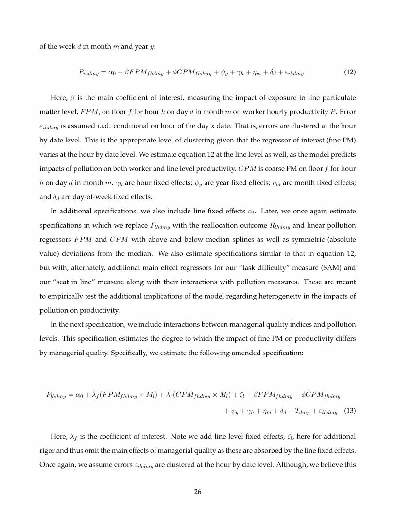
In additional specifications, we also include line fixed effects αl. Later, we once again estimate

specifications in which we replace Plhdmy with the reallocation outcome Rlhdmy and linear pollution

regressors FPM and CPM with above and below median splines as well as symmetric (absolute

value) deviations from the median. We also estimate specifications similar to that in equation 12,

but with, alternately, additional main effect regressors for our “task difficulty” measure (SAM) and

our “seat in line” measure along with their interactions with pollution measures. These are meant

to empirically test the additional implications of the model regarding heterogeneity in the impacts of

pollution on productivity.

In the next specification, we include interactions between managerial quality indices and pollution

levels. This specification estimates the degree to which the impact of fine PM on productivity differs

by managerial quality. Specifically, we estimate the following amended specification:

Plhdmy = α0 + λf (FPMfhdmy ×Ml) + λc(CPMfhdmy ×Ml) + ζl + βFPMfhdmy + φCPMfhdmy

+ ψy + γh + ηm + δd + Tdmy + εlhdmy (13)

Here, λf is the coefficient of interest. Note we add line level fixed effects, ζl, here for additional

rigor and thus omit the main effects of managerial quality as these are absorbed by the line fixed effects.

Once again, we assume errors εihdmy are clustered at the hour by date level. Although, we believe this

26

is the appropriate error structure to impose, we explore robustness to relaxing this assumption to allow

for two types of within-line correlation in the errors in Tables A3 and A4 of the Appendix. Next, to

explore the mechanisms driving these heterogeneous productivity impacts of pollution by managerial

quality, we also re-estimate equation 13 replacing outcome Plhdmy with Rlhdmy and pollution measures

FPM and CPM with, alternately, above and below median splines and symmetric (absolute value)

deviations from the median in both the main effect and interaction terms.

Finally, we validate the managerial quality index results by reestimating the reallocation version

of equation 13 but with the addition of a supervisor residual TFP measure as an alternate measure of

managerial quality; and then attempt to decompose managerial quality into specific practices, style,

and personality measures. We do this by first estimating a worker level log production function (i.e.,

ln(pieces produced) on time fixed effects from the main specification and worker fixed effects to ac-

count for individual worker contributions to output) and constructing average line level predicted

residual measures. These line averaged predicted residuals reflect, among perhaps other determinants,

supervisor contributions to output; we, accordingly, call these supervisor residual TFP measures.16

We construct a dummy for above median supervisor TFP residual from these measures and esti-

mate specifications similar to equation 13 with Rlhdmy as the outcome, spline and absolute deviation

from median pollution regressors, and additional terms for the interaction of above median supervi-

sor residual TFP with the pollution measures.17 We then regress the constructed supervisor residual

TFP measure on the managerial quality indices to investigate their partial correlations. We finish by

regressing each of the managerial quality indices and the constructed supervisor residual TFP measure

on additional measures from the management survey we conducted. These additional measures re-

flect specific management practices, management style, and personality traits and help to decompose

the information contained in the managerial indices used in the main regressions.

16Note that this specification matches a log-linearized Cobb-Douglas production function with each worker as an input andthe regression coefficient on them as the marginal productivity i.e. the production function is given by Y = At(L

b11 ...L

bkk ),

with At = e(csDs+atDt), where Ds is the supervisor’s contribution to production, cs is the factor load on the supervisor’scontribution, Dt are the time dummy variables, and ct is the vector of factor loads on the time dummy variables. The log-linear version of this production function is thus given by ln(Y ) = γh + ψy + ηm + δd + κw + ε, where γh, ψy, ηm, and δdare time fixed effects (hour of the day, year, month, and day of the week fixed effects, respectively), κw are worker fixedeffects, and the mean of the residual ε at the line level is the supervisor contribution to production cs (the supervisor TFPresidual measure). It should be made clear that the outcome in this regression (i.e., ln(pieces produced)) differs from ourusual outcome (i.e., pieces produced in levels) because the previous regressions are meant to provide results of reduced formtests of implications from the model in which we did not impose any particular functional form (unlike the Cobb-Douglasform imposed here to recover production function residual TFP of the supervisor). This strategy is similar to Bloom et al.(2012) in that the objective is to compare how management measures are related to the TFP residual, but the procedure itselfis most similar to that of Stolarick et al. (1999), since that is the most appropriate way to map productivity net of other factorsto supervisors in our setting.

17Note main effects of supervisor residual TFP is absorbed by line fixed effects.

27

Table 3: Managerial Quality and Line Productivity

(1) (2) (3) (4) (5) (6)

Production Problem Solving Index 3.15390*** 3.04921***

(0.12960) (0.12109)

Monitoring and Reallocation Index 2.83950*** 2.91093***

(0.30630) (0.29667)

Composite Index 2.33202*** 2.30863***

(0.10347) (0.09787)

Production Target

Fine and Coarse PM Controls

Year, Month, Day-of-Week, Hour-of-Day FE Yes Yes Yes Yes Yes Yes

Observations 11,974 11,974 11,974 11,974 11,974 11,974

Mean of Dependent Variable

Table 2

Managerial Quality and Line Productivity

Notes: Robust standard errors in parentheses (*** p<0.01, ** p<0.05, * p<0.1). The errors reported are random effects errors which allow for equicorrelated errors within line.

Efficiency

mean(pieces produced / target pieces)

Pieces Produced

mean(pieces produced by workers on line within hour)

50.38 48.82

Linear

Control Regressor Outcome Denominator

6 Results

6.1 Managerial Quality and Production

We begin in Table 3 by presenting results from the estimation of equation 11. Estimates correspond

to coefficient(s) of interest ζ in equation 11. As described in the theory, lines managed by supervisors

of higher managerial quality should achieve higher expected line output. Indeed, we find across all

specifications that higher managerial quality as measured by each of the managerial indices predicts

higher productivity, both in terms of mean pieces produced by workers on the line in an hour and mean

efficiency. Specifically, we find that a one unit increase in each of the indices leads to a higher expected

output of roughly between 2.3 and 3.2 pieces produced per hour or between 2.3 and 3 percentage points

in efficiency. These coefficients represent an increase of around 6% of the means of these productivity

outcomes for each 1 unit change in these indices. As shown in Table 2, a one unit change is roughly

a standard deviation of both the Production Problem Solving Index and Composite Index and roughly 2.5

standard deviations in the Monitoring and Reallocation Index.

6.2 Managerial Quality and Task Reallocation

Next, we estimate equation 11 with task match adjustment as the outcome (and pollution controls

adjusted appropriately). These estimates are reported in Table 4 and once again validate the model

28

Table 4: Managerial Quality and Task Match Adjustments

(1) (2) (3)

Production Problem Solving Index 0.01256**(0.00483)

Monitoring and Reallocation Index 0.14737***(0.01148)

Composite Index 0.02497***(0.00389)

Fine and Coarse PM ControlsYear, Month, Day-of-Week, Hour-of-Day FE Yes Yes Yes

Observations 11,974 11,974 11,974Mean of Dependent Variable

Table 3Managerial Quality and Task Match Adjustment

0.42

Notes: Robust standard errors in parentheses (*** p<0.01, ** p<0.05, * p<0.1). The errors reported are random effects errors which allow for equicorrelated errors within line.

Any Task Match Adjustment1(at least one worker on line reassigned to a different task this hour

from last hour)

Above and Below Median Absolute Value Deviation Splines

prediction that lines supervised by higher quality managers are more likely to engage in task match

adjustment. Specifically, a one unit increase in the Monitoring and Reallocation Index leads to a roughly

15 percentage point rise in the probability of any task match adjustment. We also find that the Produc-

tion Problem Solving Index has a small but significant impact on task reallocation outcomes. Naturally,

by construction, we expect the Monitoring and Reallocation Index to most strongly predict task match

adjustment, but expect the better problem identification and problem solving behaviors embodied in

the Production Problem Solving Index to correlate with reallocation as well. This seems borne out quite

robustly in the data.

6.3 Impacts of Pollution on Worker and Line Productivity

Next, we validate the assertion in the theory that exposure to fine particulate matter pollution repre-

sents a negative productivity shock at both the worker and line level in our empirical context. We start

by graphically depicting the relationships between productivity variables and fine particulate matter

pollution exposure (controlling for coarse PM exposure, time FE and line FE). These graphs are pre-

29

Figure 3A-3

-2-1

01

2Pi

eces

Pro

duce

d R

esid

ual

-30 -15 0 15 30Fine PM (2.5) Residual

Year, Month, Day of Week, Hour FE Added Line FEMean within Integer PM Residual Bin

Figure 3B

-3-2

-10

12

Effic

ienc

y R

esid

ual

-30 -15 0 15 30Fine PM (2.5) Residual

Year, Month, Day of Week, Hour FE Added Line FEMean in Integer PM Residual Bin

Figures 3A and 3B depict relationships between residuals of fine PM exposure and pieces produced (3A) or efficiency (3B).Residuals are from regressions of each variable on year, month, day of week, and hour of day fixed effects as well as coarse PM.Fine PM residual trimmed at 5th and 95th percentile. Scatter depicts mean residual of productivity measure within integerfine PM residual bins, Lines depict local polynomial smoothing with and without production line fixed effects included inregression producing residuals.

sented in Figures 3A (pieces produced) and 3B (efficiency) and show clear negative relationships of

roughly linear form. Note these graphs depict relationships in line level data, but very similar pictures

are obtained using worker level data.

Next, we report analogous regressions results from the estimation of equation 12 at the worker

level in Table 5 and analogous line level productivity impacts in Table 6. The estimates in both Tables

5 and 6 show large, negative, and statistically significant impacts of fine PM exposure on both pieces

produced and efficiency. Specifically, we find that a one standard deviation increase in fine PM levels

leads to a reduction of roughly .7 garments at the worker level each hour and more than half a garment

per hour on average at the line level. In terms of efficiency, we find a reduction of .67 percentage points

efficiency for workers and between .53 and .62 percentage points on average for the line.

Table 5 also includes results from regressions testing the predictions of the model regarding hetero-

geneity of pollution impacts by task difficulty (SAM) and seat in line.18 Specifically, the model predicts

that the more difficult the task the larger the loss in productivity. This result is consistent with the phys-

iological convexity of pollution impacts shown in laboratory studies as well. Indeed, we find strong

evidence of this prediction in column 2. Note we cannot run the analogous interaction regression for

18We normalize the SAM variable by subtracting its mean and dividing by its standard deviation to improve interpretabil-ity.

30

Table 5: Pollution and Worker Productivity

(1) (2) (3) (4) (5)

Fine PM (Std) -0.69843*** -0.72892*** -0.19781 -0.66694*** -0.22024(0.17564) (0.17309) (0.19612) (0.16508) (0.19072)

Task Difficulty (SAM Std) X Fine PM (Std) -0.28229***(0.07371)

Seat in Line X Fine PM (Std) -0.01135*** -0.01021***(0.00167) (0.00160)

Production Target

Coarse PM and Interaction ControlsYear, Month, Day-of-Week, Hour-of-Day FE Yes Yes Yes Yes Yes

Line FE No Yes Yes No YesObservations 1,054,962 1,054,962 1,054,962 1,054,962 1,054,962

Mean of Dependent Variable 50.60 49.14

Notes: Robust standard errors in parentheses (*** p<0.01, ** p<0.05, * p<0.1). Clustering is done at the date-hour level. See Table A2 for robustness to the inclusion of additional weather controls.

Table 4Pollution and Worker Productivity

Pieces Produced Efficiency

pieces produced by worker this hour (pieces produced / target pieces)

Linear

Control Regressor Outcome Denominator

Table 6: Pollution and Line Productivity

(1) (2) (3) (4)

Fine PM (Std) -0.54986*** -0.52778*** -0.61537*** -0.53065***(0.18618) (0.18599) (0.18063) (0.17713)

Production TargetCoarse PM Controls

Year, Month, Day-of-Week, Hour-of-Day FE Yes Yes Yes YesLine FE No Yes No Yes

Observations 14,342 14,342 14,342 14,342Mean of Dependent Variable 49.56 48.23

Notes: Robust standard errors in parentheses (*** p<0.01, ** p<0.05, * p<0.1). Clustering is done at the date-hour level.

Table 5Pollution and Line Productivity


mean(pieces produced by workers on line within hour) mean(pieces produced / target pieces)

LinearControl Regressor Outcome Denominator

31

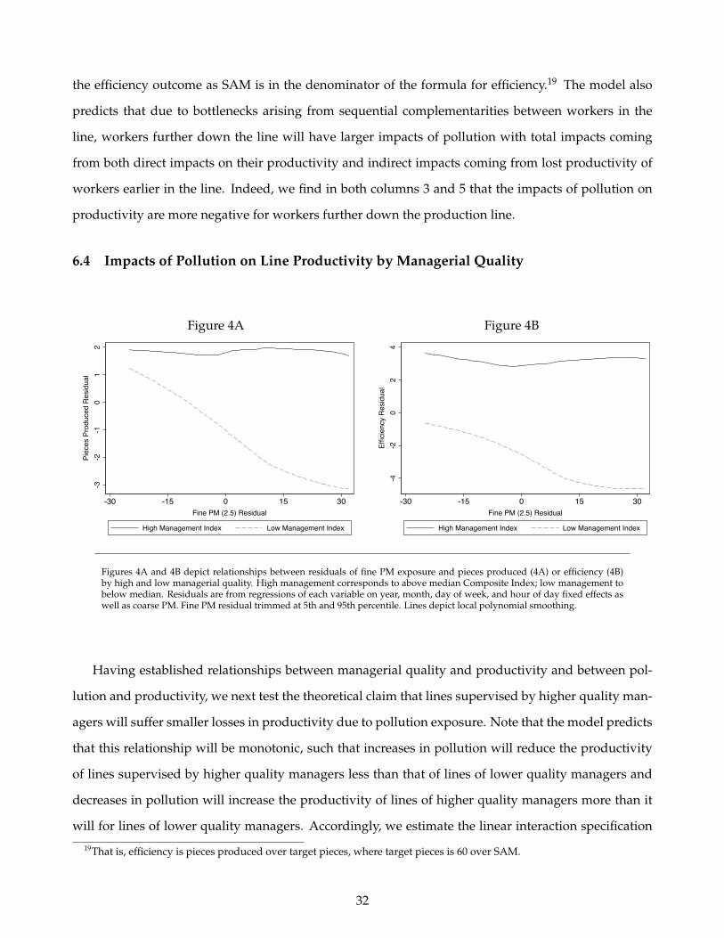
the efficiency outcome as SAM is in the denominator of the formula for efficiency.19 The model also

predicts that due to bottlenecks arising from sequential complementarities between workers in the

line, workers further down the line will have larger impacts of pollution with total impacts coming

from both direct impacts on their productivity and indirect impacts coming from lost productivity of

workers earlier in the line. Indeed, we find in both columns 3 and 5 that the impacts of pollution on

productivity are more negative for workers further down the production line.

6.4 Impacts of Pollution on Line Productivity by Managerial Quality

Figure 4A

-3-2

-10

12

Piec

es P

rodu

ced

Res

idua

l

-30 -15 0 15 30Fine PM (2.5) Residual

High Management Index Low Management Index

Figure 4B

-4-2

02

4Ef

ficie

ncy

Res

idua

l

-30 -15 0 15 30Fine PM (2.5) Residual


Figures 4A and 4B depict relationships between residuals of fine PM exposure and pieces produced (4A) or efficiency (4B)by high and low managerial quality. High management corresponds to above median Composite Index; low management tobelow median. Residuals are from regressions of each variable on year, month, day of week, and hour of day fixed effects aswell as coarse PM. Fine PM residual trimmed at 5th and 95th percentile. Lines depict local polynomial smoothing.

Having established relationships between managerial quality and productivity and between pol-

lution and productivity, we next test the theoretical claim that lines supervised by higher quality man-

agers will suffer smaller losses in productivity due to pollution exposure. Note that the model predicts

that this relationship will be monotonic, such that increases in pollution will reduce the productivity

of lines supervised by higher quality managers less than that of lines of lower quality managers and

decreases in pollution will increase the productivity of lines of higher quality managers more than it

will for lines of lower quality managers. Accordingly, we estimate the linear interaction specification

19That is, efficiency is pieces produced over target pieces, where target pieces is 60 over SAM.

32

Table 7: Pollution and Line Productivity by Managerial Quality

(1) (2) (3) (4) (5) (6)

Production Problem Solving Index X Fine PM 0.48718*** 0.52112***(0.12794) (0.13269)

Monitoring and Reallocation Index X Fine PM 1.09919*** 1.09415***(0.31340) (0.30370)

Composite Index X Fine PM 0.45384*** 0.47403***(0.10835) (0.11144)

Fine PM -2.04335*** -2.66716*** -2.65341*** -2.05369*** -2.60206*** -2.66560***(0.40296) (0.55562) (0.51522) (0.40984) (0.54156) (0.52416)

Production TargetCoarse PM and Interaction Controls

Year, Month, Day-of-Week, Hour-of-Day FE Yes Yes Yes Yes Yes YesLine FE Yes Yes Yes Yes Yes Yes

Observations 11,974 11,974 11,974 11,974 11,974 11,974Mean of Dependent Variable 50.38 48.82

Notes: Robust standard errors in parentheses (*** p<0.01, ** p<0.05, * p<0.1). Clustering is done at the date-hour level. See Table A3 for robustness to within-line correlation in errors.

Table 6Pollution and Line Productivity by Managerial Quality



LinearControl Regressor Outcome Denominator

described in equation 13. This functional form decision is validated by the graphical representation

of these interaction effects depicted in Figures 4A and 4B, which show that lines of managers with

above median Composite Index values have roughly flat productivity-pollution gradients, while lines of

managers with below median Composite Index values have starkly negative gradients for both produc-

tivity measures. The analogous regression results from the estimation of equation 13 reported in Table

7 verify these patterns. Specifically, we find that a one unit increase in one of the managerial quality

indices offsets roughly 1/5 to over 1/3 of the impact of pollution on the lowest quality managers (i.e.,

those with managerial index value of 0). When scaled by the possible range of values for each index,

we find that the highest quality managers suffer losses roughly 75 to nearly 100% smaller than do the

lowest quality managers.

6.5 Task Match Adjustment in Response to Pollution

Next, we empirically establish task reallocation as a primary mechanism by which the attenuation

in pollution impacts on productivity for higher quality managers shown in Table 7 is achieved. We

start by estimating equation 12 with task match adjustment as the outcome and more general func-

tional forms of the pollution measure as the regressors of interest. Specifically, note that the model

predicts that task reallocation responses to pollution fluctuations will not be monotonic like the im-

33

Figure 5

-.10

.1.2

.3An

y Ta

sk S

huffl

ing

Res

idua

l

-30 -15 0 15 30Fine PM (2.5) Residual

Month, Day of Week, Hour FE Added Line FEMean in Integer PM Residual Bin

Figure 5 depicts relationship between residuals of fine PM exposure and the dummy for any task shuffling. Residuals are fromregressions of each variable on year, month, day of week, and hour of day fixed effects as well as coarse PM. Fine PM residualtrimmed at 5th and 95th percentile. Scatter depicts mean residual of task shuffling within integer fine PM residual bins, Linesdepict local polynomial smoothing with and without production line fixed effects included in regression producing residuals.

pacts on productivity, but will rather be symmetric in direction at least (if not perfectly in magnitude)

around the “expected” level of pollution (or, interchangeably in the model, expected level of worker ef-

fort). That is, as pollution increases, task reallocation should increase in response to reoptimize output

(i.e., to forego full losses in output due to losses in individual worker productivity) and as pollution

decreases task reallocation should also increase to reoptimize output (i.e., to capture increases in indi-

vidual worker productivity).

Accordingly, we replace linear pollution terms with measures of two alternate forms: 1) the abso-

lute value of deviations from median pollution by production floor, day of week, hour of day, month

of year, and year), and 2) the above median deviation and absolute value of below median deviation

as separate regressors. The graphical relationship between task reallocation and pollution exposure

depicted in Figure 5 and the estimates in Table 8 show that indeed task match adjustment increases

with pollution exposure, though this seems to be mostly driven by above median pollution values.

That is, a change in pollution of one standard deviation from the time and floor-specific median pol-

34

Table 8: Pollution and Task Match Adjustment

(1) (2) (3) (4)

Absolute Value Deviations from Median Fine PM 0.02747*** 0.02572***(0.00815) (0.00777)

Above Median Fine PM Spline 0.03263*** 0.03136***(0.00877) (0.00830)

Below Median Fine PM Spline (Absolute Value) 0.00689 0.00406(0.01550) (0.01530)

Coarse PM and Interaction ControlsAbsolute Deviations from

MedianAbove and Below Distance

from Median SplinesAbsolute Deviations from

MedianAbove and Below Distance

from Median Splines

Line FE No Yes No YesYear, Month, Day-of-Week, Hour-of-Day FE Yes Yes Yes Yes

Observations 14,342 14,342 14,342 14,342Mean of Dependent Variable


Table 7Pollution and Task Match Adjustment

Any Task Match Adjustment

1(at least one worker on line reassigned to a different task this hour from last hour)

0.42

lution increases the probability of any task match adjustment on the line by 2.75 percentage points on

average with above median values contributing more than 3 percentage points to the effect. We show

next that the small impacts for below median pollution values are driven by heterogeneity in impacts

across managerial quality.

6.6 Task Match Adjustment in Response to Pollution by Managerial Quality

The graphical representation of the relationship between task reallocation and pollution exposure for

above and below median Composite Index managerial quality values depicted in Figure 6 and the analo-

gous regression estimates presented in Table 9 serve as empirical tests of the claim from the theory that

higher quality managers engage in significantly more task reallocation in response to pollution than

do lower quality measures. Specifically, the highest quality managers are more than 12.5 percentage

points more likely to engage in task match adjustment in response to pollution on average than are

the lowest quality managers (using composite index estimates); more than 20 percentage points more

likely to respond with task reallocation to below median deviations in pollution.

Next, to further support results using specific survey measures and constructed indices for manage-

rial quality presented thus far, we construct a supervisor residual TFP measure as described in section

5 and include the interaction of this measure with the pollution measures as additional terms in the

35

Table 9: Pollution and Task Match Adjustment by Managerial Quality

(1) (2) (3) (4) (5) (6)

Production Problem Solving Index X Absolute Val Dev Fine PM 0.02826***(0.00817)

Monitoring and Reallocation Index X Absolute Val Dev Fine PM 0.05883***(0.02062)

Composite Index X Absolute Val Dev Fine PM 0.02531***(0.00665)

Production Problem Solving X Above Median PM Spline 0.03064***(0.00815)

Production Problem Solving X Below Median PM Spline 0.04764***(0.01668)

Monitoring and Reallocation X Above Median PM Spline 0.05736***(0.02059)

Monitoring and Reallocation X Below Median PM Spline 0.09705**(0.03998)

Composite Index X Above Median Fine PM Spline 0.02623***(0.00655)

Composite Index X Below Median Fine PM Spline 0.04265***(0.01348)

Absolute Value Deviation from Median Fine PM -0.03353 -0.06630* -0.06721**(0.02095) (0.03423) (0.02764)

Above Median Fine PM Spline -0.03886* -0.05901* -0.06874**(0.02121) (0.03439) (0.02759)

Below Median Fine PM Spline -0.08641** -0.14019** -0.14398***(0.03892) (0.06437) (0.05223)

Coarse PM Controls and Interactions Abs Dev Splines Abs Dev Splines Abs Dev SplinesYear, Month, Day-of-Week, Hour-of-Day FE Yes Yes Yes Yes Yes Yes

Observations 11,974 11,974 11,974 11,974 11,974 11,974Mean of Dependent Variable

Notes: Robust standard errors in parentheses (*** p<0.01, ** p<0.05, * p<0.1). Clustering is done at the date-hour level. See Table A4 for robustness to within-line correlation in errors.

Table 8Pollution and Task Match Adjustment by Managerial Quality



0.42

36

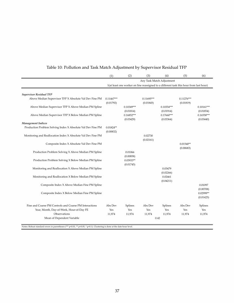
Table 10: Pollution and Task Match Adjustment by Supervisor Residual TFP

(1) (2) (3) (4) (5) (6)

Supervisor Residual TFP Above Median Supervisor TFP X Absolute Val Dev Fine PM 0.11467*** 0.11695*** 0.11276***

(0.01792) (0.01845) (0.01819)Above Median Supervisor TFP X Above Median PM Spline 0.10349*** 0.10354*** 0.10161***

(0.01814) (0.01914) (0.01854)Above Median Supervisor TFP X Below Median PM Spline 0.16852*** 0.17660*** 0.16558***

(0.03429) (0.03364) (0.03440)Management Indices

Production Problem Solving Index X Absolute Val Dev Fine PM 0.01824**

(0.00832)Monitoring and Reallocation Index X Absolute Val Dev Fine PM 0.02730

(0.02161)Composite Index X Absolute Val Dev Fine PM 0.01540**

(0.00683)Production Problem Solving X Above Median PM Spline 0.01066

(0.00858)Production Problem Solving X Below Median PM Spline 0.03933**

(0.01745)Monitoring and Reallocation X Above Median PM Spline 0.03479

(0.02266)Monitoring and Reallocation X Below Median PM Spline 0.02461

(0.04211)Composite Index X Above Median Fine PM Spline 0.01097

(0.00708)Composite Index X Below Median Fine PM Spline 0.02999**

(0.01425)

Fine and Coarse PM Controls and Coarse PM Interactions Abs Dev Splines Abs Dev Splines Abs Dev Splines


Observations 11,974 11,974 11,974 11,974 11,974 11,974Mean of Dependent Variable


Table 9Pollution and Task Match Adjustment by Supervisor Residual TFP



0.42

37

Figure 6

-.1-.0

50

.05

Any

Task

Shu

fflin

g R

esid

ual

-30 -15 0 15 30Fine PM (2.5) Residual


Figure 6 depicts relationship between residuals of fine PM exposure and dummy for any task shuffling by high and lowmanagerial quality. High management corresponds to above median Composite Index; low management to below median.Residuals are from regressions of each variable on year, month, day of week, and hour of day fixed effects as well as coarsePM. Fine PM residual trimmed at 5th and 95th percentile. Lines depict local polynomial smoothing.

otherwise identical specification reported in Table 9. These results are reported in Table 10 and show

that “better” managers as defined by the residual productivity of the lines they supervise respond to

pollution with task reallocation in much the same way as do higher quality managers as defined by our

indices. However, rather interestingly, the inclusion of this strong residual productivity quality mea-

sure does not fully absorb or obviate the impacts of our original managerial quality indices. Indeed,

the managerial index coefficients remain significant in many specifications and roughly 50 to 60% the

magnitude of those in Table 9. We interpret these results as strong evidence in support of the validity

of our managerial quality measures as well as evidence that these measures contain information not

immediately observable from productivity data alone. Next, we investigate what the additional infor-

mation in the managerial quality indices might actually be and what personality or management style

traits might predict higher managerial quality.

38

Table 11: Partial Correlations with Supervisor Residual TFP and Managerial Quality Indices

(1) (2) (3) (4) (5) (6) (7)

Production Problem Solving Index 0.00345(0.00712)

Monitoring and Reallocation Index 0.04827**(0.01691)

Composite Index 0.00802(0.00713)

Management PracticesMeeting Targets (ME) -0.04175 0.12138*** 0.00347 0.12485**

(0.03238) (0.04586) (0.03578) (0.05770)Encouraging Star Performers (ME) 0.01218 0.09348* 0.22143*** 0.31491***

(0.02475) (0.05209) (0.04064) (0.06554)Keeping Talented Workers (ME) 0.02827** 0.09931** 0.06349* 0.16280***

(0.00955) (0.04889) (0.03814) (0.06151)Management Style

Positive Leadership Behavior (ME) -0.02701 0.11269** 0.04808 0.16077***(0.01520) (0.04700) (0.03666) (0.05913)

Passive Conflict Resolution Style (ME) -0.00114 -0.08840* -0.08603** -0.17444***(0.02322) (0.04776) (0.03726) (0.06009)

PersonalityConscientiousness (ME) -0.02590 0.08690* 0.07661* 0.16351**

(0.02159) (0.05137) (0.04007) (0.06463)Locus of Control (ME) -0.00362 -0.02683 -0.04518 -0.07201

(0.01786) (0.03694) (0.02882) (0.04648)Perseverance (ME) 0.02203 0.07269 0.02086 0.09355

(0.01833) (0.04877) (0.03805) (0.06136)Self-Esteem (ME) 0.02223 -0.03549 -0.04102 -0.07651

(0.01434) (0.04746) (0.03703) (0.05972)

Observations 1,649 1,649 1,649 1,649 473 473 473SD of Dependent Variable 0.76 0.60 1.06

Mean of Dependent Variable 2.26 1.46 3.71

Table 10Partial Correlations with Supervisor Residual TFP and Managerial Quality Indices

Notes: Robust standard errors in parentheses (*** p<0.01, ** p<0.05, * p<0.1). Clustering is done at the line level.

Supervisor Residual TFP

Residual from regression of ln(pieces produced) on worker and time FE

Production Problem

Solving Index

Monitoring and

Reallocation Index

Composite Index

0.000.72

39

6.7 Managerial Quality Unpacked: Practices, Skills, and Personality

In Table 11 we report estimates of partial correlations from descriptive regressions relating the man-

agerial indices to supervisor residual TFP and to additional measures from the management survey

of management practices, management style, and personality traits. Columns 1 through 4 of Table 11

show that in fact our managerial quality indices are positively correlated with the supervisor residual

TFP measure, but this correlation is small and somewhat weak. Column 5 shows that in fact many

other survey measures for management practices, style, and personality traits are equally weakly cor-

related with supervisor residual TFP. On the other hand, we find that many of these measures are

strongly correlated with our managerial quality indices. In particular, we find that the more specific

practices the manager reports engaging in to meet targets, positively reinforce high performing work-

ers, and retain these high performing workers, the higher the managerial quality as measured by all of

our indices. Additionally, positive leadership behaviors and less passive conflict resolution correlate

positively with our indices.

Personality measures in general show weaker correlations, but we find some evidence that con-

scientiousness is positively correlated with all of our managerial indices. We interpret these results

as further evidence that our managerial quality indices have incremental information beyond what

is directly observable in average productivity alone and are important determinants of production

decisions in general as well as determinants specifically of responses to productivity shocks.

7 Conclusion

Managerial quality has been shown to be a crucial determinant of firm and worker productivity. In this

paper, we model the role of managerial quality on productivity via the re-optimization of production in

response to worker and task-specific productivity shocks. We estimate the model using data on hourly

individual productivity, managerial quality, and high frequency fluctuations in air pollution, which

negatively impacts productivity. We note the presence of intra-firm heterogeneity on two important

aspects of management – optimizing the assignment of workers to tasks and identifying and resolving

production issues - and estimate the impact of this heterogeneity on productivity.

We show that not only do higher quality managers achieve higher productivity on average, they are

able to avoid losses from negative productivity shocks caused by air pollution through re-optimization

of worker-task matching. Lines supervised by the highest quality managers suffer much smaller losses

40

as a result of air pollution productivity shocks by way of more dynamic worker reallocation.

We validate our measures of managerial quality using residual productivity measures of supervi-

sor TFP, and establish the incremental value of such measures of managerial quality above and beyond

measures of observable productivity. We also provide descriptive evidence of the specific practices,

management styles, and personality traits that contribute to managerial quality index values. These

results contribute to explaining the mechanisms through which managerial inattention impacts pro-

ductivity.

Our results hopefully also prompt further questions to be explored in future work. In particular,

whether these aspects of quality are immutable, or responsive to training is an important question,

as is the question of whether managers with similar goals respond differently to different incentive

structures. While these are outside the scope of this study, they form interesting questions for future

work.

41

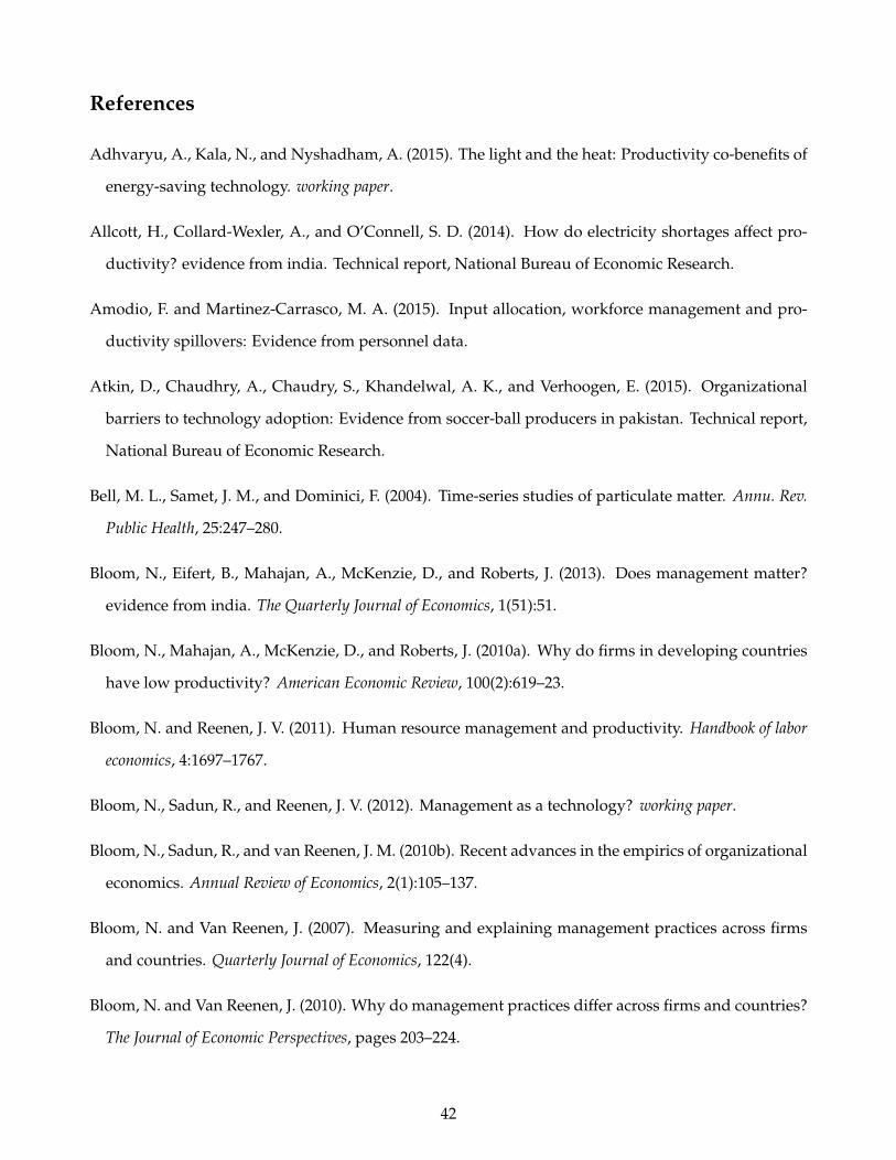
References

Adhvaryu, A., Kala, N., and Nyshadham, A. (2015). The light and the heat: Productivity co-benefits of

energy-saving technology. working paper.

Allcott, H., Collard-Wexler, A., and O’Connell, S. D. (2014). How do electricity shortages affect pro-

ductivity? evidence from india. Technical report, National Bureau of Economic Research.

Amodio, F. and Martinez-Carrasco, M. A. (2015). Input allocation, workforce management and pro-

ductivity spillovers: Evidence from personnel data.

Atkin, D., Chaudhry, A., Chaudry, S., Khandelwal, A. K., and Verhoogen, E. (2015). Organizational

barriers to technology adoption: Evidence from soccer-ball producers in pakistan. Technical report,

National Bureau of Economic Research.

Bell, M. L., Samet, J. M., and Dominici, F. (2004). Time-series studies of particulate matter. Annu. Rev.

Public Health, 25:247–280.

Bloom, N., Eifert, B., Mahajan, A., McKenzie, D., and Roberts, J. (2013). Does management matter?

evidence from india. The Quarterly Journal of Economics, 1(51):51.

Bloom, N., Mahajan, A., McKenzie, D., and Roberts, J. (2010a). Why do firms in developing countries

have low productivity? American Economic Review, 100(2):619–23.

Bloom, N. and Reenen, J. V. (2011). Human resource management and productivity. Handbook of labor

economics, 4:1697–1767.

Bloom, N., Sadun, R., and Reenen, J. V. (2012). Management as a technology? working paper.

Bloom, N., Sadun, R., and van Reenen, J. M. (2010b). Recent advances in the empirics of organizational

economics. Annual Review of Economics, 2(1):105–137.

Bloom, N. and Van Reenen, J. (2007). Measuring and explaining management practices across firms

and countries. Quarterly Journal of Economics, 122(4).

Bloom, N. and Van Reenen, J. (2010). Why do management practices differ across firms and countries?

The Journal of Economic Perspectives, pages 203–224.

42

Brook, R. D., Brook, J. R., Urch, B., Vincent, R., Rajagopalan, S., and Silverman, F. (2002). Inhalation

of fine particulate air pollution and ozone causes acute arterial vasoconstriction in healthy adults.

Circulation, 105(13):1534–1536.

Bruhn, M., Karlan, D., and Schoar, A. (2010). What capital is missing in developing countries? The

American Economic Review, pages 629–633.

Caselli, F. (2005). Accounting for cross-country income differences. Handbook of economic growth, 1:679–

741.

Chang, T., Graff Zivin, J., Gross, T., and Neidell, M. (2014). Particulate pollution and the productivity

of pear packers. NBER Working Paper, (w19944).

Dell, M., Jones, B. F., and Olken, B. A. (2012). Temperature shocks and economic growth: Evidence

from the last half century. American Economic Journal: Macroeconomics, 4(3):66–95.

Dockery, D. W. and Pope, C. A. (1994). Acute respiratory effects of particulate air pollution. Annual

review of public health, 15(1):107–132.

Ellison, S. F. and Snyder, C. M. (2014). An empirical study of pricing strategies in an online market

with high-frequency price information.

Graff Zivin, J. and Neidell, M. (2012). The impact of pollution on worker productivity. American

Economic Review, 102:3652–3673.

Hall, R. E. and Jones, C. I. (1999). Why do some countries produce so much more output per worker

than others? The Quarterly Journal of Economics, 114(1):83–116.

Hanna, R. and Oliva, P. (2016). The effect of pollution on labor supply: Evidence from a natural

experiment in mexico city. Technical report.

Heath, R. (2011). Why do firms hire using referrals? evidence from bangladeshi garment factories.

manuscript, University of Washington.

Heath, R. and Mobarak, A. M. (2015). Manufacturing growth and the lives of bangladeshi women.

Journal of Development Economics, 115:1–15.

43

Hjort, J. (2014). Ethnic divisions and production in firms. The Quarterly Journal of Economics,

129(4):1899–1946.

Lazear, E. P., Shaw, K. L., and Stanton, C. T. (2014). The value of bosses. working paper.

Macchiavello, R., Menzel, A., Rabbani, A., and Woodruff, C. (2015). Challenges of change: An experi-

ment training women to manage in the bangladeshi garment sector. Technical report.

Marx, B., Pons, V., and Suri, T. (2015). Diversity and team performance in a kenyan organization.

Mills, N. L., Tornqvist, H., Robinson, S. D., Gonzalez, M., Darnley, K., MacNee, W., Boon, N. A.,

Donaldson, K., Blomberg, A., Sandstrom, T., et al. (2005). Diesel exhaust inhalation causes vascular

dysfunction and impaired endogenous fibrinolysis. Circulation, 112(25):3930–3936.

Pope, C., Dockery, D., et al. (1999). Epidemiology of particle effects. Air pollution and health, 31:673–705.

Pope, C. A. and Dockery, D. W. (2006). Health effects of fine particulate air pollution: lines that connect.

Journal of the Air & Waste Management Association, 56(6):709–742.

Reis, R. (2006). Inattentive producers. The Review of Economic Studies, 73(3):793–821.

Schoar, A. (2014). The importance of being nice: Supervisory skill training in the cambodian garment

industry. working paper.

Souza, M. B., Saldiva, P. H., Pope, C. A., and Capelozzi, V. L. (1998). Respiratory changes due to long-

term exposure to urban levels of air pollution a histopathologic study in humans. CHEST Journal,

113(5):1312–1318.

Staritz, C. (2010). Making the Cut?: Low-income Countries and the Global Clothing Value Chain in a Post-

quota and Post-crisis World. World Bank Publications.

Stolarick, K. M. et al. (1999). Are Some Firms Better at It?: Differing Relationships Between Productivity and

IT Spending. Center for Economic Studies, US Department of Commerce, Bureau of the Census.

Sudarshan, A. and Tewari, M. (2013). The economic impacts of temperature on industrial productivity:

Evidence from indian manufacturing.

Syverson, C. (2011). What determines productivity? Journal of Economic Literature, 49(2):326–365.

44

Tybout, J. R. (2000). Manufacturing firms in developing countries: How well do they do, and why?

Journal of Economic literature, pages 11–44.

Wilson, W. E. and Suh, H. H. (1997). Fine particles and coarse particles: concentration relationships

relevant to epidemiologic studies. Journal of the Air & Waste Management Association, 47(12):1238–

1249.

World Bank, D. P. G. (2012). World Development Indicators 2012. World Bank Publications.

45

A Checks and Robustness

In Figure A1, we plot fine and coarse PM levels across days of the week, including Sundays on which

very little production occurs at the garment factory. We see that indeed fine PM continue to remain at

roughly the same levels as those during the work week; while coarse PM drops measurably on Sun-

days, indicating that coarse PM is more likely produced through factory activity than fine PM. Figure

A2 plots fine and coarse PM levels across hours of the day including non-production hours. Coarse

PM shows high levels during production hours with a dip in levels before and after production hours

as well as during lunch hours. Fine PM shows peaks during commuting hours and lower levels dur-

ing peak production. These patterns suggest that coarse PM is more likely produced through garment

manufacturing activity, while fine PM appears more likely to be produced through automobile exhaust

during high traffic hours.

Figure A1: Daily PM

010

020

030

040

050

0C

oars

e PM

025

5075

100

Fine

PM

Sunday Monday Tuesday Wednesday Thursday Friday Saturday

Day of the Week

Fine PM Coarse PM

Figure A2: Hourly PM

020

040

060

080

0C

oars

e PM

025

5075

100

Fine

PM

12AM 2AM 4AM 6AM 8AM 10AM 12PM 2PM 4PM 6PM 8PM 10PM

Hour of the Day

Fine PM Coarse PM

Figures A1 and A2 depict mean of fine and coarse PM levels across days of the week (A1) and hours of the day (A2). Verticalline denotes start of production week in Figure A1. In Figure A2, vertical solid lines denote start and end of production day;dashed lines denote lunch hour; and dotted lines commuting hours.

In Table A1, we show expanded summary statistics for the managerial quality indices.

In Table A2, we show robustness of estimates from Table 5 to the inclusion of additional controls

for weather. We find that the results are nearly unaffected by these additional controls.

In Table A3, we show robustness of estimates from Table 7 to various estimators that allow for

differing types of within-line correlation in errors. The random effect estimator allows for errors to be

46

Table A1: Managerial Quality Indices Summary Statistics

Frequency Percent CummulativeProduction Problem Solving Index

0 1,144 9.55 9.551 1,161 9.7 19.25

1.5 2,113 17.65 36.92 195 1.63 38.53

2.333333 838 7 45.522.5 2,229 18.62 64.14

2.666667 1,110 9.27 73.413 3,184 26.59 100

Monitoring and Reallocation Index0.5 174 1.45 1.451 2,306 19.26 20.71

1.333333 1,110 9.27 29.981.5 3,189 26.63 56.61

1.666667 838 7 63.612 4,357 36.39 100

Composite Index1 1144 9.55 9.55

2.5 1335 11.15 20.73 970 8.10 28.8

3.5 2305 19.25 48.054 1948 16.27 64.32

4.5 2167 18.10 82.425 2105 17.58 100

Production Problem Solving Monitoring and Shuffling CompositePairwise Correlation Production Problem Solving Index 1 Monitoring and Reallocation Index 0.3999 1 Composite Index 0.9502 0.6657 1

Table A1Managerial Quality Indices Summary Statistics

47

Table A2: Pollution and Productivity by Managerial Quality (Robustness to Weather Controls)

(1) (2) (3)

Random Effects (Equicorrelated Within Line)Production Problem Solving Index X Abs Val Dev Fine PM 0.00108***

(0.00034)Monitoring and Reallocation Index X Abs Val Dev Fine PM 0.00225***

(0.00085)Composite Index X Fine PM 0.00097***

(0.00028)GLS (Line-specific AR(1))

Production Problem Solving Index X Abs Val Dev Fine PM 0.00084***(0.00032)

Monitoring and Reallocation Index X Abs Val Dev Fine PM 0.00114(0.00080)

Composite Index X Abs Val Dev Fine PM 0.00070***(0.00027)

Fine and Coarse PM ControlsYear, Month, Day-of-Week, Hour-of-Day FE Yes Yes Yes

Observations 11,974 11,974 11,974Mean of Dependent Variable

Above and Below Median Absolute Value Deviation Splines

0.42

Notes: Robust standard errors in parentheses (*** p<0.01, ** p<0.05, * p<0.1). Errors estimated according to models described in each panel above.

Table A4Pollution and Task Match Adjustment by Managerial Quality (Robust to Within-Line Correlation)

Any Task Match Adjustment1(at least one worker on line reassigned to a different task this hour from last

hour)

correlated within line over time, but assumes this correlation is fixed. This assumption is likely true

conditional on the full set of time fixed effects included in all specifications. The GLS model reported

allows for a line-specific AR(1) process in the errors, relaxing the assumption in the random effects

model. The GLS model is however less efficient under the random effects assumptions. We find that

the overall pattern of results as well as statistical significance is generally preserved.

In Table A4, we show robustness of estimates from Table 9 to the same estimators from Table A3

that allow for differing types of within-line correlation in errors. Once again, we find that the overall

pattern of results as well as statistical significance is generally preserved.

48

Table A3: Managerial Quality and Line Productivity (Robustness to Within-Line Correlation)

(1) (2) (3) (4) (5) (6) (7) (8)

Fine PM (Std) -0.59952*** -0.68705*** -0.58913*** -1.57081*** -0.54561*** -0.65591*** -0.54455*** -1.43305***(0.14326) (0.17938) (0.21790) (0.26647) (0.14467) (0.16847) (0.20907) (0.23903)

Additional Weather Controls Date FEMean Daily

TempDaily Temp &

RainHourly Temp and Rel Hum

Date FEMean Daily

TempDaily Temp &

RainHourly Temp and Rel Hum

Coarse PM ControlsYear, Month, Day-of-Week, Hour-of-Day FE Yes Yes Yes Yes Yes Yes Yes Yes

Line FE No Yes Yes Yes No Yes Yes YesObservations 1,054,962 1,054,962 493,521 392,009 1,054,962 1,054,962 493,521 392,009

Notes: Robust standard errors in parentheses (*** p<0.01, ** p<0.05, * p<0.1). Clustering is done at the worker level.

Table A2Robustness to Weather Controls

Pieces Produced

pieces produced by worker this hour

Efficiency

(pieces produced / target pieces)

Linear

Table A4: Pollution and Task Match Adjustment by Managerial Quality (Robustness to Within-LineCorrelation)

(1) (2) (3) (4) (5) (6)

Random Effects (Equicorrelated Within Line)Production Problem Solving Index X Fine PM 0.01865*** 0.01995***

(0.00514) (0.00504)

Monitoring and Reallocation Index X Fine PM 0.04208*** 0.04189***

(0.01196) (0.01171)

Composite Index X Fine PM 0.01738*** 0.01815***

(0.00422) (0.00414)

GLS (Line-specific AR(1))Production Problem Solving Index X Fine PM 0.00962** 0.00896**

(0.00412) (0.00404)

Monitoring and Reallocation Index X Fine PM 0.00265 0.00920

(0.00940) (0.00924)

Composite Index X Fine PM 0.00675** 0.00710**

(0.00340) (0.00334)

Fine and Coarse PM Controls


Observations 11,974 11,974 11,974 11,974 11,974 11,974

Mean of Dependent Variable

Linear

50.38 48.82

Notes: Robust standard errors in parentheses (*** p<0.01, ** p<0.05, * p<0.1). Errors estimated according to models described in each panel above.

Table A3

Pollution and Line Productivity by Managerial Quality (Robust to Within-Line Correlation)



49

B Data Appendix

B.1 Productivity and other Production Variables

• Pieces Produced: Number of garments produced at the hourly level (per worker or per line de-

pending on the regression specification). Line-level number of garments in a given hour is the

average of the number of garments produced at the worker-level.

• Standard Allowable Minutes (SAM): This is a measure of how many minutes a particular garment

style should be completed in. For instance, a garment style with a SAM of .5 is deemed to take

a half minute to produce one complete garment. It is a standardized measure across the global

garment industry and is drawn from an industrial engineering database, although it might be

amended to account for stylistic variations from the representative garment style in the database.

• Target Quantity: The target quantity for a given unit of time for a line producing a particular style

is calculated as the unit of time in minutes divided by the SAM. That is, the target quantity to be

produced by a line in an hour for a style with a SAM of .5 will be60

0.5= 120 garments per hour.

• Efficiency:(

Number of garments producedNumber of target garments

)*100 at the hourly level (per worker or per line de-

pending on the regression specification). Line-level number efficiency in a given hour is the mean

of worker-level efficiency in that hour.

B.2 Worker Task Adjustment

• Any Task Match Adjustment: 1[any worker was reassigned on the line to a different task than they

were doing the previous hour].

B.3 Worker Position in the Line

• Seat in Line: This indicates the relative placement of the worker in the line in order of the flow of

production. e.g. the worker conducting the first operation in the production process is said to be

in seat 1, the worker next to him who takes worker 1’s production and adds to it in seat 2, and so

on.

50

B.4 Pollution

• Fine PM(Std): Fine (0.5-2.5 microns in diameter) particulate matter (PM) concentration (µg/m3)/SD(fine

PM concentration)

• Coarse PM(Std): Coarse (2.5-10 microns in diameter) particulate matter (PM) concentration (µg/m3)/SD(coarse

PM concentration)

B.5 Management

B.5.1 Managerial Quality

• Production Problem Solving Index (0-3): It is the sum of the following three indicator variables,

and ranges from 0 to 3 (if the line is supervised by more than one supervisor, the indicators are

averaged across supervisors before summing to construct the index).

– 1[supervisor generally learns about production issues from talking to workers].

– 1[ supervisor is fluent in the native language of the majority of the workers]

– 1[whether the supervisor generally solves production issues on their own]

• Monitoring and Reallocation Index (0-2): It is the sum of the following two indicator variables, and

so ranges from 0 to 2.

– 1[reported making rounds of the line to monitor production at least every 10 min]. If the

line is supervised by more than one supervisor, the minimum value is taken to maximize

the variation in this variable.

– 1[reported that they would try to replace a worker that was performing poorly]. If the line

is supervised by more than one supervisor, the indicators are averaged across supervisors

before summing to construct the index.

• Composite Index (0-5): The sum of the Production Problem Solving Index and the Monitoring and

Reallocation Index. It is the sum of the five indicator variables comprising these indices, and so

ranges from 0 to 5.

51

B.5.2 Other Management Variables

• Supervisor TFP Residual: This is constructing by regressing log(pieces produced) 20 at the worker-

level on all time fixed effects (Year, Month, Day-of-Week, Hour-of-Day FE) and worker fixed

effects, and constructing average line level predicted residuals.

• Meeting Targets (ME): This measure captures the effort exerted by supervisors in meeting targets.

Supervisors were asked what practices they follow to ensure production targets are met. Each

practice was coded as an indicator variable and comprised of the following indicators:

– 1[Do rounds of the line to ensure things are in order]

– 1[Talk to workers individually]

– 1[Provide positive reinforcement to high-performing workers]

– 1[Make low-performing workers aware of their work]

– 1[Demonstrate how to work by example]

The final measure was computed as the mean effect normalization of these five indicator vari-

ables.21

• Encouraging Star Performers (ME): This measure captures the effort exerted by supervisors in en-

couraging and retaining high performing workers on their line. Supervisors were asked what

practices they follow to encourage a worker who was very productive and fulfilled their tar-

gets in a timely manner. Each practice was coded as an indicator variable and comprised of the

following indicators:

– 1[Commend the worker on their work/effort]

– 1[Praise the worker in presence of other workers]

– 1[Put in good word for workers to upper-level management]

– 1[Recommend the worker for a promotion]

– 1[Other]20to correspond to the log-linearized Cobb-Douglas production function21The mean effect normalization is calculated by subtracting the mean and dividing the standard deviation for each indi-

cator variable, adding up these normalized variables, and then subtracting the mean and dividing the standard deviationfor this composite variable. While this maximizes the variation in the variable, using the simple sum of the binary variablesdoes not significantly alter the results using this variable.

52

The final measure was computed as the mean effect normalization of the above indicator vari-

ables.

• Keeping Talented Workers (ME): This measure captures the effort exerted by supervisors in retain-

ing high performing workers on their line. Supervisors were asked what practices they follow to

retain a very productive worker who wanted to leave the company . Each practice was coded as

an indicator variable and comprised of the following indicators:

– 1[Talk to the worker directly to convince them to stay]

– 1[Put in good word for the worker to upper-level management]

– 1[Recommend a salary increase for the worker]

– 1[Recommend the worker for a promotion]

– 1[Other]

The final measure was computed as the mean effect normalization of the above variables.

• Positive Leadership Behavior(ME): This measure captures the net number of behaviors supervisors

identify engaging in that can be described as positive management behaviors. Supervisors were

asked about the extent (measured on a 5-point scale of agreement ranging from Strongly Agree

to Strongly Disagree) to which they engaged in 18 positive and 6 negative behaviors. The score

from each variable was added up for positive and negative behaviors and the score from the

negative behaviors was then subtracted from the score for positive behaviors.

The positive practices were the following:

– I do personal favors for workers in my line

– I make my attitudes clear to the workers in my line

– I do little things to make it pleasant to be a member of my line

– I try out new ideas with my line

– I act as the real leader of the line

– I am easy to understand

– I find time to listen to members of the line

– I give advance notice of changes

53

– I look out for the personal welfare of individual workers on my line

– I assign workers on the line to particular tasks clearly

– I am the spokesman of the line

– I schedule the work to be done

– I maintain definite standards of performance

– I keep the line informed

– I back up the workers in my line in their actions

– I emphasize the meeting of deadlines

– I treat all workers in my line as my equals

– I encourage the use of uniform procedures

The negative practices were the following:

– I rule with an iron fist

– I criticize poor work

– I speak in a manner not to be questioned

– I keep to myself

– I refuse to explain my actions

– I act without consulting the line


• Passive Conflict Resolution Style (ME): This measure captures the style followed by supervisors

in resolving conflicts arising during the management process. Supervisors were asked about

the frequency (measured on a 5-point scale of frequency ranging from Very Frequently to Very

Infrequently)with which they had engaged in the following conflict resolution behaviors:

– Management problems with employees

– Had direct reports (workers who reported to that supervisor) that resisted their initiatives

– Had interpersonal conflicts between them and at least one of their direct reports

54

– Had employees who were used to doing things they way they had been done and were

reluctant to change

– Had key members of your staff that were incompetent, unmotivated, technically obsolete,

or otherwise poor performers

– Had key direct reports that lacked the experience to do their jobs without close supervision


• Contentiousness (ME): This measure captures the net number of behaviors supervisors identify

with that are predictive of contentiousness. Supervisors were asked about the extent (measured

on a 5-point scale of agreement ranging from Strongly Agree to Strongly Disagree) to which they

engaged in 5 positive and 5 negative behaviors. The score from each variable was added up for

positive and negative behaviors and the score from the negative behaviors was then subtracted

from the score for positive behaviors.

The positive behaviors were the following:

– I am always prepared

– I pay attention to details

– I get chores done right away

– I carry out my plans

– I make plans and stick to them

The negative behaviors were the following:

– I procrastinate and waste my time

– I find it difficult to get down to work

– I do just enough work to get by

– I don’t see things through

– I shirk my duties


55

• Locus of Control (ME): This measure captures the net number of beliefs supervisors identify with

that are predictive of locus of control. Supervisors were asked about the extent (measured on

a 5-point scale of agreement ranging from Strongly Agree to Strongly Disagree) to which they

believed 5 statements, one of which is positively related to locus of control and four which are

negatively related. The score from each variable was added up for the negative statements and

the score from the negative statements was then subtracted from the score for positive statement.

The positive statement was the following:

– I believe that my success depends on ability rather than luck

The negative statements were the following:

– I believe that unfortunate events occur because of bad luck

– I believe that the world is controlled by a few powerful people

– I believe some people are born lucky

– I believe in the power of fate


• Perseverance (ME): This measure captures the net number of behaviors supervisors engage in that

are predictive of perseverance. Supervisors were asked about the extent (measured on a 5-point

scale of agreement ranging from Strongly Agree to Strongly Disagree) to which they engaged in

8 behaviors, five of which is positively related to perseverance and three which are negatively

related. The score from each variable was added up for the negative statements and the score

from the negative behaviors was then subtracted from the score for positive behaviors.

The positive behaviors were the following:

– I don’t quit a task before it is finished

– I am a goal-oriented person

– I finish things despite obstacles in the way

– I am a hard worker

– I don’t get sidetracked when I work

The negative behaviors were the following:

56

– I don’t finish what I start

– I give up easily

– I do not tend to stick with what I decide to do


• Self-Esteem (ME): This measure captures the net number of beliefs supervisors identify with that

are predictive of self-esteem. Supervisors were asked about the extent (measured on a 5-point

scale of agreement ranging from Strongly Agree to Strongly Disagree) to which they believed

10 statements, five of which is positively related to self-esteem and four which are negatively

related. The score from each variable was added up for the negative statements and the score

from the negative statements was then subtracted from the score for positive statements.

The positive statements were the following:

– On the whole, I am satisfied with myself

– I feel that I have a number of good qualities

– I am able to do things as well as most other people

– I feel that I am person of worth, at least on an equal plane with others

– I take a positive attitude toward myself

The negative statements were the following:

– I feel I do not have much to be proud of

– At times, I think I am no good at all

– I certainly feel useless at times

– I wish I could have more respect for myself

– All in all, I am inclined to feel that I am a failure


57

management and shocks to worker productivity · management and shocks to worker productivity ......

Documents