worker productivity during lockdown and working from home
TRANSCRIPT
8
No. 2020-12
October 2020
Worker Productivity during Lockdown and Working from Home: Evidence from Self-
Reports
Ben Etheridge Yikai Wang University of Essex
Li Tang University of Birmingham
ISE
R W
ork
ing P
aper S
erie
s
ww
w.is
er.e
sse
x.a
c.u
k
Non-Technical Summary
The Covid-19 pandemic has caused widespread disruption to working practices. The most
noticeable change has been the vast increase in working from home. While some changes to
work are probably temporary, many could well be persistent. Even after the pandemic ends,
home working in particular is expected to be much more prevalent than previously. A key
policy issue, therefore, both in the near and the far term, is how these changes in working
practices impact productivity.
In this paper we use the Covid-19 module from the UK Household Longitudinal Survey,
which provides representative data on home workers' self-reported productivity towards the
end of the lockdown period in the UK. In this survey, anyone working from home at least
some of the time was asked about changes in their productivity since just before the
pandemic period. These data allow us to examine how productivity varies across job and
worker types and is influenced, for example, by the home environment.
Overall we find that workers at home report being approximately as productive as before the
pandemic, on average. However, productivity varies substantially across socioeconomic
groups, industries and occupations. Workers in sectors that are less suitable for home
working, according to external metrics, report productivity declines. Groups reporting worse
productivity are low earners, the self-employed and women, particularly those with children.
Finally, we document that productivity declines are associated with substantially worse
mental well-being. Using information on stated reasons for difficulty working, we provide
evidence for a causal pathway from productivity to well-being.
This paper contributes to the growing evidence on the efficacy of home work. It indicates that
home working can be effective, as long as workers have the right support. The evidence in
this paper can also contribute to the design of sector-specific policies that might be used in
the short term, such as rationed access to work places.
Worker Productivity during Lockdown and Working fromHome: Evidence from Self-Reports∗
Ben Etheridge†, Li Tang‡and Yikai Wang§
5 October, 2020
Abstract
We examine self-reported productivity of home workers during lockdown using survey data
from the UK. On average, workers report being as productive as at the beginning of the year, before
the pandemic. However, this average masks substantial differences across sectors, by working-
from-home intensities, and by worker characteristics. Workers in industries and occupations charac-
terized as being suitable for home work according to objective measures report higher productivity
on average. Workers who have increased their intensity of working from home substantially report
productivity increases, while those who previously always worked from home report productivity
declines. Notable groups suffering the worst average declines in productivity include women and
those in low-paying jobs. Declines in productivity are strongly associated with declines in mental
well-being. Using stated reasons for productivity declines, we provide evidence of a causal effect
from productivity to well-being.
Keywords: Worker Productivity, Working From Home, COVID-19, Sectors, Inequality, Gen-
der, Mental Well-Being
JEL classifications: D24, I14, I30, J22, J24
∗This paper draws on data from Understanding Society, distributed by the UK Data Service. Understanding Society isan initiative funded by the Economic and Social Research Council and various Government Departments, with scientificleadership by the Institute for Social and Economic Research, University of Essex, and survey delivery by NatCen SocialResearch and Kantar Public. Preliminary working paper version; comments welcome. All errors remain the responsibilityof the authors.†University of Essex, Department of Economics. E-mail: [email protected].‡University of Birmingham, Department of Economics. E-mail: [email protected].§University of Essex, Department of Economics. E-mail: [email protected].
1 Introduction
The Covid-19 pandemic has caused widespread disruption to working practices. The most noticeablechange has been the vast increase in working from home. The share of the labour force workingfrom home increased from around 5% to over 40% in the U.S. during the lockdown (Bloom, 2020).While some changes to working practices are probably temporary, many could very likely be persistent.Even after the pandemic ends, home working in particular is expected to be much more prevalent thanpreviously.1
A key policy issue, therefore, both in the near and the far term, is how these changes in labourpractices impact worker productivity. Despite previous research on the effects of working from home(Bloom et al., 2015), given the size of the changes seen during the pandemic the evidence base isinevitably thin. Most research since the onset of the pandemic has focused on characteristics of jobsthrough objective measures such as those provided by O*NET.2 There is little direct evidence on pro-ductivity in the new working environment and how it varies not only across job types, but also workercharacteristics.
In this paper we use the Covid-19 module from the UK Household Longitudinal Survey (UKHLS),which provides representative data on home workers’ self-reported productivity towards the end of thelockdown period in the UK, in June 2020.3 In this survey, anyone working from home (WFH) at leastsome of the time was asked about changes in their productivity since before the pandemic period, atthe beginning of the year. These data allow us to examine how productivity changes vary across joband worker types and are influenced by, for example, the presence of children. The advantage of usingindividual-level reported productivity over data obtained from, say, characteristics of jobs, is that weobtain a more direct measure of the key object of interest. The advantage of using individual-levelover aggregate data reported in national statistics is that we can examine the rich causes of productivitychanges at the micro level, as well as examining effects on other outcomes of interest. Overall we findthat workers report being approximately as productive as before the pandemic, on average. However,productivity varies substantially across socioeconomic groups, industries and occupations.
In more detail, we find that workers in industries and occupations that are less suitable for workingfrom home report lower productivities than before the pandemic. Consistently with this, and with theliterature, females and low earners also report lower productivity at home on average. The opposite
1Again, see Bloom (2020). For a wider discussion see also the dedicated discussion of the literature below.2See, for example, Dingel and Neiman (2020) and Mongey, Pilossoph, and Weinberg (2020).3In the UK, the official ‘lockdown’ began on March 23 when a widespread stay-at-home order was introduced. The
lockdown eased as the incidence of Covid declined, over May and June. On June 1, restrictions were lifted which allowedpeople to meet with up to six others from separate households in outdoor places. An accepted date for the end of lockdownis July 4, when many businesses, especially in retail and food were allowed to re-open.
1
types of workers, e.g., those in the “right” occupations and with high incomes, report higher produc-tivities than previously. More specifically, we incorporate external measures of feasibility of homework from Adams-Prassl et al. (2020b), and need for physical proximity to others from Mongey et al.(2020). The sector-level correlations between our reported productivity changes and these job-basedmeasures are always of the expected sign. In fact they are higher when comparing occupations thanindustries: For example, the correlation with feasibility of home work across occupations is 0.56, andacross industries it is 0.23. This difference suggests that while occupational job characteristics pro-vide quite accurate information about the impact of working from home on productivity, the industrycharacteristics are more noisy; it is at the job-task level that most impacts of the pandemic have beenfelt. Our direct measure of productivity changes allow us to understand how well those measures —feasibility of home working and physical proximity — capture the realized productivity changes indifferent contexts.
In addition, workers’ productivity changes correlate with other aggregate outcomes: occupationaljob losses recorded in early lockdown, and aggregate labor productivity changes at the industry level.
We then examine individual characteristics in further detail. Females, low earners and the self-employed report worse productivity outcomes than their counterparts. Their low productivity is notonly related to their job characteristics, but is also directly affected by their socioeconomic condi-tions. For example, while females are more likely to work in occupations less suitable for home work(Adams-Prassl et al., 2020b), productivity of females is also more negatively affected by the presenceof children. This finding shows the strength of the measure used here over those based purely oncharacteristics of the job.
Third, we find that home workers’ productivity during the lockdown is related to the intensity ofworking from home and its change since the prior period. Those who previously worked from home atleast sometimes and then increased the intensity of home-working experienced a productivity increase.Those who did not increase their home-working frequency or never worked from home before thepandemic report a large productivity decline. This pattern is partly explained by the occupational char-acteristics of the jobs in each category. However it also suggests two counterveiling forces: a positiveproductivity effect of increased home working alongside a direct negative effect of the pandemic itself.The productivity decline reported by those who have always worked from home is evidence of thislatter phenomenon.
A noteworthy feature of the pandemic period has been a decline in mental well-being, observedparticularly in the UK (Banks and Xu, 2020; Etheridge and Spantig, 2020). We therefore assess the as-sociation of workers’ mental well-being with productivity changes. We find strong correlations betweenthe two: those who state they get much less done at home report declines in well-being comparable
2
to the effect of an unemployment shock. We also find evidence of a causal effect from productivity towell-being: using ineffective equipment as an instrument for productivity declines, we find a 1 standarddeviation lower productivity causes a 0.24 standard deviation lower mental well-being, as measured bygeneral health questionnaire scores. This result is consistent with Etheridge and Spantig (2020) whofind that females and low income groups have experienced large deteriorations in mental well-beingcompared to their counterparts. Our paper therefore offers a novel explanation for the recent declinesin mental well-being among certain groups. It also suggests that policies that target workers in thevulnerable socioeconomic groups or certain jobs with large productivity drops may not only boostproductivity but also mental well-being on aggregate.
Related Literature
Our paper is related to four strands of literature: (1) working from home as an alternative practice; (2)sector-specific productivity changes and optimal policies during the current pandemic; (3) inequalityacross gender and socioeconomic groups, especially during difficult times such the current pandemicand other recessions; and (4) mental well-being during the current pandemic.
First, working from home and its impact on productivity have been getting increasing attention inrecent years, and especially since the Covid-19 outbreak. Bloom et al. (2015) study workers’ produc-tivity and attitude towards working from home using a random experiment on call-center workers ina Chinese travel agency. They find that home-working led to a 13% performance increase and that,after the experiment, over half of the workers chose to switch to home-working. While Bloom et al.(2015) focus on one particular narrow occupation, the Covid-19 outbreak and the lockdowns in manycountries has dramatically increased the prevalence of working from home in almost all occupations.
Felstead and Reuschke (2020) document that in the UK, while 5% of workers worked from thehome before the pandemic, the share increased to 45% in April 2020, remaining high thereafter. Theyalso find little effect of workers’ productivity at home on average during the pandemic. The samepatterns — increasing home-working and not much change in workers’ average productivity at home— are also found in Europe and North America (see Rubin et al. (2020) for Netherlands, Eurofound(2020) for the Europe as a whole, and Brynjolfsson et al. (2020) for the US).
The second strand of the literature is the sector-specific productivity of working from home, andoptimal sectoral policies. The existing papers pioneered by Dingel and Neiman (2020) use character-istics of jobs to provide predictions on home-working productivities across occupations and industries.Dingel and Neiman do this by constructing a measure of feasibility to work from home across indus-tries and occupations using data from O*NET. Adams-Prassl et al. (2020b) follow this by eliciting
3
a conceptually similar measure derived using individual self-reports. Again similarly, Mongey et al.(2020) also use O*NET to construct a measure of need for physical proximity to co-workers to carryout one’s work effectively. The direct evidence of productivity changes provided in the current papercan be used to understand how well the measures constructed from job characteristics capture the realproductivity changes across sectors, and can potentially be used in macro models of the pandemic withsector-specific shocks and optimal policies.
In this way, estimates of productivity changes by sector are important for macroeconomic modelsthat try to capture the sectoral and aggregate labor and output changes during the Covid-19 pandemic,e.g., Baqaee and Farhi (2020). Bonadio et al. (2020) study the impact of the Covid-19 pandemicon GDP growth and the role of the global supply chains. They discipline the labor supply shockacross sectors using the fraction of work that can be done from home across generations measuredby Dingel and Neiman. While the correlation of this measure with our measure of realized laborproductivity is reasonably high, there is space for improvement by obtaining better measures of realizedlabor productivity changes.
Third, the differential impacts of working from home across sectors and socioeconomic groupsimplies that inequality is strongly affected by enforced home working in the pandemic. Income in-equality has also been increasing since the 1980s both in the U.S. (Heathcote et al., 2010), and in theUK (Blundell and Etheridge, 2010). Inequality has often been found to increase during recessions (seePerri and Steinberg, 2012 for a discussion of the great recession after 2008). In the current pandemic,it is also the economically disadvantaged groups, such as low-income groups and females, that aresuffering larger declines in economic outcomes.
In this vein Alon et al. (2020) study the potentially different impacts of Covid-19 pandemic onthe employment of men and women given the gender differences in occupation and childcare. Theypredicted that women’s employment would suffer disproportionately. Adams-Prassl et al. (2020a) doc-ument that female workers report a lower ability to work from home, and Adams-Prassl et al. (2020a)document that women are more likely to lose their jobs in the UK and in the US (though not in Germany,around early April 2020). They also find worse outcomes for lower earners. Our paper contributes tothis strand of the literature by studying inequality of worker productivity across gender and socioeco-nomic groups. Our findings confirm the prediction of this literature: Females and low income groupshave suffered larger productivity declines while working from home during the lockdown, indicatingan increase in inequality.
The fourth strand of related literature is that on mental well-being during Covid-19. Early in thepandemic, international organizations and researchers warned about the resulting psychological effects(Holmes et al., 2020; World Health Organization, 2020). The pandemic imposes large risks and po-
4
tential damages to mental well-being through a variety of channels. Anxiety is caused by the disease’sspread: Fetzer et al. (2020) conduct a survey covering 58 countries and show, by exploiting time vari-ation in country-level lockdown announcements, that people’s perception of the spread of the diseasecauses lower mental well-being. Lower mental well-being is also caused by adverse economic shocks(see Chang et al., 2013; Dagher et al., 2015 for the 2008 recession, and Janke et al. (2020) for UK during2002–2016). Finally, loneliness and social isolation can be induced by quarantine (Brooks et al., 2020)and lockdown (Brodeur et al., 2020; Knipe et al., 2020; Tubadji et al., 2020).
Banks and Xu (2020) and Etheridge and Spantig (2020) document decline in mental well-beingduring the Covid-19 pandemic in the UK using the same dataset as the current paper. We add tothese papers by documenting an association between mental well-being and worker productivity. Morewidely the literature on the relation between economic conditions and mental well-being is vast; seefor example, Janke et al. (2020) who study how macroeconomic conditions affect health condition,especially mental health conditions, using British data over the period 2002–2016.
2 Data
We use the Covid-19 module from the UK Household Longitudinal Survey (UKHLS), administeredmonthly from April 2020. The analysis makes specific use of the Covid module’s third wave, conductedin June, which includes questions on self-reported productivity. These interviews were conducted in theseven days from Thursday June 25, with around 75% of interviews completed within the first three days.We merge these data with the April and May waves of the Covid module as well as with wave 9 of the‘parent’ UKHLS (also known as ‘Understanding Society’), a large-scale national survey administeredyearly from 2009. Wave 9 of the parent survey was itself administered between 2017 and 2019.
The UKHLS Covid module is conducted as a web survey. The underlying sampling frame consistsof all those who participated in the UKHLS main survey’s last two waves. To conduct the fieldwork,the sample was initially contacted using a combination of email, telephone, postal and SMS requests.Of those eligible, and who responded to the main survey wave 9, the response rate was a little under50%. To adjust our analysis for non-response, we use the survey weights provided. In addition, toallow for the fact that many respondents are related either through primary residence or through theextended family, we cluster all regressions at the primary sampling unit level. For a further discussionof the Covid module and underlying UKHLS design see (Institute for Social and Economic Research,2020).
The main variable of interest is self-reported productivity while working from home and comparedto a stated baseline. To elicit this the survey includes a bespoke question. Precisely, respondents are
5
asked as follows:“Please think about how much work you get done per hour these days. How does that compare to
how much you would have got done per hour back in January/February 2020?”If the respondent did not work from home before the pandemic, then the question ends with:“...when, according to what you have previously told us, you were not working from home?”Interviewees are then asked to respond on a Likert-type scale of 1 to 5 ranging from “I get much
more done” to “I get much less done”.We transform the variable as follows: we invert so that responses are increasing in productivity; we
re-centre so that the response “I get about the same done” is valued 0, and we divide the distributionby its standard deviation. In this way the mean response across the population can be interpreted interms of standard deviations away from a neutral effect. When discussing results we sometimes termthe resulting variable as a ‘semi-standardized’ productivity change.
It is worth discussing the question and resulting data in more detail. Notice first that the questionexplicitly attempts to ask about productivity per hour, and so corresponds to a concept of labour pro-ductivity. We examine the relationship between the variable here and aggregate productivity data fromthe National Accounts in more detail in section 3. Notice further that the question actually makes noreference to working from home itself, except in the qualifier referencing prior working location. Inprinciple, therefore, this question could be asked of workers in any location. It was in fact only askedof those working from home to save valuable survey time. In future waves it is hoped this question isasked of all respondents. Most importantly, perhaps, it should be remembered that the scale is ordinal.As with all similar Likert-type scales, however, it is anchored with a natural reference point at 3, andresponses above or below can be considered as improvements or declines compared to the pre-Covidperiod. In this paper we typically use simple means, effectively re-interpreting the scale as cardinal. Formuch of our analyses, however, we provide parallel results using ordered probit models in AppendixB, where we show that marginal effects computed this way are nearly identical.
We make use of much auxiliary information contained in the surveys. Of particular interest, allrespondents were asked to report their baseline earnings and place of work just before the pandemic,in ‘January/February’. The survey elicits industry of work both in the baseline period and currently.Unfortunately, the Covid survey does not elicit information on occupation. For this we use occupa-tional information from wave 9, which relates to the job performed in either 2017 or 2018, wheneverthat wave’s interview was performed. For occupation we make additional use of metrics obtained else-where in the literature which have typically been collected using the classification used in the US-basedO*NET. We therefore typically convert our occupational information to this alternative using our owncross-walk. Our procedure is described in Appendix A. Finally, we also use productivity data from the
6
UK Office for National Statistics; see Appendix B for a further discussion.For mental well-being we use a Likert well-being index derived from the 12 questions of the General
Health Questionnaire (GHQ-12). The GHQ battery asks questions regarding, for example, the abilityto concentrate, loss of sleep and enjoyment of day-to-day activities. The GHQ questionnaire has beenadministered in all waves of UKHLS in exactly the same form, allowing us to examine changes inwell-being from a base period. We use a standardized and inverted index so that higher scores indicatehigher well-being. Here we exactly follow the procedures in Etheridge and Spantig (2020); see thatpaper for further details.
Our total number of adjusted interviews in the June module is 11,496. Of these interviews 6,504individuals were in work and reported information about working location. Of these the number whoanswered the question about productivity changes was 3,411.
3 Results
3.1 Patterns of Working from Home
The largest change in working conditions during the pandemic has been the increased prevalence ofworking from home. We accordingly show patterns of home work over time in Table 1. To showsome of the wide variation during the pandemic, we show a breakdown by industry. This variationhas also been documented by Felstead and Reuschke (2020), among others. The first column reportsbaseline home work patterns in January/February, before the pandemic, and documents the proportionof workers who worked at home at least some of the time. The second column shows the proportion ofworkers in this category in April, at the height of the lockdown period. It shows a very large increase inthe proportion working from home across almost all industries. There are, however, some exceptions:in ‘Accommodation and Food Service’, for example, the effect of the lockdown was seen not so much inan increase in home work, but rather widespread job losses. The third column then records the changein proportion of home workers from April to June. It shows there was very little change in workingpatterns by this metric even as the lockdown eased.
The final two columns of Table 1 show the proportion of respondents always working from home.Here we don’t show results for the baseline because, in most industries, the numbers were small. Thefourth column shows that in some sectors, such as ‘Information and Communication’, a large proportionof workers relocated to home permanently in April. By June, the proportion of workers always at homehad declined slightly (Felstead and Reuschke, 2020). This is only slightly evident in the industrybreakdown shown in column 5. However, one example stands out: a noticeably higher fraction of
7
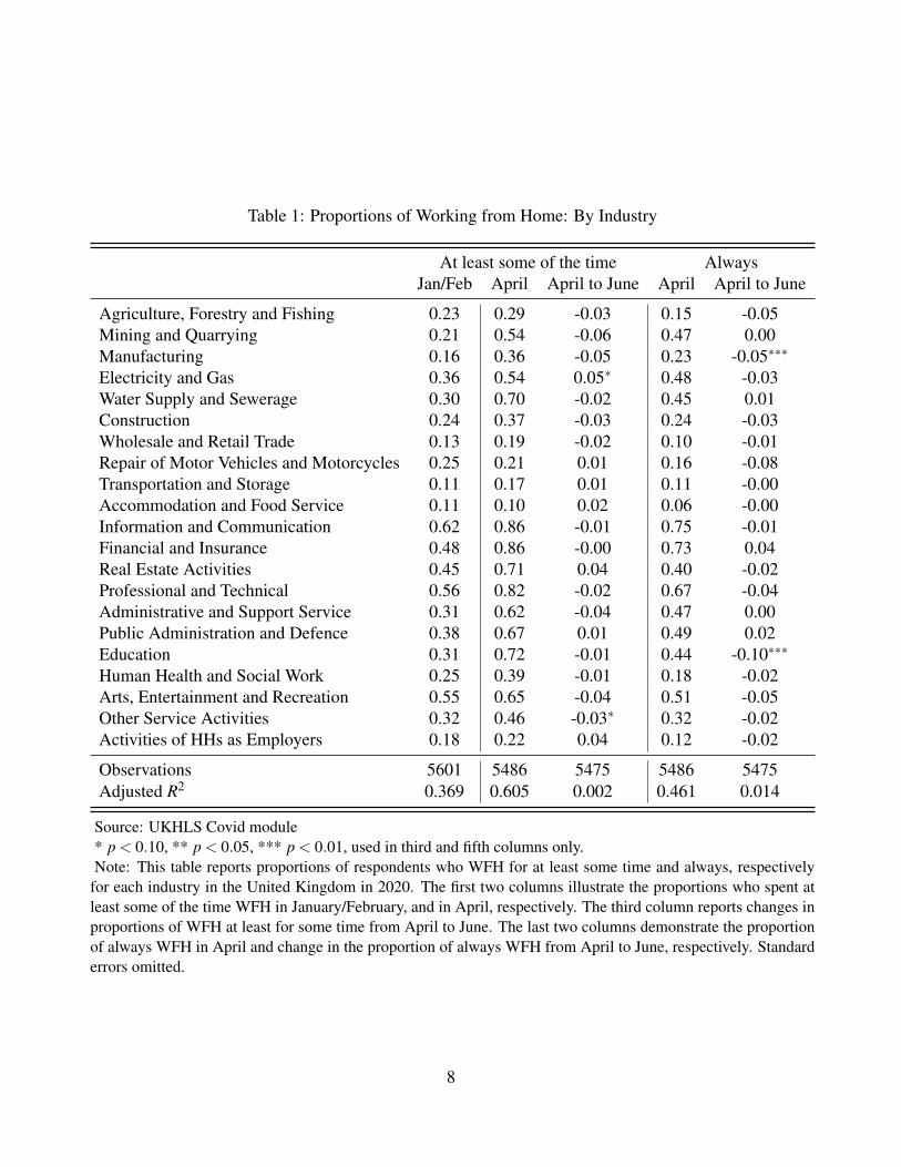
Table 1: Proportions of Working from Home: By Industry
At least some of the time AlwaysJan/Feb April April to June April April to June
Agriculture, Forestry and Fishing 0.23 0.29 -0.03 0.15 -0.05Mining and Quarrying 0.21 0.54 -0.06 0.47 0.00Manufacturing 0.16 0.36 -0.05 0.23 -0.05∗∗∗
Electricity and Gas 0.36 0.54 0.05∗ 0.48 -0.03Water Supply and Sewerage 0.30 0.70 -0.02 0.45 0.01Construction 0.24 0.37 -0.03 0.24 -0.03Wholesale and Retail Trade 0.13 0.19 -0.02 0.10 -0.01Repair of Motor Vehicles and Motorcycles 0.25 0.21 0.01 0.16 -0.08Transportation and Storage 0.11 0.17 0.01 0.11 -0.00Accommodation and Food Service 0.11 0.10 0.02 0.06 -0.00Information and Communication 0.62 0.86 -0.01 0.75 -0.01Financial and Insurance 0.48 0.86 -0.00 0.73 0.04Real Estate Activities 0.45 0.71 0.04 0.40 -0.02Professional and Technical 0.56 0.82 -0.02 0.67 -0.04Administrative and Support Service 0.31 0.62 -0.04 0.47 0.00Public Administration and Defence 0.38 0.67 0.01 0.49 0.02Education 0.31 0.72 -0.01 0.44 -0.10∗∗∗
Human Health and Social Work 0.25 0.39 -0.01 0.18 -0.02Arts, Entertainment and Recreation 0.55 0.65 -0.04 0.51 -0.05Other Service Activities 0.32 0.46 -0.03∗ 0.32 -0.02Activities of HHs as Employers 0.18 0.22 0.04 0.12 -0.02
Observations 5601 5486 5475 5486 5475Adjusted R2 0.369 0.605 0.002 0.461 0.014
Source: UKHLS Covid module* p < 0.10, ** p < 0.05, *** p < 0.01, used in third and fifth columns only.Note: This table reports proportions of respondents who WFH for at least some time and always, respectively
for each industry in the United Kingdom in 2020. The first two columns illustrate the proportions who spent atleast some of the time WFH in January/February, and in April, respectively. The third column reports changes inproportions of WFH at least for some time from April to June. The last two columns demonstrate the proportionof always WFH in April and change in the proportion of always WFH from April to June, respectively. Standarderrors omitted.
8
teachers worked away from home at least some of the time as schools partially reopened before thesummer vacation. Table B.1 shows proportions of working from home by occupation, using reportedoccupation from wave 9 of the main survey. Similar patterns are seen as with industry, with the majorchange from spring to summer in occupations relating to teaching.
3.2 Changes in Productivity by Basic Characteristics
We now document the changes in productivity reported in the June survey module, and for those work-ing at home at least some of the time. We first document average changes according to characteristicsof the worker. Our evidence is presented in Table 2. The table’s first column examines the relationshipbetween productivity changes and earnings, with workers split into terciles according to take home payacross the whole labour force in the baseline period. It seems the lowest earning group faced the worsedecline in productivity on average, while productivity of top earners has been boosted significantly.As discussed in Section 2, the data here come from an ordinal Likert scale. In Table 2, as in the restof the analysis, we construe responses as cardinal and interpret marginal effects in terms of standarddeviations away from no productivity change. We provide robustness to these results in Appendix Bwhere we perform the same analysis using ordered probits, with near identical results.
Despite the gradient by earnings, column two of Table 2 shows that on average productivity changesare not significantly dependent on degree holding itself. Although not shown here, productivity is alsonot noticeably different across age. The third column then illustrates a gender gap: on average femalesexperienced a significant productivity fall, whereas males were not noticeably impacted. A possiblecause for this is the unequal burden of home work, childcare and other distractions (Andrew et al.,2020). However, in terms of preliminary evidence here, the fourth column shows that productivity isnot noticeably affected by the presence of children, at least not across the population as a whole. Thefinal column shows that the self-employed group experiences a significantly worse productivity lossthan employees. One important reason is that many self-employed were already in their ideal workingenvironment before the pandemic, so they endured the negative effect of Covid, but did not feel thepositive effect of relocating to a more productive space. For example, in January 2020, already 24.2%of self-employed worked at home. Though the fraction increased to 36.4% in April 2020, the increaseis much smaller than that of the employed — from 3.8% to 34.5%.
To explore the gender divide in reported productivity in further detail, we present results brokendown by gender together with other characteristics in Table 3. Now columns 1 and 2 do indeed showan effect of the presence of children: females with childcare duty suffer a significant loss in productivity,while males are not so affected. This analysis demonstrates one of the strengths of our metric over and
9
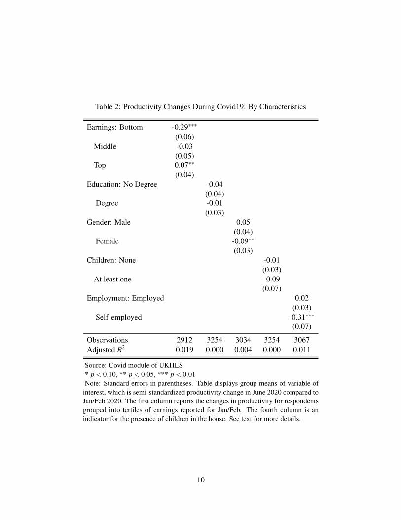
Table 2: Productivity Changes During Covid19: By Characteristics
Earnings: Bottom -0.29∗∗∗
(0.06)Middle -0.03
(0.05)Top 0.07∗∗
(0.04)Education: No Degree -0.04
(0.04)Degree -0.01
(0.03)Gender: Male 0.05
(0.04)Female -0.09∗∗
(0.03)Children: None -0.01
(0.03)At least one -0.09
(0.07)Employment: Employed 0.02
(0.03)Self-employed -0.31∗∗∗
(0.07)
Observations 2912 3254 3034 3254 3067Adjusted R2 0.019 0.000 0.004 0.000 0.011
Source: Covid module of UKHLS* p < 0.10, ** p < 0.05, *** p < 0.01Note: Standard errors in parentheses. Table displays group means of variable of
interest, which is semi-standardized productivity change in June 2020 compared toJan/Feb 2020. The first column reports the changes in productivity for respondentsgrouped into tertiles of earnings reported for Jan/Feb. The fourth column is anindicator for the presence of children in the house. See text for more details.
10
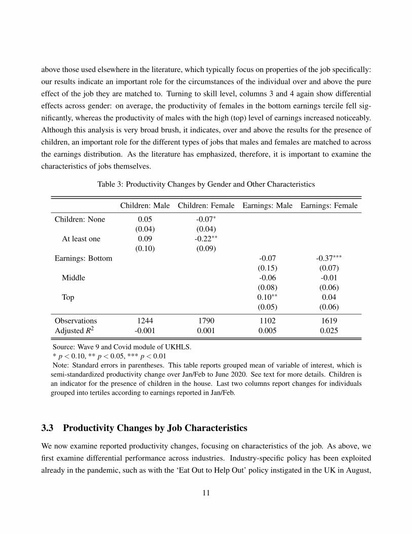
above those used elsewhere in the literature, which typically focus on properties of the job specifically:our results indicate an important role for the circumstances of the individual over and above the pureeffect of the job they are matched to. Turning to skill level, columns 3 and 4 again show differentialeffects across gender: on average, the productivity of females in the bottom earnings tercile fell sig-nificantly, whereas the productivity of males with the high (top) level of earnings increased noticeably.Although this analysis is very broad brush, it indicates, over and above the results for the presence ofchildren, an important role for the different types of jobs that males and females are matched to acrossthe earnings distribution. As the literature has emphasized, therefore, it is important to examine thecharacteristics of jobs themselves.
Table 3: Productivity Changes by Gender and Other Characteristics
Children: Male Children: Female Earnings: Male Earnings: Female
Children: None 0.05 -0.07∗
(0.04) (0.04)At least one 0.09 -0.22∗∗
(0.10) (0.09)Earnings: Bottom -0.07 -0.37∗∗∗
(0.15) (0.07)Middle -0.06 -0.01
(0.08) (0.06)Top 0.10∗∗ 0.04
(0.05) (0.06)
Observations 1244 1790 1102 1619Adjusted R2 -0.001 0.001 0.005 0.025
Source: Wave 9 and Covid module of UKHLS.* p < 0.10, ** p < 0.05, *** p < 0.01Note: Standard errors in parentheses. This table reports grouped mean of variable of interest, which is
semi-standardized productivity change over Jan/Feb to June 2020. See text for more details. Children isan indicator for the presence of children in the house. Last two columns report changes for individualsgrouped into tertiles according to earnings reported in Jan/Feb.
3.3 Productivity Changes by Job Characteristics
We now examine reported productivity changes, focusing on characteristics of the job. As above, wefirst examine differential performance across industries. Industry-specific policy has been exploitedalready in the pandemic, such as with the ‘Eat Out to Help Out’ policy instigated in the UK in August,
11
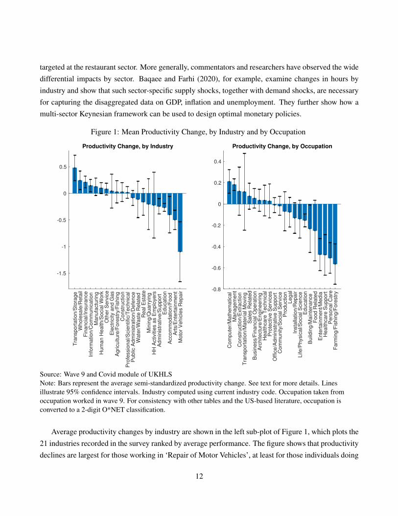
targeted at the restaurant sector. More generally, commentators and researchers have observed the widedifferential impacts by sector. Baqaee and Farhi (2020), for example, examine changes in hours byindustry and show that such sector-specific supply shocks, together with demand shocks, are necessaryfor capturing the disaggregated data on GDP, inflation and unemployment. They further show how amulti-sector Keynesian framework can be used to design optimal monetary policies.
Figure 1: Mean Productivity Change, by Industry and by Occupation
Productivity Change, by Industry
Tra
nsport
ation/S
tora
ge
Whole
sale
/Reta
ilF
inancia
l/In
sura
nce
Info
rmation/C
om
munic
ation
Manufa
ctu
ring
Hum
an H
ealth/S
ocia
l W
ork
Oth
er
Serv
ice
Ele
ctr
icity a
nd G
as
Agriculture
/Fore
str
y/F
ishin
gC
onstr
uction
Pro
fessio
nal/S
cie
ntific/T
echnic
al
Public
Adm
inis
tration/D
efe
nce
Wate
r/W
aste
Rela
ted
Real E
sta
teM
inin
g/Q
uarr
yin
g
HH
Activitie
s a
s E
mplo
yers
Adm
inis
trative/S
upport
E
ducation
Accom
modation/F
ood
Art
s/E
nte
rtain
ment
Moto
r V
ehic
les R
epair
-1.5
-1
-0.5
0
0.5
Productivity Change, by Occupation
Com
pute
r/M
ath
em
atical
Managem
ent
Constr
uction/E
xtr
action
Tra
nsport
ation/M
ate
rial M
ovin
gS
ale
s R
ela
ted
Busin
ess/F
inancia
l O
pera
tion
Arc
hitectu
re/E
ngin
eering
Healthcare
Technic
al
Pro
tective S
erv
ices
Offic
e/A
dm
inis
trative S
upport
Com
munity/S
ocia
l S
erv
ice
Pro
duction
Legal
Insta
llation/R
epair
Life/P
hysic
al/S
ocia
l S
cie
nce
Education
Build
ing/M
ain
tenance
Food R
ela
ted
Ente
rtain
ment/M
edia
Healthcare
Support
Pers
onal C
are
Farm
ing/F
ishin
g/F
ore
str
y
-0.8
-0.6
-0.4
-0.2
0
0.2
0.4
Source: Wave 9 and Covid module of UKHLSNote: Bars represent the average semi-standardized productivity change. See text for more details. Linesillustrate 95% confidence intervals. Industry computed using current industry code. Occupation taken fromoccupation worked in wave 9. For consistency with other tables and the US-based literature, occupation isconverted to a 2-digit O*NET classification.
Average productivity changes by industry are shown in the left sub-plot of Figure 1, which plots the21 industries recorded in the survey ranked by average performance. The figure shows that productivitydeclines are largest for those working in ‘Repair of Motor Vehicles’, at least for those individuals doing
12
some work from home. The magnitude of the decline is large, averaging one standard deviation ofthe entire distribution of reported changes. Other industries which show a decline that is statisticallysignificant include ‘Education’, which was transformed by the pandemic, and arts-related activities.This latter industry is an interesting case: While the realized productivity change in this industry isnegative (as reported both in our household data and official aggregate productivity statistics), jobcharacteristics themselves predict a large fraction of jobs in this industry can be done at home.
The left sub-plot of Figure 1 also shows industries for which workers report productivity increases.As one might expect, these include jobs in both the IT and finance sectors, which external metricsindicate require less face-to-face interaction. The other two sectors which report significant produc-tivity increases are trade, and transport and storage. Although jobs in these sectors are less able to beperformed at home than those in, say, IT, they do not require physical proximity to other individuals.These observations indicate that there are multiple reasons why productivity may change after work isre-arranged. Again we explore these points in further detail below.
The right sub-plot of Figure 1 shows average productivity changes by occupation. Here we takereported occupation stated in wave 9 as baseline and categorize workers using the 22 two-digit O*NETcodes. As explained in Appendix A, the two-digit O*NET codes are derived by using a cross-walk toconvert the 3-digit SOC 2000 codes contained in the UKHLS.4 Looking at the top of the sub-plot, theoccupation that shows the largest productivity increase, ‘Computer/Mathematical’, is similar to the ITindustrial sector in requiring little face-to-face interaction. The next occupation, ‘Management’, is aninteresting case, given that it is one of the job types requiring the most interaction on most measures.That managers report productivity increases is possibly very dependent on the current state of infor-mation technology. Very likely, if the pandemic had occurred 10 or 20 years previously, the rankingof occupations would look different. Looking at the bottom of the sub-plot, again some expectedoccupations, such as ‘Personal Care’, and ‘Education’ show productivity declines.
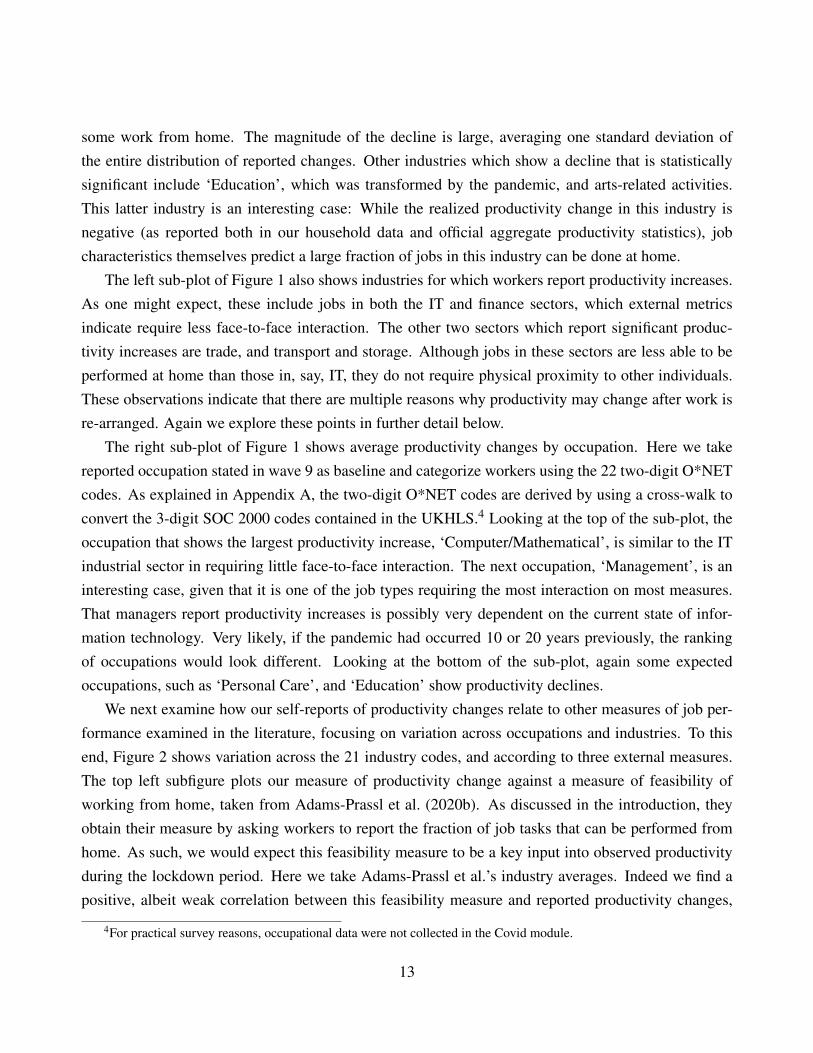
We next examine how our self-reports of productivity changes relate to other measures of job per-formance examined in the literature, focusing on variation across occupations and industries. To thisend, Figure 2 shows variation across the 21 industry codes, and according to three external measures.The top left subfigure plots our measure of productivity change against a measure of feasibility ofworking from home, taken from Adams-Prassl et al. (2020b). As discussed in the introduction, theyobtain their measure by asking workers to report the fraction of job tasks that can be performed fromhome. As such, we would expect this feasibility measure to be a key input into observed productivityduring the lockdown period. Here we take Adams-Prassl et al.’s industry averages. Indeed we find apositive, albeit weak correlation between this feasibility measure and reported productivity changes,
4For practical survey reasons, occupational data were not collected in the Covid module.
13
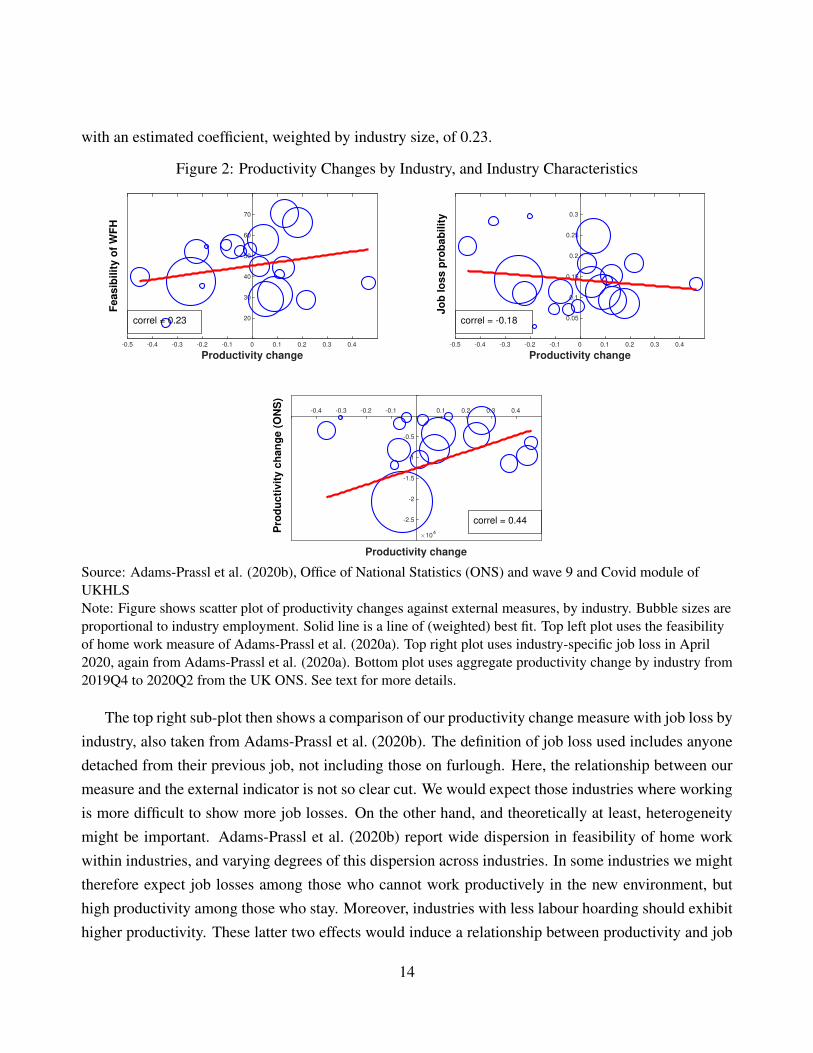
with an estimated coefficient, weighted by industry size, of 0.23.
Figure 2: Productivity Changes by Industry, and Industry Characteristics
-0.5 -0.4 -0.3 -0.2 -0.1 0 0.1 0.2 0.3 0.4
Productivity change
20
30
40
50
60
70
Feasib
ilit
y o
f W
FH
-0.5 -0.4 -0.3 -0.2 -0.1 0 0.1 0.2 0.3 0.4
Productivity change
0.05
0.1
0.15
0.2
0.25
0.3
Jo
b lo
ss p
rob
ab
ilit
y
-0.4 -0.3 -0.2 -0.1 0.1 0.2 0.3 0.4
Productivity change
-2.5
-2
-1.5
-1
-0.5
104P
rod
ucti
vit
y c
han
ge (
ON
S)
correl = 0.23 correl = -0.18
correl = 0.44
Source: Adams-Prassl et al. (2020b), Office of National Statistics (ONS) and wave 9 and Covid module ofUKHLSNote: Figure shows scatter plot of productivity changes against external measures, by industry. Bubble sizes areproportional to industry employment. Solid line is a line of (weighted) best fit. Top left plot uses the feasibilityof home work measure of Adams-Prassl et al. (2020a). Top right plot uses industry-specific job loss in April2020, again from Adams-Prassl et al. (2020a). Bottom plot uses aggregate productivity change by industry from2019Q4 to 2020Q2 from the UK ONS. See text for more details.
The top right sub-plot then shows a comparison of our productivity change measure with job loss byindustry, also taken from Adams-Prassl et al. (2020b). The definition of job loss used includes anyonedetached from their previous job, not including those on furlough. Here, the relationship between ourmeasure and the external indicator is not so clear cut. We would expect those industries where workingis more difficult to show more job losses. On the other hand, and theoretically at least, heterogeneitymight be important. Adams-Prassl et al. (2020b) report wide dispersion in feasibility of home workwithin industries, and varying degrees of this dispersion across industries. In some industries we mighttherefore expect job losses among those who cannot work productively in the new environment, buthigh productivity among those who stay. Moreover, industries with less labour hoarding should exhibithigher productivity. These latter two effects would induce a relationship between productivity and job
14
loss that is positive. Overall, however, we do see a negative correlation between job losses and reportedproductivity, albeit a weak one.
Finally, the bottom sub-plot of Figure 2 compares our self-reported productivity changes with offi-cial aggregate productivity by industry reported by the ONS.5 For better comparison with the externalmeasure, here we compute a measure of industry-level aggregate productivity change. We do this byweighting the reported changes by earnings reported in January. This weighted correlation coefficientis higher than those in the top two panels, at 0.44. Of course, the discrepancy between our measure andofficial productivity may be caused by any number of factors. These include biases in self-reporting,and the fact that our data omits those still always working outside the home.
We show variation by occupation in Figure 3.6 Whereas our industry measure captures currentwork status, our measure of occupation is taken from wave 9, just before the pandemic. Nevertheless,this measure should capture baseline occupation well; the available evidence suggests there was littlenoticeable rise in occupational mobility during the Covid-19 period (Office for National Statistics,2020). As discussed above and in Section 2, the occupational information in UKHLS is provided at the3-digit SOC 2000 level. In order to compare to measures in the literature we convert to 2-digit O*NEToccupations using the cross-walk described in Appendix A.
The top left panel again shows a comparison with feasibility of working from home, taken fromAdams-Prassl et al. (2020b). Compared to the equivalent subpanel in Figure 2, the correlation be-tween our measure and the external measure is now stronger, at 0.56. This is perhaps to be expected:feasibility of working from home presumably depends more on occupational rather than on industrialcharacteristics. The top right sub-plot of Figure 3 also shows the equivalent panel to that shown previ-ously, plotting productivity change against job losses. Now the negative correlation with productivitychanges is particularly strong, at -0.67. This indicates that it is at the occupation level that productivitychanges determine job losses, rather than at the industry sector level.
The bottom sub-plot of Figure 3 now introduces another metric discussed in the literature thatshould be related to productivity. It compares our reported changes to a measure of need for physicalproximity with others, derived by Mongey et al. (2020) using O*NET descriptors. Again these mea-sures are reported by the authors at the 2-digit O*NET occupation level. Those occupations which areindicated to require close physical interaction between workers, such as ‘Personal Care’ and ‘Health-
5The ONS combines three industries, ‘Public Administration and Defense’, ‘Education’, and ‘Human Healthand Social Work Activities’ into one category and also combines ‘Other Service Activities’ and ‘Activities ofHouseholds as Employers’ into another category. Therefore, for consistency, we combine our industry datasimilarly.
6In this figure, the category ‘Farming, Fishing, and Forestry Occupations’ is dropped, for comparability withAdams-Prassl et al. (2020b).
15
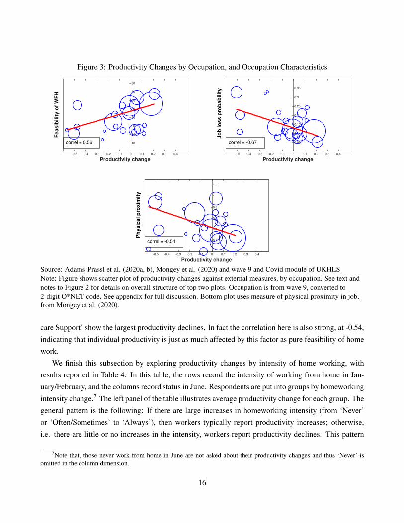
Figure 3: Productivity Changes by Occupation, and Occupation Characteristics
-0.5 -0.4 -0.3 -0.2 -0.1 0 0.1 0.2 0.3 0.4
Productivity change
10
20
30
40
50
60
70
80
Feasib
ilit
y o
f W
FH
-0.5 -0.4 -0.3 -0.2 -0.1 0 0.1 0.2 0.3 0.4
Productivity change
0.05
0.1
0.15
0.2
0.25
0.3
0.35
Jo
b lo
ss p
rob
ab
ilit
y
-0.5 -0.4 -0.3 -0.2 -0.1 0 0.1 0.2 0.3 0.4
Productivity change
0.2
0.4
0.6
0.8
1
1.2
Ph
ysic
al p
roxim
ity
correl = 0.56 correl = -0.67
correl = -0.54
Source: Adams-Prassl et al. (2020a, b), Mongey et al. (2020) and wave 9 and Covid module of UKHLSNote: Figure shows scatter plot of productivity changes against external measures, by occupation. See text andnotes to Figure 2 for details on overall structure of top two plots. Occupation is from wave 9, converted to2-digit O*NET code. See appendix for full discussion. Bottom plot uses measure of physical proximity in job,from Mongey et al. (2020).
care Support’ show the largest productivity declines. In fact the correlation here is also strong, at -0.54,indicating that individual productivity is just as much affected by this factor as pure feasibility of homework.
We finish this subsection by exploring productivity changes by intensity of home working, withresults reported in Table 4. In this table, the rows record the intensity of working from home in Jan-uary/February, and the columns record status in June. Respondents are put into groups by homeworkingintensity change.7 The left panel of the table illustrates average productivity change for each group. Thegeneral pattern is the following: If there are large increases in homeworking intensity (from ‘Never’or ‘Often/Sometimes’ to ‘Always’), then workers typically report productivity increases; otherwise,i.e. there are little or no increases in the intensity, workers report productivity declines. This pattern
7Note that, those never work from home in June are not asked about their productivity changes and thus ‘Never’ isomitted in the column dimension.
16
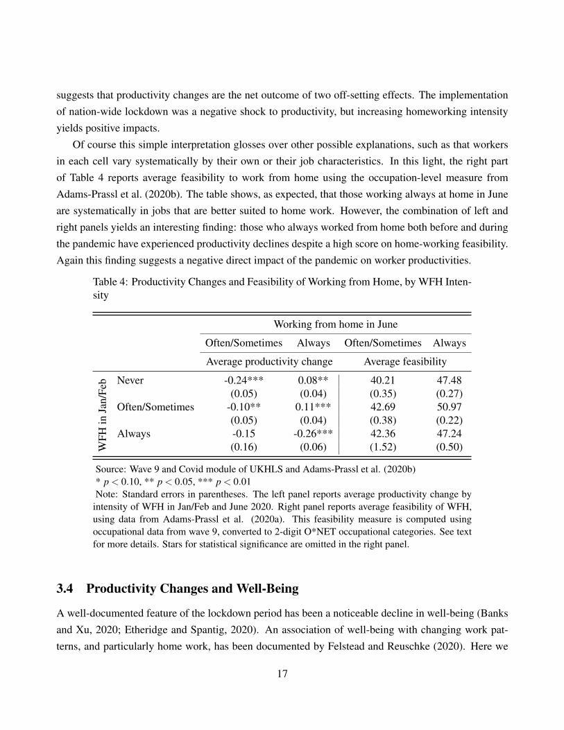
suggests that productivity changes are the net outcome of two off-setting effects. The implementationof nation-wide lockdown was a negative shock to productivity, but increasing homeworking intensityyields positive impacts.
Of course this simple interpretation glosses over other possible explanations, such as that workersin each cell vary systematically by their own or their job characteristics. In this light, the right partof Table 4 reports average feasibility to work from home using the occupation-level measure fromAdams-Prassl et al. (2020b). The table shows, as expected, that those working always at home in Juneare systematically in jobs that are better suited to home work. However, the combination of left andright panels yields an interesting finding: those who always worked from home both before and duringthe pandemic have experienced productivity declines despite a high score on home-working feasibility.Again this finding suggests a negative direct impact of the pandemic on worker productivities.
Table 4: Productivity Changes and Feasibility of Working from Home, by WFH Inten-sity
Working from home in June
Often/Sometimes Always Often/Sometimes Always
Average productivity change Average feasibility
WFH
inJa
n/Fe
b Never -0.24*** 0.08** 40.21 47.48(0.05) (0.04) (0.35) (0.27)
Often/Sometimes -0.10** 0.11*** 42.69 50.97(0.05) (0.04) (0.38) (0.22)
Always -0.15 -0.26*** 42.36 47.24(0.16) (0.06) (1.52) (0.50)
Source: Wave 9 and Covid module of UKHLS and Adams-Prassl et al. (2020b)* p < 0.10, ** p < 0.05, *** p < 0.01Note: Standard errors in parentheses. The left panel reports average productivity change by
intensity of WFH in Jan/Feb and June 2020. Right panel reports average feasibility of WFH,using data from Adams-Prassl et al. (2020a). This feasibility measure is computed usingoccupational data from wave 9, converted to 2-digit O*NET occupational categories. See textfor more details. Stars for statistical significance are omitted in the right panel.
3.4 Productivity Changes and Well-Being
A well-documented feature of the lockdown period has been a noticeable decline in well-being (Banksand Xu, 2020; Etheridge and Spantig, 2020). An association of well-being with changing work pat-terns, and particularly home work, has been documented by Felstead and Reuschke (2020). Here we
17
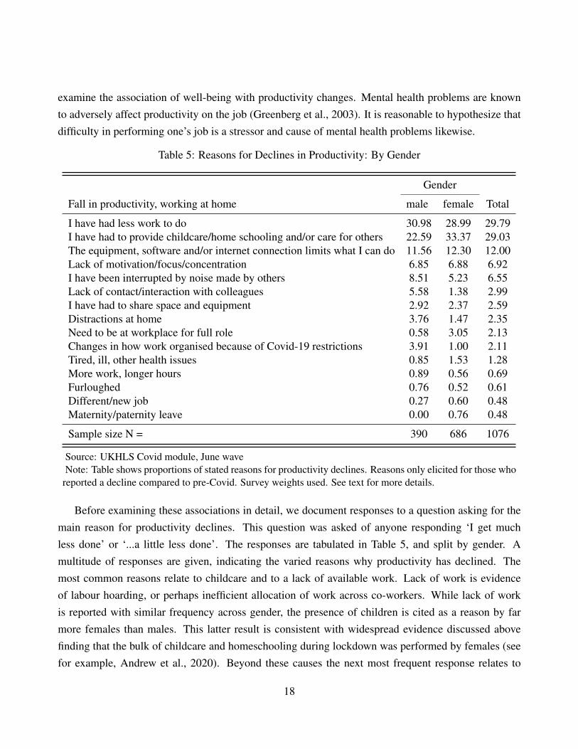
examine the association of well-being with productivity changes. Mental health problems are knownto adversely affect productivity on the job (Greenberg et al., 2003). It is reasonable to hypothesize thatdifficulty in performing one’s job is a stressor and cause of mental health problems likewise.
Table 5: Reasons for Declines in Productivity: By Gender
Gender
Fall in productivity, working at home male female Total
I have had less work to do 30.98 28.99 29.79I have had to provide childcare/home schooling and/or care for others 22.59 33.37 29.03The equipment, software and/or internet connection limits what I can do 11.56 12.30 12.00Lack of motivation/focus/concentration 6.85 6.88 6.92I have been interrupted by noise made by others 8.51 5.23 6.55Lack of contact/interaction with colleagues 5.58 1.38 2.99I have had to share space and equipment 2.92 2.37 2.59Distractions at home 3.76 1.47 2.35Need to be at workplace for full role 0.58 3.05 2.13Changes in how work organised because of Covid-19 restrictions 3.91 1.00 2.11Tired, ill, other health issues 0.85 1.53 1.28More work, longer hours 0.89 0.56 0.69Furloughed 0.76 0.52 0.61Different/new job 0.27 0.60 0.48Maternity/paternity leave 0.00 0.76 0.48
Sample size N = 390 686 1076
Source: UKHLS Covid module, June waveNote: Table shows proportions of stated reasons for productivity declines. Reasons only elicited for those who
reported a decline compared to pre-Covid. Survey weights used. See text for more details.
Before examining these associations in detail, we document responses to a question asking for themain reason for productivity declines. This question was asked of anyone responding ‘I get muchless done’ or ‘...a little less done’. The responses are tabulated in Table 5, and split by gender. Amultitude of responses are given, indicating the varied reasons why productivity has declined. Themost common reasons relate to childcare and to a lack of available work. Lack of work is evidenceof labour hoarding, or perhaps inefficient allocation of work across co-workers. While lack of workis reported with similar frequency across gender, the presence of children is cited as a reason by farmore females than males. This latter result is consistent with widespread evidence discussed abovefinding that the bulk of childcare and homeschooling during lockdown was performed by females (seefor example, Andrew et al., 2020). Beyond these causes the next most frequent response relates to
18
lack of adequate equipment or software at home. Further down the list, the only reasons quoted bya non-negligible fraction of respondents are a lack of motivation, and noise distractions by others,presumably other than children. The former reason most directly indicates a causal effect from mentalhealth declines. Reports of noise distractions further indicate the stressful situations under which someworkers were required to perform their jobs.
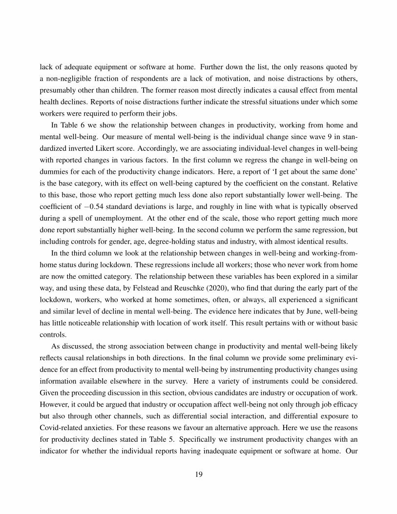
In Table 6 we show the relationship between changes in productivity, working from home andmental well-being. Our measure of mental well-being is the individual change since wave 9 in stan-dardized inverted Likert score. Accordingly, we are associating individual-level changes in well-beingwith reported changes in various factors. In the first column we regress the change in well-being ondummies for each of the productivity change indicators. Here, a report of ‘I get about the same done’is the base category, with its effect on well-being captured by the coefficient on the constant. Relativeto this base, those who report getting much less done also report substantially lower well-being. Thecoefficient of −0.54 standard deviations is large, and roughly in line with what is typically observedduring a spell of unemployment. At the other end of the scale, those who report getting much moredone report substantially higher well-being. In the second column we perform the same regression, butincluding controls for gender, age, degree-holding status and industry, with almost identical results.
In the third column we look at the relationship between changes in well-being and working-from-home status during lockdown. These regressions include all workers; those who never work from homeare now the omitted category. The relationship between these variables has been explored in a similarway, and using these data, by Felstead and Reuschke (2020), who find that during the early part of thelockdown, workers, who worked at home sometimes, often, or always, all experienced a significantand similar level of decline in mental well-being. The evidence here indicates that by June, well-beinghas little noticeable relationship with location of work itself. This result pertains with or without basiccontrols.
As discussed, the strong association between change in productivity and mental well-being likelyreflects causal relationships in both directions. In the final column we provide some preliminary evi-dence for an effect from productivity to mental well-being by instrumenting productivity changes usinginformation available elsewhere in the survey. Here a variety of instruments could be considered.Given the proceeding discussion in this section, obvious candidates are industry or occupation of work.However, it could be argued that industry or occupation affect well-being not only through job efficacybut also through other channels, such as differential social interaction, and differential exposure toCovid-related anxieties. For these reasons we favour an alternative approach. Here we use the reasonsfor productivity declines stated in Table 5. Specifically we instrument productivity changes with anindicator for whether the individual reports having inadequate equipment or software at home. Our
19
Table 6: Productivity Changes, Working from Home, and Mental Well-Being
Change in well-being
OLS OLS OLS OLS IV
Prod. change (index) 0.24∗∗∗
(0.07)Prod: much less done -0.54∗∗∗ -0.58∗∗∗
(0.12) (0.10)Get little less done -0.25∗∗∗ -0.24∗∗∗
(0.07) (0.07)Get little more done 0.02 0.05
(0.07) (0.07)Get much more done 0.30∗∗∗ 0.30∗∗∗
(0.08) (0.08)Working from Home: Always -0.03 0.01
(0.04) (0.05)Often -0.04 -0.01
(0.07) (0.07)Sometimes -0.06 -0.06
(0.09) (0.09)Constant -0.20∗∗∗ -0.16 -0.23∗∗∗ 1.64∗∗∗ -0.08
(0.04) (0.19) (0.03) (0.11) (0.22)
Observations 3190 2957 6024 5513 2957ControlsAdjusted R2 0.043 0.084 -0.000 0.024 0.081
Source: Wave 9 and Covid module of UKHLS* p < 0.10,** p < 0.05, *** p < 0.01Note: Standard errors in parentheses. In column 5, productivity change is instrumented with
report of having ineffective equipment. In columns 2, 4 and 5, regressions include followingcontrols: respondent’s gender, age, education level (degree holding) and job industry. Incolumn 3 and 4, we report relationship between mental wellbeing and WFH intensity usingJune wave of UKHLS Covid module.
20
maintained hypothesis is that lack of equipment only affects change in well-being through its effecton productivity. A possible criticism of this approach is that, given that the reasons for productivitychanges are never elicited from those who report productivity increases, then the ‘first-stage’ regres-sion is ensured by construction. Nevertheless we feel it is realistic to assume that those who experienceequipment problems do find it detrimental on average. Turning to results, we find (but do not show)that those reporting inadequate equipment indeed suffer declines in well-being. Accordingly, and interms of an IV regression, the fifth column of Table 6 shows that the effect of productivity changes onwell-being is strong.
4 Conclusion
The Covid-19 pandemic has caused widespread disruption to working practices. The most noticeablechange has been the vast increase in working from home. While some changes to working practicesare probably temporary, many could very likely be persistent. Even after the pandemic ends, homeworking in particular is expected to be much more prevalent than previously.
In this paper we use the Covid-19 module from a household panel in the UK, which provides repre-sentative data on home workers’ self-reported productivity towards the end of the lock-down period, inJune 2020. In this survey, anyone working from home (WFH) at least some of the time was asked aboutchanges in their productivity since before the pandemic period, at the beginning of the year. These dataallow us to examine how productivity changes vary across both job and worker types.
We find that workers in industries and occupations that are less suitable for working from homereport lower productivities than before the pandemic. Consistently with this, and with the literature,females and low earners also report lower productivity at home on average. For females, this lowerproductivity is not only due to the average characteristics of their jobs, but also because they are dis-proportionately effected by the presence of children. When examining workers based on changes intheir WFH intensity, the evidence suggests that working from home itself has largely been beneficial,and has offset the other negative effects of the pandemic on productivity. Finally we produce evidencesuggesting that difficulty in performing one’s job causes lower mental well-being.
The evidence provided in this paper is relevant for policy in several ways. Most importantly itcontributes to our understanding of the sector-specific impacts of the pandemic. This in turn helpsinform policy-makers of the likely efficacy of targeted policies. It also informs quantitative analysesinvolving models of sector-specific supply shocks.
21
ReferencesADAMS-PRASSL, A., T. BONEVA, M. GOLIN, AND C. RAUH (2020a): “Inequality in the Impact of the Coronavirus
Shock: Evidence from Real Time Surveys,” Journal of Public Economics, 189.
——— (2020b): “Work That Can Be Done from Home: Evidence on Variation within and across Occupations and Indus-tries,” .
ALON, T., M. DOEPKE, J. OLMSTEAD-RUMSEY, AND M. TERTILT (2020): “The Impact of COVID-19 on Gender Equal-ity,” .
ANDREW, A., S. CATTAN, M. COSTA DIAS, C. FARQUHARSON, L. KRAFTMAN, S. KRUTIKOVA, A. PHIMISTER, AND
A. SEVILLA (2020): “How Are Mothers and Fathers Balancing Work and Family under Lockdown?” Tech. rep., TheInstitute for Fiscal Studies.
BANKS, J. AND X. XU (2020): “The mental health effects of the first two months of lockdown and social distancing duringthe Covid-19 pandemic in the UK,” Covid Economics, 28, 91–118.
BAQAEE, D. R. AND E. FARHI (2020): “Supply and Demand in Disaggregated Keynesian Economies with an Applicationto the COVID-19 Crisis,” .
BLOOM, B. N. (2020): “How Working from Home Works out,” Tech. rep.
BLOOM, N., J. LIANG, J. ROBERTS, AND Z. J. YING (2015): “Does Working from Home Work? Evidence from a ChineseExperiment,” The Quarterly Journal of Economics, 130, 165–218.
BLUNDELL, R. AND B. ETHERIDGE (2010): “Consumption, Income and Earnings Inequality in Britain,” Review of Eco-nomic Dynamics, 13, 76–102.
BLUNDELL, R., D. A. GREEN, AND W. JIN (2016): “The UK Wage Premium Puzzle: How Did a Large Increase inUniversity Graduates Leave the Education Premium Unchanged?” .
BONADIO, B., Z. HUO, A. LEVCHENKO, AND N. PANDALAI-NAYAR (2020): “Global Supply Chains in the Pandemic,”NBER Working Paper.
BRODEUR, A., A. CLARK, S. FLECHE, AND N. POWDTHAVEE (2020): “Assessing the Impact of the Coronavirus Lock-down on Unhappiness, Loneliness, and Boredom Using Google Trends,” .
BROOKS, S. K., R. WEBSTER, L. E. SMITH, L. WOODLAND, S. WESSELY, N. GREENBERG, AND G. J. RUBIN (2020):“The Psychological Impact of Quarantine and How to Reduce It: Rapid Review of the Evidence,” The Lancet, 395,912–920.
BRYNJOLFSSON, E., J. J. HORTON, A. OZIMEK, D. ROCK, G. SHARMA, H.-Y. TUYE, AND A. O. UPWORK (2020):“COVID-19 and Remote Work: An Early Look at US Data,” .
CHANG, S. S., D. STUCKLER, P. YIP, AND D. GUNNELL (2013): “Impact of 2008 Global Economic Crisis on Suicide:Time Trend Study in 54 Countries,” BMJ, 347, 1–15.
22
DAGHER, R. K., J. CHEN, AND S. B. THOMAS (2015): “Gender Differences in Mental Health Outcomes before, during,and after the Great Recession,” PLoS ONE, 10, 1–16.
DINGEL, J. I. AND B. NEIMAN (2020): “How Many Jobs Can Be Done at Home?” Journal of Public Economics, 189.
ETHERIDGE, B. AND L. SPANTIG (2020): “The Gender Gap in Mental Well-Being during the COVID-19 Outbreak:Evidence from the UK,” .
EUROFOUND (2020): “Living, Working and COVID-19 - First Findings,” Tech. rep.
FELSTEAD, A. AND D. REUSCHKE (2020): “Homeworking in the UK: Before and during the 2020 Lockdown,” Tech. rep.
FETZER, T., L. HENSEL, J. HERMLE, AND C. ROTH (2020): “Coronavirus Perceptions and Economic Anxiety,” Reviewof Economics and Statistics, forthcomin.
GREENBERG, P. E., R. C. KESSLER, H. G. BIRNBAUM, S. A. LEONG, S. W. LOWE, P. A. BERGLUND, AND P. K.COREY-LISLE (2003): “The Economic Burden of Depression in the United States: How Did It Change between 1990and 2000?” Journal of Clinical Psychiatry, 64, 1465–1475.
HEATHCOTE, J., F. PERRI, AND G. L. VIOLANTE (2010): “Unequal We Stand: An Empirical Analysis of EconomicInequality in the United States, 1967-2006,” Review of Economic Dynamics, 13, 15–51.
HOLMES, E. A., R. C. O’CONNOR, V. H. PERRY, I. TRACEY, S. WESSELY, L. ARSENEAULT, C. BALLARD, H. CHRIS-TENSEN, R. COHEN SILVER, I. EVERALL, T. FORD, A. JOHN, T. KABIR, K. KING, I. MADAN, S. MICHIE, A. K.PRZYBYLSKI, R. SHAFRAN, A. SWEENEY, C. M. WORTHMAN, L. YARDLEY, K. COWAN, C. COPE, M. HOTOPF,AND E. BULLMORE (2020): “Multidisciplinary Research Priorities for the COVID-19 Pandemic: A Call for Action forMental Health Science,” The Lancet Psychiatry, 7, 547–560.
INSTITUTE FOR SOCIAL AND ECONOMIC RESEARCH (2020): “Understanding Society: COVID-19 Study,” SN: 8644,10.5255/UKDA–SN–8644–1.
JANKE, K., K. LEE, C. PROPPER, K. SHIELDS, AND M. A. SHIELDS (2020): “Macroeconomic Conditions and Health inBritain: Aggregation, Dynamics and Local Area Heterogeneity,” .
KNIPE, D., H. EVANS, A. MARCHANT, D. GUNNELL, AND A. JOHN (2020): “Mapping Population Mental HealthConcerns Related to COVID-19 and the Consequences of Physical Distancing: A Google Trends Analysis,” WellcomeOpen Research, 5.
MONGEY, S., L. PILOSSOPH, AND A. WEINBERG (2020): “Which Workers Bear the Burden of Social Distancing Poli-cies?” .
OFFICE FOR NATIONAL STATISTICS (2020): “Coronavirus and Occupational Switching: January to June 2020,” Tech. rep.
PERRI, F. AND J. STEINBERG (2012): “Inequality and Redistribution during the Great Recession,” .
RUBIN, O., A. NIKOLAEVA, S. NELLO-DEAKIN, AND M. TE BROMMELSTROET (2020): “What Can We Learn from theCOVID-19 Pandemic about How People Experience Working from Home and Commuting?” Tech. rep.
23

TUBADJI, A., F. BOY, AND D. J. WEBBER (2020): “Narrative Economics, Public Policy and Mental Health,” .
WORLD HEALTH ORGANIZATION (2020): “Mental Health and Psychosocial Considerations during COVID-19 Outbreak,”Tech. rep.
24
Appendix
A Cross-walk between SOC 2000 and O*NET Occupation
Table A.1 shows the cross-walk this paper adopts to convert the Standard Occupational Classification(SOC) 2000 to the Occupational Information Network (O*NET) codes. Specifically, we assign each3-digit SOC (sub-major occupation groups) into 2-digit O*NET codes (major occupation groups) bylooking into the 4-digit SOC (sub-sub-major occupation groups) under each 3-digit SOC classificationand matching them (4-digit SOC) with the most appropriate 2-digit O*NET category. Then, we assigneach 3-digit SOC, based on the matching outcomes of 4-digit SOC to 2-digit O*NET code using anemployment-weighted majority rule. Further, we also utilize industry information to split occupationsunder 3-digit SOC. Specifically, under SOC 922 ‘Elementary Personal Services Occupations’, severalfood preparation related occupations are listed, such as ‘Kitchen and catering assistants’, ‘Waiters
and Waitresses’. These occupations belong to the industry related to food. Therefore, we move thoserespondents whose 3-digit SOC is 922 and industry related to Food into O*NET 35 ‘Food Preparation
and Serving Related Occupations’.
Although in most cases the overwhelming majority of 4-digit SOC codes are assigned to the same2-digit O*NET code, this is not always the case. As a result, some matches between SOC 2000 andO*NET codes are necessarily imprecise. For instance, SOC 231 ‘Teaching Professionals’ is classifiedinto O*NET 25 ‘Education, Training, and Library Occupations’, yet under it, SOC 2317 ‘Registrars
and senior administrators of educational establishments’ is more appropriate to be put into 2-digitO*NET 11 ‘Management Occupations’, according to O*NET description. Due to the unavailabilityof 4-digit SOC information, we are unable to specifically subtract sub-sub-major occupation groupSOC 2317 from sub-major occupation group SOC 231. Similarly, we cannot move SOC 5241 ‘Elec-
tricians’ out of O*NET 49 ‘Installation, Maintenance, and Repair Occupations’ and into O*NET 47‘Construction and Extraction Occupations’.
Figure A.1 plots occupation distributions of respondents from wave 9 and the Covid module of UKHousehold Longitudinal Study (UKHLS) and national employment statistics from 2019 US Bureau ofLabor Statistics (BLS).
In the figure, white columns represent occupation percentages in UK-HLS and grey columns rep-
25
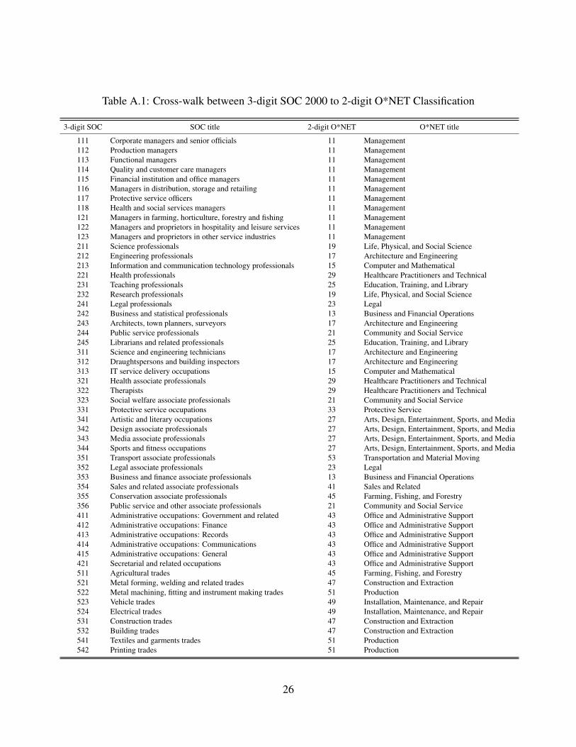
Table A.1: Cross-walk between 3-digit SOC 2000 to 2-digit O*NET Classification
3-digit SOC SOC title 2-digit O*NET O*NET title
111 Corporate managers and senior officials 11 Management112 Production managers 11 Management113 Functional managers 11 Management114 Quality and customer care managers 11 Management115 Financial institution and office managers 11 Management116 Managers in distribution, storage and retailing 11 Management117 Protective service officers 11 Management118 Health and social services managers 11 Management121 Managers in farming, horticulture, forestry and fishing 11 Management122 Managers and proprietors in hospitality and leisure services 11 Management123 Managers and proprietors in other service industries 11 Management211 Science professionals 19 Life, Physical, and Social Science212 Engineering professionals 17 Architecture and Engineering213 Information and communication technology professionals 15 Computer and Mathematical221 Health professionals 29 Healthcare Practitioners and Technical231 Teaching professionals 25 Education, Training, and Library232 Research professionals 19 Life, Physical, and Social Science241 Legal professionals 23 Legal242 Business and statistical professionals 13 Business and Financial Operations243 Architects, town planners, surveyors 17 Architecture and Engineering244 Public service professionals 21 Community and Social Service245 Librarians and related professionals 25 Education, Training, and Library311 Science and engineering technicians 17 Architecture and Engineering312 Draughtspersons and building inspectors 17 Architecture and Engineering313 IT service delivery occupations 15 Computer and Mathematical321 Health associate professionals 29 Healthcare Practitioners and Technical322 Therapists 29 Healthcare Practitioners and Technical323 Social welfare associate professionals 21 Community and Social Service331 Protective service occupations 33 Protective Service341 Artistic and literary occupations 27 Arts, Design, Entertainment, Sports, and Media342 Design associate professionals 27 Arts, Design, Entertainment, Sports, and Media343 Media associate professionals 27 Arts, Design, Entertainment, Sports, and Media344 Sports and fitness occupations 27 Arts, Design, Entertainment, Sports, and Media351 Transport associate professionals 53 Transportation and Material Moving352 Legal associate professionals 23 Legal353 Business and finance associate professionals 13 Business and Financial Operations354 Sales and related associate professionals 41 Sales and Related355 Conservation associate professionals 45 Farming, Fishing, and Forestry356 Public service and other associate professionals 21 Community and Social Service411 Administrative occupations: Government and related 43 Office and Administrative Support412 Administrative occupations: Finance 43 Office and Administrative Support413 Administrative occupations: Records 43 Office and Administrative Support414 Administrative occupations: Communications 43 Office and Administrative Support415 Administrative occupations: General 43 Office and Administrative Support421 Secretarial and related occupations 43 Office and Administrative Support511 Agricultural trades 45 Farming, Fishing, and Forestry521 Metal forming, welding and related trades 47 Construction and Extraction522 Metal machining, fitting and instrument making trades 51 Production523 Vehicle trades 49 Installation, Maintenance, and Repair524 Electrical trades 49 Installation, Maintenance, and Repair531 Construction trades 47 Construction and Extraction532 Building trades 47 Construction and Extraction541 Textiles and garments trades 51 Production542 Printing trades 51 Production
26
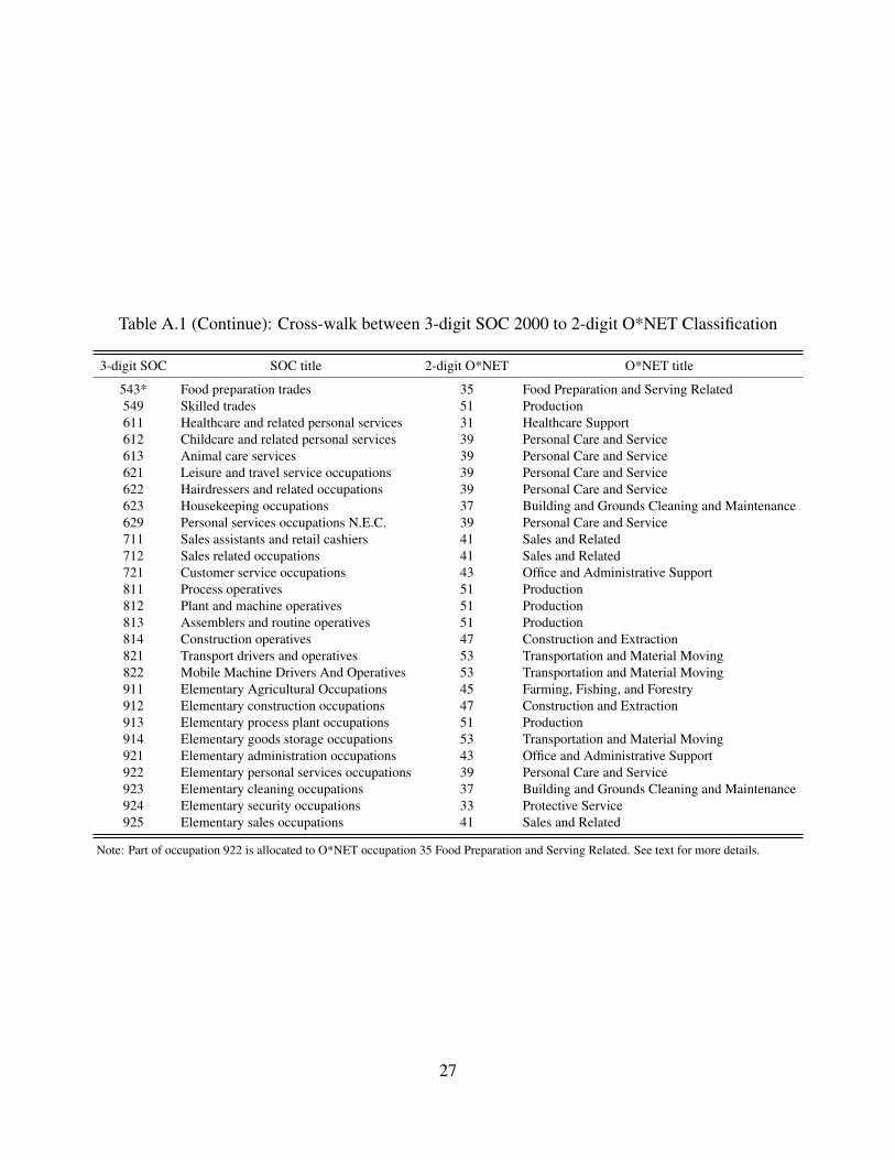
Table A.1 (Continue): Cross-walk between 3-digit SOC 2000 to 2-digit O*NET Classification
3-digit SOC SOC title 2-digit O*NET O*NET title
543* Food preparation trades 35 Food Preparation and Serving Related549 Skilled trades 51 Production611 Healthcare and related personal services 31 Healthcare Support612 Childcare and related personal services 39 Personal Care and Service613 Animal care services 39 Personal Care and Service621 Leisure and travel service occupations 39 Personal Care and Service622 Hairdressers and related occupations 39 Personal Care and Service623 Housekeeping occupations 37 Building and Grounds Cleaning and Maintenance629 Personal services occupations N.E.C. 39 Personal Care and Service711 Sales assistants and retail cashiers 41 Sales and Related712 Sales related occupations 41 Sales and Related721 Customer service occupations 43 Office and Administrative Support811 Process operatives 51 Production812 Plant and machine operatives 51 Production813 Assemblers and routine operatives 51 Production814 Construction operatives 47 Construction and Extraction821 Transport drivers and operatives 53 Transportation and Material Moving822 Mobile Machine Drivers And Operatives 53 Transportation and Material Moving911 Elementary Agricultural Occupations 45 Farming, Fishing, and Forestry912 Elementary construction occupations 47 Construction and Extraction913 Elementary process plant occupations 51 Production914 Elementary goods storage occupations 53 Transportation and Material Moving921 Elementary administration occupations 43 Office and Administrative Support922 Elementary personal services occupations 39 Personal Care and Service923 Elementary cleaning occupations 37 Building and Grounds Cleaning and Maintenance924 Elementary security occupations 33 Protective Service925 Elementary sales occupations 41 Sales and Related
Note: Part of occupation 922 is allocated to O*NET occupation 35 Food Preparation and Serving Related. See text for more details.
27
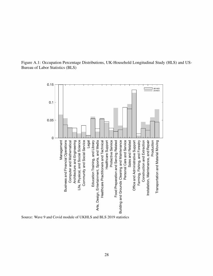
Figure A.1: Occupation Percentage Distributions, UK-Household Longitudinal Study (HLS) and US-Bureau of Labor Statistics (BLS)
Source: Wave 9 and Covid module of UKHLS and BLS 2019 statistics
28
resent occupation percentages in US-BLS. The correlation coefficient between both is around 0.7. Theoccupation categories showing largest differences are Management and Food Preparation and ServingRelated. The sign of these differences is, at least, very likely genuine. The UK is reported to beparticularly intensive in managers (Blundell et al., 2016). Similarly, the US is more intensive in FoodServing (waitering). If we exclude these occupations, the correlation coefficient between UK and USoccupation percentage rises to around 0.8.
B Additional Information and Results
B.1 Productivity Data from the ONS
We also utilize the productivity statistics reported by Office for National Statistics (ONS) in each in-dustry in UK. The productivity measures cover from 1997 Q2 to 2020 Q2 for UK main industries.Three seasonally adjusted statistics related to industry-level productivity are reported: gross valueadded (GVA), hours worked and output per hour. Both GVA and output per hour are measured by 2016GBP. The relationship between these three statistics is: GVA equals the product of hours worked andoutput per hour. Further, we derive the industry-level productivity changes by calculating the differenceof GVA between 2020 Q2 and 2019 Q4 for each industry. Note that, since for Manufacture industry,13 sub-industry statistics are reported separately, e.g. Manufacture of food products, beverages andtobacco and Manufacture of textiles, wearing apparel and leather products, we obtain Manufacture-level GVA by aggregating sub-industries through calculating the product of hours worked and outputper hour for all 13 individual sub-industries and then summing the 13 products up. The industry-levelproductivity change for Manufacture is derived by calculating the difference between the derived 2020Q2 GVA and the 2019 Q4 GVA.
Moreover, in reporting, ONS combines three industries, Public Administration and Defense, Educa-tion and Human Health and Social Work Activities into one category and also combines the other threeindustries, Other Service Activities, Activities of Households as Employers and Activities of Extrater-ritorial Organizations and Bodies, into one category. For consistency, when plotting ONS measures ofproductivity change against our productivity change measures, we combine our statistics in the sameway as ONS.
B.2 Additional Tables Mentioned in the Text
29
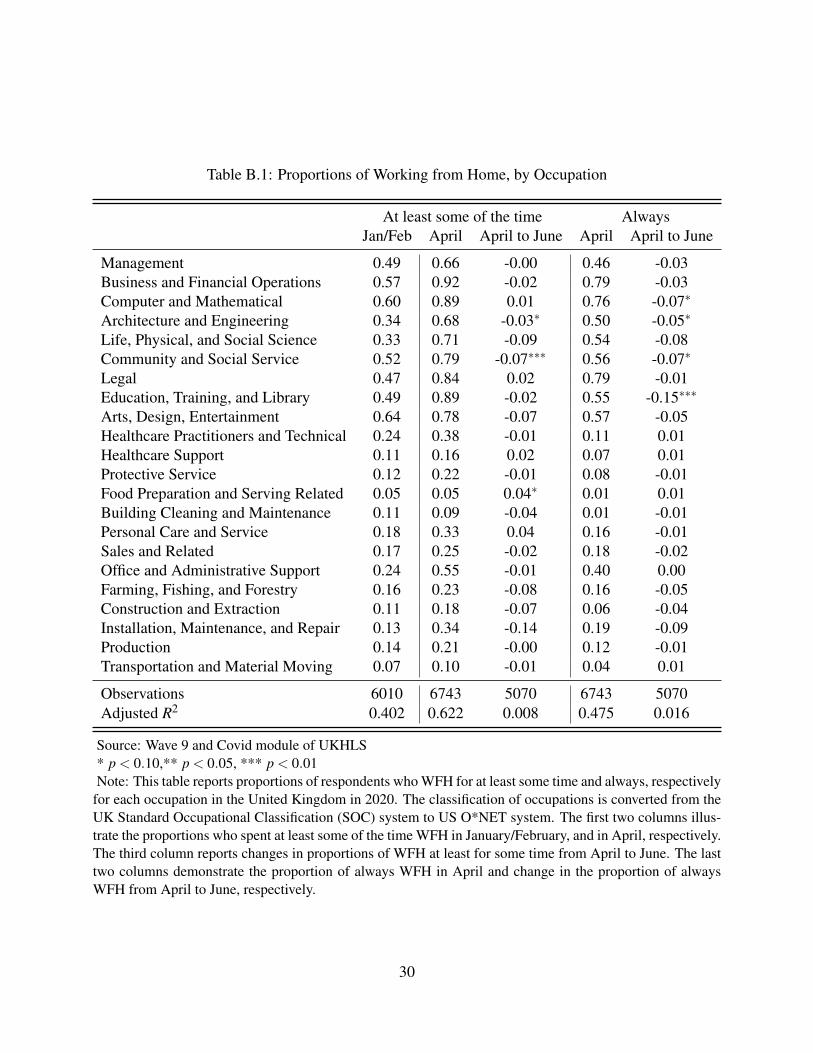
Table B.1: Proportions of Working from Home, by Occupation
At least some of the time AlwaysJan/Feb April April to June April April to June
Management 0.49 0.66 -0.00 0.46 -0.03Business and Financial Operations 0.57 0.92 -0.02 0.79 -0.03Computer and Mathematical 0.60 0.89 0.01 0.76 -0.07∗
Architecture and Engineering 0.34 0.68 -0.03∗ 0.50 -0.05∗
Life, Physical, and Social Science 0.33 0.71 -0.09 0.54 -0.08Community and Social Service 0.52 0.79 -0.07∗∗∗ 0.56 -0.07∗
Legal 0.47 0.84 0.02 0.79 -0.01Education, Training, and Library 0.49 0.89 -0.02 0.55 -0.15∗∗∗
Arts, Design, Entertainment 0.64 0.78 -0.07 0.57 -0.05Healthcare Practitioners and Technical 0.24 0.38 -0.01 0.11 0.01Healthcare Support 0.11 0.16 0.02 0.07 0.01Protective Service 0.12 0.22 -0.01 0.08 -0.01Food Preparation and Serving Related 0.05 0.05 0.04∗ 0.01 0.01Building Cleaning and Maintenance 0.11 0.09 -0.04 0.01 -0.01Personal Care and Service 0.18 0.33 0.04 0.16 -0.01Sales and Related 0.17 0.25 -0.02 0.18 -0.02Office and Administrative Support 0.24 0.55 -0.01 0.40 0.00Farming, Fishing, and Forestry 0.16 0.23 -0.08 0.16 -0.05Construction and Extraction 0.11 0.18 -0.07 0.06 -0.04Installation, Maintenance, and Repair 0.13 0.34 -0.14 0.19 -0.09Production 0.14 0.21 -0.00 0.12 -0.01Transportation and Material Moving 0.07 0.10 -0.01 0.04 0.01
Observations 6010 6743 5070 6743 5070Adjusted R2 0.402 0.622 0.008 0.475 0.016
Source: Wave 9 and Covid module of UKHLS* p < 0.10,** p < 0.05, *** p < 0.01Note: This table reports proportions of respondents who WFH for at least some time and always, respectively
for each occupation in the United Kingdom in 2020. The classification of occupations is converted from theUK Standard Occupational Classification (SOC) system to US O*NET system. The first two columns illus-trate the proportions who spent at least some of the time WFH in January/February, and in April, respectively.The third column reports changes in proportions of WFH at least for some time from April to June. The lasttwo columns demonstrate the proportion of always WFH in April and change in the proportion of alwaysWFH from April to June, respectively.
30
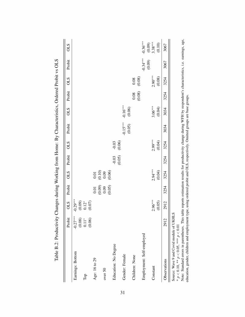
Tabl
eB
.2:P
rodu
ctiv
ityC
hang
esdu
ring
Wor
king
from
Hom
e:B
yC
hara
cter
istic
s,O
rder
edPr
obit
vsO
LS
Prob
itO
LS
Prob
itO
LS
Prob
itO
LS
Prob
itO
LS
Prob
itO
LS
Prob
itO
LS
Ear
ning
s:B
otto
m-0
.27∗∗∗
-0.2
9∗∗∗
(0.0
8)(0
.09)
Top
0.11∗
0.12∗
(0.0
6)(0
.07)
Age
:16
to29
0.01
0.01
(0.0
9)(0
.10)
over
500.
090.
09(0
.05)
(0.0
6)E
duca
tion:
No
Deg
ree
-0.0
3-0
.03
(0.0
5)(0
.06)
Gen
der:
Fem
ale
-0.1
5∗∗∗
-0.1
6∗∗∗
(0.0
5)(0
.06)
Chi
ldre
n:N
one
0.08
0.08
(0.0
8)(0
.08)
Em
ploy
men
t:Se
lf-e
mpl
oyed
-0.3
4∗∗∗
-0.3
6∗∗∗
(0.0
9)(0
.09)
Con
stan
t2.
96∗∗∗
2.94∗∗∗
2.99∗∗∗
3.06∗∗∗
2.90∗∗∗
3.38∗∗∗
(0.0
5)(0
.04)
(0.0
4)(0
.04)
(0.0
8)(0
.10)
Obs
erva
tions
2912
2912
3254
3254
3254
3254
3034
3034
3254
3254
3067
3067
Sour
ce:W
ave
9an
dC
ovid
mod
ule
ofU
KH
LS
*p<
0.10
,**
p<
0.05
,***
p<
0.01
Not
e:St
anda
rder
rors
inpa
rent
hese
s.T
his
tabl
ere
port
ses
timat
ion
resu
ltsfo
rpr
oduc
tivity
chan
gedu
ring
WFH
byre
spon
dent
’sch
arac
teri
stic
s,i.e
.ea
rnin
gs,a
ge,
educ
atio
n,ge
nder
,chi
ldre
nan
dem
ploy
men
ttyp
e,us
ing
orde
red
prob
itan
dO
LS,
resp
ectiv
ely.
Om
itted
grou
psar
eba
segr
oups
.
31